NBER WORKING PAPER SERIES

A COMPARISON OF MONETARY ANCHOR OPTIONS, INCLUDING PRODUCTPRICE TARGETING, FOR COMMODITY-EXPORTERS IN LATIN AMERICA

Jeffrey A. Frankel

Working Paper 16362http://www.nber.org/papers/w16362

NATIONAL BUREAU OF ECONOMIC RESEARCH1050 Massachusetts Avenue

Cambridge, MA 02138September 2010

This study was presented at a workshop on Myths and Realities of Commodity Dependence: PolicyChallenges and Opportunities for Latin America and the Caribbean, World Bank, Sept. 17-18, 2009.The author thanks Daniella Llanos for excellent research assistance. The views expressed herein arethose of the author and do not necessarily reflect the views of the National Bureau of Economic Research.

© 2010 by Jeffrey A. Frankel. All rights reserved. Short sections of text, not to exceed two paragraphs,may be quoted without explicit permission provided that full credit, including © notice, is given tothe source.

A Comparison of Monetary Anchor Options, Including Product Price Targeting, for Commodity-Exporters in Latin AmericaJeffrey A. FrankelNBER Working Paper No. 16362September 2010JEL No. E5,F4

ABSTRACT

Seven possible nominal variables are considered as candidates to be the anchor or target for monetarypolicy. The context is countries in Latin America and the Caribbean (LAC), which tend to be pricetakers on world markets, to produce commodity exports subject to volatile terms of trade, and to experienceprocyclical international finance. Three candidates are exchange rate pegs: to the dollar, euro andSDR. One candidate is orthodox Inflation Targeting. Three candidates represent proposals for anew sort of inflation targeting that differs from the usual focus on the CPI, in that prices of exportcommodities are given substantial weight and prices of imports are not: PEP (Peg the Export Price),PEPI (Peg an Export Price Index), and PPT (Product Price Targeting). The selling point of theseproduction-based price indices is that each could serve as a nominal anchor while yet accommodatingterms of trade shocks, in comparison to a CPI target. All seven nominal anchors deliver greater overallnominal price stability in our simulations than the inflationary historical monetary regimes actuallyfollowed by LAC countries (with the exception of Panama). A dollar peg does not particularly stabilizedomestic commodity prices. As hypothesized, a product price target generally does a better job ofstabilizing the real domestic prices of tradable goods than does a CPI target. CPI-targeters such asBrazil, Chile, and Peru respond to increases in world prices of imported oil with monetary policy thatis sufficiently tight to appreciate their currencies, an undesirable property. A Product Price targeteror PEP country would respond to increases in world prices of its commodity exports by appreciation,a desirable property.

Jeffrey A. FrankelKennedy School of GovernmentHarvard University79 JFK StreetCambridge, MA 02138and NBERjeffrey_frankel@harvard.edu

2

A Comparison of Monetary Anchor Options, Including Product Price Targeting, for Commodity-Exporters in Latin America

Introduction: The Evolution of Nominal Targets for Monetary Policy in Latin America and the Caribbean

In perhaps no other region have attitudes with respect to nominal anchors for

monetary policy evolved more than in the developing countries of the Western Hemisphere.

Inflation rates went very high in the early 1980s, to hyperinflation in some cases (including Argentina, Bolivia, Brazil, and Nicaragua). As a result, the need for a nominal anchor was plain to see. In a non-stochastic model, any nominal variable is as good a choice for monetary anchor as any other nominal variable. But in a stochastic model, not to mention the real world, it makes quite a difference what is the nominal variable toward which the monetary authorities publicly commit in advance. 1 Should it be the money supply? Exchange rate? CPI? Other alternatives?

When stabilization was finally achieved in the countries of Latin America and the Caribbean (LAC), in the 1980s and early 1990s, the exchange rate was virtually always the nominal anchor around which the successful stabilization programs were built, whether it was Chile’s tablita, Bolivia’s exchange rate target, Argentina’s convertibility plan, or Brazil’s real plan. But matters have continued to evolve. The trend from exchange rate targeting to inflation targeting

The series of emerging market currency crises that began in Mexico in December 1994 and ended in Argentina in January 2002 all involved the abandonment of exchange rate targets, in favor of more flexible currency regimes, if not outright floating. In many countries, the abandonment of a cherished exchange rate anchor for monetary policy took place under the urgent circumstances of a speculative attack (including Mexico and Argentina). A few countries made the jump to floating preemptively, before a currency crisis could hit (Chile and Colombia). Only a very few smaller countries responded to the ever rougher seas of international financial markets by moving the opposite direction, to full dollarization (Ecuador, under pressure of crisis; and El Salvador, out of longer-run motivations). On a 30-year time span, the general trend has been toward increased flexibility.2

1 The best reference for this familiar point is Rogoff (1985). Two appendices demonstrate the point in this study, that the choice of nominal target makes a big difference in the presence of shocks. 2 Collins (1996). The co-existence of floating, on the one hand, and currency boards and dollarization, on the other, gave rise in the late 1990s to the hypothesis that emerging market countries could go to either the floating corner or the institutionally fixed corner, but that intermediate exchange rate regimes such as

3

With exchange rate targets somewhat out of favor by the end of the 1990s, and the

gold standard and monetarism3 having been already relegated to the scrap heap of history, there was a clear vacancy for the position of Preferred Nominal Anchor, or intermediate target for monetary policy. The table in Appendix 1 summarizes, with historical examples, the Achilles heel or vulnerability of monetarism, the gold standard, and each of the other variables that have been proposed as candidates for nominal target. Appendix 2 illustrates the point with a theoretical model in the mode of Rogoff (1985).

The regime of Inflation Targeting (IT) was a fresh young face, coming with an already-impressive resume of recent successes in wealthier countries (New Zealand, Canada, United Kingdom, and Sweden). In many emerging market countries around the world, IT got the job of preferred nominal anchor. Three South American countries officially adopted Inflation Targeting in 1999, in place of exchange rate targets: Brazil, Chile, and Colombia.4 Mexico had done so earlier, after the peso crisis of 1994-95. Peru followed suit in 2002, switching from an official regime of money targeting. Guatemala has officially entered a period of transition to inflation targeting, under a law passed in 2002.

In many ways, Inflation Targeting has functioned well. It apparently anchored expectations and avoided a return to inflation in Brazil, for example, despite two severe challenges: the 50% depreciation of early 1999, as the country exited from the real plan, and the similarly large depreciation of 2002, when a presidential candidate who at the time was considered anti-market and inflationary pulled ahead in the polls.5

One could argue, however, that events of the past few years, particularly the global financial crisis of 2007-2009, have put strains on the Inflation Targeting regime much as the events of 1994-2001 had earlier put strains on the regime of exchange rate targeting. Three other kinds of nominal variables have forced their way into the attentions of central bankers, beyond the CPI. One nominal variable, the exchange rate, never really left – certainly not for the smaller countries. A second category of nominal variable, asset prices, has been the most relevant in the last few years in industrialized countries. The international financial upheaval that began in mid-2007 with the US sub-prime mortgage crisis has forced central bankers to re-think their intent focus on inflation, to the exclusion of equity and real estate prices. But a third category, prices of agricultural and mineral products, is particularly relevant for countries in Latin America

basket pegs or target zones were no longer viable. This “corners hypothesis” subsequently fell largely out of fashion, as one could have predicted. Frankel (2004). 3 Enthusiasm for monetarism had largely died out by the mid-1980s, perhaps because M1 targets had recently proven unrealistically restrictive in the largest industrialized countries. A surprising number of LAC countries continue officially to list money supply as their anchoring variable (Argentina, Guyana, Jamaica, and Uruguay). But one may doubt in practice how strictly they try to keep any monetary aggregate within declared ranges. 4 Chile had begun to set inflation targets in 1991, but had also followed a basket peg exchange rate target throughout the 1990s. Mishkin (2008) discusses the examples of Chile and Brazil. 5 Giavazzi, Goldfajn, and Herrera (2005). Skeptical investor perceptions of Luiz Inacio Lula da Silva were not entirely unreasonable at the time, based on the record of his past statements, but in the end were belied by his responsible policies when in office.

4

and the Caribbean. The greatly heightened volatility of commodity prices in the past decade, culminating in the price spike of 2008, has resurrected arguments about the desirability of a currency regime that accommodates terms of trade shocks. This third challenge to CPI-targeting is the one that receives the most attention in this study. What, exactly, is meant by Inflation Targeting?

Inflation targeting has sometimes been defined very broadly: “the monetary authorities choose a long run goal for inflation and act transparently.” 6 But usually something more specific is implied by the term. For one thing, the price target is virtually always the Consumer Price Index (though sometimes “core” rather than “headline” CPI). A contribution of this paper is to consider other price indices that are possible alternatives to the CPI for the role of nominal anchor, within what could still be called Inflation Targeting.

The narrow definition of inflation targeting would have the central bank governor committing each year to a goal for the CPI over the course of the coming year, and then putting 100% weight on achieving that objective to the exclusion of all others. Some proponents make clear that they are talking about something broader than this: flexible inflation targeting, under which the central bank puts some weight on the output objective rather than everything on the inflation objective – as in a Taylor Rule -- over the one-year horizon. This study will not deal especially with the eternal question of how much weight should be placed in the short term on a nominal anchor, such as a price index, relative to real output; nor with the question of how much discretion a central bank should be allowed, as opposed to strict adherence to a rule. The central focus will, rather, be on another specific question: to whatever extent weight is to be placed on a nominal anchor -- whether it is 100% as under a fixed exchange rate, or a more flexible range – what are the advantages and disadvantages of various nominal anchors? What is different about Latin American economies? Low credibility, procyclical finance, supply shocks, and terms of trade volatility Which regimes are most suitable for countries in the region? Table 1 reports the exchange rate and monetary regimes currently followed officially by 18 LAC countries. Inflation, the exchange rate, and the money supply are all represented among their choices of targets.7 We begin with a consideration of some structural characteristics that tend to differentiate these countries from others, though it is important to acknowledge tremendous heterogeneity within the region.8

6 Among many references in the large literature on inflation targeting, three that are internationally oriented are: Svensson (1995), Bernanke, Laubach, Mishkin, and Posen (1999); and Truman (2003).

7 Mishkin and Savastano (2002). 8 For a much more comprehensive consideration of the region’s structural characteristics, see: Loayza, Fajnzylber, and Calderón (2005).

5

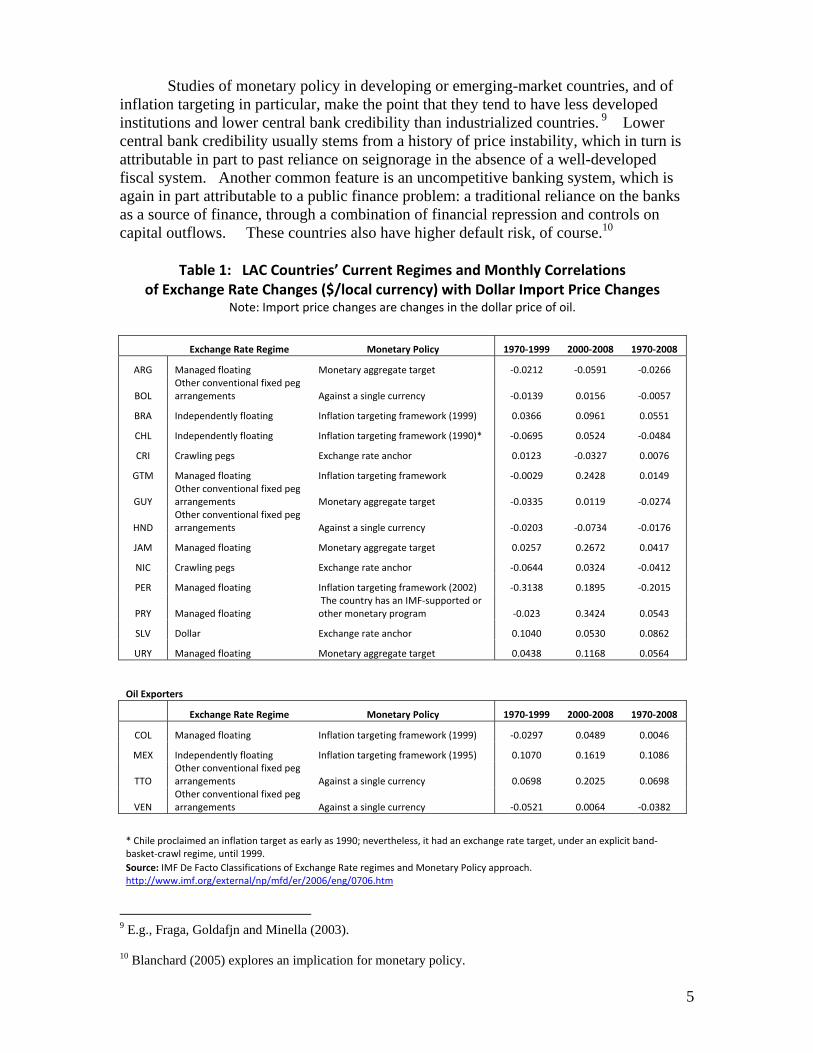
Studies of monetary policy in developing or emerging-market countries, and of inflation targeting in particular, make the point that they tend to have less developed institutions and lower central bank credibility than industrialized countries. 9 Lower central bank credibility usually stems from a history of price instability, which in turn is attributable in part to past reliance on seignorage in the absence of a well-developed fiscal system. Another common feature is an uncompetitive banking system, which is again in part attributable to a public finance problem: a traditional reliance on the banks as a source of finance, through a combination of financial repression and controls on capital outflows. These countries also have higher default risk, of course.10

Table 1:   LAC Countries’ Current Regimes and Monthly Correlations  

of Exchange Rate Changes ($/local currency) with Dollar Import Price Changes        Note: Import price changes are changes in the dollar price of oil. 

                 

   Exchange Rate Regime  Monetary Policy  1970‐1999  2000‐2008  1970‐2008 

ARG  Managed floating  Monetary aggregate target  ‐0.0212  ‐0.0591  ‐0.0266 

BOL Other conventional fixed peg arrangements  Against a single currency  ‐0.0139  0.0156  ‐0.0057 

BRA  Independently floating  Inflation targeting framework (1999)  0.0366  0.0961  0.0551 

CHL  Independently floating  Inflation targeting framework (1990)*  ‐0.0695  0.0524  ‐0.0484 

CRI  Crawling pegs  Exchange rate anchor  0.0123  ‐0.0327  0.0076 

GTM  Managed floating  Inflation targeting framework  ‐0.0029  0.2428  0.0149 

GUY Other conventional fixed peg arrangements  Monetary aggregate target  ‐0.0335  0.0119  ‐0.0274 

HND Other conventional fixed peg arrangements  Against a single currency  ‐0.0203  ‐0.0734  ‐0.0176 

JAM  Managed floating  Monetary aggregate target  0.0257  0.2672  0.0417 

NIC  Crawling pegs  Exchange rate anchor  ‐0.0644  0.0324  ‐0.0412 

PER  Managed floating  Inflation targeting framework (2002)  ‐0.3138  0.1895  ‐0.2015 

PRY  Managed floating  The country has an IMF‐supported or other monetary program  ‐0.023  0.3424  0.0543 

SLV  Dollar  Exchange rate anchor  0.1040  0.0530  0.0862 

URY  Managed floating  Monetary aggregate target  0.0438  0.1168  0.0564 

                 

Oil Exporters             

   Exchange Rate Regime  Monetary Policy  1970‐1999  2000‐2008  1970‐2008 

COL  Managed floating  Inflation targeting framework (1999)  ‐0.0297  0.0489  0.0046 

MEX  Independently floating  Inflation targeting framework (1995)  0.1070  0.1619  0.1086 

TTO Other conventional fixed peg arrangements  Against a single currency  0.0698  0.2025  0.0698 

VEN Other conventional fixed peg arrangements  Against a single currency  ‐0.0521  0.0064  ‐0.0382 

                 * Chile proclaimed an inflation target as early as 1990; nevertheless, it had an exchange rate target, under an explicit band‐basket‐crawl regime, until 1999.  

Source: IMF De Facto Classifications of Exchange Rate regimes and Monetary Policy approach.      http://www.imf.org/external/np/mfd/er/2006/eng/0706.htm   

9 E.g., Fraga, Goldafjn and Minella (2003). 10 Blanchard (2005) explores an implication for monetary policy.

6

 

The standardly drawn implications of underdeveloped institutions and low inflation-fighting credibility are that it is particularly important (i) that their central banks have independence11 and (ii) that they make regular public commitments to a transparent and monitorable nominal target. Some Latin American countries have given their central banks legal independence, beginning with Chile, Colombia, Mexico, and Venezuela in the 1990s.12 Sure enough, Jácome (2001), Gutiérez (2003) and Jácome and Vázquez (2008) find a negative statistical relationship between central bank independence and inflation among LAC countries. There are also some skeptics, however, who argue that central bank independence won’t be helpful if a country’s political economy dictates budget deficits regardless of monetary policy. 13 The principle of commitment to a nominal anchor in itself says nothing about what economic variables are best suited to play that role. Public promises to hit targets that cannot usually be fulfilled subsequently will do little to establish credibility.14

Most analysis of inflation targeting is more suited to large industrialized countries than to small developing countries, in several respects.15 First, the theoretical models usually do not feature a role for exogenous shocks in trade conditions or difficulties in the external accounts. The theories tend to assume that countries need not worry about financing trade deficits internationally. Many assume that international capital markets function well enough to smooth consumption in the face of external shocks.16 In reality, however, financial market imperfections are serious for developing countries.17 International capital flows often exacerbate external shocks, rather than moderating them. Booms -- featuring capital inflows, excessive currency overvaluation and associated current account deficits -- are often followed by busts, featuring sudden stops in inflows,

11 E.g., Cukierman, Miller and Neyapti (2002). 12 Junguito and Vargas (1996) and Anone, Laurens and Segalotto (2006). 13 Mas (1995). 14 The Bundesbank had enough credibility that a record of proclaiming M1 targets and then missing them did little to undermine its reputation or expectations of low inflation in Germany. Latin America does not enjoy the same luxury. 15 This is not to forget the many studies of inflation targeting for emerging market and developing countries. They include Debelle (2001); Fraga, Goldfajn, and Minella (2003); McKibbin and Singh (2003); Mishkin (2000; 2004); and Laxton and Pesenti (2003). Savastano (2000) offers offered a concise summary of much of the research as of that date. 16 One of the few exceptions is Caballero and Krishnamurthy (2003).

17 See Caballero (2000) and comments thereon.

7

abrupt depreciation, and recession.18 An analysis of monetary policy that did not take into account the international financial crises of 1982, 1994-2001, or 2008-09 would not be useful to policy makers in Latin America and the Caribbean.

Capital flows are particularly prone to exacerbate fluctuations when the source of the fluctuations is trade shocks.19 This observation leads us to the next relevant respect in which developing countries differ from industrialized countries.

Analysis of how IT works in practice sometimes gives insufficient attention to the consequences of supply shocks. Supply shocks tend to be larger for developing countries than for industrialized countries. One reason is the larger role of farming, fishing, and forestry in the economy. Droughts, floods, hurricanes, and other weather events – good as well as bad -- tend to have a much larger effect on GDP in developing countries. When a hurricane hits a Caribbean island, it can virtually wipe out the year’s banana crop and tourist season – thus eliminating the two biggest sectors in some of those tropical economies. A second reason for larger supply shocks is terms of trade volatility, which is notoriously high for small developing countries. This is especially true of those dependent on agricultural and mineral exports.20 Another feature of these countries is that they tend to be more dependent on imported inputs. In large rich countries, the fluctuations in the terms of trade are both smaller and less likely to be exogenous. (For industrialized countries that float, terms of trade fluctuations are dominated by variation in the nominal exchange rate.21 For industrialized countries that firmly fix, fluctuations are much smaller.)

As has been shown by a variety of authors, Inflation Targeting (defined narrowly) is not robust with respect to supply shocks.22 Under strict IT, to prevent the price index from rising in the face of an adverse supply shock monetary policy must tighten so much that the entire brunt of the fall in nominal GDP is borne by real GDP. Most reasonable objective functions would, instead, tell the monetary authorities to allow part of the temporary fall in nominal income to show up as an increase in the price level. Of course this is precisely the reason why many IT proponents favor flexible inflation targeting, often in the form of the Taylor Rule which does indeed call for the central bank to share the pain between inflation and output. It is also a reason for pointing to the “core” CPI rather than “headline” CPI. But these accommodations are insufficient. 18 Calvo, Leiderman and Reinhart (1993); Kaminsky, Reinhart, and Vegh (2005); Reinhart and Reinhart (2009); Perry (2009); Gavin, Hausmann, Perotti, and Talvi (1997); Gavin, Hausmann and Leiderman (1996); Mendoza and Terrones (2008).

19 E.g., Hausmann and Rigobon (2003). 20 E.g., Fraga, Goldfajn, and Minella, op cit. The old structuralist school in Latin America believed that specialization in primary commodities was undesirable because they faced a low elasticity of demand. 21 E.g., Taylor (2002). 22Among other examples: Frankel (1985) ; Frankel, Smit, and Sturzenegger (2008).

8

“Headline” CPI, Core CPI, and Nominal Income Targeting

In practice, inflation-targeting central bankers usually say they respond to large temporary shocks in the prices of oil and other agricultural and mineral products by excluding them from the measure of the CPI that is targeted. Central banks have two approaches to doing this. Some publicly explain ex ante that their target for the year is inflation in the Core CPI, a measure that excludes volatile components, usually farm and energy products. The virtue of this approach is that the central banks are able to abide by their public commitments when the supply shock comes. (This logic assumes the shock is located in the agricultural or energy sectors. It doesn’t work, for example, for labor unrest or power failures that disrupt industrial activity.) The disadvantage of declaring core CPI as the official target is that the person in the street is less likely to understand it, compared to the simple CPI. Transparency and communication of a target that the public can monitor are the original reasons for declaring a specific nominal target in the first place.

The alternative approach is to talk about the ordinary CPI ex ante, but then in the face of an adverse supply shock explain ex post that the increase in farm or energy prices is being excluded due to special circumstances. This strategy can be a public relations disaster. The people in the street are told that they shouldn’t be concerned by the increase in the CPI because it is “only” occurring in the cost of filling up their auto fuel tanks and buying their weekly groceries. Either way, ex ante or ex post, the effort to explain away supply-induced fluctuations in the CPI undermines the credibility of the monetary authorities. This credibility problem is especially severe in countries where there are serious grounds for believing that government officials fiddle with the consumer price indices for political purposes, which includes Argentina (recently) and Brazil (in the more distant past), among others.

Given the value that most central bankers place on transparency and their reputations, it would be surprising if their public emphasis on the CPI did not lead them to be at least a bit more contractionary in response to adverse supply shocks, and expansionary in response to favorable supply shocks, than they would be otherwise. In other words, it would be surprising if they felt able to take full advantage of the escape clause offered by the idea of core CPI. There is some reason to think that this is indeed the case. A simple statistic: the exchange rates of all major inflation-targeting countries (in dollars per national currency) are positively correlated with the dollar price on world markets of their import baskets.23 Why is this fact revealing? The currency should not respond to an increase in world prices of its imports by appreciating, to the extent that these central banks target core CPI (and to the extent that the commodities excluded by core CPI include all imported commodities that experience world price shocks, which is a big qualifier). If anything, floating currencies should depreciate in response to such an adverse terms of trade shock. When these IT currencies respond by appreciating instead, it suggests that the central bank is tightening monetary policy to reduce upward pressure on the CPI.

Three columns of Table 1 repeat the correlation calculations for our LAC countries, on monthly data. We take the example of dollar oil prices, since they are the most important source of variation in dollar import prices, for oil-importing countries. 23 Frankel (2005).

9

Six of the 18 countries are inflation targeters currently. We might exclude Guatemala, because its transition to inflation targeting is recent, and perhaps not even complete. We should also exclude those LAC countries that are oil producers. Regardless, every one of the inflation targeters shows correlations between dollar import pries and the dollar values of their currencies that are both positive over the period 2000-2008 and greater than the correlations during the pre-IT period. The evidence supports the idea that in the LAC region as well, inflation targeters – in particular, Brazil, Chile and Peru -- tended to react to the positive oil shocks of the past decade by tightening monetary policy and thereby appreciating their currencies. The implication seems to be that the CPI which they target does not in practice entirely exclude oil price shocks. Apparently “flexible inflation targeting” is not quite as flexible as one would think. (Argentina, by contrast, is not an inflation targeter, and allows its peso to depreciate when world prices of its import goods rise.)

What is wanted as candidate for nominal target is a variable that is simpler for the public to understand ex ante than core CPI, and yet that is robust with respect to supply shocks. Being robust with respect to supply shocks means that the central bank should not have to choose ex post between two unpalatable alternatives: an unnecessary economy-damaging recession or an embarrassing credibility-damaging violation of the declared target.

One variable that fits the desirable characteristics is nominal GDP.24 Nominal income targeting is a regime that has the desirable property of taking supply shocks partly as P and partly as Y, without forcing the central bank to abandon the declared nominal anchor. The proposal was popular among macroeconomists in the 1980s.25 Some critics claimed that nominal income targeting was less applicable to developing countries because of long lags and large statistical errors in measurement. But these measurement problems are smaller in most developing countries than they used to be. Furthermore, the fact that developing countries are more vulnerable to supply shocks than are industrialized countries suggests that the proposal is more applicable to them, not less, as McKibbin and Singh (2003) have pointed out.

In any case, for some reason, nominal income targeting has not been seriously considered since the 1990s, either by rich or poor countries. Thus it will not be analyzed in this paper. Fortunately, nominal income is not the only variable that is more robust to supply shocks than the CPI.

24 Nominal demand would probably be better than nominal income, for some technical reasons (excluding the trade balance and, if possible, unintended inventory accumulation). But it does not pass the test of being easily perceived and understood by the public. 25 It was plain to see the superiority of nominal GDP targeting when the status quo was M1 targeting . (Indeed, the proposal for nominal income targeting might have been better received by central banks if it had been called “Velocity-Shift-Adjusted Money Targeting.”) Bean (1983); Feldstein and Stock (1994); Frankel (1995); Taylor (1985); Tobin (1980); West (1986).

10

Terms of trade shocks

If the supply shocks are terms of trade shocks, then the choice of CPI to be the price index on which IT focuses is particularly inappropriate. The alternative is an output-based price index such as an index of export prices, the GDP deflator, the Producer Price Index, or a specially constructed Product Price Index. The important difference is that imported goods show up in the CPI, but not in the output-based price indices and vice versa for exported goods: they show up in the output-based prices but much less in the CPI. Proponents of inflation targeting do not seem to have considered this point. One reason may be that the difference is not, in fact, as important for large industrialized countries as for small developing countries, especially those that export mineral and agricultural products.

Terms of trade volatility is particularly severe for commodity exporters, which includes most countries in Latin America and the Caribbean. Some LAC countries have a large share of their exports concentrated in a product – such as coffee, copper, or oil -- that is so volatile that it periodically experiences swings in world market conditions that double or halve their prices. The export markets for the manufactured goods and services produced by industrialized countries, on the other hand, tend to be much more stable. This is especially true for the larger industrialized countries such as the United States, who have more monopoly power and whose exports are more diversified.

11

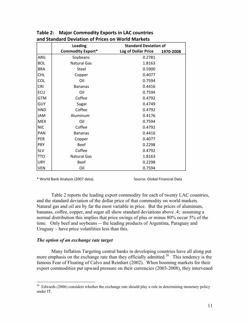
Table 2:    Major Commodity Exports in LAC countries  and Standard Deviation of Prices on World Markets 

* World Bank Analysis (2007 data).                                           Source: Global Financial Data  

Table 2 reports the leading export commodity for each of twenty LAC countries,

and the standard deviation of the dollar price of that commodity on world markets. Natural gas and oil are by far the most variable in price. But the prices of aluminum, bananas, coffee, copper, and sugar all show standard deviations above .4; assuming a normal distribution this implies that price swings of plus or minus 80% occur 5% of the time. Only beef and soybeans -- the leading products of Argentina, Paraguay and Uruguay – have price volatilities less than this. The option of an exchange rate target

Many Inflation Targeting central banks in developing countries have all along put more emphasis on the exchange rate than they officially admitted.26 This tendency is the famous Fear of Floating of Calvo and Reinhart (2002). When booming markets for their export commodities put upward pressure on their currencies (2003-2008), they intervened

26 Edwards (2006) considers whether the exchange rate should play a role in determining monetary policy under IT.

Leading  Commodity Export*

     Standard Deviation of  Log of Dollar Price 1970‐2008

ARG Soybeans 0.2781

BOL Natural Gas 1.8163

BRA Steel 0.5900

CHL Copper 0.4077

COL Oil 0.7594

CRI Bananas 0.4416

ECU Oil 0.7594

GTM Coffee 0.4792

GUY Sugar 0.4749

HND Coffee 0.4792

JAM Aluminum 0.4176

MEX Oil 0.7594

NIC Coffee 0.4792

PAN Bananas 0.4416

PER Copper 0.4077

PRY Beef 0.2298

SLV Coffee 0.4792

TTO Natural Gas 1.8163

URY Beef 0.2298

VEN Oil 0.7594

12

heavily to dampen appreciation. Colombia was one of many examples.27 Then, when the world financial crisis hit in 2007, and especially when it put more severe downward pressure on their currencies in the latter part of 2008 -- partly in the form of an abrupt reversal of the commodity price spike -- some of these same countries intervened heavily to dampen the depreciation of their currencies. The point is that central banks still do – and should – pay a lot of attention to their exchange rates.

The point applies to the entire spectrum from managed floaters to peggers. Fixed exchange rates are still an option to be considered for many countries, especially small ones. For very small countries, especially those that are highly integrated with the United States (many countries in Central America and the Caribbean, in particular), an institutional peg or even full dollarization remain reasonable options. Fixed exchange rates have many advantages, in addition to their use as a nominal anchor for monetary policy. They reduce transactions costs and exchange risk, which in turn facilitates international trade and investment. This is especially true for institutionally locked-in arrangements, such as dollarization. Influential research by Rose (2000) and others over the last decade has shown that fixed exchange rates and, especially, monetary unions, increase trade and investment substantially. In addition they avoid the speculative bubbles to which floating exchange rates are occasionally subject.

Of course fixed exchange rates have disadvantages too. Most importantly, to the extent financial markets are integrated, a fixed exchange rate means giving up monetary independence; the central bank can’t increase the money supply, lower the interest rate, or devalue the currency, in response to a downturn in demand for its output.

It has been argued that Latin American governments have misused monetary discretion more often than they have used it to achieve the textbook objectives, so that the loss of monetary independence under a fixed exchange rate is not to be lamented. A second disadvantage of a fixed rate, however, presupposes no discretionary abilities: it means giving up the automatic accommodation of trade shocks that comes with floating: a depreciation when world market conditions for the export commodity weaken, and vice versa.28 Berg, Borensztein, and Mauro (2003) say it well:

“Another characteristic of a well-functioning floating exchange rate is that it responds appropriately to external shocks. When the terms of trade decline, for example, it makes sense for the country’s nominal exchange rate to weaken, thereby facilitating the required relative price adjustment. Emerging market floating exchange rate countries do, in fact, react in this way to negative terms of trade shocks. In a large sample of developing countries over the past three decades, countries that have fixed exchange rate regimes and that face negative terms of trade shocks achieve real exchange rate depreciations only with a lag of two years while suffering large real GDP declines. By contrast, countries with floating rates display large nominal and real depreciations on impact and later suffer some inflation but much smaller output losses.” Besides the inability to respond monetarily to shocks, there are three more

disadvantages of rigidity in exchange rate arrangements. It can impair the central bank’s lender of last resort capabilities in the event of a crisis in the banking sector, as Argentina demonstrated in 2001. It entails a loss of seignorage, especially for a country that goes

27 Vargas (2005) 28 Among peggers, terms-of-trade shocks are amplified and long-run growth is reduced, as compared to flexible-rate countries, according to Edwards and Yeyati (2005). Also see Broda (2004).

13

all the way to dollarization. And, finally, for a country that stops short of full dollarization, pegged exchange rates are occasionally subject to unprovoked speculative attacks (of the “second-generation” type29). Econometric attempts to discern what sort of regime delivers the best economic performance across countries – firmly fixed, floating, or intermediate – have not been successful.30 Clearly the answer depends on the circumstances of the country in question. A list of criteria that qualify a country for a relatively firm fixed exchange rate, versus a more flexible rate, should include at least these eight characteristics:

1. Small size. 2. Openness, as reflected, for example, in the ratio of tradable goods to GDP.31 In

the simple model of Appendix 2, a sufficient (but not necessary) condition for PEP to dominate an exchange rate target is if the traded commodity sector is larger than the nontraded goods sector.

3. Less exposure to external shocks than to domestic and monetary shocks. Again, high variability in the terms of trade makes it more likely that a floating exchange rate dominates a pegged exchange rate. A conclusion of the model of Appendix 2 is that high variability in export markets also makes it more likely that PEP dominates a pegged exchange rate.32

4. The existence of a major-currency partner with whom bilateral trade, investment and other activities are already high, or are hoped to be high in the future.

5. “Symmetry of shocks,” meaning high correlation of cyclical fluctuations between the home country and the country that determines policy regarding the money to which pegging is contemplated. This is important because, if the domestic country is to give up the ability to follow its own monetary policy, it is better if the interest rates chosen by the larger partner are more often close to those that the domestic country would have chosen anyway.33

6. Labor mobility. When monetary response to an asymmetric shock has been precluded, it is useful if workers can move from the high-unemployment region to the low-unemployment region.34 This is the primary mechanism of adjustment across states within the monetary union which is the United States.

7. Countercyclical remittances. In any given year, inflows or outflows of migration are a relatively small fraction of the labor force. Emigrant’s remittances, however, (i) constitute a large share of foreign exchange earnings in many developing countries, (ii) are variable, (iii) appear to be countercyclical.35 This is particularly important for Mexico, Central America and the Caribbean,

29 Obstfeld (1986). 30 Levy-Yeyati and Sturzenegger (2003) find that floats do a better job than firmly fixed rates or intermediate regimes. Unfortunately, other equally reputable studies find that floats do the best or that intermediate regimes do the best. 31 The classic reference is McKinnon (1963). 32 Because small countries tend to be less diversified in their exports, criterion 3 can be somewhat at odds with criterion 1. 33 Mundell (1961); Bayoumi and Eichengreen(1994). Applications to Latin America include: Foresti (2007), and Yeyati and Sturzennegger (2000). 34 Mundell, op cit. 35 Frankel (2010), and other references cited therein.

14

which send many emigrants to the United States, and receive a lot of remittances back. Of course, when there is a recession in the United States, as 2007-09, a loss in remittances is another way that the downturn is painfully transmitted to the migrant’s country of origin. But the point here is not to tally the effects of migration and remittances per se. The point is, rather, that remittances seem to respond to the difference between the cyclical positions of the sending and receiving country, which makes it a bit easier for the developing country to give up the option of setting a lower interest rate than the United States sets.36

8. Countercyclical fiscal transfers. Within the United States, if one region suffers an economic downturn, the federal fiscal system cushions it; one estimate is that for every dollar fall in the income of a stricken state, disposable income falls by only 70 cents. Perhaps the IMF, World Bank, and Interamerican Development Bank play this role to some degree in the Western Hemisphere. But such fiscal cushions are mostly absent at the international level. (Even where substantial transfers exist, they are rarely very countercyclical.)

9. Political willingness to give up some monetary sovereignty. Some countries look on their currency with the same sense of patriotism with which they look on their flag. It is not a good idea to force subordination to the US dollar (or the euro or any other foreign currency) down the throats of an unwilling public. Otherwise, in times of economic difficulty, the public is likely to blame Washington, D.C. (or Frankfurt).

For Mexico, Central America, most of the Caribbean, and the northwestern part of

South America, an exchange rate target would naturally mean a dollar target, because so much of their trade and other transactions are with the United States. But Argentina, Brazil and Chile trade roughly as much with Europe (or, for that matter, East Asia) as they do with the United States. To peg to the dollar is to introduce volatility vis-à-vis Europe, Japan, and other important trading partners. For them, one must not take as given that the relevant anchor currency would be the dollar. It could be the euro or, more likely, a weighted basket. One possibility is the SDR.37

In 2001, when Argentina’s rigid peg to the dollar was in its death throes, it was observed that the country’s trade problems could in a sense be attributed to the original 1991 decision to link to the currency of a country with which Argentina traded relatively little, and to the subsequent 1995-2001 appreciation of the dollar against the euro, Brazilian real, and currencies of other major trading partners, as much as it could be attributed to the rigidity of the regime per se. The alternative of a basket that would be half dollars and half euros was apparently considered by the authorities at that time. Among the eight monetary regimes to be considered in this study are three exchange rate targets: a peg to the dollar, a peg to the euro, and a peg to the SDR.

36 For example, Lake (2006) finds that, even though remittances into Jamaica fall when US income falls, they do respond to the difference between US and Jamaican income. 37 The SDR was newly revived as a component of the international monetary system in April 2009, by a summit of the G-20 in London.

15

Other choices for price index for inflation targeting As noted, of the possible price indices that a central bank could target, the CPI is the usual choice. The CPI is indeed the natural candidate to be the measure of the inflation objective for the long-term. But it may not be the best choice for intermediate target on an annual basis. There is a case to be made for targeting, in place of the CPI, either the producer price index (PPI) or an export price index (PEPI). The latter idea is a moderate version of a more exotic proposed monetary regime that I have written about elsewhere, called Peg the Export Price – or PEP, for short.38 PEP I have proposed PEP explicitly for those countries that happen to be heavily specialized in the production of oil or some other particular mineral or agricultural export commodity. (The original idea was a very special case: an African gold exporter could consider going on the gold standard.39) The proposal is to fix the price of that commodity in terms of domestic currency. For example, Chile would peg its currency to copper – in effect adopting a metallic standard. Ecuador, Trinidad and Venezuela would peg to oil.40 Jamaica would peg to bauxite. The Dominican Republic would peg to sugar. Central American coffee producers would peg to coffee. Argentina would peg to soybeans. And so forth.

How would this work operationally? Conceptually, one can imagine the government holding reserves of gold or copper or oil, and buying and selling the commodity whenever necessary to keep the price fixed in terms of local currency. Operationally, a more practical method would be for the central bank each day to announce an exchange rate vis-à-vis the dollar, following the rule that the day’s exchange rate target (dollars per local currency unit) moves precisely in proportion to the day’s price of gold or copper or oil on the New York market (dollars per commodity). Then the central bank could intervene via the foreign exchange market to achieve the day’s target. The dollar would be the vehicle currency for intervention -- precisely as it has long been when a small country defends a peg to some non-dollar currency. Either way, the effect would be to stabilize the price of the commodity in terms of local currency. Or perhaps, since these commodity prices are determined on world markets, a better way to express the same policy is stabilizing the price of local currency in terms of the commodity.

The argument for the export targeting proposal, relative to an exchange rate

target, can be stated succinctly: It delivers one of the main advantages that a simple exchange rate peg promises, namely a nominal anchor, while simultaneously delivering one of the main advantages that a floating regime promises, namely automatic adjustment in the face of fluctuations in world prices of the countries’ exports. Textbook theory says that when there is an adverse movement in the terms of trade, it is desirable to

38 Frankel and Saiki (2002) and Frankel (2003). 39 Frankel (2002). 40 In recent years – especially as a result of the large increase in world oil prices toward the end of our statistical sample – oil became the leading export commodity of Brazil and Colombia, both of whom traditionally export coffee and a wide variety of other goods.

16

accommodate it via a depreciation of the currency. When the dollar price of exports rises, under PEP the currency per force appreciates in terms of dollars. When the dollar price of exports falls, the currency depreciates in terms of dollars. Such accommodation of terms of trade shocks is precisely what is wanted. In past currency crises, countries that have suffered a sharp deterioration in their export markets have often eventually been forced to give up their exchange rate targets and devalue anyway. The adjustment was far more painful -- in terms of lost reserves, lost credibility, and lost output -- than if the depreciation had happened automatically. The desirability of accommodating terms of trade shocks is also a particularly good way to summarize the attractiveness of export price targeting relative to the reigning champion, CPI targeting. Consider the two categories of adverse terms of trade shocks: first, a fall in the dollar price of the export in world markets and, second, a rise in the dollar price of the import on world markets. In the first case, a fall in the export price, one wants the local currency to depreciate against the dollar. As already noted, PEP delivers that result automatically; CPI targeting does not. In the second case, a rise in the import price, the terms-of-trade criterion suggests that one again might want the local currency to depreciate. Neither regime delivers that result.41 But CPI targeting actually has the implication that the central bank tightens monetary policy so as to appreciate the currency against the dollar, by enough to prevent the local-currency price of imports from rising. This implication – reacting to an adverse terms of trade shock by appreciating the currency – is perverse. It can be expected to exacerbate swings in the trade balance and output. PEPI

Some have responded to the PEP proposal by pointing out, quite correctly, that the side-effect of stabilizing the local-currency price of the export commodity in question is that it would destabilize the local-currency price of other export goods. If agricultural or mineral commodities constitute virtually all of exports, then this may not be an issue. But for a heavy majority of countries, including most of those in Latin America and the Caribbean, no single commodity constitutes more than half of exports. Moreover, even those that are heavily specialized in a single mineral or agricultural product may wish to encourage diversification further into new products in the future, so as to be less dependent on that single commodity. For these two sorts of countries, the strict version of PEP is not appropriate. For those countries where export diversification is important, a moderated version of PEP is more likely to be suitable. One way to moderate the proposal is to interpret it as targeting a broad index of all export prices, rather than the price of only one export commodity. I have abbreviated this moderate form of the proposal as PEPI, for Peg the Export Price Index.42

Some countries are intermediate with respect to the extent of diversification: Exports are dominated by agricultural and mineral commodities, but it is a diversified

41 There is a reason for that. In addition to the goal of accommodating terms of trade shocks, there is also the goal of price instability; but to depreciate in the face of an increase in import prices would exacerbate inflation. 42 Frankel (2005).

17

basket of commodities, rather than just oil or coffee. Examples include Argentina (soybeans, wheat, maize and beef), Bolivia (hydrocarbons, zinc, soybeans, iron ore and tin) or Jamaica (bauxite, sugar, bananas, rum and coffee). In that case, the natural price index would be a basket of those four or five commodity prices, omitting manufactures and services for simplicity.

The proposal is not to be confused, however, with proposals in the 1930s or 1980s

to improve on the gold standard by targeting a diversified basket of commodities.43 Those proposals explicitly included the prices of imported commodities in the index. e.g., oil for an oil-importer The PEPI proposal explicitly excludes them. It also includes commodities that may be minor and obscure from the world’s viewpoint but important from the viewpoint of the producing country.44 These two differences are crucial when the terms of trade fluctuate. PPT

A way to moderate the proposal still further is to target a broad index of all domestically produced goods, whether exportable or not. PPT stands for Product Price Targeting. The GDP deflator is one possible output-based price index, but has the disadvantage of only being available quarterly, and being subject to lags in collection, measurement errors, and subsequent revisions. The PPI is superior in that – just like the CPI – it is generally collected monthly. Even in a small poor country with limited capacity to gather statistics, government workers can survey a sample of firms every month to construct a primitive PPI as easily as they can survey a sample of retail outlets to construct a primitive CPI. The PPI is a familiar non-threatening variable; inflation targeters should be open-minded enough to consider it as an alternative to the CPI. A possible disadvantage of the PPI as traditionally calculated (the old Wholesale Price Index) is that it weights products according to their shares in gross sales by businesses. An implication is that raw materials and other inputs get counted multiple times, because they are reflected in each gross sales price. It would probably be better to weight product prices by their share of the product’s value added in GDP, rather than the share of their gross value.45 A simple product price index could be computed monthly by surveying major establishments, and applying to their price changes the sectoral weights that are taken from longer-term GDP data.

Targeting the price index If a broad index of export or product prices were to be the nominal target, it

would of course be impossible in practice for the central bank to hit the target exactly, in contrast to the way that it is possible to hit virtually exactly a target for the exchange rate, the price of gold, or even the price of a basket of four or five exchange-traded agricultural or mineral commodities. There would instead be a declared band for the price index target, which could be wide if desired, just as with the targeting of the CPI, money 43 In the 1930s: Graham (1937); and Keynes (1938). In the 1980s: Hall (1982, 1985). 44 Such as antimony, tungsten and lithium, for the case of Bolivia. 45 The US Bureau of Economic Analysis took a step in this direction in 2007, when it began releasing a new index of aggregate net output prices. This index at least nets out double-counting of transactions within each aggregate industry.

18

supply, or other nominal variables. Open market operations to keep the export price index inside the band if it threatens to stray outside could be conducted in terms either of foreign exchange or in terms of domestic securities.

For some countries, it might help to monitor on a daily or weekly basis the price of a basket of agricultural and mineral commodities that is as highly correlated as possible with the country’s overall price index, but whose components are observable on a daily or weekly basis in well-organized markets. The central bank could even announce what the value of the basket index would be one week at a time, by analogy with the Fed funds target in the United States. The weekly targets could be set so as to achieve the medium-term goal of keeping the comprehensive price index inside the pre-announced bands; and yet the central bank could hit the weekly targets very closely, if it wanted, for example, by intervening in the foreign exchange market. This feature would enhance transparency from the viewpoint of those who operate in financial markets, even though the average household should not realistically be expected to follow such arcane details.

Analysis of competing monetary targets with respect to ability to stabilize relative prices

The remainder of this paper is a counterfactual analysis of alternative monetary

regimes. We examine a set of countries in Latin America and the Caribbean, and we compare the historical paths of prices under the historical monetary regime with what would have happened under eight other possible regimes: dollar target, euro target, SDR target, CPI target, PEP target, PEPI target, and PPI target. For simplicity, we assume that the targets are hit precisely, even though we realize that in a stochastic model this would not be possible with half the regimes (the price index targets). Sectoral weights in the price indices

The countries we are interested in are small open economies. Thus we assume that the law of one price holds, for commodity exports as well as for other exportables and importables, and that the prices of these goods are exogenous in world markets, that is, in terms of dollars. Thus the local-currency prices of the tradable goods are given by the exchange rate (actual or hypothetical, as the case may be) times the dollar prices.

The price index for non-traded goods is determined differently, however. They are not subject to the law of one price. Indeed, if all goods were subject to the law of one price, then the choice of currency regime would not make very much difference. The choice of monetary regime does make a difference, primarily because wages and prices of nontraded goods are sticky in the short run in terms of whatever is the local currency. In the longer run, however, purchasing power parity holds. Thus, in the case of the dollar peg, the local inflation rate – including nontraded goods – converges to the global inflation rate, which is here for simplicity taken to be that of the United States. Inasmuch as many Latin American countries suffered very high inflation rates in the

19

1970s and 1980s, even hyperinflations, it makes a big difference whether the counterfactual to the historical experience is that the country was credibly and rigorously tied to a nominal target all along, or that the country would have switched at some point during the sample period, and would have undergone a period of gradual disinflation in non-traded goods.46 Eventually it would be good to try both kinds of counterfactual. For now, we consider the first: hypothetically, what would have happened if the country had always followed the dollar peg or inflation target, from the beginning. We define the CPI and PPI each as weighted averages of prices in four sectors, working in logs: CPI = w ntg Pntg +wcx Pcx + wpm Ppm + w otg Potg PPI = vntg Pntg +vcx Pcx + vpm Ppm + v otg Potg

Definitions: Pntg ≡ price of nontraded goods in local terms. We assume that, at a horizon of less than 1 year, these prices would not be affected by differences in the exchange rate. Under the hypothetical counterfactual where a country would have been on a dollar peg all along, then its NTG prices are given by the US CPI, since we assume that convergence would have taken place in the long run. Pcx ≡ price of exports of leading mineral/agricultural commodities in local terms. We ignore trade barriers and define these TG prices to equal the actual historically observed world dollar prices, times the exchange rate, which will differ depending on the monetary regime assumed. Pox ≡ price of other exports. Again, we assume perfect passthrough: the local price is the exchange rate times the exogenous world price. Ppm ≡ price of petroleum product imports (oil & natural gas, refined or nonrefined), determined again as actual world dollar price times the simulated exchange rate. Potg ≡ price of other tradable goods (i.e., excluding oil and the other commodities that are measured explictly). Assume equal to world prices of the TGs times the exchange rate. We need not have data on these prices directly. We are assuming these countries are all price-takers for all tradable goods, not just for commodities. Thus in a counterfactual simulation which says that some alternative regime would have caused the peso/$ exchange rate to have been 5% higher than it was historically, we simply assume this

46 In theoretical models that were popular with monetary economists in the 1980s and 1990s, a change to a credibly firm nominal anchor would fundamentally change expectations so that all inflation, in traded and non-traded goods alike, would disappear instantly. In reality, exchange-rate based stabilization attempts generally show a lot of inflation inertia. (E.g., Kiguel and Liviatan, 1992.) Some might claim that an exchange rate peg is not a completely credible commitment. But there can be no more credibly firm nominal anchor than full dollarization. Yet when Ecuador gave up its currency in favor of the dollar, neither the inflation rate nor the price level converged rapidly to US levels. Inflationary momentum, rather, continued for a long time.

20

component of the price index Potg would similarly have been 5% higher, relative to the historical baseline. w ntg ≡ weight on ntg in CPI wcx ≡ weight on cx in CPI wpm ≡ weight on pm in CPI w otg ≡ weight on otg in CPI v ntg ≡ weight on ntg in PPI v cx ≡ weight on cx in PPI vpm ≡ weight on pm in PPI v otg ≡ weight on otg in PPI We impose w ntg ≡ v ntg .

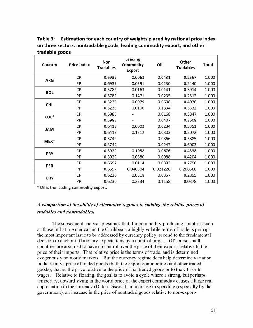
The key difference between the two price indices is that the weight of the commodity export should be far smaller in the CPI than in the PPI, and the weight of the import commodity the other way around. (If we take oil to be the only important source of terms of trade fluctuations on the import side, then this is of course less important for oil-exporting countries.) Table 3 reports the estimated weights that the countries’ CPI and PPI, respectively, place on each of three sectors: non-tradable goods, the leading commodity export (which in two cases is oil), and other tradables (which includes imports, exports other than the leading commodity export, and any other goods that are perfect substitutes for internationally traded goods). The methods for estimating the weights are described in an Appendix. As one might expect, Mexico (located next to the United States and having followed open trade policies for 20 years) shows the lowest share of goods that are not internationally traded, while Argentina (which is distant, and generally protectionist) registers the highest.

Also as one would expect, the share of the commodity export in the CPI is usually lower than its share in the PPI, sometimes far lower (Argentina, Bolivia, Jamaica, Peru and Uruguay). The two exceptions are Mexico and Paraguay. One can guess a possible explanation for Mexico: petroleum products are heavily subsidized in domestic consumption, and oil production has been declining in recent years. Paraguay is more of a puzzle. The explanation might simply be that it is one of the few Latin American countries that is not heavily specialized in the production and export of a small number of agricultural or mineral commodities.

21

Table 3:     Estimation for each country of weights placed by national price index on three sectors: nontradable goods, leading commodity export, and other tradable goods

Country  Price index Non 

Tradables 

Leading Commodity 

Export Oil 

Other Tradables 

Total 

ARG CPI  0.6939 0.0063 0.0431 0.2567  1.000

PPI  0.6939 0.0391 0.0230 0.2440  1.000

BOL CPI  0.5782 0.0163 0.0141 0.3914  1.000

PPI  0.5782 0.1471 0.0235 0.2512  1.000

CHL CPI  0.5235 0.0079 0.0608 0.4078  1.000

PPI  0.5235 0.0100 0.1334 0.3332  1.000

COL* CPI  0.5985  ‐‐  0.0168 0.3847  1.000

PPI  0.5985  ‐‐  0.0407 0.3608  1.000

JAM CPI  0.6413 0.0002 0.0234 0.3351  1.000

PPI  0.6413 0.1212 0.0303 0.2072  1.000

MEX* CPI  0.3749  ‐‐  0.0366 0.5885  1.000

PPI  0.3749  ‐‐  0.0247 0.6003  1.000

PRY CPI  0.3929 0.1058 0.0676 0.4338  1.000

PPI  0.3929 0.0880 0.0988 0.4204  1.000

PER CPI  0.6697 0.0114 0.0393 0.2796  1.000

PPI  0.6697 0.040504 0.021228 0.268568  1.000

URY CPI  0.6230 0.0518 0.0357 0.2895  1.000

PPI  0.6230 0.2234 0.1158 0.0378  1.000

* Oil is the leading commodity export.       

A comparison of the ability of alternative regimes to stabilize the relative prices of

tradables and nontradables.

The subsequent analysis presumes that, for commodity-producing countries such as those in Latin America and the Caribbean, a highly volatile terms of trade is perhaps the most important issue to be addressed by currency policy, second to the fundamental decision to anchor inflationary expectations by a nominal target. Of course small countries are assumed to have no control over the price of their exports relative to the price of their imports. That relative price is the terms of trade, and is determined exogenously on world markets. But the currency regime does help determine variation in the relative price of traded goods (both the export commodities and other traded goods), that is, the price relative to the price of nontraded goods or to the CPI or to wages. Relative to floating, the goal is to avoid a cycle where a strong, but perhaps temporary, upward swing in the world price of the export commodity causes a large real appreciation in the currency (Dutch Disease), an increase in spending (especially by the government), an increase in the price of nontraded goods relative to non-export-

22

commodity traded goods, a resultant shift of resources out of non-export-commodity traded goods, and a current account deficit -- all of which are painfully reversed when the world price of the export commodity goes back down. Relative to a fixed exchange rate or a CPI target, PEP and PPT might show an advantage, in accommodating fluctuations in the terms of trade. The goal is that a worsening in the terms of trade induces a weaker currency under PPT than it would under CPI-targeting, and therefore raises the price of non-commodity tradable goods relative to nontraded goods.

For those who wonder what is the market failure, the distortion at which monetary policy is aimed, the answer is that such price swings induce current account deficits and capital inflows that are not optimizing in the way standard theory says. Facets of the market failure could be excessively procyclical capital flows (including perhaps the absence of an effective international mechanism for handling default), or a political economy proclivity for governments to over-spend when the purchasing power of their revenues goes up (due to soaring commodity export tax receipts47), or speculative bubbles in real estate48 (as investors jump on the bandwagon of rising nontraded goods prices).

We will simulate the variability of the real prices of exports. It captures the unwanted side-effects of commodity booms (and busts): (1) the excessive swings in price signals that historically have induced labor and land to move into the production of commodities during the boom, only to reverse when the crash comes, and (2) the excessive swings in government revenue (royalties and corporate taxes on the commodity sector) in terms of purchasing power over local goods and services, which historically have tempted governments into pro-cyclical spending.

We do not model any of these real effects in the body of the paper. Rather we report implications of alternative regimes for movements in the key relative prices, a process that has the advantage of being largely model-free.49

More specifically, our analysis is guided by the assumption that the goals are, to

the extent possible, to minimize variability in the real price of commodity exports (to moderate resource swings into that sector when its world price temporarily rises) and to minimize variability in the real price of other traded goods (to moderate resource swings out of that sector). Again, these two objectives are second to the objective of anchoring inflationary expectations. But any nominal anchor can do that.50 We could choose to measure the relative price of traded goods in terms of non-traded goods, or in terms of wages. Instead we choose to measure the prices of these traded goods relative to the CPI. This comes pretty much to the same thing, because nontraded goods are the only other component in the CPI, other than traded goods (and the relative price of commodity exports versus other traded goods is deemed exogenous).

47 E.g., Lane and Tornell (1998). 48 Aizenman and Jinjarak (2008) find a strong positive association between current account deficits and the real increase in real estate prices 49 Appendix 2 models theoretically the effects of relative prices on output. One result there is that high sectoral elasticities of supply with respect to relative prices make it more likely that PEP dominates an exchange rate target. 50 Except to the extent that the variable chosen for nominal anchor is too likely when faced with shocks to lead to big distortions and thereby is not credible from the beginning. (This was the case with M1 targeting and, I would argue, would be also with strict CPI targeting.)

23

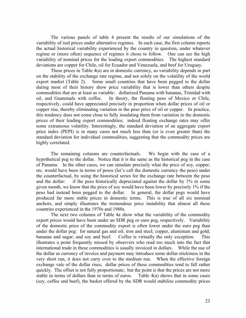
The various panels of table 4 present the results of our simulations of the

variability of real prices under alternative regimes. In each case, the first column reports the actual historical variability experienced by the country in question, under whatever regime or (more often) sequence of regimes it chose to follow. One can see the high variability of nominal prices for the leading export commodities. The highest standard deviations are copper for Chile, oil for Ecuador and Venezuela, and beef for Uruguay.

These prices in Table 4(a) are in domestic currency, so variability depends in part on the stability of the exchange rate regime, and not solely on the volatility of the world export market (Table 2). Some small countries that have been pegged to the dollar during most of their history show price variability that is lower than others despite commodities that are at least as variable: dollarized Panama with bananas, Trinidad with oil, and Guatemala with coffee. In theory, the floating peso of Mexico or Chile, respectively, could have appreciated precisely in proportion when dollar prices of oil or copper rise, thereby eliminating variation in the peso price of oil or copper. In practice, this tendency does not come close to fully insulating them from variation in the domestic prices of their leading export commodities; indeed floating exchange rates may offer some extraneous volatility. Interestingly, the standard deviation of an aggregate export price index (PEPI) is in many cases not much less than (or is even greater than) the standard deviation for individual commodities, suggesting that the commodity prices are highly correlated.

The remaining columns are counterfactuals. We begin with the case of a

hypothetical peg to the dollar. Notice that it is the same as the historical peg in the case of Panama. In the other cases, we can simulate precisely what the price of soy, copper, etc. would have been in terms of pesos (let’s call the domestic currency the peso) under the counterfactual, by using the historical series for the exchange rate between the peso and the dollar: if the peso historically depreciated against the dollar by 1% in some given month, we know that the price of soy would have been lower by precisely 1% if the peso had instead been pegged to the dollar. In general, the dollar pegs would have produced far more stable prices in domestic terms. This is true of all six nominal anchors, and simply illustrates the tremendous price instability that almost all these countries experienced in the 1970s and 1980s.

The next two columns of Table 4a show what the variability of the commodity export prices would have been under an SDR peg or euro peg, respectively. Variability of the domestic price of the commodity export is often lower under the euro peg than under the dollar peg: for natural gas and oil; iron and steel; copper, aluminum and gold; bananas and sugar; and soy and beef. Coffee is virtually the only exception. This illustrates a point frequently missed by observers who read too much into the fact that international trade in these commodities is usually invoiced in dollars. While the use of the dollar as currency of invoice and payment may introduce some dollar-stickiness in the very short run, it does not carry over to the medium run. When the effective foreign exchange vale of the dollar rises, dollar prices of these commodities tend to fall rather quickly. The offset is not fully proportionate; but the point is that the prices are not more stable in terms of dollars than in terms of euros. Table 4(a) shows that in some cases (soy, coffee and beef), the basket offered by the SDR would stabilize commodity prices

24

better than either the dollar or euro. Even in these cases, however, the difference is small, and this benefit would hardly seem worth giving up the simplicity of a single-currency peg.

After the currency peg columns comes PEP (Peg the Export Price). Variability

of the local-currency price of the leading export commodities is zero, by construction. The same is true of the full basket of exports in the case of PEPI (Peg the Export Price Index). Recall the essence of this regime: every time the dollar price of coffee falls by one per cent on world markets, the dollar value of the local currency falls by one per cent, leaving the local price of coffee unchanged. Nominal variability is far lower than under floating, and yet there is a clear nominal target to anchor inflation expectations. The best of both regimes. An overall judgment on the merits of the alternative regimes would have to be based on far more than this, of course. The column of zeros is a conspicuous “stacking of the deck” in favor of PEP and PEPI.

Table 4(b) reports the standard deviations of the percentage changes in the local-

currency commodity prices across the seven regimes. Again the currency pegs stabilize prices relative to the historical regime. (As one would expect, the reduction in volatility no longer looks quite so dramatic). The euro peg no longer dominates the dollar peg in terms of reducing local-currency price volatility; this is again what one would expect from a dollar-stickiness of commodity prices that pertains only to the short term.

Table 4(c) shows the standard deviation of real prices of the commodity exports,

across the seven regimes. Real is here defined in terms of the CPI, but we could just as well be looking at the relative price in terms of non-traded goods. This is the most important of the three measures of price volatility. It captures the unwanted side-effects of the commodity cycle: (1) the excessive swings in relative price signals that historically have induced resources to move in and out of the production of commodities, and (2) the excessive swings in real government revenue, which historically have yielded pro-cyclical spending.

The comparison of a PPI target with a CPI target, as an alternate possible

interpretation of inflation targeting, is the unique point of this study. The comparison in terms of ability to stabilize domestic prices of the principle export commodities appears in the last two columns of Tables 4(a) through 4(c). In most cases the standard deviation of the domestic price of the export commodity is lower under the PPI target than under the CPI target. In a few cases, it is less than half the size: Jamaica for aluminum and Uruguay for beef. The only times when variability is higher under the PPI target than under the CPI target is Mexico for oil and Paraguay for beef. The reason is immediately apparent: these were the only two countries where the export commodity strangely received a heavier estimated weight in the CPI than in the PPI; this cannot be the normal situation.

The one aspect of these tables that might be considered surprising is that, even though variability of the export commodity price tends to be lower under a PPI target than under a CPI target, under either form of inflation targeting it is generally substantially higher than under a currency peg, and often higher even than under the

25

various historical regimes. Perhaps this is an artifact of our approach that operationalizes inflation targeting as the precise hitting of the price index target, whether PPI or CPI. In practice this would be impossible to achieve. In our results, it is possible to achieve, but perhaps only at the expense of imposing wild fluctuations in the exchange rate to offset fully fluctuations in any one sector of the price index. Perhaps a more reasonable and realistic approach that allowed a band or cone for the targeted price index would yield more realistic results. In any case, the methods for implementing the CPI and PPI targets bear further examination in future research.

Stabilizing domestic prices of the export commodity is far from the only criterion

that should be considered in comparing alternative candidates for nominal anchor. Another one is stabilizing domestic prices of other tradable goods. A valid critique of PEP and PEPI is that it transfers uncertainty that would otherwise occur in the real price of commodity exports into uncertainty (which otherwise might not occur) in the real price of non-commodity exportables and importables. This critique is particularly relevant if diversification of the economy is valued.

In Table 5 we conduct simulations, under the same seven alternative regimes, for

the domestic prices of import goods. From the viewpoint of a small country, imports, like exports, have their prices determined on world markets. The biggest source of variability in the world price of LAC imports is bound to be oil price shocks (for the countries that are oil importers, rather than exporters). Tables 5(a) and 5(b) report the statistics on the variability of the nominal import price, measured in terms of levels or changes respectively. Again, the currency pegs cut nominal price variability substantially relative to the historical regime, but the euro peg and SDR peg both slightly dominate the dollar peg. The commodity peg (PEP) does indeed introduce some extra volatility into import prices, through exchange rate fluctuations, but the difference is not large. When we look at the level of local import prices, PPI targeting dominates CPI targeting. This supports the claim that the CPI target, if interpreted literally, forces the monetary authorities to tighten and appreciate in a perverse response to an increase in the world price of oil import (in the case of oil importers), and that the PPI target does not. When we look at changes in local import prices, the standard deviations under the CPI target and the PPI target are very close to each other, and close to the standard deviation under the currency pegs as well.

An attempt to construct anything like a comprehensive evaluation of regimes rooted in a theoretically established welfare criterion is far beyond the ambitions of this study. On the other hand, we cannot end the study with a state of affairs where the only horse race insures by construction that PEP wins.51 Instead, we conclude with an

51 In my first PEP papers, I pursued counterfactual simulations for the paths of exports, trade balances, and debt under alternative possible nominal anchors, for a wide variety of commodity-producing countries. There nothing was foreordained. But PEP did tend to product the result that in the late 1990s, when dollar commodity prices fell and many emerging market countries experienced currency crises, PEP automatically depreciated the currency, stimulated exports, and mitigated the debt problem – all without the need to abandon the pre-declared nominal anchor. LAC countries that appear in those simulations include Argentina (wheat); Bolivia, Ghana and Peru (gold), Brazil, Colombia, Costa Rica, El Salvador, Guatemala,

26

examination, in Table 6, of the implications of the alternative regimes for a simple objective function that is a weighted average of the standard deviation of the real price of commodity exports and the standard deviation of the real price of other tradables (just oil in this case, or another largest single import good: steel). In other words we pursue the logic that stabilizing the relative price of commodity exports is not much of an accomplishment if it comes at the expense of a corresponding destabilization of the relative price of other traded goods. The commodity price peg (PEP) is the winner in the competition to reduce relative price variability, by a fairly substantial margin when we look at the level of nominal prices (Table 6a) or the level of real prices (Table 6c), and by a smaller margin when we look at changes in nominal prices (Table 6b). The three currency pegs are again fairly similar to each other, showing less price variability than the historical regime but more than the commodity peg. In the central competition of the last two columns, the PPI target produces less relative price variability than the CPI target in most cases. Looking at real price variability in Table 6c, the only exception is Peru; the gain is substantial in the case of Jamaica and Uruguay, smaller for the others.  

Summary of Conclusions    What nominal variable is the best candidate for an anchor to monetary policy? Inflation Targeting, with its usual focus on the CPI, has over the past decade been the most popular choice among monetary economists, at least with respect to large industrialized countries. Developing countries differ in a number of relevant structural ways. They tend to be smaller, and thus to take prices of both imports and exports as given on world markets. They tend to be more vulnerable to supply shocks, particularly terms of trade shocks. This is especially true of countries that depend on the exports of agricultural and mineral commodities, a description that fits most countries in Latin America and the Caribbean. Inflation targeting – if interpreted literally and narrowly as stabilization of the CPI – has the undesirable property that it calls on the central bank to respond to an adverse supply shock by tightening monetary policy so much that the currency appreciates. It appears that Brazil, Chile and Peru do precisely that in response to oil price increases.

The regimes currently followed by the LAC countries are generally distributed across three categories: monetary targets, exchange rate targets, and inflation targets. These are official regimes; in practice many of the countries deviate from the declared targeting policy. Money-targeters, for example, let the monetary aggregates run well outside the proclaimed range, and inflation targeters intervene heavily in the foreign exchange market.

Honduras, Nicaragua, and Peru (coffee); Chile (copper); Colombia, Ecuador, Mexico and Venezuela (oil); Bolivia and Peru (slver); and Jamaica and Surinam (aluminum). Of course commodity composition of exports evolves over time; some of these associations may not be as relevant looking forward.

27

This study has focused on a comparison of exchange rate pegs and inflation targets, but has also highlighted a new untried set of proposals. These proposals call for targeting prices of whatever commodities are the important exports of the country in question. The proposals range from the most exotic to the more down-to-earth. The most exotic is the idea of Pegging the Export Price (PEP): Bolivia would fix the dollar price of the sole to the dollar price of natural gas; Chile would intervene to keep the value of its peso constant in terms of copper; Jamaica would peg its dollar to aluminum; and Uruguay would peg its peso to the price of beef. A less radical version that takes export diversification into account is Peg the Export Price Index (PEPI), which aims to stabilize a basket, perhaps a comprehensive basket, of export prices in terms of the local currency. Finally, the version that sounds the most reassuring and reasonable would be Product Price Targeting (PPT): to target in place of the CPI the Producer Price Index or a specially constructed index of product prices weighted by shares in output. All three versions dominate a policy of targeting the CPI, to the extent that terms of trade shocks are important, as they are for the LAC countries. All three have the desirable property that the currency appreciates when prices for exports go up on world markets and depreciates when they go down; the CPI does not have that desirable property.

In addition, if inflation targeting is interpreted strictly as a commitment to the CPI, it has the undesirable property that the currency appreciates when the prices of imports such as oil go up on world markets, and depreciates when they go down; PEP, PEPI and PPT targeting don’t have this undesirable property. Table 1 provides a preliminary indication that ever since 1999, when Brazil and Chile switched from exchange rate targeting to CPI targeting, they have experienced a higher correlation between the dollar price of their currencies and the dollar price of oil imports. This suggests that, language about core CPI notwithstanding, the monetary authorities in these two countries have found it necessary to respond to the oil price increases of the last decade by contracting monetary policy enough to appreciate their currencies. The production-based price targets would not have this problem. The heart of the analysis is the comparison of seven alternative nominal targets according to how they would affect the variability of the real prices of tradables: commodity exports in Table 4, imports in Table 5, and both together in Table 6. Some conclusions are very predictable. First, according to the simulations the currency anchors offer far more price stability than does the historical reality, because our counterfactual was that the countries had the benefits of the anchor from before the beginning of the sample. An interesting extension would be a simulation in which the countries switched to their nominal anchors sometime in the 1990s, requiring a gradual adjustment of nontraded goods prices. Second, PEP perfectly stabilizes the domestic price of export commodities, by construction. The more interesting findings are the comparison of a CPI target and a Product Price target as alternative interpretations of inflation targeting. The results show that the PPI target generally delivers more stability in the prices of traded goods, especially the export commodity. This is a natural consequence of the larger weight on commodity exports in the PPI than in the CPI. (The major exception to the regime ranking is Mexico, a consequence of the anomalous larger weight on oil in the CPI than in the PPI, according to our numbers.) Perhaps surprisingly, both the CPI target and the PPI target deliver more relative price variability than any of the three exchange rate targets (dollar,

28

euro and SDR). More research is clearly needed here, to see if the estimation of the sectoral weights and the price series can be improved, and to make the comparison more realistic by allowing the CPI and Product Price Index to fall within a target range rather than requiring the central bank to hit a target precisely.

29

References Aizenman, J. and Y. Jinjarak, 2008. “Current Account Patterns and National Real Estate Markets,” NBER

Working Paper No. 13921, April.

Arnone, Marco, Bernard Laurens and Jean-François Segalotto , 2006, “Measures of Central Bank Autonomy: Empirical Evidence for OECD, Developing, and Emerging Market Economies,” October, IMF Working Paper No. 06/228.

Bayoumi, Tamim, and Barry Eichengreen 1994, ”One Money or Many? Analyzing the Prospects for

Monetary Unification in Various Parts of the World,” Studies in International Finance No. 76 (September), Princeton University Press.

Bean, Charles, 1983, “Targeting Nominal Income: An Appraisal,” Economic Journal 93, Dec., 806-819. Berg, A., E Borensztein, P Mauro, 2003, “Monetary Regime Options for Latin America,” Finance and

Development, September, pp 24-27 Bernanke, Ben, Thomas Laubach, Frederic Mishkin, and Adam Posen, 1999, Inflation Targeting: Lessons

from the International Experience, Princeton University Press: Princeton NJ. Blanchard, Olivier, 2005, “Fiscal Dominance and Inflation Targeting: Lessons from Brazil,” Chapter 2, in

Francesco Giavazzi, Ilan Goldfajn, and Santiago Herrera, editors, Inflation Targeting, Debt, and the Brazilian Experience, 1999 to 2003 (MIT Press: Cambridge), 49-80. MIT Department of Economics Working Paper No. 04-13.

Broda, Christian, 2004, "Terms of Trade and Exchange Rate Regimes in Developing Countries," Journal of

International Economics, 63(1), pp. 31-58. Caballero, Ricardo 2000., “Macroeconomic Volatility in Latin America: A Conceptual Framework and

Three Case Studies,” Economia 1.1 (LACEA) 31-88. Caballero, Ricardo and Arvind Krishnamurthy, 2003, “Inflation Targeting and Sudden Stops,” NBER

Working Paper No. 9599. Calvo, Guillermo, Leonardo Leiderman and Carmen Reinhart, 1993, “Capital Inflows and Real Exchange

Rate Appreciation in Latin America: The Role of External Factors,” IMF Staff papers, 40, no. 1, March.

Collins, Susan, 1996, “On becoming more flexible: Exchange rate regimes in Latin America and the Caribbean,” Journal of Development Economics, vol. 51, issue 1, pages 117-138.

Cooper, Richard, 1985, “The Gold Standard: Historical Facts and Future Prospects,” Brookings Papers on

Economic Activity, 1, 1-45. Cukierman, Alex, Geoffrey Miller and Bilin Neyapti, 2002 “Central bank reform, liberalization and

inflation in transition economies—an international perspective,” Journal of Monetary Economics v, March, Pages 237-264.

Debelle, Guy, 2001, “The Case for Inflation Targeting in East Asian Countries,” Future Directions for

Monetary Policies in East Asia, David Gruen and John Simon, eds. (Reserve Bank of Australia).

30

Edwards, Sebastian, and Eduardo Levy Yeyati, 2005, “Flexible Exchange Rates as Shock Absorbers,”

European Economic Review, Vol. 49, Issue 8, November, pp. 2079-05. NBER Working Paper 9867. Edwards, Sebastian. 2006, “The Relationship Between Exchange Rates and Inflation Targeting Revisited,”

Banco de Chile Annual Research Conferences, Santiago, October 2005, NBER WP No. 12163, April. Eichengreen, Barry, 1985, The Gold Standard in Theory and History (New York: Methuen). Engel, Charles, 1999, “Accounting for U.S. Real Exchange Rate Changes.” Journal of Political Economy, vol.

107, no. 3, June, pp. 507-538. Feldstein, Martin, and James Stock, 1994, “The Use of a Monetary Aggregate to Target Nominal GDP,” in

Monetary Policy, edited by N. Greg Mankiw (Chicago: University of Chicago Press), pp 7-70. Foresti, Pasquale, 2007, “Is Latin America an Optimal Currency Area? Evidence from a Structural Vector

Auto-regression Analysis,” April, MPRA paper 2961, http://mpra.ub.uni-muenchen.de/2961/1/MPRA_paper_2961.pdf .

Fraga, Armino, Ilan Goldafjn and Andre Minella, 2003, “Inflation Targeting in Emerging Market

Economies,” NBER Macro Annual 2003, edited by Ken Rogoff and Mark Gertler (MIT Press: Cambridge). NBER WP no. 10019.

Frankel, Jeffrey, 1985, "The Stabilizing Properties of a Nominal GNP Rule," Journal of Money, Credit and

Banking 27, no. 2, May, 318-334. Frankel, Jeffrey, 2002, “Should Gold-Exporters Peg Their Currencies to Gold?” Research Study No. 29

(World Gold Council: London). Frankel, Jeffrey, 2003, “A Proposed Monetary Regime for Small Commodity Exporters: Peg the Export

Price (PEP),” International Finance (Blackwill Publishers), 6, no. 1, Spring, 61-88. Frankel, Jeffrey, 2004, “Experience of and Lessons from Exchange Rate Regimes in Emerging

Economies,” in Monetary and Financial Integration in East Asia: The Way Ahead, Asian Development Bank (Palgrave Macmillan Press, New York ), vol. 2, 91-138.

Frankel, Jeffrey, 2005, “Peg the Export Price Index: A Proposed Monetary Regime for Small Countries,”

Journal of Policy Modeling, vol. 27, no.4, June, pp. 495-508. Frankel, Jeffrey, 2010, “Are Bilateral Remittances Countercyclical?” forthcoming, Open Economies Review.

NBER WP No. 15419, 2009. Frankel, Jeffrey, and Ayako Saiki, 2002. “A Proposal to Anchor Monetary Policy by the Price of the Export

Commodity,” Journal of Economic Integration, September, 17, no. 3: 417-448. Frankel, Jeffrey, Ben Smit, and Federico Sturzenegger, 2008, "South Africa: Macroeconomic Challenges after

a Decade of Success," Economics of Transition 16, no. 4, 639-677 (Blackwell). Gavin, Michael, Ricardo Hausmann and Leonardo Leiderman , 1996, “Macroeconomics of Capital Flows to

Latin America: Experience and Policy Issues,” Inter-American Development Bank, Research Department Working Paper no. 4012.

Gavin, Michael, Ricardo Hausmann, Roberto Perotti and Ernesto Talvi, 1997, “Managing Fiscal Policy in Latin

America and the Caribbean: Volatility, Procyclicality, and Limited Creditworthiness,” Revista del Banco Central de Venezuela, vol. XI (1). Inter-American Development Bank, RES WP 4032, 1996.

31

Giavazzi, Francesco, Ilan Goldfajn, and Santiago Herrera, 2005, “Overview: Lessons from Brazil,” in Inflation Targeting, Debt, and the Brazilian Experience, 1999 to 2003 (MIT Press: Cambridge).

Graham, Benjamin, 1937, Storage and Stability (New York: McGraw Hill). Gutiérez, Eva, 2003, “Inflation Performance and Constitutional Central Bank Independence: Evidence from

Latin America and the Caribbean,” IMF WP/03/53, March. Hall, Robert, 1985, “Monetary Policy with an Elastic Price Standard,” Price Stability and Public Policy

(Federal Reserve Bank of Kansas City). Hall, Robert, 1982, “Explorations in the Gold Standard and Related Policies for Stabilizing the Dollar,” in

Hall, ed., Inflation (Chicago: University of Chicago Press), 111-122. Hausmann, Ricardo, and Roberto Rigobon, 2003, “An Alternative Interpretation of the ‘Resource Curse’:

Theory and Policy Implications,” NBER WP no. 9424, January. Jácome, Luis I., 2001, “Legal Central Bank Independence and Inflation in Latin America During the

1990s,” International Monetary Fund Working Paper No. 01/212, December. Jácome, Luis and Francisco Vázquez, 2008 , “Is there any link between legal central bank independence

and inflation? Evidence from Latin America and the Caribbean,” Paolo Baffi Centre Research Paper No. 2008-07, March.

Junguito, Roberto, and Hernando Vargas, 1996,“Central Bank Independence and Foreign Exchange

Policies in Latin America,” Banco de la Republica de Colombia, Borradores de Economia series, no. 046, Bogota, Feb.

Kaminsky, Graciela, Carmen Reinhart and Carlos Vegh, 2005."When It Rains, It Pours: Procyclical Capital

Flows and Macroeconomic Policies," NBER Macroeconomics Annual 2004, Vol. 19, pages 11-82. Keynes, John Maynard , 1938, “The Policy of Government Storage of Foodstuffs and Raw Materials,”

Economic Journal, September. Kiguel, Miguel and Nissan Liviatan, 1992, “The Business Cycle Associated with Exchange Rate-Based

Stabilizations,” World Bank Economic Review, Vol 6, Number 2 pp. 279-305. Lake, Lisa, 2006, “Remittances and the Jamaican Economy: From Fundamentals to Effective Policy

Recommendations.” MPA/ID Second Year Policy Analysis, Harvard Kennedy School. Lane, Philip and Aaron Tornell, 1998. “Voracity and Growth,” NBER WP 6498; published as "Voracity

and Growth in Discrete Time", EL, Vol. 62, no. 1 (January 1999): 139-145. Laxton, Douglas, and Paolo Pesenti, 2003, “Monetary Rules for Small, Open, Emerging Economies,”

NBER WP No. 9568. Levy Yeyati, Eduardo, and Federico Sturzennegger, 2000, “The Euro and Latin America : Is EMU a

Blueprint for Mercosur?” American Journal of Economics, No. 110 , pp. 63-99. Levy-Yeyati, Eduardo, and Federico Sturzenegger, 2003, “To Float or to Trail: Evidence on the Impact of

Exchange Rate Regimes on Growth,” American Economic Review, 93, No. 4, Sept., pp. 1173-93. Loayza, Norman, Pablo Fajnzylber, César Calderón, 2005, “Economic Growth in Latin America and the

Caribbean: Stylized Facts, Explanations and Forecasts” (World Bank).

32

Mas, Ignacio, 1995, “Central Bank Independence: A Critical View from a Developing Country Perspective,” World Development, Vol. 23, Issue 10, October, pages 1639-1652.

Masson, Paul, Miguel Savastano and Sunil Sharma, 1997, “The Scope for Inflation Targeting in

Developing Countries,” IMF WP/97/130, October. McKibbin, W., and K. Singh, 2003, “Issues in the Choice of a Monetary Regime for India,” Australian

National University, May 2000. Brookings Discussion Papers in International Economics No. 154, September 2003.

McKinnon, Ronald, 1963, “Optimum Currency Areas,” American Economic Review, vol.53, September,

pp. 657-65. Mendoza, Enrique and Marco Terrones, 2008, “An Anatomy of Credit Booms: Evidence from Macro

Aggregates and Micro Data,” NBER Working Paper No. 14049, May. Mishkin, Frederic, 2000, “Inflation targeting in emerging-market countries,” American Economic Review. Mishkin, Frederic, 2008, “Can Inflation Targeting Work in Emerging Market Countries?” in Money,

Crises, and Transition: Essays in Honor of Guillermo Calvo, edited by Carmen Reinhart, Carlos Vegh and Andres Velasco . NBER WP 10646, 2004.

Mishkin, Frederic, and Miguel Savastano, 2002, “Monetary Policy Strategies for Emerging Market

Countries: Lessons from Latin America,” Comparative Economic Studies. Mundell, Robert, 1961, “The Theory of Optimal Currency Areas,” American Economic Review 51,

November, 509-517. Obstfeld, Maurice, 1986, “Rational and Self-Fulfilling Balance-of-Payments Crises,” American Economic

Review, vol. 76, no. 1, March 72-81. Perry, Guillermo, 2009, “Beyond Lending: How Multilateral Banks Can Help Developing Countries

Manage Volatility,” Center for Global Development, Washington, DC. Reinhart, Carmen, and Vincent Reinhart, 2009, “Capital Flow Bonanzas: An Encompassing View of the

Past and Present,” in J.Frankel and C.Pissarides, eds., NBER International Seminar in Macroeconomics 2008 (Chicago: University of Chicago Press).

Rogoff, Kenneth, 1985, “The Optimal Degree of Commitment to an Intermediate Monetary Target,” Quarterly

Journal of Economics 100, November: 1169-89. Rose, Andrew K., 2000, “One Money, One Market: Estimating the Effect of Common Currencies on

Trade,” Economic Policy, Vol. 15, No. 30, April, pp. 8–45 Savastano, Miguel, 2000, “Inflation Targeting in Non-Industrial Countries,” IMF Research Bulletin 1, no. Svensson, Lars, 1995, “The Swedish Experience of an Inflation Target,” in Inflation Targets, edited by Leo

Leiderman and Lars Svensson (Centre for Economic Policy Research: London). Taylor, Alan, 2002, "A Century Of Purchasing-Power Parity," Review of Economics and Statistics, vol. 84

February, 139-150. Taylor , John. 1985. “What Would Nominal GNP Targeting Do to the Business Cycle?” Carnegie-

Rochester Conference Series on Public Policy 22: 61-84.

33

Tobin, James. 1980. “Stabilization Policy Ten Years After,” Brookings Papers on Economic Activity 1: 19-72.

Truman, Edwin, 2003, Inflation Targeting in the World Economy, Institute for International Economics,

Washington DC. Vargas, Hernando, 2005, “Exchange Rate Policy and Inflation Targeting in Colombia,” Banco de la

República, Colombia, September. West, Kenneth, 1986, “Targeting Nominal Income: A Note,” Economic Journal, 96, Dec., 1077-1083.

34

Table 4: Variability of Export Prices under Alternative Currency Regimes (a) Standard Deviation of Level of Nominal Export Prices 

Historical 

RegimeDollar Peg SDR Peg Euro Peg

Comm. 

PegCPI Target PPI Target

ARG Soy 1.927 0.278 0.251 0.265 0.000 1.271 1.037

ARG Basket 1.966 0.331 0.281 0.260 0.000  ‐‐  ‐‐

ARG PEPI 2.433 0.104 0.064 0.093 0.000  ‐‐  ‐‐

BOL Nat. Gas 1.997 0.627 0.591 0.594 0.000 0.907 0.584

BOL PEPI 1.685 0.581 0.594 0.581 0.000  ‐‐  ‐‐

BRA Steel 2.240 0.590 0.495 0.418 0.000  ‐‐  ‐‐

BRA Iron Ore 2.180 0.460 0.388 0.333 0.000  ‐‐  ‐‐

BRA Basket 2.186 0.415 0.333 0.281 0.000  ‐‐  ‐‐

BRA PEPI 2.601 0.405 0.320 0.236 0.000  ‐‐  ‐‐

CHL Copper 3.178 0.408 0.342 0.311 0.000 1.113 0.952

COL Oil 2.315 0.759 0.697 0.623 0.000 1.123 0.974

COL Coffee 1.752 0.479 0.494 0.504 0.000  ‐‐  ‐‐

COL PEPI 0.553 0.186 0.155 0.166 0.000  ‐‐  ‐‐

CRI Bananas 1.930 0.442 0.372 0.306 0.000  ‐‐  ‐‐

CRI Coffee 1.577 0.479 0.494 0.504 0.000  ‐‐  ‐‐

ECU Oil 3.288 0.759 0.697 0.623 0.000  ‐‐  ‐‐

ECU PEPI 3.044 0.491 0.457 0.426 0.000  ‐‐  ‐‐

GTM Coffee 0.910 0.479 0.494 0.504 0.000  ‐‐  ‐‐

GUY Sugar 2.059 0.475 0.433 0.436 0.000  ‐‐  ‐‐

GUY PEPI 1.914 0.404 0.372 0.325 0.000  ‐‐  ‐‐

HND Coffee 0.971 0.479 0.494 0.504 0.000  ‐‐  ‐‐

HND PEPI 0.937 0.277 0.305 0.334 0.000  ‐‐  ‐‐

JAM Aluminium 1.959 0.418 0.361 0.303 0.000 1.222 0.565

JAM PEPI 1.579 0.167 0.155 0.199 0.000  ‐‐  ‐‐

MEX Oil 3.238 0.759 0.697 0.623 0.000 0.975 1.030

NIC Coffee 2.185 0.479 0.494 0.504 0.000  ‐‐  ‐‐

PAN Bananas 0.442 0.442 0.372 0.306 0.000  ‐‐  ‐‐

PER Copper 1.923 0.408 0.342 0.311 0.000 0.671 0.688

PER Gold 1.909 0.708 0.638 0.536 0.000  ‐‐  ‐‐

PER PEPI 1.951 0.378 0.320 0.288 0.000  ‐‐  ‐‐

PRY Beef 1.623 0.230 0.206 0.224 0.000 0.694 0.715

SLV Coffee 0.670 0.479 0.494 0.504 0.000  ‐‐  ‐‐

TTO Nat. Gas 0.929 0.627 0.591 0.594 0.000  ‐‐  ‐‐

URY Beef 3.641 0.230 0.206 0.224 0.000 0.893 0.410

VEN Oil 2.931 0.759 0.697 0.623 0.000  ‐‐  ‐‐

Nominal Export Prices

35

(b) Standard Deviation of First Difference of Nominal Export Prices 

Historical 

RegimeDollar Peg SDR Peg Euro Peg

Comm. 

PegCPI Target PPI Target

ARG Soy 0.201 0.067 0.068 0.073 0.000 0.061 0.041

ARG Basket 0.179 0.051 0.052 0.059 0.000  ‐‐  ‐‐

ARG PEPI 1.798 1.385 1.299 1.570 0.000  ‐‐  ‐‐

BOL Nat. Gas 0.417 0.106 0.105 0.106 0.000 0.102 0.071

BOL PEPI 0.204 0.055 0.059 0.066 0.000  ‐‐  ‐‐

BRA Steel 0.149 0.090 0.091 0.095 0.000  ‐‐  ‐‐

BRA Iron Ore 0.123 0.050 0.054 0.059 0.000  ‐‐  ‐‐

BRA Basket 0.127 0.046 0.048 0.055 0.000  ‐‐  ‐‐

BRA PEPI 0.969 0.097 0.101 0.131 0.000  ‐‐  ‐‐

CHL Copper 0.122 0.078 0.076 0.078 0.000 0.070 0.073

COL Oil 0.078 0.075 0.076 0.080 0.000 0.067 0.059

COL Coffee 0.083 0.083 0.085 0.090 0.000  ‐‐  ‐‐

COL PEPI 0.036 0.033 0.033 0.042 0.000  ‐‐  ‐‐

CRI Bananas 0.159 0.154 0.156 0.158 0.000  ‐‐  ‐‐

CRI Coffee 0.096 0.083 0.085 0.090 0.000  ‐‐  ‐‐

ECU Oil 0.089 0.075 0.076 0.080 0.000  ‐‐  ‐‐

ECU PEPI 0.177 0.170 0.171 0.174 0.000  ‐‐  ‐‐

GTM Coffee 0.092 0.083 0.085 0.090 0.000  ‐‐  ‐‐

GUY Sugar 0.135 0.105 0.105 0.108 0.000  ‐‐  ‐‐

GUY PEPI 0.379 0.217 0.217 0.224 0.000  ‐‐  ‐‐

HND Coffee 0.109 0.083 0.085 0.090 0.000  ‐‐  ‐‐

HND PEPI 0.282 0.259 0.260 0.267 0.000  ‐‐  ‐‐

JAM Aluminium 0.065 0.049 0.052 0.059 0.000 0.048 0.018

JAM PEPI 0.192 0.128 0.124 0.150 0.000  ‐‐  ‐‐

MEX Oil 0.090 0.075 0.076 0.080 0.000 0.064 0.067

NIC Coffee 0.184 0.083 0.085 0.090 0.000  ‐‐  ‐‐

PAN Bananas 0.154 0.154 0.156 0.158 0.000  ‐‐  ‐‐

PER Copper 0.168 0.078 0.076 0.078 0.000 0.076 0.076

PER Gold 0.158 0.051 0.049 0.051 0.000  ‐‐  ‐‐

PER PEPI 0.218 0.136 0.138 0.142 0.000  ‐‐  ‐‐

PRY Beef 0.065 0.044 0.047 0.055 0.000 0.027 0.031

SLV Coffee 0.096 0.083 0.085 0.090 0.000  ‐‐  ‐‐

TTO Nat. Gas 0.109 0.106 0.105 0.106 0.000  ‐‐  ‐‐

URY Beef 0.076 0.044 0.047 0.055 0.000 0.028 0.022

VEN Oil 0.116 0.075 0.076 0.080 0.000  ‐‐  ‐‐

First Difference of Nominal Export Prices

 

36

(c) Standard Deviation of Level of Real Export Prices 

Historical 

RegimeDollar Peg SDR Peg Euro Peg

Comm. 

PegCPI Target PPI Target

ARG Soy 0.561 0.497 0.523 0.483 0.000 0.858 0.767

ARG Basket 0.578 0.418 0.443 0.408 0.000  ‐‐  ‐‐

ARG PEPI 0.312 0.140 0.128 0.110 0.000  ‐‐  ‐‐

BOL Nat. Gas 0.556 0.402 0.431 0.483 0.000 0.438 0.322

BOL PEPI 0.523 0.616 0.650 0.638 0.000  ‐‐  ‐‐

BRA Steel 0.496 0.427 0.403 0.363 0.000  ‐‐  ‐‐

BRA Iron Ore 0.412 0.332 0.353 0.335 0.000  ‐‐  ‐‐

BRA Basket 0.355 0.360 0.370 0.336 0.000  ‐‐  ‐‐

BRA PEPI 0.403 0.191 0.220 0.206 0.000  ‐‐  ‐‐

CHL Copper 0.418 0.485 0.496 0.451 0.000 0.909 0.815

COL Oil 0.456 0.485 0.482 0.490 0.000 1.123 0.974

COL Coffee 0.528 0.690 0.717 0.680 0.000  ‐‐  ‐‐

COL PEPI 0.121 0.153 0.128 0.138 0.000  ‐‐  ‐‐

CRI Bananas 0.273 0.252 0.283 0.281 0.000  ‐‐  ‐‐

CRI Coffee 0.566 0.690 0.717 0.680 0.000  ‐‐  ‐‐

ECU Oil 0.456 0.485 0.482 0.490 0.000  ‐‐  ‐‐

ECU PEPI 0.302 0.381 0.406 0.404 0.000  ‐‐  ‐‐

GTM Coffee 0.603 0.690 0.717 0.680 0.000

GUY Sugar 0.823 0.677 0.676 0.624 0.000  ‐‐  ‐‐

GUY PEPI 0.692 0.375 0.400 0.396 0.000  ‐‐  ‐‐

HND Coffee 0.594 0.690 0.717 0.680 0.000  ‐‐  ‐‐

HND PEPI 0.414 0.507 0.525 0.491 0.000  ‐‐  ‐‐

JAM Aluminium 0.272 0.281 0.321 0.316 0.000 1.222 0.565

JAM PEPI 0.239 0.363 0.383 0.356 0.000  ‐‐  ‐‐

MEX Oil 0.479 0.485 0.482 0.490 0.000 0.975 1.030

NIC Coffee 0.482 0.690 0.717 0.680 0.000  ‐‐  ‐‐

PAN Bananas 0.210 0.252 0.283 0.281 0.000  ‐‐  ‐‐

PER Copper 0.408 0.485 0.496 0.451 0.000 0.437 0.434

PER Gold 0.250 0.440 0.422 0.406 0.000  ‐‐  ‐‐

PER PEPI 0.338 0.349 0.345 0.308 0.000  ‐‐  ‐‐

PRY Beef 0.312 0.425 0.468 0.441 0.000 0.694 0.715

SLV Coffee 0.945 0.690 0.717 0.680 0.000  ‐‐  ‐‐

TTO Nat. Gas 0.357 0.402 0.431 0.483 0.000  ‐‐  ‐‐

URY Beef 0.494 0.425 0.468 0.441 0.000 0.893 0.410

VEN Oil 0.429 0.485 0.482 0.490 0.000  ‐‐  ‐‐

Real Export Prices

37

Table 5: Variability of Import Prices under Alternative Currency Regimes * (a) Standard Deviation of  Level of Nominal Import Prices 

Historical 

Regime

Dollar 

PegSDR Peg Euro Peg

Comm. 

Peg

CPI 

Target

PPI 

Target

ARG Oil 2.242 0.759 0.697 0.623 0.647 0.886 0.740

ARG Steel 2.134 0.527 0.428 0.349 0.428 0.982 0.749

BOL Oil 1.939 0.759 0.697 0.623 0.358 0.771 0.659

BOL Steel 2.052 0.527 0.428 0.349 0.478 0.586 0.501

BRA Oil 2.290 0.759 0.697 0.623 0.538  ‐‐  ‐‐

CHL Oil 3.636 0.759 0.697 0.623 0.597 0.771 0.578

CHL Steel 3.372 0.527 0.428 0.349 0.345 0.817 0.677

COL Steel 2.166 0.527 0.428 0.349 0.538 1.193 1.073

CRI Oil 2.142 0.759 0.697 0.623 0.484  ‐‐  ‐‐

CRI Steel 1.967 0.527 0.428 0.349 0.405  ‐‐  ‐‐

ECU Steel 3.187 0.527 0.428 0.349 0.538  ‐‐  ‐‐

GTM Oil 1.444 0.759 0.697 0.623 0.765  ‐‐  ‐‐

GTM Steel 1.323 0.527 0.428 0.349 0.669  ‐‐  ‐‐

GUY Oil 2.463 0.759 0.697 0.623 0.766  ‐‐  ‐‐

GUY Steel 2.367 0.527 0.428 0.349 0.581  ‐‐  ‐‐

HND Oil 1.504 0.759 0.697 0.623 0.765  ‐‐  ‐‐

HND Steel 1.370 0.527 0.428 0.349 0.669  ‐‐  ‐‐

JAM Oil 2.207 0.759 0.697 0.623 0.452 1.074 0.777

MEX Steel 3.125 0.527 0.428 0.349 0.538 1.050 1.094

NIC Oil 2.389 0.759 0.697 0.623 0.765  ‐‐  ‐‐

NIC Steel 2.338 0.527 0.428 0.349 0.669  ‐‐  ‐‐

PAN Oil 0.759 0.759 0.697 0.623 0.484  ‐‐  ‐‐

PAN Steel 0.527 0.527 0.428 0.349 0.405  ‐‐  ‐‐

PER Oil 2.115 0.759 0.697 0.623 0.597 0.792 0.718

PER Steel 2.059 0.527 0.428 0.349 0.345 0.803 0.613

PRY Oil 2.049 0.759 0.697 0.623 0.625 0.792 0.718

PRY Steel 1.939 0.527 0.428 0.349 0.444 0.803 0.613

SLV Oil 1.153 0.759 0.697 0.623 0.765  ‐‐  ‐‐

SLV Steel 1.012 0.527 0.428 0.349 0.669  ‐‐  ‐‐

TTO Oil 1.089 0.759 0.697 0.623 0.358  ‐‐  ‐‐

TTO Steel 0.914 0.527 0.428 0.349 0.478  ‐‐  ‐‐

URY Oil 3.966 0.759 0.697 0.623 0.625 0.693 0.639

URY Steel 3.896 0.527 0.428 0.349 0.444 0.562 0.408

VEN Steel 2.835 0.527 0.428 0.349 0.538  ‐‐  ‐‐

Nominal Import Prices

* Commodity peg refers to regime where the country's currency is pegged to the price of the leading commodity export.

38

(b) Standard Deviation of First Difference of Nominal Import Prices 

Historical 

Regime

Dollar 

PegSDR Peg Euro Peg

Comm. 

PegCPI Target PPI Target

ARG Oil 0.197 0.075 0.076 0.080 0.099 0.058 0.076

ARG Steel 0.209 0.106 0.105 0.107 0.112 0.105 0.106

BOL Oil 0.218 0.075 0.076 0.080 0.183 0.207 0.137

BOL Steel 0.223 0.106 0.105 0.107 0.261 0.287 0.205

BRA Oil 0.140 0.075 0.076 0.080 0.111  ‐‐  ‐‐

CHL Oil 0.124 0.075 0.076 0.080 0.097 0.062 0.050

CHL Steel 0.143 0.106 0.105 0.107 0.125 0.109 0.110

COL Steel 0.104 0.106 0.105 0.107 0.125 0.106 0.106

CRI Oil 0.087 0.075 0.076 0.080 0.174  ‐‐  ‐‐

CRI Steel 0.110 0.106 0.105 0.107 0.189  ‐‐  ‐‐

ECU Steel 0.116 0.106 0.105 0.107 0.125  ‐‐  ‐‐

GTM Oil 0.086 0.075 0.076 0.080 0.110  ‐‐  ‐‐

GTM Steel 0.116 0.106 0.105 0.107 0.134  ‐‐  ‐‐

GUY Oil 0.112 0.075 0.076 0.080 0.124  ‐‐  ‐‐

GUY Steel 0.135 0.106 0.105 0.107 0.151  ‐‐  ‐‐

HND Oil 0.103 0.075 0.076 0.080 0.110  ‐‐  ‐‐

HND Steel 0.128 0.106 0.105 0.107 0.134  ‐‐  ‐‐

JAM Oil 0.085 0.075 0.076 0.080 0.077 0.063 0.079

MEX Steel 0.117 0.106 0.105 0.107 0.125 0.106 0.106

NIC Oil 0.182 0.075 0.076 0.080 0.110  ‐‐  ‐‐

NIC Steel 0.194 0.106 0.105 0.107 0.134  ‐‐  ‐‐

PAN Oil 0.075 0.075 0.076 0.080 0.174  ‐‐  ‐‐

PAN Steel 0.106 0.106 0.105 0.107 0.189  ‐‐  ‐‐

PER Oil 0.191 0.075 0.076 0.080 0.097 0.068 0.086

PER Steel 0.189 0.106 0.105 0.107 0.125 0.111 0.117

PRY Oil 0.088 0.075 0.076 0.080 0.085 0.068 0.086

PRY Steel 0.114 0.106 0.105 0.107 0.116 0.111 0.117

SLV Oil 0.080 0.075 0.076 0.080 0.110  ‐‐  ‐‐

SLV Steel 0.111 0.106 0.105 0.107 0.134  ‐‐  ‐‐

TTO Oil 0.078 0.075 0.076 0.080 0.117  ‐‐  ‐‐

TTO Steel 0.110 0.106 0.105 0.107 0.145  ‐‐  ‐‐

URY Oil 0.284 0.075 0.076 0.080 0.085 0.070 0.068

URY Steel 0.196 0.106 0.105 0.107 0.116 0.109 0.110

VEN Steel 0.137 0.106 0.105 0.107 0.125  ‐‐  ‐‐

First Difference of Nominal Import Prices

* Commodity peg refers to regime where the country's exchange rate is pegged to the price of the leading commodity export.

39

(c) Standard Deviation of Level of Real Import Prices 

Historical 

Regime

Dollar 

PegSDR Peg Euro Peg

Comm. 

PegCPI Target PPI Target

ARG Oil 0.760 0.485 0.482 0.490 0.482 0.654 0.591

ARG Steel 0.684 0.380 0.359 0.315 0.378 0.646 0.567

BOL Oil 0.520 0.485 0.482 0.490 0.277 0.539 0.574

BOL Steel 0.483 0.380 0.359 0.315 0.435 0.523 0.452

BRA Oil 0.549 0.485 0.482 0.490 0.374  ‐‐  ‐‐

CHL Oil 0.601 0.485 0.482 0.490 0.597 0.771 0.578

CHL Steel 0.478 0.380 0.359 0.315 0.345 0.817 0.677

COL Steel 0.368 0.380 0.359 0.315 0.538 1.193 1.073

CRI Oil 0.568 0.485 0.482 0.490 0.484  ‐‐  ‐‐

CRI Steel 0.330 0.380 0.359 0.315 0.405  ‐‐  ‐‐

ECU Steel 0.393 0.380 0.359 0.315 0.538  ‐‐  ‐‐

GTM Oil 0.416 0.485 0.482 0.490 0.765  ‐‐  ‐‐

GTM Steel 0.368 0.380 0.359 0.315 0.669  ‐‐  ‐‐

GUY Oil 1.021 0.485 0.482 0.490 0.766  ‐‐  ‐‐

GUY Steel 0.970 0.380 0.359 0.315 0.581  ‐‐  ‐‐

HND Oil 0.471 0.485 0.482 0.490 0.765  ‐‐  ‐‐

HND Steel 0.398 0.380 0.359 0.315 0.669  ‐‐  ‐‐

JAM Oil 0.405 0.485 0.482 0.490 0.424 0.518 0.400

MEX Steel 0.387 0.380 0.359 0.315 0.000 1.050 1.094

NIC Oil 0.539 0.485 0.482 0.490 0.677  ‐‐  ‐‐

NIC Steel 0.467 0.380 0.359 0.315 0.529  ‐‐  ‐‐

PAN Oil 0.413 0.485 0.482 0.490 0.411  ‐‐  ‐‐

PAN Steel 0.370 0.380 0.359 0.315 0.388  ‐‐  ‐‐

PER Oil 0.480 0.485 0.482 0.490 0.342 0.403 0.424

PER Steel 0.385 0.380 0.359 0.315 0.307 0.464 0.458

PRY Oil 0.514 0.485 0.482 0.490 0.625 0.792 0.718

PRY Steel 0.469 0.380 0.359 0.315 0.444 0.803 0.613

SLV Oil 0.555 0.485 0.482 0.490 0.765  ‐‐  ‐‐

SLV Steel 0.572 0.380 0.359 0.315 0.669  ‐‐  ‐‐

TTO Oil 0.410 0.485 0.482 0.490 0.358  ‐‐  ‐‐

TTO Steel 0.408 0.380 0.359 0.315 0.478  ‐‐  ‐‐

URY Oil 0.515 0.485 0.482 0.490 0.625 0.693 0.639

URY Steel 0.482 0.380 0.359 0.315 0.444 0.562 0.408

VEN Steel 0.441 0.380 0.359 0.315 0.538  ‐‐  ‐‐

Real Import Prices

* Commodity peg refers to regime where the country's exchange rate is pegged to the price of the leading commodity export.

40

Table 6: Average of the Variability of Export's and Import's Prices*  (a)  Average of the Standard Deviation of Level of Nominal Prices 

* Average of leading commodity export standard deviation and oil price standard deviation under different regimes.

Historical Regime

Dollar Peg

SDR Peg Euro Peg Comm. Peg

CPI Target

PPI Target

ARG 2.084 0.519 0.474 0.444 0.324 1.078 0.888BOL 1.968 0.693 0.644 0.609 0.179 0.839 0.621BRA 2.265 0.675 0.596 0.520 0.269 ‐‐ ‐‐CHL 3.407 0.584 0.519 0.467 0.298 0.942 0.765COL 2.315 0.759 0.697 0.623 0.000 1.123 0.974CRI 2.036 0.600 0.534 0.464 0.242  ‐‐  ‐‐ECU 3.288 0.759 0.697 0.623 0.000 ‐‐ ‐‐GTM 1.177 0.619 0.595 0.563 0.383 ‐‐ ‐‐GUY 2.261 0.617 0.565 0.529 0.383 ‐‐ ‐‐HND 1.237 0.619 0.595 0.563 0.383  ‐‐  ‐‐JAM 2.083 0.588 0.529 0.463 0.226 1.148 0.671MEX 3.238 0.759 0.697 0.623 0.000 0.975 1.030NIC 2.287 0.619 0.595 0.563 0.383 ‐‐ ‐‐PAN 0.600 0.600 0.534 0.464 0.242 ‐‐ ‐‐PER 2.019 0.584 0.519 0.467 0.298 0.732 0.703PRY 1.836 0.495 0.451 0.423 0.312 0.743 0.716SLV 0.911 0.619 0.595 0.563 0.383 ‐‐ ‐‐TTO 1.009 0.693 0.644 0.609 0.179 ‐‐ ‐‐URY 3.804 0.495 0.451 0.423 0.312 0.793 0.525VEN 2.931 0.759 0.697 0.623 0.000  ‐‐  ‐‐

Nominal Prices

41

(b) Standard Deviation of First Difference of Nominal Prices: Export Price Standard Deviation and Import Price Standard Deviation Averaged

Historical 

Regime

Dollar 

PegSDR Peg Euro Peg

Comm. 

Peg

CPI 

Target

PPI 

Target

ARG 0.199 0.071 0.072 0.076 0.049 0.059 0.058

BOL 0.317 0.090 0.090 0.093 0.092 0.154 0.104

BRA 0.145 0.082 0.083 0.087 0.056  ‐‐  ‐‐

CHL 0.123 0.076 0.076 0.079 0.049 0.066 0.061

COL 0.078 0.075 0.076 0.080 0.000 0.067 0.059

CRI 0.123 0.114 0.116 0.119 0.087  ‐‐  ‐‐

ECU 0.089 0.075 0.076 0.080 0.000  ‐‐  ‐‐

GTM 0.089 0.079 0.080 0.085 0.055  ‐‐  ‐‐

GUY 0.123 0.090 0.090 0.094 0.062  ‐‐  ‐‐

HND 0.106 0.079 0.080 0.085 0.055  ‐‐  ‐‐

JAM 0.075 0.062 0.064 0.069 0.039 0.056 0.049

MEX 0.090 0.075 0.076 0.080 0.000 0.064 0.067

NIC 0.183 0.079 0.080 0.085 0.055  ‐‐  ‐‐

PAN 0.114 0.114 0.116 0.119 0.087  ‐‐  ‐‐

PER 0.180 0.076 0.076 0.079 0.049 0.072 0.081

PRY 0.076 0.059 0.061 0.067 0.043 0.047 0.058

SLV 0.088 0.079 0.080 0.085 0.055  ‐‐  ‐‐

TTO 0.093 0.090 0.090 0.093 0.058  ‐‐  ‐‐

URY 0.180 0.059 0.061 0.067 0.043 0.049 0.045

VEN 0.116 0.075 0.076 0.080 0.000  ‐‐  ‐‐

First Difference of Nominal Prices

* Average of leading commodity export price standard deviation and oil price standard deviation under different regimes.

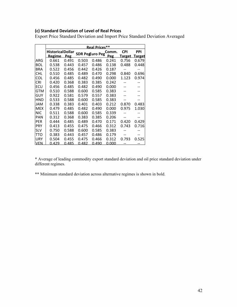
42

(c) Standard Deviation of Level of Real Prices Export Price Standard Deviation and Import Price Standard Deviation Averaged

* Average of leading commodity export standard deviation and oil price standard deviation under different regimes.  ** Minimum standard deviation across alternative regimes is shown in bold.

Historical Regime

Dollar Peg SDR PegEuro Peg

Comm. Peg

CPI Target

PPI Target

ARG 0.661 0.491 0.503 0.486 0.241 0.756 0.679BOL 0.538 0.443 0.457 0.486 0.138 0.488 0.448BRA 0.522 0.456 0.442 0.426 0.187  ‐‐  ‐‐CHL 0.510 0.485 0.489 0.470 0.298 0.840 0.696COL 0.456 0.485 0.482 0.490 0.000 1.123 0.974CRI 0.420 0.368 0.383 0.385 0.242 ‐‐ ‐‐ECU 0.456 0.485 0.482 0.490 0.000  ‐‐  ‐‐GTM 0.510 0.588 0.600 0.585 0.383 ‐‐ ‐‐GUY 0.922 0.581 0.579 0.557 0.383  ‐‐  ‐‐HND 0.533 0.588 0.600 0.585 0.383 ‐‐ ‐‐JAM 0.338 0.383 0.401 0.403 0.212 0.870 0.483MEX 0.479 0.485 0.482 0.490 0.000 0.975 1.030NIC 0.511 0.588 0.600 0.585 0.339  ‐‐  ‐‐PAN 0.312 0.368 0.383 0.385 0.206 ‐‐ ‐‐PER 0.444 0.485 0.489 0.470 0.171 0.420 0.429PRY 0.413 0.455 0.475 0.466 0.312 0.743 0.716SLV 0.750 0.588 0.600 0.585 0.383  ‐‐  ‐‐TTO 0.383 0.443 0.457 0.486 0.179 ‐‐ ‐‐URY 0.504 0.455 0.475 0.466 0.312 0.793 0.525VEN 0.429 0.485 0.482 0.490 0.000 ‐‐ ‐‐

Real Prices**

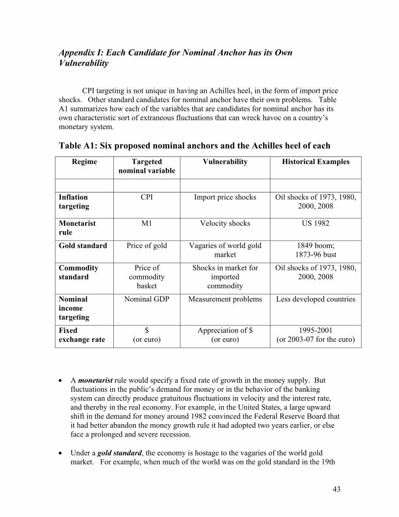
43

Appendix I: Each Candidate for Nominal Anchor has its Own Vulnerability

CPI targeting is not unique in having an Achilles heel, in the form of import price

shocks. Other standard candidates for nominal anchor have their own problems. Table A1 summarizes how each of the variables that are candidates for nominal anchor has its own characteristic sort of extraneous fluctuations that can wreck havoc on a country’s monetary system. Table A1: Six proposed nominal anchors and the Achilles heel of each

Regime Targeted nominal variable

Vulnerability Historical Examples

Inflation targeting

CPI

Import price shocks Oil shocks of 1973, 1980, 2000, 2008

Monetarist rule

M1 Velocity shocks US 1982

Gold standard Price of gold Vagaries of world gold market

1849 boom; 1873-96 bust

Commodity standard

Price of commodity

basket

Shocks in market for imported

commodity

Oil shocks of 1973, 1980, 2000, 2008

Nominal income targeting

Nominal GDP Measurement problems Less developed countries

Fixed exchange rate

$ (or euro)

Appreciation of $ (or euro)

1995-2001 (or 2003-07 for the euro)

A monetarist rule would specify a fixed rate of growth in the money supply. But

fluctuations in the public’s demand for money or in the behavior of the banking system can directly produce gratuitous fluctuations in velocity and the interest rate, and thereby in the real economy. For example, in the United States, a large upward shift in the demand for money around 1982 convinced the Federal Reserve Board that it had better abandon the money growth rule it had adopted two years earlier, or else face a prolonged and severe recession.

Under a gold standard, the economy is hostage to the vagaries of the world gold

market. For example, when much of the world was on the gold standard in the 19th

44

century, global monetary conditions depended on the output of the world’s gold mines. The California gold rush from 1849 was associated with a mid-century increase in liquidity and a resulting increase in the global price level. The absence of major discoveries of gold between 1873 and 1896 helps explain why price levels fell dramatically over this period. In the late 1890s, the gold rushes in Alaska and South Africa were each again followed by new upswings in the price level. Thus the system did not in fact guarantee stability.52

One proposal is that monetary policy should target a basket of basic mineral and

agricultural commodities. The idea is that a broad-based commodity standard of this sort would not be subject to the vicissitudes of a single commodity such as gold, because fluctuations of its components would average out somewhat.53 The proposal might work if the basket reflected the commodities produced and exported by the country in question. But for a country that is a net importer of oil, wheat, and other mineral and agricultural commodities, such a peg gives precisely the wrong answer in a year when the prices of these import commodities go up. Just when the domestic currency should be depreciating to accommodate an adverse movement in the terms of trade, it appreciates instead. Chile should not peg to oil, and Trinidad should not peg to wheat.

The need for robustness with respect to import price shocks argues for the superiority

of nominal income targeting over inflation targeting.54 A practical argument against nominal income targeting is the difficulty of timely measurement. For developing countries in particular, the data are sometimes available only with a delay of one or two years.

Under a fixed exchange rate, fluctuations in the value of the particular currency to

which the home country is pegged can produce needless volatility in the country’s international price competitiveness. For example, the appreciation of the dollar from 1995 and 2001 was also an appreciation for whatever currencies were linked to the dollar. Regardless the extent to which one considers the late-1990s dollar appreciation to have been based in the fundamentals of the US economy, there was no necessary connection to the fundamentals of smaller dollar-linked economies. The problem was particularly severe for some far-flung economies that had adopted currency boards over the preceding decade: Hong Kong, Argentina, and Lithuania.

Dollar-induced overvaluation was also one of the problems facing such victims of currency crisis as Mexico (1994), Thailand and Korea (1997), Russia (1998), Brazil (1999) and Turkey (2001), even though none of these countries had formal rigid links to the dollar. It is enough for the dollar to exert a large pull on the country’s currency to

52 Cooper (1985), Eichengrenn (1985) or Hall (1982). 54 Velocity shocks argue for the superiority of nominal income targeting over a monetarist rule. Frankel (1995) demonstrates the point mathematically, using the framework of Rogoff (1985), and gives other references on nominal income targeting.

45

create strains. The loss of competitiveness in non-dollar export markets adversely impacts such measures of economic health as real overvaluation, exports, the trade balance, and growth, or such measures of financial health as the ratios of current account to GDP, debt to GDP, debt service to exports, or reserves to imports.

This brings us back to the current fashion of targeting the inflation rate or CPI. To

some, PEP may sound similar to inflation targeting. But, as already noted, a key difference between the CPI and the export price is the terms of trade. When there is an adverse movement in the terms of trade, one would like the currency to depreciate, while price level targeting can have the opposite implication. If the central bank has been constrained to hit an inflation target, oil price shocks (as in 1973, 1979, 2000, or 2008), for example, will require an oil-importing country to tighten monetary policy. The result can be sharp falls in national output. Thus under rigid inflation targeting, supply or terms-of-trade shocks can produce unnecessary and excessive fluctuations in the level of economic activity.

46

Appendix 2: Stabilizing Properties of Pegging the Export Price vs. Exchange Rate and CPI Rules

The theoretical model is a two-sector version of Frankel,"Monetary Regime Choices for a Semi-Open Country," in Capital Controls, Exchange Rates and Monetary Policy in the World Economy, edited by Sebastian Edwards, Cambridge University Press, 1995: 35-69; which followed closely in the path of Kenneth Rogoff, "The Optimal Degree of Commitment to an Intermediate Monetary Target." Quarterly Journal of Economics 100, November, 1985; which in turn introduced shocks into the Barro-Gordon model dynamically-consistent monetary policy.

Assumptions

A supply relationship in each of two production sectors:

nennnn uppbyy )( (1)

xe

xxxx uppdyy )( (2)

where yn & yx output of nontraded & export sectors, respectively;

ny & xy potential output in the two sectors;

pn & px prices in two sectors (in domestic currency) pn

e & pxe expected prices;

un & ux supply disturbances; all in logs.

The country is a price-taker on world markets for exports and imports: px = s + εx , (3) pim = s + εim , (4)

where s exchange rate, spot price domestic currency / $, εx fluctuating $ price of export commodity; εim fluctuating $ price of import good.

Price indices (CPI & GDP deflator) include the nontraded good and the international good, with weights f and (1-f), respectively:

cpi = (f)pim +(1-f)pn , (5) p = (f)px + (1-f) pn . (6)

Money market equilibrium: m = p + y - v, (9)

and exchange rate equation s = m - y + e. (10)

47

where m money supply, y an index of total output, v velocity shocks e shocks in exchange rate equation. Objective is to minimize quadratic loss function:

L = a (cpi) 2 + f(yx-yx’) 2 + (1-f)(yn-yn’)

2 , (7) Results (The derivations are omitted, to save space.)

Table A2a Objective: Stabilize export revenue

Coefficient on:

εim

2

εx2

(v-e)2

ux

2

un2

Exchange rate peg

Equation (17)

0

(1+d)2

0

1

0

CPI rule (29) f 2 + (1+d)f 2

f 2 + (1+d)f2 + (1+d)

1+(1+d) 2 1 0

PEP (24) 0 1 0 1 0

=> PEP always dominates, so long as d > 0 and εx2 > 0.

Table

A2b

Objective: Stabilize CPI and output in the NTG and X sectors

Coefficient on:

εim2

εx

2

(v-e)2

ux2

un2

Exchange rate peg

(19) a f2 af2+ fd2 +

f 2b2

f1

1 a + b2

f1

1

f 1-f

CPI rule (32) b2f3 (1-f)

d2f3 + fd2 + b2(f3/1-f))]

fd 2 + b2(f2/1-f))

f 1-f

PEP

(25) a f 2 a f 2 a[(1-f)/f] 2

+ b2/(1-f)

f 1-f

48

=> PEP vs. Exchange rate peg:

Even if there are no export price shocks, then the expected loss is smaller under the PEP rule if f > 1/2, i.e., if the foreign sector is larger than the domestic sector.

To the extent that export price shocks are greater than 0, the case is stronger, because εx shocks affect output of both exports and nontraded goods, whereas PEP insulates the real economy against them. If εx shocks are large, then PEP dominates regardless of parameter values. PEP vs. CPI rule:

If a is large, i.e., if stabilizing CPI is top priority, then terms of trade and exchange rate shocks hurt more under the PEP rule than under inflation targeting. But shocks to world prices destabilize both output terms under the CPI rule, while PEP insulates the real economy; thus if a is small (relative to b & d), PEP dominates.

49

Appendix 3: Data Sources and Computation Methods Data Sources Variable Source

Commodity Prices International Financial Statistics (IFS) and Global Financial Statistics (GFS)

Composition of commodity exports World Bank analysis

Exports IFS

Imports IFS

Export Price Index IFS

Consumer Price Index (CPI) IFS

Producer Price Index (PPI) IFS, Countries' National Statistical Institute and Central Bank

Wholesale Price Index (WPI) IFS, Countries' National Statistical Institute and Central Bank

Exchange Rates IFS

CPI detailed decomposition Countries' National Statistical Institute

PPI detailed decomposition Countries' National Statistical Institute

Non Tradables CPI Countries' Central Bank

Tradables CPI Countries' Central Bank Computation Methods

1. Simulation of Export Prices

A profit-maximizing firm that is competitive in its product and input markets will produce in relation to the ratio of the price of the export good to the price of its variable inputs. If its production is for simplicity taken to be Cobb-Douglas, with labor the only variable factor of production, then in logs we have )( wpxLogX x

where px is the log of the domestic currency price of the export good in question, w is the log of the wage in local currency, and the supply elasticity depends on labor’s share.

$$lcxx spp

Where p$x is the log dollar price of the export good on world markets, which fluctuates

exogenously; and s$

lc is the log dollar value of the local currency, which depends both on the country’s exchange rate policy and fluctuations in the dollar’s value. A country can get into trouble under a regime where s$

lc is fixed, because a decline in p$x hurts exports in proportion . (In dollar terms, which may be the most relevant measure if a country has incurred debts in dollars, the loss of export revenue is (1+ ) times the fall in p$

x.) But the country can also get into trouble if the exchange rate s$

lc floats, and thereby introduces its own extraneous fluctuations into the equation. Assume that w is stable, a prospect that is more likely if expected inflation has been secured by means of one or another nominal anchor for monetary policy. Then to determine exports, whether in real terms or dollar terms, we want to focus on: $$

lcxx spp

50

The way to do that is to set the dollar price of the domestic currency equal to the dollar price of the export commodity: $$

lcx sp

Operationally, this is the way to implement a commitment to peg the domestic price of the export commodity. Intuitively, by removing fluctuations in px, we may stabilize exports. (In the simulations, we focus on how various regimes would affect px-w, where we represent the domestic cost of variable inputs, w, by the domestic CPI). To repeat from above, the key variable is px-w, the price of exports relative to the cost of variable inputs, which could be defined as the real exchange rate. The path under the seven possible regimes is calculated as follows: Under actual history, $

$ xlc

x PSP and w = CPIlc .

Under a hypothetical dollar peg, 1$ lcS , so $xx PP and w = CPIUS.

Under a hypothetical DM or euro peg 55, DMlc SS $$ , so $$ xDM

x PSP and w = CPIG.

Under a hypothetical SDR, SDRlc SS $$ , so $$ xSDR

x PSP and w = CPISDR.56

Under a hypothetical commodity peg, xlc PS $$ , so 1xP and w = 1.

Under a hypothetical CPI target57, )/()100( $$$$ otgotgpmpmcxcxntgntglc PwPwPwPwS ,

$$ xlc

x PSP .

Under a hypothetical PPI target58, )/()100( $$$$ otgotgpmpmcxcxntgntglc PvPvPvPvS ,

$$ xlc

x PSP .

Under the CPI and PPI target, we have approximated non tradable goods’ prices using a 10-year moving average of the US CPI (assuming the target was implemented credibly since the start of the period under analysis). We use the CPI to measure the price of variable inputs, w. When the currency is hypothetically taken to be rigidly pegged to the dollar, SDR, or DM, then CPIHome is taken to be the CPI of the US, SDR, or Germany, respectively, under the assumption that the peg is strong enough and permanent enough to achieve convergence of inflation rates59. The path of the real price of commodities under the seven possible regimes is calculated as follows:

Under actual history, lcxlc

x CPIPSRP /$$

55 The exchange rate of the German Mark after 1999 is calculated as follows. S(DM/$) in 1999 = S(Euro/$) in 1999 * S(DM/Euro) in 1999; S(DM/$) in 2000 = S(DM/$) in 1999 * (1 + % change of the euro exchange rate). 56 The CPI for the SDR peg is constructed as a weighted average of USA CPI, UK CPI, France CPI and Germany CPI. To calculate this average we use the weight of each country’s currency in the SDR. 57 Rewrite the CPI equation from part 2. of this appendix as: CPI = wntg Pntg +wcx S Pcx$ + wpm S Ppm$ + wotg S Potg$ and solve for the exchange rate that maintains CPI constant. 58 Rewrite the PPI equation from part 2. of this appendix as: PPI = vntg Pntg +vcx S Pcx$ + vpm S Ppm$ + votg S Potg$ and solve for the exchange rate that maintains PPI constant. 59 When calculating the real exchange rate for the euro, we continue to use the German CPI.

51

Under a hypothetical dollar peg, ))(/( $$ KCPIPRP USxx

Under a hypothetical SDR peg, ))(/( $$ SDRSDRxSDR

x KCPIPSRP

Under a hypothetical DM or euro peg, ))(/( $$ DMGxDM

x KCPIPSRP

Under a hypothetical commodity peg, xx KRP

Under a hypothetical CPI target, ))(( $$ CPIxlc

x KPSRP

Under a hypothetical PPI target, ))(( $$ PPIxlc

x KPSRP

Where K$ , KSDR , KDM , Kx , KCPI and KPPI are constants calculated so as to make the log of the real price of the commodity on average over the 30 year period equal under each of the regimes to what it was in actual history.

We simulated import prices for LAC countries using this same methodology; instead of using the price of the leading commodity export in dollars we used the most important import prices in dollar terms as can be seen in tables 5a.

2. Simulation of CPI and PPI

To simulate the Consumer Price Index (CPI) and Producer Price Index (PPI) under different regimes we impose the following equations.

otgotgpmpmcxwcxntgntg

otgotgpmpmcxwcxntgntg

PvPvPvPvPPI

PwPwPwPwCPI

where: Pntg ≡ Price of non-traded goods in local terms. We assume that, at a horizon of less than 1 year, these prices would not be affected by differences in the exchange rate. Under the hypothetical counterfactual where a country would have been on a dollar peg all along, then its non tradable prices are given by the US CPI, since we assume that convergence would have taken place in the long run. Pcx ≡ Price of exports of leading mineral/agricultural commodity in local terms (we ignore trade barriers and define these tradable goods prices to equal the actual historically observed world dollar prices, times the exchange rate, which will differ depending on the regime assumed. Pox ≡ Price of other exports, which we approximate using Ppm ≡ Price of petroleum product imports. This is determined again as actual world dollar price times the simulated exchange rate. Potg ≡ Price of other tradable goods (i.e., excluding oil and the other commodities that are measured explicitly). Assume equal to world prices of the tradable goods times the exchange rate. wntg ≡ weight on ntg in CPI wcx ≡ weight on cx in CPI wpm ≡ weight on pm in CPI wotg ≡ weight on otg in CPI vntg ≡ weight on ntg in PPI vcx ≡ weight on cx in PPI vpm ≡ weight on pm in PPI votg ≡ weight on otg in PPI . We impose wntg ≡ vntg

52

To estimate the above mentioned weights, we followed these steps:

a. Obtain countries’ Non Tradable CPI and Tradable CPI series. b. Regress CPI against Non Tradable CPI to get wntg = vntg. c. Obtain detailed decomposition of CPI and PPI, and calculate weight of leading

commodity export (wcx and vcx) and weight of oil in CPI and PPI (wpm and vpm). d. Calculate weight of other tradable goods as the complement (i.e., 1 - wcx - wntg - wpm).

53

Appendix 4: Nominal and Real Log Export Prices, Simulated under alternative regimes Argentina

‐8

‐6

‐4

‐2

0

2

1970

1972

1974

1976

1978

1980

1982

1984

1986

1988

1990

1992

1994

1996

1998

2000

2002

2004

2006

2008

Argentina, Nominal Soybean Price(in natural log, mean substracted)

Historic regime

Dollar Peg

SDR Peg

Euro Peg

CPI Target

PPI Target

‐4.5

‐3.5

‐2.5

‐1.5

‐0.5

0.5

1.5

2.5

1970

1972

1974

1976

1978

1980

1982

1984

1986

1988

1990

1992

1994

1996

1998

2000

2002

2004

2006

2008

Argentina, Real Soybean Price(in natural log, mean substracted)

Historic regimeDollar Peg

SDR Peg

Euro Peg

Comm Peg

CPI Target

PPI Target

‐8

‐6

‐4

‐2

0

2

4

1970

1972

1974

1976

1978

1980

1982

1984

1986

1988

1990

1992

1994

1996

1998

2000

2002

2004

2006

2008

Argentina, Nominal Comm. Basket Price(in natural log, mean substracted)

Historic regime

Dollar Peg

SDR Peg

Euro Peg

‐1.5

‐1

‐0.5

0

0.5

1

1.5

1970

1972

1974

1976

1978

1980

1982

1984

1986

1988

1990

1992

1994

1996

1998

2000

2002

2004

2006

2008

Argentina, Real Comm. Basket Price(in natural log, mean substracted)

Historic regime

Dollar Peg

SDR Peg

Euro Peg

* Basket: Maize, soybeans, oil and wheat. Bolivia

‐10

‐8

‐6

‐4

‐2

0

2

4

1970

1972

1974

1976

1978

1980

1982

1984

1986

1988

1990

1992

1994

1996

1998

2000

2002

2004

2006

2008

Bolivia, Nominal Natural Gas Price(in natural log, mean substracted)

Historic regimeDollar Peg

SDR Peg

Euro Peg

CPI Target

PPI Target‐1.5

‐1

‐0.5

0

0.5

1

1.5

2

2.5

1970

1972

1974

1976

1978

1980

1982

1984

1986

1988

1990

1992

1994

1996

1998

2000

2002

2004

2006

2008

Bolivia, Real Natural Gas Price(in natural log, mean substracted)

Historic regimeDollar Peg

SDR Peg

Euro Peg

Comm Peg

CPI Target

PPI Target

54

‐10

‐8

‐6

‐4

‐2

0

2

4

1970

1972

1974

1976

1978

1980

1982

1984

1986

1988

1990

1992

1994

1996

1998

2000

2002

2004

2006

2008

Bolivia, Nominal Export Price (in natural log, mean substracted)

Historic regime

Dollar Peg

SDR Peg

Euro Peg

‐1.5

‐1

‐0.5

0

0.5

1

1.5

1970

1972

1974

1976

1978

1980

1982

1984

1986

1988

1990

1992

1994

1996

1998

2000

2002

2004

2006

2008

Bolivia, Real Export Price (in natural log, mean substracted)

Historic regime

Dollar Peg

SDR Peg

Euro Peg

Brazil

‐10

‐8

‐6

‐4

‐2

0

2

4

1970

1972

1974

1976

1978

1980

1982

1984

1986

1988

1990

1992

1994

1996

1998

2000

2002

2004

2006

2008

Brazil, Nominal Steel Price(in natural log, mean substracted)

Historic regime

Dollar Peg

SDR Peg

Euro Peg

‐1

‐0.5

0

0.5

1

1.5

1970

1972

1974

1976

1978

1980

1982

1984

1986

1988

1990

1992

1994

1996

1998

2000

2002

2004

2006

2008

Brazil, Real Steel Price(in natural log, mean substracted)

Historic regime

Dollar Peg

SDR Peg

Euro Peg

‐8

‐6

‐4

‐2

0

2

4

1970

1972

1974

1976

1978

1980

1982

1984

1986

1988

1990

1992

1994

1996

1998

2000

2002

2004

2006

2008

Brazil,  Iron ore Nominal Price(in natural log, mean substracted)

Historic regime

Dollar Peg

SDR Peg

Euro Peg

‐1.5

‐1

‐0.5

0

0.5

1

1.5

1970

1972

1974

1976

1978

1980

1982

1984

1986

1988

1990

1992

1994

1996

1998

2000

2002

2004

2006

2008

Brazil, Iron Ore Real Price(in natural log, mean substracted)

Historic regime

Dollar Peg

SDR Peg

Euro Peg

‐8

‐6

‐4

‐2

0

2

4

1970

1972

1974

1976

1978

1980

1982

1984

1986

1988

1990

1992

1994

1996

1998

2000

2002

2004

2006

2008

Brazil, Nominal Comm. Basket Price(in natural log, mean substracted)

Historic regime

Dollar Peg

SDR Peg

Euro Peg

‐0.8

‐0.6

‐0.4

‐0.2

0

0.2

0.4

0.6

0.8

1

1970

1972

1974

1976

1978

1980

1982

1984

1986

1988

1990

1992

1994

1996

1998

2000

2002

2004

2006

2008

Brazil, Real Comm. Basket Price(in natural log, mean substracted)

Historic regime

Dollar Peg

SDR Peg

Euro Peg

* Basket: Iron Ore, Steel scrap, oil and sugar.

55

‐10

‐8

‐6

‐4

‐2

0

2

41970

1972

1974

1976

1978

1980

1982

1984

1986

1988

1990

1992

1994

1996

1998

2000

2002

2004

2006

2008

Brazil, Nominal Export Price(in natural log, mean substracted)

Historic regime

Dollar Peg

SDR Peg

Euro Peg

‐1.5

‐1

‐0.5

0

0.5

1

1.5

1970

1972

1974

1976

1978

1980

1982

1984

1986

1988

1990

1992

1994

1996

1998

2000

2002

2004

2006

2008

Brazil, Real Export Price(in natural log, mean substracted)

Historic regime

Dollar Peg

SDR Peg

Euro Peg

Chile

‐10

‐8

‐6

‐4

‐2

0

2

4

1970

1972

1974

1976

1978

1980

1982

1984

1986

1988

1990

1992

1994

1996

1998

2000

2002

2004

2006

2008

Chile, Nominal Copper Price(in natural log, mean substracted)

Historic regime

Dollar Peg

SDR Peg

Euro Peg

CPI Target

PPI Target

‐5.5

‐3.5

‐1.5

0.5

2.5

4.5

6.5

8.5

10.5

1970

1972

1974

1976

1978

1980

1982

1984

1986

1988

1990

1992

1994

1996

1998

2000

2002

2004

2006

2008

Chile, Real Copper Price(in log, mean substracted)

Historic regime

Dollar Peg

SDR Peg

Euro Peg

Comm Peg

CPI Target

PPI Target

Colombia

‐5

‐4

‐3

‐2

‐1

0

1

2

3

4

1970

1972

1974

1976

1978

1980

1982

1984

1986

1988

1990

1992

1994

1996

1998

2000

2002

2004

2006

2008

Colombia, Nominal Oil Price(in natural log, mean substracted)

Historic regime

Dollar Peg

SDR Peg

Euro Peg

CPI Target

PPI Target

‐5.00

‐4.00

‐3.00

‐2.00

‐1.00

0.00

1.00

2.00

3.00

4.00

5.00

1970

1972

1974

1976

1978

1980

1982

1984

1986

1988

1990

1992

1994

1996

1998

2000

2002

2004

2006

2008

Colombia, Real Oil Price(in natural log, mean substracted)

Historic regimeDollar PegSDR Peg

Euro Peg

Comm PegCPI TargetPPI Target

56

‐4

‐3

‐2

‐1

0

1

2

31970

1972

1974

1976

1978

1980

1982

1984

1986

1988

1990

1992

1994

1996

1998

2000

2002

2004

2006

2008

Colombia,  Nominal Coffee Price(in natural log, mean substracted)

Historic regime

Dollar Peg

SDR Peg

Euro Peg

‐2.00

‐1.50

‐1.00

‐0.50

0.00

0.50

1.00

1.50

2.00

1970

1972

1974

1976

1978

1980

1982

1984

1986

1988

1990

1992

1994

1996

1998

2000

2002

2004

2006

2008

Colombia, Real Coffee Price(in natural log, mean substracted)

Historic regime

Dollar Peg

SDR Peg

Euro Peg

‐1.2‐1

‐0.8‐0.6‐0.4‐0.2

00.20.40.60.8

1970

1972

1974

1976

1978

1980

1982

1984

1986

1988

1990

1992

1994

1996

1998

2000

2002

2004

2006

2008

Colombia, Nominal Export Price(in natural log, mean substracted)

Historic regime

Dollar Peg

SDR Peg

Euro Peg

‐0.30

‐0.20

‐0.10

0.00

0.10

0.20

0.30

0.40

1970

1972

1974

1976

1978

1980

1982

1984

1986

1988

1990

1992

1994

1996

1998

2000

2002

2004

2006

2008

Colombia, Real Export Price(in natural log, mean substracted)

Historic regime

Dollar Peg

SDR Peg

Euro Peg

Costa Rica

‐4

‐3

‐2

‐1

0

1

2

3

4

1970

1972

1974

1976

1978

1980

1982

1984

1986

1988

1990

1992

1994

1996

1998

2000

2002

2004

2006

2008

Costa rica, Nominal Bananas Price(in log, mean substracted)

Historic regime

Dollar Peg

SDR Peg

Euro Peg

‐1.50

‐1.00

‐0.50

0.00

0.50

1.00

1.50

1970

1972

1974

1976

1978

1980

1982

1984

1986

1988

1990

1992

1994

1996

1998

2000

2002

2004

2006

2008

Costa Rica, Real Bananas Price(in natural log, mean substracted)

Historic regime

Dollar Peg

SDR Peg

Euro Peg

57

‐4

‐3

‐2

‐1

0

1

2

31970

1972

1974

1976

1978

1980

1982

1984

1986

1988

1990

1992

1994

1996

1998

2000

2002

2004

2006

2008

Costa rica, Nominal Coffee Price(in log, mean substracted)

Historic regimeDollar Peg

SDR Peg

Euro Peg

‐2.00

‐1.50

‐1.00

‐0.50

0.00

0.50

1.00

1.50

2.00

1970

1972

1974

1976

1978

1980

1982

1984

1986

1988

1990

1992

1994

1996

1998

2000

2002

2004

2006

2008

Costa Rica, Real Coffee Price(in log, mean substracted)

Historic regime

Dollar Peg

SDR Peg

Euro Peg

Ecuador

‐6

‐4

‐2

0

2

4

6

1970

1972

1974

1976

1978

1980

1982

1984

1986

1988

1990

1992

1994

1996

1998

2000

2002

2004

2006

2008

Ecuador, Nominal Oil Price(in natural log, mean substracted)

Historic regime

Dollar Peg

SDR Peg

Euro Peg‐1.50

‐1.00

‐0.50

0.00

0.50

1.00

1.50

1970

1972

1974

1976

1978

1980

1982

1984

1986

1988

1990

1992

1994

1996

1998

2000

2002

2004

2006

2008

Ecuador, Real Oil Price(in natural log, mean substracted)

Historic regime

Dollar Peg

SDR Peg

Euro Peg

‐6

‐4

‐2

0

2

4

6

1970

1972

1974

1976

1978

1980

1982

1984

1986

1988

1990

1992

1994

1996

1998

2000

2002

2004

2006

2008

Ecuador, Nominal Export Price(in log, mean substracted)

Historic regime

Dollar Peg

SDR Peg

Euro Peg ‐1.00

‐0.50

0.00

0.50

1.00

1970

1972

1974

1976

1978

1980

1982

1984

1986

1988

1990

1992

1994

1996

1998

2000

2002

2004

2006

2008

Ecuador, Real Export Price(in natural log, mean substracted)

Historic regime

Dollar Peg

SDR Peg

Euro Peg

58

El Salvador

‐2

‐1.5

‐1

‐0.5

0

0.5

1

1.5

1970

1972

1974

1976

1978

1980

1982

1984

1986

1988

1990

1992

1994

1996

1998

2000

2002

2004

2006

2008

El Salvador, Nominal Coffee Price(in natural log, mean substracted) 

Historic regime

Dollar Peg

SDR Peg

Euro Peg‐2.00‐1.50‐1.00‐0.500.000.501.001.502.002.50

1970

1972

1974

1976

1978

1980

1982

1984

1986

1988

1990

1992

1994

1996

1998

2000

2002

2004

2006

2008

El Salvador, Real Coffee Price(in natural log, mean substracted)

Historic regime

Dollar Peg

SDR Peg

Euro Peg

Guatemala

‐2

‐1.5

‐1

‐0.5

0

0.5

1

1.5

2

1970

1972

1974

1976

1978

1980

1982

1984

1986

1988

1990

1992

1994

1996

1998

2000

2002

2004

2006

2008

Guatemala, Nominal Coffee Price(in natural log, mean substracted)

Historic regime

Dollar Peg

SDR Peg

Euro Peg

‐2.00

‐1.50

‐1.00

‐0.50

0.00

0.50

1.00

1.50

2.00

1970

1972

1974

1976

1978

1980

1982

1984

1986

1988

1990

1992

1994

1996

1998

2000

2002

2004

2006

2008

Guatemala, Real Coffee Price(in natural log, mean substracted)

Historic regime

Dollar Peg

SDR Peg

Euro Peg

Guyana

‐4

‐3

‐2

‐1

0

1

2

3

1970

1972

1974

1976

1978

1980

1982

1984

1986

1988

1990

1992

1994

1996

1998

2000

2002

2004

2006

2008

Guyana, Nominal Sugar Price(in natural log, mean substracted)

Historic regime

Dollar Peg

SDR Peg

Euro Peg

‐2.50

‐2.00

‐1.50

‐1.00

‐0.50

0.00

0.50

1.00

1.50

2.00

2.50

1970

1972

1974

1976

1978

1980

1982

1984

1986

1988

1990

1992

1994

1996

1998

2000

2002

2004

2006

2008

Guyana, Real Sugar Price(in natural log, mean substracted)

Historic regime

Dollar Peg

SDR Peg

Euro Peg

59

Honduras

‐2

‐1.5

‐1

‐0.5

0

0.5

1

1.5

2

1970

1972

1974

1976

1978

1980

1982

1984

1986

1988

1990

1992

1994

1996

1998

2000

2002

2004

2006

2008

Honduras, Nominal Coffee Price(in natural log, mean substracted)

Historic regime

Dollar Peg

SDR Peg

Euro Peg‐2.00

‐1.50

‐1.00

‐0.50

0.00

0.50

1.00

1.50

2.00

1970

1972

1974

1976

1978

1980

1982

1984

1986

1988

1990

1992

1994

1996

1998

2000

2002

2004

2006

2008

Honduras, Real Coffee Price(in natural log, mean substracted)

Historic regime

Dollar Peg

SDR Peg

Euro Peg

Jamaica

‐4

‐3

‐2

‐1

0

1

2

3

4

1970

1972

1974

1976

1978

1980

1982

1984

1986

1988

1990

1992

1994

1996

1998

2000

2002

2004

2006

2008

Jamaica, Nominal Aluminium Price(in natural log, mean substracted)

Historic regime

Dollar Peg

SDR Peg

Euro Peg

CPI Target

PPI Target ‐4.50

‐2.50

‐0.50

1.50

3.50

5.50

1970

1972

1974

1976

1978

1980

1982

1984

1986

1988

1990

1992

1994

1996

1998

2000

2002

2004

2006

2008

Jamaica, Real Aluminium Price(in natural log, mean substracted)

Historic regime

Dollar Peg

SDR Peg

Euro Peg

Comm Peg

CPI Target

PPI Target

Mexico

‐8

‐6

‐4

‐2

0

2

4

6

1970

1972

1974

1976

1978

1980

1982

1984

1986

1988

1990

1992

1994

1996

1998

2000

2002

2004

2006

2008

Mexico, Nominal Oil Price(in natural log, mean substracted) 

Historic regime

Dollar Peg

SDR Peg

Euro Peg

CPI Target

PPI Target

‐2.00

‐1.50

‐1.00

‐0.50

0.00

0.50

1.00

1.50

2.00

1970

1972

1974

1976

1978

1980

1982

1984

1986

1988

1990

1992

1994

1996

1998

2000

2002

2004

2006

2008

Mexico, Real Oil Price(in natural log, mean substracted)

Historic regime

Dollar Peg

SDR Peg

Euro Peg

Comm Peg

CPI Target

PPI Target

60

Nicaragua

‐8

‐6

‐4

‐2

0

2

4

1970

1972

1974

1976

1978

1980

1982

1984

1986

1988

1990

1992

1994

1996

1998

2000

2002

2004

2006

2008

Nicaragua, Nominal Coffee Price(in natural log, mean substracted) 

Historic regime

Dollar Peg

SDR Peg

Euro Peg

‐2.00

‐1.50

‐1.00

‐0.50

0.00

0.50

1.00

1.50

2.00

1970

1972

1974

1976

1978

1980

1982

1984

1986

1988

1990

1992

1994

1996

1998

2000

2002

2004

2006

2008

Nicaragua, Real Coffee Price(in natural log, mean substracted)

Historic regime

Dollar Peg

SDR Peg

Euro Peg

Panama

‐1.5

‐1

‐0.5

0

0.5

1

1.5

1970

1972

1974

1976

1978

1980

1982

1984

1986

1988

1990

1992

1994

1996

1998

2000

2002

2004

2006

2008

Panama, Nominal Bananas Price(in natural log, mean substracted)

Historic regime

Dollar Peg

SDR Peg

Euro Peg

‐0.80

‐0.60

‐0.40

‐0.20

0.00

0.20

0.40

0.601970

1972

1974

1976

1978

1980

1982

1984

1986

1988

1990

1992

1994

1996

1998

2000

2002

2004

2006

2008

Panama, Real Bananas Price(in natural log, mean substracted)

Historic regime

Dollar Peg

SDR Peg

Euro Peg

Peru

‐8‐7‐6‐5‐4‐3‐2‐10123

1970

1972

1974

1976

1978

1980

1982

1984

1986

1988

1990

1992

1994

1996

1998

2000

2002

2004

2006

2008

Peru, Nominal Copper Price(in natural log, mean substracted)

Historic regime

Dollar Peg

SDR Peg

Euro Peg

CPI Target

PPI Target ‐1.50

‐0.50

0.50

1.50

2.50

3.50

4.50

1970

1972

1974

1976

1978

1980

1982

1984

1986

1988

1990

1992

1994

1996

1998

2000

2002

2004

2006

2008

Peru, Real Copper Price(in natural log, mean substracted)

Historic regime

Dollar Peg

SDR Peg

Euro Peg

Comm Peg

CPI Target

PPI Target

61

‐8‐7‐6‐5‐4‐3‐2‐1012

1970

1972

1974

1976

1978

1980

1982

1984

1986

1988

1990

1992

1994

1996

1998

2000

2002

2004

2006

2008

Peru, Nominal Gold Price(in natural log, mean substracted)

Historic regime

Dollar Peg

SDR Peg

Euro Peg

‐1.50

‐1.00

‐0.50

0.00

0.50

1.00

1.50

1970

1972

1974

1976

1978

1980

1982

1984

1986

1988

1990

1992

1994

1996

1998

2000

2002

2004

2006

2008

Peru, Real Gold Price(in natural log, mean substracted) 

Historic regime

Dollar Peg

SDR Peg

Euro Peg

‐8

‐6

‐4

‐2

0

2

4

1970

1972

1974

1976

1978

1980

1982

1984

1986

1988

1990

1992

1994

1996

1998

2000

2002

2004

2006

2008

Peru, Nominal Export Price(in natural log, mean substracted)

Historic regime

Dollar Peg

SDR Peg

Euro Peg

‐1.50

‐1.00

‐0.50

0.00

0.50

1.00

1.50

1970

1972

1974

1976

1978

1980

1982

1984

1986

1988

1990

1992

1994

1996

1998

2000

2002

2004

2006

2008

Peru, Real Export Price(in natural log, mean substracted)

Historic regime

Dollar Peg

SDR Peg

Euro Peg

Paraguay

‐3

‐2

‐1

0

1

2

3

1970

1972

1974

1976

1978

1980

1982

1984

1986

1988

1990

1992

1994

1996

1998

2000

2002

2004

2006

2008

Paraguay,  Beef Nominal Price(in natural log, mean substracted)

Historic regimeDollar Peg

SDR Peg

Euro Peg

CPI Target

PPI Target‐4.00

‐3.00

‐2.00

‐1.00

0.00

1.00

2.00

3.00

4.00

1970

1972

1974

1976

1978

1980

1982

1984

1986

1988

1990

1992

1994

1996

1998

2000

2002

2004

2006

2008

Paraguay, Real Beef Price(in natural log, mean substracted)

Historic regimeDollar Peg

SDR Peg

Euro Peg

Comm Peg

CPI Target

PPI Target

62

Trinidad and Tobago

‐2.5

‐2

‐1.5

‐1

‐0.5

0

0.5

1

1.5

2

1970

1972

1974

1976

1978

1980

1982

1984

1986

1988

1990

1992

1994

1996

1998

2000

2002

2004

2006

2008

Trinidad and Tobago, Nominal Natural Gas Price(in natural log, mean substracted)

Historic regime

Dollar Peg

SDR Peg

Euro Peg

‐1.00

‐0.80

‐0.60

‐0.40

‐0.20

0.00

0.20

0.40

0.60

0.80

1.00

1970

1972

1974

1976

1978

1980

1982

1984

1986

1988

1990

1992

1994

1996

1998

2000

2002

2004

2006

2008

Trinidad and Tobago, Real Natural Gas Price(in natural log, mean substracted)

Historic regime

Dollar Peg

SDR Peg

Euro Peg

Uruguay

‐8

‐6

‐4

‐2

0

2

4

6

1970

1972

1974

1976

1978

1980

1982

1984

1986

1988

1990

1992

1994

1996

1998

2000

2002

2004

2006

2008

Uruguay, Nominal Beef Price(in natural log, mean substracted)

Historic regime

Dollar Peg

SDR Peg

Euro Peg

CPI Target

PPI Target

‐9.50

‐7.50

‐5.50

‐3.50

‐1.50

0.50

2.50

4.50

6.50

8.501970

1972

1974

1976

1978

1980

1982

1984

1986

1988

1990

1992

1994

1996

1998

2000

2002

2004

2006

2008

Uruguay, Real Beef Price(in natural log, mean substracted)

Historic regime

Dollar Peg

SDR Peg

Euro Peg

Comm Peg

CPI Target

PPI Target

Venezuela

‐6

‐4

‐2

0

2

4

6

1970

1972

1974

1976

1978

1980

1982

1984

1986

1988

1990

1992

1994

1996

1998

2000

2002

2004

2006

2008

Venezuela, Nominal Oil Price(in natural log, mean substracted)

Historic regime

Dollar Peg

SDR Peg

Euro Peg

‐1.50

‐1.00

‐0.50

0.00

0.50

1.00

1.50

1970

1972

1974

1976

1978

1980

1982

1984

1986

1988

1990

1992

1994

1996

1998

2000

2002

2004

2006

2008

Venezuela, Real Oil Price(in natural log, mean substracted)

Historic regime

Dollar Peg

SDR Peg

Euro Peg