A Comparison of Threshold Cointegration andMarkov-Switching Vector Error Correction

Models in Price Transmission Analysisby

Rico Ihle and Stephan von Cramon-Taubadel

Suggested citation format:

Ihle, R., and S. v. Cramon-Taubadel. 2008. “A Comparison of Threshold Cointegration and Markov-Switching Vector Error Correction Models in Price Transmission Analysis.” Proceedings of the NCCC-134 Conference on Applied Commodity Price Analysis, Forecasting, and Market Risk Management. St. Louis, MO. [http://www.farmdoc.uiuc.edu/nccc134].

A Comparison of Threshold Cointegration and Markov-Switching Vector ErrorCorrection Models in Price Transmission Analysis

Rico Ihle

and

Stephan von Cramon-Taubadel∗

Paper presented at the NCCC-134 Conference on Applied Commodity Price Analysis,Forecasting, and Market Risk Management

St. Louis, Missouri, April 21-22, 2008

Copyright 2008 by Rico Ihle and Stephan von Cramon-Taubadel.All rights reserved. Readers may make verbatim copies of this document for non-commercial

purposes by any means, provided that this copyright notice appears on all such copies.

∗ Rico Ihle (rihle@gwdg.de) is a PhD student in the Centre for Statistics ZfS and the Department of AgriculturalEconomics and Rural Development at the Georg-August-Universität Göttingen, Germany; Stephan von Cramon-Taubadel is Professor in the Department of Agricultural Economics and Rural Development at the Georg-August-Universität Göttingen, Germany.

A Comparison of Threshold Cointegration and Markov-Switching Vector ErrorCorrection Models in Price Transmission Analysis

We compare two regime-dependent econometric models for price transmission analysis,namely the threshold vector error correction model and Markov-switching vector errorcorrection model. We first provide a detailed characterization of each of the models which isfollowed by a comprehensive comparison. We find that the assumptions regarding the natureof their regime-switching mechanisms are fundamentally different so that each model issuitable for a certain type of nonlinear price transmission. Furthermore, we conduct a MonteCarlo experiment in order to study the performance of the estimation techniques of bothmodels for simulated data. We find that both models are adequate for studying pricetransmission since their characteristics match the underlying economic theory and allowhence for an easy interpretation. Nevertheless, the results of the corresponding estimationtechniques do not reproduce the true parameters and are not robust against nuisanceparameters. The comparison is supplemented by a review of empirical studies in pricetransmission analysis in which mostly the threshold vector error correction model is applied.

Keywords: price transmission; market integration; threshold vector error correctionmodel; Markov-switching vector error correction model; comparison;nonlinear time series analysis

1 Introduction

Economists have devoted considerable attention to testing the Law of One Price (LOP) in avariety of settings, and agricultural economists in particular have generated an extensiveliterature on the empirical analysis of price transmission (PT) along spatial (prices for ahomogeneous commodity at different locations - e.g. wheat in France and Germany) andvertical (prices for a commodity at different stages of processing - e.g. wheat-flour-bread)dimensions. Early studies focused on correlations or linear time series analysis involvingprices, but in recent years attention has increasingly turned to the use of models that cancapture the regime-dependent nature of relationships between prices. In a spatial context, thekey insight, derived from Takayama and Judge (1971), is that prices will only co-move ifspatial arbitrage conditions are binding (Baulch, 1994). If the difference between prices attwo locations is greater than the cost of trade between these locations, then arbitrage willdrive the price difference net of transaction costs to zero, and this equilibrating mechanismwill lead to an observable relationship between the prices in question. If the differencebetween these prices is less than the transaction costs, however, arbitrage will not take placeand in the simplest case the prices will move independently of one another. The result is atwo-regime model of PT that extends to three regimes if the possibility of trade reversal isconsidered, and possibly more regimes if factors such as links to third markets orequilibrating mechanisms other than physical trade are accounted for.

The threshold vector error correction model has been used extensively in PT analysis(Goodwin and Piggott, 2001, etc.). Recently, Brümmer et al. (2008) propose the use of the

2

Markov-switching vector error correction model to study price transmission in a verticalcontext between wheat and flour in Ukraine. So far no systematic attempt has been made tocontrast and compare these models as regards their theoretical underpinnings and theirperformance and interpretation in the context of PT. In this paper we carry out such acomparison in order to provide some indication regarding the common and differing featuresof both models. Both models allow for regime-switching; does this characteristic imply thatthey may be used interchangeably and lead to congruent results? We show that this is not thecase and that each approach suits best particular analytical objectives in PT analysis. Thecomparison discusses the most important aspects for the empirical application of both modelsin PT analysis in detail in order to give some indication for the application of both models.

Section 2 outlines the relationship of both models to other time series models by introducingthe class of nonlinear time series models in general and the subclass of thresholdautoregressive models. These considerations are followed by a detailed characterization ofthe threshold and the Markov-switching vector error correction model, respectively, byfocusing on the basic idea, the model structure, the estimation and the interpretation of each.Section 3 provides a conceptual comparison of the characteristics of both models outlinedbefore. It is supplemented by a simulation study which assesses the performance of theestimation methods of each model. The last section summarizes and draws conclusions.Appendix A provides a literature review of applications of the threshold vector errorcorrection model to PT analysis. Appendix B contains details on the simulation study.

2 Model Review

2.1 Classification of nonlinear time series models

Many model classes for nonlinear time series analysis were developed during the second halfof the seventies and the eighties of the past century.1 Tong (1978) introduced the class ofso-called threshold models. Fairly general formulations of nonlinear models have beendeveloped by Priestley (1980b) (the class of state-dependent models) and Tjøstheim (1986)(the class of doubly stochastic models) which encompass a wide range of classes of lessgeneral models, among others threshold models. Tong (1990) suggests a comprehensiveclassification of model classes for nonlinear time series analysis (Figure 1). Model classescharacterized by a specific functional relationship which do not contain other subclasses arecalled elementary model classes. On the next higher level, groups of such elementary classes,which are called first-generation models, can be identified according to common properties.In turn, first generation models can be generalized in various ways. The resultingmeta-classes such as the above-mentioned state-dependent and doubly stochastic models arecalled second-generation models, which are very general in their specification and each ofwhich includes various first-generation models.2

Among the first-generation models, a wide variety of model classes has been developed.Classes such as bilinear (BL) models, threshold autoregressive (TAR) models3 or

1 For a narrative about the “Birth of the Threshold Time Series Model” see Tong (2007).2 However, Tong (1990), among others, questions their usefulness for practical analysis because of the highdegree of generalization.3 TAR models are called nonlinear mean reversion (NMR) models in real exchange rate analysis; compare, for

3

autoregressive models with conditional heteroscedasticity (ARCH) are examples. For thepurpose of this paper, the class of TAR models is most interesting. It subdivides into the threegroups of piecewise polynomial, piecewise linear and smooth autoregressive modelsdepending on the functional relationship f between the history Xpp∈Z,p<t of the timeseries4 Xtt∈Z and its value Xt at time t:

Xt = f(Xt−1, . . . , Xt−k, εt−1, . . . , εt−k︸ ︷︷ ︸history of the time series

) + εt. (1)

A general formulation of the threshold model might take the form

Xt = A(Jt)Xt−1 + H(Jt)εt + C(Jt) (2)

where Xt = (Xt, Xt−1, . . . , Xt−k+1)> and Jt denotes a random variable which takes one of

the integer values 1, 2, . . . , l at each time t. Jt is an indicator variable signaling the state(regime) in which the series Xt is at time t. For a particular state Jt = j, the (k × k)non-random matrices A(j) and H(j) contain the autoregressive coefficients and thecoefficients that reflect heteroscedasticity, respectively. The (k × 1) vector C(j) comprisesthe constants of the relationship. εt denotes a sequence of identically and independentlydistributed (iid) k-dimensional random vectors with zero mean and existing covariancematrix. Thus, for each state Jt = j the relationship is locally linear5 with a particular set ofcoefficients and/or a constant.

The determination of Jt remains unspecified in (2). One might think of various ways inwhich the states of Xt are determined. This indicator variable is the key element of thenonlinear character of the equation; as Tong (1983) puts it, “Jt indicates the mode of thedynamic mechanism”. The realizations of Jt at all time points t form the series of the states(regimes) Jt which is referred to as the regime-generating process (RGP) of the timeseries. This generation mechanism of the regime process characterizes elementary modelclasses within the class of piecewise linear TAR models. The state of a threshold model canbe generated by one of the following basic mechanisms:

Jt = f(Xt−p) (3a)Jt = f(Yt−q) (3b)Jt = f(Xt−p, Yt−q) (3c)

where t, p ∈ N+, q ∈ N and t > p, t > q.

The first case refers to the endogenous determination of the regimes of Xt by some part ofits history. Tong (1990) calls this the class of self-exciting threshold autoregression models(SETAR)6 since the regimes of Xt are completely generated by the series itself. The

example, Norman (2007) and O’Connel and Wei (2002). However, we will stick to the former term throughoutthis paper.4 We use the abbreviated form Xt for denoting a time series in this paper.5 As Priestley (1980a) notes, the term local refers in this setting not to the proximity to a particular point in timebut to a certain region of the state space of the series. Furthermore, linear refers to the constancy of parametersin such a region. Local linearity is thus the key property of TAR models, namely that their parameters are notconstant over the whole range of observations, but take (constant) values depending on the current state/ theregime of the time series. Hence they are only constant within each state and called state-dependent or regime-dependent parameters.6 The abbreviation may be complemented by the number of regimes and the lag length as

4

second case denotes the exogenous determination by some other series Yt lagged by qperiods that is independent of Xt. One can think of a number of ways of exogenousdetermination. The most obvious generation mechanism is a second time series Yt which isknown. Tong (1990) refers to this case as an open-loop threshold autoregressive system(TARSO). If Yt itself follows a threshold model and its regimes are exogenouslydetermined by Xt, the model is called a closed-loop threshold autoregressive system(TARSC), i.e., each of the two series is determining the states of the other one. Anotherpossibility, among others, is the determination of the states by a set of unknown (exogenous)variables which cannot be identified or measured for some reason so that only quantifyconditional probabilities of staying in a state or switching to another can be quantified. Thus,the states of a series Xt might be generated by a Markov chain. The resulting model iscalled Markov-switching autoregressive (MSAR)7 which can easily be transformed into theMarkov-switching vector error correction model (MSVECM). The third type of regimedetermination can be thought of as a mixture of the two above-mentioned ones in which thestates of Xt are determined by a combination of lagged values of the series itself and ofsome exogenous series Yt. The case that the states of the second series Yt are in turndetermined by a combination some lag of itself and of Xt can be called simultaneousTARSC. If regressands of such a system are not expressed in levels but in differences, theresulting piecewise linear TAR model with mixed regime determination is called a thresholdvector error correction model (TVECM). Hence, the TVECM and the MSVECM bothbelong to the class of piecewise linear TAR models.

2.2 Detailed Characterization

The Threshold Principle

In a simple market setting it is often postulated that quantity demanded will equal zero abovea certain price, or that quantity supplied will equal zero below a certain price. As a result, thefunctional relationship between quantity (supplied or demanded) and price will be subject todifferent regimes depending on whether the price is above or below certain values. Suchvalues are called thresholds. A threshold introduces nonlinearities into the functionalrelationship and “specifies the operation modes of the system” (Tong, 1990). Therelationship between two or more variables might be locally linear8, however, globally itexhibits nonlinear behavior because of the existence of one or more structural changes in therelationship.

Tong (1990) notes that “threshold is a generic concept” resulting from the general property ofsaturation9, i.e., the structural changes as found, for example, in the mentioned quantity-pricerelationship. Tong defines the threshold principle as “the local approximation over the states,i.e., the introduction of regimes via thresholds”. Such regime-dependent parameter stabilityof some time series is usually referred to as threshold behavior. Balke and Fomby (1997, and

SETAR(l; k1, k2, . . . , kl) where l denotes the number of regimes and kj , j = 1, 2, . . . , l the lag-length in the jth

state as, for example, in Tong (1990), or only by the number of regimes SETAR(l) as, for example, in Hansen(1999).7 A multidimensional version of this class are the Markov-switching vector autoregressive (MSVAR) modelswhich are discussed in depth in Krolzig (1997).8 Compare footnote 5 on page 4 for a definition of local linearity.9 Tong (1990) and Tong and Lim (1980) provide a large number of examples in various disciplines of science.

5

references therein) list several examples in which threshold behavior is found in economics,e.g. prices, inventories, consumer durables or employment.

THRESHOLD VECTOR ERROR CORRECTION MODELS

Basic Idea

Although Whittle (1954) is first to suggest a statistical model based on the threshold idea, theclass of threshold models is formally introduced by Tong in 1978. He and many otherresearchers subsequently extend this area of research. Bhansali suggests that, as early as1980, “commodity price series [are] a possible class of economic time series whereapplications of these models may be useful”. In the second half of the 1980s, cointegrationtheory is developed to deal with the analysis of non-stationary time series.10 In 1997, Balkeand Fomby publish a paper on threshold cointegration in which they unite bothdevelopments. Their essential insight is the assumption that the correction of deviations fromthe long-run equilibrium, i.e., the equilibrium errors, might display threshold behavior. TheTVECM has attracted much attention in, among others, PT analysis since the publication ofBalke and Fomby (1997).11

The possible existence of nonlinear PT was first hypothesized by Heckscher (1916).12 In thecontext of international trade, he proposed a band of inaction in which small deviations fromthe equilibrium price are not adjusted because transaction costs are higher than potentialearnings due to the price differential. These transaction costs not only encompass transportcosts, but for example also costs of searching, negotiating, insurance and risk premia.Heckscher termed the boundaries of this neutral band in which prices are supposed to movefreely, commodity points. In other words, the of transmission of price signals betweenmarkets depends on whether deviations from the equilibrium price are inside the band ofinaction or not, i.e., PT changes structurally depending on the magnitude of the deviations.Hence, PT is likely to follow threshold behavior. Such a regime-dependent nature of PT alsoresults from the Enke-Samuleson-Takayama-Judge spatial equilibrium model formulated inTakayama and Judge (1971). The model implies that trade will only occur if the price spreadof some homogeneous commodity between two spatially separated markets is at least aslarge as the transaction costs of trading between these two markets. Consequently, PTdepends on the magnitude of the price spread, i.e., it shows regime-dependent behavior.

Figure 2 depicts the threshold behavior of PT.13 It shows the quantity traded tradeABt frommarket A to market B as a function of the price differential pBt − pAt between B and A. τdenotes the price differential above which trade takes place. Rational traders will onlyengage in trade if it is profitable, i.e., when they make a net profit. Thus, τ can be interpretedas the commodity point for trade from A to B which is equivalent to the transaction costsinvolved in the trading process. Price differentials below τ will not trigger trade flows and are

10 Compare, for example, Engle and Granger (1987), Johansen (1995), Hendry and Juselius (2000) or Hendryand Juselius (2001).11 We provide a review of publications which study PT in commodity trade using mainly the TVECM in theeconometric analysis in Appendix A, pp. 36.12 This idea is based on the LOP as it was formulated by Marshall (1890, p. 325) who also mentioned the role oftransaction costs.13 A cointegration vector β = (1 − 1)> is implicitly assumed here.

6

not adjusted. However, if the price differential is greater than τ , trade, by shifting supplyfrom A to B, will cause pAt to rise and pBt to fall. This mechanism reduces the pricedifferential in a process that will continue until it returns to τ . pBt − pAt − τ = 0 is thereforean equilibrium relationship. If both pAt and pBt are I(1), it will be a cointegrating relationship,with an equilibrium error pBt − pAt − τ that is corrected by trade whenever it exceeds zero14;values of the error that are less than zero are not corrected15. Hence, trade leads to the manytimes studied price adjustment process. Consequently, the magnitude of PT will differdepending on whether trade takes place or not, that is, PT shows regime-dependent behavior.Thus, threshold models are both theoretically and intuitively appropriate in general for theanalysis of PT. Moreover, the regressands are usually expressed in first differences, i.e.,∆pAt = pAt − pAt−1 and ∆pBt = pBt − pBt−1. The regimes of each price series, directlycorresponding to the regimes of PT, are determined by the error correction term, which isitself a function of both series. Thus, a simultaneous TARSC in the form of the TVECM is anappropriate model. Obstfeld and Taylor (1997) provide the first publication which explicitlyrefers to the hypothesis of Heckscher. O’Connel and Wei (1997) and Trenkler and Wolf(2003) derive this idea from economic theory. Several theoretical models in the area of realexchange rate analysis yield results in line with Heckscher’s hypothesis; see, for example,Dumas (1992), Uppal (1993), Sercu et al. (1995), Coleman (1995, 2004).

Model Structure

The TVECM may generally be formulated as follows16:

∆pt = µ(j) +α(j)β>pt−1 + C(j)(L)∆pt + εt if θ(j−1) < β>pt−d ≤ θ(j) (4)

= µ(j) +α(j)ectt−d +k−1∑i=1

Ψ(j)i ∆pt−i + εt if θ(j−1) < ectt−d ≤ θ(j) (5)

= µ(Jt) +α(Jt)ectt−d +k−1∑i=1

Ψ(Jt)i ∆pt−i + εt (6)

where pt = (pAt pBt )> is the vector of prices in markets A and B, t = 1, . . . , T denotes thetime index and j ∈ 1, 2, . . . , l, l + 1 the index of the regimes. µ(j) denotes theregime-dependent mean where the superscript (j) signals the regime-dependency of theparameter. ectt−d = β>pt−d denotes the deviation from the long-run equilibrium, i.e. theerror correction term lagged by d periods.17 β = (βA βB)> denotes the cointegrationvector of the prices pt and α(j) = (αA αB)>(j) is called the loading vector. It contains theregime-dependent parameters characterizing to what extent the price changes ∆pt react ondeviations from the long-run equilibrium lagged by d periods. These parameters are

14 Hence, the price spread pBt − pAt is directly proportional to the equilibrium error. Since, for example, the pricechange in market B ∆pB = pBt − pBt−1 is a measure for trade from A to B, the error correction mechanism asdepicted, for example, in Meyer (2004) corresponds to Figure 2.15 However, negative values of the error are bounded from below by a second threshold which measures thetransaction costs of trade in the opposite direction. This second threshold need not be of the same magnitude asthe first, as, for example, the costs of moving up- as opposed to downriver or with and without backhauls mightdiffer.16 For a derivation see, for example, Balke and Fomby (1997) or Lo and Zivot (2001).17 Here it becomes obvious, that the threshold variable ectt−d is a linear combination of the price series pt andthus a function of those.

7

interpreted as the magnitudes of error-correction of both prices which are equivalent to thespeed (the rate) of price adjustment to the long-run equilibrium and characterize theregime-dependent magnitudes of PT. C(j)(L) denote lag polynomials of order k and,alternatively, the Ψ

(j)i are (2× 2) matrices containing the autoregressive coefficients of each

price difference (the coefficients for short-run adjustment of deviations). The errors εt are(2× 1) vectors of iid random variables with mean zero and finite covariance matrix Σ.

The values θ(j) ∈ R are ordered so that θ(0) < θ(1) < . . . < θ(l) < θ(l+1) where θ(0) = −∞,θ(l+1) = ∞. They are called threshold parameters or in short thresholds.18 We impose theassumption on the thresholds to be time-invariant since this specification is almostexclusively used in applied research.19 The variable determining the relevant regime at time tis called threshold variable.20 It is assumed to be stationary and to follow a continuousdistribution. d ∈ N+ is called the delay parameter. Alternatively, the model can beformulated using the indicator variable Jt introduced in (2). It takes the value j at time t ifθ(j−1) < ectt−d ≤ θ(j) .

Obviously, the nonlinear TVECM is a generalization of the linear vector error correctionmodel (VECM). Each threshold θ(j) is only meaningful if

0 < P(θ(j−1) < ectt−d ≤ θ(j)) < 1. (7)

That is, only if realizations of the threshold variable occur with a probability larger than zero,i.e., are observable in each regime, the respective threshold exists.21 By introducing dummyvariables for each regime, the model can more compactly be formulated in terms of amultivariate regression model similarly to Hansen and Seo (2002):

∆pt = A(1)>Xt−1d(1)t + . . .+A(l)>Xt−1d

(l)t + εt (8)

=l∑

j=1

A(j)>Xt−1d(j)t + εt (9)

= A(Jt)>Xt−1 + εt (10)

where A(j) denotes a ((2k + 2) × 2) matrix of coefficients. The vector of the regressors of(5) with (2k + 2) elements is contained in Xt−1 = (1 β>pt−1 ∆pt−1 . . .∆pt−k)

>.Furthermore, d

(j)t = 1(θ(j−1)< ectt−d ≤θ(j)) denotes the dummy variable signaling the j’s

regime of the series at time t where 1(•) is the indicator function. By expressing the regimesof the price series in terms of the indicator variable Jt, a special case of (2) is obtained.

In the analysis of PT, the thresholds are interpreted as the transaction costs for moving a

18 The thresholds θ(0) and θ(l+1) are usually not referred to as thresholds in the proper sense of the term. Theyrather represent some kind of natural boundaries since the threshold variable of any meaningful model willtake values between −∞ and ∞. Hence, they exist also for each linear model and are only introduced for thesake of the generality of (4) - (6). In general, if we speak of thresholds we refer only to the inner ones, i.e.,θ(1), θ(2), . . . , θ(l). Thus in general, a TVECM of s regimes has s − 1 effective, i.e., inner thresholds and viceversa. Thus, l denotes the number of effective thresholds.19 For models relaxing this restriction see, e.g., Van Campenhout (2007) who models the threshold as a linearfunction of time and Park et al. (2007) who derive formulae for dynamic thresholds varying on a daily basis.20 In the case of the TVECM the threshold variable is always the deviation from the long-run equilibrium ectt−d.21 If the realizations of the threshold variable are likely to occur only in one regime, no effective threshold existsand the TVECM in (5) simplifies to a linear VECM of the form ∆pt = µ+αectt−d +

∑k−1i=1 Ψi∆pt−i + εt.

8

homogeneous commodity between any pair of markets which introduce the nonlinearbehavior into the PT process. The error-correction mechanism is usually assumed to reactimmediately one period after some deviation from equilibrium, i.e., the delay parameter isusually assumed to equal one and the error correction term becomes ectt−1. Furthermore, thenumber of regimes is restricted, often either set to two or three implying one or twothresholds respectively.22 In line with the above-mentioned theoretical background, aTVECM(3) has much appeal since it accounts for trade into both directions between twospatially separated markets.23

Balke and Fomby (1997) and Lo and Zivot (2001) suggest certain restrictions on the modelwhich might be particularly suitable for applied analysis. The two prices can, based onHeckscher’s supposition, be expected not to be cointegrated inside the “band of inaction”spanned by the two transaction costs implying that the price differences ∆pt move as randomwalks around zero. Consequently, no error correction takes place in regime j = 2 betweenthe two thresholds, i.e., α(2) = 0, and the regime-dependent mean equals zero µ(2) = 0.Depending on the center of attraction of the error correction mechanism, special cases of themodel can be distinguished. If the errors are corrected toward a band around the long-runequilibrium which is spanned by the regime-specific means µ(1) and µ(3) the model is calleda BAND-TVECM as formulated in (11). However, if the errors are corrected toward thelong-run equilibrium itself, implying µ(1) = µ(3) = 0, the model is called anEquilibrium-TVECM (EQ-TVECM). Moreover, the model is called continuous ifµ(1) = −α(1)θ(1) and µ(3) = −α(3)θ(2). If both (effective) thresholds are of the samemagnitude, i.e., if −θ(1) = θ(2), implying identical transaction costs in both directions oftrade, the model is called symmetric.

∆pt =

µ(1) +α(1)ectt−1+

∑k−1i=1 Ψ

(1)i ∆pt−i + εt if θ(0) < ectt−1 ≤ θ(1)∑k−1

i=1 Ψ(2)i ∆pt−i + εt if θ(1) < ectt−1 ≤ θ(2)

µ(3) +α(3)ectt−1+∑k−1

i=1 Ψ(3)i ∆pt−i + εt if θ(2) < ectt−1 ≤ θ(3).

(11)

Figure 3 depicts a realization of an EQ-TVECM characterized by three regimes. The regimeJt depends exclusively on the magnitude of the first lag of the error correction term ectt−d.The price series pAt and pBt are plotted in the bottom panel. The variable causing regimeswitches is deviation from the long-run equilibrium, i.e., the error correction term ectt whichequals the difference between the prices at each time t. It is separately plotted in the middlepanel. If it is either smaller or larger than the lower θ(1) or the upper threshold θ(2), Jt takesthe values j = 1 or j = 3, respectively, and error correction toward zero takes place.However, prices move independently inside the band spanned by the two thresholds sinceα(2) = 0. Whenever the threshold variable ectt crosses one of the thresholds, the regimeswitches after a lag of d periods to the new regime as depicted in the middle and the upperpanel of Figure 3.24 The parameters of most interest in applied analysis are the thresholdsθ(j), the loading vectors α(j) and the cointegration vector β.

22 In order to refer to the number of regimes, the name of the specified model is sometimes supplemented by thisnumber, for example a TVECM with l thresholds has l + 1 regimes and can be denoted by TVECM(l + 1) orTVECMl+1.23 A TVECM(2) where θ(1) = 0 is suitable for the study of asymmetric PT, see, e.g., Chen et al. (2005).24 The rationale for such a lag is that markets need some time to react. Nevertheless, this time may depend onthe product traded, the market infrastructure and the socio-economic environment of the market.

9

Estimation

Several authors developed estimation techniques for threshold models in general or for theTVECM in particular. Tong (1978) suggests the Entropy Maximization Principle based onthe Akaike Information Criterion (AIC) for the estimation of a general TAR model. Tsay(1989), Chan (1993) and Hansen (2000) propose approaches for threshold models with tworegimes. Tsay (1998) shows that, asymptotically, the estimates of this sequential conditionalmultivariate least squares estimation are strongly consistent and that the estimatedcoefficients A(j) in equation (9) are independent of the thresholds θ(j) and the delayparameter d and normally distributed.

Balke and Fomby (1997) suggest conditional least squares estimation for TAR modelsapplicable to any number of thresholds and delay parameters. Obstfeld and Taylor (1997,Appendix A) give a detailed description of their applied maximum likelihood estimationtechnique. Hansen (1999) presents an estimation technique for SETAR models with two ormore regimes based on sequential conditional least squares estimation through concentration.Lo and Zivot (2001, Appendix A) suggest a combination of the methods of Hansen (1999)and Tsay (1998) for estimating one threshold and the delay parameter of a multivariateTVECM. Hansen and Seo (2002) propose a maximum likelihood estimation procedure forthe TVECM for the bivariate case, i.e., with two regimes, which allows for the simultaneousestimation of the cointegration vector and the threshold, and provide a detailed description ofthe algorithm proposed.

Table 5 summarizes estimation approaches of selected publications in chronological order. Itdisplays information on the underlying model such as the model class, the number ofestimated thresholds l and potential restrictions on the delay parameter d. Moreover, itmentions whether the estimation follows the maximum likelihood or the least squaresprinciple. The latter is referred to differently in the literature as sequential, iterative orconditional (multivariate) least squares.25 This is complemented by information on theoptimization method such as the considered optimization criterion, i.e., the objectivefunction, its parameters and the type of the optimization. The RSS criterion, in contrast to thelog-determinant of the variance-covariance matrix, ignores correlations across the regimes’equations. Nevertheless, Serra and Goodwin (2002) have shown that both criteria yield thesame estimation results and might thus be considered to be equivalently suitable.

The functions of the presented criteria will usually not be smooth.26 Hence, a grid searchalgorithm in form of SCLS is suitable for optimization. Its dimension depends on the numberof parameters of the optimization criterion.27 The challenge for estimation consists in the factthat the unknown parameters of the model depend on each other. The coefficients matricesA(j) in (9) additionally to the variance-covariance matrix Σ depend, among others, on theunknown thresholds θ(j), however, the former are a precondition for estimating the latter.

The basic idea of the grid search is very pragmatic. In order to break the “vicious circle”, theparameters of the optimization criterion, i.e., among others the thresholds, are pretended to

25 We refer to the method as sequential conditional least squares (SCLS) throughout the paper.26 For examples of the shape of such criterion functions see Hansen and Seo (2002, p. 298).27 The higher the dimension the higher the computational costs. Several authors have suggested alternatives, see,for example, Hansen and Seo (2002), Lo and Zivot (2001), Hansen (1999), Bai and Perron (1998), Bai (1997) orDorsey and Mayer (1995).

10

be known and are set to some constants.Conditionally on the combination of the chosenoptimization parameters, the remaining model parameters, i.e., the coefficients matrices A(j)

and the variance-covariance matrix Σ, and the optimization criterion are computed. Thecomputation is repeated for a number of combinations of possible values of the optimizationparameters, and the criterion is evaluated.28

Candidate values of the optimization parameters are generated by an evenly spaced gridacross the empirical support of the threshold variable and potentially a reasonable range ofthe criterion’s other parameters. The combination which optimizes the criterion representsthe final estimates of the optimization parameters. Conditionally on these, the final estimatesof the remaining model parameters are obtained. In case of the maximum likelihoodapproach of Hansen and Seo (2002), this idea is called concentrated or profile likelihood.

For practical computation, the constraint formulated in (7) has to be accounted for in order toensure a reasonable number of observations for the estimation of A(j). It is modified in thefollowing way to ensure a minimal proportion of observations in each regime

π0 <TjT< 1− l · π0 (12)

where Tj denotes the number of observations in regime j and l the number of thresholds ofthe model. The trimming parameter π0 is usually set to 0.05 or 0.1.

Interpretation

As sketched above, the TVECM specification, as long as the model is assumed or tested tohave two effective thresholds, has a immediate economic motivation, namely the concept ofcommodity points suggested by Heckscher which corresponds to the transaction costs in aEnke-Samuelson-Takayama-Judge spatial equilibrium. Price adjustment as a consequence oftrade only takes place if the price spread between two markets exceeds the “band ofinaction”. The latter is delimited by the two estimated thresholds. Prices move independentlywithin this band and are not cointegrated.

The thresholds are interpreted as transaction costs which render trade costly and thus inhibitit to a certain extent. Hence, the assumption that the thresholds are symmetric around theequilibrium error may not be appropriate in every case since economic theory does not giveindications for this assumption and transaction costs are likely to be direction-specific (e.g.backhaul). The transaction costs encompass much more aspects than only the expenses fortransportation. They are any costs with respect to temporal and financial expenses connectedwith the search for information, financing the trading process and legal duties (Shepherd,1997). Barrett (2001) provides an extensive discussion of the components of such costs. Alarge part consists, of course, of the freight rates. Additionally, variable costs associated withinsurance, financing or contracting are relevant. Exogenous costs such as underwriting feesor testing charges might apply. Furthermore, average duties on the product and immeasurabletransaction costs such as opportunity and search costs or risk premia might also play a role.

Consequently, if the deviation ectt from the long-run equilibrium, as depicted in the middle

28 Detailed accounts of the algorithm are, for example, given in Serra and Goodwin (2003) and Park et al. (2007).

11

panel of Figure 3, is less than the transaction costs θ(1) of trade from market B to market A itis corrected upward toward zero, i.e., the long-run equilibrium, by trade into this direction. Ifit exceeds the transaction costs θ(2) of trade from A to B then it is corrected downwardtoward zero. Within the band spanned by the two transaction costs there is no incentive fortrade in either direction. Prices move independently in this corridor, thus α(2) = 0, until thedeviation from their long-run equilibrium exceeds either of the transaction costs once more,trade becomes profitable and the deviation decreases in the following periods, i.e., errorcorrection takes place.

To our knowledge, only very few papers opt for a broader interpretation of the estimatedthresholds than only as transaction costs. Trenkler and Wolf (2003) suggest an extension ofthe interpretation of these parameters which they call cost parameter to social, cultural andtechnical aspects. Moreover, they discuss the potential impact of nominal fixed transactioncosts on market integration when aggregate price levels fluctuate. Obstfeld and Taylor (1997)note that the estimated thresholds, which they call in line with Heckscher’s terminologycommodity points, may reflect more aspects than only costs of transport and restrictions totrade. They refer to this additional component as sunk costs of arbitrage. O’Connel and Wei(2002) provide a comprehensive discussion of the importance of fixed and variable marketfrictions for deviations from the LOP. They hypothesize that also costs connected to thechange of preferences and technology such as costs of labor migration or of entering andexiting a market might be relevant. Coleman (1995, 2004) addresses this argument as well.

MARKOV-SWITCHING VECTOR ERROR CORRECTION MODELS

Basic Idea

The underlying concept of the MSVECM emerged in the area of the econometrics oftime-varying parameters. Goldfeld and Quandt (1973) develop a switching regression modelcharacterized by parameter changes governed by a Markov chain. Hamilton (1989) extendedthis approach to the analysis of time series. A nonlinear VECM whose equilibrium errorsfollow a Markov process is suggested by several authors. Furthermore, the model is extendedto the cointegration framework. Jackman (1995) proposes such a model for analyzing thedeterminants of presidential approval in the United States.Krolzig (1996, 1997) develops theMSVECM as a special case of the more general Markov-switching vector autoregressionmodel whereas Hall et al. (1997) apply a MSVECM to the analysis of house prices in theUnited Kingdom.29 Applications of the model are mainly found in business cycle andfinancial research, e.g. Krolzig and Toro (2001), Francis and Owyang (2003) or Psaradakis etal. (2004a), the latter suggesting further applications. Krolzig et al. (2002) analyze the Britishlabor market. In PT analysis, the model is much less frequently applied than the TVECM;Brümmer et al. (2008) propose it to analyze vertical price transmission between wheat andflour in Ukraine.

As mentioned above, the MSVECM, as an elementary subclass of TAR models, is in general

29 They suggest two specifications of the model with, first, constant transition probabilities and, second, transitionprobabilities as function of the equilibrium error. However, we focus in this paper only on the former case whichrepresents the simplest form of the MSVECM with time-invariant transition probabilities. For extensions of thisframework, see also, for example, Diebold et al. (1994), Hamilton and Raj (2002a) or Camacho (2005).

12

suitable for the analysis of PT due to the threshold behavior of trade as depicted in Figure 2.Hamilton (1989) characterizes the particular form of nonlinearities Markov-switchingmodels are suitable for as “discrete shifts in regime-episodes across which the dynamicbehavior of the series is markedly different”. Hamilton (1994, chap. 22.4) emphasizes theintuitively appealing characteristics of this class of models which are comprehensiveness andgreat flexibility. Hamilton and Raj (2002b) mention that “normal behavior of economies isoccasionally disrupted by dramatic events that seem to produce quite different dynamics forthe variables that economists study”. Moreover, Psaradakis et al. (2004a) note that theMSVECM is “best suited to situations where the change in regime is triggered by a suddenshock to the economy, situations which might not be adequately described by models withsmooth transitions or threshold effects”.

The MSVECM can be characterized as a TAR model with exogenous determination of thestates, i.e., the regimes are not a function of the analyzed price series themselves but ofexternal determinants which, in contrast, do not have to be observed. Such determinantsmight act as general driving forces of trade, prices and a number of further economicvariables. In the context of PT, regime-switching seems plausible which may no exclusivelybe determined by the equilibrium error, but rather by the “general state” of the tradingprocess or even of the surrounding political or economic system. Price transmission behavioris likely to change temporarily due to external factors such as general characteristics of thepolitical economic system. Raj (2002) mentions national policy changes, economicrecessions, financial panics or wars in the context of business cycles. Further “sources ofabrupt change” such as government actions in form of the introduction or the elimination oflegal regulations are alluded to in Hamilton (1995). Chamley (1999) shows that an uniqueequilibrium may exist in a world characterized by imperfect information showing episodes ofhigh and low economic activity which may, among others, result in differing equilibriumadjustment and short-run dynamics of PT. Furthermore he shows that switches between suchregimes occur randomly.

One can think of traders’ temporary insecurity about the future due to elections or turmoils inpolitically unstable countries or due to exceptional positive or negative expectations about thenear economic future such as forecasts of strong price rises.30 Hence, traders face, for suchlimited periods, quite differing conditions ranging from increased uncertainty to theimpossibility of trade and are likely to show, as a consequence, temporarily differingbehavior. Such periods are hardly measurable. Agricultural scandals as they occasionallyoccur in Europe and the Unites States result in at least temporary changes of consumerdemand might lead to transitionally different transmission of price signals. Further eventssuch as temporal or new legal regulations, crop failures or transient demand changes arelikely to change the “normal” trade dynamics in an abrupt manner.31 Trade and hence priceadjustment dynamics are furthermore subject to the asymmetries of the business cycle whichfirst were hypothesized by Keynes (1936).

The importance of a further factor is stressed in the business cycle literature. Economicbehavior and thus regime switches might by driven by extrinsic uncertainty in the sense of“random phenomena that do not affect tastes, endowments, or production possibilities” (Cassand Shell, 1983). This uncertainty is referred to in the literature as nonfundamentals, market

30 For an example, see Agra Europe (2008, middle of page M/3): “Importers still panic buying...”.31 Martinez Peria (2002) aims at identifying speculative attacks on the European Monetary System during thefirst half of the 1990s by modeling a tranquil versus a speculative regime.

13

psychology, animal spirits, sunspots or self-fulfilling prophecies. Several publications showthat these phenomena are apt to create business cycle fluctuations in the absence of shocks tofundamentals of the economy, see, for example, Azariadis (1981), Cass and Shell (1983),Howitt and McAfee (1992), Jeanne and Masson (2000) or Thomas (2004). Hamilton and Raj(2002b) see the cause of such potential impact in “agents’ believe such nonfundamentalsaffect aggregate economic activity”. Such phenomena are likely to affect trade processes aswell causing random switches between regimes of PT.30

Model Structure

In general, the MSVECM is formulated identically to the TVECM in (6):

∆pt = µ(Jt) +α(Jt)β>pt−1 +k−1∑i=1

Ψ(Jt)i ∆pt−i + εt (13)

The number of regimes is denoted with M so that Jt = j ∈ 1, 2, . . . ,M. The model can,of course, compactly be written as in (10). Each regime-dependent variable takes a certainvalue depending on the value of the indicator variable Jt at time t, for exampleα(Jt) = α(j) if Jt = j, i.e.,

α(Jt) =

α(1) if Jt = 1...α(M) if Jt = M.

(14)

The regimes j of the MSVECM (13) are thought of as determined by a probabilistic processwhich has M states, i.e., the are assumed to be realizations of a latent M-state Markov chainwith discrete state space in discrete time. The regime-dependent parameters are constant ineach state but are allowed to change across states. Hence, each state of the underlyingMarkov chain directly corresponds to a regime of PT. Furthermore, the chain determines theregime switching.

The key element of the model is the (M ×M) transition matrix Γ which contains thetransition probabilities γhj for switching from state h to state j

Γ =

γ11 γ12 · · · γ1M

γ21 γ22 · · · γ2M...

... . . . ...γM1 γM2 · · · γMM

(15)

where γhj = Pr(Jt+1 = j|Jt = h). The Markov chain is assumed to be homogeneous, i.e.,the transition probabilities are assumed to be time-invariant (compare footnote 29). Sinceswitching from state h can only take place to one of the M states, the rows of Γ sum up tounity by construction, i.e., Γ1M = 1M where 1M = (1 1 . . . 1)> is a (1×M) vector, which

is equivalent toM∑j=1

γhj = 1, h = 1, . . . ,M . The state process Jt determined by the

transition probabilities γhj can thus be modeled quite flexibly. The larger, e.g., the probabilityon the diagonal of Γ of some state is, the more persistent the behavior of this state will appear

14

and the less switches from this state to others will occur on average.

Several assumptions on the properties of the Markov chain have to been made in order tokeep the model in a tractable complexity and to ensure desirable properties of the time seriesand the regimes. The RGP is assumed to satisfy the Markov property:

Pr(Jt+1|Jt, Jt−1, . . . ,pt,pt−1, . . .) = Pr(Jt+1|Jt), (16)

which is also referred to as a first-order or a memoryless process. This property states that theprobability of switching to a new state in t+ 1 solely depends on the state of the precedingperiod t or as Chung (1960) puts it “the past should have no influence on the future exceptthrough the present”. Neither states before Jt nor any further variables such as the observedprice series contain additional information regarding the regime switching. This assumptionis not restrictive since each more complex model can be reparametrized into a first-ordermodel, see, for example, Hamilton (1994, chap. 22.4) or MacDonald and Zucchini (1997,chap. 1.3). Moreover, the Markov chain has to be assumed to be ergodic and irreducible. Thefirst condition is necessary to ensure a stationary unconditional probability distribution of theregimes.32 The second one is needed to ensure the stationarity of the resulting time series. Itrequires that the ergodic probabilities of all states are larger than zero. Hence, it is assumedthat any state can be reached from any state, that is that there are no absorbing states.

Figure 4 depicts the transition graph of a Markov chain of trade with M = 2 states. Itdisplays the possibilities for switching between two subsequent periods and the associatedtransition probabilities, i.e., it illustrates the information contained in the transition matrix Γ.In state j = 1, trade is not inhibited by, e.g., governmental measures, in state j = 2 it is. Therealization of a MSVECM in Figure 5 is generated according to (13) and corresponds to theMarkov chain in Figure 4. If, say, the Markov chain is at t = 0 in state J0 = 2, as depicted inthe upper panel of the figure, the loading parameters α(Jt) take the values α(2), i.e., thecorrection of deviations from the long-run equilibrium in this period takes place with a highmagnitude of PT of ±0.25. The switching to the state in the next time period t = 1 solelydepends on the previous state and the respective transition probabilities (Markov property).For J0 = 2 is the state J1 of the following period generated by a random switch based on theprobabilities γ22 = 0.8 and γ21 = 1− γ22 = 0.2. Following this mechanism, the state in t = 1will be, say, J1 = 2. PT in this period in turn is characterized by the adjustment speeds α(2).These adjustment speeds will prevail until the Markov chain switches to state j = 1 at sometime t (the ninth time point in the figure).

Estimation

In contrast to the estimation of the TVECM, one method is used for the estimation of theMSVECM as well as for general Markov-switching models in practice.33 The particularchallenge for estimation is similar to the TVECM. The researcher encounters uncertainty on

32 The expected unconditional probabilities of the of being in any of the M states at arbitrary time are calledthe ergodic probabilities of the chain. Hence, the empiric frequencies of the regimes asymptotically equal theergodic probabilities.33 Krolzig (1997, chap. 8) outlines with the multi-move Gibbs sampling a further estimation method which isbased on Bayesian statistics. Mizrach and Watkins (2000) mention hill climbing. However, they recommend theEMA because of its superior properties.

15

two levels. First, the state process Jt depends on A(j) in (9). It has to be estimated since itis unknown. Second, the model parameters A(j) in turn depend on the unknown states Jt andare also to be estimated.34

Due to this two-fold uncertainty, the estimation consists of two steps which are theexpectation step and the maximization step. These steps are iterated and the inference aboutthe states and the estimates is updated until some convergence criterion is met. Theprocedure is called the Expectation-Maximization algorithm (EMA) (Figure 6). A particularfilter is used in its first step which is the Baum-Lindgren-Hamilton-Kim (BLHK) filter.35 TheEMA was introduced by Dempster, Laird, and Rubin in 1977. Hamilton (1990) proposes theusage of the BLHK filter in connection with the EMA. Kim (1994) contributes an importantimprovement of the expectation step. Krolzig (1997, chap. 6) provides a detailed account ofthe method mentioning its major advantages which are computational simplicity anddesirable convergence properties and discussing various extensions.

The algorithm is initialized by assuming starting values for the model parameters, thetransition matrix and the probabilities of being in each of the M regimes at t = 1. Thefollowing expectation step draws inference about the unobserved regimes. First, theobservations are filtered with the BHLK filter which yields the filtered probabilities. Theseare the probabilities that the observation at time t has been generated by each of the Mregimes conditional on the data up to t and the estimated model parameters which are, in caseof the first iteration, the initially assumed ones. Afterwards, the full sample smoothedprobabilities are obtained on the basis of the filtered probabilities by a backward recursion.They represent the probabilities for each of the M regimes that it has occurred at time tconditional on the entire sample at hand. Equivalently, they might be interpreted as theprobabilities that the observation at time t has been generated by regime j conditional on theentire sample.

The maximization step computes the update of the maximum likelihood estimates of allparameters which include the transition probabilities, the vector error-correction parametersand the probabilities of being in each of the M regimes at t = 1, that is, the initial state. Thetransition probabilities γhj are updated as the ratio between the summed probabilities ofswitches from h to j and of occurrences of regime h throughout the sample. Both quantitiesare calculated on the basis of the smoothed probabilities from the performed expectation step.The regime-dependent vector error correction parameters A(j) are calculated via generalizedleast squares estimation in which the observations are weighted by their smoothedprobabilities. The second step finishes with the update of the probabilities of being in each ofthe M regimes at t = 1 which are estimated by the smoothed probabilities for t = 1. The firstiteration has thus been completed. The second iteration starts with utilizing the updatedparameters from the previous one for the calculations in the expectation step where inferenceabout the states is updated again. The second iteration is then completed by the update of theparameter estimates in the maximization step. The third iteration starts and so on until somereasonable convergence criterion is met.

This algorithm works for the estimation of Markov-Switching models in general. For theMSVECM in particular, Krolzig (1996) recommends a two-step estimation where first the34 Hamilton (1990) mentions three problems of interest to the researcher which are the inference about the unob-served regimes of the sample, the conditional forecast and the estimation of the model parameters including thetransition matrix.35 For more details compare Krolzig (1997, chap. 5).

16

cointegration vector and the equilibrium errors are obtained. The equilibrium error may thentreated as an exogenous regressor in the model which becomes a general MSVAR model.The EMA can then be applied to the latter as described above.

Interpretation

In the case of the MSVECM, the inference on the regimes is of probabilistic nature. TheRGP is assumed to follow an latent Markov chain. Hence, the researcher cannot say withcertainty which regime has occurred at some time t. The only measure allowing inference onthis question are the smoothed probabilities which lie between zero and one.

Allowing for such non-deterministic statements regarding the occurrence of regimes turnsout to be a reasonable and justified approach. Hamilton and Raj (2002b) note that there is a“growing consensus among economists that regime changes might be more appropriatelymodeled as arising from a probability process such as the Markov process”. Trade as well asbusiness cycles or presidential approval are highly complex processes generated by unknowndynamics which are very likely to be of nonlinear character. Although the methodology findsevidence in the data at hand that some observations seem likely to follow a different regime,the researcher can, of course, not be completely sure about this evidence because the trueRGP remains unknown. This fact is acknowledged by considering probabilistic statementsregarding the incidence of the regimes. The regime with the highest smoothed probability forsome time t is most likely to occur.

The interpretation of the regimes is far from being obvious a priori. It is much lessstraightforward as for the TVECM. The Markov-switching methodology is capable toidentify distinct regimes among the observations of the sample. However, it relies exclusivelyon the sample by doing so. Hence, it is the researcher’s task to make sense of the identifiedregimes since no immediate interpretation based on economic theory is available as, e.g., incase of Heckscher’s supposition for the TVECM. The regimes have to be thoroughlyanalyzed and contrasted. Furthermore, an instructive endeavor might be to hypothesize thenumber and timing of regimes or at least potential determinants before performing theeconometric analysis. By carefully analyzing potentially relevant events in the political andeconomic environment during the sample period, insights into the dynamics of the marketsunder study may be gained. The data analysis might then be used less as an exploratory butrather as a confirmatory tool. Jackman (1995) discusses the danger of the ex post “labellingof states”. He argues that a thorough interpretation of the estimates of each regime isnecessary for characterizing the detected states. Alternatively, one might try to impose somestructure on the Markov process or approach the issue from a Bayesian point of view byincorporating prior knowledge.36

The MSVECM allows, in a similar way as the TVECM does, not only for regimescharacterized by different speeds of error adjustment but also for periods where no errorcorrection takes place as, for example, in Psaradakis et al. (2004a). The latter case isparticularly interesting. Such a regime is in contrast to the TVECM not bounded so that thelonger the regime prevails the farer the prices, which are not cointegrated in this regime, maywander away from the equilibrium relationship. Such random walk behavior leads to high

36 He provides in his article a comprehensive and detailed example of the first approach.

17

deviations from equilibrium which are not corrected despite of their magnitude. Thus, such aregime might be interpreted as being characterized by prohibitive transaction costs which donot allow for any trade although deviations from equilibrium might become huge. Such aextreme regime of PT might, for example, be caused by political intervention or other formsof prohibitive trade barriers which either lead to immense costs of trade or even do not allowfor trade at all. Consequently, the MSVECM may be seen as being able to detect temporarilychanging transaction costs where the change takes place in form of discrete shifts.

3 Comparison

3.1 Conceptual Comparison

The application of TAR models to PT analysis is appropriate in general due to theregime-dependent behavior of PT as depicted in Figure 2. The application of the TVECM inparticular possesses with Heckscher’s supposition and the spatial arbitrage models ofTakayama and Judge immediate economic justification; the MSVECM does have justificationonly to a limited extend mainly due to the lack of attention it has attracted yet in the field.Nevertheless, the application of the latter model in PT analysis seems intuitively veryreasonable, particularly in cases where “discrete shifts in regime-episodes” (Hamilton, 1989)seem to be present in the data and the trade process was “occasionally disrupted by dramaticevents” (Hamilton and Raj, 2002b) or “a sudden shock” (Psaradakis et al., 2004a).

Both models can be formulated in terms of (9) which represents a special case of the generalthreshold model specification in (2). Although both approaches model regime-dependentbehavior of time series and belong to the group of piecewise linear TAR models (Figure 1),the philosophy regarding their underlying RGPs differs fundamentally. This leads to differingestimation methods and interpretation of results.

The regime process Jt is in case of the TVECM assumed to exclusively be generated bythe first lag of some linear combination of the two price series under investigation, i.e.,Jt = f(pAt−1, p

Bt−1). In case of the MSVECM, it is rather assumed to be a function of one or

more exogenous variables y, z, . . . which might be thought of as the “general state” of thesystem Jt = f(yt, yt−1, . . . , yt−l, zt, zt−1, . . . , zt−r, . . .) where l, r ∈ N+. In contrast to theformer model, the state process is allowed to be latent. Consequently, no observations on theregime generating variable(s) are required, they even may stay entirely unspecified. In thislight, the assumption of the TVECM that the equilibrium error ectt is the only variabledetermining the regimes seems restrictive. However, if the time series to be analyzedemerged in a stable economic and political environment in the absence of abrupt changes andother events which are likely to influence trade, the TVECM is the more appropriate model.It implies that there are at least two regimes in the data, in case of trade reversals even threeregimes, and that the deviations ectt from the long-run equilibrium is the only variablecausing regime switching.

In the case of the existence of only one spatial equilibrium condition in the data or a highlyunstable political and/ or economic environment, in which trade as one aspect of theeconomy is embedded, regimes of PT are not likely to be (exclusively) determined by theequilibrium error. Regime shifts due to exogenous factors may superimpose the (weak)

18

regimes created by spatial equilibrium conditions and dominate the RGP. Consequently, ecttdoes not represent the variable causing regime shifts. The MSVECM would in such a case bemore appropriate. Consequently, the assumption that the equilibrium error represents theonly variable causing nonlinear PT might in some settings not reflect reality.

These diverging suppositions regarding the RGP entail differing inference concerning theregime incidences. Whereas statements about the regime occurred at some time t can bemade with certainty for the TVECM, they can only be of probabilistic nature in case of theMSVECM. Allowing for non-deterministic statements regarding the regime incidences turnsout to be a reasonable and justified approach. Trade as well as business cycles or presidentialapproval are highly complex processes generated by unknown dynamics which are likely tobe of nonlinear character. Although the methodology is capable to detect evidence in the dataat hand that some observations are likely to follow a different regime, the researcher can, ofcourse, not completely be sure about such findings because the true data generating process(DGP) remains unknown. This remaining uncertainty is acknowledged by consideringprobabilistic statements regarding the occurrence of the regimes.

In the case of the TVECM, the statements about the occurrence of regimes are deterministicin the sense that a certain regime j has or has not occurred at time t with certainty, i.e., thepoint estimates of ectt can uniquely be assigned to the l regimes of the model which isimplicitly formulated in (9). The binary variable d

(j)t takes the value 1 if the regime j occurs

at time t or zero otherwise. Clearly, such a deterministic all-or-nothing statement is morerestrictive than the corresponding probabilistic statement of the MSVECM, however on theother hand, it allows for an easier interpretation. Whereas the Markov-switching approachacknowledges the uncertainty concerning the unknown true DGP, the TVECM approach doesnot. It instead suggests that always when the estimated threshold variable falls into a certaininterval, the corresponding regime prevails with certainty. This implication is quite strongand may, of course, not be true for all observations. This assignment may have occurredoccasionally by chance instead of being caused by the supposed underlying RGP.

Both models are capable to detect regimes characterized by different rates of error correctionas well as regimes in which no adjustment behavior takes place. Although the TVECM doesnot explicitly model transaction costs, the threshold estimates are, at least in case of aTVECM(3) specification, usually interpreted as such. Moreover, they are often assumed to beconstant during the sample period. The MSVECM does not model transaction costs either.Nevertheless, it might be understood as to allow the transaction costs to shift during thesample period since an identified regime without adjustment may potentially be caused bytemporary prohibitive transaction costs.

The estimation of both models faces the same challenge. The parameters of theregime-dependent VECM are unknown and depend on the regime process Jt. This processitself is unknown because the quantities characterizing it, which are the thresholds and thetransition probabilities, respectively, are unknown as well. Their estimates in turn depend onthe unknown vector error correction parameters. The estimation methods of SCLS and EMA,though variants of the maximum likelihood principle, tackle this task in different ways. In theformer case, a number of modifications are easily implemented to estimate the model independence of various optimization parameters (Table 5). The researcher determinescandidate values of the optimization parameters which typically form a regular spaced grid.Conditionally on these, a optimization criterion is evaluated. The combination of parameters

19

optimizing the criterion is selected as the final estimates. The EMA, in contrast, iteratesconditionally on one set of starting values until a convergence criterion is met. Inference onthe unobserved regimes is recursively drawn for all observations conditional on the parameterestimates of the previous iteration. Parameter estimates, in turn, are obtained conditionally onthe evidence on the regimes from the preceding step. In case of both methods, the number ofregimes may either be justified theoretically, evaluated by econometric tests or determined byusing a model selection criterion.37

Differences between both methods concerning the interpretation have already beenaddressed. Of course, regime frequencies and regime-dependent half-lives of the adjustmentprocess may be calculated in both cases. Additionally, the expected duration of the regimesmay be calculated for the MSVECM. The regime frequency is estimated by the proportion ofobservations generated by the regime. In the case of the MSVECM is it the proportion ofobservations which is likely to be generated by the regime whereat the meaning of the term“likely” has be be determined by the researcher. The regime with the highest smoothedprobability among all regimes for some time t is considered to be most likely. The half-life ofa adjustment process is the time which is required to correct half of the deviation fromequilibrium of a given shock (Van Campenhout, 2007) and can easily be obtained.38

However, the calculation of half-lives is more complicated for vector autoregressions ofhigher order as pointed out by Ben-Kaabia and Gil (2007). The expected duration λj ofregime j can be calculated as λj = E[λ|Jt = j] = 1

1−γjjas outlined in Krolzig (1997, section

11.3.4). γjj denotes the transition probability of staying in regime j as depicted in thetransition matrix Γ (15).

Furthermore, it has been noted that the interpretation of the regimes of the TVECM isrelatively straightforward. However, the results are occasionally interpreted in a narrower orbroader sense. In case of the MSVECM, some effort has to be devoted to carefully analyzingthe identified regimes. The parameters and further descriptive variables have to be interpretedand consulted in detail in order to receive insights regarding the distinguishing characteristicsand the nature of the regimes.

Distinct Regime Generating Processes: Exogenous vs. Endogenous Switching

As mentioned above, both models may be formulated in terms of the general specification(10). Nevertheless, the RGPs differ fundamentally. A formulation in terms of a commonnotation permits insights from one perspective regarding their similarities and differences. Inparticular, the RGP of the TVECM can be reformulated by using the notation of theMSVECM. The key distinction in the philosophies underlying both approaches becomesapparent and can well be contrasted by using a unified notation. In the following, we restrict

37 We do neither address the issue of testing for nonlinearity nor impulse response analysis in this paper since itis beyond its scope. However, we will briefly discuss the issue of model selection below.38 The half-life κ is the solution in zt+κ = zt

2 based on a SETAR specification of the equilibrium error processas, for example, in Balke and Fomby (1997, equation (1)). As they have shown, the SETAR and the TVECMspecification are equivalent, the former represents a reparametrization of the latter and vice versa. Hence, thehalf-life is calculated as κ = ln(0.5)

ln(1+ρ(j))based on the SETAR specification. In the TVECM specification, ρ(j) is

not estimated. It thus has to be replaced by ρ(j) = 1 + β>α(j) = 1 + αA(j) − βBαB(j) where αA(j) denotesthe magnitude of PT of the j’s regime of the price series of market A and β = (βA βB)> = (1 βB)> thecointegration vector between both prices.

20

the comparison to the simplest specification of l + 1 = M = 2 regimes for each of themodels.

The transition matrix of a MSVECM with M = 2 regimes has the following structure

Γ =

(γ11 γ12

γ21 γ22

)=

(γ11 1− γ11

1− γ22 γ22

)(17)

because Γ1M = 1M . Thus, the corresponding Markov-chain is characterized by only twotransition probabilities. It is assumed to be homogeneous, i.e., the transition probabilities areassumed to be constant, and irreducible, i.e., for the transition probabilities holds that0 < γ11 < 1 and 0 < γ22 < 1. The process is assumed to satisfy the Markov property.Alternatively, the transition matrix can be rewritten in terms of a set of conditionalprobabilities

Pr(Jt = 1|Jt−1 = 1) = γ11 (18)Pr(Jt = 1|Jt−1 = 2) = 1− γ22 (19)Pr(Jt = 2|Jt−1 = 1) = 1− γ11 (20)Pr(Jt = 2|Jt−1 = 2) = γ22. (21)

A TVECM of l + 1 = 2 regimes possesses one (effective) threshold θ(1). The RGP ischaracterized as implicitly formulated in (6)

Jt =

1 if ectt−1 ≤ θ(1)

2 if ectt−1 > θ(1).(22)

As mentioned above, Jt takes the values j with certainty. Depending on the size of thethreshold variable which is in this case the first lag of the error correction term ectt−1, theregime j prevails with a probability of 100% at time t. Hence, it becomes evident that theRGP may be formulated in terms of conditional probabilites which can be summarized into atransition matrix. However, due to the mentioned certainty these probabilites take either ofthe values 0 or 1. They are conditional on the previous state Jt−1, however, they additionallydepend on the treshold variable ectt−1 of the previous period. The corresponding transitionprobabilities are as follows

for ectt−1 ≤ θ(j) for ectt−1 > θ(j)

Pr(Jt = 1|Jt−1 = 1, ectt−1) = ω(1)11 = 1 Pr(Jt = 1|Jt−1 = 1, ectt−1) = ω

(2)11 = 0 (23)

Pr(Jt = 1|Jt−1 = 2, ectt−1) = ω(1)21 = 1 Pr(Jt = 1|Jt−1 = 2, ectt−1) = ω

(2)21 = 0 (24)

Pr(Jt = 2|Jt−1 = 1, ectt−1) = ω(1)12 = 0 Pr(Jt = 2|Jt−1 = 1, ectt−1) = ω

(2)12 = 1 (25)

Pr(Jt = 2|Jt−1 = 2, ectt−1) = ω(1)22 = 0 Pr(Jt = 2|Jt−1 = 2, ectt−1) = ω

(2)22 = 1. (26)

These probabilities can be summarized into the following transition matrix Ω which depends

21

on the threshold variable ectt−1

Ω = Ωt =

Ω(1) =

(ω

(1)11 ω

(1)12

ω(1)21 ω

(1)22

)=

(1 0

1 0

)if ectt−1 ≤ θ(1)

Ω(2) =

(ω

(2)11 ω

(2)12

ω(2)21 ω

(2)22

)=

(0 1

0 1

)if ectt−1 > θ(1).

(27)

This transition matrix Ω is equivalent to the usual specification of the RGP of a TVECM as,e.g., formulated in (22). It highlights the similarities and the differences of the TVECM incomparison to the transition matrix Γ of the MSVECM. In case that the error correction termis smaller than the threshold, it does not matter in which state the process was in thepreceding period t− 1 it takes the regime j = 1 in time t with probability 1. This regime iseither reached by staying in the regime 1 which is expressed by ω(1)

11 or by switching fromregime 2 to one 1 expressed by ω(1)

21 . In case that the error correction term is larger than thethreshold, the process will be in regime 2 at time t with probability 1.

It becomes apparent that the transition matrix Ω is not constant over time because therespective transition probabilities take values depending on the magnitude of the errorcorrection term. Thus, the matrix symbol is augmented by the time index t and denoted as Ωt.Consequently, this RGP is, in contrast to the MSVECM in (17), not homogeneous. Second,the transition probabilities are restricted to take either of the values 0 or 1. In this sense, theswitching is purely deterministic. It either occurs or it does not, each of both with certainty.

Third, the process does not satisfy the Markov property becausePr(Jt|Jt−1, ectt−1) 6= Pr(Jt|Jt−1). It has been mentioned that the size of the error correctionterm determines not only the regime but also the transition probabilities in Ωt. Hence, itcontains additional information for the switching of the regimes. In contrast, the entireinformation relevant for switching is encompassed in the previous state in case of theMSVECM as denoted in (18) to (21). Moreover, the transition probabilities in Ωt doexclusively depend on the threshold variable because a state j is reached at time t from anypreceding state with certainty, exclusively determined by the magnitude of the thresholdvariable. This view corresponds to the usual interpretation of the TVECM that the switchingexclusively depends on the error correction term. Hence, it holds thatPr(Jt|Jt−1, ectt−1) = Pr(Jt|ectt−1) and (23) to (26) and the transition matrix Ωt simplify to

Ω′t =

(ω′11 ω′12

ω′21 ω′22

)=

(1 00 1

)(28)

where ω′1j = Pr(Jt = j|ectt−1 ≤ θ(1)) and ω′2j = Pr(Jt = j|ectt−1 > θ(1)) , j = 1, 2. Thisformulation emphasizes the fact that the switching is exclusively governed by the observedthreshold variable in a deterministic way whereas, in the case of the MSVECM, theswitching is governed by the unobserved previous state in a probabilistic way as formulatedin (17) to (21). Furthermore, the threshold variable is in case of the TVECM a linearcombination of the two price series under study.

Consequently, the regime switching of the TVECM, in contrast to the MSVECM, is notexogenous. It has been shown that the probabilities ω′hj , h, j = 1, 2 for switching to regime jfrom time t− 1 to time t depend exclusively on the error correction term ectt−1. This

22

threshold variable itself is a function of the observed price series pAt and pBt of marketsA and B because it represents a linear combination of the first lags of both seriesectt−1 = β>pt−1. Hence, the transition probabilities are as well a function of the two priceseries ω′hj = f(ectt−1) = f(pAt−1, p

Bt−1) and the switching is thus endogenous. The switching

of the MSVECM is exogenous since the variable causing the switching remains unknown.

Model Selection

The characterization of either of the considered approaches has been motivated in theprevious sections by economic theory and heuristic evidence. To our knowledge, noeconometric tests exist which explicitly test nonlinear model classes against each other.Mellows (1999) notes that this constitutes a common problem in nonlinear time seriesanalysis. Although a number of tests have been developed to check for nonlinear behaviorsuch as Hansen (1997), Hansen (1999) or Hansen and Seo (2002) for TAR or Hansen (1992)for Markov-switching models, the determination of the most appropriate model class for thedata at hand remains an issue for future research. Mellows (1999, chap. 5) suggests aclassification method based on a idea of Tong (1990) which uses parametric bootstrap anddiscriminant analysis. However, a simulation study reveals that a model class is more likelyto be identified correctly by the approach the more pronounced the specific nonlinearities ofthe underlying process are. Under weak nonlinearities, one quarter to more than half of themodels are wrongly classified as linear. However, diagnostic tests as, for example, developedin Hamilton (1996) help to assess the adequacy of the chosen model.

Considerations of testing one model against another might not be of immediate interest in thecontext of applied research in price transmission analysis since the application of a certainmodel class has to go along with an appropriate interpretation of results. Qualitativereasoning of the appropriateness of the chosen model accompanied by formal tests ofnonlinearities in the time series and a thorough interpretation of estimation results might be arecommendable approach to tackle this issue.

Besides the questions which of the nonlinear models to choose, the question whethernonlinear are superior to linear time series models has to be addressed. It has been discussedabove that both models considered here possess much appeal from an economic perspective.Clements and Krolzig (1998) assess the performance of two nonlinear time series models incomparison with linear AR models in business cycle analysis. They find that although both,Markov-switching autoregressive and SETAR models, are well capable to model theparticular features of the data, their performance in forecasting is not as superior relatively toAR models. This question is not discussed for the models considered in this paper. However,more complex models are in general more capable to capture the distinctive features of thedata. In contrast, their forecasting performance does not necessarily increase due to theircomplexity. This general fact is supposed also to hold for the TVECM and the MSVECM.

3.2 A Simulation Study

Additionally to the conceptual comparison of the TVECM and the MSVECM, we areinterested in assessing the performance of the estimation methods under ideal circumstances.

23

In particular, we apply the sequential conditional least squares (SCLS) and theExpectation-Maximization-Algorithm (EMA) to simulated data which is generated by aTVECM and a MSVECM respectively.39 Problems of the SCLS estimation have rarely beenaddressed in applied research. Lo and Zivot (2001) study the performance of the method fordata generated according to a TAR and a TVECM for symmetric thresholds of 3,5 and 10 andtime series of 100, 250 and 500 observations respectively. They find “considerableuncertainty in the estimates [of the thresholds] for moderate sample sizes” in case of theunrestricted model. However, the estimates of restricted TAR and TVECM models have amuch smaller bias and also a smaller variance. Furthermore, Trenkler and Wolf (2003) notethat the estimates of the unrestricted TVECM are very unreliable.

We extend with this simulation study the works of Clements and Krolzig (1998), Lo andZivot (2001) and Psaradakis et al. (2004b). The first article assesses the forecast performanceof Markov-switching and TAR models relative to linear autoregressive models in businesscycle analysis via a simulation study. Lo and Zivot study the performance of tests forthreshold cointegration, threshold nonlinearity and specification tests and evaluate theestimation of the TVECM by an extensive simulation study. Psaradakis et al. (2004b)examine tests for cointegration, parameter instability, neglected nonlinearity,Markov-switching and a model selection procedure based on data which followsMarkov-switching error correction.

We follow Lo and Zivot (2001) by generating data according the simple cointegration modelas outlined in Balke and Fomby (1997).40 Lo and Zivot generate data with varying lengths ofthe time series and magnitudes of the true thresholds which they assume to be symmetric.However, we adopt a more comprehensive setting by generating time series of length 150,500 and 1500, respectively. We vary the thresholds θ(j), the transition probabilities γhj andthe error correction parameters α(j). The data is generated according to a TVECM and aMSVECM respectively. Each model is assumed to have three regimes one of which is notshowing error correction. In the following we briefly present some results of the simulationstudy for T = 500. Further results may be obtained from the authors.

Case I: SCLS and TVECM Data

A very low share, namely only around 56% of all observations are correctly identified by themethod. Hence, SCLS seems not to be able to identify the true regimes of TVECM-data asgenerated by ((B.2)) to a satisfying extent. The reason lies in the very high and varying MSEas depicted for θ(1) in Figure 7. The MSE is of considerable magnitude and strongly dependson the true thresholds θ(1), θ(2) as well as on the nuisance parameters ρ(1), ρ(3) which governthe autoregressive process of the ectt as formulated in (B.2). The bias is the smallest for|θ(j)| = σ2

νt. Hence, not only the magnitude of the thresholds themselves but rather the ratio

between the absolute values of the thresholds and the variance of the innovations νt in (B.2)seems also to have influence on the MSE. Both, the bias and the variance tend to increasewith decreasing α(j) and with increasing T . This result is plausible since both, a small α(j)

and a large T , lead to more realizations of the data away from the true thresholds and thus

39 The Bayesian approaches of Luoma et al. (2004) and Balcombe et al. (2007) for estimating the TVECM arenot considered here. We focus on SCLS and EMA since they are the predominant estimation methods in appliedresearch in PT.40 For more details see Appendix B.

24

tend to increase bias and variance.

Case II: SCLS and MSVECM Data

Table 7 shows the classification of true vs. estimated regime incidences as percentages of allobservations of the dataset. By summing up each of the columns the ergodic probabilities ofthe MSVECM-data may be obtained. The percentages on the diagonal denote the correctlyidentified regimes which sum up to only 40%. SCLS performs here even worse as in case I.Hence, SCLS does not seem to be suitable to detect the true regimes in the data which issimulated by a MSVECM-DGP.

Case III: EMA and TVECM Data

Table 8 shows the classification of true vs. estimated regime incidences as estimated by theEMA on TVECM-data. A share of only about 30% was correctly identified indicating thatEMA does not perform well with data that follow a TVECM.

Case IV: EMA and MSVECM Data

Figure 8 provides some evidence on the performance of the EMA on data that are generatedby a MSVECM. The share of correctly identified regimes lies at about 42%. Similarly to caseI, the MSE of, say, the estimate of π(1), i.e., the ergodic probability of the first regime, isheavily influenced by the true ergodic probabilities as well as by the nuisance parametersρ(j). Nevertheless, a strange pattern appeared in the estimation results. The bias for the firsttwo regimes is very high in tendency and decreases as the true ergodic probabilities approach13

and increases with decreasing α(j). The variance is small and increases slightly withincreasing α(j). Both, the bias as well as the variance, decrease with the increasing number ofobservations per time series.

Summary

This Monte Carlo analysis leads to rather pessimistic results regarding the perfomance of theassessed estimation methods since only one third to one half of the regimes have correctlybeen identified. Lo and Zivot (2001) demonstrated that the estimates of the thresholds arebiased. We extended this evidence and demonstrated that the estimates of the thresholdsseem also heavily influenced by the true error-correction parameters. The EMA did yieldsatisfying results neither. However, these results cannot be generalized since they depend onthe assumptions made beforehand, particularly the specification of the DGPs. In order toderive general statements further experiments have to be conducted.

25

4 Conclusion

This paper compares two time series models which are relevant for PT analysis and allow fornonlinear adjustment of deviations from the long-run equilibrium. Both model classes, theTVECM as well as the MSVECM, are characterized by parameters which may take differentvalues depending on the regime of the data. They are constant within one regime but maydiffer across regimes. Such regime-dependent models allow the study of trade processes froma dynamic point of view in which the transmission of price signals between markets changestemporarily. Such sophisticated models may thus enhance the understanding of theinteraction of markets. Although both models seem at first glance very similar due to theircommon property of regime switching, their underlying statistical concepts differfundamentally. Consequently, each model is suited for a particular type of nonlinearity.

The TVECM is characterized by endogenous switching. The variable causing regimeswitches is assumed to be fully determined by the prices under study. The restriction of theswitching mechanism to a particular relationship facilitates the interpretation of the modelwhich matches economic theory very well. Such a constraint implies two aspects. First, if theexplicit information contained in the threshold variable is correct, the model will yield morereliable results than more general ones. However, if the opposite is the case, then it will befarer away from the thruth than general models.

The MSVECM is more general with respect to the switching mechanism since it allows forexogenous switching independent of the price series analyzed. Furthermore, the determinantscausing switching may even remain completely unspecified. Its key element is a latentMarkov chain modelling the transition of regimes between subsequent points in time. Thehigher flexibility of the model comes at the cost of limited straightforward interpretability.Making sense of the identified regimes requires more effort than in the case of the formermodel.

The two models reflect different aspects of the complex economic reality, spatial equilibriumconditions on the one hand and unobserved states of the system on the other. If the price datato be analyzed were predominantly not subject to external impacts such as changing political,economic or natural interferences, it can be assumed that markets and trade processes werethe main forces generating the data. A TVECM would be the more approriate model in sucha case since it explicitly draws on the economic information contained in the prices.Nevertheless, a TVECM requieres at least two regimes in the data to be estimable. Itrequires, for example, changing spatial equilibrium conditions. If, however, trade tookmainly place into one direction or external interferences dominated the markets during thetime period studied then a MSVECM might be more suitable. Most often, the reality will lieinbetween these two extreme cases. In such a case, the most appropritate model depends onthe dominating impact. The two models can be expected to yield differing results since eachemphasizes a certain aspect of PT.

Although both models, from an economic perspective, seem capable to lead to interestinginsights into PT, the simulation study confirmed and extended evidence that the empiricapplication and the applicability constitutes a drawback of these models. However,improving the estimation of such models is not the only area for future research. Most often,the quantitative components of the theoretically postulated and econometrically estimatedthresholds, i.e., the determinants causing nonlinear price adjustment, receive little attention.

26

Acquiring empirical evidence regarding their structure might help to develop adaptedmodels. As a consequence, the interpretation of the estimated thresholds only in terms oftransaction costs might turn out to be too narrow in some cases. The magnitude of the timelag d of the TVECM is likely to depend on the product traded, infrastructure etc. so that byrelaxing the assumption that prices react to deviations from equilibrium within a time lag ofonly one period, insights into the dynamic processes of trade might extended.

27

References

Agüero, J.M. “Asymmetric Price Adjustments and Behavior Under Risk: Evidence fromPeruvian Agricultural Markets.” Working paper, University of California, Riverside, USA,2007.

Agra Europe. “Grain prices hit records again.” Agra Europe, No. 2301(2008):M/2–M/3.

Alemu, Z.G. and G.R. Biacuana. “Measuring Market Integration in Mozambican MaizeMarkets: A Threshold Vector Error Correction Approach.” Contributed paper prepared forpresentation at the International Association of Agricultural Economists Conference, GoldCost, Australia, August 12-18 2006.

Azariadis, C. “Self-Fulfilling Prophecies.” Journal of Economic Theory, 25(1981): 380–396.

Bai, J. “Estimating multiple breaks one at a time.” Econometric Theory, 13(1997): 315–352.

Bai, J. and P. Perron. “Estimating and Testing Linear Models With Multiple StructuralChanges.” Econometrica, 66(1998): 47–78.

Bakucs, L.Z. and I. Fertö. “Spatial Integration on the Hungarian Milk Market.” Paperprepared for presentation at the Joint IAAE - 104th EAAE Seminar Agricultural Economicsand Transition, Corvinus University, Budapest, Hungary, September 6-8 2007.

Balcombe, K., A. Bailey, and J. Brooks (2007). “Threshold Effects in Price Transmission:The Case of Brazilian Wheat, Maize, and Soya Prices.” American Journal of AgriculturalEconomics, 89(2): 308–323.

Balke, N.S. and T.B. Fomby. “Threshold Cointegration.” International Economic Review,38(1997): 627–645.

Barrett, C.B. “Market Analysis Methods: Are Our Enriched Toolkits Well-Suited toEnlivened Markets?” American Journal of Agricultural Economics, 78(1996): 825–829.

Barrett, C.B. “Measuring Integration and Efficiency in International Agricultural Markets.”Review of Agricultural Economics, 23(2001):19–32.

Baulch, R.J. “Spatial Price Equilibrium and Food Market Integration.” Dissertation, FoodResearch Institute, Stanford University, USA, 1994.

Ben-Kaabia, M. and J.M. Gil. “Asymmetric Price Transmission in the Spanish Lamb Sector.”European Review of Agricultural Economics, 34(2007): 53–80.

Ben-Kaabia, M., J.M. Gil, and M. Ameur. “Vertical Integration and Non-linear PriceAdjustments: The Spanish Poultry Sector.” Agribusiness, 21(2005): 253–271.

Ben-Kaabia, M., J.M. Gil, and L. Boshnjaku. “Price Transmission Asymmetries in theSpanish Lamb Sector.” Paper prepared for presentation at the Xth EAAE Congress‘Exploring Diversity in the European Agri-Food System’, Zaragoza, Spain, 28-31 August2002.

28

Bhansali, R.J. Discussion of Tong and Lim (1980), 1980, p. 270.

Brümmer, B., S. von Cramon-Taubadel, and S. Zorya. “A Markov-Switching Vector ErrorCorrection Model of Vertical Price Transmission between Wheat and Flour in Ukraine.”Under revision for the European Review of Agricultural Economics, 2008.

Camacho, M. “Markov-Switching Stochastic Trends and Economic Fluctuations.” Journal ofEconomic Dynamics and Control, 29(2005): 135–158.

Cass, D. and K. Shell. “Do Sunspots Matter?” Journal of Political Economy, 91(1983):193–227.

Chan, K.S.. “Consistency and Limiting Distribution of the Least Squares Estimator of aThreshold Autoregressive Model.” The Annals of Statistics, 21(1993): 520–533.

Chamley, C. “Coordinating Regime Switches.” The Quarterly Journal of Economics,114(1999): 869–905.

Chen, L.-H., M. Finney, and K.S. Lai. “A Threshold Cointegration Analysis of AsymmetricPrice Transmission from Crude Oil to Gasoline Prices.” Economics Letters, 89(2005):233—239.

Chung, K.L. Markov Chains with Stationary Transition Probabilities. Springer-Verlag,Berlin, Germany, 1960.

Clements, M.P. and H.-M. Krolzig. “A Comparison of the Forecast Performance ofMarkov-Switching and Threshold Autoregressive Models for US GDP.” EconometricsJournal, 1(1998): C47–C75.

Coleman, A.M.G. “Arbitrage, Storage and the ’Law of One Price’: New Theory for the TimeSeries Analysis of an Old Problem.” Working paper, Princeton University, USA, 1995.

Coleman, A.M.G. “Storage, Slow Transport, and the Law of One Price: Evidence from theNineteenth Century U.S. Corn Market.” Discussion Paper No. 502, University ofMichigan, USA, 2004.

Dercon, S. and B. van Campenhout. “Dynamic Price Adjustment in Spatially Separated FoodMarkets with Transactions Costs.” Working paper, Katholieke Universiteit Leuven,Belgium, 1998.

Dempster, A.P., N.M. Laird, and D.B. Rubin. “Maximum Likelihood from Incomplete Datavia the EM Algorithm (with Discussion).” Journal of the Royal Statistical Society, B39(1977): 1–38.

Diebold, F.X., J-H. Lee, and G. Weinbach. “Regime Switching with Time-Varying TransitionProbabilities”, in C.P. Hargreaves (ed), Nonstationary time series analysis andcointegration, Oxford University Press, Oxford, UK, 1994, chapter 10.

Doornik, J.A. Object-Oriented Matrix Programming Using Ox, Timberlake ConsultantsPress, London, and http://www.doornik.com/index.html, Oxford, UK, 2002.

29

Dorsey, R.E. and W.J. Mayer. “Genetic Algorithms for Estimation Problems with MultipleOptima, no Differentiability, and Other Irregular Features.” Journal of Business andEconomic Statistics, 13(1995): 53–66.

Dumas, B. “Dynamics Equilibrium and the Real Exchange Rate in a Spatially SeparatedWorld.” Review of Financial Studies, 5(1992): 153–180.

Ejrnæs, M. and K.G. Persson. “Market Integration and Transport Costs in France 1825–1903:A Threshold Error Correction Approach to the Law of One Price.” Explorations inEconomic History, 37(2000): 149—173.

Enders, W. Applied Econometric Time Series. John Wiley & Sons, 2nd ed., Hoboken, NJ,USA, 2004.

Engle, R.F. and C.W.J. Granger. “Co-Integration and Error Correction: Representation,Estimation and Testing.” Econometrica, 55(1987): 251-76.

Enke, S. “Equilibrium Among Spatially Separated Markets: Solution by ElectricalAnalogue.” Econometrica, 19(1951): 40–47.

Escobal, J. “The Role of Public Infrastructure in Market Development in Rural Peru.”Dissertation, Wageningen University, The Netherlands, 2005.

P.L. Fackler and B.K. Goodwin. “Spatial Price Analysis” in B. Gardner and G. Rausser (eds),Handbook of Agricultural Economics, Vol. 1, Elsevier, Amsterdam, The Netherlands,2001, pp. 971-1024.

Fanizza, D.G. “Multiple Steady States and Coordination Failures in Search Equilibrium: NewApproaches to the Business Cycle.” Dissertation, Northwestern University, USA, 1990.

Federico, G. “Market Integration and Market Efficiency: The Case of 19th Century Italy.”Explorations in Economic History, 44(2007): 293—316.

Francis, N. and M. Owyang. “Asymmetric Common Trends: An Application of MonetaryPolicy in a Markov-Switching VECM.” Federal Reserve Bank of St. Louis Working Paper2003-001B, St. Louis, USA, 2003.

Goldfeld, S.M. and R.E. Quandt. “A Markov Model for Switching Regressions.” Journal ofEconometrics, 1(1973): 3–16.

Goodwin, B.K. and T.J. Grennes. “Tsarist Russia and the World Wheat Market.”Explorations in Economic History, 35(1998): 405—430.

Goodwin, B.K. and D.C. Harper. “Price Transmission, Threshold Behavior, and AsymmetricAdjustment in the U.S. Pork Sector.” Journal of Agricultural and Applied Economics,32(2000): 543—553.

Goodwin, B.K. and M.T. Holt. “Price Transmission and Asymmetric Adjustment in the U.S.Beef Sector.” American Journal of Agricultural Economics, 81(1999): 630–637.

30

Goodwin, B.K. and N. Piggott. “Spatial Market Integration in the Presence of ThresholdEffects.” American Journal of Agricultural Economics, 83(2001): 302–317.

Goodwin, B.K., T.J. Grennes, and L.A. Craig. “Mechanical Refrigeration and the Integrationof Perishable Commodity Markets.” Explorations in Economic History, 39(2002):154—182.

Hall, S., Z. Psaradakis, and M. Sola. “Switching Error-Correction Models of House Prices inthe United Kingdom.” Economic Modelling, 14(1997): 517–527.

Hamilton, J.D. “A New Approach to the Economic Analysis of Nonstationary Time Seriesand the Business Cycle.” Econometrica, 57(1989): 357–384.

Hamilton, J.D. “Analysis of Time Series Subject to Regime Changes.” Journal ofEconometrics, 45: 39–70.

Hamilton, J.D. Time Series Analysis. Princeton University Press, Princeton, USA, 1994.

Hamilton, J.D. “Rational Expectations and the Economic Consequences of Changes inRegime”, in K.D. Hoover (ed), Macroeconometrics: Developments, Tensions, andProspects, Kluwer Academic Publishers, Boston, USA, 1995, chapter 9.

Hamilton, J.D. “Specification Testing in Markov-Switching Time Series Models.” Journal ofEconometrics, 70(1996): 127–157.

Hamilton, J.D. and B. Raj (2002a)(eds). Advances in Markov-Switching Models. Applicationsin Business Cycle Research and Finance. Physica-Verlag, Heidelberg, Germany, 2002.

Hamilton, J.D. and B. Raj (2002b). “New Directions in Business Cycle Research andFinancial Analysis”, in Hamilton, J.D. and B. Raj (eds), Advances in Markov-SwitchingModels. Applications in Business Cycle Research and Finance, Physica-Verlag,Heidelberg, Germany, 2002.

Hansen, B.E. “The Likelihood Ratio Test under Nonstandard Conditions: Testing the MarkovSwitching Model of GNP.” Journal of Applied Econometrics, 7(1992): S61–82; Erratum(1996) 11, 195–198.

Hansen, B.E. “Inference in TAR Models.” Studies in Nonlinear Dynamics and Econometrics,2(1997): 1–14.

Hansen, B.E. “Testing for Linearity.” Journal of Economic Surveys, 13(1999): 551–576.

Hansen, B.E. “Sample Splitting and Threshold Estimation.” Econometrica, 68(2000):575–603.

Hansen, B.E. and B. Seo. “Testing for Two-Regime Threshold Cointegration in VectorError-Correction Models.” Journal of Econometrics, 110(2002): 293–318.

Heckscher, E.F. “Växelkurens Grundval vid Pappersmynfot.” Economisk Tidskrift, 18(1916):309–312.

31

Hendry, D.F. and K. Juselius. “Explaining Cointegration Analysis: Part I.” The EnergyJournal, 21(2000): 1–42.

Hendry, D.F. and K. Juselius. “Explaining Cointegration Analysis: Part II.” The EnergyJournal, 22(2001): 75–120.

Howitt, P. and R.P. McAfee. “Animal spirits.” The American Economic Review, 82(1992):493–507.

Jackman, S. “Re-Thinking Equilibrium Presidential Approval - Markov-Switching ErrorCorrection.” Paper presented at the 12th Annual Political Methodology SummerConference, Indiana University, Bloomington, USA, 1995.

Jacks, D.S. “Intra- and International Commodity Market Integration in the Atlantic Economy,1800–1913.” Explorations in Economic History, 42(2005): 381—413.

Jacks, D.S. “What Drove 19th Century Commodity Market Integration?” Explorations inEconomic History, 43(2006): 383—412.

Jeanne, O. and P. Masson. “Currency Crises, Sunspots and Markov-Switching Regimes.”Journal of International Economics, 50(2000): 327–350.

Johansen, S. Likelihood-Based Inference in Cointegrated Vector Autoregressive Models.Oxford University Press, Oxford, UK, 1995.

Keynes, J.M. The General Theory of Employment, Interest, and Money. Macmillan, London,UK, 1936.

Kim, C.-J. “Dynamic Linear Models with Markov-Switching.” Journal of Econometrics,60(1994): 1–22.

Krolzig, H.-M. “Statistical Analysis of Cointegrated VAR Processes with Markovian RegimeShifts.” SFB 373 Discussion Paper 25/1996, Humboldt-Universität zu Berlin, Berlin,Germany, 1996.

Krolzig, H.-M. Markov-Switching Vector Autoregressions. Modelling, Statistical Inference,and Applications to Business Cycle Analysis. Springer, Berlin, Germany, 1997.

Krolzig, H.-M. MSVAR - An Ox Package Designed for the Econometric Modelling ofUnivariate and Multiple Time Series Subject to Shifts in Regime, Version 1.31k. URLhttp://www.economics.ox.ac.uk/research/hendry/krolzig/msvar.html, 2004.

Krolzig, H.-M. and J. Toro. “A New Approach to the Analysis of Business Cycle Transitionsin a Model of Output and Employment.” Department of economics discussion paper seriesNo. 59, University of Oxford, Oxford, 2001.

Krolzig, H.-M., M. Marcellino, and G. Mizon. “A Markov-Switching Vector EquilibriumCorrection Model of the UK Labor Market.” Empirical Economics, 27(2002): 233–254.

Lo, M.C. and E. Zivot. “Threshold Cointegration and Nonlinear Adjustment to the Law ofOne Price.” Macroeconomic Dynamics, 5(2001): 533–576.

32

Luoma, A., J. Luoto, and M. Taipale. “Threshold Cointegration and Asymmetric PriceTransmission in Finnish Beef and Pork Markets.” Pellervo Economic Research InstituteWorking Papers No. 70, Helsinki, Finland, 2004.

Lutz, C., W.E. Kuiper, and A. van Tilburg. “Maize Market Liberalisation in Benin: A Case ofHysteresis.” Journal of African Economies, 16(2006): 102–133.

MacDonald, I.L. and W. Zucchini. Hidden Markov and Other Models for Discrete-valuedTime Series. Chapman and Hall, London, UK, 1997.

Marshall A.. Principles of Economics. Macmillan Company, 8th ed., New York, USA, 1890.

Martinez Peria, M.S. “A Regime-Switching Approach to the Study of Speculative Attacks: AFocus on EMS Crises”, in J.D. Hamilton and B. Raj (eds), Advances in Markov-SwitchingModels. Applications in Business Cycle Research and Finance, Physica-Verlag,Heidelberg, Germany, 2002.

McNew, K.P. and P.L. Fackler. “Testing Market Equilibrium: Is Cointegration Informative?”Journal of Agricultural and Resource Economics, 22(1997): 191–207.

Mellows, M. Testen und Auswählen von nichtlinearen Zeitreihenmodellen mit demBootstrap-Verfahren. Peter Lang Europäischer Verlag der Wissenschaften, Frankfurt amMain, Germany, 1999.

Meyer, J. “Measuring Market Integration in the Presence of Transaction Costs — a ThresholdVector Error Correction Approach.” Agricultural Economics, 31(2004): 327–334.

Mizrach, B. and J. Watkins. “A Markov Switching Cookbook”, in P. Rothman (ed),Nonlinear Time Series Analysis of Economic and Financial Data, Kluwer AcademicPublishers, Boston, USA, 2000, chapter 2.

Moschini, G. and K.D. Meilke. “’Modelling the Pattern of Structural Change in U.S. MeatDemand”. American Journal of Agricultural Economics, 71(1989): 253–261.

Noack, T. Probleme der SETAR-Modellierung in der Zeitreihenanalyse. Logos Verlag,Berlin, Germany, 2003.

Norman, S. “How Well does Nonlinear Mean Reversion Solve the PPP Puzzle?” WorkingPaper University of Washington, Tacoma, USA, 2007.

O’Connel, P.G.J. and S.-J. Wei. “The Bigger They Are, the Harder They Fall: How PriceDifferences Across U.S. Cities Are Arbitraged.” Working paper 6089, National Bureau ofEconomic Research, Cambridge, USA, 1997.

O’Connel, P.G.J. and S.-J. Wei. “’The Bigger They Are, the Harder They Fall’: Retail PriceDifferences Across U.S. Cities”. Journal of International Economics, 56(2002): 21–53.

Obstfeld, M. and A.M. Taylor. “Nonlinear Aspects of Goods-Market Arbitrage andAdjustment: Heckscher’s Commodity Points Revisited.” Journal of the Japanese andInternational Economies, 11(1997): 441–479.

33

Park, H., J.W. Mjelde, and D.A. Bessler. “Time-Varying Threshold Cointegration and theLaw of One Price.” Applied Economics, 39(2007): 1091–1105.

Pede, V.O. and A.M. McKenzie. “Integration in Benin Maize Market: An Application ofThreshold Cointegration Analysis.” Selected Paper prepared for presentation at theAmerican Agricultural Economics Association Annual Meeting, Providence, Rhode Island,USA, July 24-27 2005.

Prakash, G. and A.M. Taylor. “Measuring Market Integration: A Model of Arbitrage with anEcononometric Application to the Gold Standard, 1879–1913.” Working Paper No. 6073,National Bureau of Economic Research, USA, 1997.

Priestley, M.B. (1980a). Discussion of Tong and Lim (1980), 1980, p. 273.

Priestley, M.B. (1980b). “State-Dependent Models: A General Approach to Non-linear TimeSeries Analysis.” Journal of Time Series Analysis, 1(1980): 57–71.

Priestley, M.B. Nonlinear and Non-Stationary Time Series Analysis. Academic Press,London, UK, 1988.

Psaradakis, Z., M. Sola, and F. Spagnolo. “On Markov Error-Correction Models.” WorkingPaper, Birkbeck College, London, UK, 2001.

Psaradakis, Z., Sola, M. and F. Spangolo (2004a). “On Markov-Switching Models, with anApplication to Stock Prices and Dividends.” Journal of Applied Econometrics, 19(2004):69–88.

Psaradakis, Z., Sola, M. and F. Spangolo (2004b). Appendix of “On Markov-SwitchingModels, with an Application to Stock Prices and Dividends”. Journal of AppliedEconometrics Data Archive, URLhttp://qed.econ.queensu.ca/jae/datasets/psaradakis002/pss-appendix.pdf, 2004.

R Development Core Team. R: A language and environment for statistical computing. RFoundation for Statistical Computing, Vienna, Austria. ISBN 3-900051-07-0, URLhttp://www.R-project.org, 2007.

Raj, B. “Asymmetry of Business Cycles: The Markov-Switching Approach”, in A. Ullah,A.T.K. Wan and A. Chaturvedi (eds), Handbook of Applied Econometrics and StatisticalInference, Dekker, New York, USA, 2002.

Samuelson, P. “Spatial Price Equilibrium and Linear Programming.” American EconomicReview, 42(1952): 283–303.

Sephton, P.S. “Spatial Market Arbitrage and Threshold Cointegration.” American Journal ofAgricultural Economics, 85(2003): 435–450.

Sercu, P., R. Uppal, and C. Van Hulle. “The Exchange Rate in the Presence of TransactionCosts: Implications for Tests of Purchasing Power Parity.” Journal of Finance, 10(1995):1309—1319.

34

Serra, T. and B.K. Goodwin. “Specification Selection Issues in Multivariate Threshold andSwitching Models.”, in Proceedings of the AAEA-WAEA Annual Meeting, 2002.

Serra, T. and B.K. Goodwin. “Price transmission and asymmetric adjustment in the Spanishdairy sector.” Applied Economics, 35(2003): 1889–1899.

Serra, T. and B.K. Goodwin. “Regional Integration of Nineteenth Century U.S. EggMarkets.” Journal of Agricultural Economics, 55(2004): 59–74.

Serra, T., J.M. Gil, and B.K. Goodwin. “Local Polynomial Fitting and Spatial PriceRelationships: Price Transmission in EU Pork Markets.” European Review of AgriculturalEconomics, 33(2006): 415–436.

Serra, T., B.K. Goodwin, J.M. Gil, and A. Mancuso. “Non-parametric Modelling of SpatialPrice Relationships.” Journal of Agricultural Economics, 57(2006): 501–521.

Shepherd, A.W. Market Information Services. Theory and Practice. FAO AgriculturalServices Bulletin 125, Rome, Italy, 1997.

Siklos, P.L. and C.W.J. Granger. “Regime-Sensitive Cointegration with an Application toInterest-rate Parity.” Macroeconomic Dynamics, 1(1997): 640–657.

Takayama, T. and G. Judge. Spatial and Temporal Price Allocation Models. North-Holland,Amsterdam, The Netherlands, 1971.

Thomas, J.K. “Do Sunspots Produce Business Cycles?” Working paper, University ofMinnesota, Minneapolis, USA, 2004.

Tjøstheim, D. “Some Doubly Stochastic Time Series Models.” Journal of Time SeriesAnalysis, 7: 225–273.

Tong, H. “On a Threshold Model”, in C.H. Chen (ed), Pattern recognition and signalprocessing, Sijthoff and Noordhoff, Amsterdam, The Netherlands, 1978.

Tong, H. Threshold Models and Non-linear Time Series Analysis. Springer-Verlag, NewYork, USA, 1983.

Tong, H. Non-linear Time Series. A Dynamical System Approach. Clarendon Press, Oxford,UK, 1990.

Tong, H. “Birth of the Threshold Time Series Model.” Statistica Sinica, 17(2007): 8–14.

Tong, H. and K.S. Lim. “Threshold Autoregression, Limit Cycles and Cyclical Data (withDiscussion).” Journal of the Royal Statistical Society, B42(1980): 245–292.

Trenkler, C. and N. Wolf. “Economic Integration in Interwar Poland - A ThresholdCointegration Analysis of the Law of One Price for Poland (1924–1937).” EuropeanUniversity Institute Working Paper ECO, No. 2003/5, San Domenico, Italy, 2003.

Trenkler, C. and N. Wolf. “Economic Integration Across Borders: The Polish InterwarEconomy 1921–1937.” European Review of Economic History, 9(2005): 199 – 231.

35

Tsay, R.S. “Testing and Modeling Threshold Autoregressive Processes.” Journal of theAmerican Statistical Association, 84(1989): 231–240.

Tsay, R.S. “Testing and Modeling Multivariate Threshold Models.” Journal of the AmericanStatistical Association, 93(1998): 1188–1202.

Uchezuba, D.I. “Measuring Market Integration for Apples on the South African FreshProduce Market: A Threshold Error Correction Model.” Master thesis, University of theFree State Bloemfontein, South Africa, 2005.

Uppal, R. “A General Equilibrium Model of International Portfolio Choice.” Journal ofFinance, 48(1993): 529–553.

Van Campenhout, B. “Modelling Trends in Food Market Integration: Method and anApplication to Tanzanian Maize Markets.” Food Policy, 32(2007): 112–127.

Whittle, P. “The Statistical Analysis of a Seiche Record.” Journal of Marine Research,13(1954): 76–100.

36

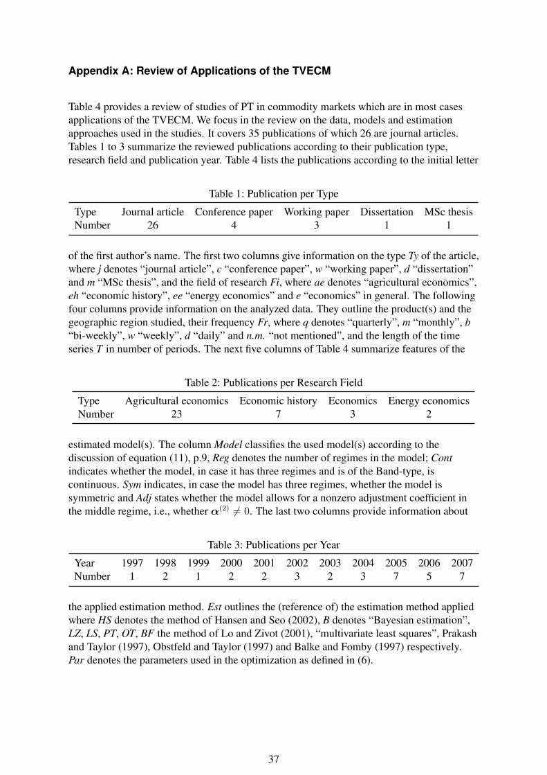
Appendix A: Review of Applications of the TVECM

Table 4 provides a review of studies of PT in commodity markets which are in most casesapplications of the TVECM. We focus in the review on the data, models and estimationapproaches used in the studies. It covers 35 publications of which 26 are journal articles.Tables 1 to 3 summarize the reviewed publications according to their publication type,research field and publication year. Table 4 lists the publications according to the initial letter

Table 1: Publication per Type

Type Journal article Conference paper Working paper Dissertation MSc thesisNumber 26 4 3 1 1

of the first author’s name. The first two columns give information on the type Ty of the article,where j denotes “journal article”, c “conference paper”, w “working paper”, d “dissertation”and m “MSc thesis”, and the field of research Fi, where ae denotes “agricultural economics”,eh “economic history”, ee “energy economics” and e “economics” in general. The followingfour columns provide information on the analyzed data. They outline the product(s) and thegeographic region studied, their frequency Fr, where q denotes “quarterly”, m “monthly”, b“bi-weekly”, w “weekly”, d “daily” and n.m. “not mentioned”, and the length of the timeseries T in number of periods. The next five columns of Table 4 summarize features of the

Table 2: Publications per Research Field

Type Agricultural economics Economic history Economics Energy economicsNumber 23 7 3 2

estimated model(s). The column Model classifies the used model(s) according to thediscussion of equation (11), p.9, Reg denotes the number of regimes in the model; Contindicates whether the model, in case it has three regimes and is of the Band-type, iscontinuous. Sym indicates, in case the model has three regimes, whether the model issymmetric and Adj states whether the model allows for a nonzero adjustment coefficient inthe middle regime, i.e., whether α(2) 6= 0. The last two columns provide information about

Table 3: Publications per Year

Year 1997 1998 1999 2000 2001 2002 2003 2004 2005 2006 2007Number 1 2 1 2 2 3 2 3 7 5 7

the applied estimation method. Est outlines the (reference of) the estimation method appliedwhere HS denotes the method of Hansen and Seo (2002), B denotes “Bayesian estimation”,LZ, LS, PT, OT, BF the method of Lo and Zivot (2001), “multivariate least squares”, Prakashand Taylor (1997), Obstfeld and Taylor (1997) and Balke and Fomby (1997) respectively.Par denotes the parameters used in the optimization as defined in (6).

37

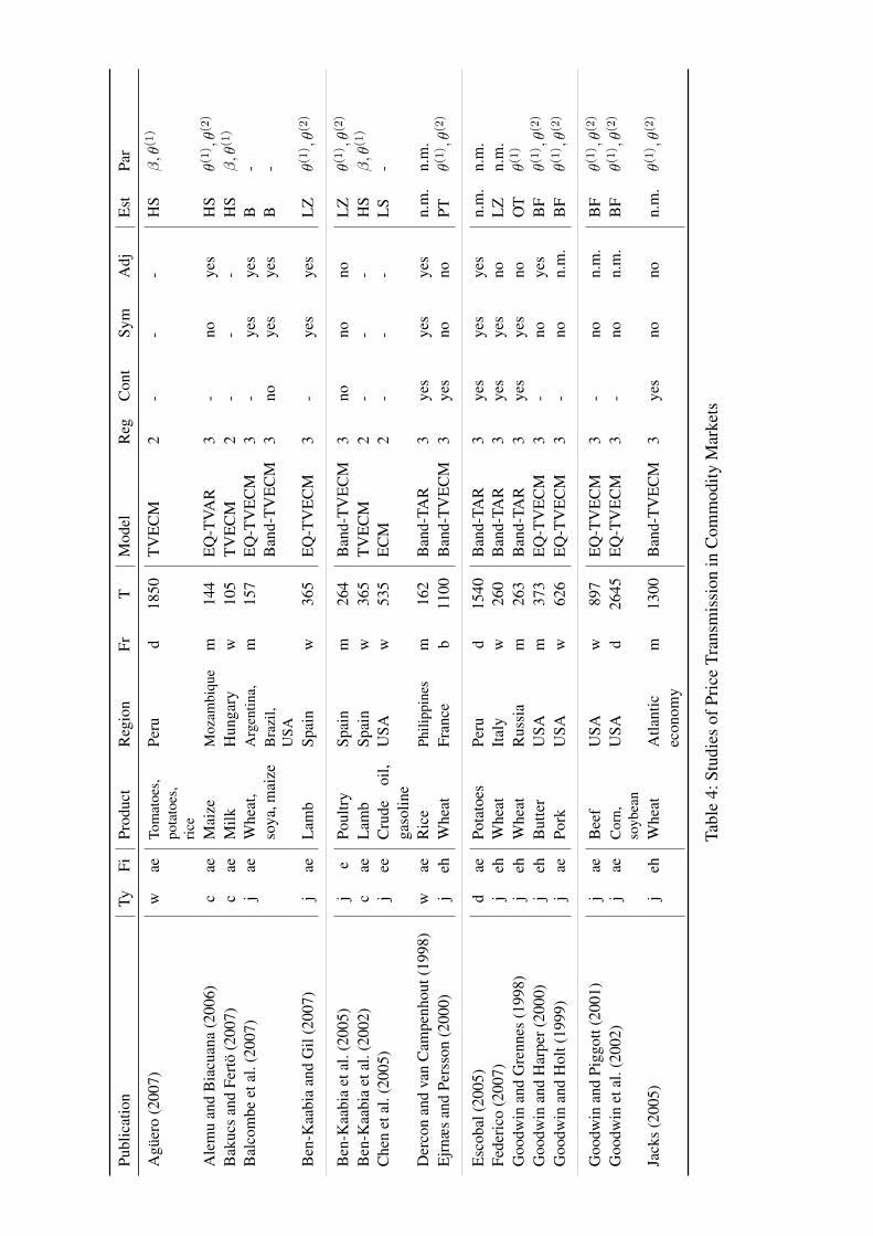
Publ

icat

ion

TyFi

Prod

uct

Reg

ion

FrT

Mod

elR

egC

ont

Sym

Adj

Est

Par

Agü

ero

(200

7)w

aeTo

mat

oes,

pota

toes

,ri

ce

Peru

d18

50T

VE

CM

2-

--

HS

β,θ

(1)

Ale

mu

and

Bia

cuan

a(2

006)

cae

Mai

zeM

ozam

biqu

em

144

EQ

-TVA

R3

-no

yes

HS

θ(1) ,θ(

2)

Bak

ucs

and

Fert

ö(2

007)

cae

Milk

Hun

gary

w10

5T

VE

CM

2-

--

HS

β,θ

(1)

Bal

com

beet

al.(

2007

)j

aeW

heat

,A

rgen

tina,

m15

7E

Q-T

VE

CM

3-

yes

yes

B-

soya

,mai

zeB

razi

l,U

SAB

and-

TV

EC

M3

noye

sye

sB

-

Ben

-Kaa

bia

and

Gil

(200

7)j

aeL

amb

Spai

nw

365

EQ

-TV

EC

M3

-ye

sye

sL

Zθ(

1) ,θ(

2)

Ben

-Kaa

bia

etal

.(20

05)

je

Poul

try

Spai

nm

264

Ban

d-T

VE

CM

3no

nono

LZ

θ(1) ,θ(

2)

Ben

-Kaa

bia

etal

.(20

02)

cae

Lam

bSp

ain

w36

5T

VE

CM

2-

--

HS

β,θ

(1)

Che

net

al.(

2005

)j

eeC

rude

oil,

gaso

line

USA

w53

5E

CM

2-

--

LS

-

Der

con

and

van

Cam

penh

out(

1998

)w

aeR

ice

Phili

ppin

esm

162

Ban

d-TA

R3

yes

yes

yes

n.m

.n.

m.

Ejr

næs

and

Pers

son

(200

0)j

ehW

heat

Fran

ceb

1100

Ban

d-T

VE

CM

3ye

sno

noPT

θ(1) ,θ(

2)

Esc

obal

(200

5)d

aePo

tato

esPe

rud

1540

Ban

d-TA

R3

yes

yes

yes

n.m

.n.

m.

Fede

rico

(200

7)j

ehW

heat

Ital

yw

260

Ban

d-TA

R3

yes

yes

noL

Zn.

m.

Goo

dwin

and

Gre

nnes

(199

8)j

ehW

heat

Rus

sia

m26

3B

and-

TAR

3ye

sye

sno

OT

θ(1)

Goo

dwin

and

Har

per(

2000

)j

ehB

utte

rU

SAm

373

EQ

-TV

EC

M3

-no

yes

BF

θ(1) ,θ(

2)

Goo

dwin

and

Hol

t(19

99)

jae

Pork

USA

w62

6E

Q-T

VE

CM

3-

non.

m.

BF

θ(1) ,θ(

2)

Goo

dwin

and

Pigg

ott(

2001

)j

aeB

eef

USA

w89

7E

Q-T

VE

CM

3-

non.

m.

BF

θ(1) ,θ(

2)

Goo

dwin

etal

.(20

02)

jae

Cor

n,so

ybea

nU

SAd

2645

EQ

-TV

EC

M3

-no

n.m

.B

Fθ(

1) ,θ(

2)

Jack

s(2

005)

jeh

Whe

atA

tlant

icec

onom

ym

1300

Ban

d-T

VE

CM

3ye

sno

non.

m.

θ(1) ,θ(

2)

Tabl

e4:

Stud

ies

ofPr

ice

Tran

smis

sion

inC

omm

odity

Mar

kets

Publ

icat

ion

TyFi

Prod

uct

Reg

ion

FrT

Mod

elR

egC

ont

Sym

Adj

Est

Par

Jack

s(2

006)

jeh

Whe

atA

tlant

icec

onom

ym

1300

Ban

d-T

VE

CM

3ye

sno

non.

m.

θ(1) ,θ(

2)

Lo

and

Ziv

ot(2

001)

je

CPI

USA

m11

5B

and-

TV

EC

M3

yes

yes

noL

Zθ(

1) ,θ(

2)

Luo

ma

etal

.(20

04)

wae

Bee

f,po

rkFi

nlan

dm

269

TV

EC

M2/

3no

/yes

-/no

-/ye

sB

-L

utz

etal

.(20

06)

jae

Mai

zeB

enin

n.m

.42

2B

and-

TV

EC

M3

yes

yes

noL

S-

Mey

er(2

004)

jae

Pork

Ger

man

y,N

ethe

rlan

dsw

600

Ban

d-T

VE

CM

3no

yes

yes

HS

θ(1)

Obs

tfel

dan

dTa

ylor

(199

7)j

eC

PIW

orld

m19

2B

and-

TV

EC

M3

yes

yes

noO

Tθ(

1)

O’C

onne

land

Wei

(200

2)j

eC

PIU

SAq

42-6

8TA

R2

--

-n.

m.

θ(1) ,d

Park

etal

.(20

07)

jee

Nat

ural

gas

Can

ada,

USA

d12

90B

and-

TV

EC

M3

nono

yes

LZ

θ(1) ,θ(

2) ,d

Pede

and

McK

enzi

e(2

005)

cae

Mai

zeB

enin

w16

2T

VE

CM

2-

--

HS

β,θ

(1)

Seph

ton

(200

3)j

aeC

orn,

soyb

ean

USA

d26

45T

VE

CM

2-

--

HS

β,θ

(1)

Serr

aan

dG

oodw

in(2

003)

jae

Dai

rySp

ain

m78

EQ

-TV

EC

M3

-no

yes

LS

θ(1) ,θ(

2)

Serr

aan

dG

oodw

in(2

004)

jae

Egg

sU

SAm

372

TV

EC

M2/

3-/

n.m

.-/

n.m

.-/

n.m

.H

Sθ(

1)

/θ(1

) ,θ(

2)

Serr

a,G

ilet

al.(

2006

)j

aePo

rkD

enm

ark,

Fran

ce,

Ger

man

y,Sp

ain

w57

4E

Q-T

AR

3-

noye

sB

Fθ(

1) ,θ(

2)

Serr

a,G

oodw

inet

al.(

2006

)j

aeE

ggs

USA

m36

0E

Q-T

AR

3-

noye

sn.

m.

θ(1) ,θ(

2)

Tren

kler

and

Wol

f(20

05)

jeh

Whe

atflo

urPo

land

m19

0B

and-

TAR

3ye

sye

sno

LZ

n.m

.

Uch

ezub

a(2

005)

mae

App

les

Sout

hA

fric

am

148

Ban

d-T

VE

CM

3no

noye

sL

Zθ(

1) ,θ(

2)

Van

Cam

penh

out(

2007

)j

aeM

aize

Tanz

ania

w62

6E

Q-T

AR

3-

yes

non.

m.

θ(1) ,θ(

2)

Tabl

e4:

Stud

ies

ofPr

ice

Tran

smis

sion

inC

omm

odity

Mar

kets

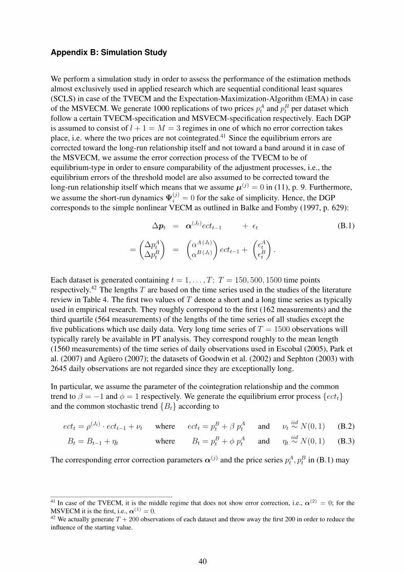
Appendix B: Simulation Study

We perform a simulation study in order to assess the performance of the estimation methodsalmost exclusively used in applied research which are sequential conditional least squares(SCLS) in case of the TVECM and the Expectation-Maximization-Algorithm (EMA) in caseof the MSVECM. We generate 1000 replications of two prices pAt and pBt per dataset whichfollow a certain TVECM-specification and MSVECM-specification respectively. Each DGPis assumed to consist of l + 1 = M = 3 regimes in one of which no error correction takesplace, i.e. where the two prices are not cointegrated.41 Since the equilibrium errors arecorrected toward the long-run relationship itself and not toward a band around it in case ofthe MSVECM, we assume the error correction process of the TVECM to be ofequilibrium-type in order to ensure comparability of the adjustment processes, i.e., theequilibrium errors of the threshold model are also assumed to be corrected toward thelong-run relationship itself which means that we assume µ(j) = 0 in (11), p. 9. Furthermore,we assume the short-run dynamics Ψ

(j)i = 0 for the sake of simplicity. Hence, the DGP

corresponds to the simple nonlinear VECM as outlined in Balke and Fomby (1997, p. 629):

∆pt = α(Jt)ectt−1 + εt (B.1)

=

(∆pAt∆pBt

)=

(αA (Jt)

αB (Jt)

)ectt−1 +

(εAtεBt

).

Each dataset is generated containing t = 1, . . . , T ; T = 150, 500, 1500 time pointsrespectively.42 The lengths T are based on the time series used in the studies of the literaturereview in Table 4. The first two values of T denote a short and a long time series as typicallyused in empirical research. They roughly correspond to the first (162 measurements) and thethird quartile (564 measurements) of the lengths of the time series of all studies except thefive publications which use daily data. Very long time series of T = 1500 observations willtypically rarely be available in PT analysis. They correspond roughly to the mean length(1560 measurements) of the time series of daily observations used in Escobal (2005), Park etal. (2007) and Agüero (2007); the datasets of Goodwin et al. (2002) and Sephton (2003) with2645 daily observations are not regarded since they are exceptionally long.

In particular, we assume the parameter of the cointegration relationship and the commontrend to β = −1 and φ = 1 respectively. We generate the equilibrium error process ecttand the common stochastic trend Bt according to

ectt = ρ(Jt) · ectt−1 + νt where ectt = pBt + β pAt and νtiid∼ N(0, 1) (B.2)

Bt = Bt−1 + ηt where Bt = pBt + φ pAt and ηtiid∼ N(0, 1) (B.3)

The corresponding error correction parameters α(j) and the price series pAt , pBt in (B.1) may

41 In case of the TVECM, it is the middle regime that does not show error correction, i.e., α(2) = 0; for theMSVECM it is the first, i.e., α(1) = 0.42 We actually generate T + 200 observations of each dataset and throw away the first 200 in order to reduce theinfluence of the starting value.

40

then be calculated based on the generated values of ectt and Bt in via the identities

pAt =Bt − ecttφ− β

pBt =φ · ectt − βBt

φ− β

αA (j) =1− ρ(j)

φ− βαB (j) = −φ(1− ρ(j))

φ− β.

We generate datasets for the four cases in Table 6, p. 43. In cases I and IV, we are interestedin the performance of the estimation methods depending on the true parameters introducingnonlinearity, i.e., the thresholds and the transition matrix.43 Hence, we focus on theestimation of the thresholds and the ergodic probabilities in dependence on a set of varyingtrue thresholds and ergodic probabilities incorporating the error correction parameter as anuisance parameter in order to study if and to what extent they influence the estimationresults.44 The parameters varied in the DGPs of the TVECM and the MSVECM are thethresholds θ(1), θ(2) and the error correction parameters ρ(1), ρ(3) of the outer regimes and theergodic probabilities π(2), π(3) and the error correction parameters ρ(1), ρ(3) respectively.45

As criterion measuring the performance of the estimation of the thresholds via SCLS and theergodic probabilities via EMA we choose the mean squared error

MSEλ = E(λ− λ)2 =[Bias(λ)

]2+ σ2(λ). Hence, the MSE of SCLS is estimated for

λ ∈ θ(1), θ(2) and the MSE of the EMA for λ ∈ , π(1), π(2), π(3). We approximate thefunctional relationship between the MSE and the varying true parameters of the DGPs by

MSEλ =

[Bias(λ)

]2

+ σ2(λ). The evaluation of MSESCLSλ

= f(θ(1), θ(2), ρ(1), ρ(3)) and

MSEEMAλ

= f(π(2), π(3), ρ(1), ρ(3)) for grids of true parameters is first computationally verydemanding and can hardly graphically be illustrated due to its five dimensions. We thusreduce the number of dimensions to three by evaluating the MSE function by holding its thirdand fourth parameters constant MSEA

λ= f(θ(1), θ(2)|ρ(1), ρ(3)),

MSECλ

= f(π(2), π(3)|ρ(1), ρ(3)) ) and evaluating it by holding its first and second parametersconstant (MSEB

λ= f(ρ(1), ρ(3)|θ(1), θ(2)), MSED

λ= f(ρ(1), ρ(3)|π(2), π(3)) ) respectively.

Despite we restrict the simulation on these two subspaces, detailed insights into the behaviorof the estimation methods can be expected.

43 Since the transition matrix of the MSVECM-DGP considered contains nine elements, we use the three cor-responding ergodic probabilities π = (π(1) π(2) π(3))> instead. These are, technically spoken, the normalizedeigenvector of the matrix associated with its unit eigenvalue (cf. Hamilton, 1994, pp. 681). The transition matrixand the ergodic probabilities are connected via Γ = TΛT−1 (Hamilton, 1994, p. 730) where T is the M ×Mmatrix of the eigenvectors and Λ the M ×M diagonal matrix of the eigenvalues of Γ. Hence, by holding all ele-ments of Λ constant and only plugging in varying π in the column of T associated with the unit eigenvalue, thecorresponding transition matrices can be obtained. The ergodic probabilities corresponding to an estimated tran-sition matrix Γ can be obtained, in turn, by the eigenvalue decomposition of the latter and normalization of the

respective eigenvector. We obtained Λ and T from the eigenvalue decomposition of Γ =

0.95 0.03 0.020.15 0.8 0.050.2 0.1 0.7

since it implies ergodic probabilities of π = (0.769 0.154 0.077)>, i.e., it assigns quite distinct unconditionalprobabilities to the three regimes.44 Since we simulate according to (B.2) and (B.3), we vary the autoregressive parameter ρ(j) in (B.2) instead ofα(j).45 Note thatα(2) = 0 implying that ρ(2) = 1 in both cases and π(1) = 1−(π(2)+π(3)). As mentioned before, theergodic probabilities denote the expected unconditional probabilities π(j) of the j = 1, . . . ,M ; M = 3 regimes.The frequencies of the regimes generated by a MSVECM-DGP should hence equal them asymptotically.

41

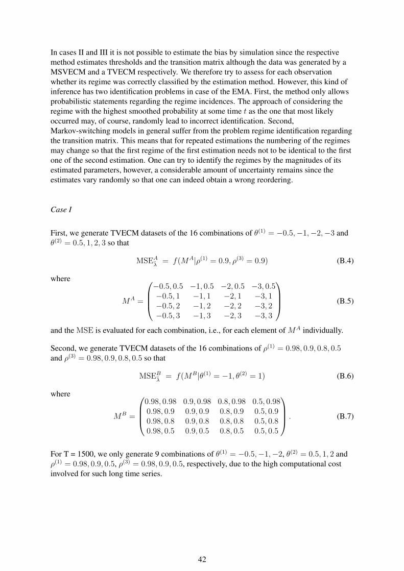
In cases II and III it is not possible to estimate the bias by simulation since the respectivemethod estimates thresholds and the transition matrix although the data was generated by aMSVECM and a TVECM respectively. We therefore try to assess for each observationwhether its regime was correctly classified by the estimation method. However, this kind ofinference has two identification problems in case of the EMA. First, the method only allowsprobabilistic statements regarding the regime incidences. The approach of considering theregime with the highest smoothed probability at some time t as the one that most likelyoccurred may, of course, randomly lead to incorrect identification. Second,Markov-switching models in general suffer from the problem regime identification regardingthe transition matrix. This means that for repeated estimations the numbering of the regimesmay change so that the first regime of the first estimation needs not to be identical to the firstone of the second estimation. One can try to identify the regimes by the magnitudes of itsestimated parameters, however, a considerable amount of uncertainty remains since theestimates vary randomly so that one can indeed obtain a wrong reordering.

Case I

First, we generate TVECM datasets of the 16 combinations of θ(1) = −0.5,−1,−2,−3 andθ(2) = 0.5, 1, 2, 3 so that

MSEAλ

= f(MA|ρ(1) = 0.9, ρ(3) = 0.9) (B.4)

where

MA =

−0.5, 0.5 −1, 0.5 −2, 0.5 −3, 0.5−0.5, 1 −1, 1 −2, 1 −3, 1−0.5, 2 −1, 2 −2, 2 −3, 2−0.5, 3 −1, 3 −2, 3 −3, 3

(B.5)

and the MSE is evaluated for each combination, i.e., for each element of MA individually.

Second, we generate TVECM datasets of the 16 combinations of ρ(1) = 0.98, 0.9, 0.8, 0.5and ρ(3) = 0.98, 0.9, 0.8, 0.5 so that

MSEBλ

= f(MB|θ(1) = −1, θ(2) = 1) (B.6)

where

MB =

0.98, 0.98 0.9, 0.98 0.8, 0.98 0.5, 0.980.98, 0.9 0.9, 0.9 0.8, 0.9 0.5, 0.90.98, 0.8 0.9, 0.8 0.8, 0.8 0.5, 0.80.98, 0.5 0.9, 0.5 0.8, 0.5 0.5, 0.5

. (B.7)

For T = 1500, we only generate 9 combinations of θ(1) = −0.5,−1,−2, θ(2) = 0.5, 1, 2 andρ(1) = 0.98, 0.9, 0.5, ρ(3) = 0.98, 0.9, 0.5, respectively, due to the high computational costinvolved for such long time series.

42

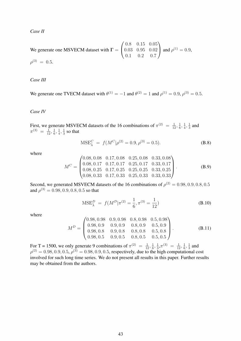
Case II

We generate one MSVECM dataset with Γ =

0.8 0.15 0.050.03 0.95 0.020.1 0.2 0.7

and ρ(1) = 0.9,

ρ(3) = 0.5.

Case III

We generate one TVECM dataset with θ(1) = −1 and θ(2) = 1 and ρ(1) = 0.9, ρ(3) = 0.5.

Case IV

First, we generate MSVECM datasets of the 16 combinations of π(2) = 112, 1

6, 1

4, 1

3and

π(3) = 112, 1

6, 1

4, 1

3so that

MSECλ

= f(MC |ρ(2) = 0.9, ρ(3) = 0.5). (B.8)

where

MC =

0.08, 0.08 0.17, 0.08 0.25, 0.08 0.33, 0.080.08, 0.17 0.17, 0.17 0.25, 0.17 0.33, 0.170.08, 0.25 0.17, 0.25 0.25, 0.25 0.33, 0.250.08, 0.33 0.17, 0.33 0.25, 0.33 0.33, 0.33

. (B.9)

Second, we generated MSVECM datasets of the 16 combinations of ρ(2) = 0.98, 0.9, 0.8, 0.5and ρ(3) = 0.98, 0.9, 0.8, 0.5 so that

MSEDλ

= f(MD|π(2) =1

6, π(3) =

1

12) (B.10)

where

MD =

0.98, 0.98 0.9, 0.98 0.8, 0.98 0.5, 0.980.98, 0.9 0.9, 0.9 0.8, 0.9 0.5, 0.90.98, 0.8 0.9, 0.8 0.8, 0.8 0.5, 0.80.98, 0.5 0.9, 0.5 0.8, 0.5 0.5, 0.5

. (B.11)

For T = 1500, we only generate 9 combinations of π(2) = 112, 1

6, 1

3,π(3) = 1

12, 1

6, 1

3and

ρ(2) = 0.98, 0.9, 0.5, ρ(3) = 0.98, 0.9, 0.5, respectively, due to the high computational costinvolved for such long time series. We do not present all results in this paper. Further resultsmay be obtained from the authors.

43

Table 5: Estimation Approaches of Selected Publications46

Publication Model l d Principle Criterion Par’s Optim.

Balke and Fomby (1997) SETAR any est. LS RSS θ, d MinObstfeld and Taylor (1997) SETAR 147 1 ML LR48 θ MaxHansen (1999) SETAR 0-2 est. LS RSS θ, d MinLo and Zivot (2001) TVECM 1 est. LS RSS θ, d MinHansen and Seo (2002) TVECM 1 1 ML log |Σ| θ, β Min

Table 6: Design of the Simulation Study

Estimation DGPTVECM MSVECM

SCLS I IIEMA III IV

Table 7: True vs. Estimated Regime Incidences (Case II)

R1 true R2 true R3 true

R1 est 0.339 0.076 0.041R2 est 0.216 0.039 0.018R3 est 0.214 0.039 0.019

Table 8: True vs. Estimated Regime Incidences (Case III)

R1 true R2 true R3 true

R1 est 0.088 0.105 0.028R2 est 0.133 0.152 0.044R3 est 0.186 0.199 0.065

46 Obstfeld and Taylor estimate a symmetric TVECM(3), i.e. in absolute terms, only one symmetric threshold isto be estimated.47 LR denotes the likelihood ratio between a SETAR(3,1,1,1) and an AR(1). The latter model might also be calleda SETAR (1,1), for the notation of SETAR models see footnote 6, p. 4.48 l denotes the number of thresholds (compare footnote 18, page 8), d the delay parameter, ML maximum like-lihood, LS least squares, RSS = trace(Σ) residual sum of squares, log |Σ| the log determinant of the variance-covariance matrix of the residuals; θ means threshold, est. estimated and β the cointegration vector.

44

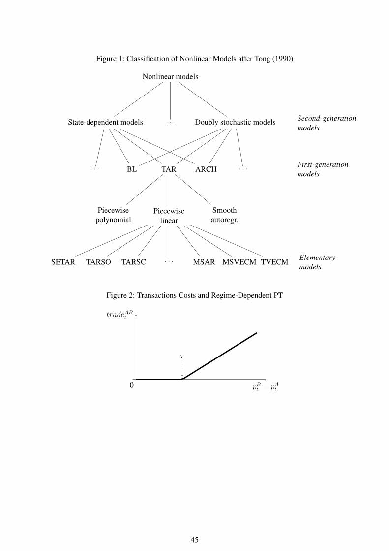
Figure 1: Classification of Nonlinear Models after Tong (1990)

Nonlinear models

State-dependent models . . . Doubly stochastic models

. . . BL TAR

Piecewisepolynomial

Piecewiselinear

SETAR TARSO TARSC . . . MSAR MSVECM TVECM

Smoothautoregr.

ARCH . . .

Second-generationmodels

First-generationmodels

Elementarymodels

Figure 2: Transactions Costs and Regime-Dependent PT

pBt − pAt

tradeABt

τ

0

45

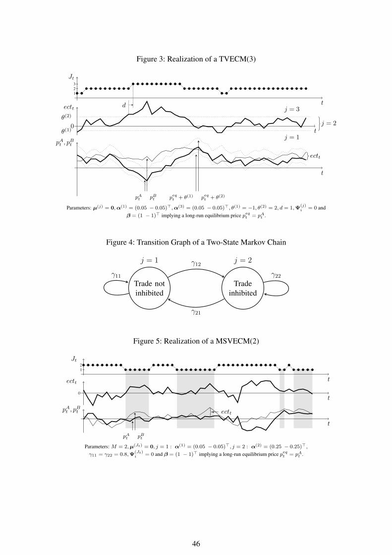
Figure 3: Realization of a TVECM(3)

t

pAt , pBt

0t

ectt

θ(1)

θ(2)j = 2

j = 1

j = 3t

Jt

123

d

ectt

pAt pB

t peqt + θ(1) peq

t + θ(2)

Parameters: µ(j) = 0,α(1) = (0.05 − 0.05)>,α(3) = (0.05 − 0.05)>, θ(1) = −1, θ(2) = 2, d = 1,Ψ(j)i = 0 and

β = (1 − 1)> implying a long-run equilibrium price peqt = pA

t .

Figure 4: Transition Graph of a Two-State Markov Chain

Trade notinhibited

j = 1

Tradeinhibited

j = 2

γ11

γ12

γ22

γ21

Figure 5: Realization of a MSVECM(2)

t

pAt , pBt

0

t

ectt t

Jt

12

ectt

pAt pB

t

Parameters: M = 2,µ(Jt) = 0, j = 1 : α(1) = (0.05 − 0.05)>, j = 2 : α(2) = (0.25 − 0.25)>,

γ11 = γ22 = 0.8,Ψ(Jt)i = 0 and β = (1 − 1)> implying a long-run equilibrium price peq

t = pAt .

46

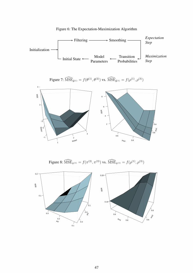
Figure 6: The Expectation-Maximization Algorithm

Filtering Smoothing

TransitionProbabilities

ModelParameters

Initial State

Initialization

ExpectationStep

MaximizationStep

Figure 7: MSEθ(1) = f(θ(1), θ(2)) vs. MSEθ(1) = f(ρ(1), ρ(3))

theta1

−3

−2

−1

theta21

2

3

MS

E

2

3

rho1

0.6

0.8

rho3

0.6

0.8

MS

E

2

4

6

8

Figure 8: MSEπ(1) = f(π(2), π(3)) vs. MSEπ(1) = f(ρ(1), ρ(3))

pi2

0.1

0.2

0.3

pi3

0.1

0.2

0.3

MS

E

0.1

0.2

rho1

0.6

0.8

rho3

0.6

0.8

MS

E

0.15

0.20

47