a comparison of yield estimation techniques for
TRANSCRIPT

\A COMPARISON OF YIELD ESTIMATION TECHNIQUES FOR
OLD-FIELD LOBLOLLY PINE PLANTATION~1
by
Mike Robert ,,Strubl
Dissertation submitted to the Graduate Faculty of
the Virginia Polytechnic Institute and State University
in partial fulfillment of the requirements for the degree of
DOCTOR OF PHILOSOPHY
in
Statistics
APPROVED:
W. R. Pirie, Co-chairman H. E. Burkhart, Co-chairman
0 J. C. Arnold •
M. R. Reynolds
R. B. Vasey
June, 1976 Blacksburg, Virginia

ACKNOWLEDGEMENTS
I wish to express my sincere appreciation to my
committee for their helpful guidance, encouragement, and
interest: Dr. Walter R. Pirie, Dr. Harold E. Burkhart,
Dr. Richard B. Vasey, Dr. Marion R. Reynolds, and
Dr. Jesse C. Arnold. Especially, I wish to thank my
co-chairmen, Dr. Pirie and Dr. Burkhart, who guided me
throughout the study.
I wish to thank the Division of Forestry and
Wildlife Resources for providing teaching and research
assistantships and an instructorship which made it
possible for me to continue my studies.
I wish to thank my parents for encouragement and
financial assistance.
Finally, I wish to thank my wife, Sue, for her
patience, inspiration and for typing this dissertation.
ii
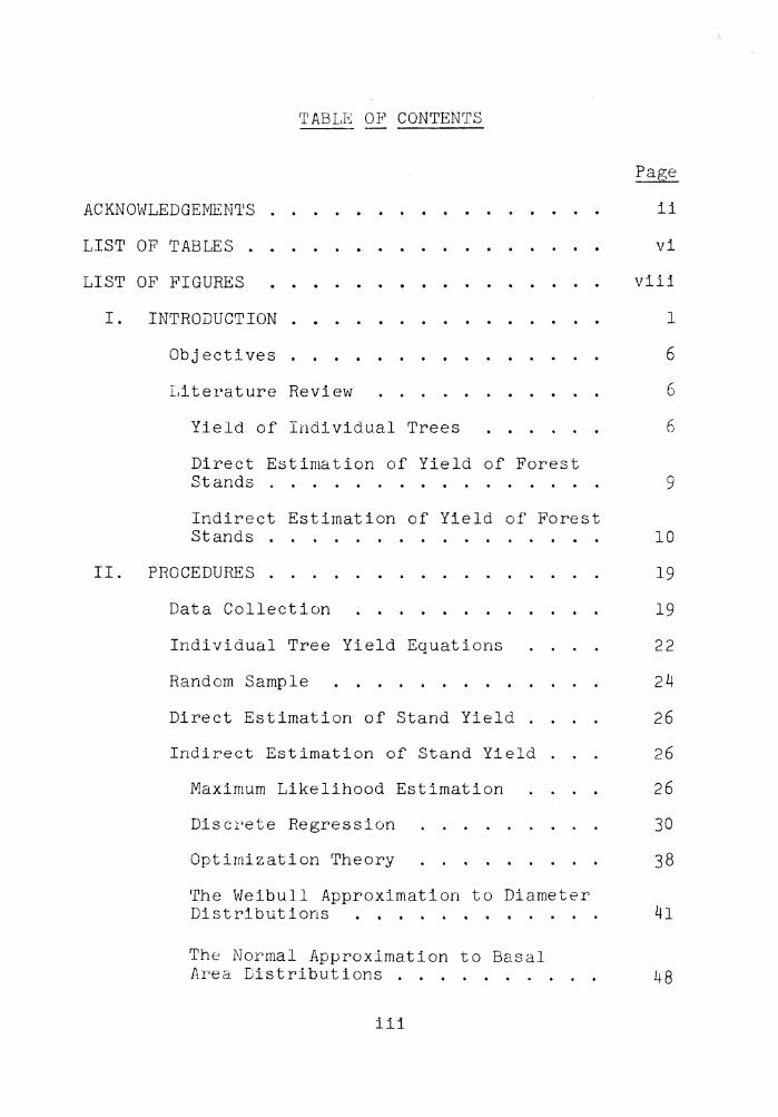
TABLE OF CONTENTS
ACKNOWLEDGEMENTS
LISIJ1 OF TABLES . . . . . . . . . . . . . . . LIST OF FIGURES
I. INTRODUCTION .
Objectives
Literature Review
Page
ii
vi
viii
1
6
6
Yield of Individual Trees 6
Direct Estimation of Yield of Forest Stands . . . . . . . . . . . 9
Indirect Estimation of Yield of Forest Stands . . . . . . . . . 10
II. PROCEDURES .
Data Collection
Individual Tree Yield Equations
Random Sample
Direct Estimation of Stand Yield
Indirect Estimation of Stand Yield
Maximum Likelihood Estimation
Discrete Regression
Optimization Theory
The Weibull Approximation to Diameter
19
19
22
24
26
26
26
30
38
Distributions . . . . . . . . 41
The Normal Approximation to Basal Area Distributions . . . . . . 48
iii

iv
The Transformed Normal Approximation to Basal Area Distributions . . . .
A Discrete Approximation to Diameter Distributions . . . . . . . . . .
Prediction of Yield from the Estimated Diameter Distribution . . . . . . . .
Comparison Techniques for Evaluating Yield Prediction . . . . . .
Kolmogorov-Smirnov Tests . .
Comparison of Observed and Estimated
50
5(
62
76
76
Yields . . . . . . . . . . . . . 83
Comparison of Culmination of Mean Annual Increment . . . . . . 84
III. RESUL'l'S AND DISCUSSION .
Kolmogorov-Smirnov Tests .
Comparison of Observed and Estimated
87
87
Yields . . . . . . . . . . . . . 90
Comparison of Culmination of Mean Annual Increment . . . . . . . . . . . . . 95
IV. A UNIFIED APPROACH TO YIELD PREDICTION 106
The Differential Equation Approach . . 106
Past Application of Differential Equation Models to Growth and Yield Prediction . . . . . . . . . . . . 110
A Stochastic Approach to Modeling of Growth and Yield . . . . . . . . . . 113
Derivation of the Transformed Normal Diameter Distribution . . . . . . 117
A Stochastic Model for Open-Grown Loblolly Pine . . . . . . 119
Stochastic Modeling of Stand-Grown Trees 135

v
Effective Crown Area ..
Photosynthate Allocation
A Description of Basal Area Growth
Page
136
142
in Stand-Grown Trees . . . . . . 144 Estimation of Distributions and Parameters in the Basal Area-Height Model . . . . . . . . . 149 Application of the Basal Area-Height Model to Estimation of Yields of Forest Stands . . . . . . . . . . . 151
V. CONCLUSIONS AND RECOMMENDATIONS 156
161
168
LITERATURE CITED
VITA

•rable
2.1
2.2
2.3
2.4
2.5
3.1
3.2
3.3
3.4
LIST OF TABLES
Coefficients of individual tree volume equations . . . . . . . . . . . . . .
Parameter estimates, coefficients of determination, and standard errors of esti-mate for per-acre yield prediction via the direct yield estimation approach for 136 sample plots in loblolly pine plantations . .
Parameter estimates, coefficients of determination, and standard errors of esti-mate for prediction of quantiles and minimum and average diameters on 0.1-acre plots in loblolly pine stands . . . . . . . .
A comparison of three tests for normality from the simulation of 1000 standard normal samples of size 80 . . . . . . . . . . . . .
A comparison of tests for normality of tree basal areas on 186 sample plots from old-fie ld loblolly pine plantations . . . . . . .
Frequency of rejection for Kolmogorov-Smirnov tests comparing estimated and observed diameter distribution on the 50 randomly selected plots .......... .
Means and variances of differences between observed and estimated yields on 50 randomly selected plots . . . . . . . . . . . . . . .
Age at which mean annual increment culminates for various site index and initial density combinations when yields are estimated directly from stand variables via multiple regression equation (1.4) ......... .
Age at which mean annual increment culminates for various site index and initial density combinations when yields are estimated indirectly with the Weibull distribution function, quantile approach to yield estima-tion, and 1-inch class interval yield estima-tion procedure . . . . . . . . . . . . . . .
vi
25
27
46
80
81
91
99
vii
Table
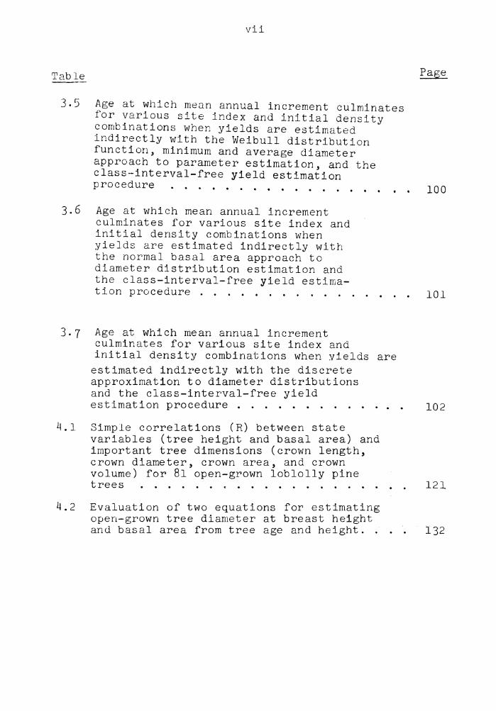
3.5 Age at which mean annual increment culminates for various site index and initial density combinations when yields are estimated indirectly with the Weibull distribution function, minimum and average diameter approach to parameter estimation, and the class-interval-free yield estimation procedure . . . . . . . . . . . . . . . . • , 100
3.6 Age at which mean annual increment culminates for various site index and initial density combinations when yields are estimated indirectly with the normal basal area approach to diameter distribution estimation and the class-interval-free yield estima-tion procedure . . . . . . . .
3.7 Age at which mean annual increment culminates for various site index and initial density combinations when vields are
estimated indirectly with the discrete approximation to diameter distributions and the class-interval-free yield
101
estimation procedure . . . . . . . . . . . 102
4.1 Simple correlations (R) between state variables (tree height and basal area) and important tree dimensions (crown length, crown diameter, crown area, and crown volume) for 81 open-grown loblolly pine trees . . c • • • • • • • • • • • 121
4.2 Evaluation of two equations for estimating open-grown tree diameter at breast height and basal area from tree age and height. . 132

LIST OF FIGURES
Figure
4.1 The relationship between height and age, and least squares fit for 81 open-grown loblolly pine trees . . . . . . . . . 123
4.2 The relationship between crown length and height and least squares fit for 81 open-grown loblolly pine trees . . . . . . 124
4.3 The relationship between crown length and height, and least squares fit for 477 stand-grown loblolly pine trees . . . . . . 126
4.4 The relationship between crown width and height, and least squares fit for 81 open-grown loblolly pine trees . . . . 130
4.5 The relationship between crown area and the square of height, and least squares fit for 81 open-grown loblolly pine trees . . . . 140
viii
-
I. INTRODUCTION
Loblolly pine (Pinu~ taeda) is a fast growing
species that is intensively managed for the production
of pulpwood, sawlogs, and veneer bolts. High early return
on investments (when compared with returns from growth of
other species) justifies the large monetary investments
required for intensive management. A fundamental require-
ment of most management systems is yield information.
Sophisticated management planning aids such as RETURN
(Schweitzer et al., 1967), TEVAP 2 (Myers, 1973) and
TIMBER RAM (Navon, 1971) require detailed and accurate
yield projections. Yield information is also required
for computer simulations such as the Purdue Management
Game (Bare, 1970), used to train forest managers.
The topic of this dissertation is the development
of quantative models to supply forest managers with
yield estimates fundamental to long range planning. Yield
is defined as the amount of wood produced by a collection
or stand of trees over some time period. The units in
which yield is measured are determined by the product which
is to be manufactured from the trees. Volume or weight of
solid wood contained in the bole of the trees is the
common unit of measure when paper is produced from the
trees. Larger trees are often measured according to the
1
2
amount of lumber which can be manufactured from them.
The unit of measure for lumber is termed the board foot,
defined as 144 cubic inches. Specific models for yield
estimation will be discussed later in this chapter and
in Chapters 2 and 4. A general description of the
derivation of yield models follows.
The yield of a stand of trees depends on the
genetic make-up of the trees, the environmental conditions
to which the trees are exposed, and the length of time
over which the trees are grown. Only a few of these
factors have been successfully quantified. For example.,
genetic make-up of trees is currently under extensive
research and an issue of considerable debate; accurate
measurement of this factor has not been included in
previous growth models. In conventional yield models
environmental conditions are commonly described by two
quantities -- one a measure of the growing quality of
the land upon which the trees are planted, the second an
indication of the competition between trees for scarce
resources. A third factor that is usually included in
yield models is the length of time over which the trees
are grown. These three quantifiable variables are termed
stand variables. In this stud~ the measure of site quality
is site index, the indicator of competition between trees
is the number of trees per acre, and the length of time
the trees are grown is stand age.
3
Site index is a measure of the fertility of the
land upon which the trees are planted. It is defined
as the average height of the largest trees in the stand
at some base age, usually 25 years for loblolly pine
plantations. Site index curves can be constructed by
assuming the following functional relationship between
stand age (A) and the average height of the largest
trees (Hd):
(1.1)
The expression log10 (.) indicates the base 10 logarithm
of the argument. Site index is estimated from a single
observation of the age and average height of the largest
trees. Yield is often predicted as a function of
estimated site index plus other variables. An alternate
approach to using site index is to predict yield from Hd,
since stand age is also included in both yield and site
prediction schemes. The stand variable Ha is often
preferred since it is measured, not estimated as is site
index.
The second stand variable is the number of trees
per acre (N) in the plantation. Increasing N at a fixed
age and site index results in increasing competition for
scarce resources. Increasing A and holding N fixed also
results in increasing competitive stress. Competition is
a function of N, A, and site index.
4
A yield equation is a function used to pr~dict yield
from the stand variables Hd' N, and A. Two types of yield
estimation techniques will be discussed in this presenta-
tion, they will be labeled direct and indirect methods.
Direct yield estimation methods relate stand yield
directly to stand variables. A common procedure is to use
stepwise r·egression to obtain a functional form and to
estimate coefficients. This technique makes little or
no use of knowledge of fundamental physical and biological
processes which result in the yield of a stand of trees.
Indirect yield processes which result in yield production
techniques are based on rudimentary processes which result
in yield production. The characteristic process of yield
formation upon which indirect techniques are based is that
the yield of a stand of trees is the summation of the
yield of the individual trees in the stand. Other
physiological processes may inspire the choice of the
functional form used to model individual tree yield.
The purpose of this dissertation is to critically
examine direct and indirect yield prediction procedures
currently in use, and to suggest new yield prediction
procedures which may be superior to those currently in
use. Yield prediction models can be compared on several
levels. One criterion of the worth of a model is the
accuracy and precision of estimates obtained from
the model. The manager is most concerned about this
5
criterion. He is interested in obtaining an accurate
estimate of .the yield at the end of some growth period
so that he can pursue a course of action which is
financially rewarding and ecologically sound. A second
criterion, also of concern to the manager, is the amount
of detail contained in the yield information. Direct
yield prediction models supply only a total stand yield
estimate. Indirect yield techniques supply detailed
information related to the size and yield of individual
trees. This information is useful in making management
decisions such as determining optimal harvesting methods.
A third criterion is the biological relevance of the yield
prediction model. This criterion is of lesser importance
to the forest manager. The manager is satisfied if the
yield model conforms to certain pre-conceived notions
of tree growth (e.g. the age at which mean annual increment
should culminate). While these notions are of some
consequence, other biological factors seldom referenced
by forest managers should form the basis of yield predic-
tion models. The importance of biological factors is
supported by the following argument.
Most yield prediction models are functionally
derived from a single data set. Extrapolation of such
models outside the range of observed values in the original
data set is dangerous. Another approach is to base the
functional form of yield equations on the biological
6
processes which produce yield. This approach should
~uggest a model which is less sensitive to pecularities
of the data set.
Objectives
The objectives for this dissertation were: (1) to
compare existing yield prediction techniques in light
of information required for forest management, (2) to
suggest possible improvement of existing techniques
espectially improvements based on biological and physiolog-
ical aspects of yield production, and (3) to derive new
yield prediction techniques based on biological and
physiological aspects of yield production.
Literature Review
Yield of Individual Trees
The data base used to construct direct and indirect
yield equations depends on individual tree yield equations.
Direct determination of the yield of a large number of
trees is prohibitively expensive. Instead individual tree
data are collected and tree yield is predicted from the
easily measured variables, tree diameter at breast height
(Dor dbh) and total tree height (H). The prediction
equations developed are used to estimate the yield of
trees by measuring only D and H for each tree. Individual
tree height, ~is more difficult to measure than D and
7
further reduction in the cost of data collection is
achieved by predicting individual tree volume from
D alone or from D and other stand variables. A
general treatment of individual tree volume equations
is given in Chapter 9 of Hush et al. (1972), and
Chapters 4 to 9 of Spurr (1952).
Yield of individual trees varies according to the
product which is to be manufactured from the tree. In
general tree yield is proportional to the volume of the
bole of the tree. Tree boles assume geometric shapes
similar to cylinders, cones, paraboloids, and neiloids.
In each case listed above the volume of the figure is
proportional to the product of the area of the base and
the height. Analogously total volume of a tree bole
should be approximately proportional to the product of
the square of diameter at breast height and total tree
height. The equation which describes the relationship,
(1.2)
has been labelled the constant form factor volume equation.
The constant form factor volume equation must be
modified to provide accurate estimation of the yield of
products such as lumber. The top-most section of the
tree bole, often referred to as topwood, cannot be
economically utilized. The point beyond which the bole
of the tree cannot be used for manufacture of a product is
8
termed the merchantability limit. This merchantability
limit is usually the point on the tree where some minimum
diameter is reached. In this case the yield of the tree
is proportional to the volume of the bole excluding the
topwood, or the volume of the tree up to the merchant-
ability limit. The combined variable volume equation,
( 1. 3)
is commonly used to model tree volume to some merchantability
limit. Equation (1.2) is a special case of (1.3), with
B0 equal to 0. The intercept, B0 , is negative and
represents loss of volume due to topwood. This loss in
volume should be constant since the area of the base
of the topwood is constant, and, if all trees taper at the
same rate, the height of the topwood will be constant.
Although many other functional forms have been considered,
the combined variable is the most common functional form.
This equation was used by Burkhart et al. ( 1972) to
predict the yield of individual trees found in loblolly
pine plantations.

9
Direct Estimation of Yield of Forest Stands
The initial step in the implementation of this
procedure is data collection. Some subset of the trees
in a forest stand is chosen for measurement, usually all
the trees on some fraction of an acre of land. The
stand variables are measured for this subset of the
stand. Average yield per acre in the stand is estimated
by (1) estimating the yield of each tree in the subset
according to the technique described in the preceding
section, (2) summing individual tree yield to obtain an
estimate of the yield of the trees on that fractional
part of an acre, and (3) multiplying by some constant to
convert the yield estimate to yield per acre.
Multiple regression is then applied to the data
described above. The dependent variable is
yield per acre or some transformation of yield
per acre. The independent variables are the stand
variables and functions of the stand variables. A
stepwise procedure is often used to aid in the determina-
tion of the proper functional form of the yield predic-
tion equation. Yield prediction is described in detail in
Chapters 17, 18, 21 and 22 of Spurr (1952), and in
Chapter 17 of Hush et al. (1972).
Burkhart et al. (1972) computed yield equations for
loblolly pine plantat;ons; multiple regression was used

10
to estimate average stand yield per acre (Y),
This equation was used to estimate stand yield per acre
for cubic feet of wood contained in the boles of the
trees to various merchantability limits and for board
feet contained in the boles of the trees.
When lumber is cut from the tree bole, the topwood
can be used in the manufacture of paper. Burkhart et
al. (1972) developed a different functional form to
estimate the volume of topwood (CV2 ) from the board foot
volume per acre estimate (BF) and the cubic foot volume
per acre estimate (CV1 ) obtained from (1.4),
( 1. 5)
resulting in
( 1. 6)
Indirect Estimation of Yield of Forest Stands
One indirect method of yield estimation is referred
to in the forestry literature as the diameter distribution
method. Stand yield estimates are obtained by first
estimating the frequency distribution of tree diameters
at breast height of the trees in the stand. The estimated
frequency distributi.on, height prediction equations, and
11
individual tree yield equations are used to predict
stand yield.
The frequency distribution of tree diameters has
been studied since the late eighteen hundreds. Meyer
(1930) summarized these early attempts to describe
diameter distributions. Graphical techniques suggested
by Bruce and Reineke (1928) consisted of fitting the
normal or log-normal distribution to the data by using
special graph paper. Parameters were estimated by
drawing a straight line through the center of the data
points. Other techniques for estimating parameters
suggested by early researchers were based on the method
of moments. Meyer (1928) used Charlier curves to describe
diameter distributions by equating the coefficient of
asymmetry and the coefficient of excess of the data to
that of the Charlier curve. Schnur (1934) used Charlier
curves and Pearson curves to approximate the diameter
distribution of old-field loblolly pine stands. Osborne
and Schumacher (1935) used the Pearl-Reed growth curve (a
generalized form of the logistic distribution) to describe
the diameter distribution of even-aged stands. All of
the above techniques are handicapped by computational
difficulties. Elaborate techniques and gross assumptions
are devoted to reduction of arithmatic operations. The
inavailability of mechanical and electronic calcula-
ting devices during this early period accounts for the
12
numerous simplifying assumptions which result in
computational ease.
Diameter distributions received little attention
during the forties and fifties, but' interest was
revived in the sixties. Nelson (1964) investigated the
correlation between characterizations of the diameter
distribution (such as the average diameter, the range of
tree diameters, the sample standard deviation, the
coefficient of asymmetry, and the coefficient of excess)
of loblolly pine and stand growth. He also compared
parameter estimates obtained by fitting the gamma
distribution and the Pearl-Reed growth curve to the
diameter distribution data with stand growth. None of
the above characterizations of the diameter distribution
were highly correlated with stand growth. Bliss and
Reinker (1964) used the three parameter log-normal
distribution to describe the diameter distribution of
Douglas-fir. They presented graphical and numerical
techniques for estimating parameters. The method of
moments was used to estimate parameters from data
grouped into diameter classes. Chi-square tests indicated
that the log-normal distribution did not accurately
describe the diameter distribution of Douglas-fir
( P.6 eudot.6 uga menz.ie.6ii).
The work of Clutter and Bennett (1965) marked the
beginning of modern interest in diameter distributions.
13
This new interest was characterized by the influx of
new methods which depended upon the availability of high-
speed computing equipment. Clutter and Bennett suggested
using the four-parameter beta distribution to approximate
the diameter distribution of slash pine (Pinu~ elliottii).
Lloyd (1966) used the same distribution to describe
diameter distributions for Virginia pine ( Pinu~ v..lJtg..lnia).
Other applications of the four-parameter beta include McGee
and Della-Bianca (1967) who described yellow poplar
(Liniodendnon tulip..l&ena), Lenhart and Clutter (1971),
Lenhart (1972), and Burkhart and Strub (1974) who worked
with old-field loblolly pine plantations. Methods of
parameter estimation included moment and maximum likelihood
estimation of shape parameters. The smallest and largest
diameters observed on a sample plot were used to estimate
the parameters that describe the domain of tree diameters.
Bailey and Dell (1973) suggested that the Weibull
distribution be used to quantify forest diameter distribu-
tions. They described the two and three-parameter Weibull.
The three parameter Weibull has a location parameter (A),
a scale parameter (y), and a shape parameter (o). The
density function suggested by Bailey and Dell to describe
frequency of occurance of tree diameters is
( 1. 7)
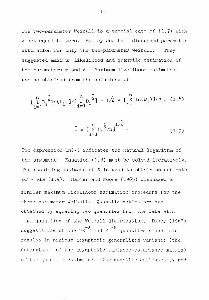
14
The two-parameter Weibull is a special case of (1.7) with
A set equal to zero. Bailey and Dell discussed parameter
estimation for only the two-parameter Weibull. They
suggested maximum likelihood and quantile estimation of
the parameters y and 6. Maximum likelihood estimates
can be obtained from the solutions of
n n 6 [ L D. 01n(D.)]/[ L Di] i=l l l i=l
l/a
n A 1/6 y = [ L D. 6 /n]
. 1 l i=
( 1. 8)
( 1. 9)
The expression ln(·) indicates the natural logarithm of
the argument. Equation (1.8) must be solved iteratively.
The resulting estimate of 6 is used to obtain an estimate
of y via (1.9). Harter and Moore (1965) discussed a
similar maximum likelihood estimation procedure for the
three-parameter Weibull. Quantile estimators are
obtained by equating two quantiles from the data with
two quantiles of the Weibull distribution. Dubey (1967) rd 4th . suggests use of the 93 and 2 quantiles since this
results in minimum asymptotic generalized variance (the
determinant of the asymptotic variance-covariance matrix)
of the quantile estimates. The quantile estimates (y and

15
o) are calculated from the 93rd quantile (Q93 ) and the th 24 quantile (Q 24 ) by applying
0 = ln{ln(0.07)/ln(0.76)}/ln(Q93/Q24)
-6 y = -ln(0.76)/(Q24 )
(1.10)
(1.11)
The shape parameter, o, is first estimated via (1.10) and
then the scale parameter, y, is estimated from (1.11) and
6 •
Once the parameters of the diameter distribution
have been estimated for specific sets of stand variables
from data sets, the estimates are compared with those
stand variables. Schnur (1934) presented the basic
technique after which modern efforts are modeled. Schnur
plotted parameter estimates against average stand diameter
at breast height and fitted smooth free-hand curves through
the data points. These curves could be used to predict the
parameters of the estimated diameter distribution from
average diameter. The modern approach consists of using
multiple regression techniques to predict the parameters
of the estimated diameter distribution from stand variables
by fitting a smooth curve to the data.
Recent efforts to estimate diameter distributions
consists of (1) collecting data consisting of measurement
16
of all tree diameters on a fractional part of an acre
(often 0.1-acre), and measurement of the stand variables
such as number of trees per acre, the average height of
the dominant and co-dominant trees (the largest trees),
and stand age, (2) repeating this process many times
(each sample is called a plot), (3) for each plot fitting
a smooth function such as the Weibull distribution to the
diameter data, thereby obtaining parameter estimates for
each set of stand variables, and (4) using multiple
regression techniques to estimate the diameter distribu-
tion parameters from the stand variables (one regression
equation is required for each diameter distribution
parameter). Once this process is complete, stand yield
is estimated from the estimated diameter distribution.
Bennett and Clutter (1968) first predicted yield
from estimated diameter distributions. They used the
beta distribution to describe the diameter distribution of
slash pine plantations, and to predict stand yields of
pulpwood, sawtimber, gum (used to make turpentine
and other products), and multiple-product yields
for mixtures of these products. An advantage of
this indirect yield estimation procedure is that it
is easily adapted to prediction of multiple-product
yield. Estimation of yield is accomplished by
(1) estimating the expected number of trees in each
diameter class (the range of diameters is divided into
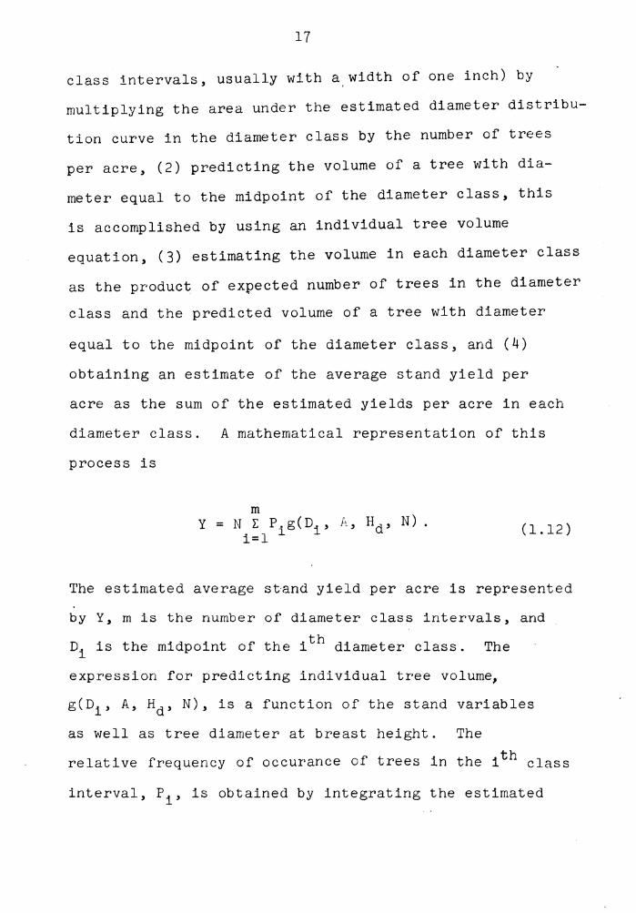
17
class intervals, usually with a width of one inch) by
multiplying the area under the estimated diameter distribu-
tion curve in the diameter class by the number of trees
per acre, (2) predicting the volume of a tree with dia-
meter equal to the midpoint of the diameter class, this
is accomplished by using an individual tree volume
equation, (3) estimating the volume in each diameter class
as the product of expected number of trees in the diameter
class and the predicted volume of a tree with diameter
equal to the midpoint of the diameter class, and (4)
obtaining an estimate of the average stand yield per
acre as the sum of the estimated yields per acre in each
diameter class. A mathematical representation of this
process is
m Y = N I: P. g (Di , f,, H d, N) •
i=l l (1.12)
The estimated average s~and yield per acre is represented
by Y, m is the number of diameter class intervals, and
Di is the midpoint of the ith diameter class. The
expression for predicting indi victual tree volume,
g(Di, A, Hd, N), is a function of the stand variables
as well as tree diameter at breast height. The
relative frequency of occurance of trees in the 1th class
interval, P1 , is obtained by integrating the estimated
18
diameter denstiy over the range of the ith diameter
class. This yield estimation procedure has been used
by Bennet and Clutter (1968) to predict yields of
slash pine plantations, and by Lenhart and Clutter
(1971), Lenhart (1972), and Smalley and Bailey (1974a)
to predict the yield of loblolly pine plantations.
Smalley and Bailey (1974b) used this technique to
predict the yield of shortleaf pine (Pinu~ eehinata)
plantations.
II. PROCEDURES
Data Collection
The data used for this study were from old-field
loblolly pine plantations> and from loblolly pine trees
grown free from competition. The study area, plot
selection procedures, and plot measurements were
described by Burkhart et al. (1972).
Study area. Data for this study were collected by
field crews from several industrial forestry organizations.
Selected loblolly pine plantations were sampled in the
Piedmont and Coastal Plain regions of Virginia, and in the
Coastal Plain region of Delaware, Maryland and North
Carolina. Data from 186 sample plots were used in
the analyses reported in this dissertation.
Flot selection. Temporary 0.1-acre, circular sample
plots were randomly located in selected stands. To be
sampled, plantations were required to be unthinned, contain
no interplanting, be free of severe insect or disease
damage, be unburned and unpruned, and be relatively free
of wildlings.
Plot measurements. On each 0.1-acre plot, dbh was
recorded to the nearest 0.1 inch for all trees in the
19

20
1-inch dbh class and above. Lach tree in the 8-inch
dbh class and above was classed as qualifying or not
qualifying for sawtimber. A sawtimber tree was defined
as being in the 8-inch dbh class or larger and having
at least one 16-foot sawlog to a 6-inch top diameter,
inside bark. Total height was recorded for at least one,
but usually two trees per 1-inch dbh class. Six to eight
dominant and co-dominaht trees were selected as site
sample trees and the total age of the stand was determined
from planting records, increment borings, or ring counts
at the stump of the felled specimens. th th On each plot two trees (the 10 and 20 trees
measured) were felled and cut into 4-foot sections for
detailed measurements. The following data were recorded
for each felled sample tree:
1. Diameter at breast height to the nearest
0.1 inch
2. Total tree height to the nearest 0.1 foot
3. Total age of the tree (age at the top of
each 4-foot bolt was also recorded for
dominants and codominants)
4. Diameters (inside and outside bark) at
the stump and at 4-foot intervals up the
stem to an approximate 2-inch tor:; diameter
(outside bark).
21
Additional data not described in Burkhart et al.
(1972) were collected for trees grown free of competition.
Eighty-one sample trees were located in Piedmont and
Coastal Plain Virginia. The trees were located in
abandoned fields, plantations, rights-of-way, and on
private lawns. They were chosen only if free of insect
damage and disease, fire damage, and any sign of competi-
tion as described by Krajicek et al. (1961). Measurements
made on each tree included:
1. Age from seed
2. Diameter at breast height to the
nearest 0.1 inch
3. Total tree height to the nearest
foot
4. Length of live tree crown to the
nearest foot
5. Two crown diameters, at the widest
crown expanse, measured perpendicular
to each other to the nearest foot.
Data were collected by the Chesapeake Corporation
of Virginia, Continental Can Company Incorporated,
Glatfelter Pulp Wood Company, Southern Johns-Manville
Products Corporation, and Union Camp Corporation. The
Virginia Division of Forestry contributed some open-grown
tree measurements.

22
Individual Tree Yield Equations
Individual tree yield equations were required to
estimate the yield of trees on each of the 186 sample
plots as a preliminary step to derivation and evaluation
of the yield estimation procedures. The same individual
tree equations were used as an integral part of the
indirect yield estimation procedures. The individual
tree yield equations used in this dissertation are
described by Burkhart et al. (1972) and are modifications
of the combined variable equation ( 1. 3); they were develop-
ed to simplify data collection. The total height data
(usually two trees per 1-inch dbh class) was used to
establish the relationship between dbh and total tree
height on each plot. The data on each plot were used to
estimate s2 , and s3 in
( 2. 1)
This equation was then used to predict total tree height
(H ) from tree diameter at breast height for each tree p
measured on the same plot. Individual tree volume was
then a function of tree diameter at breast height only,
described by
2 V = s0 + S1D Hp ( 2. 2)
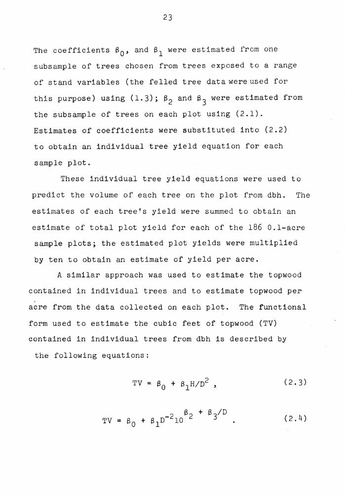
23
The coefficients s0 , and s1 were estimated from one
subsample of trees chosen from trees exposed to a range
of stand variables (the felled tree data were used for
this purpose) using (1.3); s2 and s3 were estimated from
the subsample of trees on each plot using (2.1).
Estimates of coefficients were substituted into (2.2)
to obtain an individual tree yield equation for each
sample plot.
These individual tree yield equations were used to
predict the volume of each tree on the plot from dbh. The
estimates of each tree's yield were summed to obtain an
estimate of total plot yield for each of the 186 0.1-acre
sample plots; the estimated plot yields were multiplied
by ten to obtain an estimate of yield per acre.
A similar approach was used to estimate the topwood
contained in individual trees and to estimate topwood per
acre from the data collected on each plot. The functional
form used to estimate the cubic feet of topwood (TV)
contained in individual trees from dbh is described by
the following equations:
( 2. 3)
TV (2.4)
24
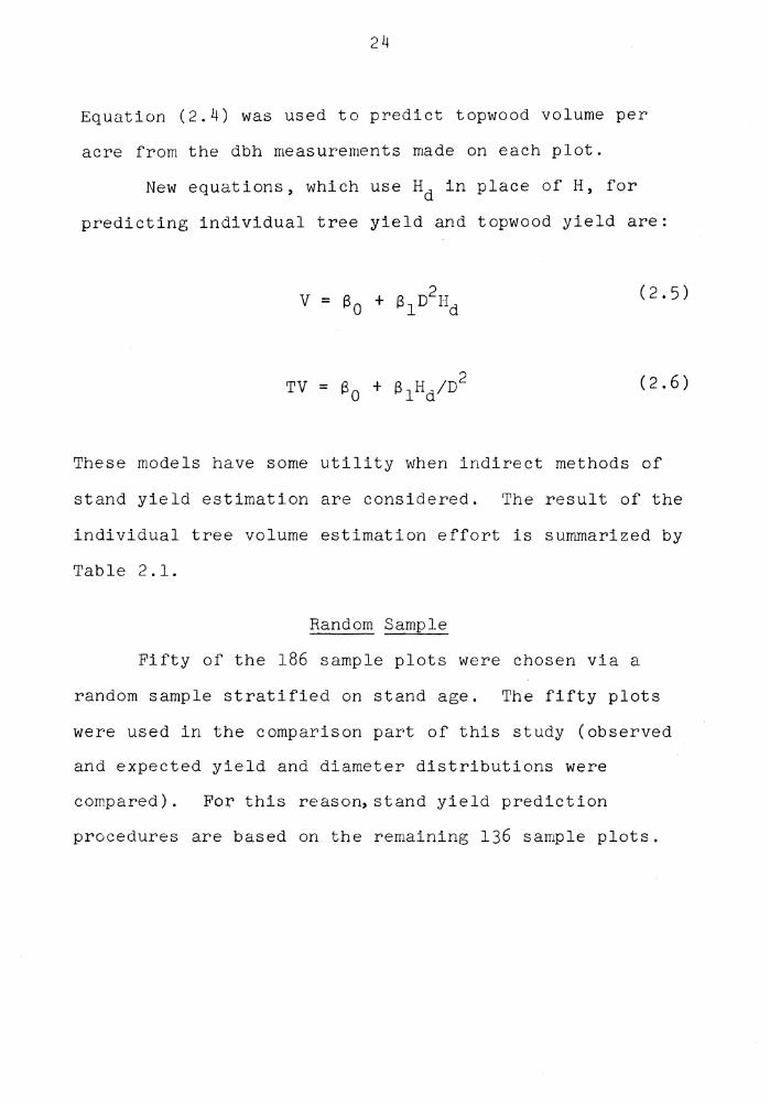
Equation (2.4) was used to predict topwood volume per
acre from the dbh measurements made on each plot.
New equations, which use Hd in place of H, for
predicting individual tree yield and topwood yield are:
( 2 . 5 )
TV (2.6)
These models have some utility when indirect methods of
stand yield estimation are considered. The result of the
individual tree volume estimation effort is summarized by
Table 2.1.
Random Sample
Fifty of the 186 sample plots were chosen via a
random sample stratified on stand age. The fifty plots
were used in the comparison part of this study (observed
and expected yield and diameter distributions were
compared). For this reason, stand yield prediction
procedures are based on the remaining 136 sample plots.

Table 2.1. Coefficients of individual tree volume equations
Coefficient Standard of Error of
Unit of Volume Measure Model Slope Intercept Determination Estimate
Cubic Feet 1. 3 0.11691 0.00185 0.970 0.495 Total Stem Inside Bark 2.5 -0.06136 0.00187 0.952 0.614
Cubic Feet Inside Bark 1. 3 -0.46236 0.00185 0.959 0.576 To 4 11 Top Outside Bark 2.5 -0.63594 0.00187 0.945 0.665
Board Feet 1. 3 * -23.67532 0.01102 0.517 0.002 International 0.25-inch 2.5 -37.23422 0.01332 0.856 12.738
Cubic Feet of Topwood 2.3 0.49318 2.7089 0.413 0.564 To 4" Top 2.6 0.67632 2.3883 0.427 0,557
* Weighted regression was used for this model. Least squares was used to estimate parameters in the model
2 2 V/D H = So/DH+ sl.
The model was solved for volume and used to estimate individual tree volume from D and H.
I\)
\.n
26
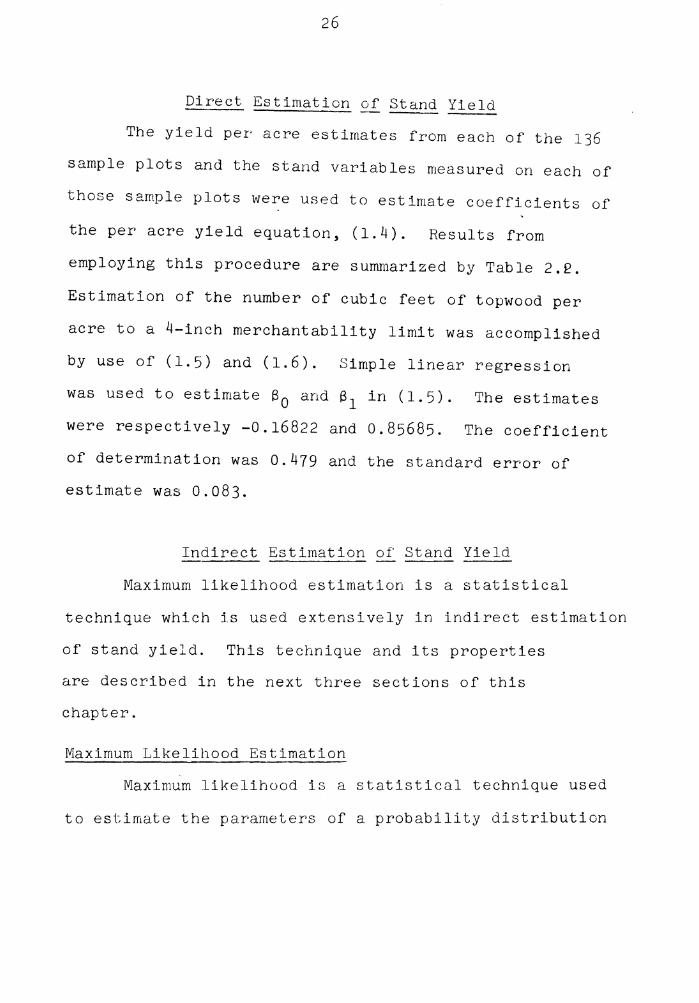
Direct Estimation of Stand Yield
The yield per acre estimates from each of the 136
sample plots and the stand variables measured on each of
those sample plots were used to estimate coefficients of
the per acre yield equation, (1.4). Results from
employing this procedure are summarized by Table 2.~.
Estimation of the number of cubic feet of topwood per
acre to a 4-inch merchantability limit was accomplished
by use of (1.5) and (1.6). Simple linear regression
was used to estimate B0 and B1 in (1.5). The estimates
were respectively -0.16822 and 0.85685. The coefficient
of determination was 0.479 and the standard error of
estimate was 0.083.
Indirect Estimation of Stand Yield
Maximum likelihood estimation is a statistical
technique which is used extensively in indirect estimation
of stand yield. This technique and its properties
are described in the next three sections of this
chapter.
Maximum Likelihood Estimation
Maximum likelihood is a statistical technique used
to estimate the parameters of a probability distribution

Table 2.2.Parameter estimates, coefficient of determination and standard error of estimate for per-acre yield prediction via the direct yield estimation-approach* for 136 sample plots in loblolly pine plantations
Unit of Measure of Volume
Cubic Feet Per Acre, Total Stem, Inside Bark
Cubic Feet Per Acre Inside Bark to a 4-inch Top (OB)
Board Feet Per Acre Interna-tional 0. 25-inch to a 6-inch Top (IB)
Coefficient of
Determination bo bl b2 b3 b4 (R2)
2.45498 -7.21875 0.32198 0.00819 0.00808 0.941
2.62827 -13.38634 0.45609 -0.01633 0.00571 0.934
4.88359 -68.40489 1.22336 -0.14121 .00921 0.812
* Model: Log10Y = b0 + b1 (1/A) + b2 (Hd/A) + b 3 (N/100) + b 4 (A)(Log10N)
Standard Error of Estimate s y·x
0.048
0.077
0.292
l\J -.J

28
from observations from that probability distribution.
This technique and properties of maximum likelihood
estimates are described in detail in chapter 5 of Zacks
(1971) and chapter 5 of Rao (1973). The method of maximum
likelihood is to find the parameter estimates which
maximize the likelihood function. The likelihood function
is defined as the joint probability density function or
probability mass function of the observations. Maximizing
this function with respect to choice of parameters results
in choosing the probability distribution with the largest
likelihood function for the data observed. A set of n
independent identically distributed random variables, {Xi}
each with probability density or mass function f(Xi' ~),
with parameter vector ~' have the following likelihood
function (L),
n L= Tif(X.,0).
i=l l -
"' The maximum likelihood estimates of 0, ~' are
( 2. 7)
obtained by maximizing L. A common technique is to maximize
ln(L). This results in the same estimates since the natural
logarithm is a monotonic transformation, and this often
simplifies the maximization problem. Classical optimiza-
tion techniques are commonly used, the partial derivative
29
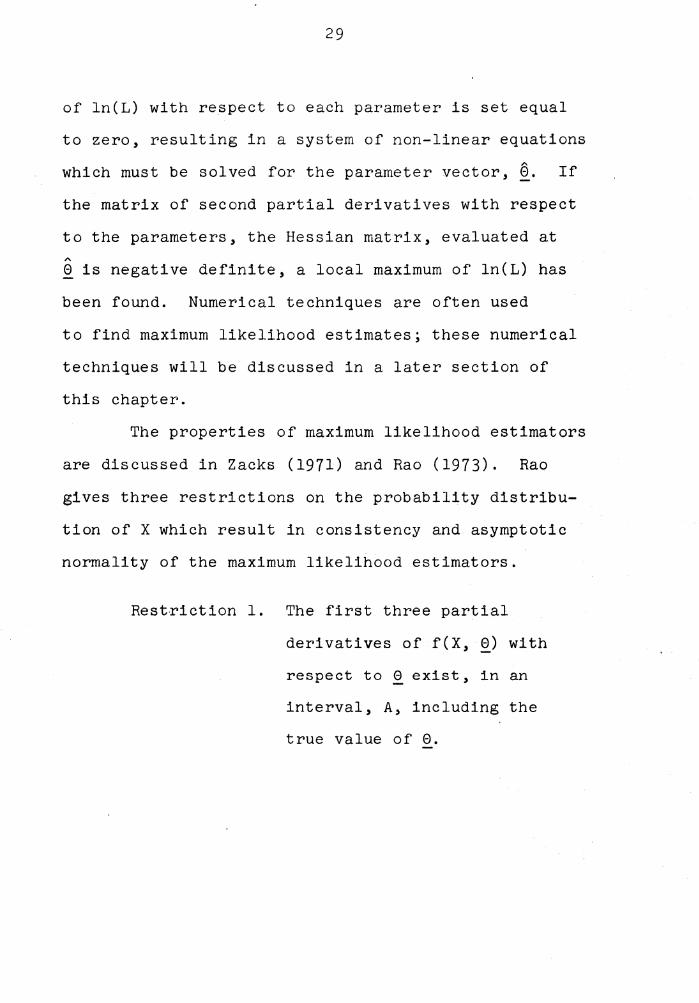
of ln(L) with respect to each parameter is set equal
to zero, resulting in a system of non-linear equations
which must be solved for the parameter vector, ~· If
the matrix of second partial derivatives with respect
to the parameters, the Hessian matrix, evaluated at A e is negative definite, a local maximum of ln(L) has
been found. Numerical techniques are often used
to find maximum likelihood estimates; these numerical
techniques will be discussed in a later section of
this chapter.
The properties of maximum likelihood estimators
are discussed in Zacks (1971) and Rao (1973). Rao
gives three restrictions on the probability distribu-
tion of X which result in consistency and asymptotic
normality of the maximum likelihood estimators.
Restriction 1. The first three partial
derivatives of f(X, 8) with
respect to 0 exist, in an
interval, A, including the
true value of e.
30
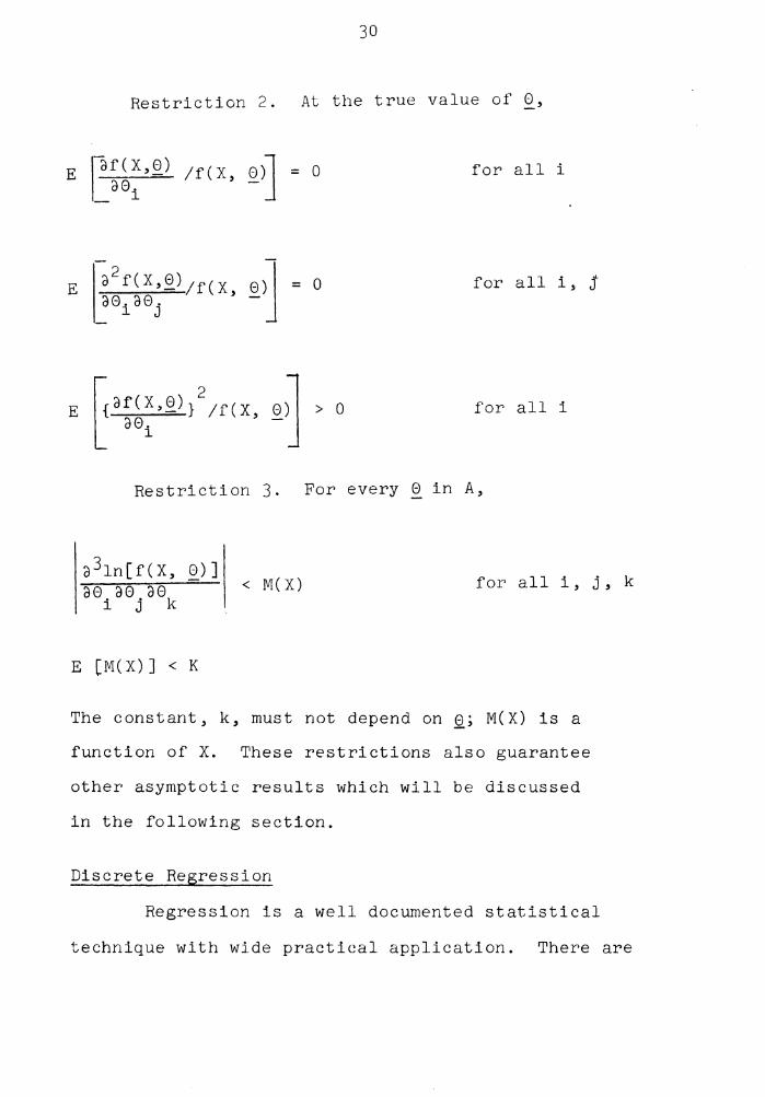
Restriction 2. At the true value of Q,
E af(X,Q) /f(X, Q)J = 0 ae. l
E a 2 f ( x ' ~) Ir ( x , e )-J = O ae.ae. l J
for all i
for all i, j
for all i
Restriction 3. For every 8 in A,
a31n[f(X, Q)] ae ae ae
i j k
E [M(X)] < K
< M(X) for all i, j, k
The constant, k, must not depend on Q; M(X) is a
function of X. These restrictions also guarantee
other asymptotic results which will be discussed
in the following section.
Discrete Regression
Regression is a well documented statistical
technique with wide practical application. There are
31
numerous references on regression analysis such as the
texts by Graybill (1961) and Draper and Smith (1966).
A basic assumption of most regression models is that the
dependent variable (y) is continuous. Numerous forest
management situations require modeling of discrete
random variables similar to Bernoulli trials. Some
examples of these forestry applications include mortality
of trees, presence or absence of a tree species, and
whether or not a tree is suitable for manufacture of
lumber. The topic of this section is the development of
a discrete regression model. The dependent variable will
be assumed to be a discrete random variable, similar in
nature to a Bernoulli trial. The exact probability mass
function assumed is described by
y = o, 1. (2.8)
The dependent variable, y, can assume the values zero and
one. Common situations where this model can be applied
are often described as success-failure, or life-death
settings. The probability of success or failure, or
life or death, is a function of a vector of independent
variables, !, and a vector of parameters, 8. No particular
functional form for g(!, Q) is assumed at this point; how-
ever, the function must be bounded between zero and one.

32
Reference to this model in the statistical
literature is directed to specific functional forms for
g(X, 8). Walker and Duncan (1967) and Hamilton (1974)
address the case where g(X, ~) is the logistic distri-
bution function and determine an iterative procedure
for finding least squares like estimates of e. Cox (1970)
also restricts discussion to the logistic function; he
discusses least squares and maximum likelihood estimation
of e. Probit analysis deals with the case where g(X, Q) is the normal or log-normal distribution function. Again
iterative procedures are used to determine least squares
estimates of the parameters. Garwood (1941) demonstrated
that the least squares and maximum likelihood estimates
are equivalent in probit analysis. Jennrich and Moore
(1975) discussed the use of standard least squares programs
in finding maximum likelihood estimates of e. The purpose of this section is to develop a general
theory concerning estimation of the parameters ~ and
inference on those parameters by using the general theory
of maximum likelihood. Maximum likelihood has intuitive
appeal that the least squares procedure lacks in this
instance. The least squares approach is to minimize the
sum of the squared distances from g(!, Q) to the data
points. The value of the dependent variable, y, must be
zero or one, hence least squares estimates minimize the

33
sum of the squared distances from g(!, Q) to zero or one.
Maximum likelihood estimates of 8 are derived from the
likelihood function for n observations of y and X, namely
n y 1-y L = TI [g(X., 8)] i[l - g(!i' 8)] i
i=l -l ( 2. 9)
A more convenient form is the lagarithm of the likelihood
function,
Maximization of ln(L) cannot be achieved using classical
techniques except for some elementary forms of g(X, Q). An iterative technique for maximizing ln(L) will be
introduced in the next section.
Inference on the parameter vector, Q, is described
in general in Chapter 6 of Rao (1973). The test of
hypothesis Q = ~ can be performed by using the likeli-
hood ratio statistic proposed by Neyman and Pearson (1928),
n ~)]yi[l 1-y.
n [g(X.' - g( x.' 8 )] l i=l -l -l ~
A = (2.11) n Q)]yi[l
1-y n [g(X.' - g( x.' Q) J i
i=l -l -l
The distribution of A under the null hypothesis can be
determined from (2.8) with 8 = ~' since A is a function
34
of the random variables {Y.} whose probability mass l
function is given by (2.6). Enumeration of all possible
permutations of the {Yi}, associated values of {!i}, ~'
and the probability of occurance of each permutation as
calculated from~.~ results in the exact distribution of
A. This information can be used to determine the
critical region of the test. The power of the test
can be determined for specific alternate values of 8
in a similar fashion.
The Neyman-Pearson likelihood ratio test can also
be used to test hypotheses of the form e = £(y); where
h is a vector of functions which depend on the vector of
parameters y. The number of elements in e is q, and
the number of elements in r. is S < q. Under the null
hypothesis the probability mass function of Y is given
by
y = o, 1. (2.12)
Under the null hypothesis, the likelihood function, L, is
given by
(2.13)
35
Maximum likelihood estimates of y can be found by applying
the same iterative scheme as is used to determine maximum
likelihood estimates of e. The maximum likelihood estimates
of y will be denoted i· The test statistic used to test the
hypotheses e = ~(y) is given by
(2.14)
An exact test cannot be performed since the true value of
e is not completely specified by the null hypothesis
(8 depends on y which is not given). An approximate test
can be performed by following a procedure similar to the
procedure used for the simple test of hypothesis. The
approximate distribution of {Y.} under the null hypothesis l
is given by
y = 0,1. (2.15)
This probability mass function, ( 2 .15 ), can be used in
place of (2.8) to determine the probability mass function
of A*. The critical region and power of the test for
specific alternative values of e are determined by
following the same procedure as in the simple test. If

36
the number of observations is large, corr~utational effort
to test the hypothesis may become prohibitively large.
In this case an asymptotic test can be used.
Rao (1973) demonstrated that the asymptotic
distribution of -2ln(A*) is chi-square with q-s degrees
of freedom under the null hypothesis if restrictions 1,
2, 3 listed in the previous section hold.
Restriction 1. This restriction is met if the
first three partial derivatives
of g(~, ~) with respect to 0 exist.
Restriction 2. For all values of 8,
E~P(y)/P(y~ = I aei , I
+ [g(x,0) JYc1-g(x,0) J-l-yG ag~X,Q) ag(X,Q) = o - -- ae. a0. l J

37
= [g(X,8)]-l[g(X,0)] + 0 - - - -
= 2 ~g(X,892 =I- 0 a0. '
l
if 0 < g(!, 8) < 1 and ag~~~SL) F= 0
Restriction 3. For every 8,
{ag(X,8) a0.
l
ag(X,0) a0.
J
a c x, 0) } {-1_-____ Y __ ~ a0k + [l-g(!,~)J2
38
2 {a g(X,8) a0.a0.
1 J
ag(X,8) a0 k
ag(X,0)} a0 i
which is bounded if O<g(X,0)<1 and the first three partial
derivatives of g(X,0) with respect to 0 are bounded. This
theory will be applied to forestry problems in later
sections of this chapter.
Optimization Theory
The purpose of this section is to describe general
procedures for optimizing functions. These procedures
will be used to determine maximum likelihood estimates
from data. Optimization schemes for functions of a
single variable and functions of more than one variable
will be discussed.
Optimization techniques found in the statistical
literature are based on the classical method of finding
the value of the variable or variables. for which the
derivative or partial derivatives vanish. These techniques
are outlined in Chapter 5 of Zacks (1971) and Chapter 5
of Rao (1973). The techniques described are based on
some modification of the Newton-Raphson method for solving
non-linear equations.
39
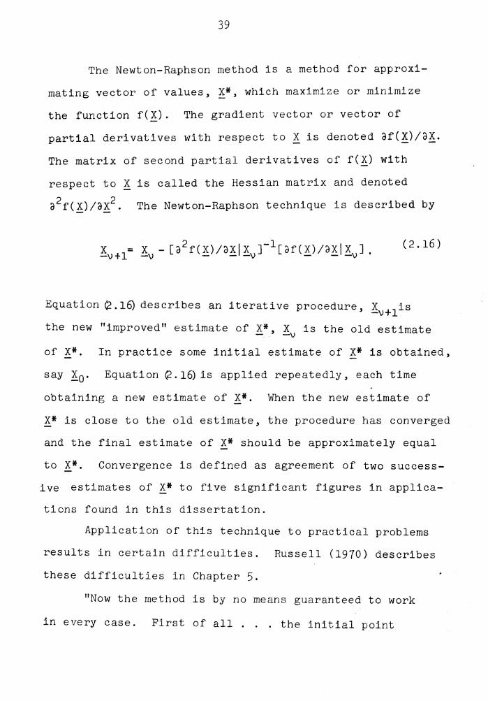
The Newton-Raphson method is a method for approxi-
mating vector of values, !*, which maximize or minimize
the function f(X). The gradient vector or vector of
partial derivatives with respect to X is denoted af(!)/3!.
The matrix of second partial derivatives of f(X) with
respect to X is called the Hessian matrix and denoted
a2r(X)/ax2 . The Newton-Raphson technique is described by
(2.16)
Equation ~-1~ describes an iterative procedure, X is -v+l the new "improved" estimate of X*, X is the old estimate - . -\)
of X*. In practice some initial estimate of X* is obtained,
say x0 . Equation ~.16) is applied repeatedly, each time
obtaining a new estimate of X*. When the new estimate of
X* is close to the old estimate, the procedure has converged
and the final estimate of X* should be approximately equal
to X*. Convergence is defined as agreement of two success-
ive estimates of X* to five significant figures in applica-
tions found in this dissertation.
Application of this technique to practical problems
results in certain difficulties. Russell (1970) describes
these difficulties in Chapter 5.
"Now the method is by no means guaranteed to work
in every case. First of all ... the initial point

40
!a should be fairly close to X*. Also,
Newton's method pays no attention to the fact that we
are looking for a minimum of f it is looking for a
point where 3f/3X = O. Such a point might or might not
be a minimum. It might be a maximum of f or a point where
of /ax = O but f has neither a maximum nor a minimum. In
fact, Newton's method for finding a maxima is exactly the
same as Newton's method for finding a minima."
In practice the Newton- Raphson technique works well
when optimizing f with respect to a single variable, but often
does not work well when ! represents a vector of variables.
A technique which does work well was suggested by
Davidon (1959). A refined version of this technique
is described in detail by Fletcher and Powell (1963).
They claim that "the method is probably the most powerful
general procedure for finding a local minimum which is
known at the present time." This technique is described
by
!v+l = !v - a H [af(X)/axJx J \) \) - - -\) ( 2 .17)
The positive scalar constant, is the number which
gives the greatest reduction in f. The matrix Hv is
updated at each iteration. Initially H1 is set equal to the
unit matri~ Thereafter it is updated according to
41
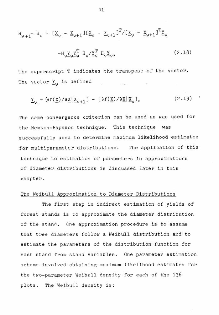
-H Y YT H /YT H Y v-v-v v -v v-v• (2.18)
The superscript T indicates the transpose of the vector.
The vector Y is defined -v
(2.19)
The same convergence criterion can be used as was used for
the Newton-Raphson technique. This technique was
successfully used to determine maximum likelihood estimates
for multiparameter distributions. The application of this
technique to estimation of parameters in approximations
of diameter distributions is discussed later in this
chapter.
The Weibull Approximation to Diameter Distributions
The first step in indirect estimation of yields of
forest stands is to approximate the diameter distribution
of the st2nrl. One approximation procedure is to assume
that tree diameters follow a Weibull distribution and to
estimate the parameters of the distribution function for
each stand from stand variables. One parameter estimation
scheme involved obtaining maximum likelihood estimates for
the two-parameter Weibull density for each of the 136
plots. The Weibull density is:

42
O<D, y, 6 (2.20)
The log-likelihood function associated with this probability
density function is
ln(L) n n 0
= nln(y) + nln(o) + (o-1) E ln(D.) - y E Di . i=l l i=l
(2.21)
The number of trees on a sample plot is n, and Di represents
the dbh of the ith tree on the plot. The two equations which
must be solved simultaneously to find maximum likelihood
estimates of y and o are
and
ln(L) ao
A " y,o
a1n(L) ay
n = + 7'
0
n = ~ = A A
y,o y
n E ln(Di)
i=l
n E
i=l
- A
y
D 0 = 0 1 '
n A
6 L: Di ln(Di) = 0. i=l
A
Equation (2.22) can be solved for y, resulting in
A n 6 y = n/ L: Di
i=l
A
(2.22)
(2.23)
(2.24)
This expression for y is then substituted into (2.23) to
obtain
n n/6 + Z ln(D.)
i=l l
43
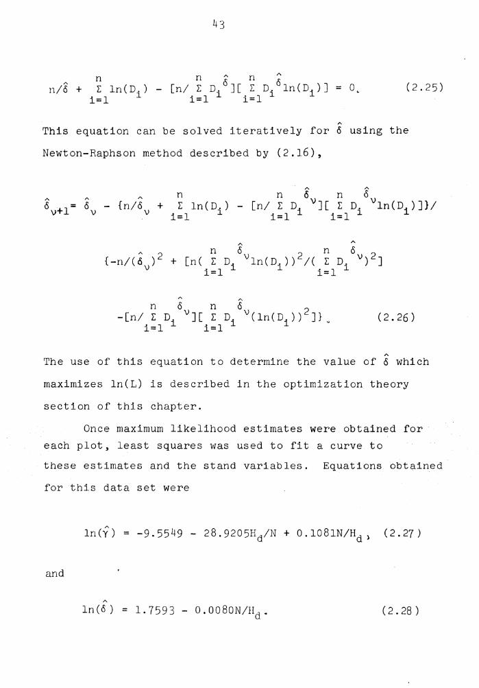
n A n "' 0 0 [n/ Z D. ][ Z D. ln(Di)] = 0, i=l l i=l l
(2.25)
"' This equation can be solved iteratively for o using the
Newton-Raphson method described by (2.16),
n n 6 n 6 ~v+l= ~v - {n/~v + Z ln(D.) - [n/ r Div][ Z D. vln(Di)]}/
i=l l i=l i=l l
A
n o n o {-n/ ( 6 ) 2 + [n ( Z Di v ln ( D. ) ) 2 I ( r D. v) 2 ]
\) i=l l i=l l
A A
n o n o -[n/ r Div][ r Di v(ln(D1 )) 2 J}
i=l i=l (2.26)
"' The use of this equation to determine the value of o which
maximizes ln(L) is described in the optimization theory
section of this chapter.
Once maximum likelihood estimates were obtained for each plot, least squares was used to fit a curve to
these estimates and the stand variables. Equations obtained
for this data set were
ln(y) = -9.5549 - 28.9205Hd/N + 0.1081N/Hd) (2.27)
and
A
ln(o) = 1.7593 - O.OOBON/Hd. ( 2. 28 )

44
Estimates of y and o must be positive according to (2.20).
Coefficients of determination are low (0.622 and 0.223,
respectively) as has been the case when this technique
has been applied in the past (e.g. Smalley and Bailey
1974a and 1974b). The standard errors of estimate were
1.559 and 0.158, respectively.
The coefficient of determination and the standard
error of estimate will be reported for each parameter
estimation model. The standard error of estimate is an
estimate of the standard deviation of observations about
the true regression line. A small standard error of
estimate indicates a good fit. The coefficient of
determination indicates the proportion of variation of
the independent variable about its mean which is explained
by the regression line. A coefficient of determination
close to one indicates a good fit. Comparison of the
standard error of estimate and coefficient of determina-
tion of different models is valid only when the dependent
variable of each model is the same. The coefficients of
determination and standard errors of estimate presented in
this dissertation are in general only indicators of the
goodness of fit of the model they describe and should not
be compared between models.
A second procedure for estimating y and o from th rd stand variables was based on the 24 and 93 quantiles.
45
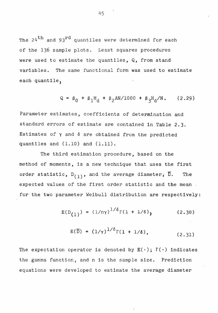
The 24th and 93rd quantiles were determined for each
of the 136 sample plots. Least squares procedures
were used to estimate the quantiles, Q, from stand
variables. The same functional form was used to estimate
each quantile>
(2.29)
Parameter estimates, coefficients of determination and
standard errors of estimate are contained in Table 2.3.
Estimates of y and o are obtained from the predicted
quantiles and (1.10) and (1.11).
The third estimation procedure, based on the
method of moments, is a new technique that uses the first
order statistic, D(l)' and the average diameter; D. The
expected values of the first order statistic and the mean
for the two parameter Weibull distribution are respectively:
l/o E(D(l)) = (l/ny) f(l + l/o), (2.30)
(2.31)
The expectation operator is denoted by E(·); f(·) indicates
the gamma function, and n is the sample size. Prediction
equations were developed to estimate the average diameter

Table 2. 3. Parameter estimates, coefficient'i of determination, and standard errors of estiIT.ate for prediction of quantiles 2nd minimum and average diameters on O .1- -acre plots in lob lolly pine stands
Coefficient Standard of Error of
Diameter to Be Determination Es tirra te Estimated bo bl b2 b3 R2 s y.x
24th Quantile 2.45759 0.05385 -0.05320 13.16225 0.838 0.469
93rd Quar..tile 3,96878 0.05484 -0.03535 30.41613 0.931 0.454
Minimum Diameter -0.05729 0.05294 -0.02001 14.7423 0.735 0.55~
Average Diameter 2.88209 0.05593 -0.04957 17.8446 0.932 0,336
.)::::'
°'
47
and the smallest diameter of the trees on the sample plots.
The same functional form as (2.29) was used to estimate
both average and smallest diameter from the stand
variables, namely
( 2. 32)
Parameter estimates, coefficients of determination and
standard errors of estimate are also contained in Table 2.3.
Estimates of y and o are obtained by equating the
estimated smallest tree diameter, D(l)' and E(D(l)), and
by equating the estimated average tree diameter, D)and
E(D). This resulted in a set of two simultaneous equations
in two unknowns,
D ( 1 ) = ( l/ny' ) 110 'r ( 1 + 1/ o' ) , (2.33)
and
o = (l/y 1 ) 116 'r<1 + l/o') (2.34)
These equations were solved simultaneously for y' and o'
0 ' = ln(n) (2.35) ln ( D') - ln(D(l)')
y' = ~(l ~.l/6')j 6 ' (2.36)
Estimates of y and cS for a specific set of stand variables
are obtained by first predicting D(l) and D from
prediction equations with the same functional form as
(2. 32). These estimates are used first to predict cS' from
D(l) and D via (2.35), and then to predict y' from 6' and
D via (2.36). The use of these diameter distribution
approximation procedures to indirectly estimate yields will
be discussed in a later section of this chapter.
The Normal Approximation to Basal Area Distributions
A new procedure for approximating the diameter
distribution of forest stands is to assume that the basal
areas (B) of trees in the stand are normally distributed.
This approach was inspired by examining frequency
histograms of basal area·s on the 136 sample plots. The
histograms for many of the plots appeared bell shaped,
hence it was conjectured that the normal distribution would
provide an accurate approximation to the frequency distribu-
tion of tree basal areas. The diameter distribution was
derived from the basal area distribution, since basal
area in square feet and diameter in inches are related
according to
( 2. 37)
This transformation was used to derive the diameter distri-
bution; the result is that if basal areas are normally
49
distributed, diameters are distributed as the square root
of a normal distribution.
The parameters (µ and cr 2 ) of the normal distribution,
f(B) = 1 '2 2 -(B-µ) /2a e co<B<co,
were estimated for each of the 136 sample plots. An
unbiased estimate of µ, B, was obtained from
n B = E Bi/n.
i=l
(2.38)
(2.39)
The basal area of the ith tree on the plot was Bi. An
unbiased estimate of a 2 was obtained from
s2 = n ;.... 2 E (Bi - B) /(n - 1).
i=l (2.40)
Once a parameter estimate was obtained for each
plot, least squares was used to fit a curve to the esti-
mates and the stand variables. Equations obtained for
this data set were
B = -0.17669 + 0.0054195 Hd + 101.56/N, (2.41)
and
S = 0. 042725 + 0. 0015267 AI-ld/;-"N. (2.42)

50
Coefficients of determination were 0.918 and 0.782,
respectively. The standard error of estimates were
respectively 0.0275 and 0.0185.
The procedure for approximating a diameter
distribution was to first estimate µ and a from stand
variables via (2.41) and (2.42). These estimates were
substituted into (2.38) to obtain an approximation of
the basal area distribution, from which transformation
(2.37) could be used to obtain an approximation to the
diameter distribution. This procedure was used in a
later section as part of an indirect yield estima-
tion scheme.
The Transformed Normal Approximation to Basal Area Distributions
Frequency historgrams from the 136 sample plots
seemed to indicate that some of the diameter distributions
were not normally distributed, but somewhat skewed. In
an attempt to introduce greater flexability into the
assumed basal area distribution, it was conjectured that
some power of basal area was normally distributed, namely
Bl-C/(1-C). This assumption results in a basal area
distribution described by
f (B) =
c " 1, -oo < B < oo. (2.43)
51
The parameters of this distribution are µ, 2 o , and C;
A represents stand age. Further justification for this
assumption will be presented in Chapter 4.
f C' µ' and 0 2 were Maximum likelihood estimates o ·
determined for each of the 136 sample plots. The likeli-
hood equation for this density function is:
n L = IT
i=l
B -C 1-C 2 2 2 i e-[Bi -Aµ(l-C)] /2Ao (1-C) r2lTA o
(2.44)
The log-likelihood function is more convenient to work
with;
n ln(L) = -C L ln(Bi) - (n/2)ln(2rrA) - (n/2)ln(o 2 )
i=l
(2.45)
The maximum likelihood estimates of C, µ, and o 2 are
obtained by taking the partial derivatives of ln(L) with
respect to each variable and equating each partial
derivative to zero. The resulting three equations are
solved simultaneously for C, µ, and o 2 \

A A Clln(L) ac = - ~ ln ( B. ) + { ( 1-C) ~ [B. l-C
i=l l i=l l Aµ(l-C)]
A
[B1 1-Cln(B1 ) - A~] - ~ [B 1 1-C-AC(l-C)J 2 }/[A~2 (1-C)3] 1=1
aln ( L) d]l
and
= 0)
= .~ ~i 1-c _ A~(1-c)J1~2 (1-c) = o, A A "'2 i=l L C,µ,a
(2.46)
(2.47)
a1n(L) aa 2
A') n ~ A A AJ2 "4 A 2 :;: -n/2a'- + L: B. l-·C - Aµ ( 1-C) /2Aa ( 1-C) l. =l l
r.. A A2 C,µ,a
= o. A
Equation (2.38) can be solved directly for µ,
" n l-C " µ = L: Bi /An(l-C).
1=1 "2 Equation (2.39) can be solved directly for a ,
~ 2 = . ~ ~i l-C - A~(l-C)J 2 /An(l-C) 2 • i=l l:
The value ofµ (2.49) can be substituted into (2.50),
"2 a = n A
L: (B.1-C i=l l
(2.48)
(2.49)
(2.50)
(2.51)
'"2 The value of µ from (2.49) and the value of a from (2.51)
53
can be substituted into (2.46) to obtain an expression
which contains only C,
A A
- ~ ln(B.) + {(1-C) ~ (B.l-C - s1/n)(B1 1-Cln(Bi) i=l l i=l l
A
- s1/n(l-C)) - ~ (B l-C - s1 /n) 2 }/ i=l i
A
n 1 c 2 A { ~ (B - - s1/n) (1-C)/n} = O. • 1 i i=...._
(2.52)
The expression s1 is defined by (2.56). This equation
must be solved iteratively for C. The Newton-Raphson
method described by (2.16) was used to accomplish this.
The expression on the left side of (2.52) corresonds to
af(X)/aX in (2.16). The iterative procedure used to find
C is described by
(2.53)
The expression on the left side of (2.52) evaluated at A A
Cv is equal to gv. The derivative of ·gv at Cv, is equal
tO g I• v I
The expressions gv and gv are described by
(2.54)
s2
S3 =
S4 =
s 5 =
and
=
54
~ B 1-C\) ' i=l i
n A
L: B 2-2C\J , i=l 1
A
n 1-C \) L: Bi ln(B1 )
i=l
;'\
n 2-2C \)
L: Bi ln(B1 ) i=l
" n 1-C \)
L: Bi ln(B.) 1=1 l
n L: ln(B1 )
i=l
(2.55)
(2.56)
(2.57)
(2.58) '
(2.59) '
(2.60) >
( 2. 61)
( 2. 6 2)

55
The algorithm defined by (2.53) through (2.62)
was used as described in the optimization theory section
of this chapter to compute maximum likelihood estimates
of C for each plot. Maximum likelihood estimates of µ
and cr 2 were computed for each plot using (2.49)
and ( 2. 50) .
Parameter estimates and measurement of stand
variables for each plot were used to develop equations to
estimate parameter values from stand variables. Equation
(2.63) was used t_o predict C,
C = 0.14198 + 0.66779AHdN/1000000. ( 2. 6 3)
Simple linear regression was used to estimate coefficients.
The coefficient of determination was 0.271 and the
standard error of estimate was 0.283. Equations (2.63) and
(2.64) were used jointly to estimate µ,
A(l-C)~ = -0.19332 + 0.043100A (2.64_1
The coefficient of determination was 0.400 and the standard .. error of estimate was 0.256. Equations (2.63) and (2.65) were
used jointly to estimate cr 2 ,
J A(l-C);2 = 0.013473A. (2.65)
The coefficient of determination was 0.325 and the standard
56
error of estimate was 0.107. The use of this method of
approximating basal area distributions and the resulting
approximate diameter distributions to indirectly estimate
yields of forest stands is described later in this chapter.
A Discrete Approximation to Diameter Distribution
A new approach to the estimation of the frequency
of occurance of tree diameters based on discrete regression
as described earlier in this Chapter is presented in this
section. Fundamental to this approach is the diameter
class interval system inherent to the measurement of tree
diameters at breast height. The roughness of tree bark
and irregularity of the shape (departure from circular)
of cross-sections of tree boles makes measurement of
tree diameters to closer than the nearest 0.1-inch
impractical. Measurement of tree diameters is tantamount
to grouping the trees into class intervals, each interval
0.1-inch in width. This situation is characteristic of
any measurement technique; the width of the class interval
is determined by the accuracy of the instruments used to
make measurements.
A system of class intervals referenced by the letter
j was used to describe the diameter classes. The first
diameter class which contained a tree observed on the
57-
136 sample plots was the 1. 2-inch diamete.r class. This
class includes diameters greater than 1.15 inches and
less than or equal to 1.25 inches. The last
diameter class was the diameter class of the tree with
the largest diameter on the 136 sample plots. This was
the 156th diameter class which included di~meters
greater than 16.65 inches and less than or equal to 16.75
inches.
The goal of this new prediction system is to
estimate the frequency of occurance of trees in each
diameter class from stand variables. This was accomplished
by estimating the probability that an observed tree falls
in the jth or larger diameter class from stand variables,
for all diameter classes which contained observations.
A model for such an estimation scheme can be based on the
Bernouli trial 1
(2.66)
The random variable Yijk·is equal to one if the kth
observed tree diameter on the ith plot is in the jth or
larger diameter class, and is equal to zero if the
diameter is in less than the jth class. The probability
Pij depends on j, the class interval which is being
58
referenced and on the stand variables (of the ith plot)
under which the tree was grown.
This probability might be functionally related to
statistics which describe the diameter distribution such
as the smallest tree diameter on the plot, D(l)' the
average tree diameter on the plot, Di, and sample quantiles,
Q. A sigmoid relationship between Pij and these statistics
seems reasonable. The sample average can be used to
illustrate this relationship. Pij represents the
probability that a tree is larger than some threshold
value, say t. When Di is much smaller than t a substantial
increase in Di should result in only a small relative
increase in Pij since the number of trees much larger
than Di should be small. When Di and t are not widely
separated, Pij and Di should be approximately linearly
related. When D. is much larger than t, nearly all the 1
trees are larger than t, therefore Pij is close to one
and again a substantial increase in Di results in only
a small increase in Pij" A model which incorporates
these concepts is the logistic distribution, which can
be written
1 a-D. . - 1
1 + e (2.67)

59
The constant a is positive. The functional form used to
describe the relationship between stand variables and
each of D(l)' D, and Qin (2.29) and (2.32) can be
substituted for Di in (2.67) to obtain
1
The coefficj_ents S j, s1 ., s2 ., and s3 . depend on the 0 J .,J J
(2.68)
jth class diameter. The stand variables on the ith plot
are represented by Ai; Ni, Ldi. Equations (2.66) and
(2.68) describe the probability mass function of Y1 j.
The likelihood function of Yij for a fixed value
of j is
136 n
i=l
136 n
1=1
ni yijk l-Yijk IT P.. (1-Pij)
k=l lJ (2.69)
The likelihood function can be written in a more convenient
form by considering the number of observations on the 1th
plot, n 1 and the number of those trees which are in the jth
or larger diameter class, m1j,
136 m n -m Lj = IT P ij(l-P ) i ij
i=l ij ij .. (2.70)
60
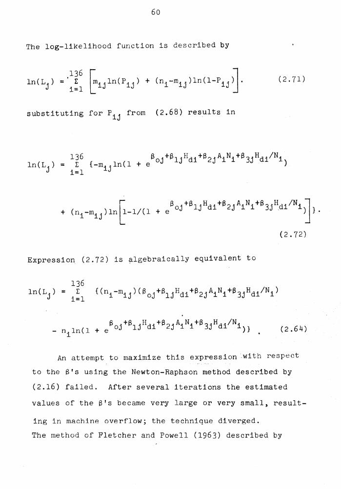
The log-likelihood function is described by
substituting for Pij from (2.68) results in
Expression (2.72) is ~lgebraically equivalent to
136 I:
i=l
(2.71)
(2.72)
(2.64)
An attempt to maximize this expression .with respect
to the S's using the Newton-Raphson method described by
(2.16) failed. After several iterations the estimated
values of the S's became very large or very small, result-
ing in machine overflow; the technique diverged.
The method of Fletcher and Powell (1963) described by
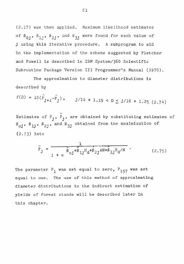
61
(2.17) was then applied. Maximum likelihood estimates
of Baj' Blj' s2j, and s3 j were found for each value of
j using this iterative procedure. A subprogram to aid
in the implementation of the scheme suggested by Fletcher
and Powell is described in IBM System/360 Scientific
Subroutine Package Version III Programmer's Manual (1970).
The approximation to diameter distributions is
described by
j/10 + 1.15 < D < j/10 + 1.2~ (2.74)
Estimates of Pj, Pj, are obtained by substituting estimates of
Soj' Slj' s2j' and s3 j obtained from the maximization of
(2.73) into
1 ·.o:---__,,,-----(2.75)
The parameter P1 was set equal to zero, P157 was set
equal to one. The use of this method of approximating
diameter distributions in the indirect estimation of
yields of forest stands will be described later in
this chapter.
62
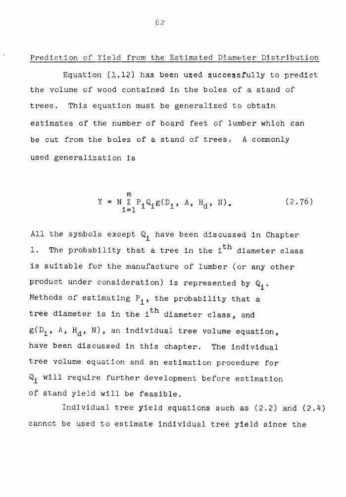
Prediction of Yield from the Estimated Diameter Distribution
Equation (l.lZ) has been used succe~~tully to predict
the volume of wood contained in the boles of a stand of
trees. This equation must be generalized to obtain
estimates of the number of board feet of lumber which can
be cut from the boles of a stand of trees. A commonly
used generalization is
(2.76)
All the symbols except Qi have been discussed in Chapter
1. The probability that a tree in the ith diameter class
is suitable for the manufacture of lumber (or any other
product under consideration) is represented by Qi.
Methods of estimating Pi' the probability that a
tree diameter is in the ith diameter class, and
g(D1 , A, Ha, N), an individual tree volume equation,
have been discussed in this chapter. The individual
tree volume equation and an estimation procedure for
Qi will require further development before estimation
of stand yield will be feasible.
Individual tree yield equations such as (2.2) and (2.4)
cannot be used to estimate individual tree yield since the
63
coefficients S2 and a3 in each equation were estimated for
a specific set of stand variables using the model described
by (2.1). An alternate method of individual tree yield
prediction is based on a tree height prediction equation
presented by Burkhart and Strub (1974),
loglOHp = 0.53815 + 0.77975 log1o<Hd) - 1.17713/A
+ 0.35468 log10 (N)/D + 4.11014/(AD) - 2.10285/D,
(2.77)
The coefficient of determination for this least squares
fit was 0.911 and the standard error of estimate was
0.040. The data set described earlier in this Chapter
was used to estimate coefficients. Estimates of tree
height, Hp' based on stand variables, A, Hd, and N, an~
tree diameter at breast height, D, can be substituted into
(1.3) and (2.3) to obtain the following individual tree
equations,
+0.35468 log10 (N)/D + 4~11014/(AD)-2.10285/D~
(2.78)
+0.35468 log10 (N)/D+4.11014/(AD)-2.10285/D).
(2.79)

64
Estimates of s0 and a1 are contained in Table 2.1. These
individual tree yield equations can be used in (2.76)
to predict stand yield. Alternatively, two new yield
equations, (2.5), and (2.6), developed earlier in this
chapter can be used. These new equations offer greater
simplicity, and are well suited to use in a new indirect
yield projection procedure that will be developed later
in this chapter.
The probabilities, Qi' were estimated from
individual tree data. When each tree diameter was
measured, the person conducting the inventory classified
the tree as suitable or not suitable for manufacture of
lumber. The estimates of Qi, Qi, were determined by
dividing the number of trees measured which fell in the
ith diameter class and were suitable for the manufacture
of lumber by the total number of trees measured which
fell in the 1th diameter class.
"' Diameter Class ( i ) Qi -
Less Than 8 0
8 0.3246
9 0.5322
10 0:9385
11 0.9851
Greater Tha.n 11 1
65
The class interval width used in the above estimation
procedure was one inch. The ith diameter class included
trees greater than i-0.45 inches, but less than or equal
to i+0.55 inches. This completes the information required
to estimate yield via (2.76). The results of a comparison
of yields estimated with (2.76) and other yield estimation
techniques is contained in Chapter 3.
A new class-interval-free approach to estimation
of yield from diameter distributions will be developed
from the procedure described by (2.76). A similar approach
has been published by Strub and Burkhart (1975). The class
interval system inherent in (2.76) is artificially
constructed with the class interval limits being arbitrarily
chosen. A class-interval-Yree system for yield prediction
can be obtained by examining the limiting form of (2.76) .as
the number of class intervals, m, increases without bound,
the width of individual class intervals approaches zero,
and the product of the number of class intervals and class
interval width remains constant. This procedure is
represented symbolically by
m Y = lim N L P.Q.g(D., A, Hd' N).
m~oo i=l l l l (2.80)
The probability Pi is obtained by integrating the
estimated diameter distribution, say f(D), over the .th range of the i diameter class. This is represented
symbolically by

66
D.+w/2 Pi = f 1 f(D)dD~
Di-w/2 (2.81)
The symbol w represents the width of a class interval.
Substituting this expression into (2.80) results in
Y = lim N (2.82) m+oo
The restriction that mw be constant dictates that m and
w are functionally related as described in
w = (U - L)/m. (2.83)
The symbol L represents the lower limit of the 1st class
interval and U represents the upper limit of the mth
class interval. Substituting this expression into (2.82)
results in
Y = lim N m+oo
It is now necessary to assume that Qi is a continuous
function of Di, say q(Di)'
(2.84)

Y = lim m+oo
m l:
i=l
67
D . + ( U-L) /(2 rrD l
J f(D)dDq(D 1 )g(Di,A,Hd,N) 0
D.-(U-L)/(2m) l
(2.85)
This assumption will be discussed later in this section.
The definition of the Riemann integral ensures that
(2.85) has the same limit as
m Y = lim N l: f(D. )liDiq(D1 )g(D. ,A,Hd;N) ..
. 1 l l i= ( 2. 86 )
m-+oo
The expression liDi is equal to the class interval width.
Another application of the definition of the Riemann
integral results in
u y N f f(D)q(D)g(D,A,Hd,N)dD.
L (2.87)
The estimation of stand yield in cubic feet of
solid wood in the tree boles when the Weibull approxima-
tion to diameter distributions is utilized will be used
as an example of the application of this new technique.
In this case q(D) = 1 for all values of D. Substitution
of (2.5) for g(D, A, Hd, N) and (2.20) for f(D) results in
00 0 Y = N fo(y~Do-le-yD ) 'a +a D2H )dD u ~..,o ..,1 ct 4 (2.88)
Analytical evaluation of the integral results in
68
( 2. 89 )
The appropriate estimates of a0 and B1 are listed in
Table 2.1. They are respectively -0.06136 and 0.00187.
Equations (2.27) and (2.28) or (1.10), (1.11) and (2.29)
or (2.32), (2.33) and (2.34) can be used to estimate y and
o. These estimates are substituted into (2.89). The
resulting value of Y is an indirect estimate of the
average yield per acre of the volume of solid wood
contained in the boles of trees in the stand.
When the trees in a stand are to be used for the
production of pulpwood, logs smaller than 4-inches in
diameter cannot be economically utilized.
Trees with a diameter at breast height smaller
than 4.55-inches cannot be economically utilized for
production of paper. Estimation of stand yield is
accomplished in this case by choosing an individual tree
volume equation which predicts cubic foot volume to a
4-inch merchantability limit, such equations are described
earlier in this chapter, (2.5) or (2.78), and coefficient
estimates are contained in Table 2.1. The function q(D)
takes on the following values '
q(D) =[: D < 4.55
D > 4.55 .. (2.90)

69
The diameter distribution, f(D), can be estimated via
one of the three schemes described earlier in this
Chapter. When all of these functions are substituted
irito (2.87), analytical evaluation of equation (2.87) was
The approximate value of the integral was not possible.
obtained in that case with the trapazoid rule. This
numerical technique is described by (2.82)
Juh(x)dx = i[h(L)+2h(L~W)+ ... +2h(U-W)+h(W)J. (2.91)
L
The symbol h(x) represents the function being integrated,
w is the class interval width. The class interval width
used in the numerical approximations found in this
dissertation is 0.01 inches. A smaller class interval
results in costly increases in computer time required to
calculate yield estimates, a larger class interval might
result in large errors due to the approximation.
A third indirect estimation procedure for predict-
ing board foot volume per acre (the average number of
board feet which can be cut from the boles of the trees
on an acre of land in a stand) was developed. The
individual tree volume equation~ (2.~ or ~.78),
were developed earlier in this chapter. They are also
summarized in Table 2.1. Any of the three diameter
distribution estimation procedures can be used. Choice

70
of a suitable functional forni for q(D) is more complex
than the previous two cases. Trees with a diameter at
breast height less than or equal to 7,55 inches are not
suitable for manufacture of lumber. The function q(D)
assumes the value zero over this range. Trees larger
than 7,55 inches may or may not be suitable for manufacture
of lumber. Plotting individual tree dbh versus relative
frequency of trees with the same dbh which were suitable
for manufacture of lumber indicates that an appropriate
choice for q(D) is
q(D) =~O l1 - e S(7.55-D)
D < 7.55 (2.92)
This continuous function of D is bounded between zero
and one. The function is monotone increasing and has
an upper asymptote of one. The derivative of q(D) is
defined for all values of D except D equal to 7,55. The
technique of discrete regression described earlier in
this chapter was used to estimate S. Data used to
estimate S were described earlier in this chapter
and consisted of the tree diameter at breast
height of each tree over 7,55 inches measured to the
nearest 0.1-inch plus an estimation of whether or not

71
the tree is suitable for production of lumber in the
opinion of the person measuring the tree.
The theory developed in the discrete regression
section of this chapter can be applied to the estimation
of f3 in
Y=O,l. (2.93)
The random variable Y assumes the value one if a tree D
inches in diameter is suitable for the manufacture of
lumber and Y assumes the value zero if the tree is not
suitable for the manufacture of lumber. This equation
was obtained by substituting the function describing q(D)
in (2.92) for g(X, ~) in (2.8). The log-likelihood
function can be obtained in a similar fashion from (2.10),
ln(L)= ~ Y.lnG - ef3(7. 55-Di)l + ~ (l-Yi)f3(7.55-D.). (2.94) i=l l L: J i=l l
The diameter of the ith tree measured is represented by
Di' Yi = 0 if the ith tree measured was not suitable for
manufacture of lumber and Yi = 1 if the .th tree was l
suitable for manufacture of lumber. An equation equivalent
to (2.94) which has greater computational efficiency is

ln(L)= ~ mJ.1nG j=l L
72
13(0.05-j/10) + r n.S(0.05-j/10),. (2.95) J .k
e j=l J
The symbol m. represents the number of trees between J
7.45 + j/10 and 7,55 + j/10 inches in diameter which
were suitable for production of sawtimber, nj represents
the number which were not suitable for production of
sawtimber, and k represents the number of diameter
classes observed. The Newton-Raphson method of optimiza-
tion can be used to find the value of 13 which maximizes
ln(L). This is the maximum likelihood estimate of 13 and
was found to be 1.2286 for the data collected on 186
sample plots.
It has been previously mentioned that data for
this study were contributed by several forest industries.
The personnel that gathered data, and therefore estimated
whether or not a tree is suitable for the production of
lumber, vary from company to company. It was hypothesized
that since personnel vary from company to company, perhaps
S also varies from company to company. The data collected
by Glatfelter Pulp Wood Company was divided into data
collected on the mainland and data collected on the eastern
shore of Maryland and Virginia, and treated separately.
The theory presented in the discrete regression section of
this chapter was used to test this hypothesis.
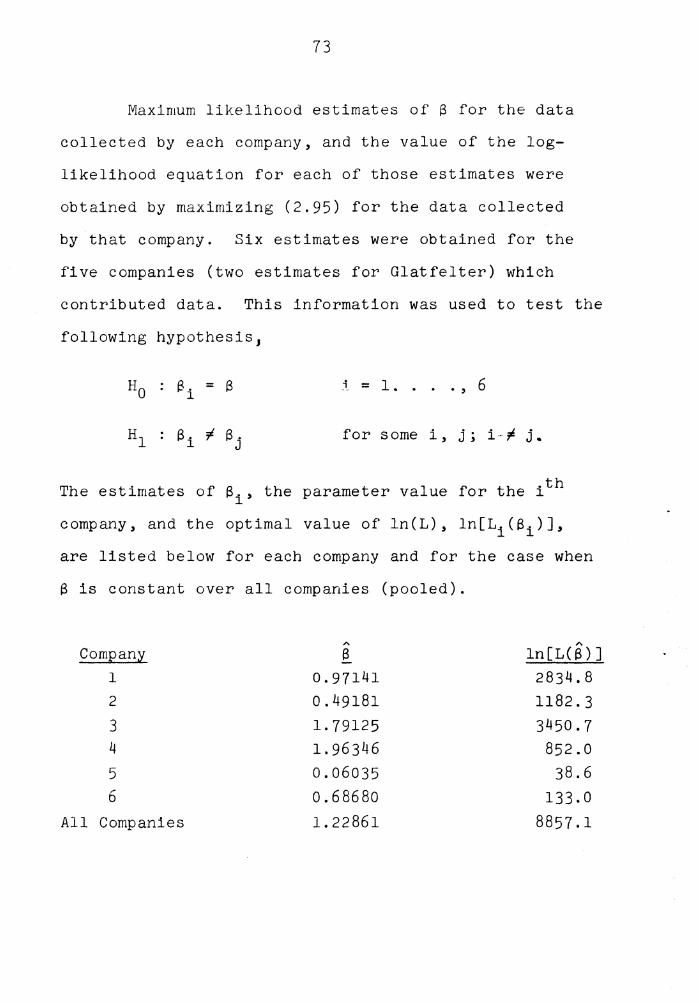
73
Maximum likelihood estimates of S for the data
collected by each company, and the value of the log-
likelihood equation for each of those estimates were
obtained by maximizing (2.95) for the data collected
by that company. Six estimates were obtained for the
five companies (two estimates for Glatfelter) which
contributed data. This information was used to test the
following hypothesis,
1\ = s i = 1 .... , 6
for some i , j ; i - ;t j.
The estimates of Si' the parameter value for the ith
company, and the optimal value of ln(L), ln[Li(Si)],
are listed below for each company and for the case when
Sis constant over all companies (pooled).
A A
Company s ln[L(S)] 1 0.97141 2834.8 2 0.49181 1182.3 3 1. 79125 3450.7 4 1.96346 852.0 5 0.06035 38.6 6 0.68680 133.0
All Companies 1. 22861 8857.1

74
The test statistic suggested, following (2.14), in the
discrete regression section of this chapter is
-2ln(A*)
A
= ln[L <a )J p p (2.96)
where ln[L.(S.)] indicates the maximum value of the log-1 l
likelihood function for the data from the ith company, A
and ln[Lp(Bp)] represents the maximum of the log-likelihood
function for the pooled data. Evaluation of (2.96)
resulted in a test statistic of 365.7.
A sample size of 2200 necessitates the use of an
asymptotic test. It has been demonstrated in the discrete
regression section that the asymptotic distribution of
the test statistic is chi-square with five degrees of
freedom. The hypothesis can be rejected at the 0.001
level of significance. For this reason a different
function, q(D) was used for prediction of board feet
yield for each company. The function used for each
company was (2.92) with a different estimate of
8 for each company.
After q(D) was determined board feet yields were
estimated via (2.87) and (2.93). In addition topwood
yield per acre was estimated. Topwood included wood
found between the 6-inch top diameter merchantability limit
for sawtimber and the 4-inch top diameter merchantability

75
limit for pulpwood plus wood found in trees not suitable
for the production of lumber. Each of the two components
of topwood was estimated separately. The component of topwood consisting of wood found
between the 6-inch merchantability limit for sawtimber
and the 4-inch merchantability limit for pulpwood was
estimated first. Individual tree volume equations of the
form (2.6) or (2.79) were used. Equation (2.92) was used to
estimate q(D), using a different value of S for yield
estimates for each company. Each .of the four diameter
distribution approximations were used. These functions
were substituted into (2.87) and final evaluation of
yield was accomplished via (2.91).
The second component of topwood yield was contained
in the trees which were not suitable for production of
lumber. Individual tree volume equations used to indirectly
estimate topwood yield were of the form of (2.5) and (2.78).
The proportion of the stand not suitable for production of
sawtimber can be estimated as one minus the proportion of
the stand which is suitable for sawtimber.

76
=f: D < 4.55
q(D) 4.55 < D < 7,55
lef3(7.55-D) D > 7,55 ( 2. 97)
The approximation to the diameter distribution can be any
one of the four developed earlier in this chapter.
Equations (2.86) and (2.91) were used to obtain estimates
of this component. The topwood yield estimate was the sum
of the estimates for each of the components. A comparison
of these indirect techniques for estimating topwood yield
and the direct method of estimating topwood yield is found
in chapter 3. This comparison is based on the 50 randomly
selected plots.
Comparison Techniques for Evaluating Yield Prediction
Kolmogorov-Smirnov Tests
Bailey (1972) suggested use of the Kolmogorov-
Smirnov test to check the validity of an assumed diameter
distribution. This test is described in chapter 4 of
Gibbons (1971). The test is used to compare the
empirical distribution function (in this case calculated
from the diameter measurements made on a plot) with some
hypothesized distribution function. The null hypothesis
tested is that the hypothesized distribution is the true
underlying probability distribution of the population

77
which was sampled. When applied to testing diameter
distributions the null hypothesis becomes the hypothesized
diameter distribution (such as the Weibull or the trans-
formed normal) is in fact the true diameter distribution.
One assumption of this test is that the hypothesized
distribution be completely specified, including specifica-
tion of all parameters. When Bailey applied this test,
he violated this assumption by estimating parameters of
the hypothesized diameter distribution (the Weibull)
from the data used to calculate the empirical distribu-
tion function. 'l'he violation of this assumption results
in an extremely conservative test, that is the probability
of a type I error is much less than specified.
Bailey used this procedure on 63 plots to perform
tests comparing two and three-parameter Weibull distribu-
tion to the observed diameter distribution. Several
estimation schemes including maximum likelihood were used
to estimate parameters of the hypothesized distribution
from the sample data. The proportion of the 63 plots on
which the null hypothesis was rejected was compared with
the probability of a type I error specified for all the
tests. If this proportion was less than the probability
of a type I error it was concluded that the null distribu-
tion was the correct approximation to the observed
78
diameter distribution. There is some danger in following
this procedure. It is known that in this case the test
is conservative, but the true probability of a type I
error is not known.
The danger of applying the Kolmogorov-Smirnov test
as Bailey suggests was examined via computer simulation.
Simulation techniques described by Box and Muller (1958)
were used to generate 1,000 samples, each containing 80
standard normal pseudo random numbers. Three different
methods were used to test the hypothesis: the variates
are normally distributed. The first test was the
Kolmogorov-Smirnov test described by Gibbons (1971),
for this test the hypothesized distribution was the
standard normal, that is a mean of zero and a variance of
one were specified. The second test was the test
suggested by Bailey (1972). The hypothesized distribution - 2 was the normal, however X and S were calculated from each
sample and used to estimate the mean and variance of each
of the 50 populations sampled. A third test suggested by
Stephens (1974) was applied to the same data. Stephens
presents modifications for the critical region of the
Kolmogorov-Smirnov test when the null hypothesis is that
the random variables are normally distributed, and the. - 2 population mean and variance are estimated by X and S .
Further discussion of the properties of this test was
presented by Green and Hegazy (1976).

79
The number of samples for which the null hypothesis
was rejected (hence it was concluded that the variates
were not normally distributed) was observed for each of
the three tests when the probability of a type I error
was 0.1, 0.05, and 0.01. The results of these tests are
listed in Table 2.4. If the test is operating correctly,
we would expect the proportion of samples for which the
null hypothesis was rejected to be approximately equal to
the probability of a type I error. Table 2.4 indicates
that the test suggested by Bailey is extremely conserva-
tive, and that the other two tests are not conservative.
The normal approximation to basal areas introduced
earlier in this chapter and described by (2.38) was used
to illustrate the danger of using the Kolmogorov-Smirnov
test as suggested by Bailey. The data collected on each
of the 186 sample plots were used to test the hypothesis:
tree basal areas are normally distributed. The mean and
variance of the basal areas was estimated for each plot
by X and s2 . The estimated mean and variance were used
to specify the null distribution. The results of the
tests suggested by Bailey and described in Table 2.5 seem
to indicate that basal areas are normally distributed
since the proportion of plots on which the null hypothesis
was rejected is less than the probability of a type I
error. However, as we have seen in the previous example,
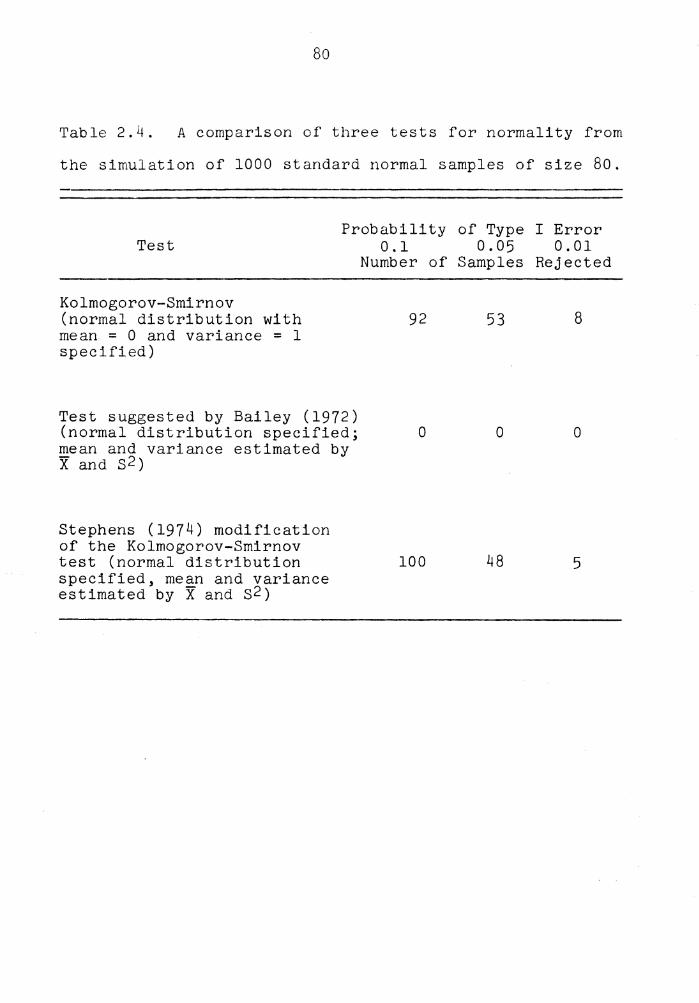
80
Table 2.4. A comparison of three tests for normality from
the simulation of 1000 standard normal samples of size 80.
Probability of Type I Error Test
Kolmogorov-Smirnov (normal distribution with mean = 0 and variance = 1 specified)
Test suggested by Bailey (1972) (normal distribution specified; mean and variance estimated by x and s2)
Stephens (1974) modification of the Kolmogorov-Smirnov test (normal distribution specified, mean and variance estimated by X and s2)
0.1 0.05 0.01 Number of Samples Rejected
92 53 8
0 0 0
100 48 5

Table 2.5. A comparison of tests for normality of tree basal areas on 186 sample plots from old-field loblolly pine plantations.
Test suggested by Bailey (1972 (normal distribution specified, mean and variance estimated by x and s2)
Stephens (1974) modification of the Kolrnogorov-Smirnov test (normal distribution specified, mean and variance estimated by x and s2)
Probability of a Type I Error 0.10 0.05 0.01
Number (and proportion) of Plots Rejectec
11(0.052) 5(0.027) 1(0.005)
52(0.280) 36(0.194) 20(0.108)
co I-'

82
the test described by Bailey is extremely conservative.
When Stephens' modification of the Kolmogorov-Smirnov
test was applied to the data it was concluded that
basal areas are not normally distributed. The results
of these tests, given in Table 2.5, are that the null
hypothesis was rejected on a larger proportion of the
plots than the probability of a type I error, hence the
conclusion that tree basal areas are not normally
distributed. The conservativeness of the test suggested
by Bailey resulted in an incorrect conclusion.
Stephens (1974) presents modifications of the
Kolmogorov-Srnirnov test for the cases of normal and
exponential null distributions. The modified tests are
not distribution-free since a new critical region must
be derived for each null distribution. Tests appropriate
for the Weibull distribution function, (2.20), the trans-
formed normal distribution function, (2.43), and the
discrete approximation described by (2.74) were not
available. A second problem encountered with the Stephens
modification of the Kolmogorov-Smirnov test is that this
procedure does not detect inaccuracy in prediction of
diameter distributions resulting from estimation of
parameters from stand variables. Such inaccuracy
effects the accuracy of approximations of diameter
distributions and yield estimates. A scheme
83
for making such a comparison between estimated and
observed diameter distributions should take into account
error introduced from estimation of parameters from
stand variables.
Such a comparison scheme is based on the 50 plots
removed at random from the total sample. The remaining
data, 136 plots, were used to develop schemes for estima-
ting parameters from stand variables. One of the diameter
distribution prediction schemes developed earlier in this
chapter can be used to estimate the diameter distribution
on each of the 50 randomly selected plots from stand
variables. In this manner the hypothesized diameter
distribution is completely specified for each plot without
using the tree diameter measurements from the 50 plots.
Observed and estimated diameter distributions were compared
via the Kolmogorov-Smirnov test in this manner. The results
of these tests indicate that perhaps none of the diameter
distribution schemes developed in this chapter are completely
adequate; these results are described in detail in the
following chapter.
Comparison of Observed and Estimated Yields
Each of the yield prediction techniques presented
in this chapter were implemented on the 136 sample plots
and the results were used to estimate the yield on the 50
randomly selected sample plots from the associated stand
84
variables. The average differences between observed and
expected yields as well as the variances of the differences
are presented in the next chapter.
Comparison of Culmination of Mean Annual Increment
The mean annual increment of a forest stand is the
yield per acre of the stand at a particular age divided
by that age. The point at which the mean annual increment
culminates (the age at which mean annual increment is
maximized) has been used as a criterion to determine
rotation length (the age at which the trees should be
harvested). Davis (1966, on pages 226 and 227) describes
the behavior of mean annual increment.
"Several items of significance hold in general regardless of the source and kind of data. The first is that on any given site the indicated rotation for maximum board foot production is longer than that for cubic foot production. This is because of the nature of the board foot unit; large trees contain pro-portionately more board feet than do small trees in comparison to cubic foot measure. Also, board foot measure does not contain all trees. only those above some specified minimum diameter limit. The second is that the rotation of maximum mean annual increment increases with decreasing site quality. As would be expected, this trend is much more strongly evident in board foot than in cubic foot growth. In addition to producing much less timber, the poorer sites take longer to reach their point of maximum mean annual increment."

85
Davis also indicates that loblolly pine stand
yield in cubic feet culminates between 30 and 35 years
whereas board foot yield culminates between 40 and 50
years. Davis does not indicate whether these ages are
for planted or natural stands. The age of culmination
of mean annual increment for a variety of stand variables
was calculated with each of the more promising yield
prediction techniques. These results are compared with
the notions described by Davis.
A direct and several indirect approaches to stand
yield estimation have been developed in this chapter. A
method for comparing the accuracy and precision of each
of the yield estimation techniques has been suggested.
The results of this comparison are described in chapter
3. A second criterion for comparing yield estimation
techniques is to examine the age of culmination of mean
annual increment for various combinations of stand
variables. The behavior of the age of culmination of
mean annual increment should behave in the manner described
by Davis (1966). The results of this comparison are
presented in chapter 3, A third method of comparison has
been suggested for the indirect yield estimation
techniques, which supply the forest manager with addition
information, namely an approximation to the frequency
distribution of tree diameters. A method for comparing

86
the accuracy of the diameter distribution approximations
has been developed in this chapter and the results of
this comparison are also presented in chapter 3.

III. RESULTS AND DISCUSSION
Kolmogorov-Smirnov Tests
Six diameter distribution estimation schemes were
presented in Chapter II. The first three diameter
distribution estimation schemes involved use of the
Weibull density density function, (2.20). The first
of these involved estimating the parameters of
the Weibull density function with (2.27) and (2.28). The
second technique involved estimating the 24th and 93rd
quantiles of the diameter distribution from stand variables,
and then estimating the parameters of the Weibull distribu-
tion function from the quantiles, (1.10) and (1.11). The
third scheme involved estimating the smallest and average
diameter from stand variables, and then estimating Weibull
parameters from (2.35) and (2.36). The fourth scheme
involved assuming that tree basal areas follow a normal
distribution, estimating parameters from stand variables
via (2.41), and (2.42), and obtaining the diameter
distribution from transformation (2.37). The fifth method
was to assume tree basal areas follow a transformed normal
distribution, estimate parameters from (2.63), (2.64), and
(2.65), and obtain the diameter distribution from trans-
formation (2.37). The last scheme was to estimate the
diameter distribution with the discrete approach described
by (2.74), and (2.75).
87

88
The six techniques were used to estimate the
diameter distribution on each of the 50 randomly selected
plots. Diameter measurements for the 50 plots were not
used in the estimation procedures. These estimated
diameter distributions were compared with the observed
diameter distributions by applying the Kolmogorov-Smirnov
test to the data on each of the 50 plots. The results of
this comparison are summarized in Table 3.1.
Examination of Table 3.1 indicates that among the
three Weibull schemes the estimators based on the smallest
and average tree diameters perform the worst. The other two
Weibull schemes are consistently better. No clear advantage
is evident in the two remaining Weibull schemes. The normal
approximation to basal area distributions performed as well
or better than any of the Weibull schemes. The transformed
normal approach is by far the worst of all the approximations
tested. Further discussion of this result will appear in
chapter 4. Performance of the discrete approximation to
diameter distributions was approximately the same as the
normal basal area approach. No one scheme exhibits a clear
advantage over all the other schemes. These tests also indi-
cate that perhaps none of the diameter distribution estima-
tion techniques considered thus far adequately describes
diameter distributions. An alternate method of estimating
diameter distributions will be developed in Chapter 4.
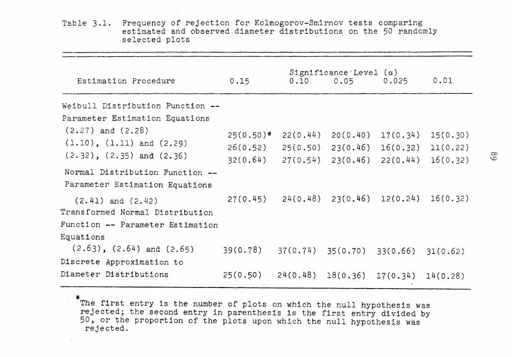
Table 3.1. Frequency of rejection for Kolmogorov-Smirnov tests comparing estimated and observed diameter distributions on the 50 randomly selected plots
Significance·Level (a) Estimation Procedure 0.15 0.10 0.05 0.025 0.01
Weibull Distribution Function Parameter Estimation Equations (2.27) and (2.28) 25(0.50)* 22(0.44) 20(0.40) 17(0.34) 15(0.30) (1.10), (1.11) and (2.29) 26(0.52) 25(0.50) 23(0.46) 16(0.32) 11(0.22) (2.32), (2.35) and (2.36) 32(0.64) 27(0.54) 23(0.46) 22(0.44) 16(0.32) Normal Distribution Function Parameter Estimation Equations
(2.41) and (2.42) 27(0.45) 24(0.48) 23(0.46) 12(0.24) 16(0.32) Transformed Normal Distribution Function -- Parameter Estimation Equations
(2.63), (2.64) and (2.65) 39(0.78) 37(0.74) 35(0.70) 33(0.66) 31(0.62) Discrete Approximation to Diameter Distributions 25(0.50) 24(0.48) 18(0.36) 17(0.34) 14(0.28)
* The first entry is the number of plots on which the null hypothesis was rejected; the second entry in parenthesis is the first entry divided by 50, or the proportion of the plots upon which the null hypothesis was rejected.
(X) \D

90
Comparison of Observed and Estimated Yield~
The direct and indirect yield prediction techniques
presented in chapter 2 were used to estimate yield from
stand variables on each of the 50 randomly selected plots.
The Weibull distribution functions and each of the three
associated parameter estimation schemes were used to
estimate yield. The transformed normal distribution
function and the discrete approximation to diameter
distributions were both used to estimate yield. Table
3.2 contains the results of this yield comparison.
The first row of Table 3.2 contains the comparison
of observed yields and yields estimated directly from
stand variables by use of multiple linear regression.
Equations (1.4) and (1.6) were used to obtain the yield
estimates. Estimates of coefficients in (1.4) are found
in Table 2.2. The estimates of a0 and a1 in (1.6) used in
yield estimation are, respectively, -0.16822 and 0.85685.
The next three rows of Table 3.2 contains a compari-
son based on the indirect method of yield estimation
utilizing the Weibull distribution and based on the class
interval method of yield estimation with 1-inch diameter
class intervals. The yield prediction procedure is
described by (2.76). Individual tree yield equations
(2.78) and (2.79) were substituted into (2.76). Each of
the three methods of parameter estimation was used to
obtain the three comparisons.
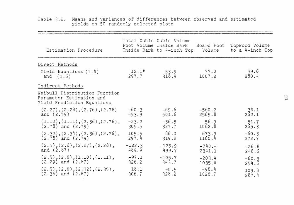
Table 3.2. Means and variances of differences between observed and estimated yields on 50 randomly selected plots
---··---------------Total Cubic Cubic Volume Foot Volume Inside Bark Board Foot Topwood Volume
Estimation Procedure Inside Bark to 4-inch Top Volume to a 4-inch Top -------·-------------Direct Methods Yield Equations (1.4)
and ( 1. 6)
Indirect Methods Weibull Distribution Function Parameter Estimation and Yield Prediction Equations
12.1* 297,7
(2.27),(2.28),(2.76),(2.78) -60.3 and (2.79) 493,9 (1.10) ,(1.11) ,(2.36) ,(2.76)' -23.2 (2.78) and (2.79) 305.5 ( 2 . 32) ' ( 2 . 3 4) ' ( 2. 36) ' ( 2 . 7 6) ' 10 5 . 5 (2.78) and (2.79) 297.4 (2.5),(2.6),(2.27),(2.28), -122.3 and (2.87) 489.9 (2.5),(2.6),(1.10),(1.ll), -97.1 (2.29) and (2.87) 326.2 (2.5),(2.6),(2.32),(2.35), 18.1 (2.36) and (2.87) 306.7
53,9 318.9
-69.6 501. 6 -36.5 327.7 86.o
319.2 -125.9
499,7 -105,7 343,7 -0.5
328.2
77,0 1007.2
-560.2 2565.8
56.9 1062.8
673.9 1160.4 -740.4 2341.1 -203.4 1035.4
498.4 1026.7
39.6 280.4
34.1 262.1 -51. 7 265.3 -60.3 272.7 -26.8 248.6 -60.3 254.6 109.8 287.4
\0 I-'

Table 3.2 (Cont)
Estimation Procedure
Total Cubic Cubic Volume Foot Volume Inside Bark Inside Bark to 4-inch Top
Board Foot Topwood Volume Volume to a 4-inch Top
Normal Distribution Function Parameter Estimation and Yield Prediction Equations (2.5),(2.6),(2.41),(2.42), and (2.87)
Transformed Normal Distribution Function -- Parameter Estimation and Yield Prediction Equations (2.5),(2.6),(2.63),(2.64), (2.65) and (2.87) Discrete Approximation to Diameter Distributions Parameter Estimation and Yield Prediction Equations (2.76),(2.78) and (2.79) (0.1-inch class intervals) (2.78),(2.79) and (2.87)
*
-67.3 382.4
-953.9 1038.4
-27.0 306.4
-27.0 306.4
-98.3 395,9
-1016.4 1018.6
-32.4 324.6
-32.4 324.6
-42.6 1046.3
-6575.8 6281.8
-66.3 1126.7 -60.0
1106.6
The first entry is the average difference (observed plot yield minus estimated plot yield); the second estimate is the variance of the differences.
-87.8 307.5
348.1 517.0
-14.5 249,5 -14.2 234.7
\D I\)

93
The fifth through seventh rows of Table 3.2 are
based on estimates calculated from the Weibull distribu-
tion function and the class-interval-free approach to
yield estimation. The yield prediction procedure is
described by (2.87). Individual tree yield equations
(2.5) and (2.6) were substituted into (2.87). Again
each of the three methods of parameter estimation was
used to obtain the three comparisons.
The normal basal area approach was used to
estimate yields described in row eight of Table 3.2.
Parameters were estimated from (2.41) and (2.~2), then
substituted into (2.38). The estimated diameter
distribution was derived from this estimated basal area
distribution, (2.38), and transformation (2.37). The
estimated diameter distribution and individual tree
volume equations (2.5), and (2.6) were substituted into
(2.87) to obtain indirect yield estimates.
The ninth row of Table 3.2 contains a comparison
based on the transformed normal distribution function
and the class-interval-free approach to yield prediction.
Yield esti~ation equation (2.87) and individual tree yield
equations (2.5) and (2.6) were used to calculate yield
estimates.
The last two rows of Table 3.2 contain a comparison
based on the discrete approximation to diameter

94
distributions. The comparison contained in the tenth
row is based on the class interval approach to yield
prediction. The class interval width used in estimation
was 1/10-inch. Equation (2.76) describes the procedure
used. Individual tree volume equations (2.78) and (2.79)
were substituted into (2.76). The average number of
trees suitable for production of lumber by diameter
class on the 186 sample plots was substituted for Qi.
The 11th row of Table 3.2 is a comparison based on the
class-interval-free method of yield prediction. This
procedure is described by equation (2.87). Individual
tree yield equations (2.78) and (2.79) were used. The
only difference between yield estimates used in rows nine
and ten is the method of estimating the probability that
a tree is suitable for production of lumber. Equation
(2.92) was used in row ten. A comparison of rows nine
and ten indicates that (2.92) is preferred over class
averages for estimating the pfobability that a tree is
suitable for production of lumber from tree dbh.
The direct method of yield estimation performed
nearly as well as any of the indirect yield estimation
techniques for estimation of all products considered. The
Weibull distribution function, quantile estimation of
parameters, and the class interval yield estimation
procedure with one inch class intervals was also
95
quite accurate in predicting total cubic foot volume
and cubic foot volume to a 4-inch top. The normal basal
area approach provided accurate and precise estimates
of board foot yield, however, total cubic volume,
and cubic volume to a 4-inch top estimates were less
accurate, and topwood volume estimates were not nearly
as accurate as estimates obtained via direct estimation
of topwood yield. The discrete diameter distribution
approach provided accurate yield estimates of all
products. The transformed normal distribution proved
a poor choice for estimating yield of loblolly pine stands.
Comparison of Age of Culmination of Mean Annual Increment
Four of the most accurate (as determined in the
previous section) yield estimation procedures were
compared. The first estimation procedure was the direct
method of estimating yield from stand variables,
described by (1.4). The second and third estimation
procedures were indirect techniques based on the Weibull
distribution function. The second procedure made use of
quantile parameter estimates, from equations (1.10), (1.11),
and ( 2 .·29 ), and the !-inch-class-interval method of yield
estimation. The third technique made use of parameter
estimates based on the smallest and largest diameters,

96
from equations (2.32), (2.35), and (2.36), and the class
interval-free method of yield estimation. All of
these yield estimation procedures appear in the compari
son described by Table 3.1.
Each of these yield estimation methods requires
input of the stand variables age (A), average height of
the dominant and codominant stand (Hd), and existing
number of trees per acre (N). Yield at various ages
must be calculated to determine the age at which mean
annual increment culminates, hence Hd and N must also be
estimated for each age for which a yield estimate is
calculated. Estimation of Hd is accomplished by assuming
a site index (S) and then using site index curves to
estimate Hd from A. Estimation of N is accomplished by
assuming an initial number of trees per acre at age
zero (N0 ) and then using survival curves to estimate N
from A.
The site index curves used in this part of the
study were developed by Burkhart et al. (1972). They
can be used to estimate Hd from A and S,
Hd = S(l0)0.23461 - 5.86537/A (3.1)
Site index, S, is a measure of the growing quality of
the land upon which the trees are planted, in particular
97
s is the aver·age height of the dominant and codominant
trees at age 25.
The survival curves used in this study were developed
by Lenhart and Clutter (1971). These survival curves are
The symbol¢(·) represents the standard normal distribu-
tion function. The results of the comparison of the age of
culmination of mean annual increment for the different
yield estimation techniques appear in Tables 3.3, 3.4, 3.5,
3.6, and 3. i None of the yield estimation systems behaves
exactly as described by Davis (1966).
The direct method of yield estimation of cubic
foot yield does not culminate before age 50 on poor
sites. Culmination is early on the better sites. The
board foot volumes culminate too early on all sites. The
relationship between site index and age of culmination
of mean annual increment is monotone decreasing as
described by Davis.
The indirect method utilizing the Weibull distribu-
tion function, quantile estimators, and 1-inch class
intervals culminated at approximately the correct age
for cubic foot and board foot yield. This method does

98
Table 3.3. Age at which mean annual increment culminates for various site index and initial density combinations when yields are estimated directly from stand variables via multiple regression equation (1.4).
Site Index 600
Initial Number of Trees Per Acre 800 1000 1200
Cubic Volume to a Four-Inch Top 40 50+(72.3)* 50+(74.7) 50+(76.1) 50+(76.8) 50 50+(94.9) 50+(98.l) 50+(99.9) 50+(100.9) 60 25(124.0) 26(123.1) 50+(131.2) 50+(132.4) 70 20(190.5) 23(187.8) 23(184.5) 23(180.8) 80 90
40 50 60 70 80 90
*
20(297.2) 19(468.2)
36(22.3) 32(56.9) 29(155.3) 26(446.9) 25(1336.9) 23(4123.1)
21(292.4) 20(459.7)
21(286.4) 20(449.6)
Board Foot Volume 37(15.3) 32(38.7) 29(105.0) 27(300.4) 25(895.4) 24(2746.8)
38(10.8) 33(27.2) 29(73.2) 27(208.3) 25(617.8) 24(1889.7)
21(279.9) 20(438.8)
39(7.9) 33(19.6) 30(52.4) 27(148.0) 25(436.5) 24(1331.2)
The first entry is the age at which mean annual increment culminates, the second entry is the mean annual increment at this age. An entry of 50+ indicates that mean annual increment culminates after age 50, in this case the second entry is the annual increment at age 50.
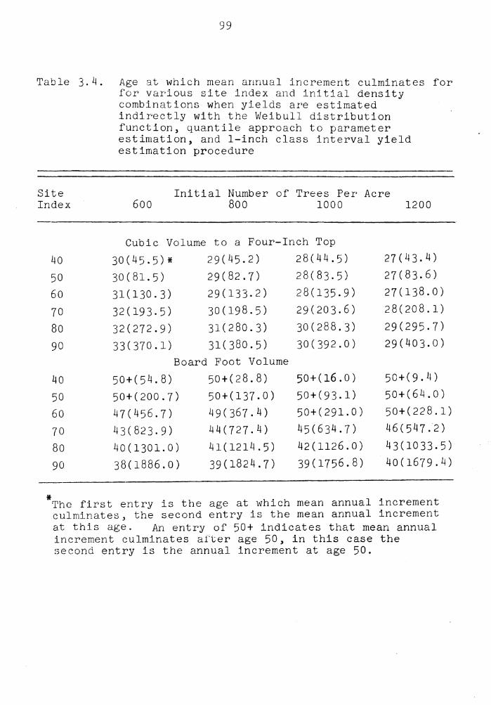
99
Table 3.4. Age at which mean annual increment culminates for for various site index and initial density combinations when yields are estimated
Site Index
40 50 60 70 80 90
40 50 60 70 80 90
indirectly with the Weibull distribution function, quantile approach to parameter estimation, and 1-inch class interval yield estimation procedure
Initial Number of Trees Per Acre 600 800 1000 1200
Cubic Volume to a Four-Inch Top
30(45.5)* 29(45.2) 28(44.5) 27(43.4)
30(81.5) 29(82.7) 28(83.5) 27(83.6)
31(130.3) 29(133.2) 28(135.9) 27(138.0)
32(193.5) 30(198.5) 29(203.6) 28(208.1)
32(272.9) 31(280.3) 30(288.3) 29(295.7)
33(370.1) 31(380.5) 30(392.0) 29(403.0) Board Foot Volume
50+(54.8) 50+(28.8) 50+(16.0) 50+(9.4)
50+(200.7) 50+(137.0) 50+(93.1) 50+(64.0)
47(456.7) 49(367.4) 50+(291.0) 50+(228.1)
43(823.9) 44(727.4) 45(634.7) 46(547.2)
40(1301.0) 41(1214.5) 42(1126.0) 43(1033.5)
38(1886.0) 39(1824.7) 39(1756.8) 40(1679.4)
* The first entry is the age at which mean annual increment culminates, the second entry is the mean annual increment at this age. An entry of 50+ indicates that mean annual increment culminates after age 50, in this case the second entry is the annual increment at age 50.
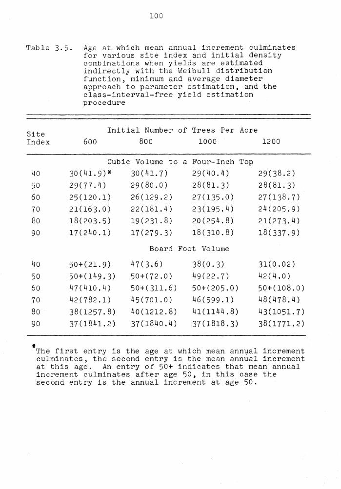
100
Table 3.5. Age at which mean annual increment culminates for various site index and initial density combinations when yields are estimated indirectly with the Weibull distribution function, minimum and average diameter approach to parameter estimation, and the class-interval-free yield estimation procedure
Site Index
40 50 60 70 80 90
40 50 60 70 80 90
*
Initial Number of Trees Per Acre 600 800 1000
Cubic Volume to a Four-Inch Top 30 ( 41. 9) * 29(77.4) 25(120.1) 21(163.0) 18(203.5) 17(240.1)
50+(21.9) 50+(149.3) 47(410.4) 42(782.1) 38(1257.8) 37(1841.2)
30(41. 7) 29(80.0) 26(129.2) 22(181.4) 19(231.8) 17(279.3)
29(40.4) 28(81.3) 27(135.0) 23(195.4) 20(254.8) 18(310.8)
Board Foot Volume
47(3.6) 50+(72.0) 50+(311.6) 45(701.0) 40(1212.8) 37(1840.4)
38(0.3) 49(22.7) 50+(205.0) 46(599.1) 41(1144.8) 37(1818.3)
1200
29(38.2) 28(81. 3) 27(138.7) 24(205.9) 21(273.4) 18(337.9)
31(0.02) 42(4.0) 50+(108.0) 48(478.4) 43(1051.7) 38(1771.2)
The first entry is the age at which mean ann~al increment culminates, the second entry is the mean annual increment at this age. An entry of 50+ indicates that mean annual increment culminates after age 50, in this case the second entry is the annual increment at age 50.

101
Table 3.6. Age at which mean annual increment culminates for various site index and initial density combinations when yields are estimated indirectly with the normal basal areas approach to diameter distribution estimation and the class-interval-free yield estimation procedure
Site Index 600
Initial Number of Trees Per Acre 800 1000 1200
Cubic Volume to a Four-Inch Top 40 30(54.9) 33(56.2) 36(57,9) 38(59.8) 50 60 70 80 90
40 50 60 ·70 80 90
*
28(88.2) 27(128.8) 26(176.4) 26(230.9) 25(292.5)
50+(125.9) 50+(261.8) 48(438,3) 41(663.0) 37(939.6) 34(1266.5)
30(94.18) 28(141.5) 27(197.9) 27(263.3) 26(337.5)
32(100.1) 29(153.6) 28(218.2) 27(293.6) 27(379.5)
Board Foot Volume
50+(113.6) 50+(261.4) 50+(462.8)
·45(716.7) 39(1036.1) 36(1421.2)
50+(104.2) 50+(260.8) 50+(483.8) 47(767.1) 41(1125.4) 37(1564.1)
33(105.8) 30(165.1) 29(237.3) 28(322.0) 27(419.0)
50+(96.7) 50+(260.2) 50+(502.0) 49(813.7) 42(1208.0) 38(1696.4)
The first entry is the age at which mean annual increment ~ulminates, the second entry is the mean annual increment at this age. An entry of 50+ indicates that the mean annual increment culminates after age 50, in this case the second entry is the annual increment at age 50.
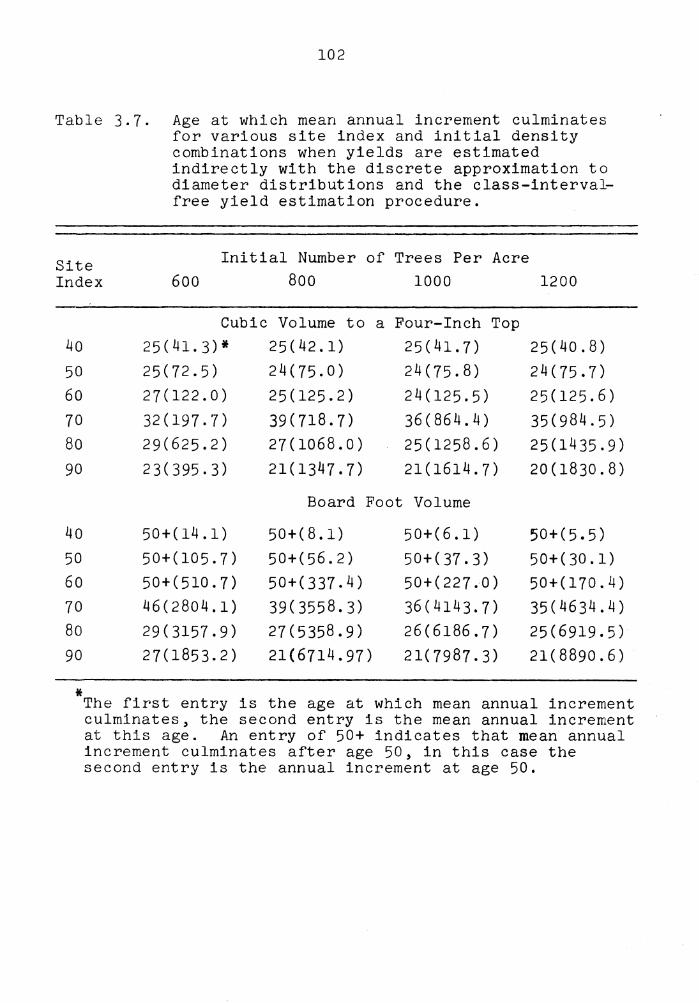
102
Table 3.7. Age at which mean annual increment culminates for various site index and initial density combinations when yields are estimated indirectly with the discrete approximation to diameter distributions and the class-interval-free yield estimation procedure.
Site Index
Initial Number of Trees Per Acre 600 800 1000 1200
40 50 60 70 80 90
40 50 60 70 80 90
*
Cubic Volume to a Four-Inch Top 25(41.3)* 25(72.5) 27(122.0) 32(197.7) 29(625.2) 23(395.3)
50+(14.l) 50+(105.7) 50+(510.7) 46(2804.1) 29(3157.9) 27(1853.2)
25(42.1) 24(75.0) 25(125.2) 39(718.7) 27(1068.0) 21(1347.7)
25(41.7) 24(75.8) 24(125.5) 36(864.4) 25(1258.6) 21(1614.7)
Board Foot Volume
50+(8.l) 50+(56.2) 50+(337.4) 39(3558.3) 27(5358.9) 21(6714.97)
50+(6.l) 50+(37.3) 50+(227.0) 36(4143.7) 26(6186.7) 21(7987.3)
25(40.8) 24(75.7) 25(125.6) 35(984.5) 25(1435.9) 20(1830.8)
50+(5.5) 50+(30.l) 50+(170.4) 35(4634.4) 25(6919.5) 21(8890.6)
The first entry is the age at which mean annual increment culminates, the second entry is the mean annual increment at this age. An entry of 50+ indicates that mean annual increment culminates after age 50, in this case the second entry is the annual increment at age 50.
103
not agree with the relation between site index and
culmination as described by Davis. Culmination of mean
annual increment of cubic foot yield is monotone increasing
with site index.
The indirect method utilizing the Weibull distribu-
tion function, estimators based on the smallest and
average dbh, and the class-interval-free approach to
yield estimation culminated at too early an age when
cubic foot yield was estimated. Culmination of board foot
yield did not occur before age 50 on poorer sites, and low
densities, and occured at an early age on poor sites at
high densities. Board foot volumes culminated as described
by Davis on the better sites.
The normal basal area approach to indirect yield
estimation produced cubic volume yield estimates which
culminated earlier than described by Davis on higher site
indexes. The board foot yields culminated too late on
high site indexes.
The discrete approximation to diameter distribu-
tions also produced results at odds with the description
of Davis. The relationship between culmination of cubic
foot yield and site index was not monotone. Board foot
yields did not culminate before age 50 on poor sites,
and culminated too early on good sites.

104
Although none of these methods produced results
which agreed with the notions described by Davis, some
of the differences may be due to the fact that Davis
was referring to natural stands and not plantations.
Mean annual increment generally culminates earlier in
plantations than in natural stands. Since the yield
prediction schemes described in this dissertation describe
plantations, the age of culmination of mean annual
increment should be somewhat earlier than described by
Pavis. This would explain many of the descrepencies
observed in Tables 3.3 thru 3.7.
When this argument is taken into account, the
normal basal area method of yield prediction produces
ages of culmination of mean annual increment which
agree with the notions of Davis better than the other
methods compared. The age of culmination of mean
annual increment was monotone decreasing with site index,
which is the proper behavior according to Davis. The
age at which mean annual increment culminates is about
five years less than anticipated by Davis, however this
can be attributed to the early culmination of mean
annual increment in plantations.
When the three comparisons described in this
chapter are considered jointly, the normal basal area
105
approach consistently performed as well or better than
the other methods. Diameter distributions were as
accurately estimated by this technique as any other
considered. Cubic volume yield estimates derived from
the normal basal area approach were nearly as
accurate and precise as other methods of yield
estimation, and board foot yield estimates were more
accurate than other methods considered. When culmination
of mean annual increment is considered, the normal basal
area approach shows a clear advantage over other
techniques described. These arguments indicate that the
normal basal area approach to diameter distribution and
yield estimation is to be preferred over other methods
compared in this chapter.
The general lack of accuracy and precision in
estimating diameter distributions and yields of forest
stands indicates that, perhaps none of the methods described
in this chapter are completely adequate. A new approach
to development of diameter distribution and yield estima-
tion procedures will be presented in the next chapter.
This new approach is an attempt to systematically develop
an estimation technique based on the physiological
processes of tree growth. Perhaps this new system will
provide estimates which are more accurate and precise
than estimates described in this chapter.

IV. A UNIFIED APPROACH TO YIELD PREDICTION
The growth of biological organisms in general and
trees in particular is a phenomenon which has been
modeled in many different ways. The models described in
Chapters I and II are only a small part of the entire
modeling effort. A more general model (in the sense
that it would be applicable to a wider range of species
and stand conditions) might be derived by incorporating
the methodology of several of the more successful models
into the development of a single growth model. A yield
model could be derived from the newly developed growth
model by accumulating growth over many time periods.
The Differential Equation Approach
A variety of growth models have been reviewed by
Brister (1972); a large proportion of the models are
based on growth or growth rates. One common approach is
to equate growth or growth rate and some function·of
tree size and stand variables. Growth rate is by
definition the instantaneous rate of change in tree size>
growth is the change in tree size over some fixed period
of time. Thus differential equations (when modeling
growth rate) and difference equatiora (when modeling
growth) are appropriate mathematical approaches to tree
106
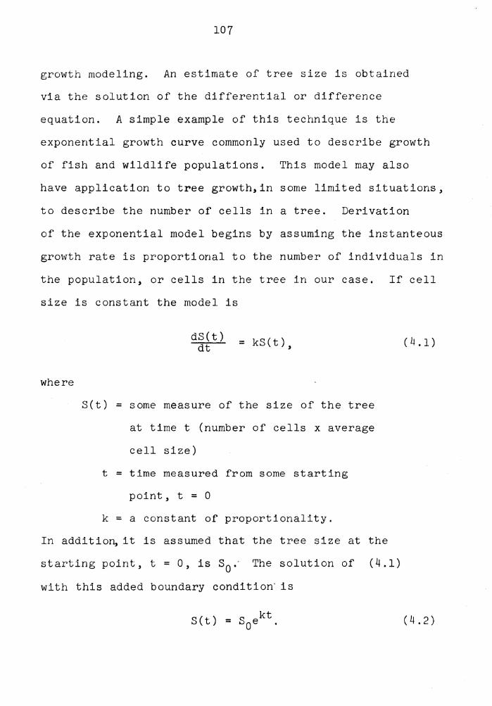
107
growth modeling. An estimate of tree size is obtained
via the solution of the differential or difference
equation. A simple example of this technique is the
exponential growth curve commonly used to describe growth
of fish and wildlife populations. This model may also
have application to tree growth,in some limited situations,
to describe the number of cells in a tree. Derivation
of the exponential model begins by assuming the instanteous
growth rate is proportional to the number of individuals in
the population, or cells in the tree in our case. If cell
size is constant the model is
where
dS(t) dt = kS(t),
S(t) = some measure of the size of the tree
at time t (number of cells x average
cell size)
t = time measured from some starting
point, t = 0
k = a constant of proportionality.
In addition, it is assumed that the tree size at the
starting point, t = 0, is s0 .' The solution of ( 4 .1)
with this added boundary condition· is
(4.1)
( 4. 2)
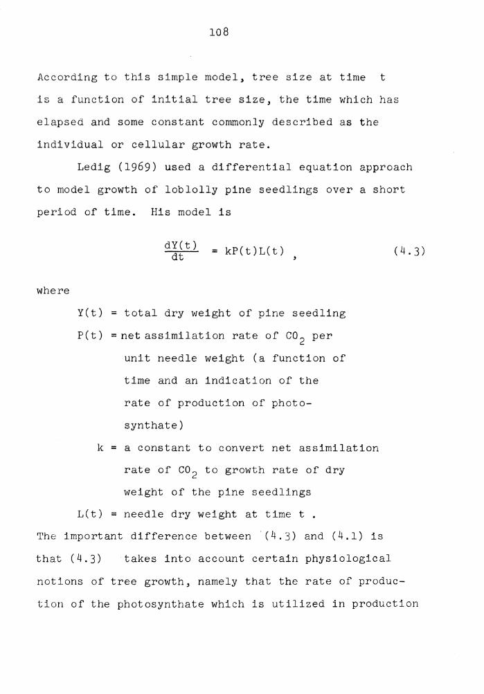
108
According to this simple model, tree size at time t
is a function of initial tree size, the time which has
elapsed and some constant commonly described as the
individual or cellular growth rate.
Ledig (1969) used a differential equation approach
to model growth of loblolly pine seedlings over a short
period of time. His model is
where
dY(t) dt = kP(t)L(t)
Y(t) = total dry weight of pine seedling
P(t) =net assimilation rate of co 2 per
unit needle weight (a function of
time and an indication of the
rate of production of photo-
synthate)
k = a constant to convert net assimilation
rate of co 2 to growth rate of dry
weight of the pine seedlings
L(t) = needle dry weight at time t .
The important difference between (4.3) and (4.1) is
that ( 4. 3) takes into account certain physiological
( 4. 3)
notions of tree growth, namely that the rate of produc-
tion of the photosynthate which is utilized in production

109
of new needles can vary with time and genetic structure
of the seedlings. Other stand variables that would also
affect P(t) and L(t) but which were controlled
in Ledig's experiments are season, weather, site index,
and competition.
The model developed by Ledig was expanded by
Promnitz (1972) to describe the growth of individual
parts of trees such as crown, bole and roots. Promnitz
uses a system of differential equations, each similar in
nature to the model developed by Ledig, to describe the
dry weight growth and yield of each plant part. Both
Ledig and Promnitz modeled tree seedling growth only
over a short period of time (less than six months).
Ledig and Promnitz indicated that their models
might be applied to tree growth for more than one growing
season. However, certain difficulties arise when
attempting to apply these models to plantation grown
trees for up to thirty year periods. Direct measurement
of model components such as net assimilation rate of co 2
for large trees is difficult or impossible. Control of
conditions such as the effect of weather, site and
genetic stock is prohibitively expensive. However, the
incorporation of tree physiology considerations into
growth and yield models is desirable.

110
Past Application of Differential Equation Models to Growth and Yield Prediction
Clutter (1963) applied the concept of a differential-
integral relationship between growth and yield to the
direct multiple linear regression approach of yield
prediction. Similar work has been presented by Schaegel
and Kulow (1969), Moser and Hall (1969), and Moser .(1972,
1974). When considering growth and yield models Clutter
defined compatible as: "Such models are here defined
as compatible when the yield model can be obtained by
summation of the predicted growth through the appropriate
growth periods, or more precisely, when the algebraic
form of the yield model can be derived by mathematical
integration of the growth model." The relationship
Clutter described is embodied in (4.1) and (4.2)((4.1)
describes growth rate and (4.2) is the yield model).
To avoid pitfalls, however, growth rate and growth
must be rigorously defined. In this presentation, growth
rate is defined as the first derivative of yield, that is
the instantaneous rate of change of the size of the tree.
Growth is the change in size of a tree over some fixed
time period, usually one year begining in the spring and
ending in late summer or early fall. These definitions
can be applied to a stand of trees as well as an indivi-
dual tree. Therefore growth rate can be modeled with
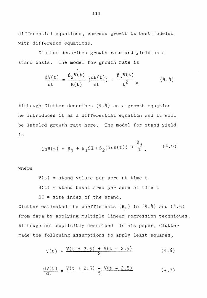
111
differential equations, whereas growth is best modeled
with difference equations.
Clutter describes growth rate and yield on a
stand basis. The model for growth rate is
d V ( t ) = f3 2 V ( t ) ( dB ( t ) ) ( 4. 4) dt B(t) dt
Although Clutter describes (4.4) as a growth equation
he introduces it as a differential equation and it will
be labeled growth rate here. The model for stand yield
is
( 4. 5)
where
V(t) = stand volume per acre at time t
B(t) = stand basal area per acre at time t
SI = site index of the stand.
Clutter estimated the coefficients ($.) in (4.4) and (4.5) l
from data by applying multiple linear regression techniques.
Although not explicitly described in his paper, Clutter
made the following assumptions to apply least squares,
V( t) V(t + 2.5) + V(t - 2.5) = 2 ( 4 • 6 )
dV(t) V(t + 2.5) - V(t - 2.5) = dt 5 (4.7)

B(t)
dB(t) dt =
112
B(t + 2.5) + B(t - 2.5) = 2 ( 4 • 8)
B(t + 2.5) - B(t - 2.5) 5 ( 4 . 9)
These assumptions were made to accomodate the data which
consisted of permanent plots remeasured every five years.
Clutter justified this procedure with the statement:
"with growth periods of only five years, however, it
is felt that the errors introduced by this approximation
are inconsequential." It is interesting to note that
Ledig detected large differences in growth rate within a
single growing season; surely great differences in growth
rate occur within a single year as the growth rate is zero
during the winter months.
A more logical approach would be to obtain a growth
model from the first difference of yield equation (4.5).
Such an approach is complicated by the log transform used
in the y5eld equatlon, since the first difference of
log(X) with respect to X is not as simply evaluated as
is the second derivative, but this slight increase in the
effort of obtaining the model should be off-set by less
stringent assumptions when fitting the data. Such an
approach was suggested by Burkman (1962). He defines
growth and yield in the following manner. "Unless other-
wise specified, growth, for the purposes of this paper, is
periodic net annual incrAment. Growth can be in basal
113
area, cubic feet, cordwood or board feet. Yield is
defined as the summation of a number of net annual
growth increments. 11
Another problem encountered by Clutter is that
although the functional forms of his yield and growth rate
equations are compatible, the estimates of the coefficients
in the equations are not. That is, s2 in (4,4)
may not be equal to s2 in (4.5). Sullivan and
Clutter (1972) suggested an estimation procedure which
overcomes this problem. Although Sullivan and Clutter
add a random error term to each equation, this and all
preceding models in this chapter do not make reasonable
and systematic allowEnce for the stochastic nature of
growth and yield of forest stands.
A Stochastic Approach to Modeling of Growth and Yield
A basic problem encountered with the above approaches
is their deterministic nature. Tree growth is dependent
upon weather which must be considered a random effect as
it certainly cannot be accurately forecasted. The site
quality of the land on which each tree is planted may
vary widely over small areas, especially in the Piedmont
region. These variations, termed microsite, cannot be
easily detected and quantified, and so must be treated as
a random element. The genetic make-up of planting stock
is generally unknown, although in some cases only a few
114
improved genetic types are planted. All these effects,
their interactions, and interactions between the trees
themselves make a strong case for the use of a stochastic
model for tree growth and yie~d. The approach of stochastic
difference equations will be developed in this paper.
Although it is impractical to determine the age of
a tree closer than to the nearest year, it is practical
to measure yearly growth of the bole and larger limbs.
Trees grown in temperate regions contain annual rings,
which are the result of differences in cell size. Wood
cells produced in the spring are larger than those
produced in late summer. The result is a pattern of
concentric circles when the tree is cut along the
horizontal plane, which can be used to determine yearly
diameter growth. When the tree is cut along the vertical
plane a series of converging lines result, which can be
used to determine yearly height growth. The study of
these tree rings is called dendrochronology and is often
concerned with the use of an~ual rings as a record of
weather conditions. Tree rings will be used here as
justification for a model based on yearly tree growth.
A simple model can be developed from the
assumptions implicit in (4.1), namely that growth is
proportional to size. The corresponding difference
equation would be

115
~S(t) = S(t) - S(t -1) = kS(t - 1) . ( 4 . 10)
The solution to the difference equation 4.10 with the
boundary condition S(O) = s0 is
S(t) = s0(1 + k)t. (4.11)
A stochastic element can be added to (4.10) by
allowing k, the cellular growth, to vary from year to
year,
~S(t) = XtS(t - 1).
The solution to (4.12) depends on the distribution
of Xt. If the Xt are independent and identically 2 distributed with mean µ and variance a ,the limiting
distribution of S can be determined. This assumption
( 4. 12)
might be valid if the variability of Xt is due largely to th the weather the t year. Cramer(l946) determines a
solution to (4 .12) by first solving .for Xt ,
X = ~S(t) = t S(t-1)
S'(t') - S(t - 1 ) S(t - 1) '
(4.13)
then summing both sldes of the equality with respe~t to
L. '
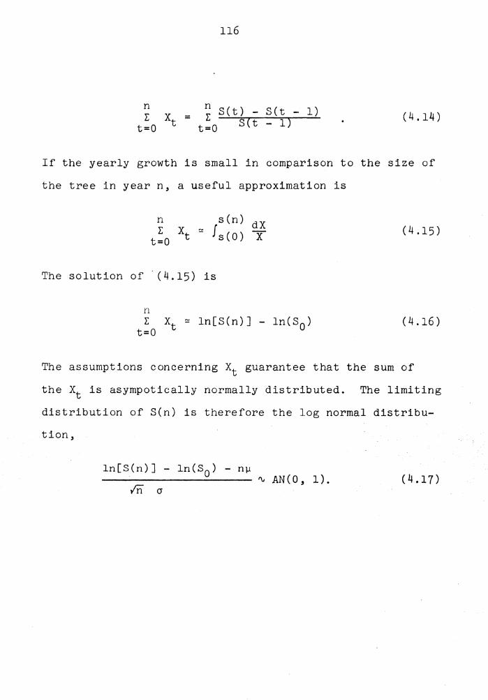
116
= ~ S(t) - S(t - 1) t=O S(t - 1) (4.14)
If the yearly growth is small in comparison to the size of
the tree in year n, a useful approximation is
s(n) ~ f s ( 0) dXX
The solution of · (4.15) is
n ~ xt ~ ln[S(n)J - ln(s0 )
t=O
(4.15)
(4.16)
The assumptions concerning Xt guarantee that the sum of
the Xt is asympotically normally distributed. The limiting
distribution of S(n) is therefore the log normal distribu-
tion,
ln[S(n)] - ln(s0 ) - nµ ~~~~~~~~~~~ ~ rn a
AN ( O, 1). (4.17)

117
Derivation of the Transformed Normal Diameter Distribution
The transformed normal distribution mentioned in
earlier chapters is a generalization of the model
described by (4.17). The growth in a particular
year might not be proportional to the size of the tree,
but to the size raised to some power, say C. The
difference equation describing this phenomenon is
6S(t) = Xt[S(t - l)]~ (4.18)
The power, C, could be interpreted as the effect of
competition on tree growth. A tree grown with no competi-
tion from surrounding trees would not be as limited in
water, nutrient, co 2 and sunlight intake as a tree grown
in close proximity to neighboring trees. The intake of
the open grown tree would be roughly proportional to the
size of the tree. A larger tree would have a larger
crown and could utilize more sunlight. A similar argument
could be applied to the other components of growth.
Increases in competition would give even greater advantage
to the larger trees. Not only is the smaller tree limited
by the size of its crown and root system, but it is
further limited by competition with surrounding trees.
Therefore we would expect C to be small for open-grown
trees, and to increase as competition increases. The
solution to (4.18)is obtained in the same manner as (4.12)
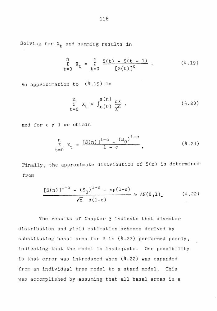
118
Solving for Xt and summing results in
n n L Xt = L
t=O t=O S(t) - S(t - 1)
[S(t)]c
An approximation to (4.19) is
s(n) ~ f s(O) ~~
and for c i 1 we obtain
1-c ~ [S(n)Jl-c - (So)
1 - c 0
(4.19)
(4.20)
(4.21)
Finally, the approximate distribution of S(n) is determined·
from
[S(n)]l-c - (s0 )l-c - nµ(l-c) ~~~~~~~~~~~~~~~ ~ AN(0,1) 0 rn a(l-c)
The results of Chapter 3 indicate that diameter
distribution and yield estimation schemes derived by
(4.22)
substituting basal area for S in (4.22) performed poorly,
indicating that the model is inadequate. One possibility
is that error was introduced when (4.22) was expanded
from an individual tree model to a stand model. This
was accomplished by assuming that all basal areas in a

119
stand are independent and identically distributed
according to (4.22). This may not be true since all
the trees in a stand are exposed to the.same weath~r
conditions. J,t least part of the randomness explained
by Xt is due to weather effects. Since the basal areas
of trees in a stand each depend on a set of random
variables {Xt} and sets of random variables are correlated
due to the common weather effects, perhaps the basal
areas of trees in a forest stand are also correlated,
violating the assumption made to develop the diameter
distribution and yield estimation schemes. An approach
which circumvents this weakness is developed in the
remainder of this chapter.
A Stochastic Model for Open-Grown Loblolly Pine
Competition for growing space in stand-grown trees
is a little understood phenomenon which complicates the
modeling effort. Competition effects will not be
considered initially to simplify derivation of the model.
The effect of competition on the open-grown tree model
will be considered in a later section. A model pertaining
to the growth of the 81 open-grown trees described in
Chapter II is derived in this section.
An implicit assumption of the stochastic models
derived in the previous section is that tree growth is
120
a Markov process, i.e., given the present size of
the tree, future growth is statistically independent of
past growth. The independence of the Xt and the form
of the difference equations imply that tree growth as
modeled is a Markov process. Consideration of this and
certain physiological aspects indicate that a good measure
of tree size is the ordered pair consisting of the tree
height and basal area.
Prediction of bole volume is the primary objective of
this modeling effort, and it was demonstrated in
Chapters 1 and 2 that bole volume is highly correlated
with the product of height and basal area. Growth of
tree boles is the result of activity of two meristems.
Height growth results from activity of the primary
meristems at the tip of the highest shoot of the tree.
Basal area growth is the result of activity of the
secondary meristem often ·referred to as the cambium,
located just under the bark of the tree. The processes
involved in growth of each of these areas is different
although the activity of the two meristems is correlated.
Finally, correlation between tree height and basal area,
and crown size (an important factor in the growth model
since photosynthesis takes place in the tree crown)
is high, as can be seen from Table 4.1. The difference
equations will be constructed in a manner which ensures
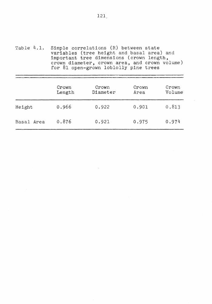
121
Table 4.1. Simple correlations (R) between state variables (tree height and basal area) and important tree dimensions (crown length, crown diameter, crown area, and crown volume) for 81 open-grown loblolly pine trees
Height
Basal Area
Crown Length
0.966
0.876
Crown Diameter
0.922
0.921
Crown Area
0.901
0.975
Crown Volume
0.813
0.974
122
that the ordered pair (height, basal area) is a Markov
process.
The open-grown tree growth model is further
simplified by considering height alone as a Markov process.
Figure 4.1 indicates that over long periods of time
height growth is nearly linear. This assumption also
has physiological support. The primary meristem is
located at the tip of the crown and so the proximity to
the photosynthate producing crown does not change as is
the case with the other meristems. This would indicate
that height growth is relatively constant over time and
only depends on random fluxuations due to weather. Over
longer periods of time height growth is reduced, perhaps
due to the increased effort required to move water and
nutrients to the tip of the tree. The concentration of
photosynthate in the tree, particularly at the apical
meristem, also influences height growth. This concentra-
tion should be proportional to the crown ratio, the
proportion of the bole of the tree supporting foliage.
This ratio is constant over a wide range of open grown
tree sizes as illustrated by Figure 4.2. The relationship
between tree height and crown length is a straight line
through the origin, with a small amount of residual
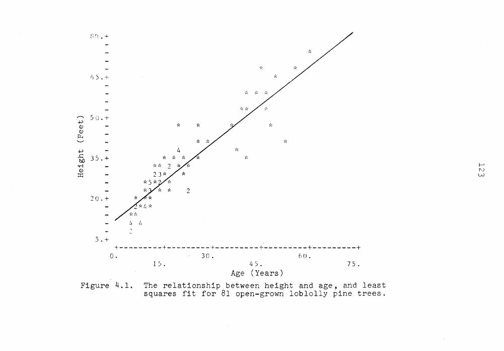
}~ (! • +
-;,'~
r,s.+ *
,.-... Su.+ .µ (J) (J)
µ.. '-"'
.µ
..c: 35.+ bO or-I - -;,," ?/.* (J) -
::r:: - 23* *
20.+ - /1~ - -
!. Li > - -
5. + +---------+---------+---------+---------+---------+
0. 30. 6 () . l r, 4 5 . 7 5.
Age (Years) Figure 4.1. The relationship between height and age, and least
squares fit for 81 open-grown loblolly pine trees.
I-' f',)
w
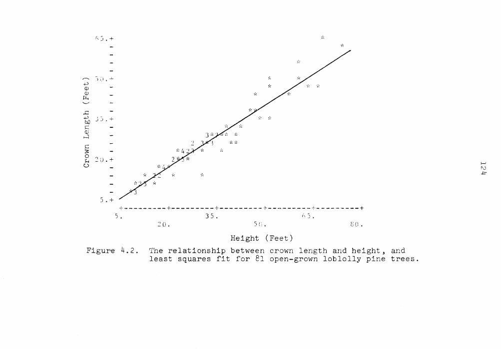
(--. .) . + -).:
~) ;_i • ~~ .µ <I> <I> µ..
......,
..c
.µ I•: I
bD J_J.l"
c: Q)
>-1
c: :;: 0
~u.+ H ~::.? 0
5. + +---------+---------+---------+---------+---------+ ) . 3 5. ;", 5.
:.: 0. 5 (} . l;'I" t..i lJ •
Height (Feet) Figure 4.2. The relationship between crown length and height, and
least squares fit for 81 open-grown loblolly pine trees.
I-' I\.) ..i:::-
variation. This can be contrasted with Figure 4.3
which illustrates the same phenomenon in stand grown
trees. The scattering of data points indicates that
crown ratio is not constant in stand-grown trees. One
of the most important effects of competition is the
resulting decrease in crown length, which results in less
photosynthate being produced, and the accompanying
decrease in tree growth.
The arguments listed above support the use of the
following model for height growth of open-grown trees,
6H(t) = H(t) - H(t - 1) = Xt. (4.23)
This stochastic difference equation describes annual
height growth as a single random variable, Xt. Year to
year randomness is a result of weather conditions. The
distribution of Xt is determined by the genetic make-up
of the tree and_tbe site upon which the tree is planted.
The solution to (4.23) is that the current height of the tree is the summation of the yearly growth of the
tree,
A H (A) = L: Xt
t=l (4.24)

-! . .. , ii+ ., - ..
•) -~~ ') • :; +
,.-.. ..µ (!)
-,'; ')
\1) r=..
;':. ..,,, ,__, :0: ". - ;:+ * * -;;;,"'.'·:
..c: * ;1\ * * ') '- 22 * ..µ OD ;': 2 ****-::. _5*;':
s:: ;": ;": ;'c **3;'2 * 3 )< * Q) ....:i * ;': 2* s:: 2 l. !J+ ·k
:s: * * 0 H
0 * .;, 3 **** :~: ;'\
~ .. {. \) + ,5J52 *3*224*4*42423 * ~
- *J4*~R*4J *** 2 k* 2 * * * 32 1 * * * ~
* i. '..~ ') ;'\ * * ;'c
/ • f'.t ~- ,,
·!----------+---------+---------+---------+---------+c:1 15. 45. 75.
1 (). r, 0 . 90.
Height (Feet) Figure 4.3. The relationship between crown length and height, and
lea8t squares fit for 477 stand-grown loblolly pine trees.
:__J r'-) (.T\
127
An estimate of the expected value of Xt is the sample
average,
A ~ Xt I A = H ( A ) I A .
t=l (4.25)
Empirical estimates of higher moments and the distribution
of Xt is prohibited by the nature of the open-grown data.
Only a single height-age measurement was made for each
tree (a unique combination of genetic make-up and growing
site). Therefore an estimate of the variance of Xt must
be based on a single observation. This problem could be
overcome if annual growth data were available. Such data
would consist of the yearly height of single trees. This
type of data could be obtained by sectioning older trees
and measuring growth as recorded by the annual rings.
A model which takes into account the additional
work required to transport water from the roots to the
apical meristem as tree height increases is described by
the following simple linear expression,
~H(t) = xt - SoH(t - 1). (4.26)

128
A linear approximation implies that the work required to
transport the water increases linearly with tree height.
The solution to the stochastic difference (4.26)
is
H(A) (4.27)
The value of Bo may vary from tree to tree due to
differences in genetic make-up and microsite; hence, the
estimation of Bo and the moments and distribution of Xt
is again precluded by the nature of the open-grown data.
Individual tree height growth data would yield such estimates.
This model would be applicable to height growth of open-grown
trees over longer period of time (greater than thirty years).
Basal area growth is largely dependent on the amount
of photosynthate produced by the tree and the proximity
of themeristern producing the basal area growth to the site
of photosynthate production. The site of this production
is the tree crown, and so the amount of photosynthate
produced should be proportiorial to crown size. Sunlight
is one of the primary requirements of the process, and so

129
production ntight be proportional to the amount of crown
surface directly exposed to sunlight. Crown shape is
approximately conical, so crown area (the surface area
of the tree crown exposed to direct sunlight) is nearly
proportional to the product of crown width and crown
length. Figures 4.2 and Li.4 illustrate that both crown
length and crown width are proportional to height in open-
grown trees. The crown ratio of open-grown trees is
large (over eighty percent of the height of the trees
contains branches) resulting in close proximity of the
meristem producing basal area growth to the tree crown.
These arguments indicate that the relationship between
basal area growth and height squared is linear,
~B(t)
Solving for basal area results in
A B(A) = L [S 0 + S1H(t) 2 J
t=l
(4.28)
(4.29)
The nature of the data preclude estimation of Bo and B1
which may vary from tree to tree due to differences in
genetic make-up and microsite. The following assumptions
permit evaluation of this basal area growth model.
Adopting the height growth philosophy of (4.24) and
treating Xt as a constant rather than a random variable
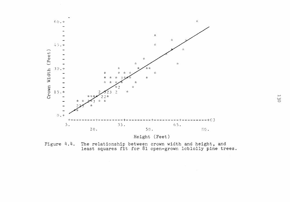
.µ Q) Q) µ:. '--'
(i().+
!.; ~). +
.c 3'.J.+
.µ 'O -rl :::;: c :s: -0 1). + H
0
(). +
;.;
+---------+---------+---------+---------+---------+C3 5. 3 5. (1 5 .
2 (). so. [.; 0 .
Height (Feet) Figure 4.4. The relationship between crown width and height, and
least squares fit for 81 open-grown loblolly pine trees.
f-J w 0
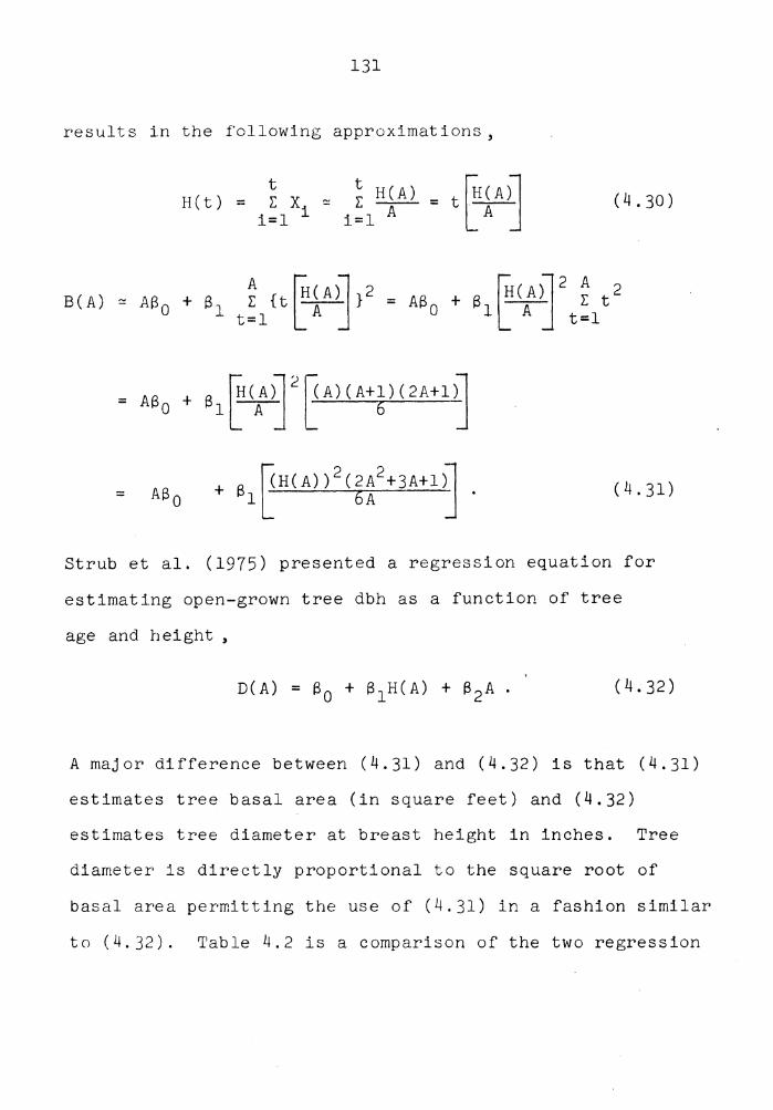
131
results in the following approximations,
t H(t) = l: Xi ~
i=l ~ H ( A) = t liiA( A)]
i=l A [ ] ( 4 • 30)
B(A) ~ AS + s ~ { t IB (A)] } 2 = AS + f3 rir ( A)] 2 ~ t 2 0 1 t=l [A J 0 1 l A J t=l
= (4.31)
Strub et al. (1975) presented a regression equation for
estimating open-grown tree dbh as a function of tree
age and height ,
(4.32)
A major difference between (4.31) and (4.32) is that (4.31)
estimates tree basal area (in square feet) and (4.32)
estimates tree diameter at breast height in inches. Tree
diameter is directly proportional to the square root of
basal area permitting the use of (4.31) in a fashion similar
to (4.32). Table 4.2 is a comparison of the two regression
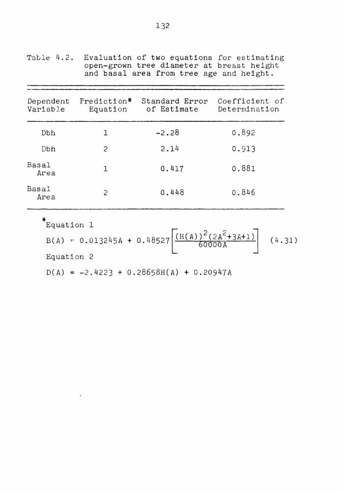
132
Table 4.2. Evaluation of two equations for estimating open-grown tree diameter at breast height and basal area from tree age and height.
Dependent Prediction* Standard Error Coefficient of Variable Equation of Estimate Determination
Dbh 1 -2.28 0.892
Dbh 2 2.14 0.913
Basal 1 0.417 0.881 Area
Basal 2 0.448 o.846 Area
* Equation 1
B ( A) ,. 0 • 0 13 2 4 5 A + 0 • 4 8 5 27 ~ H ( A ) ~ ~ 6 6 ~: + 3 A+ l )j ( 4 • 31 )
Equation 2
D(A) = -2.4223 + 0.28658H(A) + 0.20947A

133
equations, listing a measure of the amount of variation
unexplained by each regression equation (the standard
error of estimate) and the percentage of the total
variation of the dependent variable explained by the
regression equation (the coefficient of determination).
This comparison is performed when tree diameter and tree
basal area are each the variable of interest.
The first two rows of Table 4.2 represent a
comparison of the two regression equations when diameter
at breast height is predicted from tree height and age.
Tree dbh is predicted from (4.31) by first estima-
ting s0 and s1 by using least squares and the data
collected from the 81 open-grown trees. These estimates
were substituted for s0 and s1 in equation(4.3]. This
equation is used to estimate tree basal area from tree
height and age. Estimated tree diameter is obtained by
multiplying the square root of estimated basal area by the -
constant 13.54. Least squares estimates of s0 , S1 ,
and s2 substituted into (4.32) result in an equation
which can be used to estimate tree diameter directly from
tree height and age. The sum of the squared differences
between observed tree diameter and estimated tree diameter
was calculated for each prediction equation. The
coefficient of determination and standard error of
estimate was calculated from the sum of squared differences.
134
A similar approach was used to obtain rows three
and four of Table 4.2. The dependent variable was basal
area for this part of the comparison, Equation (4.31) was
used to estimate tree basal area directly from tree height
and age. Equation (4.32) was used to estimate tree
diameter from height and age. Estimates of basal area
were obtained by multiplying the square of diameter by the
constant 0.005454. The sum of squared differences between
observed and estimated tree basal area was calculated for
each prediction equation. These sums of squared differences
were used to calculate the coefficients of determination
and standard errors of estimate contained in rows three
and four of Table 4.2.
Table 4.2 indicates that (4.32) is the
preferred equation for estimating tree dbh, and (4.31)
is the preferred equation for estimating tree basal
area. The slight advantage shown by each equation is
probably due to the least squares estimation procedure
used to determine the coefficients, one equation is the
least squares fit for dbh, the other for basal area. This
suggests that the assumptions made to develop (4.24)
and (4.28) are reasonable, since an adequate estimation
model resulted from these assumptions.
Equations (4.24) and (4.28) could be used to model
growth of open-grown trees. Use of this model depends on
assuming some probability distribution for Xt and

135
estimation of the parameters a0 and a 1 . If a random
sample of open-grown trees is considered, ao and al
are also random variables. Hence, the value of a0 and
a1 vary with each measurement of tree basal area,
height, and age. Estimation of parameters and probability
distributions is again prohibited by the nature of the
data. Data with multiple observations over time would
permit estimation and subsequent application of these
types of models.
Stochastic Modeling of Stand-Grown Trees
Many of the assumptions valid to the development of
the open-grown tree model are not applicable to
competition-grown trees. The complicating effect of
competition results in scatter diagrams similar to Figure
4.3 when data from a broad range of stand variables are
examined. Data from the sectioned trees (two on each
plot) described in chapter 2 were available for use in
modeling height growth of stand-grown trees. These data
consisted of age height pairs for each tree. Due to
the method of collection of the data height measurements
are accurate only to the nearest four feet. When these
crude data were examined, a linear relationship between
height and age was noted. Therefore (4.24) is
applicable to competition grown trees, however the
136
distribution of Xt is further modified by competitive
stress. Strub et al. (1975) presented argument$ Wh1ch
indicate that height growth of open grown trees is
generally less than height growth of trees grown under
competitive stress when all other variables are
constant. The crude nature of the height data hinders
estimation of the distribution of Xt under different
stand conditions.
Modeling of basal area growth in competitive-grown
trees is even more limited by the nature of the data. The
relationship between height and crown size is weak. The
distance from the area of growth to the crown of the
tree varies with stand conditions. These arguments
indicate that (4.29) must be modified to add flexibility
needed to model the growth of trees grown under competitive
stress. The modeling efforts of Ledig (1969) described
earlier in this chapter suggest an appropriate solution
to this problem might be
(4.33)
The functions L(t) and P(t) will be discussed in detail
in the next two sections.
Effective Crown Area
In 0.33)L(t) is the area of the crown exposed to
direct sunlight. The effective crown area of open-grown

137
trees can be determined frcm the crown width and crown
length if a conical crown is assumed, since the entire
surface of the open-grown tree crown is exposed to
direct sunlight. This is not true of trees grown under
competitive stress. The top of the crown is exposed to
direct sunlight and the bottom of the crown is shaded by
neighboring trees. The result of this shading is that
the needles on the lower branches have a much lower rate
of photosynthate production than the needles located
near the top of the tree. In fact, the rate of photo-
synthate production in lower branches is often so low
that more photosynthate is used in respiration than is
produced in photosynthesis, hence the net rate of
production is negative. The effective crown area, that
is the area of the crown which is actively engaged in net
positive production of photosynthate is located in the
upper regions of the tree. A method of estimating the
effective crown area can be derived from the results of
Strub, et al. (1975). This method was based on compari-
sons of growth of open-grown and stand-grown trees.
Diameter growth of open-grown and stand-grown lob-
lolly pine trees was compared by Strub, et al. They
determined that the diameter growth of stand-grown trees
begins to differ from that of open-grown trees at approxima-
tely the same time Uw t the crown competition factor reaches
100. A detailed description of the crown competition

138
factor (CCF) can be found in Krajicek et al. (1961).
The crown competition factor is based on the relationship
between crown diameter and dbh of open-grown trees. This
relationship is linear and the crown diameter of open-
grown trees can be accurately estimated from dbh by
means of simple linear regression. The vertical
projection of the crown onto the ground is simply rr
multiplied by the crown radius squared. These two
relationships can be used to estimate the projected
area occupied by the crown of any open-grown tree of
specified dbh. CCF is determined by associating with
each tree in the stand the projected crown area (termed
maximum crown area) of an open-grown tree with the same
dbh as the competition-grown tree. The CCF is the ratio
of the sum of the maximum crown areas to the area of the
land occupied by the stand, expressed as a percentage. A
CCF of 100 would indicate that if the crowns of all the
trees in a stand occupied an area equal to the area
occupied by open-grown trees of the same dbh, the land
would be exactly covered by tree crowns. The results of
Strub et al. indicate that after this point in time the
diameter growth of stand-grown trees differs from that
of open-grown trees.
This change in growth patterns might indicate that
when CCF reaches 100 the effective crown area of the
139
stand-grown trees reaches a maximum. Up to this time
(the time at which CCF reaches 100) the growth of the
trees would follow the same pattern as open-grown
trees, described by (4.28). Once CCF surpasses 100,
growth is the result of activity in the effective crown,
the area of which remains approximately equal to crown
area when CCF reaches 100. Effective crown area then
depends on the age at which the CCF reaches 100.
Figure 4.4 indicates that crown diameter is
proportional to height in open-grown trees. Projected
crown area should then be proportional to the square of
height. This phenomenon is illustrated by Figure 4.5.
Regression was used to estimate the average projected
crown area from tree height ,
PCA(t) = 0.39401 H(t) 2 ( 4. 34)
The coefficient of determination is 80.7 percent and the
stfil1dard error of estimate 233.8 square feet. The product
of average projected crown area and the number of trees
per acre results in the land area occupied by tree
crowns when all trees are open-grown. The CCF of N open-
grown trees is estimated by
CCP(t) = 0.39401 N H(t) 2/43560. (4.35)

J oor1. + * -
......... .µ <lJ v ·1 4 on.+ r:;:. ~ ..
Q) i.:.t Cd :::s O' U) 1 ,, (\ () + ..__, () ·' . . ct! Q) i.:.t ~
s:: 1200.+ :s:
0
*/ ~·: -H
u -'d <l.l .µ CJ
F:y 00. + Q) "r-:> 0 i.:.t 0-. -
-').+
+---------+---------+---------+---------+---------+CJ o. 3uoo. 6oon.
l) 00. 4500. 7 500.
Height Squared (Square Feet) Figure 4.5. The relationship between crown area and the square of
height, and least squares fit for 81 open-grown loblolly pine trees.
I-' ,_ 0

Occupied land area must be divided by the number of
square feet in an acre (43560) since projected crown
area is measured in square feet. The age at which CCF
reaches 100 is determined by substituting 100 and solving
4. 35 for t. A solution is .o~~~.in.~d by approximating
H(t) with tHd/A, an assumption similar to (4.30),
(4.36)
The effective crown area of stand-grown trees is
equivalent to that of open-grown trees up to age Ac' and
remains fixed at the same value after age A , c
A = ~32.5 ~· c H li'f
d
(4.37)
Where [ · ]] indicates the greatest integer function.
As previously discussed, crown area is proportional
to the square of height in open-grown trees,
2 CA(t) = a2H(t) . (4.38)
The effective crown area of competition grown trees is
described by
ECA(t) t < A c t > A c
(4.39)
142
The area of the crown exposed to direct sunlight, L(t),
is proportional to effective crown area, ECA(t),
L(t) = yECA(t). (4.40)
Photosynthate Allocation
The term P(t) in (4.33) represents the proportion
of the net photosynthate produced which results in basal
area growth. The amount of photosynthate utilized in
basal area growth is a function of the amount of photo-
synthate which reaches the secondary meristem at breast
height. Transport of photosynthate is then of primary
importance to the determination of a proper expression
for P(t).
Photosynthate is transported by long thin strings
of hollow straw-like cells called phloem, which run from
the tip of the tree to the roots and along tree branches.
Phloem is located between the cambium and the bark of the
tree. The phloem cells are water filled and transport
materials such as photosynthate from the crown to the
roots. Cambial cells located adjacent to the phloem
intercept photosynthate on its downward route in the
phloem. If the overall concentration of photosynthate in
a tree is low, a large proportion of the photosynthate
produced would be intercepted by cambial cells located
in or close to the crown of the tree. As the concentra-
tion photosynthate in the tree is increased, the cambial
tissue near the top of the tree reaches some saturation

143
point, that is some limit to the amount of photosynthate
which can be utilized by the cell is reached. A larger
amount of photosynthate then reaches cambial cells
located near the base of the tree.
This argument indicates that the proportion of
photosynthate allocated to basal area growth is propor-
tional to the concentration of photosynthate in the tree
bole. This concentration should be approximately
proportional to the ratio of the length of the effective
crown to the height of the tree. Figure 4.3 indicates
that the crown length of open-grown trees is proportional
to height. The preceding discussion indicates that
effective crown length (the length of the portion of the
crown which has a positive net effect on the production
of photosynthate) of stand-grown trees would be equal to
total crown length until CCF reaches 100. The effective
crown length after CCF surpasses 100 would be somewhat
less than total crown length and approximately equal to
crown length at the time CCF reaches 100. If a is the
ratio of crown length to height in open-grown ~re~s,
P(t) can be modeled as
(a CL( t) = S3 t H(t) < A c P(t)
= (a (4.41) CL(Ac) S3 H(Ac) H(t) = H(t) t > A c .

144
The symbo 1 B -, represents the product of the crown ratio :::i
of the tree if it were open-grown and some constant to
convert effective crown ratio to the proportion of photo-
synthate which reaches the camoium at breast height.
A Description of Basal Area Growth in Stand-Grown Trees
Substituting (4.39), (4.40), and (4.41) into
(4.33) an expression for basal area growth is obtained,
(So 2 +yf3 1s3s2H(t) t < A c
6B(t) ( 4. 42) :: ) I ~3H~~~ 2 \ Bo t yS 1 --i:rm_J B2H (Ac) t > A . c
Combining parameters y, s1 , B2 and s3 results in
f So ')
+ B -"H( t) L t < A 1 c 6B(t) = ( 4. 4 3)
\ .. H(Ac)3 t > A Bo + B1 H(t) c
Equations (4.23), (4.37) and (4.43) can be used jointly to
model growth of individual stand grown trees.
These thr·ee equations contain only a sj_ngle random
element, Xt' the random variable which represents the
effect of weather on tree height growth. When an entire
stand of trees is considered this interpretation changes;
145
are fixed parameters only for a single tree,
and vary from tree to tree in a stand due to changes in
genetic structure and microsite variability. These sources
of variability can be included in the model by substituting
the random variables Y and Z for the parameters a0 and
-- {yy + ZH(t) 2 ~B(t)
+ ZH(Ac) 3/H(~) t > A • c
(4.44)
All trees in the stand are exposed to the same
weather conditions, hence differences between trees and
the resulting height and basal area distributions are
due to differences in the genetic structure of the trees and
microsite changes, not exposure to different weather condi-
tions. Weather would cause varlation in diameter distribu-
tions between stands of trees, since different stands are
separated geographically as well as in time. This
argument indicates that variation between height and
basal areas of trees in a stand does not result from the
random variable Xt. Forest managers would like to
estimate the joint height and basal area distribution for
average weather conditions. The expected value (with
respect to the random variable Xt) of tree height and
146
basal area are of prime interest to the forest manager.
Evaluation of expected tree height from equation
4.23 is straight forward,
The expected value of Xt is represented by µX. The
distribution of Xt may vary from tree to tree due to
differences in genetic make-up of the tree and differences
in microsite. This indicates that for a stand of trees
µX is a random variable, represented here by the symbol
U, and
. (4.46~
A similar approach can be applied to tree basal
areas,
A r Ex[tiB(t)J =
t=l
A r Ex[Y + ZH(t) 2J
t=l A < Ac. ( 4 • 4 7 )
The random variables Y and Z are independent of Xt since
choice of genetic make-up and microsite is independent of
weather, resulting in

147
A EX[H(t) 2 J}
A EX[B(A)] = z:: {Y + z = AY + Z l: EX[H(t) 2 J
t=l t=l
AY + z ~ Ex~ ~ x1 )~ A 2 2 = = AY + z z:: [tax +(tµx) J t=l. i=l t=l
A < A • - c (4.48)
Equation ( 4. 48) describes tree basal areas of open-grown
trees and stand-grown trees in which the CCF has not
yet reached 100. 2 Again µX and ox (the mean and variance
of Xt) may vary from tree to tree and will be represented
by the random variables U and V,
The expression for expected basal area of stand-grown
trees after CCF surpasses 100 is more difficult to
evaluate,
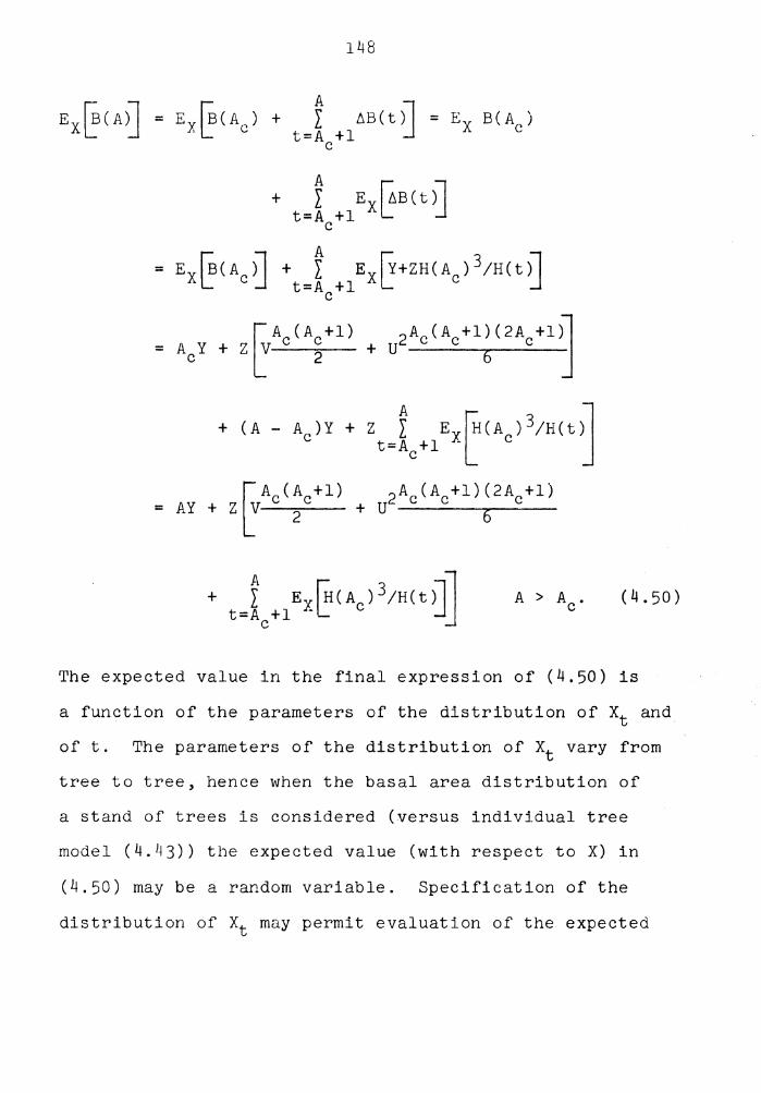
148
+ t EX~B(t)l t=A +l L ~ c
2 Ac(A +l) (2A +l~ + u c c J
A > A . c (4.50)
The expected value in the final expression of (4.50) is
a function of the parameters of the distribution of Xt and
of t. The parameters of the distribution of Xt vary from
tree to tree, hence when the basal area distribution of
a stand of trees is considered (versus individual tree
model (4.43)) the expected value (with respect to X) in
(4.50) may be a random variable. Specification of the
distribution of Xt may permit evaluation of the expected
149
value in (4.50). This evaluation would facilitate
further development of this model.
Estimation of Distributions and Parameters in the Basal Area - Height Model
Yield can be estimated if the joint probability
function of tree basal area and height is specified. This
joint probability density function could be estimated
from (4.46), (4.49), and (4.50). Data requirements
for such an estimation procedure are in excess of the
data available for this study. The required data could
be obtained by sectioning trees.
Data could be collected for all trees on some
fractional part of many stands, just as the trees on the
0.1-acre plots were measured for this study. Stand age,
height of the dominant and codominant trees, and the
number of trees per acre should be determined for each
plot. Each tree should then be felled and sectioned to
determine height and basal area at the end of each year
growth from the annual rings. Basal area and height
growth for each of the trees could be measured in this
manner.
Average height growth, µX' and the variance of 2 height growth, a X' over time could be estimated for
each tree from this data. The expected value in
150
(4.49) could be estimated for each tree by substituting
height growth in the ifh year for ~i' The frequency
distribution of the estimates for all the trees on a
plot could be used to determine estimates of the probability
distributions of U, V, and the expected value in the last
expression of (4.50). This data could also be used to
determine the relationship between these probability
distributions and the stand parameters.
The coefficients describing individual tree basal
area growth, ~O and ~l~, in (4.43) could be
estimated for individual trees by applying the least
squares criterion. The distribution of s0 and a 1 ~ within
a stand, that is the distribution of Y and z,would be
estimated by the frequency distribution of the estimates
of s0 and s 1 ~ for individual trees. The relationship
between stand parameters and the distribution of y and
Z could also be examined.
These techniques could be used to derive a
procedure for estimating the expected (with respect to
weather) distribution of basal area and height. The data
set described above would also serve as a check on the
models derived in the previous section.
151
Application of the Basal Area - Height Model to Estimation of Yields of Forest Stands
The procedure described in the previous section
might be used to estimate the joint distribution of tree
heights and basal areas for average weather conditions.
This joint distribution could be used to estimate stand
yield from stand variables. Individual tree yield is
often modeled as a function of tree height and diameter
at breast height squared (which is directly proportional
to basal area). Incorporation of such an individual
tree yield equation into a generalized version of
indirect stand yield equation (2.67) results in a stand
yield estimation procedure based on the joint distribu-
tion of tree height and basal area.
A generalized version of (2.76) requires use of
two sets of class intervals. The variable i indexes
a set of tree basal area classes with class midpoints
B.. The variable j indexes a set of height classes with l
class midpoints Hj. The probability Pij represents the
probability that for a specified set of stand variables,
a tree is in the ith diameter class and the jth height
class. The proportion of the trees in the ith diameter
class and the jth height class which are suitable for
152
the manufacture of a product such as lumber is
represented by Qij" An individual tree volume
equation such as (1.3) is represented by g(Bi' Hj).
Since basal area is directly proportional to the
square of tree diameter at breast height, an equation
which is equivalent to (1.3) is
(4.51)
Stand yield could be predicted by using the rn basal
area classes and the n height classes in the following
fashion,
m n y = N l l pijQiJ.g(Bi, Hj).
i=l j=l (4.52)
Prediction cf Pij would result from approximation of the
joint density function of tree height and basal area as
a function of stand variables just as the probability
density function for tree diameter was predicted as a
function of stand variables. The approximation of the
joint density function (f(B, H)) is integrated over the
range of the 1th diameter class and the jth height class
to obtain Pij'
153
Hj+wh/2 Bi+wb/2
= JHj-wh/2J s1-wb/2 f(B, H)dBdH. ( 4. 5 3)
The width of a basal area class is wb, the width of a
height class is wh. The probability that a tree in the
ith basal area class and the jth height class is suitable
for the production of lumber, Qij' could be estimated
from individual tree data or predicted as a function of
basal area and height by using the same techniques used
to estimate Q •• J
The class-interval-free analog to (2.87)
can be developed by evaluating the limit of (4.52) as the
number of basal area classes (m) and the number of height
classes (n) increase without bound,
m y = lim N >= (4.54)
m-+oo i==l n-+oo
The range of the tree basal area classes (mwb) and the
range of the height classes (nwh) are held constant. The
limits of the range of basal area classes are represented
by Lb and Ub, and the limits of the range of height classes
are Lh and Uh. The interval widths can be described in the
following manner,
154
(4.56)
Substituting (4.52), (4.54), and (4.55) into (4.53)
results in
H j + c uh -Lh ye 2n) ri+(Ub-Lb)/(2m) m n
Lj-(Uh-Li,)/(2n)
v = lim N L: L: J..
m-+oo i=l j=l n-+oo Bi -( ub -Lb) I ( 2m)
f(B, H)dBdHQi .g(B., H.). J l J
(4.57)
Replacing Q .. with a continuous function of B and H, lJ q(B, H) results in
n rj +(Uh-Lh )/(2n) Bi+ ( ub -Lb ) I ( 2m) m
y = lim N L: L: i=l j=l m-+oo
n-+oo H -(U -L )/(2n) Bi-(Ub-Lb)/(2m) j h h
'l'he definition of the multiple integral ensures that (4.59)
has the same limit as (4.58),
m n y = lim N L: L: f(Bi'
m+oo i=l j=l H.)tiB1 LiH.q(B., H.)g(B1 , Hj). (4.59)
J J l J n-1--00

155
The c 1<2.ss interval width wb is represented by llB1 and wh
is represented by b.Hj. If q and g are continuous functions
applic&tion of the definition of multiple integrals results
(4.60)
This class-interval free stand yield equation can be used
to estimate yield from the joint density of basal area
and height.

V. CONCLUSIONS AND RECOMMENDN.PIONS
The comparisons and tests presented in chapter 3
indicate that no proposed diameter distribution estima-
tion technique adequately described the diameter
distribution of loblolly pine plantations for the age,
site and density combinations observed. A logical
approach to the development of a diameter distribution
estimation technique is presented in chapter 4. Such an
approach requires incremental data not currently available.
Consideration of the physiology of individual tree growth
could lead to accurate and biologically sound prediction
equations.
The comparisons presented in chapter 3 a.lso indicate
that indirect yield estimation can be as accurate as direct
yield estimation. The Weibull distribution function,
(2.20), estimation of parameters based on quantiles,
(2.29), (1.10), and (1.11), and yield estimation
based on 1-inch class intervals, (2.76), provides a
simple yet accurate scheme for yield estimation. A more
complex technique which requires extensive use of high-
speed computers is the discrete approximation to diamter
distributions, (2.74) and (2.76). This technique also
provided accurate results. When only total cubic
foot volume and cubic foot volume to a 4-inch merchant-
ability limit were estimated, the Weibull distribution
156
157
function, (2.20), estimators based on the smallest
and average diameter, (2.32), (2.35), and (2.36), and
the class-interval-free yield estimation procedures,
(2.87), provide accurate board foot yield estimates.
Consideration of culmination mean annual increment
also supported use of estimates based on the normal basal
area approach to diameter distribution estimation and the
class-interval-free yield estimation procedures. None
of the other yield estimation schemes conformed exactly
to pr·econceived notions of the behavior of mean annual
increment culmination. These results are also discussed
in chapter 3.
The various methods of yield estimation can
be compared by considering the allowance each technique
makes for the stochastic nature of growth of forest
stands. Sources of variation in growth can be due to
weather effects, microsite and genetic effects, and
differences in stand variables which result in variation
between stands of trees. The manager cannot control
weather, hence, he is usually interested in yield for
some average set of weather conditions. Microsite and
genetic variation results in differences in tree size
and yield within a stand. Stand variables are the only
sources of variation which have been successfully
quantified. Consequently the stand variable variation

158
can be modeled deterministically, while the weather,
microsite, and genetic effects have not been successfully
quantified, hence they contribute to errors in yield
estimation.
The direct method of yield estimation treats the
stand variables in a deterministic fashion. The weather
and other factors are modeled as a single additive
error term which has constant variance over the range
of stand variables. This is an over-simplification of
the many physiological processes which result in varia-
tion in individual tree and stand yield.
The indirect method of yield estimation treats
the stand variables in a deterministic fashion. Microsite
and genetic variation is accounted for by estimating the
diameter distribution. This approach does not make
systematic allowance for weather fluxuations.
The unified method of yield estimation described
in chapter 4 was developed by considering variation due
to weather, microsite and genetic effects, and stand
characteristics. Such a model requires more detailed
input data. If variation in growth between and within
stands, is to be separated, the stand model must be
based on growth data which measures between and within
stand variation. Such data were not available in this
159
study which precluded completion and exact specifica-
tion of the unified method of yield estimation.
The previous argument and comparisons presented
in chapter 3 indicate that the choice of procedure for
estimation of yields of forest stands depends on the
nature of the data available for development of the
procedure. If yield measurements are available for
only a single point in time, as was the case for data
used in this dissertation, the normal basal area approach
to yield estimation presented in chapter 2 should be
used. Equations (2.37), (2.38), (2.41), and (2.42) can
be used to approximate the diameter distribution of
forest stands. The approximate diameter distribution
and individual tree volume equation (2.5) can be
substituted into (2.87) to obtain stand yield estimates.
This procedure provides an accurate estimate of yield
and supplies the forest manager with additional informa-
tion in the form of an approximate diameter distribution.
The procedures developed in chapter 4 should be
used to estimate stand yield if data consisting of
repeated measurements of yield of the same trees at
different ages were available. The biologically based
yield estimation procedure should be applicable to a
wide range of stand variables, and supplies the manager

160
with ~etailed information about individual tree and
stand growth and yield.

LITERATURE CITED
Bailey, R. L. 1972. Development of unthinned stands of P,£.nu..6 Jr.ad.i.a.ta. in New Zealand. Unpublished dissertation. University of Georgia. 67 pp.
Bailey, R. L. and T. R. Dell. 1973. Quantifying diameter distributions with the Weibull function. Forest Science 19:97-104.
Bare, B.· B. 1970. User's Manual for the Purdue forest management game. Center for Quantitative Studies paper 38. University of Washington. 72 pp.
Bennett, F. A. and J. L. Clutter. 1968. Multiple-product yield estimates for unthinned slash pine plantations -- pulpwood, sawtimber, gum. U.S.D.A. Forest Service Research Paper SE-35. 21 pp.
Bliss, C. I. and K. A. Reinker. 1964. A log-normal . approach to diameter distributions in even-aged stands. Forest Science 10:350-360.
Box, G. E. P., and M. E. Muller. 1958. A note on the generation of random normal deviates. Annal of Mathematical Statistics 24:610-611.
Brister, G. H. 1972. A biometrical study of ment of secondary xylem in Douglas fir. dissertation, University of Washington.
the develop-Unpublished pp. 70-104.
Bruce, D. and L. H. Reineke. 1928. The use of alinement charts in constructing forest stand tables. Journal of Agricultural Research 38:289-309.
Buckmar., R. E. Minnesota.
1962. Growth and yield of red pine in U.S.D.A. Technical Bulletin 1272. 50 pp.
161
162
Burkhart, H. E., R. C. Parker, M. R. Strub, and R. G. Oderwald. 1972. Yields of old-field loblolly pine plantations. FWS-3-72. Division of Forestry and Wildlife Resources, Virginia Polytechnic Institute and State University, Blacksburg, VA. 51 pp. ,
Burkhart, H. E., and M. R. Strub. 1974. A model for simulation of planted loblolly pine stands. IN Growth models for tree and stand simulation. Royal College of Forestry, Stockholm, Sweden. pp. 128-135.
Clutter, J. L. 1963. Compatible growth and yield models for loblolly pine. Forest Science 9:354-371.
Clutter, J. L. and F. A. Bennett. 1965. Diameter distributions in old-field slash pine plantations. Georgia Forest Research Council Report No. 13. 9 p~.
Cox, D. R. 1970. The Analysis of Bina!2_ Data. Methuen and Company, London, England. 142 pp.
Cramer, H. 1946. Mathematical methods of statistics. Princeton Mathematical Series, No. 9, Princeton University Press. pp. 218-220.
Davidon, W. C. 1959. Variable metric method for minimization. A.E.C. Research and Development Report, ANL-5990 (Rev.). 21 pp.
Davis, K. P. 1966. Forest management: regulation and valuation. McGraw-Hill Book Company. New York, NY. 519 pp.
Draper, N. R. and H. Smith. 1966. ~plied regression analysis. John Wiley and Sons, Inc., New York, NY. ~07 pp.
163
Dubey, s. D. 1967. Some percentile estimators for Weibull parameters. Technometrics 9, 119-129.
Fletcher, R. and M. J. D. Powell. 1963. A rapidly convergent descent method for minimization. Computer Journal 6:163-168.
Garwood, F. 1941. The application of maximum likeli-hood to dosage mortality curves. Biometrika
32:46-58.
Gibbons, J. D. 1971. Nonparametric statistic:al_ inference. McGraw-Hill Book Company, ~Jew York, NY. 306 pp.
Graybill, F. A. 1961. An introduction to linear statistical models, volume I. McGraw-Hill Book Co., Inc., New York, NY. 463 pp.
Green, J. R., and Y. A. S. Hegazy. 1976. Powerful modified-EDF goodness-of-fit tests. Journal of the American Statistical Association 71:204-209.
Hamilton, David A., Jr. 1974. Event probabilities estimated by regression. U.S.D.A. Forest Service Research Paper INT-152. 18 pp.
Harter, H. L. and A. H. Moore. 1965. Maximum likelihood estimation of the parameters of gamma and Weibull populations from complete and from censored samples. Technometrics 7:639-643.
hush, B., C. I. Miller and T. W. Beers. 1972. Forest Mensuration. Ronald Press Company, New York, NY.
410 pp.
International Business Machine Corporation. 1970. IBM System/360 Scientific Subroutine Package Version III Programmer's Manual. pp. 221-225.
164
Jennrich, R. I., and R. H. Moore. 1976. Maximum likeli-hood estimation by means of nonlinear least squares IN American Statistical Association 1975 Proceedings of the Statistical Computing Section American Statistical Association, Washington, DC. pp. 5 7 -6 5.
Krajicek, J. E., K. A. Binkman and S. F. Gingrich. 1961. Crown competition -- a measure of density. Forest
Science 7:35-42.
Ledig, F. T. 1969. A growth model for tree seedlings based on the rate of photosynthesis and the distribution of photosynthate. Photosynthetica
3:263-275.
Lenhart, J. L. 1972. Cubic-foot yields for unthinned old-field loblolly pine plantations in the interior West Gulf Coastal Plain. Stephen F. Austin State University, Texas Forest Paper No. 14, 46 pp.
Lenhart, J. D. and J. L. Clutter. 1971. Cubic-foot yield loblolly pine plantations in the Georgia Piedmont. Georgia Forest Research Council Report 22 - Series 3. 13 pp.
Lloyd, F. T. 1966. A description of Virginia pine diameter distributions. Unpublished thesis, Virginia Polytechnic Institute and State University. 46 pp.
McGee, C. E. and L. Della-Bianca. 1967. Diameter distributions in natural yellow-popular stands. U.S.D.A. Forest Service Research Paper SE-25. 7 pp.

165
Meyer, W. H. 1928. Rates of growth of immature douglas fir as shown by periodic remeasurements on permanent plots. Journal of Agricultural Research 36:193-215.
Meyer, W. H. 1930. Diameter distribution series in even-aged forest stands. Yale U~iversity, School of Forestry Bulletin 28. 105 p.
Moser, J. W. stand.
1972. Dynamics of an uneven-aged forest Forest Science 18-184-191.
Moser, J. W. 1974. A system of equations for the components of forest growth. IN Growth Models for '11 ree and Stand Simulation. Royal College of Forestry, Stockholm, Sweden. pp. 260-287.
Moser, J. W. and O. F. Hall. 1969. Deriving growth and yield functions for uneven-aged forest stands. Forest Science 15:183-188.
Myers, C. A. 1973. Computerized preparation of timber management plans: TEVAP 2. U.S.D.A. Forest Service Research Paper RM-115, 7 pp.
Navan, D. I. 1971. Timber ram ... a long-range plan-ning method for commercial timber lands under multiple-use management. U.S.D.A., Forest Service Research Paper PSW-70. 22 pp.
Nelson, T. C. 1964. Diameter distribution and growth of loblolly pine. Forest Science 10:105-115.
Neyman, J. and E. S. Pearson. 1928. On the use and interpretation of certain test criteria for purposes of statistical inference. Biometrika 20A:J75-240 and 263-294.

166
Osborne, J. G. and F. X. Schumacher. 1935. The construction of normal-yield and stand tables for even-age timber stands. Journal of Agricultural Research 51:547-564.
Promnitz, L. C. 1972. for tree growth. State University.
A photosynthate allocation model Unpublished dissertation. Iowa
67 pp.
Rao, C. R. 1973. Linear statistical inference and its applications. John Wiley and Sons, Inc., New York, NY. 625 pp.
Russell, D. 1970. Optimization Theory. W. A. Benjamin, Inc., New York, NY. 405 pp.
Schlaegel, B. E. and D. L. Kulow. 1969. Compatible growth and yield equations for West Virginia yellow poplar. West Virginia Agricultural Experiment Station Bulletin 573T. 20 pp.
Schnur, G. L. 1934. Diameter distributions for old-field loblolly pine stands in Maryland. Journal of Agricultural Research 49:731-743.
Schweitzer, D. L., A. L. Lundgren and R. F. Wambach. 1967. A computer program for evaluating long-term forestry investments. U.S.D.A. Forest Service Research Paper NC-10, St. Paul, MN. 34 pp.
Smalley, G. W. and R. L. Bailey. 1974a. Yield tables and stand structure for loblolly pine plantations in Tennessee, Alabama and Georgia Highlands. U.S.D.A., Forest Service Research Paper S0-96. 81 pp.
167
Smalley, G. W. and R. L. Bailey. 1974b. Yield tables and stand structure for shortleaf pine plantations in Tennessee, Alabama and Georgia Highlands. U.S.D.A., Forest Service Research Paper S0-97. 58 pp.
Spurr, S. H. 1952. Forest Inventory. Ronald Press Company, New York, NY. 476 pp.
Stephens, M. A. 1974. EDF statistics for goodness of
fit and some comparisons. Journal of the American Statistical Association 69:730-737.
Strub, M. R. and H. E. Burkhart. 1975. A class-interval-free method for obtaining expected yields from diameter distributions. Forest Science 21:67-69.
Strub, M. R., R. B. Vasey and H. "E. Burkhart. 1975. A comparison of diameter growth characteristics and crown competition factors. Forest Science 21:427-431.
Sullivan, A. D. and J. L. Clutter. 1972. A simultaneous growth and yield model for loblolly pine. Forest Science 18:76-86.
Walker, S. H. and D. B. Duncan. 1967. Estimation of the probability of an event as a function of several independent variables. Biometrika 54:167-179.
Zacks, S. 1971. The theory of statistical inference. John Wiley and Sons, Inc., New York, NY. 609 pp.

The vita has been removed from the scanned document

A COMPARISON OP YIELD ESTIMATION TECHNIQUES FOR
OLD-FIELD LOBLOLLY PINE PLANTATIONS
by
Mike Robert Strub
(ABSTRACT)
Efficient management of loblolly pine (P~nu~ taeda)
plantations requires accurate estimation of stand yield ·
at rotation. Methods of estimating yield from stand
variables, existing number of trees per acre, height of
the dominant and co-dominant stand, and stand age, are
presented. These methods include a multiple regression
model for estimating stand yield directly from stand
variables, and indirect approaches for first approximating
the frequency distribution of tree diameters, and then
estimating stand yield from individual tree volume
equations and the approximate diameter distribution. The
accuracy and precision of the stand yield estimates and
the diameter distribution approximations were compared.
The age at which mean annual increment culminated for
various combinations of stand variables was also compared.
A new stochastic model for individual tree and stand
growth and yield was presented. This model was based on
the physiological processes which result in tree growth.

Data required to fully develop this model were
not available. Recommendations as to which methods
should be used to estimate yields and approximate
diameter distributions were made.