a complete, multi-level conformational clustering of ... · available cdr conformation would...
TRANSCRIPT

Submitted 23 March 2014Accepted 5 June 2014Published 1 July 2014
Corresponding authorJose W. Saldanha,[email protected]
Academic editorLennart Martens
Additional Information andDeclarations can be found onpage 38
DOI 10.7717/peerj.456
Copyright2014 Nikoloudis et al.
Distributed underCreative Commons CC-BY 4.0
OPEN ACCESS
A complete, multi-level conformationalclustering of antibodycomplementarity-determining regionsDimitris Nikoloudis1, Jim E. Pitts1 and Jose W. Saldanha2
1 Department of Biological Sciences, Birkbeck College, University of London, London, UK2 Division of Mathematical Biology, National Institute for Medical Research, London, UK
ABSTRACTClassification of antibody complementarity-determining region (CDR) conforma-tions is an important step that drives antibody modelling and engineering, predictionfrom sequence, directed mutagenesis and induced-fit studies, and allows inferenceson sequence-to-structure relations. Most of the previous work performed confor-mational clustering on a reduced set of structures or after application of variousstructure pre-filtering criteria. In this study, it was judged that a clustering of everyavailable CDR conformation would produce a complete and redundant repertoire,increase the number of sequence examples and allow better decisions on structurevalidity in the future. In order to cope with the potential increase in data noise, afirst-level statistical clustering was performed using structure superposition Root-Mean-Square Deviation (RMSD) as a distance-criterion, coupled with second- andthird-level clustering that employed Ramachandran regions for a deeper qualitativeclassification. The classification of a total of 12,712 CDR conformations is thuspresented, along with rich annotation and cluster descriptions, and the resultsare compared to previous major studies. The present repertoire has procured animproved image of our current CDR Knowledge-Base, with a novel nesting of con-formational sensitivity and specificity that can serve as a systematic framework forimproved prediction from sequence as well as a number of future studies that wouldaid in knowledge-based antibody engineering such as humanisation.
Subjects Bioinformatics, Computational Biology, Molecular Biology, ImmunologyKeywords Antibody structure, Canonical model, CDR conformation, Dynamic hybrid tree-cut,Humanisation, Clustering, Nested architecture, Redundant repertoire, Prediction
INTRODUCTIONAntibodies achieve the recognition and binding of antigens mainly by variation in the
length and sequence of six loops called complementarity-determining regions (CDRs),
three in the Light chain (CDR-L1, -L2, -L3) and three in the Heavy chain (CDR-H1, -H2,
-H3). Early comparison of the experimental data suggested that CDRs usually adopt one
of a limited number of possible conformations, depending on the presence of a few key
residues in the sequence. This observation gave rise to the canonical model in which the
three-dimensional conformation (or canonical class) of the corresponding loop could be
How to cite this article Nikoloudis et al. (2014), A complete, multi-level conformational clustering of antibody complementarity-determining regions. PeerJ 2:e456; DOI 10.7717/peerj.456

predicted from sequence templates for five of the six CDRs (Chothia et al., 1986; Chothia
et al., 1989; Chothia et al., 1992; Chothia & Lesk, 1987). Since this initial classification,
further analysis has revealed novel classes, improved the predictability of the known
ones, and offered insights into antigen recognition and binding mechanisms (Martin &
Thornton, 1996; Al-Lazikani, Lesk & Chothia, 1997). Later, a number of studies (Shirai,
Kidera & Nakamura, 1996; Shirai, Kidera & Nakamura, 1999; Furukawa et al., 2001; Kuroda
et al., 2008) provided structure-determining sequence rules for the prediction of the base
conformation of the sixth and final CDR-H3.
Today, the increasing amount of new structural data presents an opportunity not
only to improve the accuracy of conformational prediction from sequence alone, by
identifying novel classes and reassessing the known ones; but also to study the basis of
loop folding and gain insights into subtle antibody/antigen interactions. Steps are being
taken in this direction that will enhance the capabilities of knowledge-based antibody
engineering, e.g., humanization (Saldanha, 2009) and assist attempts at de novo antibody
design (Yu et al., 2012). In this study, an updated repertoire of CDR conformations
was acquired by clustering and analysis of all available antibody loop structures. The
primary goal was to create a complete repository of the redundant CDR conformational
repertoire that is observed and deposited in the Protein Data Bank (PDB, Berman et al.,
2000), i.e., obtain a classification for every single CDR, regardless of quality or sequence
redundancies. This would allow a number of better informed, dedicated analyses regarding
sequence-to-structure relations, induced fit, structural consistency, mutation studies or
more targeted thermodynamic simulations. Most previous work was conducted when only
a limited number of structures were available (Chothia et al., 1989; Martin & Thornton,
1996; Barre et al., 1994; Rees et al., 1994; Reczko et al., 1995; Tomlinson et al., 1995; Morea et
al., 1997; Guarne et al., 1996; Morea et al., 1998; Morea, Lesk & Tramontano, 2000; Oliva
et al., 1998), or only specific CDRs were targeted for clustering (Kuroda et al., 2009;
Teplyakov & Gilliland, 2014), or the selected datasets were heavily filtered in order to
avoid redundancies and the inclusion of potentially wrong structures (North, Lehmann
& Dunbrack, 2011). The automatically updated online repertoire AbYsis is maintained at
http://www.bioinf.org.uk/abysis, however it doesn’t annotate the redundant CDR content.
In contrast, the very recently released CDR structural database SAbDab (Dunbar et al.,
2014) does contain the redundant CDR repertoire, but the characteristics of the clustering
method employed are very different from the present work, as indicated later.
A strategic decision was made to include all redundant CDR conformations, especially
those from the same antibody presented in different PDB structure files and those from
multiple copies of the same antibody variable chain within the same PDB file. Previous
experience with examining CDR conformations suggested that different structures or
copies of the same CDR may reveal its conformational flexibility, which is a useful aspect
for molecular modellers and biologists who study the antigenic interface. By randomly
selecting only one structure file and one variable chain copy of a given CDR, there is the
risk of picking a non-representative instance which is different from the CDR’s average
conformation, or picking a structure that contains errors or invasive crystal packing.
Nikoloudis et al. (2014), PeerJ, DOI 10.7717/peerj.456 2/40

Furthermore, random selection also removes from the dataset the possibility of observing
an antibody in both its free and bound state, wherever this is available. Finally, it was
judged that a poor average crystallographic resolution does not a priori point to a wrong
structure and that a corresponding pre-filtering would potentially prevent the inclusion of
new conformations in the repertoire.
The second goal was to take advantage of all antibody structural information in order to
create CDR clusters that can lead to advancement in the area of conformational prediction
from sequence alone (Nikoloudis, Pitts & Saldanha, 2014). The enrichment of the cluster
populations (CDRs with the same or similar conformations) with as many examples as
possible is crucial to allow the making of connections between sequence and structure.
The present analysis aimed to serve as a preliminary framework not only by producing an
updated conformational dataset, but also by creating a novel nested clustering architecture
that is more beneficial for prediction from sequence alone. Specifically, the nested
repertoire tries to optimise the trade-off between the proliferation of sequence examples
and a possible detrimental effect from small structure-solving errors.
By including all available CDR structures in the dataset, any conclusions on conforma-
tional validity were shifted to the post-clustering stage of analysis. However, at the same
time there is an increase in noise of the dataset and as a consequence it was expected
that the extents of some of the natural conformational clusters could be distorted or
overlapping. These characteristics were taken into consideration in the design of the
clustering steps in order to optimise the cluster separation, while minimising the loss
of cluster specificity and/or sensitivity. The clustering procedure itself should help with
the assessment of conformational validity and act as a first filter by efficiently excluding
outliers from the natural clusters.
METHODSAcquisition of antibody structure filesThe three-dimensional coordinates of all antibody structures were downloaded from
the PDB (Berman et al., 2000). Since the presence of antibody variable chains inside a
PDB file is not annotated in a unique and systematic way, the advanced search tool of the
database was used in order to apply composite search filters. The simple text search query
of the database with the keywords “antibody” or “immunoglobulin” returns hundreds of
unwanted PDB files, for example those that only contain a constant antibody fragment
(Fc) or those that contain the keyword in their primary citation without any relevant
structures in the file. Conversely, in several cases, antibody variable chains (Fv) are found
in PDB files that do not contain the keywords “antibody” or “immunoglobulin” at all. In
order to refine the obtained results, multiple queries were run using a variety of relevant
keywords and their combinations with appropriate logical AND/OR/NOT connectors. The
keywords employed typically included: “antibody”, “immunoglobulin”, “Fab”, “Fv”, “Fc”,
“light chain”, “heavy chain”, “intact”, “complete”, “camelid”, “llama”, “VHH”, “light dimer”
and “Bence -Jones”.
Nikoloudis et al. (2014), PeerJ, DOI 10.7717/peerj.456 3/40

Table 1 Summary of clustering dataset contents. Total clustered members per CDR include outliers andsingletons.
Total PDB files 1,351
Files containing structures from twoantibodies/idiotypes-anti-idiotypes
8/5
Total antibody structures 1,359
Total number of CDRs 13,086
CDRs with missing Cα coordinates 374
Total clustered CDRs 12,712
CDR-L1 clustered 2,155
CDR-L2 clustered 2,174
CDR-L3 clustered 2,164
CDR-H1 clustered 2,057
CDR-H2 clustered 2,130
CDR-H3 clustered 2,032
Total non-redundant CDR sequences 2,827
PDB files with lambda isotypes 194
Heavy only 77
Light only 78
PDB files with bound antibodies 673
The final dataset comprised of exactly 1,351 PDB structure files, 8 of which contain
variable chains from two different antibodies (5 were idiotype-anti-idiotype complexes),
increasing the total number of antibody structures to 1,359. The total number of included
CDRs is 12,712, 2,827 of which are unique in sequence. Table 1 contains a summary of the
dataset contents. The dataset was locked on the 31st of December 2011 and should reflect
the complete repertoire of antibody CDR structures up to that date. The set should be
complete, given the proviso that there was a lack of specific tagging or annotation in the
required PDB files.
Numbering of antibody variable chains and definition of CDRextentsAll the antibody variable chain sequences in the dataset were structurally numbered in
order to detect the beginning and end of each CDR, using regular expressions for the
detection of the location of conserved sequence patterns. The initially adopted numbering
scheme was the Chothia scheme (Chothia & Lesk, 1987) because it correctly places the
insertion points in CDR-L1 and CDR-H1, but also because it is very frequently used in
the CDR-related literature. The definitions used for the extents of CDRs-L1, -L2, -L3
and -H3 were also those established by Chothia & Lesk (1987) because they are most
commonly used. However, for CDR-H1 and CDR-H2, the definitions adopted were those
used in North, Lehmann & Dunbrack (2011). Based on previous experience from the
visual examination of CDR-H1 structural superpositions, it was noted that the N-terminal
portion of the loop where Kabat’s (Kabat et al., 1991) and Chothia’s CDR-H1 differ shows
great variability both in sequence and structure. Thus, it was judged that this cluster
Nikoloudis et al. (2014), PeerJ, DOI 10.7717/peerj.456 4/40

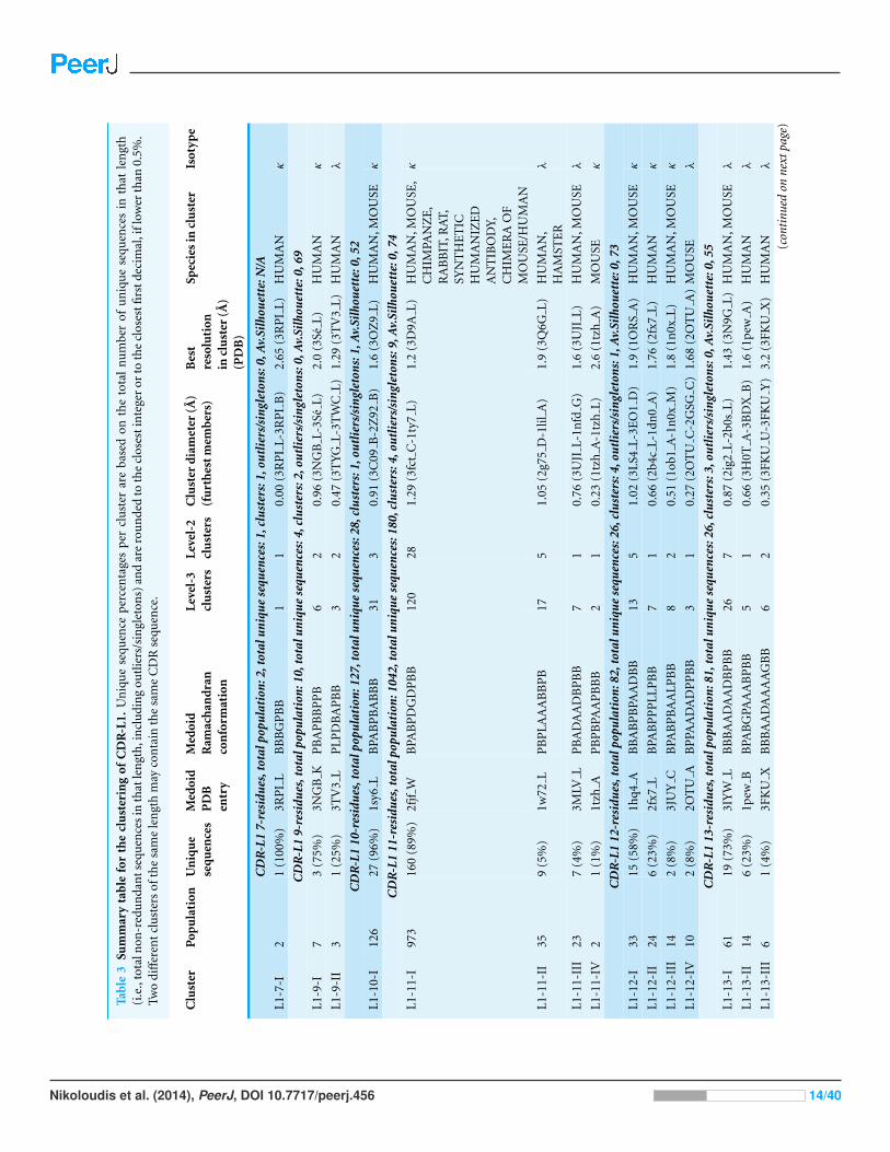
Figure 1 Superposition of 7-residue and 11-residue CDR-L2. The 5 C-terminal residues of 1A4K (inred) 7 residue CDR-L2 (L52–L56) are superposed to the equivalent portion of 3FFD (in blue) 11 residueCDR-L2. Position L51 is highlighted in green, as the best insertion point in the structural numberingscheme. Graphics created with Swiss-PdbViewer (http://www.expasy.org/spdbv/).
analysis would be more revealing and useful if the CDR-H1 extent was considered as
the entire length of the loop, namely residues H23–H35. As far as CDR-H2 was concerned,
it was observed that the C-terminal portion of Kabat’s definition (i.e., residues H59–H65)
remained relatively unchanged conformationally in most CDRs. Therefore, only the length
of the symmetrical loop portion between residues H50–H58 was retained for the CDR-H2
definition.
CDR length and numbering scheme amendmentsA number of antibodies contained a CDR with more residues than the current scheme
could accept. The CDRs concerned were CDR-L2, -L3, -H1, -H2 and -H3. These CDRs,
except for CDR-L2, already contained an insertion locus so the maximum allowed length
was extended by adding more insertion positions (letters) to the numbering scheme. An
insertion point was required in CDR-L2 for an 11-residue length. By superposing the
new 11-residue loop (PDB code 3FFD) on a typical 7-residue one (1A4K), it was strongly
suggested that the insertion point in CDR-L2 should be placed at position L51 (Fig. 1).
Two more cases required intervention in the numbering scheme. The first was in
Light chain framework-3 (LFR3), where structure 1PW3 showed a 2-residue insertion.
Superposition of this structure to the respective portion of a typical Light variable chain
(1A4K) revealed that an insertion point should be introduced at position L67 (Fig. 2).
The second case was raised by two anti-HIV antibodies observed in structures 3RPI and
3SE8, showing an insertion of 3 and 7 residues respectively in Heavy chain framework-3
(HFR3). Superposition of these frameworks onto a typical HFR3 (3MLY) suggested that
an insertion point should be placed at residue H74 (Fig. 3). Table 2 summarises all the
amendments brought to the initial numbering scheme in order to accommodate the
special cases discovered in the dataset.
Clustering overviewIn order to increase the usefulness of the clustering result in a way that meets the needs of
a wider range of applications, a novel three-level nested cluster architecture was devised.
At the parent-level, members of the same cluster share the least similarity in terms of
Nikoloudis et al. (2014), PeerJ, DOI 10.7717/peerj.456 5/40

Figure 2 Superposition of Light Framework 3 with an insertion onto a typical LFR3. Residues L60–L75of crystal structure 1PW3 (in red), containing an insertion, are superposed onto a typical example of theequivalent Light chain fragment (here 1A4K, in blue). The new insertion point was introduced in positionL67 (highlighted in green). Graphics created with Swiss-PdbViewer (http://www.expasy.org/spdbv/).
Cα-atom Root-Mean-Square Deviation (RMSD), as the cluster is designed to include all
the variants of a conformational theme within the limits of a statistical cluster validation.
At the daughter-level, RMSD variance is successively reduced and members of the same
cluster are increasingly similar. This stratified scheme could also be perceived as a variation
of sensitivity to the potential natural flexibility of a CDR conformation (looser clusters), as
well as a trade-off to the specificity of a particular shape (tighter clusters).
Nikoloudis et al. (2014), PeerJ, DOI 10.7717/peerj.456 6/40

Figure 3 Superposition of Heavy Framework 3 with an insertion onto a typical HFR3. The Cα-traceof a two-leg superposition of residues H65–H73 and H76–H78 of crystal structures 3RPI (in yellow)and 3SE8 (in red), containing an insertion, onto the equivalent residues of a typical structure withoutan insertion (here 3MLY, in blue). The proposed insertion point H74 is highlighted in green in 3MLYand is shown with its side chain (Ser). Graphics created with Swiss-PdbViewer (http://www.expasy.org/spdbv/).
First-level clusters were formed by the use of a statistical clustering method, while
second- and third-level clusters were defined using qualitative criteria. More specifically,
the data was initially analysed by average- and complete-distance hierarchical clustering
using RMSD distance matrices, and pruning of the resulting trees was performed with
the Dynamic Tree Cut algorithm (Langfelder, Zhang & Horvath, 2007). RMSD distance
matrices were obtained by performing all-by-all Cα-atom superpositions of the entire
CDR loops, per individual CDR length. The result of hierarchical clustering was a set of
level-1 structural classes, as traditionally produced by various methods in all previous CDR
conformational studies, meaning that members of the same cluster were similar to a degree
that is defined by the tree-pruning and clustering criteria.
Nikoloudis et al. (2014), PeerJ, DOI 10.7717/peerj.456 7/40

Table 2 Modifications brought to the numbering scheme. Modifications brought to the numberingscheme in the light of new and atypical sequences. LFR3, light chain framework 3; HFR3, heavy chainframework 3. CDR-H3 insertion positions H100uvw were not required in the present dataset, but wereadded for the technical continuity up to the pre-existing positions H100xyz and for future use. Thus3U1S has a CDR-H3 length of 31 residues.
Locus Numberingscheme addition
MaximumCDR length
Structures with thenew maximum length
CDRextents
CDR-L1 – 17 N/A L24-L34
CDR-L2 L51abcd 11 2GSG, 2H32, 2H3N, 2OTU,2OTW, 2QHR, 3FFD
L50-L56
LFR3 L67ab N/A 1PW3 N/A
CDR-L3 L95cd 13 2GSG, 2OTU, 2QHR, 3FFD,3MLW
L89-L97
CDR-H1 H31cdefghijk 24 3K3Q H23–H35
CDR-H2 H52ef 15 3TWC, 3TYG H50–H58
HFR3 H74abcdefg N/A 3SE8 N/A
CDR-H3 H100nopqrstuvw 34 3U1S H95-H102
Subsequently, φ/ψ angles were calculated for all CDR residues, each residue was
attributed to a Ramachandran region and Ramachandran logos were formulated for
each CDR. For practical and computational reasons, the boundaries of the different
Ramachandran regions were based on the Ramachandran Plot subdivision used by North,
Lehmann & Dunbrack (2011) (Fig. 4). Two types of Ramachandran logos are defined for
each CDR, namely one where similar conformational regions were represented by the same
letter (also suggested in North, Lehmann & Dunbrack, 2011), which will henceforth be
called the reduced-Ramachandran Logo or r-RL, and one where every conformational
region is represented individually, called the full-Ramachandran Logo or f-RL. For
the formation of level-2 clusters, the members of any given parent level-1 cluster were
regrouped by identical r-RL, meaning that members of the same cluster contain residues
at each CDR position that belong to similar conformational regions. For the formation
of level-3 clusters, the members of any given level-2 cluster were regrouped by identical
f-RL, meaning that members of the same cluster contain residues at each CDR position
that belong to the exact same conformational region. An example showing the layout of
this nested cluster architecture can be seen in Fig. 5. Outliers/singletons were all given the
tag ‘-O-‘ in their conformational logo, which created a common parent class that allowed
the subsequent formation of 2nd- and 3rd-level clusters within outlier space, as well.
Clustering methodThe RMSD distance matrices produced for each CDR/length combination were used for
hierarchical analysis in the statistical package RGui (GNU project, http://www.sciviews.
org/ rgui/). The average-linkage and complete-linkage algorithms were preferred to
single-linkage in order to avoid chaining effects in dense configurations of the dataset
in conformational space, and were both explored for every CDR/length combination.
Hierarchical trees (dendrograms) that gave a Cophenetic Correlation Coefficient (CPCC)
Nikoloudis et al. (2014), PeerJ, DOI 10.7717/peerj.456 8/40

Figure 4 Ramachandran plot divided into conformational regions. A: α-helix region; B: β-sheetregion; D: δ-region; G: γ -region; L: left-handed helix region; P: polyproline II region. For the con-struction of reduced-Ramachandran logos (r-RL), residues belonging to regions with similar confor-mations were represented by the same letter: (A/D) = A, (B/P) = B, (L/G) = L. For the constructionof full-Ramachandran logos (f-RL), each conformational region was represented individually. E.g.,Ramachandran logos for CDR-L3 1TJH L:r-RL: BBAABBBBB f-RL: BBDABPPPB.
lower than 0.6 were directly discarded as pointing to poor fitting of the data. In all
cases at least one of the hierarchical methods achieved a CPCC score greater than 0.6.
Both hierarchical trees were considered whenever the CPCC was acceptable and
comparatively evaluated using the criteria below.
The Dynamic Hybrid Tree Cut method of the Dynamic Tree Cut statistical package in
RGui was utilised for dendrogram pruning. The package has been previously successfully
used for the detection of biologically meaningful clusters in a protein–protein interaction
network in Drosophila (Dong & Horvath, 2007). The Dynamic Hybrid Tree Cut algorithm
offers flexibility, by allowing the user to set the desired pruning parameters for cluster
and outlier recognition. Specifically, the algorithm defines four cluster shape criteria:
(1) the minimum number of cluster members (N0, minClusterSize), (2) the maximum
scatter of the pairwise distances between the lowest merged objects (CDR structures) in
each cluster, called the cluster core (dmax, maxAbsCoreScatter), (3) the maximum joining
height at which a cluster attaches to the rest of the dendrogram (hmax, cutHeight), and
(4) the minimum distance between the core scatter and the joining height of a cluster to
the dendrogram, called the cluster gap (gmin, minAbsGap). The core scatter is defined as the
average of all pairwise dissimilarities between objects belonging to the core of the cluster.
Nikoloudis et al. (2014), PeerJ, DOI 10.7717/peerj.456 9/40

Figure 5 Example of the nested clusters architecture. Level-1 cluster H1-13-III (i.e., the third top-levelcluster of 13-residues CDR-H1), defined by RMSD-based hierarchical clustering, contains 3 Level-2clusters, the members of each sharing the same reduced-Ramachandran logo, and in total 11 Level-3clusters, the members of each sharing the same full-Ramachandran logo. All Level-3 clusters share thesame reduced-Ramachandran logo with their parent Level-2 cluster, but each one displays a distinctfull-Ramachandran logo.
Consequently, a branch is considered a cluster when it contains a minimum number of
members (N0), its joining height is at most hmax, its core is tightly connected (dmax) and
distinct from its neighbourhood (gmin). Specifically, the minimum cluster gap distance
(gmin) can be perceived as the minimum allowance for the cluster to expand its diameter
from its core until it reaches a neighbouring cluster.
Although these pruning parameters are explained in depth in the corresponding
method paper (Dong & Horvath, 2007), an example of the application of pruning
parameters to an actual dendrogram from this analysis can be seen in Fig. 6. The number of
objects assigned to the core of a cluster is derived from the following implemented formula:
nc = min
(N0/2 +
N − N0/2),N
(1)
with nc the number of core objects, N0 the defined minimum cluster size and N the total
number of objects in the cluster. As a consequence, the core of small clusters can be as large
as the whole cluster, while the core of large clusters remains a fraction of the lowest joined
objects.
Nikoloudis et al. (2014), PeerJ, DOI 10.7717/peerj.456 10/40

Figure 6 Illustration of the parameters taken into account for the dendrogram pruning of CDR-L1/12 residues with the Dynamic Hybrid method.The minimum gap statistic (gmin) defines the minimum required distance between the average core scatter and the joining height of the clusters(‘Gap’), for successful cluster formation. In this example, gmin is set lower than the displayed Gaps, so nodes above its value were considered asdifferent clusters.
The algorithm examines the dendrogram in a bottom-up manner and attempts to
perform three types of branch merges: a merge of two singletons which creates a new
branch, the addition of a singleton to a branch, or a merge of two branches. In each
step two branches are tested against the pruning criteria: if both considered branches
satisfy the criteria then both are declared “closed” and no further objects are added in
the current step. Otherwise, the branches are merged and this new group is reassessed for
cluster conformity during the next merge with an adjacent branch. Objects too far from a
cluster are left unlabelled as outliers. Once all possible object assignments are performed,
the method allows a further optional ‘Partitioning Around Medoids-like’ step (PAM).
During this step, unlabelled objects (outliers) are considered one-by-one and are assigned
to existing clusters based on a user-defined maximum allowable distance, or when their
distance is smaller than the cluster’s radius. There are two options available for the cluster
radius definition (parameter: useMedoids[=FALSE/TRUE]). If average distances are being
used (FALSE), then the radius of the cluster is defined as the maximum of the average
distances between objects in the cluster. If instead medoids are used (TRUE), then the
radius is defined as the maximum distance of the cluster’s medoid to the cluster’s objects.
In order to detect the pruning parameters that lead to the best clustering result, an
R routine was created which cycles the pruning method through a range of hmax, then
Nikoloudis et al. (2014), PeerJ, DOI 10.7717/peerj.456 11/40

gmin, then dmax using 0.1 increment steps. In each step, the quality of the clusters was
assessed by calculation of the average Silhouette Coefficient (SC) and a cut-off of 0.51 was
defined as the minimum required coefficient value for a reasonable structure to be found.
The minimum number of members per cluster (N0) was set to 2, in order to make sure
that true singletons that could not form a compact cluster core with sufficient separation
from neighbouring clusters were left as outliers. The output of this routine returned the
clustering parameters, the number of clusters and outliers, the average SC and an auxiliary
index showing the ratio of outliers over clusters.
Multidimensional scaling was applied to all distance matrices and 2D maps were
produced for visual inspection of the clusters. In addition, 3D maps were created and
consulted through the visualisation tool GNUPLOT (Williams et al., 2007–2011), for better
perception of the configuration of the global population of each CDR/length combination.
The 2D/3D maps and the respective Silhouette Plots of pruning results with average SC
greater than 0.51 and all positive individual Silhouette Widths (SW) were consulted in
all cases in order to continually have a visual appreciation of the data configuration and
clustering evolution, and to make informed decisions which allowed the final formalisation
of the clustering procedure. Given that the desired clustering result would ideally produce
as many well separated clusters and as few outliers as possible, the auxiliary index offered a
quick composite comparison between pruning results, and was defined as:
a = (1 + S)/C (2)
where S is the number of outliers/singletons and C the number of clusters. The unit (1) was
added to the index’s numerator in order to allow the comparison between pruning results
with 0 outliers/singletons, but a different number of clusters.
Another index employed during the clustering procedure was that of the ideal
maximum cluster diameter, which took into consideration the examined CDR length (l):
Di = 1 +
l − 9
10
. (3)
The rationale behind this formula was to define an ideal maximum diameter by adding
or subtracting 0.1 A per residue respectively above or below a length of 9. For a CDR with
9-residues, this diameter was set empirically at 1.0 A, based on experience of manual 3D
superpositions of CDR-L3/9-residues with the graphics program Swiss-PdbViewer (Spdbv;
Guex & Peitsch, 1997). Observations suggested 1.0 A to be an appropriate cut-off for
significant visual conformational similarity for CDRs of this length. This auxiliary index
played no further analytical role than to merely define a cut-off at which the possibility
of cluster splitting was to be explored during the clustering procedure. In no case did
it impose a diameter threshold for cluster formation. Conversely, cluster merging was
explored between clusters that contained one or more members with greater affinity for
the second cluster (revealed by its negative SW). If the merge resulted in a global average
SC ≥ 0.51 then it was retained, otherwise the entire partition was discarded. In the end,
the preferred clustering parameters were those that resulted in global average SC equal
Nikoloudis et al. (2014), PeerJ, DOI 10.7717/peerj.456 12/40

or higher than 0.51, all positive individual SWs and the lower auxiliary index α (Eq. (2)).
If the number of outliers remained high, the optional PAM-stage was applied at the end of
the tree cut procedure, but its results were only retained if all of the above partition quality
criteria were satisfied.
When the optimal clustering result was obtained, the clusters’ cores, medoids, most
distant members and their diameters were extracted for that CDR/length combination via
a dedicated R routine. Clustering summaries were created with Java code, as well as lists
and various post-analytical data that are detailed later.
RESULTSClustering resultsTables of results were constructed for 58 CDR/length combination, gathering information
that describes each individual cluster, which can be consulted for quick reference
(Tables 3–7 for CDR-L1/-L2/-L3/-H1/-H2 and a separate supplementary table for
CDR-H3, Supplemental Information 4). A summary table with all clustered lengths is
available in Table 8. Detailed membership assignments can be found in two forms: one
where every CDR is shown in alphabetical PDB order with all available clustering and
data-mined information (cis/trans peptides, structure resolution, crystal space group,
sequence, Ramachandran logos, cluster core label, bound state, light isotype, heavy or light
chain only) and one where the same information is given in cluster order (Supplemental
Information 6 and Supplemental Information 5). The ω-angle cut-off for cis-peptide
detection was set to ±30◦; absence of cis-content that satisfied these limits resulted in an
all-trans (allT) label. Bound state was flagged based on a list of bound antibodies obtained
from SAbDab (Dunbar et al., 2014). This list did not contain idiotype-anti-idiotype
complexes, therefore the 5 such files in the dataset were additionally flagged as bound
(entries 1CIC, 1DVF, 1IAI, 1PG7, 3BQU).
Comparison of clustering resultsThe level-1 clusters obtained in this work were compared to the clustering results
of previous major CDR studies (Tables 9–13 for CDR-L1, -L2, -L3, -H1 and -H2,
Supplemental Information 2 for CDR-H3). Specifically, comparisons were made with
the clusters found in Martin & Thornton (1996) because it was the first five CDR clustering
performed on a significant CDR dataset (57 antibody structures, 269 CDRs), presented
most major conformational classes and for these reasons is regularly cited in research of
this kind. Comparisons were also made with the clustering results in North, Lehmann
& Dunbrack (2011) as this is the most recent relevant analysis, which used the largest
CDR dataset (932 antibody structures before filtering, 1897 CDRs after filtering) until the
present study. Also included were the results from Kuroda et al. (2009) for the comparisons
in CDR-L3, as this recent dedicated analysis used an RMSD-based approach, as is the
case in this work, while using a considerable number of CDR structures (212 CDR-L3
structures). For the first five CDRs, the present study comprised 1,359 antibody structures
and 10,680 CDRs (and a total of 12,712 CDRs including CDR-H3). Commenting on these
comparisons is made in the discussion section below.
Nikoloudis et al. (2014), PeerJ, DOI 10.7717/peerj.456 13/40
Tabl
e3
Sum
mar
yta
ble
for
the
clu
ster
ing
ofC
DR
-L1.
Un
iqu
ese
quen
cep
erce
nta
ges
per
clu
ster
are
base
don
the
tota
ln
um
ber
ofu
niq
ue
sequ
ence
sin
that
len
gth
(i.e
.,to
taln
on-r
edu
nda
nts
equ
ence
sin
that
len
gth
,in
clu
din
gou
tlie
rs/s
ingl
eton
s)an
dar
ero
un
ded
toth
ecl
oses
tin
tege
ror
toth
ecl
oses
tfirs
tdec
imal
,ifl
ower
than
0.5%
.Tw
odi
ffer
ent
clu
ster
sof
the
sam
ele
ngt
hm
ayco
nta
inth
esa
me
CD
Rse
quen
ce.
Clu
ster
Pop
ula
tion
Un
iqu
ese
quen
ces
Med
oid
PD
Ben
try
Med
oid
Ram
ach
and
ran
con
form
atio
n
Leve
l-3
clu
ster
sLe
vel-
2cl
ust
ers
Clu
ster
dia
met
er(A
)(f
urt
hes
tmem
ber
s)B
est
reso
luti
onin
clu
ster
(A)
(PD
B)
Spec
ies
incl
ust
erIs
otyp
e
CD
R-L
17-
resi
dues
,tot
alpo
pula
tion
:2,t
otal
un
iqu
ese
quen
ces:
1,cl
ust
ers:
1,ou
tlie
rs/s
ingl
eton
s:0,
Av.
Silh
ouet
te:N
/A
L1-7
-I2
1(1
00%
)3R
PI
LB
BB
GP
BB
11
0.00
(3R
PI
L-3R
PI
B)
2.65
(3R
PI
L)
HU
MA
Nκ
CD
R-L
19-
resi
dues
,tot
alpo
pula
tion
:10,
tota
lun
iqu
ese
quen
ces:
4,cl
ust
ers:
2,ou
tlie
rs/s
ingl
eton
s:0,
Av.
Silh
ouet
te:0
,69
L1-9
-I7
3(7
5%)
3NG
BK
PB
AP
BB
PP
B6
20.
96(3
NG
BL-
3Se
L)2.
0(3
SeL
)H
UM
AN
κ
L1-9
-II
31
(25%
)3T
V3
LP
LPD
BA
PB
B3
20.
47(3
TY
GL-
3TW
CL)
1.29
(3T
V3
L)
HU
MA
Nλ
CD
R-L
110
-res
idu
es,t
otal
popu
lati
on:1
27,t
otal
un
iqu
ese
quen
ces:
28,c
lust
ers:
1,ou
tlie
rs/s
ingl
eton
s:1,
Av.
Silh
ouet
te:0
,52
L1-1
0-I
126
27(9
6%)
1sy6
LB
PAB
PB
AB
BB
313
0.91
(3C
09B
-2Z
92B
)1.
6(3
OZ
9L
)H
UM
AN
,MO
USE
κ
CD
R-L
111
-res
idu
es,t
otal
popu
lati
on:1
042,
tota
lun
iqu
ese
quen
ces:
180,
clu
ster
s:4,
outl
iers
/sin
glet
ons:
9,A
v.Si
lhou
ette
:0,7
4
L1-1
1-I
973
160
(89%
)2f
jfW
BPA
BP
DG
DP
BB
120
281.
29(3
fct
C-1
ty7
L)1.
2(3
D9A
L)
HU
MA
N,M
OU
SE,
CH
IMPA
NZ
E,
RA
BB
IT,R
AT,
SYN
TH
ET
ICH
UM
AN
IZE
DA
NT
IBO
DY,
CH
IME
RA
OF
MO
USE
/HU
MA
N
κ
L1-1
1-II
359
(5%
)1w
72L
PB
PLA
AA
BB
PB
175
1.05
(2g7
5D
-1lil
A)
1.9
(3Q
6GL
)H
UM
AN
,H
AM
STE
Rλ
L1-1
1-II
I23
7(4
%)
3MLV
LP
BA
DA
AD
BP
BB
71
0.76
(3U
JIL-
1nfd
G)
1.6
(3U
JIL
)H
UM
AN
,MO
USE
λ
L1-1
1-IV
21
(1%
)1t
zhA
PB
PB
PAA
PB
BB
21
0.23
(1tz
hA
-1tz
hL)
2.6
(1tz
hA
)M
OU
SEκ
CD
R-L
112
-res
idu
es,t
otal
popu
lati
on:8
2,to
talu
niq
ue
sequ
ence
s:26
,clu
ster
s:4,
outl
iers
/sin
glet
ons:
1,A
v.Si
lhou
ette
:0,7
3
L1-1
2-I
3315
(58%
)1h
q4A
BB
AB
PB
PAA
DB
B13
51.
02(3
LS4
L-3E
O1
D)
1.9
(1O
RS
A)
HU
MA
N,M
OU
SEκ
L1-1
2-II
246
(23%
)2f
x7L
BPA
BP
PP
LLP
BB
71
0.66
(2b4
cL-
1dn
0A
)1.
76(2
fx7
L)
HU
MA
Nκ
L1-1
2-II
I14
2(8
%)
3JU
YC
BPA
BP
BA
ALP
BB
82
0.51
(1ob
1A
-1n
0xM
)1.
8(1
n0x
L)
HU
MA
N,M
OU
SEκ
L1-1
2-IV
102
(8%
)2O
TU
AB
PPA
AD
AD
PP
BB
31
0.27
(2O
TU
C-2
GSG
C)
1.68
(2O
TU
A)
MO
USE
λ
CD
R-L
113
-res
idu
es,t
otal
popu
lati
on:8
1,to
talu
niq
ue
sequ
ence
s:26
,clu
ster
s:3,
outl
iers
/sin
glet
ons:
0,A
v.Si
lhou
ette
:0,5
5
L1-1
3-I
6119
(73%
)3I
YW
LB
BB
AA
DA
AD
BP
BB
267
0.87
(2ig
2L-
2b0s
L)1.
43(3
N9G
L)
HU
MA
N,M
OU
SEλ
L1-1
3-II
146
(23%
)1p
ewB
BPA
BG
PAA
AB
PB
B5
10.
66(3
H0T
A-3
BD
XB
)1.
6(1
pew
A)
HU
MA
Nλ
L1-1
3-II
I6
1(4
%)
3FK
UX
BB
BA
AD
AA
AA
GB
B6
20.
35(3
FKU
U-3
FKU
Y)
3.2
(3FK
UX
)H
UM
AN
λ
(con
tinu
edon
next
page
)
Nikoloudis et al. (2014), PeerJ, DOI 10.7717/peerj.456 14/40

Tabl
e3
(con
tinu
ed)
Clu
ster
Pop
ula
tion
Un
iqu
ese
quen
ces
Med
oid
PD
Ben
try
Med
oid
Ram
ach
and
ran
con
form
atio
n
Leve
l-3
clu
ster
sLe
vel-
2cl
ust
ers
Clu
ster
dia
met
er(A
)(f
urt
hes
tmem
ber
s)B
est
reso
luti
onin
clu
ster
(A)
(PD
B)
Spec
ies
incl
ust
erIs
otyp
e
CD
R-L
114
-res
idu
es,t
otal
popu
lati
on:2
07,t
otal
un
iqu
ese
quen
ces:
25,c
lust
ers:
7,ou
tlie
rs/s
ingl
eton
s:14
,Av.
Silh
ouet
te:0
,76
L1-1
4-I
112
10(4
0%)
1oar
LB
BA
AG
PP
BA
AA
LPB
365
1.08
(1oa
uO
-1n
j9L
)1.
5(1
oaq
L)
HU
MA
N,M
OU
SE,
RA
T,SY
NT
HE
TIC
HU
MA
NIZ
ED
AN
TIB
OD
Y
λ
L1-1
4-II
669
(36%
)3U
4EB
BB
BA
AD
AA
AB
AB
BB
5025
1.34
(1m
cwW
-1m
cqA
)1.
5(3
KD
ML)
HU
MA
N,S
EA
Lλ
L1-1
4-II
I3
1(4
%)
1lgv
BB
LAA
AP
PLA
GD
PB
B2
10.
15(1
lhz
B-1
jvk
B)
1.94
(1jv
kB
)H
UM
AN
λ
L1-1
4-IV
31
(4%
)1j
vkA
BLA
PPA
PG
BP
DP
BB
33
0.44
(1lh
zA
-1lg
vA
)1.
94(1
jvk
A)
HU
MA
Nλ
L1-1
4-V
33
(12%
)7f
abL
BB
BA
AD
AA
DLB
PB
B3
10.
36(3
H42
L-1a
qkL)
1.84
(1aq
kL
)H
UM
AN
λ
L1-1
4-V
I3
1(4
%)
2H3N
AP
PP
GA
BPA
AD
BP
BB
32
0.39
(2H
3NC
-2H
32A
)2.
3(2
H3N
A)
HU
MA
Nλ
L1-1
4-V
II3
1(4
%)
1mcs
BP
PAP
PD
PLP
BD
AP
B3
31.
18(1
mcn
B-1
mcc
B)
2.7
(1m
ccB
)H
UM
AN
λ
CD
R-L
115
-res
idu
es,t
otal
popu
lati
on:8
0,to
talu
niq
ue
sequ
ence
s:34
,clu
ster
s:2,
outl
iers
/sin
glet
ons:
48,A
v.Si
lhou
ette
:0,5
4
L1-1
5-I
2613
(38%
)2Y
5TB
BB
AB
PD
PB
LLB
PP
BB
143
0.67
(3Z
TJ
L-2n
z9C
)2.
0(1
h0d
A)
HU
MA
N,M
OU
SEκ
L1-1
5-II
63
(9%
)1i
9rL
BPA
BP
DB
BA
DB
BP
BB
41
0.61
(3P
HO
A-1
i7z
C)
2.0
(3P
HQ
A)
HU
MA
N,M
OU
SEκ
CD
R-L
116
-res
idu
es,t
otal
popu
lati
on:3
52,t
otal
un
iqu
ese
quen
ces:
74,c
lust
ers:
5,ou
tlie
rs/s
ingl
eton
s:33
,Av.
Silh
ouet
te:0
,60
L1-1
6-I
309
66(8
9%)
3QC
UL
BB
AB
PAP
PAA
LPB
PB
B81
131.
24(2
GJZ
A-1
f3d
L)1.
22(1
mju
L)
HU
MA
N,M
OU
SE,
CH
IME
RA
OF
MO
USE
/HU
MA
N
κ
L1-1
6-II
31
(1%
)1c
fvL
BPA
BP
DD
AB
AB
PLP
BB
31
0.22
(2bf
vL-
1bfv
L)2.
1(1
bfv
L)M
OU
SEκ
L1-1
6-II
I3
1(1
%)
3FO
9L
BPA
BP
DPA
BP
LBB
PB
B3
10.
36(3
FO9
A-1
axt
L)
1.9
(3FO
9L)
MO
USE
κ
L1-1
6-IV
21
(1%
)1l
7sL
BPA
BP
PP
PB
LGP
PAB
B1
10.
00(1
VP
OL-
1l7s
L)2.
15(1
l7s
L)
MO
USE
κ
L1-1
6-V
21
(1%
)1n
akL
BB
AB
PD
GB
DLD
DP
PB
B1
10.
04(1
nak
M-1
nak
L)
2.57
(1n
akL)
MO
USE
κ
CD
R-L
117
-res
idu
es,t
otal
popu
lati
on:1
72,t
otal
un
iqu
ese
quen
ces:
36,c
lust
ers:
1,ou
tlie
rs/s
ingl
eton
s:1,
Av.
Silh
ouet
te:N
/A
L1-1
7-I
171
36(1
00%
)3M
NZ
AB
BA
BP
DP
PAA
DLP
PP
BB
7117
1.51
(1xc
qG
-1h
imH
)1.
45(1
q9r
A)
HU
MA
N,M
OU
SE,
CH
IME
RA
OF
MO
USE
/HU
MA
N
κ
Tota
l(l
evel
-1cl
ust
ers
only
)
2048
533
140
Nikoloudis et al. (2014), PeerJ, DOI 10.7717/peerj.456 15/40

Tabl
e4
Sum
mar
yta
ble
for
the
clu
ster
ing
ofC
DR
-L2.
Clu
ster
Pop
ula
tion
Un
iqu
ese
quen
ces
Med
oid
PD
Ben
try
Med
oid
Ram
ach
and
ran
con
form
atio
n
Leve
l-3
clu
ster
sLe
vel-
2cl
ust
ers
Clu
ster
dia
met
er(A
)(f
urt
hes
tmem
ber
s)B
estr
esol
uti
onin
clu
ster
(A)
(PD
B)
Spec
ies
incl
ust
erIs
otyp
e
CD
R-L
27-
resi
dues
,tot
alpo
pula
tion
:216
1,to
talu
niq
ue
sequ
ence
s:27
8,cl
ust
ers:
3,ou
tlie
rs/s
ingl
eton
s:2,
Av.
Silh
ouet
te:0
,61
L2-7
-I21
0927
2(9
8%)
1dn
0C
LLD
PP
PP
121
451.
56(3
KY
MO
-1n
j9A
)1.
2(3
D9A
L)H
UM
AN
,MO
USE
,R
AB
BIT
,RA
T,SE
AL,
HA
MST
ER
,C
HIM
PAN
ZE
E,R
AT,
SYN
TH
ET
ICH
UM
AN
IZE
DA
NT
IBO
DY,
CH
IME
RA
OF
MO
USE
/HU
MA
N
κ,λ
L2-7
-II
398
(3%
)3R
IAL
GA
DB
BP
P12
51.
04(3
RH
WK
-3FK
UX
)1.
66(3
QH
FL)
HU
MA
N,M
OU
SEκ
,λ
L2-7
-III
112
(1%
)2a
6kL
LLG
GP
PD
83
0.75
(2Z
JSL-
2V7H
L)2.
5(2
a6i
A)
MO
USE
κ
CD
R-L
211
-res
idu
es,t
otal
popu
lati
on:1
3,to
talu
niq
ue
sequ
ence
s:3,
clu
ster
s:2,
outl
iers
/sin
glet
ons:
0,A
v.Si
lhou
ette
:0,9
0
L2-1
1-I
102
(67%
)2O
TU
AB
PAA
LPB
BP
PP
11
0.39
(2G
SGC
-2O
TU
C)
1.68
(2O
TU
A)
MO
USE
λ
L2-1
1-II
31
(33%
)2H
32A
BD
BA
AB
BB
PPA
32
0.2
(2H
3NC
-2H
3NA
)2.
3(2
H3N
A)
HU
MA
Nλ
Tota
l(le
vel-
1cl
ust
ers
only
)21
7214
556
Nikoloudis et al. (2014), PeerJ, DOI 10.7717/peerj.456 16/40

Tabl
e5
Sum
mar
yta
ble
for
the
clu
ster
ing
ofC
DR
-L3.
Clu
ster
Pop
ula
tion
Un
iqu
ese
quen
ces
Med
oid
PD
Ben
try
Med
oid
Ram
ach
and
ran
con
form
atio
n
Leve
l-3
clu
ster
sLe
vel-
2cl
ust
ers
Clu
ster
dia
met
er(A
)(f
urt
hes
tmem
ber
s)B
estr
esol
uti
onin
clu
ster
(A)
(PD
B)
Spec
ies
incl
ust
erIs
otyp
e
CD
R-L
35-
resi
dues
,tot
alpo
pula
tion
:10,
tota
lun
iqu
ese
quen
ces:
4,cl
ust
ers:
1,ou
tlie
rs/s
ingl
eton
s:0,
Av.
Silh
ouet
te:N
/A
L3-5
-I10
4(1
00%
)3N
GB
CB
BG
AB
21
0.26
(3U
7WL-
3Se
L)1.
9(3
SE8
L)
HU
MA
Nκ
CD
R-L
37-
resi
dues
,tot
alpo
pula
tion
:5,t
otal
un
iqu
ese
quen
ces:
2,cl
ust
ers:
1,ou
tlie
rs/s
ingl
eton
s:0,
Av.
Silh
ouet
te:N
/A
L3-7
-I5
2(1
00%
)3I
U3
LB
BD
DD
LP4
10.
49(1
mim
L-1d
fbL)
2.6
(1m
imL
)H
UM
AN
,MO
USE
κ
CD
R-L
38-
resi
dues
,tot
alpo
pula
tion
:138
,tot
alu
niq
ue
sequ
ence
s:43
,clu
ster
s:6,
outl
iers
/sin
glet
ons:
2,A
v.Si
lhou
ette
:0,5
6
L3-8
-I10
528
(65%
)1q
9wC
BP
DA
BG
BB
134
0.76
(3K
J4L-
1m71
A)
1.45
(1q9
rA
)H
UM
AN
,MO
USE
,R
AT
κ
L3-8
-II
126
(14%
)1t
zhL
BP
DB
BP
BP
95
1.18
(3D
GG
C-1
e6j
L)1.
77(2
fat
L)
HU
MA
N,M
OU
SEκ
L3-8
-III
74
(9%
)3h
flL
BP
DPA
BP
B7
40.
98(1
OR
SA
-1eh
lL)
1.7
(1Y
QV
L)
MO
USE
κ
L3-8
-IV
52
(5%
)3J
WD
LB
PD
AD
PD
P3
30.
66(2
J88
L-1r
z7L)
2.0
(1rz
7L
)H
UM
AN
,MO
USE
κ
L3-8
-V4
3(7
%)
1za3
AB
PAA
BP
DP
44
0.85
(3D
GG
A-1
za3
L)2.
3(3
DG
GA
)H
UM
AN
κ
L3-8
-VI
31
(2%
)3M
CL
LB
BA
AP
BPA
11
0.24
(3O
11A
-3O
11L)
1.7
(3M
CL
L)
CH
IME
RA
OF
MO
USE
/HU
MA
Nκ
CD
R-L
39-
resi
dues
,tot
alpo
pula
tion
:172
5,to
talu
niq
ue
sequ
ence
s:35
8,cl
ust
ers:
6,ou
tlie
rs/s
ingl
eton
s:5,
Av.
Silh
ouet
te:0
,65
L3-9
-I15
2832
8(9
2%)
1dqj
AB
BD
AB
PP
PB
153
341.
72(1
maj
A11
-1ke
lL)
1.2
(3D
9AL
)H
UM
AN
,MO
USE
,R
AT,
RA
BB
IT,
CH
IMPA
NZ
EE
,SY
NT
HE
TIC
HU
MA
NIZ
ED
AN
TIB
OD
Y,C
HIM
ER
AO
FM
OU
SE/H
UM
AN
κ
L3-9
-II
136
20(6
%)
2XZ
QL
BB
BB
GD
BP
B36
81.
36(2
E27
L-1p
w3
B)
1.5
(1oa
qL
)H
UM
AN
,MO
USE
,R
AT,
SYN
TH
ET
ICH
UM
AN
IZE
DA
NT
IBO
DY,
CH
IME
RA
OF
MO
USE
/HU
MA
N
κ,λ
L3-9
-III
408
(2%
)1o
p3L
BP
BB
AD
BB
B15
81.
4(8
fab
C-3
C08
L)1.
75(1
op3
L)
HU
MA
N,M
OU
SE,
CH
IME
RA
OF
MO
USE
/HU
MA
N
κ,λ
(con
tinu
edon
next
page
)
Nikoloudis et al. (2014), PeerJ, DOI 10.7717/peerj.456 17/40

Tabl
e5
(con
tinu
ed)
Clu
ster
Pop
ula
tion
Un
iqu
ese
quen
ces
Med
oid
PD
Ben
try
Med
oid
Ram
ach
and
ran
con
form
atio
n
Leve
l-3
clu
ster
sLe
vel-
2cl
ust
ers
Clu
ster
dia
met
er(A
)(f
urt
hes
tmem
ber
s)B
estr
esol
uti
onin
clu
ster
(A)
(PD
B)
Spec
ies
incl
ust
erIs
otyp
e
L3-9
-IV
81
(0,3
%)
3MLR
LB
BB
BB
BB
PA3
21.
24(3
MLV
M-3
MLS
M)
1.8
(3M
LR
L)
HU
MA
Nλ
L3-9
-V6
1(0
,3%
)3R
U8
LB
BB
GLL
BB
B2
20.
34(1
n0x
L-1h
zhM
)1.
8(1
n0x
L)
HU
MA
Nκ
L3-9
-VI
21
(0,3
%)
3FN
0L
BB
GB
PB
AB
A1
10.
23(3
Q1S
L-3F
N0
L)1.
8(3
FN0
L)
HU
MA
Nκ
CD
R-L
310
-res
idu
es,t
otal
popu
lati
on:1
13,t
otal
un
iqu
ese
quen
ces:
27,c
lust
ers:
12,o
utl
iers
/sin
glet
ons:
6,A
v.Si
lhou
ette
:0,5
9
L3-1
0-I
222
(7%
)3M
UG
IB
BP
BA
DLP
BB
42
0.76
(3M
UH
L-3L
RS
B)
1.8
(3U
2SL
)H
UM
AN
λ
L3-1
0-II
202
(7%
)1M
CD
AB
BP
BG
LLB
BP
159
1.28
(1m
ccA
-1lil
B)
2.0
(2m
cg2)
HU
MA
N,S
EA
Lλ
L3-1
0-II
I9
4(1
5%)
3B5G
AB
BB
PAA
LPP
B4
11.
19(3
GO
1L-
2XZ
AL)
1.36
(2X
ZC
L)
HU
MA
Nλ
L3-1
0-IV
94
(15%
)3E
YO
CB
BD
AB
BP
PP
B5
20.
51(3
F12
A-3
eyq
C)
1.8
(1jg
uL
)M
OU
SEκ
L3-1
0-V
73
(11%
)2d
d8L
BB
BB
AD
DG
PB
51
1.06
(3U
JIL-
3G6A
L)1.
6(3
UJI
L)
HU
MA
Nλ
L3-1
0-V
I5
1(4
%)
3MLY
LB
BP
BA
ALB
PB
11
0.24
(3M
LZL-
3MLY
M)
1.7
(3M
LYL
)H
UM
AN
λ
L3-1
0-V
II5
3(1
1%)
3TV
3L
BB
PB
GA
DP
BB
43
0.84
(3T
WC
L-1m
cwM
)1.
29(3
TV
3L
)H
UM
AN
λ
L3-1
0-V
III
41
(4%
)2fl
5A
BB
BPA
DLP
PB
22
0.18
(2fl
5C
-2fl
5L)
3.0
(2fl
5L
)H
UM
AN
λ
L3-1
0-IX
41
(4%
)1m
qkL
BP
DB
GB
PP
BB
31
0.31
(3H
B3
D-1
qle
L)1.
28(1
mqk
L)
MO
USE
κ
L3-1
0-X
31
(4%
)3I
DY
LB
BD
AB
BP
PB
B2
10.
23(3
IDY
C-3
IDX
L)2.
5(3
IDX
L)
HU
MA
Nκ
L3-1
0-X
I2
1(4
%)
1i7z
AB
PB
BA
BP
PB
B2
10.
12(1
i7z
A-1
i7z
C)
2.3
(1i7
zA
)C
HIM
ER
AO
FM
OU
SE/H
UM
AN
κ
L3-1
0-X
II17
3(1
1%)
1mcn
BB
BP
PPA
DB
BP
1715
1.55
(1m
chB
-1lil
A)
2.0
(2m
cg1)
HU
MA
N,S
EA
Lλ
CD
R-L
311
-res
idu
es,t
otal
popu
lati
on:1
42,t
otal
un
iqu
ese
quen
ces:
38,c
lust
ers:
9,ou
tlie
rs/s
ingl
eton
s:7,
Av.
Silh
ouet
te:0
,64
L3-1
1-I
7424
(63%
)3G
04A
BB
PB
AA
DLB
PB
272
1.72
(3M
AC
L-2r
he
A)
1.43
(3N
9GL
)H
UM
AN
,MO
USE
,H
AM
STE
Rκ
,λ
L3-1
1-II
241
(3%
)1y
ymQ
BP
DA
PB
PP
BP
B6
30.
34(1
yym
L-1g
9nL)
1.99
(2N
Y1
C)
HU
MA
Nκ
L3-1
1-II
I11
3(8
%)
2OM
NA
BB
PB
APA
BA
BB
73
1.01
(3G
HE
L-2O
MB
D)
1.5
(3K
DM
L)
HU
MA
Nλ
L3-1
1-IV
81
(3%
)2Q
R0
GB
BB
LPD
DB
AB
B8
40.
36(2
QR
0S-
2QR
0K
)3.
5(2
QR
0A
)H
UM
AN
κ
L3-1
1-V
52
(5%
)3N
H7
MB
BP
BA
PLL
BB
B4
30.
59(4
bjl
A-3
NH
7O
)2.
4(4
bjl
A)
HU
MA
Nλ
L3-1
1-V
I4
2(5
%)
2JB
6A
BB
BPA
ALD
BB
B2
10.
77(3
UJJ
L-2J
B5
L)2.
0(3
UJJ
L)
HU
MA
Nλ
L3-1
1-V
II4
1(3
%)
3EFF
CB
BD
AP
BB
LAG
B4
40.
6(3
PJS
C-3
EFF
A)
3.8
(3E
FFA
)M
OU
SEκ
L3-1
1-V
III
31
(3%
)2b
1hL
BB
PB
DA
ALB
PB
21
0.2
(2b1
aL-
2b0s
L)2.
0(2
b1h
L)
HU
MA
Nλ
L3-1
1-IX
21
(3%
)1n
fdE
BB
BB
GA
ALP
PB
11
0.17
(1n
fdE
-1n
fdG
)2.
8(1
nfd
E)
MO
USE
λ
(con
tinu
edon
next
page
)
Nikoloudis et al. (2014), PeerJ, DOI 10.7717/peerj.456 18/40

Tabl
e5
(con
tinu
ed)
Clu
ster
Pop
ula
tion
Un
iqu
ese
quen
ces
Med
oid
PD
Ben
try
Med
oid
Ram
ach
and
ran
con
form
atio
n
Leve
l-3
clu
ster
sLe
vel-
2cl
ust
ers
Clu
ster
dia
met
er(A
)(f
urt
hes
tmem
ber
s)B
estr
esol
uti
onin
clu
ster
(A)
(PD
B)
Spec
ies
incl
ust
erIs
otyp
e
CD
R-L
312
-res
idu
es,t
otal
popu
lati
on:1
9,to
talu
niq
ue
sequ
ence
s:6,
clu
ster
s:4,
outl
iers
/sin
glet
ons:
0,A
v.Si
lhou
ette
:0,7
3
L3-1
2-I
61
(17%
)2X
7LD
BB
GB
AA
GA
DG
BB
11
0.04
(2X
7LK
-2X
7LB
)3.
17(2
X7L
B)
Not
avai
labl
eκ
L3-1
2-II
61
(17%
)1q
1jL
BB
BPA
PAA
LPP
B2
10.
31(3
GH
BL-
3C2A
M)
2.1
(3C
2AL
)H
UM
AN
λ
L3-1
2-II
I4
2(3
3%)
3LZ
FL
BB
PB
AP
GA
GB
PB
33
0.9
(3Q
HZ
M-3
GB
NL)
1.55
(3Q
HZ
M)
HU
MA
Nλ
L3-1
2-IV
32
(33%
)3L
QA
LB
BP
BA
PG
AA
GP
B3
31.
35(3
P30
L-3L
MJ
L)2.
2(3
LM
JL
)H
UM
AN
λ
CD
R-L
313
-res
idu
es,t
otal
popu
lati
on:1
2,to
talu
niq
ue
sequ
ence
s:2,
clu
ster
s:3,
outl
iers
/sin
glet
ons:
1,A
v.Si
lhou
ette
:0,7
1
L3-1
3-I
61
(50%
)2O
TU
AB
BB
BP
PAA
BP
BB
B1
10.
18(2
OT
WC
-2O
TU
G)
1.68
(2O
TU
A)
MO
USE
λ
L3-1
3-II
31
(50%
)2Q
HR
LB
BB
BB
BLL
BP
BB
B3
30.
97(3
FFD
B-2
GSG
A)
2.0
(2Q
HR
L)
MO
USE
λ
L3-1
3-II
I2
1(5
0%)
3MLW
LB
BB
PD
AB
AB
PP
PB
22
0.48
(3M
LWL-
3MLW
M)
2.7
(3M
LWL
)H
UM
AN
λ
Tota
l(l
evel
-1cl
ust
ers
only
)
2143
393
153
Nikoloudis et al. (2014), PeerJ, DOI 10.7717/peerj.456 19/40

Tabl
e6
Sum
mar
yta
ble
for
the
clu
ster
ing
ofC
DR
-H1.
Leve
l-2
clu
ster
sar
esh
own
exce
ptio
nal
ly(m
arke
dw
ith
anas
teri
sk)
wh
enn
ole
vel-
1cl
ust
eris
form
ed(m
inim
um
of2
mem
bers
requ
ired
).
Clu
ster
Pop
ula
tion
Un
iqu
ese
quen
ces
Med
oid
PD
Ben
try
Med
oid
Ram
ach
and
ran
con
form
atio
n
Leve
l-3
clu
ster
sLe
vel-
2cl
ust
ers
Clu
ster
dia
met
er(A
)(f
urt
hes
tmem
ber
s)B
estr
esol
uti
onin
clu
ster
(A)
(PD
B)
Spec
ies
incl
ust
er
CD
R-H
110
-res
idu
es,t
otal
popu
lati
on:6
,tot
alu
niq
ue
sequ
ence
s:2,
clu
ster
s:1,
outl
iers
/sin
glet
ons:
0,A
v.Si
lhou
ette
:N/A
H1-
10-I
62
(100
%)
1kxq
HB
PAB
PB
AB
BB
21
0.61
(3eb
aA
-1kx
qF)
1.6
(1kx
qE
)C
AM
EL
,HU
MA
N
CD
R-H
112
-res
idu
es,t
otal
popu
lati
on:2
,tot
alu
niq
ue
sequ
ence
s:2,
clu
ster
s:0,
outl
iers
/sin
glet
ons:
2,A
v.Si
lhou
ette
:N/A
H1-
12-O
-1*
11
(50%
)1g
hf
HB
BB
BPA
AA
BP
BB
11
N/A
2.7
(1gh
fH
)M
OU
SE
H1-
12-O
-2*
11
(50%
)3I
Y2
BP
BB
LBA
BB
AB
BB
11
N/A
18.0
(3IY
2B
)M
OU
SE
CD
R-H
113
-res
idu
es,t
otal
popu
lati
on:1
845,
tota
lun
iqu
ese
quen
ces:
450,
clu
ster
s:11
,ou
tlie
rs/s
ingl
eton
s:16
4,A
v.Si
lhou
ette
:0,5
4
H1-
13-I
1555
390
(87%
)2O
SLA
PP
BLB
PAA
DB
PB
B21
423
1.74
(2G
K0
B-1
rzi
J)1.
2(3
D9A
H)
MO
USE
,HU
MA
N,
RA
T,R
AB
BIT
,L
LAM
A,H
AM
STE
R,
CH
IMPA
NZ
EE
,C
HIM
ER
AO
FM
OU
SE/H
UM
AN
,SY
NT
HE
TIC
HU
MA
NIZ
ED
AN
TIB
OD
Y
H1-
13-I
I49
6(1
%)
3F7Y
AP
BB
GP
BB
AA
PB
BB
196
1.77
(3Q
XW
D-3
GK
ZA
)1.
72(2
IH3
A)
MO
USE
,HU
MA
N,
RA
T,LL
AM
A,
CH
IME
RA
OF
MO
USE
/HU
MA
N
H1-
13-I
II24
4(1
%)
1bzq
KB
PB
LPA
BB
PAB
BB
113
1.12
(2P
42D
-1jt
pB
)1.
1(2
P45
B)
MO
USE
,D
RO
ME
DA
RY,
CA
ME
L
H1-
13-I
V8
2(0
.4%
)3Q
XV
AB
BA
BP
BA
PP
BP
BB
72
0.97
(3Q
XV
B-1
YC
7A
)1.
6(1
YC
7A
)D
RO
ME
DA
RY,
CA
ME
L
H1-
13-V
93
(1%
)2X
7LJ
PP
BLP
APA
BB
PB
B4
21.
11(2
W9E
H-1
YC
8B
)2.
7(1
YC
8B
)C
AM
EL
H1-
13-V
I9
1(0
.2%
)2W
ZP
EB
PAB
BA
BP
LPB
BB
42
0.35
(2W
ZP
J-2B
SEE
)2.
6(2
WZ
PD
)C
AM
EL
ID
H1-
13-V
II2
1(0
.2%
)1S
HM
AP
PB
GPA
AP
PB
PB
B2
10.
19(1
SHM
A-1
SHM
B)
1.9
(1SH
MA
)H
UM
AN
,MO
USE
,L
LAM
A
H1-
13-V
III
85
(1%
)3E
ZJ
BB
PB
GPA
AA
PD
BB
B6
21.
05(1
zvy
A-1
SJX
A)
1.5
(1zv
hA
)H
UM
AN
,CA
ME
L,
LLA
MA
H1-
13-I
X3
1(0
.2%
)3G
BM
HB
BP
GG
AP
BD
BP
BB
31
0.17
(3G
BN
H-3
GB
MI)
2.2
(3G
BN
H)
HU
MA
N
H1-
13-X
31
(0.2
%)
2X89
AB
BB
LPP
LLB
BP
BB
21
0.22
(2X
89C
-2X
89B
)2.
16(2
X89
A)
HU
MA
N
H1-
13-X
I2
1(0
.2%
)1n
gxB
PPA
LPP
BA
BB
PB
B1
10.
01(1
ngx
H-1
ngx
B)
1.8
(1n
gxB
)H
UM
AN
,MO
USE
CD
R-H
114
-res
idu
es,t
otal
popu
lati
on:7
2,to
talu
niq
ue
sequ
ence
s:17
,clu
ster
s:1,
outl
iers
/sin
glet
ons:
2,A
v.Si
lhou
ette
:0,6
4
H1-
14-I
7016
(94%
)1k
cvH
BB
BLB
PAA
AB
GB
BB
4711
1.37
(2f5
8H
-2aj
zH
)1.
3(1
ncw
H)
HU
MA
N,M
OU
SE(c
onti
nued
onne
xtpa
ge)
Nikoloudis et al. (2014), PeerJ, DOI 10.7717/peerj.456 20/40

Tabl
e6
(con
tinu
ed)
Clu
ster
Pop
ula
tion
Un
iqu
ese
quen
ces
Med
oid
PD
Ben
try
Med
oid
Ram
ach
and
ran
con
form
atio
n
Leve
l-3
clu
ster
sLe
vel-
2cl
ust
ers
Clu
ster
dia
met
er(A
)(f
urt
hes
tmem
ber
s)B
estr
esol
uti
onin
clu
ster
(A)
(PD
B)
Spec
ies
incl
ust
er
CD
R-H
115
-res
idu
es,t
otal
popu
lati
on:1
28,t
otal
un
iqu
ese
quen
ces:
29,c
lust
ers:
3,ou
tlie
rs/s
ingl
eton
s:3,
Av.
Silh
ouet
te:0
,62
H1-
15-I
117
25(8
6%)
2HW
ZH
BB
BLB
BA
AP
PLP
BB
B43
121.
68(3
BQ
UB
-3B
2VH
)1.
5(3
IFL
H)
HU
MA
N,M
OU
SE
H1-
15-I
I6
2(7
%)
3BA
EH
BB
BLB
BA
AA
ALP
PB
B4
20.
86(3
BK
CH
-3A
AZ
A)
1.59
(3B
AE
H)
HU
MA
N,M
OU
SE
H1-
15-I
II2
1(3
%)
3FZ
UH
BB
BLP
AP
PAA
DB
PB
B2
10.
28(3
FZU
C-3
FZU
H)
2.5
(3FZ
UH
)H
UM
AN
CD
R-H
116
-res
idu
es,t
otal
popu
lati
on:3
,tot
alu
niq
ue
sequ
ence
s:2,
clu
ster
s:1,
outl
iers
/sin
glet
ons:
1,A
v.Si
lhou
ette
:N/A
H1-
16-I
21
(50%
)3e
akB
PB
BG
LAA
BPA
AA
PP
BB
11
0.42
(3ea
kA
-3ea
kB
)1.
95(3
eak
A)
CA
ME
L
CD
R-H
124
-res
idu
es,t
otal
popu
lati
on:1
,tot
alu
niq
ue
sequ
ence
s:1,
clu
ster
s:0,
outl
iers
/sin
glet
ons:
1,A
v.Si
lhou
ette
:N/A
H1-
24-O
-1*
11
(100
%)
3K3Q
AP
PB
LBA
LDLG
AA
GA
AD
AA
DB
GB
BB
11
N/A
2.6
(3K
3QA
)L
LAM
A
Tota
l(l
evel
-1cl
ust
ers
only
)
1884
379
77
Nikoloudis et al. (2014), PeerJ, DOI 10.7717/peerj.456 21/40

Tabl
e7
Sum
mar
yta
ble
for
the
clu
ster
ing
ofC
DR
-H2.
Leve
l-2
clu
ster
sar
esh
own
exce
ptio
nal
ly(m
arke
dw
ith
anas
teri
sk)
wh
enn
ole
vel-
1cl
ust
eris
form
ed(m
inim
um
of2
mem
bers
requ
ired
).
Clu
ster
Pop
ula
tion
Un
iqu
ese
quen
ces
Med
oid
PD
Ben
try
Med
oid
Ram
ach
and
ran
con
form
atio
n
Leve
l-3
clu
ster
sLe
vel-
2cl
ust
ers
Clu
ster
dia
met
er(A
)(f
urt
hes
tmem
ber
s)B
estr
esol
uti
onin
clu
ster
(A)
(PD
B)
Spec
ies
incl
ust
er
CD
R-H
28-
resi
dues
,tot
alpo
pula
tion
:6,t
otal
un
iqu
ese
quen
ces:
2,cl
ust
ers:
1,ou
tlie
rs/s
ingl
eton
s:0,
Av.
Silh
ouet
te:N
/A
H2-
8-I
62
(100
%)
1f2x
KB
BB
GA
PB
B3
31.
00(2
OJZ
H-1
f2x
K)
1.89
(2O
K0
H)
CA
ME
L,M
OU
SE
CD
R-H
29-
resi
dues
,tot
alpo
pula
tion
:436
,tot
alu
niq
ue
sequ
ence
s:11
7,cl
ust
ers:
6,ou
tlie
rs/s
ingl
eton
s:1,
Av.
Silh
ouet
te:0
,68
H2-
9-I
412
110
(94%
)1f
e8I
BB
PAA
LPB
B31
91.
47(3
K81
B-2
aj3
B)
1.2
(3D
9AH
)H
UM
AN
,MO
USE
,R
AT,
CA
ME
L,L
LAM
A,
CH
IME
RA
OF
MO
USE
/HU
MA
N,
HA
MST
ER
,AL
PAC
A,
RA
BB
IT
H2-
9-II
113
(3%
)2a
k1H
BB
BLL
DB
BB
32
1.03
(2aj
uH
-1m
coH
)1.
5(2
aju
H)
HU
MA
N,M
OU
SE
H2-
9-II
I4
1(1
%)
3UA
JH
BB
BA
DP
PP
B2
10.
14(3
UC
0H
-3U
AJ
H)
2.71
(3U
C0
H)
CH
IMPA
NZ
EE
H2-
9-IV
42
(2%
)1k
enH
BLP
AA
GA
AG
44
1.46
(1ke
nT
-1bg
xH
)2.
2(1
ay1
H)
MO
USE
H2-
9-V
21
(1%
)1Y
C7
AB
BB
PP
LPB
B1
10.
13(1
YC
7A
-1Y
C7
B)
1.6
(1Y
C7
A)
CA
ME
L
H2-
9-V
I2
1(1
%)
2aj3
DB
BB
AB
GP
BB
11
0.19
(2aj
3D
-2aj
3F)
2.03
(2aj
3D
)H
UM
AN
CD
R-H
210
-res
idu
es,t
otal
popu
lati
on:1
508,
tota
lun
iqu
ese
quen
ces:
381,
clu
ster
s:10
,ou
tlie
rs/s
ingl
eton
s:15
2,A
v.Si
lhou
ette
:0,5
6
H2-
10-I
822
238
(62%
)1u
ywH
BB
PAA
ALP
BB
6216
1.40
(1rz
iJ-
1a5f
H)
1.22
(1m
juH
)H
UM
AN
,MO
USE
,L
LAM
A,C
AM
EL
,R
AT,
SYN
TH
ET
ICH
UM
AN
IZE
DA
NT
IBO
DY
H2-
10-I
I41
710
1(2
7%)
1i8i
BB
BPA
ALA
BB
B48
181.
46(3
GJE
H-1
R24
B)
1.06
(2X
1QA
)H
UM
AN
,MO
USE
,L
LAM
A,C
AM
EL
H2-
10-I
II75
1(0
.3%
)2K
H2
B20
BB
PAA
LDP
BP
356
1.31
(2K
H2
B50
-2K
H2
B17
)N
/AM
OU
SE
H2-
10-I
V19
1(0
.3%
)1v
hp
A11
BB
PG
ALA
PB
B3
20.
88(1
vhp
A5-
1vh
pA
6)N
/AH
UM
AN
H2-
10-V
72
(1%
)1G
9EA
BB
PB
DLD
BP
B7
31.
19(1
G9E
9-1d
6vH
)2.
0(1
d6v
H)
LLA
MA
,C
HIM
ER
AO
FM
OU
SE/H
UM
AN
H2-
10-V
I4
1(0
.3%
)1b
zqM
BB
PAPA
BB
PB
11
0.03
(1bz
qL-
1bzq
N)
2.8
(1bz
qK
)D
RO
ME
DA
RY
H2-
10-V
II4
2(1
%)
1cfv
HB
BPA
ALB
PD
B2
20.
86(1
zv5
A-1
bfv
H)
2.0
(1zv
5A
)M
OU
SE,C
AM
EL
H2-
10-V
III
31
(0.3
%)
2fd6
HB
BB
GB
AA
BB
B2
20.
89(3
BT
2H
-2fa
tH
)1.
77(2
fat
H)
MO
USE
H2-
10-I
X3
2(1
%)
2fjg
BB
PB
AP
LLP
PB
32
0.97
(3LM
JH
-2fj
gH
)2.
2(3
LM
JH
)H
UM
AN
H2-
10-X
21
(0.3
%)
3NC
YQ
BB
PAA
DP
BB
B1
10.
00(3
NC
YQ
-3N
CY
P)
3.2
(3N
CY
Q)
MO
USE
(con
tinu
edon
next
page
)
Nikoloudis et al. (2014), PeerJ, DOI 10.7717/peerj.456 22/40

Tabl
e7
(con
tinu
ed)
Clu
ster
Pop
ula
tion
Un
iqu
ese
quen
ces
Med
oid
PD
Ben
try
Med
oid
Ram
ach
and
ran
con
form
atio
n
Leve
l-3
clu
ster
sLe
vel-
2cl
ust
ers
Clu
ster
dia
met
er(A
)(f
urt
hes
tmem
ber
s)B
estr
esol
uti
onin
clu
ster
(A)
(PD
B)
Spec
ies
incl
ust
er
CD
R-H
211
-res
idu
es,t
otal
popu
lati
on:3
,tot
alu
niq
ue
sequ
ence
s:3,
clu
ster
s:0,
outl
iers
/sin
glet
ons:
3,A
v.Si
lhou
ette
:N/A
H2-
11-O
-1-1
*1
1(3
3%)
2X6M
AB
BP
PLL
PD
PB
B1
1N
/A1.
62(2
X6M
A)
DR
OM
ED
AR
Y
H2-
11-O
-2-1
*1
1(3
3%)
3SE
9H
BB
PAA
DLP
BB
B1
1N
/A2.
0(3
SE9
H)
HU
MA
N
H2-
11-O
-3-1
*1
1(3
3%)
3H0T
BB
BB
BB
LBP
BB
B1
1N
/A1.
89(3
H0T
B)
HU
MA
N
CD
R-H
212
-res
idu
es,t
otal
popu
lati
on:1
71,t
otal
un
iqu
ese
quen
ces:
38,c
lust
ers:
4,ou
tlie
rs/s
ingl
eton
s:0,
Av.
Silh
ouet
te:0
,78
H2-
12-I
160
36(9
5%)
3IJH
BB
BP
PAA
ALL
PB
B19
71.
62(4
fab
H-2
aeq
H)
1.45
(1d
lfH
)H
UM
AN
,MO
USE
,R
AT,
CH
IME
RA
OF
MO
USE
/HU
MA
N
H2-
12-I
I4
1(3
%)
1aif
HB
PB
DA
LPA
BB
BB
22
1.32
(1ia
iI-
1aif
H)
2.9
(1ai
fH
)M
OU
SE
H2-
12-I
II4
1(3
%)
3IX
XG
Not
avai
labl
e1
10.
1(3
IXX
I-3I
XY
G)
15.0
(3IX
XG
)M
OU
SE
H2-
12-I
V3
1(3
%)
3QH
ZI
BB
PAA
PAP
BB
BP
22
0.4
(3Q
HZ
H-3
LZF
H)
1.55
(3Q
HZ
H)
HU
MA
N
CD
R-H
215
-res
idu
es,t
otal
popu
lati
on:6
,tot
alu
niq
ue
sequ
ence
s:3,
clu
ster
s:2,
outl
iers
/sin
glet
ons:
1,A
v.Si
lhou
ette
:0,8
4
H2-
15-I
31
(33%
)1i
3vB
BB
PD
BPA
BA
DB
PP
31
0.55
(1i3
vA
-1i3
uA
)1.
95(1
i3u
A)
LLA
MA
H2-
15-I
I2
1(3
3%)
3TY
GH
BB
BA
PB
BA
DB
DG
BB
B2
10.
29(3
TY
GH
-3T
V3
H)
1.29
(3T
V3
H)
HU
MA
N
Tota
l(l
evel
-1cl
ust
ers
only
)
1973
238
88
Nikoloudis et al. (2014), PeerJ, DOI 10.7717/peerj.456 23/40

Table 8 Summation of clustered lengths per CDR. (A) Summation of clustered lengths per CDR, with population, non-redundant sequences,number of clusters and outliers information. CDR lengths that were clustered for the first time are highlighted in bold/italics. (B) The completeCDR-H3 conformation, using the H95-H102 extents definition, has not been extensively clustered before; therefore only lengths that were notconsidered in Kuroda et al. (2009) are noted as new for conformity with the literature. CDR-H3 lengths 4 and 24 are marked with an asterisk as thecorresponding structures are also found in North, Lehmann & Dunbrack (2011), but acknowledged as 2 residues longer, due to different CDR-H3extents (H93-H102).
(A)
CDR Observed lengths(new lengths)
Total structurepopulation
Uniquesequences
Level-1clusters
Level-1 onlystructure population
Singletons/outliers
7 2 1 1 2 0
9 10 4 2 10 0
10 127 28 1 126 1
11 1,042 180 4 1,033 9
12 82 26 4 81 1
13 81 26 3 81 0
14 207 25 7 193 14
15 80 34 2 32 48
16 352 74 5 319 33
L1
17 172 36 1 171 1
Total 10 lengths 2,155 434 30 2,048 107
CDR Observed lengths Total structurepopulation
Uniquesequences
Level-1clusters
Level-1 onlystructure population
Singletons/outliers
7 2,161 278 3 2,159 2L2
11 13 3 2 13 0
Total 2 lengths 2,174 281 5 2,172 2
CDR Observed lengths(new lengths)
Total structurepopulation
Uniquesequences
Level-1clusters
Level-1 onlystructure population
Singletons/outliers
5 10 4 1 10 0
7 5 2 1 5 0
8 138 43 6 136 2
9 1,725 358 6 1,720 5
10 113 27 12 107 6
11 142 38 9 135 7
12 19 6 4 19 0
L3
13 12 2 3 11 1
Total 8 lengths 2,164 480 42 2,143 21
CDR Observed lengths(new lengths)
Total structurepopulation
Uniquesequences
Level-1clusters
Level-1 onlystructure population
Singletons/outliers
10 6 2 1 6 0
12 2 2 0 0 2
13 1,845 450 11 1,681 164
14 72 17 1 70 2
15 128 29 3 125 3
16 3 2 1 2 1
H1
24 1 1 0 0 1
Total 7 lengths 2,057 503 17 1,884 173
(continued on next page)
Nikoloudis et al. (2014), PeerJ, DOI 10.7717/peerj.456 24/40

Table 8 (continued)
(B)
CDR Observed lengths(new lengths)
Structurepopulation
Uniquesequences
Level-1clusters
Level-1 onlystructure population
Singletons/outliers
8 6 2 1 6 0
9 436 117 6 435 1
10 1,508 381 10 1,356 152
11 3 3 0 0 3
12 171 38 4 171 0
H2
15 6 3 2 5 1
Total 6 lengths 2,130 544 23 1,973 157
CDR Observed lengths(new lengths)
Structurepopulation
Uniquesequences
Level-1clusters
Level-1 onlystructure population
Singletons/outliers
3 18 4 1 18 0
4* 38 12 2 36 2
5 93 28 6 85 8
6 33 12 3 30 3
7 97 41 7 69 28
8 168 46 7 141 27
9 181 55 8 132 49
10 377 98 35 292 85
11 231 64 26 151 80
12 206 51 21 174 32
13 130 42 22 105 25
14 128 40 19 104 24
15 96 23 18 81 15
16 40 16 8 28 12
17 28 14 6 19 9
18 37 11 6 31 6
19 48 12 9 46 2
20 13 4 3 13 0
21 10 1 1 10 0
22 33 4 2 31 2
23 1 1 0 0 1
24* 12 2 2 12 0
25 1 1 0 0 1
28 12 2 1 12 0
H3
31 1 1 0 0 1
Total 25 lengths 2,032 585 213 1,620 412
Cumulativetotal(all CDRs)
58 lengths 12,712 2,827 330 11,840 872
Nikoloudis et al. (2014), PeerJ, DOI 10.7717/peerj.456 25/40

Table 9 Comparison of level-1 conformational clusters obtained in CDR-L1 with external sets. Thecluster medoid/median or representative of the external sets was used for identification of correspon-dences. In brackets, next to each correspondence, is the full, 3-level classification in this work of therepresentative of the external set and the number of corresponding members in full population compar-ison. Martin & Thornton (1996) cluster 14F is marked with a question mark, because its representative(2BJL, superseded by 4BJL) actually has a 13-residue CDR-L1.
This work[CDR-L1 cluster]
Martin & Thornton, 1996⟨corresponding cluster/canonical⟩(level-3 of external median)(corresponding members)
North, Lehmann & Dunbrack, 2011⟨corresponding cluster⟩(level-3 of external median)(corresponding members)
L1-7-I – –
L1-9-I – –
L1-9-II – –
L1-10-I 10A/1 (L1-10-I-1-1) (4/4) L1-10-1 (L1-10-I-1-1) (20/20)L1-10-2 (L1-10-I-2-2) (2/2)
L1-11-I 11A/2 (L1-11-I-2-1) (22/22) L1-11-1 (L1-11-I-1-2) (76/76)L1-11-2 (L1-11-I-2-1) (55/55)
L1-11-II – L1-11-3 (L1-11-II-1-2) (3/5)
L1-11-III 11B/- (L1-11-III-1-1) (1/1) –
L1-11-IV – –
L1-12-I – L1-12-1 (L1-12-I-1-1) (5/5)
L1-12-II – L1-12-2 (L1-12-II-1-2) (4/5)
L1-12-III – –
L1-12-IV – L1-12-3 (L1-12-IV-1-2) (2/2)
L1-13-I 13A/5λ(L1-13-I-1-2) (2/2)14F/-?(L1-13-I-7-1) (1/1)
L1-13-1 (L1-13-I-1-2) (7/7)
L1-13-II – L1-13-2 (L1-13-II-1-1) (4/4)
L1-13-III – –
L1-14-I 14B/7λ(L1-14-I-2-3) (3/3) L1-14-1 (L1-14-I-1-3) (14/14)
L1-14-II 14C/- (L1-14-II-13-1) (1/1)14E/-(L1-14-II-14-1) (1/1)
L1-14-2 (L1-14-II-4-1) (3/4)
L1-14-III – –
L1-14-IV – –
L1-14-V 14A/6λ(L1-14-V-1-2) (1/1) –
L1-14-VI – –
L1-14-VII – –
L1-15-I – L1-15-1 (L1-15-I-1-11) (8/11)
L1-15-II – –
L1-16-I 16A/4 (L1-16-I-1-51) (8/9)16C/-(L1-16-I-1-20) (1/1)
L1-16-1 (L1-16-I-1-1) (62/68)
L1-16-II – –
L1-16-III – –
L1-16-IV – –
L1-16-V – –
L1-17-I 17A/3 (L1-17-I-1-17) (4/4) L1-17-1 (L1-17-I-1-3) (21/21)
(continued on next page)
Nikoloudis et al. (2014), PeerJ, DOI 10.7717/peerj.456 26/40

Table 9 (continued)This work[CDR-L1 cluster]
Martin & Thornton, 1996⟨corresponding cluster/canonical⟩(level-3 of external median)(corresponding members)
North, Lehmann & Dunbrack, 2011⟨corresponding cluster⟩(level-3 of external median)(corresponding members)
Outliers
L1-12-O 12A/6 (L1-12-O-1-1) (1/1) –
L1-14-O 14D/- (L1-14-O-3-1) (1/1) –
L1-15-O 15A/5 (L1-15-O-6-1) (1/1)15B/- (L1-15-O-1-4) (2/2)
L1-15-2 (L1-15-O-3-1) (2/2)
L1-16-O 16B/- (L1-16-O-8-1) (2/2) –
Table 10 Comparison of level-1 conformational clusters obtained in CDR-L2 with external sets. Seenotes in Table 9. In North, Lehmann & Dunbrack (2011), the CDR extents were defined as L49-L56,instead of L50-L56; hence a direct comparison is not possible. Nonetheless, since position L49 is fairlyconserved structurally and for reference reasons, a correspondence of the longer by 1 residue clusters isshown, based on the representative of those clusters (in square brackets and in full-italics).
This work[CDR-L2 cluster]
Martin & Thornton, 1996⟨corresponding cluster/canonical⟩(level-3 of external median)(corresponding members)
North, Lehmann & Dunbrack, 2011⟨corresponding cluster⟩(level-3 of external median)(corresponding members)
L2-7-I 7A/1 (L2-7-I-2-1) (55/55) [L2-8-1 (L2-7-I-2-1) (290/290)L2-8-2 (L2-7-I-6-2) (9/9)L2-8-4 (L2-7-I-10-1) (2/2)L2-8-5 (L2-7-I-14-2) (2/2)]
L2-7-II – [L2-8-3 (L2-7-II-1-2) (3/3)]
L2-7-III 7B/1 (L2-7-III-1-6) (1/1) –
L2-11-I – [L2-12-2 (L2-11-I-1-1) (2/2)]
L2-11-II – [L2-12-1 (L2-11-II-2-1) (2/2)]
Rogue clusters and sequencesAssigned as ‘rogue’ were two conformational clusters that contain one or more members
with identical CDR sequences. This definition was first used for CDR conformations by
Martin & Thornton (1996) with respect to their unpredictability by canonical sequence
templates when all their key residues are overlapping. In this work there is an expansion
of this notion with the term ‘rogue CDR sequences’. This refers specifically to those
identical sequences that are found to exist with more than one distinct conformation.
The extraction of such sequences allows for further investigation, which can reveal any
particular circumstances or neighbouring sequence features that led to a different CDR
conformation despite the identical sequence. For example, examination of antibody Fvs
with rogue CDR sequences may reveal the influence of neighbouring main-chain atoms, a
particular framework residue influencing the CDR conformation, a conformational switch
due to interface interactions (e.g., with an antigen), intrusive crystal-packing interactions,
or even suggest some experimental error.
Nikoloudis et al. (2014), PeerJ, DOI 10.7717/peerj.456 27/40

Table 11 Comparison of level-1 conformational clusters obtained in CDR-L3, with external sets. See notes in Table 9. In Kuroda et al. (2009),no cluster representatives are available, so the cluster member with the best resolution was arbitrarily selected in each case, in order to identify thecorrespondences with the results from the present study.
This work[CDR-L3 cluster]
Martin & Thornton, 1996⟨corresponding cluster/canonical⟩(level-3 of external median)(corresponding members)
North, Lehmann & Dunbrack, 2011⟨corresponding cluster⟩(level-3 of external median)(corresponding members)
Kuroda et al., 2009⟨corresponding cluster⟩(representative)(level-3 of external representative)(corresponding members)
L3-5-I – – –
L3-7-I 7A/4 (L3-7-I-1-2) (1/1) L3-7-1(L3-7-I-1-2) (2/2)
4(1MIM)(L3-7-I-1-1) (1/1)
L3-8-I 8B/- (L3-8-I-1-1) (1/1) L3-8-1(L3-8-I-1-1) (14/15)
3B(1PZ5)(L3-8-I-2-1) (4/4)6(1Q9W)(L3-8-I-1-1) (6/6)
L3-8-II L3-8-cis6-1(L3-8-II-2-1) (3/3)
7(2FAT)(L3-8-II-2-1) (2/2)
L3-8-III 8A/3 (L3-8-III-1-1) (1/1) L3-8-2(L3-8-III-2-1) (3/4)
3A(1YQV)(L3-8-III-1-1) (2/2)
L3-8-IV – – –
L3-8-V – – –
L3-8-VI – – –
L3-9-I 9A/1 (L3-9-I-1-1) (40/40) L3-9-cis7-1(L3-9-I-1-1) (219/219)L3-9-2(L3-9-I-9-1) (12/12)L3-9-cis7-2(L3-9-I-15-2) (8/8)L3-9-cis7-3(L3-9-I-12-4) (2/2)
1(1MJU)(L3-9-I-1-2) (159/161)
L3-9-II 9C/4λ (L3-9-II-1-8) (2/2)9D/- (L3-9-II-1-4) (2/2)9E/1 (L3-9-II-5-1) (1/1)
L3-9-1(L3-9-II-2-1) (17/22)
1A (1A6V)(L3-9-II-1-4) (5/5)1B (7FAB)(L3-9-II-1-8) (1/1)1C (1Q0X)(L3-9-II-2-2) (2/2)
L3-9-III 9B/2 (L3-9-III-1-1) (1/1)9F/- (L3-9-III-7-1) (1/1)
L3-9-cis6-1(L3-9-III-1-1) (1/1)
(9-)2 (2FBJ)(L3-9-III-1-1) (1/1)
L3-9-IV – – –
L3-9-V – – –
L3-9-VI – – –
L3-10-I – – –
L3-10-II – – –
L3-10-III – L3-10-1 (L3-10-III-1-2) (2/6) –
L3-10-IV – L3-10-cis7,8-1 (L3-10-IV-1-2) (1/1) 5(1JGU) (L3-10-IV-1-2) (1/1)
L3-10-V – – –
L3-10-VI – – –
L3-10-VII 10B/-(L3-10-VII-3-1) (1/1) – –(continued on next page)
Nikoloudis et al. (2014), PeerJ, DOI 10.7717/peerj.456 28/40
Table 11 (continued)This work[CDR-L3 cluster]
Martin & Thornton, 1996⟨corresponding cluster/canonical⟩(level-3 of external median)(corresponding members)
North, Lehmann & Dunbrack, 2011⟨corresponding cluster⟩(level-3 of external median)(corresponding members)
Kuroda et al., 2009⟨corresponding cluster⟩(representative)(level-3 of external representative)(corresponding members)
L3-10-VIII – – –
L3-10-IX – – –
L3-10-X – – –
L3-10-XI – L3-10-cis8-1 (L3-10-XI-1-2) (1/2) –
L3-10-XII 10C/- (L3-10-XII-3-1) (1/1)10D/- (L3-10-XII-8-1) (1/1)
– –
L3-11-I 11A/5λ (L3-11-I-1-1) (2/2) L3-11-1 (L3-11-I-1-2) (8/9) (11-)2 (2FB4) (L3-11-I-1-1) (3/5)
L3-11-II – L3-11-cis7-1 (L3-11-II-1-2) (1/1) 8(2NY1) (L3-11-II-1-2) (1/1)
L3-11-III – – –
L3-11-IV – – –
L3-11-V 11B/- (L3-11-V-1-1) (1/1) – –
L3-11-VI – – –
L3-11-VII – – –
L3-11-VIII – – –
L3-11-IX – – –
L3-12-I – – –
L3-12-II – L3-12-1 (L3-12-II-1-1) (1/1) –
L3-12-III – – –
L3-12-IV – – –
L3-13-I – L3-13-1 (L3-13-I-1-1) (1/3) –
L3-13-II – – –
L3-13-III – – –
Outliers
L3-10-O 10A/5 (L3-10-O-6-1) (1/1) – –
All cluster populations were parsed for rogue CDR sequences and a list of CDRs,
tagged by their cluster assignment, was created for future detailed analysis (Supplemental
Information 1). Also in the same file, entries with completely identical Fvs which belong
to different conformational clusters (full-chain rogues) are reported separately, while
entries containing bound antibodies are flagged as such by an asterisk. Furthermore,
cluster populations were compared in all CDR/length sets, and the minimum number of
amino acid differences, position-by-position, was calculated between any two sequences of
different clusters. This difference was termed the ‘minimum pairwise Sequence Distance
between clusters’, or mSD (essentially a minimum Hamming distance between sequences).
Matrices showing the mSD between all clusters were constructed for every CDR/length,
and heatmaps were produced in order to allow a quick visual appreciation of the degree
of sequence dissimilarity between clusters (Supplemental Information 3). The purpose
of these heatmaps is to assist mutation studies by promptly directing the researcher to
clusters/CDR sequences of interest, as well as sequence-to-structure studies by biologists or
modellers.
Nikoloudis et al. (2014), PeerJ, DOI 10.7717/peerj.456 29/40

Table 12 Comparison of level-1 conformational clusters obtained in CDR-H1 with external sets. Seenotes in Table 9. In Martin & Thornton (1996), the CDR extents definition is significantly different(H26-H35), but correspondences based on median structures are shown for reference (in square bracketsand full-italics).
This work[CDR-H1 cluster]
Martin & Thornton, 1996⟨corresponding cluster/canonical⟩(level-3 of external median)(corresponding members)
North, Lehmann & Dunbrack, 2011⟨corresponding cluster⟩(level-3 of external median)(corresponding members)
H1-10-I – H1-10-1 (H1-10-I-1-2) (2/2)
H1-13-I [10A/1 (H1-13-I-1-2) (43/44)] H1-13-1 (H1-13-I-1-1) (261/267)H1-13-2 (H1-13-I-13-4) (2/7)H1-13-4 (H1-13-I-2-19) (3/4)H1-13-7 (H1-13-I-8-4) (3/3)
H1-13-II – H1-13-8 (H1-13-II-4-1) (2/3)
H1-13-III – H1-13-6 (H1-13-III-1-2) (2/4)H1-13-cis9-1 (H1-13-III-2-4) (2/2)
H1-13-IV – –
H1-13-V – –
H1-13-VI – –
H1-13-VII – –
H1-13-VIII – H1-13-5 (H1-13-VIII-1-5) (4/4)
H1-13-IX – –
H1-13-X – –
H1-13-XI – –
H1-14-I [11A/2 (H1-14-I-11-1) (1/1)] H1-14-1 (H1-14-I-3-11) (11/11)
H1-15-I [12A/3 (H1-15-I-2-7) (1/1)] H1-15-1 (H1-15-I-2-3) (9/9)
H1-15-II – –
H1-15-III – –
H1-16-I – –
Outliers
H1-12-O – H1-12-1 (H1-12-O-1-1) (1/1)
H1-13-O [10B/1 (H1-13-O-66-1) (1/1)10C/1 (H1-13-O-20-3) (1/1)10D (H1-13-O-31-1) (1/1)]
H1-13-3 (H1-13-O-14-1) (5/5)H1-13-9 (H1-13-O-57-1) (1/3)H1-13-10 (H1-13-O-34-1) (2/2)H1-13-11 (H1-13-O-56-1) (1/2)
H1-16-O – H1-16-1 (H1-16-O-1-1) (1/1)
H1-24-O – –
Investigation of structure resolution in outlier spaceAs a preliminary layer of quality assessment for the outliers in the present clustering,
the min, max, average and median resolutions were calculated in clustered and outlier
spaces per CDR/length (-L1, -L3, -H1, -H2, being of the highest interest). These values
were plotted as stock charts for comparison, in order to observe any global correlation
between the outlier space content and possibly erroneous CDR structures due to poor
resolution (Supplemental Information 7). In only four cases (CDR-H1/15-, CDR-H1/16-,
CDR-L1/12- and CDR-L1/16-residues) was the median resolution of outlier space found
Nikoloudis et al. (2014), PeerJ, DOI 10.7717/peerj.456 30/40

Table 13 Comparison of level-1 conformational clusters obtained in CDR-H2, with external sets. Seenotes in Table 9.
This work[CDR-H2 cluster]
Martin & Thornton, 1996⟨corresponding cluster/canonical⟩(level-3 of external median)(corresponding members)
North, Lehmann & Dunbrack, 2011⟨corresponding cluster⟩(level-3 of external median)(corresponding members)
H2-8-I – H2-8-1 (H2-8-I-1-1) (2/2)
H2-9-I 9A/1 (H2-9-I-1-1) (8/8) H2-9-1 (H2-9-I-1-1) (76/77)H2-9-3 (H2-9-I-3-2) (2/2)
H2-9-II – H2-9-2 (H2-9-II-1-2) (2/2)
H2-9-III – –
H2-9-IV – –
H2-9-V – –
H2-9-VI – –
H2-10-I 10A/2 (H2-10-I-1-6) (17/21) H2-10-1 (H2-10-I-1-3) (151/155)H2-10-6 (H2-10-I-5-1) (2/3)
H2-10-II 10B/3 (H2-10-II-1-4) (11/11) H2-10-2 (H2-10-II-1-1)(40/42)H2-10-4 (H2-10-II-4-1) (7/7)H2-10-5 (H2-10-II-3-1) (3/3)
H2-10-III – –
H2-10-IV – –
H2-10-V – –
H2-10-VI – –
H2-10-VII – –
H2-10-VIII – –
H2-10-IX – –
H2-10-X – –
H2-12-I 12A/4 (H2-12-I-5-1) (2/2)12B/4 (H2-12-I-1-11) (2/2)
H2-12-1 (H2-12-I-1-1) (26/26)
H2-12-II – –
H2-12-III – –
H2-12-IV – –
H2-15-I – H2-15-1 (H2-15-I-1-1) (1/1)
H2-15-II – –
Outliers
H2-10-O 10C/3 (H2-10-O-20-1) (2/2)10D/2 (H2-10-O-36-1) (1/1)10E/2 (H2-10-O-34-1) (1/1)10F/2 (H2-10-O-11-2) (1/1)
H2-10-3 (H2-10-O-3-10) (10/11)H2-10-7 (H2-10-O-20-1) (2/2)H2-10-8 (H2-10-O-13-1) (1/2)H2-10-9 (H2-10-O-29-3) (2/2)
to be more than 0.5 A higher than the respective median in clustered space, and in only
two cases (CDR-H1/15-residues, 3 outliers in total, and CDR-L1/12-residues, 1 outlier in
total) was the outlier median resolution value above 2.8 A. In conclusion, average structure
resolution does not appear to be a determinant factor of the outlier content, although
it remains possible that wrong structures due to poor resolution may exist between the
outliers. In fact, as proposed throughout this work, any decisions on structure validity
should be considerably easier to make during targeted analysis of the structures/clusters
Nikoloudis et al. (2014), PeerJ, DOI 10.7717/peerj.456 31/40

of interest, when using the results of the present clustering. The supplementary file
(Supplemental Information 7) also contains complementary bar charts showing the
percentages of bound content in outlier and clustered space.
DISCUSSIONThe early approach to CDR conformational classification defined a strict threshold of simi-
larity for clusters, beyond which any new conformation becomes the first member of a new
class/cluster. As the number of new antibody structures increased almost exponentially
in the past decades, the definition of a strict similarity threshold became problematic as
many conformational variants of known classes appeared in the similarity-criterion space
between different clusters. An obvious solution to this new and complex data structure
was the pre-exclusion of all structures with characteristics that could potentially point to
wrong conformations, or essentially be characterised as “noise” in the data. For instance, in
the latest CDR clustering (North, Lehmann & Dunbrack, 2011), the data was considerably
simplified by removing structures based on several filtering criteria: crystal resolution;
high CDR backbone, or non-reported B-factors; presence of cis-peptide bonds for residues
other than a proline; highly improbable backbone conformations and loops with very
high conformational energies. In the present study however, the goal was set to obtain
a classification for every available CDR, so any “data noise” had to be handled by the
clustering methodology.
The primary characteristic of the CDR clustering performed in this study is that the
main, or level-1, clusters do not carry a pre-defined degree of conformational similarity.
This would require the strict definition of a threshold in the RMSD distance on all
Cα-atoms from the cluster’s medoid, or as a maximum cluster diameter (e.g., Martin &
Thornton, 1996; Kuroda et al., 2009). Alternatively in North, Lehmann & Dunbrack (2011),
a dihedral angle-based distance measure was used in order to define a threshold for cluster
merging (65◦ between each dihedral pair), while the main clustering method (an affinity
algorithm) practically produced a final result that is roughly equivalent or close to the
level-2 clustering in this study (clustering by r-RL). In contrast in this study, level-1 clusters
were formed with no use of discreet distance thresholds whatsoever, but instead based on
the greater affinity of each object towards its assigned cluster as expressed by the all-positive
SWs; while the average SC ensured a typically textbook-defined, reasonable or better global
partition of clusters (SC ≥ 0.51).
This approach was selected for two reasons: (1) in order to reduce the subjectivity
that is inherent with every threshold definition and clustering decision in general,
and (2) in order to allow the adherence of conformational variants to their most
apparent closest conformational theme. This in turn may reveal the natural flexibility
in physiological conditions, or structural mechanisms and synergies that are specific
to an antibody’s function. Indeed, it becomes more straightforward to comparatively
examine the reason for a conformational variant when it is found connected to its closest
conformational theme, rather than when treated as a completely distinct conformation
or as an outlier/singleton. This is also the most important difference between the present
Nikoloudis et al. (2014), PeerJ, DOI 10.7717/peerj.456 32/40

antibody CDR clustering analysis and the clustering by UPGMA offered by the recently
released CDR structural database SAbDab (Dunbar et al., 2014).
The clustering algorithm employed in this study offered simultaneous flexibility in
selecting the most appropriate pruning parameters, and in-depth description of clusters by
its definition of cluster core objects. Researchers wishing to retrieve the most representative
objects (the most tightly represented conformation) of each cluster may select any one of
the cluster’s core CDRs (tagged as such in the clustering results listings). Furthermore, the
presentation of each cluster’s extremities in the results (most distant members forming the
cluster’s diameter), allows the rapid assessment of the extents of conformational variability
of the cluster so that researchers can make informed decisions as to the importance of any
observed deviations of their target structure with regard to the overall conformational
characteristics of the cluster.
In practice over 80% of the clustering was straightforward in establishing a partition
with an SC ≥ 0.51, all positive individual SW, the highest number of clusters possible
with close-to-ideal maximum diameters and the lowest number of outliers. In fact, the
formalisation of the complete procedure contains few subjective features, namely those
of the ideal maximum cluster diameter index and of the overall stringency in examining
all possible outcomes (average and complete hierarchical trees, 2nd-stage PAM). In the
first case, the index had a merely suggestive role in triggering the assessment of a possible
cluster splitting strategy, while in the second case the optional PAM stage or one of the
two hierarchical methods may be completely omitted, especially if an acceptable result is
already obtained. Therefore, this clustering method can be entirely machine-coded and
carried out in a fully automated way, if required.
The major challenge in this clustering was brought by the initial decision to include all
the available antibody structures as of the 31st December 2011 edition of PDB, in order
to create a complete CDR conformational repertoire. While this decision allowed a richer
result, and for all the reasons and possible advantages detailed earlier, it was accepted
that noise was added to the dataset by the inclusion of a number of potentially erroneous
structures. The usual strategy followed in such cases is data re-sampling, or bootstrapping,
in order to assess the effects and influence of noise to the dataset configuration by some
estimator (e.g., percentiles, medians, variance, etc.) and to attempt projections for the
evolution of partitions in the future. There was reluctance in pursuing such a methodology
in this case, mainly because the appearance of new antibody structures in the PDB follows
a constantly varying scientific interest for diseases, therapeutics and basic research, and as
such the obtained dataset cannot be considered representative of some random process. In
this sense it is anecdotal that a few months before the closure of the dataset, a considerable
number of anti-HIV and anti-‘flu antibody structures (33/128 structures released in 2011,
i.e., ∼26%), all with very characteristic CDR conformations, had emerged in the PDB
following the research trend for that period.
The solution to noise data was the efficient exclusion of outliers/singletons from clusters,
coupled with the nested architecture of the final clustering result. The efficient exclusion
was ensured by the requirement that clusters form a tight core while all cluster objects
Nikoloudis et al. (2014), PeerJ, DOI 10.7717/peerj.456 33/40

present an individual positive SW with respect to the global cluster partition. Though it
was still possible that few, very small 2- or 3-member clusters failed to form due to the
positive SW requirement, the subsequent 2nd- and 3rd-level qualitative clustering, based
on Ramachandran Logos, would create a common conformational tag to allow recognition
and classification of even such small outlying groups. Daughter-level sub-clusters mainly
provide a means to identify all the members of important or subtle conformational
variants of the parental theme, and by that fact offer more common examples for the
researcher to compare their CDR with. Finally, it remains the individual researcher’s
decision as to which CDR conformations are useful, important, or potentially wrong.
However when consulting the clustering results of this study, the data is classified in such
a way and with no loss of information due to pre-filtering, that the researcher has at their
disposal all the necessary information to help them take that decision.
As a means of external validation, it is important to observe the comparison and relation
of conformational CDR clusters between this and the major previous studies. As far as
the first five CDRs are concerned, in many cases clusters from previous work were found
to correspond to level-1 clusters from this study on a one-to-one basis (36/72 compared
clusters from North, Lehmann & Dunbrack (2011), 21/49 compared clusters from Martin &
Thornton (1996), 8/13 compared clusters from Kuroda et al. (2009)), while in several cases
more than one cluster from those external sets was found to correspond to the same level-1
cluster (correspondingly for the aforementioned studies: 25/72 clusters contained in 9
level-1 clusters, 15/49 clusters contained in 7 level-1 clusters, and 5/13 clusters contained in
2 level-1 clusters). This is characteristic of the different clustering strategies adopted in each
study, as the external sets imposed discreet similarity thresholds on their cluster definition,
but also of the fewer number of structures in their datasets which allowed for a sharper,
more specific clustering when the data configuration was favourable. In all those cases,
the external clusters are still distinct in the present clustering result, as they almost always
correspond to different level-2 clusters from this study. In only two cases (clusters 16A/16C
in CDR-L1 from Martin & Thornton (1996), and clusters 1A/1B in CDR-L3 from Kuroda
et al. (2009)) were external clusters differentiated only at the 3rd-level, meaning that the
full, 3-level conformational logo is required to describe them. Finally, in several cases
small 2-, or 3-member external clusters, or mere singletons, were found to correspond to
outliers in this study (11/72 in North, Lehmann & Dunbrack (2011), 13/49 in Martin &
Thornton (1996)), because of the specific requirements for the existence of a tight core and
all positive individual SW, as explained previously. Even so, these small external clusters
are still distinct in the present result as their members are regrouped at the 2nd-level of
clustering. The additional full population analysis of cluster assignments between this
study and previous work showed consistency of membership correspondences, at 98%
(262/268) for Martin & Thornton (1996), at 97% (1,534/1,589) for North, Lehmann &
Dunbrack (2011) and at 98% (188/192) for Kuroda et al. (2009). Most of the observed
discrepancies concerned outlying conformations (6/6, 32/55 and 2/4, correspondingly for
the aforementioned works). In comparison, the present clustering analysis revealed 117
Nikoloudis et al. (2014), PeerJ, DOI 10.7717/peerj.456 34/40
level-1 clusters in the first five CDRs, 66 of which have no correspondences and are novel.
This is due to the larger dataset and to the lack of data pre-filtering.
In CDR-H3, full population correspondences with North, Lehmann & Dunbrack
(2011) were expectedly poor (56%, 171/307). This is explained by the much larger
number of clustered structures (2,032 versus 307) and the different strategy employed
in level-1 cluster formation, but also to some extent, by the discrepancy of 2 residues
in the respective CDR-H3 definitions. Indeed, the inclusion of all available CDR-H3
loops in the present clustering procedure allowed an even clearer appreciation of their
pronounced conformational hypervariability: 25 H3 lengths, 213 clusters, most of which
are in fact singletons that technically acquired the status of a ‘cluster’, because they were
represented by more than one structure in the initial dataset. In fact, only 53/213 clusters
were populated by more than 1 unique CDR sequence; while a revealing total of another
412/2,032 structures were left as outliers/singletons. In this landscape of variability in
conformation, sequence and length, the adopted level-1 clustering methodology doesn’t
expand a cluster’s radius towards closely-related conformations, but instead restricts that
radius appropriately, excluding structures that both fail to form a well-separated core and
do not clearly belong to one cluster rather than another. However, these outlying structures
are still further classified based on their Ramachandran logos, whenever possible (i.e., at
level-2 and -3 of the classification scheme).
All these observations are suggestive of the advantages brought by the multi-level
clustering structure, as nearly all identified external clusters are distinct at the 2nd-level
of our clustering (mainly in the first five CDRs), with the 1st-level expanding towards
closely-related conformational variants when possible, while efficiently excluding outliers.
3rd-level clusters procure even deeper specificity when required. It becomes apparent that
the trade-off between conformational specificity and sensitivity is locked in the clusters of
previous studies based on the existence of a strict, but subjective, formation threshold. In
contrast, the present clustering result produced a more adaptable framework, where the
sensitivity and specificity of conformational similarity are more intuitively distributed in
its three different levels. As an example of the conformational variability between level-1
clusters in this study and North, Lehmann & Dunbrack (2011), a comparative view of all
detected clusters in CDR-H1 13-residues (displaying a rich cluster repertoire) superposed
on those from North, Lehmann & Dunbrack (2011) where applicable, is presented in Fig. 7.
The description and commenting of each CDR/length combination obtained in this
study may be of small value at this point, firstly due to the massive volume of the data
involved, but mainly because the detailed examination of each cluster could warrant a
separate, dedicated study in its own right (something that the present study aims to assist
and encourage). Nonetheless, it is interesting to observe that in almost all CDR/length
combinations with substantial content in unique CDR sequences (i.e., more than 10
unique sequences) there is usually a single cluster which regroups the large majority of
the available known conformations, while the remaining fraction may be populating
a considerable number of much smaller clusters. In the 15 lengths (first 5 CDRs) that
contained more than 10 unique sequences in their clustered population and produced
Nikoloudis et al. (2014), PeerJ, DOI 10.7717/peerj.456 35/40

Figure 7 A comparative view of all CDR-H1/13 residue clusters obtained in this work (in yellow), superposed to their correspondences from North,Lehmann & Dunbrack (2011), where applicable. Level-1 clusters from this work expand whenever possible towards closely-related variants, whichare then further classified at levels 2 and 3 (complete 3-level classification in this work of the external median is given in brackets). This can beappreciated in clusters H1-13-I and H1-13-III from this work. The last four structures of this figure correspond to cluster medians from North,Lehmann & Dunbrack (2011) that were classified as outliers/singletons in this work.
more than one cluster, the major cluster of each length represented on average 74% of the
available unique sequences (median: 86%). The case of H2/10-residues is the one exception
with two well-populated clusters (H2-10-I and -II) with an approximate 1:2.5 ratio in
non-redundant members. L3/10-residues are the only other exception where no major
cluster is observed despite the considerable amount of available unique sequences.
Given the considerable volume of structural data included in the work, the above fact
could be suggesting that in contrast to the original observation that CDRs adopt one of
a limited number of possible conformations in L1, L2, L3, H1 and H2, in fact three out
of four CDR sequences seem to result in variants of the prominent conformation for
that CDR length. To take this matter even further and based on the respective median,
it can also be inferred that in half the well-populated CDR lengths, a variant of the
prominent conformational theme is adopted by close to nine out of ten CDR sequences.
Furthermore, the animal sources of CDR members of these major clusters are sufficiently
varied to suggest that the respective conformations are ubiquitously maintained.
These observations combined highlight the importance of subtle conformational
variations in antigen recognition and, therefore, of the detailed repertoire provided at
levels 2 and 3 of the present clustering analysis (e.g., by rogue analysis at the daughter
cluster level). In contrast, the hypervariable (in length, sequence and conformation)
Nikoloudis et al. (2014), PeerJ, DOI 10.7717/peerj.456 36/40

CDR-H3 appears as the loop that consistently confers the most pronounced layer of
conformational variation in the antibody binding interface.
It is known from experience with humanised antibodies (Saldanha, 2009) that the
conservation of residues which maintain the conformation of the CDR in the designed
sequence often leads to binding versions and vice versa. Further investigation of the
clusters, particularly at levels 2 and 3, for these residues will enhance the modelling and
design of humanised sequences by recognition, within the variants, of subtle differences to
the main conformational theme.
CONCLUSIONBy producing a classified snapshot of the entirety of the CDR conformations in the
PDB, the aim was to present the experimentally known repertoire in a way that also
allows inferences on the relationship between conformations. The latter exist as the
result of backbone flexibilities, induced-fit, local sequence causing subtle variants, or
even erroneous experimental data. Consequently, any conclusions on the quality or
truthfulness of a structure can be drawn by the aid of this classification, instead of
arbitrarily discarding all dubious cases from the very beginning. The dedicated analysis
of structures belonging to different clusters, despite having the same CDR or even complete
Fv sequence, could prove helpful towards this end. Therefore, the present clustering study
can be viewed as a necessary ‘logistical task’, where no information is lost, whose value is
best described by the possibilities it offers for a range of future specialised analyses, rather
than a ‘one-stop’ study that allows derivation of final conclusions on the available CDR
conformations. The results provided here include richly annotated cluster summaries and
cluster memberships, a three-level classification, detailed comparisons with previously
established CDR conformational clusters, lists of rogue CDR sequences and minimum
Sequence Distance heatmaps.
The focus of this study was to produce a complete repertoire of available CDRs, with
multi-level clusters that allow the user to select the desired conformational specificity or
sensitivity, but also with an increased potential for predictability from sequence. As a piece
of subsequent work based on the present clustering results, a comparative assessment of
predictive methods from sequence of CDR conformation (canonical templates, sequence
rules and a new method named Disjoint Combinations Profiling (DCP)) was carried out
by the same group (Nikoloudis, Pitts & Saldanha, 2014), with very encouraging results. An
implication that could be attributed to those results, considering that no clustered data
was discarded, is that the present clustered set was conformationally meaningful at its
level-1 instance, despite the designed tendency of clusters to expand towards potential
variants of the main conformational theme. This is based on the fact that using this
clustered set for training/updating produced DCP models achieving a range of 90%–99%
cumulative accuracy on predictable conformations of the new dataset (CDR-L1, -L3,
-H1, -H2, -H3-base), while canonical templates achieved 91% and 94% in CDR-L1 and
CDR-L3, respectively. Therefore, the clustering goal of presenting a complete repertoire
of conformational families could be considered successful as the most related backbone
Nikoloudis et al. (2014), PeerJ, DOI 10.7717/peerj.456 37/40

variations were attributed correctly to the most appropriate class. This clearly did not
negatively influence class identification from sequence and possibly even enhanced it.
Additionally, this companion article also includes a visual analysis of CDR structures that
fall into different conformational classes despite being present in identical Fv sequences.
In conclusion, an accurate CDR classification is presented with novel characteristics,
richly annotated and post-analysed clustered data, and also compared with previous work.
In all cases, it is believed that the present analysis fills a gap in antibody CDR studies, by
creating links between all related prior knowledge, while proposing new directions for
future research.
ADDITIONAL INFORMATION AND DECLARATIONS
FundingThe authors declare no external funding sources.
Competing InterestsThe authors declare there are no competing interests.
Author Contributions• Dimitris Nikoloudis conceived and designed the experiments, performed the experi-
ments, analyzed the data, contributed reagents/materials/analysis tools, wrote the paper,
prepared figures and/or tables, reviewed drafts of the paper.
• Jim E. Pitts contributed reagents/materials/analysis tools, reviewed drafts of the paper,
expert advice, general project supervision.
• Jose W. Saldanha conceived and designed the experiments, analyzed the data,
contributed reagents/materials/analysis tools, wrote the paper, reviewed drafts of the
paper, expert advice, general project supervision.
Supplemental InformationSupplemental information for this article can be found online at http://dx.doi.org/
10.7717/peerj.456.
REFERENCESAl-Lazikani B, Lesk AM, Chothia C. 1997. Standard conformations for the canonical structures of
immunoglobulins. Journal of Molecular Biology 273:927–948 DOI 10.1006/jmbi.1997.1354.
Barre S, Greenberg AS, Flajnik MF, Chothia C. 1994. Structural conservation of hypervariableregions in immunoglobulins evolution. Nature Structural Biology 1:915–920DOI 10.1038/nsb1294-915.
Berman HM, Westbrook J, Feng Z, Gilliland G, Bhat TN, Weissig H, Shindyalov IN, Bourne PE.2000. The protein data bank. Nucleic Acids Research 28:235–242 DOI 10.1093/nar/28.1.235.
Chothia C, Lesk AM. 1987. Canonical structures for the hypervariable regions of immunoglobu-lins. Journal of Molecular Biology 196:901–917 DOI 10.1016/0022-2836(87)90412-8.
Nikoloudis et al. (2014), PeerJ, DOI 10.7717/peerj.456 38/40

Chothia C, Lesk AM, Levitt M, Amit AG, Mariuzza RA, Phillips SEV, Poljak RJ. 1986. Thepredicted structure of immunoglobulin D1.3 and its comparison with the crystal structure.Science 233:755–758 DOI 10.1126/science.3090684.
Chothia C, Lesk AM, Tramontano A, Levitt M, Smith-Gill SJ, Air G, Sheriff S, Padlan EA,Davies D, Tulip WR, Colman PM, Spinelli S, Alzari PM, Poljak RJ. 1989. Conformations ofimmunoglobulin hypervariable regions. Nature 342:877–883 DOI 10.1038/342877a0.
Chothia C, Lesk AM, Gherardi E, Tomlinson IM, Walter G, Marks JD, Llewelyn MB, Winter G.1992. Structural repertoire of the human VH segments. Journal of Molecular Biology227:799–817 DOI 10.1016/0022-2836(92)90224-8.
Dong J, Horvath S. 2007. Understanding network concepts in modules. BMC Systems Biology 1:24DOI 10.1186/1752-0509-1-24.
Dunbar J, Krawczyk K, Leem J, Baker T, Fuchs A, Georges G, Shi J, Deane CM. 2014. SabDab:the structural antibody database. Nucleic Acids Research 42:1140–1146DOI 10.1093/nar/gkt1043.
Furukawa K, Shirai H, Azuma T, Nakamura H. 2001. A role of the third complementarity-determining region in the affinity maturation of an antibody. Journal of Biological Chemistry276:27622–27628 DOI 10.1074/jbc.M102714200.
Guarne A, Bravo J, Calvo J, Lozano F, Vives J, Fita I. 1996. Conformation of the hypervariableregion L3 without the key proline residue. Protein Science 5:1931–1933DOI 10.1002/pro.5560050921.
Guex N, Peitsch MC. 1997. SWISS-MODEL and the Swiss-PdbViewer: an environment forcomparative protein modelling. Electrophoresis 18:2714–2723 DOI 10.1002/elps.1150181505.
Kabat EA, Wu TT, Perry HM, Gottesman KS, Foeller C. 1991. Sequences of proteins ofimmunological interest, 5th edition. Bethesda, MD: US Department of Health and HumanServices, National Institutes for Health.
Kuroda D, Shirai H, Kobori M, Nakamura H. 2008. Structural classification of CDR-H3 revisited:a lesson in antibody modelling. Proteins: Structure, Function, and Bioinformatics 73:608–620DOI 10.1002/prot.22087.
Kuroda D, Shirai H, Kobori M, Nakamura H. 2009. Systematic classification of CDR-L3 inantibodies: implications of the light chain subtypes and the VL–VH interface. Proteins:Structure, Function, and Bioinformatics 75:139–146 DOI 10.1002/prot.22230.
Langfelder P, Zhang B, Horvath S. 2007. Defining clusters from a hierarchical cluster tree: the dy-namic tree cut package for R. Bioinformatics 24:719–720 DOI 10.1093/bioinformatics/btm563.
Martin AC, Thornton JM. 1996. Structural families in loops of homologous proteins: automaticclassification, modelling and application to antibodies. Journal of Molecular Biology263:800–815 DOI 10.1006/jmbi.1996.0617.
Morea V, Lesk AM, Tramontano A. 2000. Antibody modeling: implications for engineering anddesign. Methods 20:267–279 DOI 10.1006/meth.1999.0921.
Morea V, Tramontano A, Rustici M, Chothia C, Lesk AM. 1997. Antibody structure, predictionand redesign. Biophysical Chemistry 68:9–16 DOI 10.1016/S0301-4622(96)02266-1.
Morea V, Tramontano A, Rustici M, Chothia C, Lesk AM. 1998. Conformations of the thirdhypervariable region in the VH domain of immunoglobulins. Journal of Molecular Biology275:269–294 DOI 10.1006/jmbi.1997.1442.
Nikoloudis et al. (2014), PeerJ, DOI 10.7717/peerj.456 39/40

Nikoloudis D, Pitts JE, Saldanha JW. 2014. Disjoint combinations profiling (DCP): a newmethod for the prediction of antibody CDR conformation from sequence. PeerJ 2:e455DOI 10.7717/peerj.455.
North B, Lehmann A, Dunbrack Jr RL. 2011. A new clustering of antibody CDR loopconformations. Journal of Molecular Biology 406:228–256 DOI 10.1016/j.jmb.2010.10.030.
Oliva B, Bates PA, Querol E, Aviles FX, Sternberg MJE. 1998. Automated classification ofantibody complementarity determining region 3 of the heavy chain (H3) loops into canonicalforms and its classification to protein structure prediction. Journal of Molecular Biology279:1193–1210 DOI 10.1006/jmbi.1998.1847.
Reczko M, Martin ACR, Bohr H, Suhai S. 1995. Prediction of hypervariable CDR-H3 loopstructures in antibodies. Protein Engineering 8:389–395 DOI 10.1093/protein/8.4.389.
Rees AR, Staunton D, Webster DM, Searle SJ, Henry AH, Pedersen JT. 1994. Antibody design:beyond the natural limits. Trends in Biotechnology 12:199–206DOI 10.1016/0167-7799(94)90083-3.
Saldanha JW. 2009. Humanization of Recombinant Antibodies. In: Little M, ed. Recombinantantibodies for immunotherapy. USA: Cambridge University Press, 3–19.
Shirai H, Kidera A, Nakamura H. 1996. Structural classification of CDR-H3 in antibodies. FEBSLetters 399:1–8 DOI 10.1016/S0014-5793(96)01252-5.
Shirai H, Kidera A, Nakamura H. 1999. H3-rules: identification of CDR-H3 structures inantibodies. FEBS Letters 455:188–197 DOI 10.1016/S0014-5793(99)00821-2.
Teplyakov A, Gilliland GL. 2014. Canonical structures of short CDR-L3 in antibodies. ProteinsEpub ahead of print DOI 10.1002/prot.24559.
Tomlinson IM, Cox JPL, Gherardi E, Lesk AM, Chothia C. 1995. The structural repertoire of thehuman Vκ domain. EMBO Journal 14:4628–4638.
Williams T, Kelley C, Lang R, Kotz D, Campbell J, Elber G, Woo A, various authors. 1986–1993,1998, 2004, 2007–2011. GNUPLOT, version 4.4, for MS-Windows 32-bit. Independentproduction.
Yu CM, Peng HP, Chen IC, Lee YC, Chen JB, Tsai KC, Chen CT, Chang JY, Yang EW, Hsu PC,Jian JW, Hsu HJ, Chang HJ, Hsu WL, Huang KF, Ma AC, Yang AS. 2012. Rationalizationand design of the complementarity determining region sequences in an antibody–antigenrecognition interface. PLoS ONE 7:e33340 DOI 10.1371/journal.pone.0033340.
Nikoloudis et al. (2014), PeerJ, DOI 10.7717/peerj.456 40/40