a complete review of the complex mode indicator …€¦ · a complete review of the complex mode...

A Complete Review of theComplex Mode Indicator Function (CMIF) with Applications

R.J. Allemang, D.L. BrownStructural Dynamics Research LaboratoryMechanical, Industrial and Nuclear EngineeringUniversity of CincinnatiCincinnati, OH 45221-0072 USAEmail: [email protected]

ABSTRACT

Over the last twenty years, the Complex Mode Indication Function (CMIF) has become a common numericaltool in processing experimental data. The literature contains many references to the original and subsequentdevelopments of the CMIF including the enhanced mode indication function (EMIF) and the use of CMIFtogether with the enhanced frequency response function (EFRF) to form spatial domain modal parameterestimation methods. Another development was the estension of the single degree-of-freedom (SDOF)aspects of the CMIF method to include a limited number of modes in what is known as the Enhanced ModeIndicator Function (EMIF) method. This paper brings all of the development together in a single referencewith common nomenclature and gives examples of uses of the CMIF, EMIF and EFRF in variousapplications.

Nomenclature

N = Number of modes.Nb = Number of modes in band.Ne = Number of effective modes.Ni = Number of inputs.No = Number of outputs.Nref = Number of references.Ns = Number of spectral lines (frequencies).ω = Frequency (rad/sec).s = Generalized frequency variable.λ r = Complex modal frequency (rad/sec).λ r = σ r + j ω r

ω r = Damped natural frequency (rad/sec).σ r = Damping factor frequency (rad/sec).⎡Λ⎦ = Eigenvalue matrix (diagonal).[ ]* = Conjugate of matrix (or vector).[ ]T = Transpose of matrix (or vector).[ ]H = Hermitian (conjugate transpose) of matrix.[ ]+ = Moore-Penrose pseudo-inverse of matrix.

ψ pr = Modal coefficient for DOF p, mode r.{ψ }r = Modal vector for mode r.{φ }r = General weighting vector for mode r.[α ] = Denominator polynomial matrix coefficient.[β ] = Numerator polynomial matrix coefficient.[I ] = Identity matrix.[H(ω )] = Frequency response function matrix (No × Ni)).[T ] = Transformation matrix.[V ] = Eigenvector matrix matrix.⎡ Σ ⎦ = Singular value matrix (diagonal).[U ] = Left singular vector matrix (unitary).[V ] = Right singular vector matrix (unitary).{u } = Left singular vector (unitary).{v } = Right singular vector (unitary).Qr = Modal scaling for mode r.[M ] = Reduced mass matrix.Mr = Modal mass for mode r.M Ar

= Modal A for mode r.

1. IntroductionAn algorithm based on eigenvalue decomposition (ED) or singular value decomposition (SVD) methodsapplied to multiple reference FRF measurements, identified as the Complex Mode Indicator Function(CMIF), was first developed for use with traditional FRF data in order to identify the proper number ofmodal frequencies, particularly when there are closely spaced or repeated modal frequencies [1-5]. Thisfunction was one of the first mode indication functions (MIF) developed. Mode indication functions are nowcommonly used and are normally real-valued, frequency domain functions that exhibit local minima ormaxima at the damped natural frequencies of real-valued or complex-valued modes of vibration. One modeindicator function curve can be plotted for each reference available in the measured data. The primary modeindicator function curve will exhibit a local minimum or maximum at each of the natural frequencies of thesystem under test. The secondary mode indicator function curvewill exhibit a local minimum or maximum atrepeated or pseudo-repeated roots of order two or more. Further mode indicator function curves yield localminima or maxima for successively higher orders of repeated or pseudo-repeated roots of the system undertest.

The Complex Mode Indicator Function (CMIF) is based upon the Expansion Theorem in that it assumes that,at every frequency, the long dimension of the frequency response function matrix is made up of a summationof modal vectors. Utilizing singular value decomposition to compare the linear summation of modal vectors(long dimension of the FRF matrix) from the different references (short dimension of the FRF matrix) yieldsa definitive mode indication plot that identifies the number of dominant modal vectors participating at eachfrequency. If singular value decomposition is used to estimate the CMIF, the singular vectors are unitary andthe singular values are a measure of the strength or dominance of each mode at the particular frequency andthe singular vectors in the long dimension are estimates of the contributing modal vectors associated withev ery singular value.

The Complex Mode Indication Function (CMIF) has been combined with several other techniques, namelythe Enhanced Frequency Response Function (eFRF) and the Enhanced Mode Indicator Function (EMIF) toform a more comple modal parameter estimation method. This method allows the user to utilize thesophisticated power of singular value and eigenvalue decomposition with either single or limited degree-of-freedom (DOF) modal parameter estimation methods. These methods have become very popular insituations where other SDOF methods fail and/or when the number of modes in the frequency band ofinterest is known but the data is noisy or inconsistent.

2. The Complex Mode Indicator Function (CMIF)The CMIF was originally defined as the eigenvalues, solved from the normal matrix formed from the FRFmatrix, at each spectral line. The normal matrix is obtained by premultiplying the FRF matrix by itsHermitian matrix as [H(ω )]H [H(ω )], or post multiplying by its Hermitian matrix as [H(ω )] [H(ω )]H . Theform of the normal matrix should result in a matrix at each frequency that is square of the size of the smalldimension of the FRF matrix (number of references). The CMIF is the plot of these eigenvalues on a logmagnitude scale as a function of frequency. The peaks detected in the CMIF plot indicate the existence ofmodes, and the corresponding frequencies of these peaks give an estimate for the damped naturalfrequencies for each mode. In the application of CMIF to traditional modal parameter estimation algorithms,the number of modes detected in CMIF determines the minimum number of dominant or effective degrees-of-freedom of the system equation for the algorithm. A number of additional degrees-of-freedom may beneeded to take care of residual effects and noise contamination.

[H(ω )]H [H(ω )] = [V (ω )] [Λ(ω )] [V (ω )]H (1)

While the first formulation of the CMIF was based upon the eigenvlaue decomposition, very quickly it wasrealized that the economical singular value decomposition (SVD) was a more practical apprach that did notrequire the matrix product of [H(ω )]H [H(ω )] and subsequent numerical issues. By taking the singular valuedecomposition of the FRF matrix at each spectral line, a similar expression to Equation 1 is obtained.

[H(ω )] = [U(ω )] [Σ(ω )] [V (ω )]H (2)

The SVD approach to the CMIF yields effectively the same magnitude information noting that the eigenvalueis the square of the associated singular value (Λk = Σ2

k) in this case. However, the singular vectors andeigenvectors are slightly different in that the eigenvectors are always real valued based upon the structure ofthe normal matrix but the singular vectors may be complex valued, with an arbitray complex scalar. This isnot really a problem until the singular vectors are used to generate an enhanced frequency response function(eFRF) and modal scaling is desired.

However, an alternate form of the SVD approach to the CMIF is often used which will generate real valuedsingular vectors and will also offer better discrimination between closely spaced modes. Noting that theimaginary part of the FRF matrix, for displacement over force or acceleration over force, is much morediscriminating with respect to close modal frequencies, only the imaginary part of the FRF matrix is used inthe computation of CMIF. Note that in the case of velocity over force, the real part of the FRF matrix shouldbe used.

[Imag(H(ω ))] = [U(ω )] [Σ(ω )] [V (ω )]H (3)

For the purposes of this discussion, the number of input points, Ni , is assumed to be less than or equal to thenumber of response points, No. In any event, the number of driving points associated with the inputs andoutputs will be referred to as the number of references, Nref . The number of references will be equal or lessthan the number of inputs (short dimension of the FRF matrix). In Equation 2 or 3, if the number of effectivemodes is less than or equal to the smaller dimension of the FRF matrix, ie. Ne ≤ Ni , the singular valuedecomposition leads to approximate mode shapes (left singular vectors) and approximate modal participationfactors (right singular vectors). The singular value is then proportional to the the scaling factor Qr divided bythe difference between the discrete frequency and the modal frequency jω − λ r . For a given mode, since thescaling factor is a constant, the closer the modal frequency is to the discrete frequency, the larger the singularvalue will be. Therefore, the damped natural frequency is near the frequency at which the maximummagnitude of the singular value occurs. If different modes are compared, the stronger the mode contribution(larger residue value), the larger the singular value will be.

CMIFk(ω ) ≡ (Λk (ω ))1/2 = Σk(ω ) k = 1, 2, . . . , Ne (4)

where:

• CMIFk(ω ) is the k − th CMIF as a function of frequency ω .

• Λk(ω ) is the k − th eigenvalue of the normal matrix of FRF matrix as a function of frequency ω .

• Σk(ω ) is the k − th singular value of the FRF matrix as a function of frequency ω .

In practical calculations, the singular value decomposition (SVD) of the FRF matrix [H(ω )], or theimaginary part of the FRF matrix [Imag(H(ω ))], is evaluated at each spectral line. The CMIF plot is the plotof these singular values on a linear or log magnitude scale as a function of frequency. An automatic peakdetector based on preset criteria is used to identify the existence of modes. The singular vector correspondingto the peak detected is equivalent to the modal participation factor.

The peak in the CMIF indicates the location on the frequency axis that is nearest to the frequency of the pole.The frequency is the estimated damped natural frequency, to within the accuracy of the frequency resolution.The magnitude of the singular value or eigenvalue indicates the relative magnitude of the modes, residue overdamping factor. Figure 1 represents a typical CMIF curves for a multiple reference set of data. It must benoted that not all peaks in CMIF indicate modes. Errors such as noise, leakage, nonlinearity and a crosssingular value or eigenvalue effect can also make a peak. The cross eigenvalue effect is due to the way theCMIF is plotted. In a CMIF plot, the singular value or eigenvalue curves are plotted as a function of

magnitude - the largest value is plotted first at each frequency followed by subsequently smaller eigenvalues.Since the contributions from different modes vary along the frequency axis, at a specific frequency, thecontribution of two modes can be approximately equal. At this frequency, these two singular value oreigenvalue curves cross each other. Because of the limited frequency resolution and the way that the CMIF isplotted, the lower eigenvalue curve appears to peak, while the higher eigenvalue curve appears to dip.Therefore, the peak in this case is not due to a system pole but is caused by an equal contribution from twomodes. In Figure 1, the cross singular value or eigenvalue effect can be noticed in both the third and fourthcurves around 1300 Hertz. This characteristic is identifiable since the peak occurs in the lower curve at thesame frequency as a dip in the higher value curve.

Another way of identifying the cross singular value or eigenvalue effect is to check the corresponding vectors[U(ω )] or [V (ω )] associated with each curve, ie. the modal vectors or the modal participation vectors. Thepeaks that occur due to this effect can easily be identified by checking vectors of adjacent spectral lines. Ifthe vectors of adjacent spectral lines do not represent the same shape as the vector at the peak, this peak isnot a system pole but is caused by the cross singular value or eigenvalue effect. This confusion can beminimized by utilizing singular value tracking as explained in the next subsection.

0 500 1000 1500 2000 250010

−9

10−8

10−7

10−6

10−5

10−4

10−3

Complex Mode Indicator Function

Frequency (Hz)

Mag

nitu

de

Figure 1. Complex Mode Indication Function

Since the mode shapes that contribute to each peak do not change much around each peak, several adjacentspectral lines from the FRF matrix can be used simultaneously for a better estimation of mode shapes. Byincluding several spectral lines of data in the singular value decomposition calculation, the effect of theleakage error and noise contamination can be minimized.

2.1 Vector Tracking

In order to minimize the confusion when modal frequencies are close, tracking of the spatial shape of thevector can be used. This problem requires further numerical processing and may not be warranted in manycases but is simple to eliminate if desired.

The data presented in Figures 2 through 5 is representative of a FRF data matrix with seven references

(circular plate test object) on a structure that has several repeated modal frequencies. Figure 2 shows thebasic CMIF plot. Several cross value effects are noticeable (for example, peaks in the 3rd and 4th CMIFcurves between 1250 and 1300 Hz.) Figure 3 has mode tracking enabled. This provides a clearer indicationof the evolution of the shape as a function of frequency. Figure 4 shows the complete CMIF set of curveswith tracking enabled. Finally, a more sharply defined CMIF plot using only the imaginary part of the FRF isshown in Figure 5.

200 400 600 800 1000 1200 1400 1600 180010

−9

10−8

10−7

10−6

10−5


Frequency, Hz

Mag

nitud

e

Figure 2. CMIF - Untracked

1050 1100 1150 1200 1250 1300 1350 1400 1450 1500 1550

10−8

10−7

10−6


Frequency, Hz

Mag

nitud

e

Figure 3. CMIF - Tracked

200 400 600 800 1000 1200 1400 1600 180010

−9

10−8

10−7

10−6

10−5


Frequency, Hz

Mag

nitud

e

Figure 4. CMIF - Tracked

200 400 600 800 1000 1200 1400 1600 180010

−10

10−9

10−8

10−7

10−6

10−5


Frequency, Hz

Mag

nitud

e

Figure 5. Imaginary CMIF - Tracked

Vector tracking can be implemented in several ways. The easiest method involves forming the modalassurance criterion (MAC) matrix between vectors at successive frequencies. This matrix is evaluated for themaximum MAC value between two vectors at successive frequencies. The singular values from eachfrequency for this pair of singular vectors represent the same tracked CMIF curve and are loaded into theprimary CMIF curve. This procedure is applied successively, eliminating the previously sorted singularvalues and singular vector pairs, for the remaining vectors until all vector pairs have been sorted into theremaining CMIF curves. The procedure begins again with each successive frequency. Some care will be

required when the same MAC values occur with more than one pair of vectors.

3. CMIF as a Modal Parameter Estimation MethodModal parameter estimation has evolved and developed extensively over the last twenty-five years due to anincreased use and availability of numerical techniques involving least squares estimation andeigenvalue/singular value decomposition methods [6-7,20-21] . Often times, the development of modalparameter estimation methods appear to be quite complicated and difficult to understand. Much effort hasgone into simplifying the theoretical development of these methods to focus on the common characteristics.

One common characteristic of most modal parameter estimation methods is the two stage development of thealgorithm [6-7]. Traditional time/frequency domain modal parameter estimation algorithms estimatetemporal information (modal frequencies or poles) in the first stage and spatial information (modal vectorsand modal scaling) in the second stage. CMIF as a modal parameter estimation method used in this paper isan example of a spatial domain method based upon the Complex Mode Indicator Function (CMIF) and theEnhanced Frequency Response Function (eFRF). Spatial domain algorithms, like this one, estimate thespatial information (modal vectors) in the first stage and the temporal information (modal frequencies andmodal scaling) in the second stage. For this technique to be effective, the issue of modal scaling must beaddressed. The following section presents the theory and historical development of the Enhanced FrequencyResponse Function (eFRF) and an approximation based upon the use of singular value decomposition scaledto permit estimation of residue for the enhanced fundamental response.

3.1 Enhanced Frequency Response Functions (eFRF)

A virtual measurement, known as the Enhanced Frequency Response Function (eFRF), is used to identify themodal frequencies and scaling of a single degree-of-freedom (SDOF) characteristic that is associated witheach peak in the CMIF [8-11] . The eFRF is developed based upon the concept of physical to modalcoordinate transformation and is used to manipulate frequency response functions so as to enhance aparticular mode of vibration. The left singular vectors, associated with the peaks in the CMIF, can be used asan estimate of the modal filter which accomplishes this.

3.1.1 eFRF - Theoretical Definition Starting with:

H pq(ω ) =rΣ

Qrψ prψ qr

( jω − λ r )(5)

Associated with this notation is the definition of residue (Apqr ), Modal A (M Ar) and modal mass (Mr ):

Apqr = Qr ψ pr ψ qr (6)

M Ar=

1

Qr(7)

If the modal vectors ⎡⎣ψ ⎤

⎦are real-valued, normal modes (system is proportionally damped), then the modal

mass can be defined as follows:

M Ar= 2 ω r Mr (8)

Reorganizing the original partial fraction model for the FRF:

H pq(ω ) =rΣ ψ pr ψ qr

Qr

( jω − λ r )(9)

The enhanced frequency response function (eFRF) is now defined as the single degree-of-freedom (SDOF),frequency dependent portion of the above equation on a mode by mode basis:

eFRFr (ω ) =Qr

( jω − λ r )(10)

The eFRF is defined for each mode and captures the modal frequency, modal damping and modal scaling forthat mode. Note that the modal scaling, and thus the overall magnitude of the eFRF, is a function of thescaling chosen for the weighting vector used to estimate the eFRF. In this way, the eFRF is a function of thecomplete FRF matrix and the scaling of the weighting vector.

3.1.2 eFRF - Historical Development The eFRF was historically justified from measured frequencyresponse function data in the following manner. Note that the original development just used one column(reference) of the FRF matrix. Starting with the appropriate partial fraction model for one column of theFRF matrix:

{H(ω )}q =rΣ {ψ }r ψ qr

Qr

( jω − λ r )(11)

The original enhanced FRF was then defined by premultiplying both sides of Eq. 11 by an estimate of themode to be enhanced and the reduced mass matrix [M]. Using {φ} to denote a general weighting vector thatis an estimate of the mode to be enhanced yields:

eFRFr (ω ) = {φ}Tr [M]{H(ω )}q (12)

eFRFr (ω ) = {φ}Tr [M]

rΣ {ψ }r ψ qr

Qr

( jω − λ r )(13)

From the orthogonality conditions:

{φ}Tr [M]{ψ }r = Mr {φ}T

r [M]{ψ }s = 0 (14)

Note that at this point, the unknown vector {ψ } and the vector {φ} are assumed to be the same so that themodal mass is defined properly. This results in the historical definition of the eFRF:

eFRFr (ω ) = Mr ψ qrQr

( jω − λ r )(15)

In this original formulation, the primary use of the eFRF was to estimate modal frequency and modaldamping so the inclusion of the additional magnitude terms (Mr ψ qr ) was not considered an issue. Theabove equation also implies that an estimate of the reduced mass matrix is needed to estimate the eFRF. Forthe same reason, this was not an issue.

In many situations, when the mass distribution is adequately represented by the measured degrees-of-freedom (good spatial representation), any estimate of the modal vector can be used directly. In the originalapplications, the imaginary part column of the FRF matrix, evaluated at the peak frequency, was used as anestimate of the weighting vector. Essentially, for the eFRF to yield only one degree-of-freedom, this vectormust represent a modal filter vector for that mode [11] .

In practice, any vector, that is a reasonable estimate of the modal vector for the mode that is to be enhanced,can be used to estimate the eFRF. For example, a singular vector that is an estimate of modal vector r can beused as follows:

eFRFr (ω ) =Qr

( jω − λ r )=

{U}Tr {H(ω )}q

γ r(16)

In this case, while the modal frequency and modal damping are not affected by the applied vector, the impact

of the scaling of the applied vector must be understood in order to evaluate the modal scaling Qr

In reality, the goal of the eFRF is to allow a simple modal parameter estimation algorithm to be used toestimate modal frequency and scaling. If other modes are still observable in the eFRF, these modes can behandled with residuals in the modal parameter estimation.

3.1.3 eFRF - General Multiple Input, Multiple Output (MIMO) Development In general, anyvector can be used as the basis for estimating an eFRF. If the vector is not close to the spatial shape of one ofthe modes of the system, several modes may be enhanced in the eFRF rather than one mode dominating. Insome situations, if the vector is poorly chosen or the vector is not well realized in the measured data, nomode will be noticeably enhanced. In the technique utilized in the following examples, the left singularvectors, associated with the singular values at the peaks in the CMIF, are used as the vector and is referred toin general as the modal filter vector or the weighting vector. While the left singular vectors are alwaysunitary, one problem associated with using these vectors directly is that they may contain an arbitrarycomplex scalar. The left singular vectors can be normalized to be dominantly real-valued prior toapplication to the FRF matrix to minimize this problem. In fact, if the end goal is to estimate modal scaling,the left singular vector should be normalized according to the modal scaling method of choice (unity at thedriving point location, for example) so that Modal A or modal mass can be directly estimated from thenumerator of the partial fraction term, Qr .

The frequency response function matrix is assumed to have been corrected for transducer orientation (plusand minus orientation of the sensors). Although this is not required for the computation of modal frequencyand modal damping, this is required for modal scaling. Starting with a full (No = Ni = Nref ) FRF matrix, thedevelopment of the eFRF using scaled singular vectors ({φ r } is proportional to {ur})

{φ r}T [H] {φ r} = {φ r}T

kΣ Qk {ψ k} {ψ k}T

( jω − λ k){φ r} (17)

Assuming the weighting vector {φ r } adequately describes the modal vector {ψ k}, all contributions frommodes other than mode r will be much smaller than the contribution from mode r, particularly whenevaluated in the frequency range around the mode of interest:

⎪⎪{φ r}T {ψ k}⎪

⎪<< ⎪

⎪{φ r}T {ψ r}⎪

⎪(18)

{φ r}T [H] {φ r} = {φ r}T Qr {ψ r} {ψ r}T

( jω − λ r ){φ r} (19)

Therefore:

eFRFr =Qr

( jω − λ r )≈

{φ r}T [H] {φ r}

{φ r}T {ψ r} {ψ r}T {φ r}(20)

Assuming that the weighting vector and the modal vector for mode r are the same modal vector and arecommonly scaled according to the desired modal scaling allows the square of each vector length to bedefined via the Hermitian:

C1 = {φ }H {ψ } = {φ }H {φ } = {ψ }H {ψ } (21)

C2 = {ψ }H {φ } = {ψ }H {ψ } = {φ }H {φ } (22)

Therefore,

eFRFr =Qr

( jω − λ r )≈

{φ r}T [H] {φ r}

C1 C2(23)

The above equation indicates that the numerator (residue) of the partial fraction that is estimated from theeFRF will be the modal scaling constant Qr modified by the scaling of the two vectors, C1 and C2. If themodal vector is a normal mode and has been scaled so that the weighting vector is real valued, the constants,C1 and C2, will be equal and real. If the modal vectors are complex valued, the constants, C1 and C2, will becomplex conjugate pairs.

Note that the progression from Eq. 20 to Eq. 23 assumes that the transpose and the Hermitian of theweighting vector are essentially the same. This is true when the weighting vector is real valued and will benearly true for small, complex-valued irregularities in the weighting vector that may arise from usingmeasured data to obtain an estimate for the weighting vector. When the weighting vector is generallycomplex valued, this numerical issue must be considered when modal scaling is estimated from the eFRF.Additionally, the DOFs spanned by the input and output are not typically the same. In fact, the inputs maynot even be a strict subset of the outputs although this is a very unusual case. In this last case, additionalscaling/correction is required in order to utilize all of the measured frequency response functions. Thesenumerical issues are covered in a later section, General Singular Vector Scaling Method.

3.1.4 Scaling Issues There are several issues that can affect the modal scaling results. One importantissue is the transducer orientation conventions which generally defines positive acceleration as from thetransducer base through the top and positive force as compression. However, even if the convention issatisfied, sign errors can still occur if any signal conditioning causes signal inversion. Assuming that themodal vector estimate has been scaled to be dominantly real, this error will typically result in an eFRF withthe phase starting at 180° and falling to 0° resulting in a Modal A that is dominantly negative imaginary (ornegative modal mass).

This sign issue is often observed with impedance head sensors. Since by convention compression is positiveforce and base through top positive acceleration, an impedance head generally has an implied negativedriving point characteristic as shown in Figure 6 (positive force is in the opposite direction from positiveacceleration).

+Acceleration

Impedance Head

+Force

Figure 6. Conventional Orientation

Further problems occur when mixing transducer types. When using charge mode transducers, often apositive charge signal becomes inverted through the charge amplifier. Howev er, if similar transducers andsignal conditioning (same manufacturer and type) are used for all measurement channels, then it is expectedthat only a single sign error might occur between the accelerometers and load cells. This error will results inthe entire FRF matrix being multiplied by -1.

The following figures are for the same test object as in Figures 1 through 5 for a FRF data matrix usingseven references (circular plate test object). The properly scaled eFRFs are shown in Figures 7-10 for thefirst pair of repeated roots around 360 Hertz, first using complex weighting vectors in Figures 7 and 8, andthen using real weighting vectors (from the imaginary part of the FRF matrix) in Figures 9 and 10. In eachcase note the estimated Modal A in the title of the figure. These plots show both the eFRF and theestimated/synthesized SDOF fit for the mode in the frequency region around the peak. Note that most single

degree-of-freedom modal parameter estimation methods would work well on this data.

200 400 600 800 1000 1200 1400 1600 180010

−9

10−8

10−7

10−6

10−5

10−4

Frequency (Hz)

Mag

nitu

de

0

180

Phas

e (d

eg)

362.300 Hz, 0.00898 zeta, [Ma= −92.585,3372.070j]

Figure 7. eFRF - Complex Weighting Vector

200 400 600 800 1000 1200 1400 1600 180010

−9

10−8

10−7

10−6

10−5

10−4

Frequency (Hz)

Mag

nitu

de

0

180

Phas

e (d

eg)

363.326 Hz, 0.00993 zeta, [Ma= 462.258,3479.863j]

Figure 8. eFRF - Complex Weighting Vector

200 400 600 800 1000 1200 1400 1600 180010

−9

10−8

10−7

10−6

10−5

10−4

Frequency (Hz)

Mag

nitu

de

0

180

Phas

e (d

eg)

362.267 Hz, 0.00914 zeta, [Ma= −52.616,3365.673j]

Figure 9. eFRF - Real Weighting Vector

200 400 600 800 1000 1200 1400 1600 180010

−9

10−8

10−7

10−6

10−5

10−4

Frequency (Hz)

Mag

nitu

de

0

180

Phas

e (d

eg)

363.424 Hz, 0.00970 zeta, [Ma= −29.575,3509.277j]

Figure 10. eFRF - Real Weighting Vector

Figures 11-14 demonstrate the characteristics and results of failure to properly scale the magnitude and phaseof the eFRF. In each case note the estimated Modal A in the title of the figure as before. Figures 11 and 12demonstrate the error associated with failing to correct the eFRF magnitude.

200 400 600 800 1000 1200 1400 1600 180010

−9

10−8

10−7

10−6

10−5

Frequency (Hz)

Mag

nitu

de

0

180

Phas

e (d

eg)

362.300 Hz, 0.00898 zeta, [Ma=−389.809,14197.326j]

Figure 11. eFRF - Improper Scaling

200 400 600 800 1000 1200 1400 1600 180010

−9

10−8

10−7

10−6

10−5

Frequency (Hz)

Mag

nitu

de

0

180

Phas

e (d

eg)

363.326 Hz, 0.00993 zeta, [Ma=1342.297,10104.759j]

Figure 12. eFRF - Improper Magnitude Scaling

Figures 13 and 14 shows the error resulting from not correcting the eFRF magnitude and not correcting forthe phasing difference between u and v. Figure 15 shows the attendant error resulting from incorrecttransducer orientation. Note also the phase angle characteristic in Figures 13-15. When complex valuedweighting vectors are utilized, the initial phase angle can be any value if scaling is not correct.

200 400 600 800 1000 1200 1400 1600 180010

−9

10−8

10−7

10−6

10−5

Frequency (Hz)

Mag

nitu

de

0

180

Phas

e (d

eg)

362.300 Hz, 0.00898 zeta, [Ma=−5300.439,−4451.497j]

Figure 13. eFRF - Improper Scaling and Phasing

200 400 600 800 1000 1200 1400 1600 180010

−9

10−8

10−7

10−6

10−5

Frequency (Hz)

Mag

nitu

de

0

180

Phas

e (d

eg)

363.326 Hz, 0.00993 zeta, [Ma=−5763.321,−1602.437j]

Figure 14. eFRF - Improper Scaling and Phasing

200 400 600 800 1000 1200 1400 1600 180010

−9

10−8

10−7

10−6

10−5

10−4

Frequency (Hz)

Mag

nitu

de

0

180

Phas

e (d

eg)

363.326 Hz, 0.00993 zeta, [Ma=−462.258,−3479.863j]

Figure 15. eFRF - Transducer Orientation Error

Note that although the eFRF magnitude and phase change dramatically and the Modal A is not estimatedcorrectly, the estimated modal frequency and damping are essentially unaffected for all cases. This isbecause the estimation of frequency and damping utilizes relative information, whereas the estimate ofModal A utilizes absolute information.

200 400 600 800 1000 1200 1400 1600 180010

−10

10−9

10−8

10−7

10−6

10−5

Frequency (Hz)

Mag

nitu

de

0

180

Phas

e (d

eg)

Synthesis Overlay − Input 1y; Output 1y

Figure 16. Synthesis Overlay - Complex Weighting Vector

200 400 600 800 1000 1200 1400 1600 180010

−10

10−9

10−8

10−7

10−6

10−5

Frequency (Hz)

Mag

nitu

de

0

180

Phas

e (d

eg)


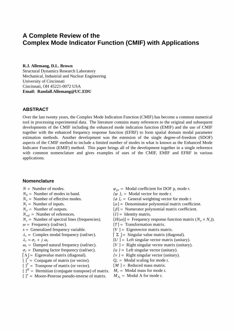
Figure 17. Synthesis Overlay - Real Weighting Vector

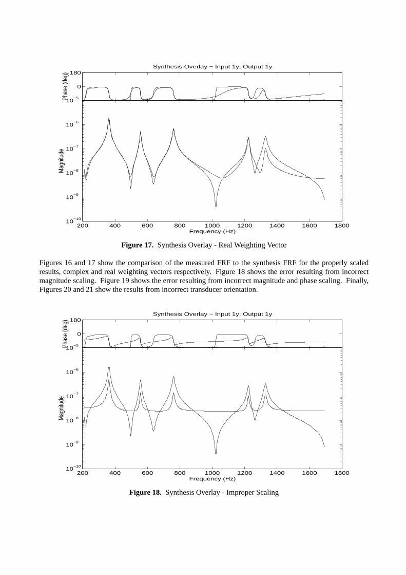
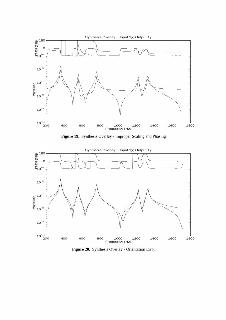
Figures 16 and 17 show the comparison of the measured FRF to the synthesis FRF for the properly scaledresults, complex and real weighting vectors respectively. Figure 18 shows the error resulting from incorrectmagnitude scaling. Figure 19 shows the error resulting from incorrect magnitude and phase scaling. Finally,Figures 20 and 21 show the results from incorrect transducer orientation.

200 400 600 800 1000 1200 1400 1600 180010

−10

10−9

10−8

10−7

10−6

10−5

Frequency (Hz)

Mag

nitu

de

0

180

Phas

e (d

eg)


Figure 18. Synthesis Overlay - Improper Scaling

200 400 600 800 1000 1200 1400 1600 180010

−10

10−9

10−8

10−7

10−6

10−5

Frequency (Hz)

Mag

nitu

de

0

180

Phas

e (d

eg)


Figure 19. Synthesis Overlay - Improper Scaling and Phasing

200 400 600 800 1000 1200 1400 1600 180010

−10

10−9

10−8

10−7

10−6

10−5

Frequency (Hz)

Mag

nitu

de

0

180

Phas

e (d

eg)


Figure 20. Synthesis Overlay - Orientation Error

200 400 600 800 1000 1200 1400 1600 1800−2

−1

0

1

2x 10

−6

Frequency (Hz)

Imag

inary

200 400 600 800 1000 1200 1400 1600 1800−1.5

−1

−0.5

0

0.5

1

1.5x 10

−6

Frequency (Hz)

Real

Figure 21. Synthesis Overlay - Orientation Error

3.1.5 Modal Scaling Methods When the eFRF is formulated so that modal parameters (modalfrequency, modal damping and modal scaling) can be estimated, great care must be taken to get the modalscaling associated with the scaled modal vector. While there are no problems with estimating the modalfrequency and modal damping directly from the eFRF, the normalization of the vector used to formulate theeFRF complicates the estimation of modal scaling since many FRFs are added in a weighted summation todevelop the eFRF.

In order for the eFRF to also be used to estimate the modal scaling (modal mass and/or Modal A), the correctscaling (correct magnitude and phase) of the eFRF must be accounted for. Since the right and left singularvectors in the singular value decomposition are unitary and scaled consistently as a set (but not individually)together with the real valued singular value, the arbitrary scaling of the left singular vector must be accountedfor in the eFRF computation. For this case, where the weighting vector used in the eFRF is estimated fromthe left singular vector associated with a peak in the CMIF plot, the eFRF in general is scaled by utilizing thevalues of the left and right singular vectors, associated with the significant singular value, at the driving pointlocations.

Hunmeasured

H

Figure 22. Frequency Response Space

Note that it is possible that {v} may not be a strict subset of {u}. In this case, the scaling factor must beestimated from the common subset of the input/output degrees of freedom, (ie. the driving point degrees of

freedom).

Several methods have been developed to estimate the proper modal scaling values (modal mass and/or ModalA) in this situation. The following developments summarize the most commonly used methods but the fulldetails of the methods may be found in the references [14-15] . Note that these methods assume that the FRFmatrix is in units of displacement over force.

3.1.5.1 Single Vector Scaling Method The single vector scaling method is the simplest modal scalingmethod in that one mode is enhanced at a time. Since no other modes are involved in the process, significantdistortion may occur at other modal frequencies that will need to be ignored when the modal parameterestimates are estimated using a single degree-of-freedom (SDOF) methods. When the distortion of nearbymodes is significant, a higher order modal parameter estimation method will be required. An example of thisis shown in the next section as the Enhanced Mode Indicator Function (EMIF) Method.

For the following case, a scaled, left singular vector associated with a singular value at one of the peaks ofthe CMIF curves is normally used as the weighting vector ({φ r } = γ {ur}). Any required scaling of thisvector to achieve a specific modal scaling criteria must be performed before the eFRF is estimated. Assumethat in a frequency range of interest, only one mode dominates the FRF matrix:

[H(ω )]No×Ni≈ {ψ }No×1

Qr

( jω − λ r ){ψ }T

1×Ni(24)

Note in the above model, {ψ } is a subset of {ψ } where it is assumed that the number of inputs Ni is lessthan the number of outputs No, the lesser of these two numbers referred to as the number of references Nref .Also, assume that the set of driving point FRF data is complete (Nref = Ni).

Noting that regardless of the normalization of the weighting vector {φ r } used in the eFRF computation, thefollowing squared vector lengths can be defined:

{φ }H {ψ } = C1 = {ψ }H {ψ } (25)

{ψ }T⎧⎨⎩{φ }T ⎫

⎬⎭

H

= {ψ }T {φ }* = C2 = {ψ }T {ψ }* (26)

Now, premultiplying by {φ }T and assuming that the contribution is dominated by the vector product of themode that is being enhanced:

{φ }T [H(ω )] ≈ C1Qr

( jω − λ r ){ψ }T (27)

and postmultiplying by {φ } with the same assumption:

{φ }T [H(ω )] {φ } ≈ C1Qr

( jω − λ r )C2 (28)

eFRFr (ω ) =Qr

( jω − λ r )≈

{φ }T [H(ω )] {φ }

C1 C2(29)

As before, the above equation indicates that the numerator (residue) of the partial fraction that is estimatedfrom the eFRF will be the modal scaling constant Qr modified by the scaling of the two vectors, C1 and C2.In general, though, the two constants are unrelated due to the different lengths of the number of ouputs andnumber of inputs.

Note that, since only one of the modal vectors is used in this formulation, the modal characteristics for themode of interest will be enhanced but so will other modes with a similar spatial pattern. As long as the othermodes are not close in modal frequency, a SDOF modal parameter estimation method will give satisfactoryresults and the residue of the partial fraction, together with the two scaling constants C1 and C2 can be usedto obtain the scaling term Qr and therefore the Modal A or modal mass for the mode of interest.

3.1.5.2 Multi-Vector Scaling Method When more modal vectors have been estimated, the set of modalvectors can be used to estimate the eFRF plots collectively. Some care must be used in the choice of theweighting vecters to be certain that the vectors are not spatially related. This will be discussed further at theend of this section. Beginning with the matrix form of the partial fraction model for the FRF matrix, limitedto a frequency range with Nb modes:

[H(ω )]No×Ni= ⎡

⎣ψ ⎤

⎦No×Nb

⎡⎢⎢

Qr

( jω − λ r )

⎥⎥⎦Nb×Nb

⎡⎣ψ ⎤

⎦

T

Nb×Ni

(30)

Note in the above model, ⎡⎣ψ ⎤

⎦is a subset of ⎡

⎣ψ ⎤

⎦where it is assumed that the number of inputs Ni is less

than the number of outputs No, the lesser of these two numbers referred to as the number of references Nref

as before. The number of modal vectors included in this model is Nb which is the number of modesidentified with the CMIF plot in the frequency band of interest. This may or may not include all modes orthe complex conjugate pairs (negative and positive frequencies) of modes.

In this approach to modal scaling, the scaled, left singular vectors are used as weighting vectors{φ r } = γ {ur}. Note also that any scaling of the left singular vectors to achieve a specific modal scalingcriteria (unity modal coefficient at the driving point, for example) must be performed on the singular vectorsprior to the estimation of the eFRF.

From the definition of pseudo-inverse:

⎡⎣φ ⎤

⎦

+⎡⎣φ ⎤

⎦= [I ] = ⎡

⎣φ ⎤

⎦

+⎡⎣ψ ⎤

⎦(31)

⎡⎣φ ⎤

⎦

T ⎡⎢⎣⎡⎣φ ⎤

⎦

T ⎤⎥⎦

+

= [I ] = ⎡⎣ψ ⎤

⎦

T ⎡⎢⎣⎡⎣φ ⎤

⎦

T ⎤⎥⎦

+

(32)

Note that in the above equations, the matrix⎡⎢⎣⎡⎣φ ⎤

⎦

T ⎤⎥⎦

+

is of dimension Nref × Nb. This means that in order for

the pseudo-inverse to exist, the number of modes that are included must be less than the number of referencesthat are available. Also, based upon the number of references available, two or more of the modal vectorsmay look very similar in spatial distribution. If this occurs, the pseudo-inverse will not exist or be illconditioned and

Therefore, pre-multiplying by ⎡⎣φ ⎤

⎦

+:

⎡⎣φ ⎤

⎦

+[H(ω )] = [I ]

⎡⎢⎢

Qr

( jω − λ r )

⎥⎥⎦

⎡⎣ψ ⎤

⎦

T

(33)

and post-multiplying by⎡⎢⎣⎡⎣φ ⎤

⎦

T ⎤⎥⎦

+

:

⎡⎣φ ⎤

⎦

+[H(ω )]

⎡⎢⎣⎡⎣φ ⎤

⎦

T ⎤⎥⎦

+

≈⎡⎢⎢

Qr

( jω − λ r )

⎥⎥⎦

(34)

At this point, the original weighting vectors (before the pseudo inverse is taken) and modal vectors areassumed to be the identical in order for the identities in Eq. 31 and Eq. 32 to be valid. This means that the

scaling of the modal vectors ⎡⎣φ ⎤

⎦are involved in the computation and, therefore, the modal scaling is with

respect to the normalization used for each vector in ⎡⎣φ ⎤

⎦. Note that, due to the use of the pseudo inverse

vectors as the weighting vectors, the scaling correction is already included (constants C1 and C2 used inprevious methods are automatically 1.0).

Equation 34 represents the Nb eFRFs solved simultaneously via the pseudo inverse. Note that, since a subsetof all theoretical modes is used in this formulation, the resulting matrix may not be purely diagonal asexpected. The diagonal terms of the matrix are the eFRFs for each successive mode and the numerator termin each case is the scaling term Qr which can be directly used to estimate the Modal A or modal mass foreach mode. The diagonal terms will be dominated by the particular mode that is enhanced but may containdistortion or enhancement of other modes as well, depending upon the group of modal vectors included in⎡⎣φ ⎤

⎦. The off-diagonal terms may be ignored (generally) or observed as an indication of the validity of the

formulation.

3.1.5.3 General Singular Vector Scaling Method Since the right and left singular vectors in thesingular value decomposition are unitary and scaled consistently as a set with respect to the real valuedsingular value, these pairs of vectors may be used in a generalized approach to determining the modalscaling. However, the arbitrary scaling of the left and right singular vectors must be accounted for in theeFRF computation. For this general case, where the modal vector used in the eFRF is estimated from the leftsingular vector associated with a peak in the CMIF plot, the eFRF is scaled by utilizing both the left and rightsingular vectors, associated with this significant singular value. In this method, as in most methods of modalscaling, the information in the singular vectors at the driving point locations is very important. While thismethod is completely general, this method is slightly more complicated than the previously presentedmethods.

First of all, assuming operation on only one mode at a time (dropping the mode r notation), also assume thatthe left singular vector is scaled so that it satisfies a required modal scaling method. This generally willmean that the scaled left singular vector is dominantly real. Note that even if the system is proportionallydamped, there is no guarantee that the initial left or right singular vectors will be real valued.

{φ} = {usc} = C3 {u} (35)

This scaled vector {φ} will be the weighting vector that premultiplies the FRF matrix in the computation ofthe eFRF. Now assume that the right singular vector can be projected onto the scaled left singular vector atthe driving point locations (DOFs). The bar notation indicates the subset of the vectors at the Nref common,driving point locations.

{usc} = C4 {v} (36)

The scaling factor, C3, scales and rotates the right singular vector to match the left singular vector at thecommon driving point locations. If the FRF matrix was a theoretical simulation, the scaled right, singularvector should exactly match the scaled, left singular vector. The scaling factor, C4, between the right and leftsingular vectors at the driving point locations can now be defined as follows:

C4 = {v}1×Nref

+ {usc}Nref ×1 (37)

In the above equation, Nref refers to the number of driving point DOFs (DOFs common to both No and Ni

and C4 is a complex scalar. This now allows the complete, scaled right singular vector to be defined:

{vsc} = C4 {v} (38)

The number of elements in the complete, scaled right singular vector {vsc} is Ni where Ni may be equal to,or greater than Nref . Note again that in this formulation the number of inputs Ni is assumed to be smallerthan No and that Nref is the number of common driving point DOFs which is less than or equal to Ni .

The Hermitian of each scaled vector is now used to find the squared length of each vector that will be used inthe estimation of the eFRF.

{usc}H {usc} = C1 {vsc}H {vsc} = C2 (39)

Now the scaled left and right singular vectors can be used to estimate the eFRF as follows:

{usc}T [H(ω )] {vsc} ≈C1 Qr C2

( jω − λ r )(40)

eFRF(ω ) =Qr

( jω − λ r )≈

{usc}T [H(ω )] {vsc}

C1 C2(41)

3.2 Enhanced Mode Indicator Function (EMIF) Method

The Enhanced Mode Indication Function (EMIF) Method is an extension of the CMIF/eFRF method toestimate modal parameters for several modes of vibration at one time. The distinction of this method is thatthe number of poles that are found is fixed based upon the number of peaks identified by the CMIF plots.The flow of this algorithm is as follows:

• Identify the peaks in the CMIF plots.

• Utilize all curves if pseudo-repeated or repeated modal frequencies.

• Use the singular vectors at these peaks to condense the FRF matrix in the long dimension.

• Several frequencies around each peak may be used to estimate one singular vector.

• Form the virtual FRF matrix of dimension number of modes in frequency band of interest bynumber of spectral lines in the frequency range of interest Nb × Ns.

• Estimate the modal frequency and modal damping from a first or second order UMPA model

• First order model if only positive frequency information is used.

• Second order model if positive and negative freqeuncy information is used.

• Fix the size and number of the [α ] coefficients.

• Fix the size but allow the number of [β ] coefficients to be changed.

• Estimate modal scaling using the same methods as CMIF/eFRF

A unique aspect of the EMIF algorithm is that, while the number of poles is fixed based upon the number ossignificant singular values found from the CMIF curves, the number of residuals is allowed to change inorder to develop a consistency diagram approach to finding stable estimates of the modal frequencies.

3.2.1 EMIF Method Details The CMIF plot is first utilized to identify the number of modes Nb in alimited frequency band of interest. The singular vectors for these modes are collected into a tranformationmatrix [T ]:

[T ] = ⎡⎣U⎤

⎦No×Nb

(42)

While this is the simplest explanation for the estimate of the transformation matrix, a number of other

methods have been previously documented [18] that involve utilizing FRF information from severalfrequencies around each peak to estimate the sassociated singular vector. This transformation matrix is usedto create a virtual FRF matrix as follows (assume Nref = Ni):

⎡⎣H(ω )⎤

⎦Nb×Nref

= [T ]TNb×No

[H(ω )]No×Nref(43)

This virtual FRF matrix is then used in a simplified, second order UMPA model as follows:

⎡⎣[α2] ( jω )2 + [α1] ( jω )1 + [α0] ( jω )0⎤

⎦⎡⎣H(ω )⎤

⎦=

nu

k=nl

Σ ⎡⎣[β k] ( jω )k⎤

⎦(44)

or as a first order UMPA model:

⎡⎣[α1] ( jω )1 + [α0] ( jω )0⎤

⎦⎡⎣H(ω )⎤

⎦=

nu

k=nl

Σ ⎡⎣[β k] ( jω )k⎤

⎦(45)

The least squares solution of the above equation is formed based upon the number of frequencies in thefrequency band of interest. Naturally, sufficient frequencies must be included to estimate the number ofunknowns ([α ] and [β ] coefficents). Details on the solution method and the impact of numerical form of themodel is given in other references [12,13,18] .

Note that the size of the [α ] coefficients is Nb × Nb and the size of the [β ] coefficients is Nb × Nref . Thismeans that the second order, matrix coefficient polynomial will always estimate 2Nb roots consistent with thenumber of expected modal frequencies plus the associated complex conjugate roots. If only the positivefrequency information is included in the estimation procedure, the second order term can be eliminatedresulting in the first order UMPA model and Nb roots.

The unique aspect of this algorithm is that the number of [β ] coefficients that are included is varied in orderto generate a consistency diagram. With varying number of [β ] coefficients, this essentially provides avarying number of residual terms to satisfy poorly excited modes or noise and yet always estimate theexpected number of modal frequencies. The same sort of consistency (stability) process used by other modalparameter estimation algorithms is used to choose the best set of modal frequencies to span the modal spacein the frequency range of interest.

4. Representative ApplicationsSeveral applications are included in the text to demonstrate the use and application of CMIF, eFRF and EMIFmethods in developing structural models based upon measured FRF data. The examples in the text to thispoint have been taken from a circular plate that is a relatively easy stucture to test but has nearly identicalrepeated roots associated with many of the peaks in the curves of the CMIF plot. These examples came froma measured FRF matrix for the circular plate that involved 7 output DOFs (No = 7) and 36 input DOFs(Ni = 36). The data was taken using a multiple reference impact testing (MRIT) method using veryconventional testing techniques. The plate is made of steel and is approximately 3 feet (approximately 0.9meter) in diameter with a slightly built-up hub area in the middle of the plate. The thickness of the plate isapproximately 0.75 inches (approximately 2.0 cm) and the hub area is triple the thickness of the plate.

As other representative applications, an analytical example using a 15 DOF model was chosen to illustratethe theoretical aspects of the methods and a very difficult, civil engineering structure was chosen to illustratethe usefulness of the method when the measured FRF data is not ideal. Further details on variousapplications can be found in the references [3,5,6,14,16-19] .

4.1 Analytical 15 DOF Case Study

A 15 DOF analytical system is used to test basic ideas for different levels and kinds of damping as well asclose mode issues. Using this analytical system allows for the modal scaling to be evaluated with respect tothe theoretical answers as well. The portion of the Matlab script used as the basis for the model shown inFigure 22 is documented in the Appendix.

Figure 23. 15 DOF Model

Figures 24 and 25 show the typical CMIF plots for the cases involving the complete FRF matrix and for theimaginary part of the FRF matrix. Some advantage in discriminating close modal frequencies is noticablewhen the imaginary part of the FRF matrix is used.

50 100 150 200 250 30010

−5

10−4

10−3

10−2

10−1

Frequency −− Hz

Com

plex C

MIF

15 DOF Complex CMIF

Figure 24. CMIF from FRF Matrix

50 100 150 200 250 30010

−8

10−7

10−6

10−5

10−4

10−3

10−2

10−1

Frequency −− Hz

Quad

CM

IF

15 DOF Quad CMIF

Figure 25. CMIF from Imaginary Part of FRF Matrix

Figure 26 shows the eFRFs estimated from the complete set of eigenvectors from the analytical solution. If apartial set of eigenvectors are used, some distortion around the modal frequencies would be noticed. Notethat each eFRF curve looks like a SDOF even though no mass matrix was involved in the weightingprocedure. This is due to the pseudo inverse method used in this solution. The pseudo inverse methodmeans that the weighting vectors were the modal filters as developed from the reciprocal modal vectors [11] .

0 50 100 150 200 250 30010

−5

10−4

10−3

10−2

10−1

100

Frequency−−Hz

X/F

EFRF modes 1−15

Figure 26. All eFRFs - Multiple Vector Solution Method for eFRF

Notice that the magnitude scaling on Figure 26 is nearly the same as the magnitude scaling on the CMIF plot.Figures 27 through 30 show the comparison of single vector scaling versus multiple vector scaling. In allcases, the single vector scaling enhances the mode of interest to the point that a SDOF parameter estimationalgorithm can be successfully used to estimate modal parameters as long as the SDOF algortihm has someresduals included. Note that mode 5 and mode 6 have very close modal frequencies.

0 50 100 150 200 250 30010

−5

10−4

10−3

10−2

10−1

Frequency−−Hz

X/F

Comparison EFRF−EFRFs Mode 2

Single Mode −− EFRFsMultiple Mode −− EFRF

Figure 27. Comparison: Single and Multi-Vector Solution for Mode 2

0 50 100 150 200 250 30010

−5

10−4

10−3

10−2

Frequency−−Hz

X/F




0 50 100 150 200 250 30010

−5

10−4

10−3

10−2

10−1

Frequency−−Hz

X/F




0 50 100 150 200 250 30010

−4

10−3

10−2

10−1

Frequency−−Hz

X/F



Figure 30. Comparison Single and Multi-Vector Solution for Mode 12

4.2 Bridge Case Study

The final test case involves a 15 reference impact test on a civil engineering bridge structure. The FRF datafrom this structure is notoriously difficult to fit using any traditional algorithm and to date the best resultshave been obtained by using spatial domain modal parameter estimation methods such as CMIF/eFRF andEMIF [14,16] . This includes recent attempts to fit the original data with all methods included in the UMPAframework [19] that includes methods like PTD, ERA, PFD and the latest Polyreference Least SquaresComplex Frequency (PLSCF) method.

Figure 31. Seymour Street Bridge, Cincinnati, Ohio, USA

The civil engineering bridge structure that was tested is the Seymour Street Bridge in Cincinnati, Ohio shownin Figure 31.

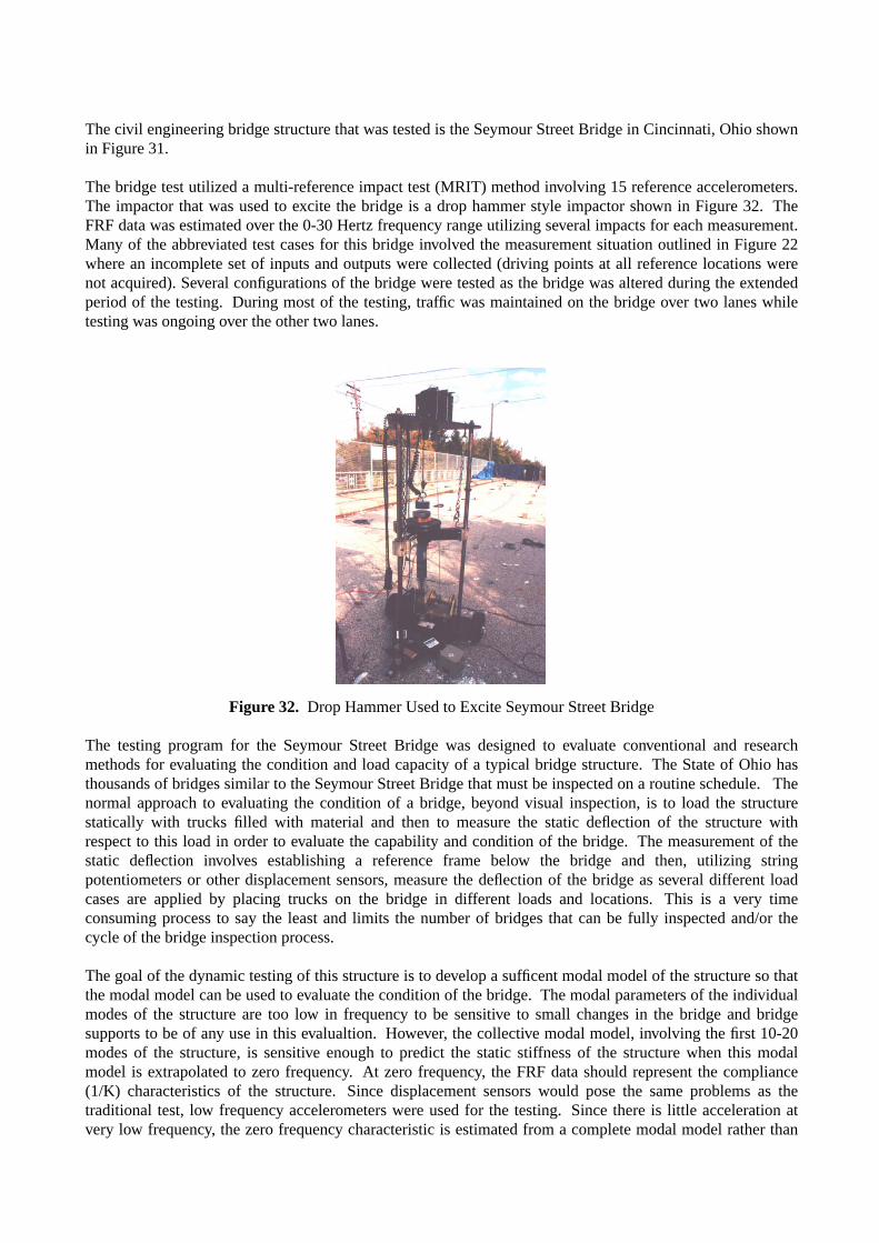
The bridge test utilized a multi-reference impact test (MRIT) method involving 15 reference accelerometers.The impactor that was used to excite the bridge is a drop hammer style impactor shown in Figure 32. TheFRF data was estimated over the 0-30 Hertz frequency range utilizing several impacts for each measurement.Many of the abbreviated test cases for this bridge involved the measurement situation outlined in Figure 22where an incomplete set of inputs and outputs were collected (driving points at all reference locations werenot acquired). Several configurations of the bridge were tested as the bridge was altered during the extendedperiod of the testing. During most of the testing, traffic was maintained on the bridge over two lanes whiletesting was ongoing over the other two lanes.

Figure 32. Drop Hammer Used to Excite Seymour Street Bridge

The testing program for the Seymour Street Bridge was designed to evaluate conventional and researchmethods for evaluating the condition and load capacity of a typical bridge structure. The State of Ohio hasthousands of bridges similar to the Seymour Street Bridge that must be inspected on a routine schedule. Thenormal approach to evaluating the condition of a bridge, beyond visual inspection, is to load the structurestatically with trucks filled with material and then to measure the static deflection of the structure withrespect to this load in order to evaluate the capability and condition of the bridge. The measurement of thestatic deflection involves establishing a reference frame below the bridge and then, utilizing stringpotentiometers or other displacement sensors, measure the deflection of the bridge as several different loadcases are applied by placing trucks on the bridge in different loads and locations. This is a very timeconsuming process to say the least and limits the number of bridges that can be fully inspected and/or thecycle of the bridge inspection process.

The goal of the dynamic testing of this structure is to develop a sufficent modal model of the structure so thatthe modal model can be used to evaluate the condition of the bridge. The modal parameters of the individualmodes of the structure are too low in frequency to be sensitive to small changes in the bridge and bridgesupports to be of any use in this evalualtion. However, the collective modal model, involving the first 10-20modes of the structure, is sensitive enough to predict the static stiffness of the structure when this modalmodel is extrapolated to zero frequency. At zero frequency, the FRF data should represent the compliance(1/K) characteristics of the structure. Since displacement sensors would pose the same problems as thetraditional test, low frequency accelerometers were used for the testing. Since there is little acceleration atvery low frequency, the zero frequency characteristic is estimated from a complete modal model rather than

from direct measurement. Using this test method, a single test could be completed in several hours ratherthan several days.

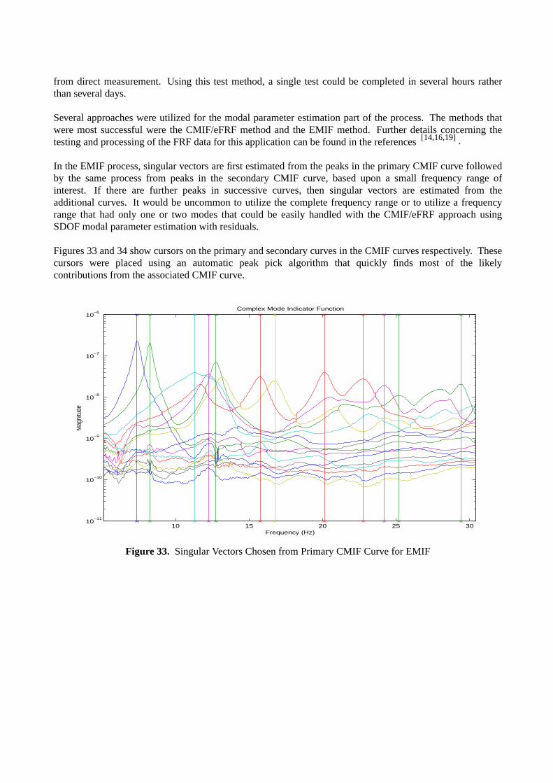
Several approaches were utilized for the modal parameter estimation part of the process. The methods thatwere most successful were the CMIF/eFRF method and the EMIF method. Further details concerning thetesting and processing of the FRF data for this application can be found in the references [14,16,19] .

In the EMIF process, singular vectors are first estimated from the peaks in the primary CMIF curve followedby the same process from peaks in the secondary CMIF curve, based upon a small frequency range ofinterest. If there are further peaks in successive curves, then singular vectors are estimated from theadditional curves. It would be uncommon to utilize the complete frequency range or to utilize a frequencyrange that had only one or two modes that could be easily handled with the CMIF/eFRF approach usingSDOF modal parameter estimation with residuals.

Figures 33 and 34 show cursors on the primary and secondary curves in the CMIF curves respectively. Thesecursors were placed using an automatic peak pick algorithm that quickly finds most of the likelycontributions from the associated CMIF curve.

10 15 20 25 3010

−11

10−10

10−9

10−8

10−7

10−6


Frequency (Hz)

Mag

nitu

de

Figure 33. Singular Vectors Chosen from Primary CMIF Curve for EMIF

10 15 20 25 3010

−11

10−10

10−9

10−8

10−7

10−6


Frequency (Hz)

Mag

nitu

de

Figure 34. Singular Vectors Chosen from Secondary CMIF Curve for EMIF

In this example, twelve peaks were initially found from the primary curve and two peaks were found fromthe secondary curve. Additional peaks can then be added manually to account for any peaks that weremissed by the automatic process. In this example, one more peak was added manually. The CMIF/eFRFapproach gav e satisfactory results for most modes except for the five modes in the 11-14 Hertz frequencyrange. Figures 35 through 39 show the eFRF results for several of these modes. Note the dotted linesrepresenting the synthesis of the associated SDOF model. Note also the phasing error at zero frequency dueto the sensor orientation inconsistency.

10 15 20 25 30−180

0

180CMIF − Enhanced Frequency Response Function

Frequency (Hz)

Phas

e

10 15 20 25 3010

−10

10−9

10−8

10−7

10−6

CMIF − Enhanced Frequency Response Function

Frequency (Hz)

Mag

nitu

de

Figure 35. eFRF for 7.35 Hertz Mode

10 15 20 25 30−180

0


Frequency (Hz)

Phas

e

10 15 20 25 3010

−10

10−9

10−8

10−7

10−6


Frequency (Hz)

Mag

nitu

de


10 15 20 25 30−180

0


Frequency (Hz)

Phas

e

10 15 20 25 3010

−10

10−9

10−8

10−7

10−6


Frequency (Hz)

Mag

nitu

de


10 15 20 25 30−180

0


Frequency (Hz)

Phas

e

10 15 20 25 3010

−10

10−9

10−8

10−7

10−6


Frequency (Hz)

Mag

nitu

de


10 15 20 25 30−180

0


Frequency (Hz)

Phas

e

10 15 20 25 3010

−10

10−9

10−8

10−7


Frequency (Hz)

Mag

nitu

de


The five peaks found in the 11-14 Hertz frequency range were then used to identify the five singular vectorsto be used in the EMIF method. The five singular vectors were used to transform the FRF data matrix to thefive virtual (modal) DOFs associated with these vectors. Note that at this point, the virtual FRF matrix is ofdimension 5 × 15 where the number of references is 15 (Nref = 15). The five peaks are identified in Figure40, at the top of the EMIF plots, with solid triangles (note that two peaks are very close together infrequency).

9 10 11 12 13 14 1510

−11

10−10

10−9

10−8

10−7

Enhanced Mode Indicator Function

Frequency (Hz)

Mag

nitu

de

Figure 40. EMIF Results for Five Modes between 11 and 14 Hertz

Using this transformed FRF data matrix in a second order model as described in Section 3.2, the modalparameters were estimated for the five modes of interest while allowing the number of residuals to vary in theconsistency diagram. Note the dotted lines in Figure 40 that are used to show the synthesis compared to thevirtual eFRFs. Note also that there are only five dominant contributions in this frequency range (nonoticeable modes in the remaining 10 eFRFs shown).

Figure 41. Modal Model Correlation with Static Deflection Test

Figure 41 summarizes the results of one of the load cases studied using this approach to determining the

static deflection characterisitics of the Seymour Street bridge. The green curve on the figure represents thestatic deflection predicted from the modal model developed using CMIF/eFRF and EMIF methods. Thepurple curve in the figure represents the actual deflection measured by the normal static deflection test whilethe trucks were in position on the bridge. Note that this is a representative result from several load cases thatwere compared. In this case, the first fifteen modes in the modal model were used to predict the staticdeflection curve from the compliance (1/K) of the associated, synthesized FRF data.

5. Summary and Conclusions

Over the last twenty years, the Complex Mode Indicator Function (CMIF) has become a powerful method fordetecting and analyzing repeated root or pseudo-repeated root situations in FRF data. Combining the modalvector estimates from the singular vectors of peaks in the CMIF curves with the modal frequency and modalscaling estimates produced by the Enhanced Frequency Response Function (eFRF) results in an effective,efficient modal parameter estimation technique that can be used even when the FRF data is non-ideal. TheEMIF method extends the SDOF nature of the CMIF/eFRF to the point that very difficult frequency rangescan be handled. These methods have been used successfully on many different types of structures and on datathat was not amenable to more sophisticated techniques. However, as has been shown, strict attention mustbe paid to the magnitude and phase scaling of the eFRF in order to extract reliable estimates for modalscaling (Modal A or modal mass). Failure to properly scale the eFRF yields estimates that, while resonablyaccurate with respect to modal frequency, modal damping and modal vector, are improperly scaled andtherefore unsuitable for more rigorous applications such as impedance and modal modeling or operatingloads prediction.

6. References[1] Shih, C.Y., Tsuei, Y.G., Allemang, R.J., and Brown, D.L., "Complex Mode Indicator Function and Its

Applications to Spatial Domain Parameter Estimation" Proceedings, 13th International Seminar onModal Analysis, Katholieke Universiteit Leuven, Belgium, 15 pp., 1988.

[2] Shih, C.Y., Tsuei, Y.G., Allemang, R.J., Brown, D.L., "Complex Mode Indication Function and ItsApplication to Spatial Domain Parameter Estimation", Mechanical System and Signal Processing,Vol. 2, No. 4, pp. 367-377, 1988.

[3] Coleman, A.D., Driskill, T.C., Anderson, J.B., Brown, D.L., "A Mass Additive Technique for ModalTesting as Applied to the Space Shuttle Astro-1 Payload", Proceedings, International Modal AnalysisConference, 7 pp., 1988.

[4] Shih, C.Y., Tsuei, Y.G., Allemang, R.J., and Brown, D.L., "Complex Mode Indicator Function and ItsApplications to Spatial Domain Parameter Estimation" Proceedings, International Modal AnalysisConference, pp. 533540, 1989.

[5] Shih, C.Y., "Investigation of Numerical Conditioning in the Frequency Domain Modal ParameterEstimation Methods", Doctoral Dissertation, University of Cincinnati, 1989, 127 pp.

[6] Allemang, R.J., Brown, D.L., Fladung, W., "Modal Parameter Estimation: A Unified MatrixPolynomial Approach", Proceedings, International Modal Analysis Conference, pp. 501-514, 1994.

[7] Phillips, A.W., Allemang, R.J., "The Unified Matrix Polynomial Approach to Understanding ModalParameter Estimation: An Update", Proceedings, International Conference on Noise and VibrationEngineering, Katholieke Universiteit Leuven, Belgium, 36 pp., 2004.

[8] Leurs, W., Deblauwe, F., Lembregts, F., "Modal Parameter Estimation Based Upon Complex ModeIndicator Functions", Proceedings, International Modal Analysis Conference, pp. 1035-1041, 1993.

[9] Phillips, A.W., Allemang, R.J., "The Complex Mode Indicator Function (CMIF) as a ParameterEstimation Method", Proceedings, International Modal Analysis Conference, pp. 705-710, 1998.

[10] Allemang, R. J., "Investigation of Some Multiple Input/Output Frequency Response FunctionExperimental Modal Analysis Techniques", Doctoral Dissertation, University of Cincinnati, 1980,358 pp.

[11] Shelley, S.J., "Investigation of Discrete Modal Filters for Structural Dynamic Applications", DoctoralDissertation, University of Cincinnati, 269 pp., 1991.

[12] Fladung, W.A., Phillips, A.W., Brown, D.L., "Specialized Parameter Estimation Algorithms forMultiple Reference Testing", Proceedings, International Modal Analysis Conference, pp. 1078-1087,1997.

[13] Fladung, W.A., Phillips, A.W., Brown, D.L., "The Development of an Enhanced Mode IndicatorFunction Parameter Estimation Algorithm", ASME Design Engineering Technical Conference, 1997.

[14] Catbas, F.N., "Investigation of Global Condition Assessment and Structural Damage Identification ofBridges with Dynamic Testing and Modal Analysis", Doctoral Dissertation, University of Cincinnati,198 pp., 1997.

[15] Phillips, A.W., Allemang, R.J., "The Enhanced Frequency Response Function (eFRF): Scaling andOther Issues", Proceedings, International Conference on Noise and Vibration Engineering, Volume 1,Katholieke Universiteit Leuven, Belgium, 8 pp., 1998.

[16] Catbas, F.N., Lenett, M., Aktan, A.E., Brown, D.L., Helmicki, A.J., and Hunt, V.J., "DamageDetection and Condition Assessment of Seymour Bridge" Proceedings, International Modal AnalysisConference, pp. 1694-1702, 1998.

[17] Li, S., Fladung, W.A., Phillips, A.W., Brown, D.L., "Automotive Applications of the Enhanced ModeIndicator Function Parameter Estimation Method", Proceedings, International Modal AnalysisConference, pp. 36-44, 1998.

[18] Fladung, W.A., "A Generalized Residuals Model for The Unified Matrix Polynomial Approach toFrequency Domain Modal Parameter Estimation", Doctoral Dissertation, University of Cincinnati,152 pp., 2001.

[19] Catbas, F.N., Brown, D.L., Aktan, A.E., "Parameter Estimation for Multiple-Input Multiple-OutputModal Analysis of Large Structures", Journal of Engineering Mechanics, Volume 130, Issue 8, pp.921-930, 2004.

[20] Strang, G., Linear Algebra and Its Applications, Third Edition, Harcourt Brace JovanovichPublishers, San Diego, 1988, 505 pp.

[21] Lawson, C.L., Hanson, R.J., Solving Least Squares Problems, Prentice-Hall, Inc., EnglewoodCliffs, New Jersey, 1974, 340 pp.

Appendix A: 15 DOF Matlab Model

%% Generating M C K matrices for 15 DOF Model%

NN=5; % DOF’s equals 3*NN

m1=10/386.09;m2=10/386.09;m3=.5/386.09;k1=1000;k2=1000;k3=1000;k4=1000;c1=.2;c2=.2;c3=.05;c4=.2;

rand1=[0 -100 100 -200 200];

for kk=1:NN,M1(kk,kk)=m1;M2(kk,kk)=m2;M3(kk,kk)=m3;K1(kk,kk)=2*k1+k3+k4+rand1(kk);K2(kk,kk)=2*k2+k4;K3(kk,kk)=k3+rand1(kk);K12(kk,kk)=-k4;K13(kk,kk)=-k3-rand1(kk);C1(kk,kk)=2*c1+c3+c4;C2(kk,kk)=2*c2+c4;C3(kk,kk)=c3;C12(kk,kk)=-c4;C13(kk,kk)=-c3;

end

for kk=1:NN-1,K1(kk,kk+1)=-k1;K1(kk+1,kk)=-k1;K2(kk,kk+1)=-k2;K2(kk+1,kk)=-k2;C1(kk,kk+1)=-c1;C1(kk+1,kk)=-c1;C2(kk,kk+1)=-c2;C2(kk+1,kk)=-c2;

end

M(1:NN,1:NN)=M1;M(NN+1:2*NN,NN+1:2*NN)=M2;M(2*NN+1:3*NN,2*NN+1:3*NN)=M3;

K(1:NN,1:NN)=K1;K(NN+1:2*NN,NN+1:2*NN)=K2;K(2*NN+1:3*NN,2*NN+1:3*NN)=K3;K(NN+1:2*NN,1:NN)=K12;K(1:NN,NN+1:2*NN)=K12;K(2*NN+1:3*NN,1:NN)=K13;K(1:NN,2*NN+1:3*NN)=K13;C(1:NN,1:NN)=C1;C(NN+1:2*NN,NN+1:2*NN)=C2;C(2*NN+1:3*NN,2*NN+1:3*NN)=C3;C(NN+1:2*NN,1:NN)=C12;C(1:NN,NN+1:2*NN)=C12;C(2*NN+1:3*NN,1:NN)=C13;C(1:NN,2*NN+1:3*NN)=C13;

a complete review of the complex mode indicator …€¦ · a complete review of the complex mode...

Documents