a computational and experimental modelling of thermo-hydro

A COMPUTATIONAL AND EXPERIMENTAL MODELLING OF

THERMO-HYDRO-MECHANICAL PROCESSES IN A LOW

PERMEABILITY GRANITE

by

Meysam Najari

August, 2013

Department of Civil Engineering and Applied Mechanics

McGill University, Montreal

A thesis submitted to

McGill University

in partial fulfillment of the requirements of the degree of

Doctor of Philosophy

© 2013 Meysam Najari

To my parents and my sister

iii

ABSTRACT

This thesis deals with the computational and experimental study of non-

isothermal fluid transport in Stanstead Granite, a low-permeability rock. The

study has several topics of interest to modern environmental geomechanics. These

include the deep geologic disposal of heat-emitting nuclear fuel wastes, the

extraction of geothermal energy, oil and gas recovery, and the geologic

sequestration of carbon dioxide in supercritical form.

The equations governing the fully-coupled isothermal and non-isothermal

behaviour of linear elastic porous geomaterials are presented and a finite element

scheme is used to solve these equations. The basic physical and mechanical

properties of Stanstead Granite are determined through a series of standard

experiments. The permeability characteristics of the selected rock type were

investigated using both steady state and hydraulic pulse testing techniques. The

range of applicability of the conventional piezo-conduction equation for the

interpretation of hydraulic pulse test results was investigated by comparing the

fluid decay curves obtained form the solution of both the linear poroelastic

equations and piezo-conduction equation for two typical rock types: Indiana

Limestone and Westerly Granite. A series of hydraulic pulse tests were performed

on Stanstead Granite samples at the bench-scale with different geometries and

boundary conditions. It was observed that regardless of how precisely the cavity

was filled with de-aired water, air bubbles can still exist in the cavity and this air

fraction can influence the results of hydraulic pulse tests. A novel technique is

suggested for taking into account the influence of the volume of trapped air and

eliminating its effect on the estimation of permeability. The alteration of

permeability of Stanstead Granite under isotropic loading and unloading using

steady state permeability measurement technique was also examined. The

iv

applicability of conventional THM models for the characterization of the

Stanstead Granite subjected to heating was investigated. The experiments used in

the research included THM tests on a cylindrical sample of saturated Stanstead

Granite containing a fluid-filled cylindrical cavity. An apparatus capable of

changing the temperature in a controlled fashion was designed and fabricated. The

outer boundaries of the specimen were subjected to cycles of heating and cooling

and the temperature and fluid pressure in the sealed cavity were recorded. The

results obtained in the simulations compared favourably with measured

temperature and pore pressure values.

v

RÉSUMÉ

Cette dissertation étudie le transport fluide non-isotherme dans le granite de

Stanstead, une roche de faible perméabilité, au moyen de simulations numériques

et de tests expérimentaux. Elle est relative à plusieurs questions d'intérêt en

géomécanique environnementale, dont notamment le stockage en couches

géologiques profondes de déchets nucléaires actifs, l'extraction d'énergie d'origine

géothermique, l'extraction de gaz et de pétrole, et le stockage géologique de

dioxyde de carbone supercritique.

Les équations décrivant le comportement couplé isotherme et non-isotherme des

(géo) matériaux poreux linéaires élastiques sont présentées, et la méthode des

éléments finis est utilisée pour les résoudre. Les principales caractéristiques

physiques et mécaniques du granite de Stanstead sont déterminées via une série de

tests expérimentaux standards. Les propriétés de perméabilité du type de roche

choisie sont investiguées à la fois au moyen de tests stationnaires et de techniques

utilisant des impulsions hydrauliques. Le domaine de validité de l'équation

conventionnelle de piézo-conduction pour l'interprétation de ces tests d'impulsion

hydraulique est investigué en comparant les courbes de décroissance de pression

fluide obtenues par les solutions de la poroélasticité linéaire et l'équation de piézo-

conduction pour deux roches types: le calcaire d'Indiana et le granite de

Westerley.

Une série de tests d'impulsion hydraulique est réalisée sur des échantillons de

granite de Stanstead à l'échelle du laboratoire pour différentes géométries

d'échantillon et différentes conditions aux limites. Indépendamment de la

précision avec laquelle la cavité est remplie d'eau supposée ne pas contenir d'air,

des bulles d'air sont observées dans la cavité, et leur présence influence les

résultats obtenus par les techniques d'impulsion hydraulique. Une nouvelle

technique est alors suggérée pour prendre en compte l'influence du volume d'air

inclus, et éliminer son effet sur l'estimation de la perméabilité. La modification de

vi

la perméabilité du granite de Stanstead sous chargement et déchargement isotrope

est également analysée au moyen de tests de perméabilité stationnaires.

L'applicabilité des modèles thermo-hydro-mécaniques pour la caractérisation du

granite de Stanstead soumis à échauffement a également est aussi investiguée. Les

tests expérimentaux utilisés dans cette partie de la recherche comprennent

notamment des tests thermo-hydro-mécaniques appliqués à un cylindre de granite

de Stanstead saturé contenant une cavité cylindrique remplie de fluide. Un

équipement en vue de modifier la température de façon contrôlée a été conçu et

réalisé, permettant de soumettre les frontières extérieures du spécimen à des

cycles d'échauffement et de refroidissement, tout en enregistrant la température et

la pression de fluide dans la cavité isolée. Les résultats obtenus par simulation

présentent un bon accord avec les mesures de température et de pression.

vii

ACKNOWLEDGEMENS

The author would like to express his immense appreciation to his supervisor,

Professor A.P.S. Selvadurai for suggesting the topic of the research, continuous

and extensive guidance and mentoring, and the sustained encouragement and

support throughout the entire thesis program. The author feels deeply indebted for

all he learned from his supervisor.

The author is grateful to his colleagues in the Geomechanics Group at the

Department of Civil Engineering and Applied Mechanics, McGill University for

their support and assistance; namely, Mr. L. Jenner, Mr. B. Hekimi, Mr. A.

Glowacki, Mr. P. Selvadurai, Dr. A. Suvorov, Mr. A. Katebi, Mr. D. Cuneo, Mr.

M. Boyd, and Mr. A. Gallagher. The author would also like to acknowledge the

extensive technical assistance he received from Mr. J. Bartczak, Dr. W. Cook, Mr.

S. Kecani, Mr. G. Bechard, and Mr. M. Przykorski in design, fabrication and

assembly of the experimental facilities he used over the course of the research.

The author is also thankful of Ms. G. Keating from the Department of Earth and

Planetary Sciences, McGill University for conducting an XRF test and Mr. L.

Martinez from the Department of Building, Civil and Environmental Engineering,

Concordia University for conducting an MIP test. Special thanks are due to Mrs.

Sally Selvadurai for her extensive editorial corrections of the current thesis and all

the papers that resulted from the research. Sincere thanks go to Professor Thierry

Massart, Université Libre de Bruxelles, for his assistance in translating the

abstract of this thesis to French.

The research conducted in this thesis was supported by NSERC Strategic and

Discovery Grants awarded to Professor A.P.S. Selvadurai, as well as the support

of the NWMO. The author also wishes to acknowledge the financial support he

received from Global, Environmental and Climate Change Center, Montreal,

through FQRNT.

viii

Finally, the author would like to express his deepest thanks to his parents and his

sister who provided him with nothing but support and love throughout the course

of this research. This thesis is dedicated to them.

ix

TABLE OF CONTENTS

ABSTRACT iii

RÉSUMÉ v

ACKNOWLEDGMENTS vii

LIST OF TABLES xiii

LIST OF FIGURES xv

LIST OF PUBLICATIONS xxiv

1 INTRODUCTION AND LITERATURE REVIEW

1.1 General 1

1.2 Isothermal poroelasticity 4

1.3 Permeability 7

1.4 Non-isothermal poroelasticity 12

1.5 Objectives and scope of the research 15

2 MECHANICAL AND PHYSICAL CHARACTERIZATION OF

STANSTEAD GRANITE

2.1 General description 17

2.2 Chemical composition 18

2.3 Porosity 19

2.3.1 Conventional saturation test 20

2.3.2 Mercury intrusion porosimetry 21

2.4 Elasticity parameters and compressive strength 26

2.5 Tensile strength 29

2.6 Summary remarks 30

3 MECHANICS OF ISO-THERMAL POROELASTIC MEDIA

3.1 Introduction 33

x

3.2 Terzaghi’s theory of consolidation 34

3.3 Theory of linear poroelasticity 37

3.3.1 Governing equations 38

3.3.2 Skempton’s coefficient 40

3.3.3 Constrained specific storage 40

3.3.4 Fluid phase equation 41

3.3.5 Solid phase equation 43

3.3.6 Uncoupling stress from pore pressure 44


4 PERMEABILITY MEASUREMENT: THEORY AND

EXPERIMENT

4.1 Introduction 47

4.2 Hydraulic pulse testing: theory 48

4.2.1 Governing equations 49

4.2.2 Theoretical modelling 51

4.2.3 Computational study of the effect of poroelastic coupling 54

4.2.4 The effect of aspect ratio on the coupling behaviour 65

4.3 Hydraulic pulse testing: experiment 68

4.3.1 Radially symmetric hydraulic pulse tests 69

4.3.2 Patch pulse tests 74


5 THE EFFECT OF AIR BUBBLES ON THE INTERPRETATION

OF HYDRAULIC PULSE TESTS

5.1 Introduction 80

5.2 Governing equations 81

5.3 Computational modelling of the effect of air inclusion on hydraulic 84

pulse tests

5.4 Permeability measurement of the small size sample 86

xi

5.4.1 Steady state tests 87

5.4.2 Hydraulic pulse tests 88

5.4.3 Back-calculation of compressibility change from the experiment 90

5.4.4 Estimation of permeability range 92

5.4.5 Injecting air in the cavity 94

5.5 Permeability measurement of the large sample 97

5.5.1 Steady state tests 98

5.5.2 Hydraulic pulse tests 99


6. PERMEABILITY HYSTERESIS UNDER ISOTROPIC

COMPRESSION

6.1 Introduction 104

6.2 Sample preparation 105

6.3 Testing facility and sample assembly 107

6.4 Steady state permeability measurement 109

6.4.1 Steady state test results 110

6.4.2 Discussion on the steady state test results 113


7 THERMO-HYDRO-MECHANICS OF POROUS

GEOMATERIALS

7.1 Introduction 116

7.2 Governing equations 117

7.2.1 The constitutive equation for the porous solid 117

7.2.2 Liquid phase equation 117

7.2.3 Energy equation 119

7.2.4 Computational modelling of fluid inclusion 120

7.3 Thermal damage experiment 122

7.3.1 Testing procedure 123

xii

7.4 Immersion thermal experiment 125

7.4.1 Permeability measurement 126

7.4.2 Thermo-hydro-mechanical experiment 128

7.4.3 Experimental results and numerical simulations 129

7.5 Thermo-hydro-mechanical experiment under controlled 133

temperature changes

7.5.1 The testing apparatus 133

7.5.2 Permeability measurement 135

7.5.3 Thermo-hydro-mechanical experiment 138

7.5.4 Experimental results and computational modelling 140

7.6 Summary 148

8 CONCLUSIONS AND SCOPE FOR FUTURE RESEARCH

8.1 Summary and concluding remarks 151

8.2 Scope for future research 155

REFERENCES 158

APPENDIX A: Petrological description of Stanstead Granite 176

(unpublished report)

xiii

LIST OF TABLES

Table 2.1 The weight percentage of the chemical compounds of

Stanstead Granite, compared with similar igneous rocks.

19

Table 2.2 Details of the measurements and calculations done to

Measure the porosity of Stanstead Granite.

20

Table 2.3 Experimental results of MIP tests performed on three

samples of Stanstead Granite.

26

Table 2.4 The result of the splitting tensile strength tests performed on

four samples of Stanstead Granite.

30

Table 2.5 The measured physical parameters compared to similar

values available in the literature.

31

Table 2.6 Comparison of the UCS test results with similar results

available in the literature.

32

Table 4.1 The mechanical, physical and hydraulic parameters

applicable to Westerly Granite and Indiana Limestone.

61

Table 4.2 Storativity terms for Westerly Granite and Indiana

Limestone.

62

Table 4.3 Permeability values for Stanstead Granite 74

Table 5.1 The results of steady state tests performed on Stanstead

Granite sample S-SG.

88

Table 5.2 The results of steady state tests performed on the large

sample of Stanstead Granite, L-SG.

98

Table 6.1 Steady state permeability tests on Stanstead Granite sample

GDS1 at various confining pressures.

111

Table 6.2 Steady state permeability of Stanstead Granite Sample GDS2

at different confining pressures.

112

xiv

Table 6.3 Steady state permeability of Stanstead Granite sample GDS3

at different confining pressures.

112

Table 6.4 Change in the degree of anisotropy ( 2 3GDS GDSK K ) with the

change of isotropic compression.

114

Table 7.1 Range of values of permeability before and after thermal

loading.

125

Table 7.2 The results of sealing tests performed on a stainless steel

cylinder.

138

Table 7.3 Values of the parameters in the computational modelling of

the THM experiment.

144

xv

LIST OF FIGURES

Figure 1.1 Conceptual layout of the deep geological repository site

below the Bruce site, Ontario, Canada (OPG, 2008).

3

Figure 1.2 The apparatus used by Darcy for the study of fluid flow

through soils (Courtesy of Prof. Olivier Coussy, LCPC,

Paris)

5

Figure 1.3 Changes in the pore pressure with time in the center of a

sphere subjected to compressive surface traction

(reproduced after Gibson et al., 1963)

7

Figure 2.1 The MIP testing apparatus at the Building Materials

Laboratories at Concordia University.

22

Figure 2.2 The penetrometer with the bulb filled with mercury at the

end of the low pressure range test.

23

Figure 2.3 Equilibrium of forces acting inside a capillary; forcing

(F1) and opposing (F2) mercury intrusion into the

capillary (after Aligizaki, 2006)

23

Figure 2.4 Cumulative porosity change versus pore diameter for

samples A, B, and C.

25

Figure 2.5 The Stanstead Granite cylinder, instrumented with two

rosette strain gauges prepared for the uniaxial

compressive test.

27

Figure 2.6 Axial stress-axial strain curve for an unconfined

compression test performed on a Stanstead Granite

sample.

27

xvi

Figure 2.7 The axial stress-strain curve for the last unloading curve

before failure of the Stanstead Granite sample

28

Figure 2.8 The change of circumferential strain with axial strain for

the last unloading cycle before failure in a Stanstead

Granite sample.

28

Figure 2.9 The testing assembly used for performing Brazilian

tensile strength tests (the assembly is shown from two

different angles).

30

Figure 4.1 Geometry and boundary conditions assumed for the

axisymmetric one-dimensional stress hydraulic pulse test.

55

Figure 4.2 Geometry and boundary conditions assumed for the one-

dimensional strain hydraulic pulse test.

55

Figure 4.3 Schematic view for the radially symmetric hydraulic

pulse testing of an infinitely extended rock mass

58

Figure 4.4 The geometry and boundary conditions of the problem

examined by Hart and Wang (1998).

58

Figure 4.5 Comparison of the results obtained by Hart and Wang

(1998) with the results of the current study. The figure

also shows the detail of the initial 120 seconds and the

geometry and boundary conditions of the problem.

60

Figure 4.6 Mesh configuration for modelling: (a) one-dimensional

hydraulic pulse test (25028 elements), (b) radially

symmetric hydraulic pulse test (30017 elements).

62

xvii

Figure 4.7 Comparison of the pressure decay curves obtained from

Biot’s theory of poroelasticity with those obtained using

the piezo-conduction equation for the one-dimensional

hydraulic pulse test.

63

Figure 4.8 Comparison of the pressure decay curves obtained from

Biot’s theory of poroelasticity with those obtained using

the piezo-conduction equation for a radially symmetric


64

Figure 4.9 Comparison of the computational results obtained from

the Biot poroelasticity equations with the piezo-

conduction equation for one-dimensional constant stress

and constant strain hydraulic pulse testing for different

aspect ratios.

67

Figure 4.10 Comparison of the computational results obtained from

the Biot poroelasticity equations with the piezo-

conduction equation for radially symmetric hydraulic

pulse testing for different aspect ratios.

68

Figure 4.11 Experimental faculty for measuring the permeability of

low permeability geomaterials (Frame designed by Mr. A.

Chevrier, Carleton University).

70

Figure 4.12 Components of the permeameter used to perform

hydraulic pulse tests on fully-drilled samples.

71

Figure 4.13 Decay of cavity pressure in 3 hydraulic pulse tests

performed on a dummy aluminum cylinder, using an O-

ring for the sealing.

72

xviii

Figure 4.14 Results of hydraulic pulse tests performed on a fully

drilled Stanstead Granite cylinder (sample SD). The

analysis of the data was done using the piezo-conduction

equation and neglecting the compressibility of the solid

grains.

73

Figure 4.15 Decay of cavity pressure in hydraulic pulse tests

performed on a Plexiglas, using gasket for the sealing.

75

Figure 4.16 Components of the permeameter used to perform

hydraulic pulse tests on undrilled samples.

75

Figure 4.17 Results of hydraulic pulse tests performed on an undrilled

Stanstead Granite cylinder (sample SU). The analysis of

data was done using the piezo-conduction equation and

neglecting the compressibility of the solid grains.

76

Figure 4.18 Sample SU: (a) Geometry and boundary conditions used

for the piezo-conduction equation; (b) Geometry and

boundary conditions used for Biot’s poroelasticity

equations.

77

Figure 5.1 Compressibility of air-water mixtures with different air

fractions.

83

Figure 5.2 The geometry and boundary conditions of the one-

dimensional hydraulic pulse test.

85

Figure 5.3 Effect of air bubbles on cavity pressure decay. 85

Figure 5.4 The assembly of sample S-SG. 86

xix

Figure 5.5 Schematic view of the hydraulic pulse test experiment

performed on sample S-SG.

87

Figure 5.6 Changes in cavity pressure for steady state tests

performed on Stanstead Granite sample S-SG, at different

flow rates.

88

Figure 5.7 Hydraulic pulse tests performed on sample Stanstead

Granite S-SG.

89

Figure 5.8 Change of eqC with cavity pressure increase in Stanstead


91

Figure 5.9 Experimental results for the build-up of cavity pressure

due to pumping water at the rate of Q =2ml/min, for

Stanstead Granite sample S-SG.

92

Figure 5.10 Hydraulic pulse test results performed on Stanstead

Granite sample S-SG with a maximum cavity pressure of

120 kPa.

93



265 kPa.

94

Figure 5.12: Hydraulic pulse test results performed on Stanstead


660 kPa.

94


due to pumping water at the rate of Q =2ml/min, for the

three sets of hydraulic pulse tests performed on Stanstead


96

xx


Granite sample S-SG with three different air fractions.

96

Figure 5.15 A schematic view of the setup used for measuring the

permeability of Stanstead Granite sample L-SG.

98

Figure 5.16 Changes in cavity pressure with respect to time for the

steady state tests performed on Stanstead Granite sample

L-SG.

99

Figure 5.17 The measured fluid cavity pressure decay curves for

Stanstead Granite sample L-SG.

100


due to pumping water at the rate of Q =2ml/min, for

Stanstead Granite sample L-SG.

100


Granite sample L-SG for the average initial cavity

pressure of 130 kPa.

101




101




102

Figure 6.1 (a) The Stanstead Granite slab that the specimens were

cored from; (b) the three Stanstead Granite cylinders used

in the study of permeability hysteresis under isotropic

loading.

106

xxi

Figure 6.2 Schematic layout of the saturation chamber (after

Selvadurai et al., 2011).

106

Figure 6.3 Granite sample mounted on the pedestal and covered by a

rubber gasket.

107

Figure 6.4 Schematic view of the GDS cell used for performing the

permeability hysteresis tests on Stanstead Granite

(reproduced after Glowacki, 2008).

108

Figure 6.5 The schematic arrangement of the setup used for steady

state permeability measurement of cylindrical Stanstead

Granite samples subjected to confining pressure

(reproduced after Selvadurai et al., 2011).

110

Figure 6.6 The change of permeability with an isotropic compression

change for Stanstead Granite samples GDS 1, GDS 2 and

GDS 3.

113

Figure 7.1 Cross section of the permeameter connected to the sample

surface and the components of the assembly.

123

Figure 7.2 Attainment of steady state flow in the granite sample

before and after thermal loading.

124

Figure 7.3 Geometry of the Stanstead Granite sample (dimensions

are in cm). The thermally insulated parts are shown as

dashed lines.

126

Figure 7.4 Steady state tests with a flow rate of 0.01 ml/min (for

1800 seconds), followed by hydraulic pulse tests.

127


1200 seconds), followed by hydraulic pulse tests.

127

xxii

Figure 7.6 Schematic view of the thermo-hydro-mechanical

experimental setup

128

Figure 7.7 Change of cavity pressure with time due to the immersion

of the Stanstead Granite sample in hot and cold water

containers.

129

Figure 7.8 Change of cavity temperature (average temperature of the

cavity) with time due to the immersion of the Stanstead

Granite sample in hot and cold water containers.

130

Figure 7.9 Geometry and boundary conditions of the THM problem. 131

Figure 7.10 Change of cavity pressure with respect to cavity

temperature change, plotted on the phase diagram of

water (The pressure in this diagram is absolute pressure).

132

Figure 7.11 Schematic view of the THM setup. 134


7200 seconds), followed by transient decay tests.

137

Figure 7.13 The apparatus prepared for performing the THM

experiment.

139

Figure 7.14 The measured temperature on the circumference of the

sample during three experiments.

140

Figure 7.15 The measured change of temperature on the top surface of

the sample during three experiments.

140

Figure 7.16 The change in the cavity temperature during the three

cycles of heating and cooling.

141

xxiii

Figure 7.17 Comparison of the results of THM experiments with

computational results using pressure dependent

compressibility values for the cavity fluid.

141

Figure 7.18 Geometry and boundary conditions of the THM problem. 143

Figure 7.19 Comparison of compressibility changes with pressure for

cavity fluids containing different amounts of dissolved air

contributing to the compression.

145

Figure 7.20 Comparison of the results of THM experiments with

computational results using constant compressibility

values for the cavity fluid.

146

Figure 7.21 Volumetric expansion of the cavity due to a temperature

increase on the sample surface at the start of the heating

stage (ϕ =0.005).

147

Figure 7.22 Volumetric contraction of the cavity due to a temperature

decrease on the sample surface at the start of the cooling

stage (ϕ =0.005).

148

Figure 7.23 Change of cavity pressure (Absolute pressure) with

respect to the cavity temperature change, plotted on phase

diagram of water.

148

xxiv

LIST OF PUBLICATIONS

Selvadurai, A.P.S. & Najari, M. (2013), On the interpretation of hydraulic pulse

test on rock specimens. Advances in Water Resources, Vol. 53, 139-149.

Najari, M. & Selvadurai, A.P.S. (2013), Thermo-hydro-mechanical response of

granite to temperature changes. Environmental Earth Sciences, DOI

10.1007/s12665-013-2945-3.

Najari, M. & Selvadurai, A.P.S. (2013), Hydraulic pulse testing at the bench-

scale, role of air voids, Journal of Geophysical Research-Solid Earth

(submitted).

Najari, M. & Selvadurai, A.P.S. (2012), Thermo-hydro-mechanical behaviour of a

low permeability geomaterial. In Proceedings of the 46th US Rock

Mechanics/Geomechanics Symposium, Chicago, USA (ed. A., Bobet, R., Ewy,

M., Gadde, J., Labouz, L., Pyrak-Nolte, A. Tutuncu, & E. Westman,), pp. 163-

167. New York: Curran Associates Inc.

Selvadurai, A.P.S. & Najari, M. (2011), Modelling of hydraulic pulse tests. In

Proceedings of the 13th International Conference of International Association

for Computer Methods and Advances in Computational Mechanics (IACMAG),

Melbourne, Australia (ed. N., Khalili & M., Oeser), pp. 431-435. Sidney:

Center of Infrastructure Engineering and Safety.

Najari, M. & Selvadurai, A.P.S. (2011), Hydraulic pulse testing of granite. In

Proceedings of the 2011 CSCE Annual Conference-Engineers-Advocates for

Future Policy, pp. 8-15. New York: Curran Associates Inc.

1

CHAPTER 1

INTRODUCTION AND LITERATURE REVIEW

1.1 . General

The study of non-isothermal fluid transport in porous geomaterials has several

applications of interest to modern environmental geomechanics. These include the

deep geologic disposal of heat-emitting nuclear fuel wastes (Selvadurai and

Nguyen, 1997; Tsang et al., 2000; Rutqvist et al., 2001), the extraction of

geothermal energy (Brownell et al., 1977; Bodvarsson and Stefansson, 1989;

Nakao and Ishido, 1998; Ilyasov et al., 2010), the geologic sequestration of

carbon dioxide in supercritical form (Bachu, 2008; Lemieux, 2011; Shukla et al.,

2012; Selvadurai, 2013) and oil and gas recovery (Vaziri, 1988; Bai and Roegiers,

1994; Gutierrez and Makurat, 1997; Pao et al., 2001). Despite the major use of

nuclear energy in world-wide production of electric power, its wider acceptance

as a safe option for energy production is prevented because of a lack of a suitable

strategy for the disposal of heat-emitting radioactive waste. It is generally

accepted that the deep geologic disposal of heat emitting waste in stable rock

formations is more preferable to the continual storage of the spent fuel in water

pools at the reactor sites themselves. The development of an acceptable strategy

for deep geologic disposal will become more urgent and the reactor sites

themselves age and will have to be decommissioned.

2

The deep geologic disposal of high level nuclear wastes relies on several

engineered and natural barriers to retard the migration of radionuclides from the

waste repository to the geosphere. The expected lifetime of the contaminant can

range from 10,000 years to 100,000 years which is the time scale required to

allow the radiation levels of the waste to approach the natural background

radiation levels in rock masses. The containment strategy for the development and

construction of a high level waste repository relies on several engineered and

natural geological barriers. These include (i) waste containers made of copper or

titanium that will seal the heat emitting fuel bundles (ii) engineered geological

barriers composed of bentonitic clay which has buffering capabilities in the event

of an accidental damage to the waste containers and (iii) a stable rock mass with

sparsely located stable fractures. As an example of a nuclear waste repository site,

Figure 1.1 shows the conceptual layout of the deep geological repository (DGR)

site, that is planned to be constructed below the Bruce nuclear site in Ontario,

Canada. The DGR site will be excavated at a depth of 680 m within the low

permeability Cobourg Limestone formation (OPG, 2008).

The rock mass is considered as an integral part of the containment strategy for

minimizing the release of radionuclides to the geosphere and subsequently to the

biosphere, through contamination of potable water resources. This research is a

contribution to the study of the thermo-hydro-mechanical (THM) that can occur in

the intact saturated rock mass that can be subjected to the heat emitted from the

stored waste. The topic of THM investigation of both crystalline and sedimentary

rock masses that have been proposed as target rock formations for high emitting

nuclear waste repositories have been studied by a number of countries including

Belgium, Canada, France, Japan, Spain, Sweden, Switzerland, Russia, and USA.

The DECOVALEX initiative (Jing et al., 1995; Dewiere et al., 1996; Tsang et al.,

2005; Rutqvist et al., 2005; Chijimatsuet al., 2005) is an exercise that has brought

together research being conducted in these countries for the modelling and

assessment of THM behaviour in both rocks and engineered clay barriers.

3

Figure 1.1: Conceptual layout of the deep geological repository site below

the Bruce site, Ontario, Canada (OPG, 2008).

There are three processes that contribute to the transport of heat and moisture in

saturated porous geomaterials: Thermal (T), Hydraulic (H), and Mechanical (M)

processes. In this research, the thermo-hydro-mechanical (THM) behaviour of

Stanstead Granite, which is a low permeability rock, was examined using

experiments and computational modelling. Stanstead Granite, similar to granites

found in the Canadian Shield, have been considered as suitable locations for deep

geological disposal of nuclear wastes. Conceptual, computational and

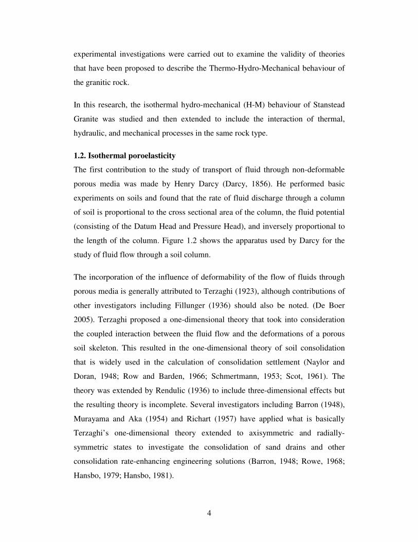
4

experimental investigations were carried out to examine the validity of theories

that have been proposed to describe the Thermo-Hydro-Mechanical behaviour of

the granitic rock.

In this research, the isothermal hydro-mechanical (H-M) behaviour of Stanstead

Granite was studied and then extended to include the interaction of thermal,

hydraulic, and mechanical processes in the same rock type.

1.2. Isothermal poroelasticity

The first contribution to the study of transport of fluid through non-deformable

porous media was made by Henry Darcy (Darcy, 1856). He performed basic

experiments on soils and found that the rate of fluid discharge through a column

of soil is proportional to the cross sectional area of the column, the fluid potential

(consisting of the Datum Head and Pressure Head), and inversely proportional to

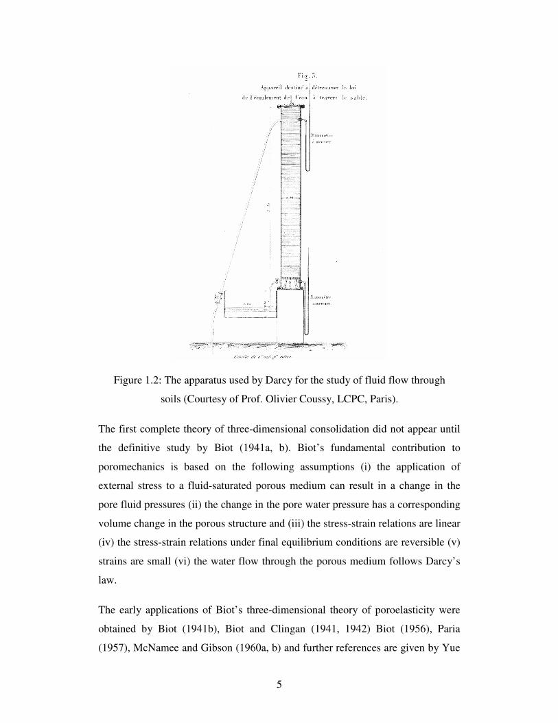
the length of the column. Figure 1.2 shows the apparatus used by Darcy for the

study of fluid flow through a soil column.

The incorporation of the influence of deformability of the flow of fluids through

porous media is generally attributed to Terzaghi (1923), although contributions of

other investigators including Fillunger (1936) should also be noted. (De Boer

2005). Terzaghi proposed a one-dimensional theory that took into consideration

the coupled interaction between the fluid flow and the deformations of a porous

soil skeleton. This resulted in the one-dimensional theory of soil consolidation

that is widely used in the calculation of consolidation settlement (Naylor and

Doran, 1948; Row and Barden, 1966; Schmertmann, 1953; Scot, 1961). The

theory was extended by Rendulic (1936) to include three-dimensional effects but

the resulting theory is incomplete. Several investigators including Barron (1948),

Murayama and Aka (1954) and Richart (1957) have applied what is basically

Terzaghi’s one-dimensional theory extended to axisymmetric and radially-

symmetric states to investigate the consolidation of sand drains and other

consolidation rate-enhancing engineering solutions (Barron, 1948; Rowe, 1968;

Hansbo, 1979; Hansbo, 1981).

5

Figure 1.2: The apparatus used by Darcy for the study of fluid flow through

soils (Courtesy of Prof. Olivier Coussy, LCPC, Paris).

The first complete theory of three-dimensional consolidation did not appear until

the definitive study by Biot (1941a, b). Biot’s fundamental contribution to

poromechanics is based on the following assumptions (i) the application of

external stress to a fluid-saturated porous medium can result in a change in the

pore fluid pressures (ii) the change in the pore water pressure has a corresponding

volume change in the porous structure and (iii) the stress-strain relations are linear

(iv) the stress-strain relations under final equilibrium conditions are reversible (v)

strains are small (vi) the water flow through the porous medium follows Darcy’s

law.

The early applications of Biot’s three-dimensional theory of poroelasticity were

obtained by Biot (1941b), Biot and Clingan (1941, 1942) Biot (1956), Paria

(1957), McNamee and Gibson (1960a, b) and further references are given by Yue

6

(1992), Nguyen (1995), Selvadurai (1996a, 2000, 2007) and Selvadurai and

Suvorov (2012).

The first attempt to compare the consolidation theories of Terzaghi and Biot was

made by Cryer (1963) who used both theories to develop a result for the pore

pressure induced at the center of a surface-drained porous sphere by the

application of an isotropic compressive radial traction. Biot’s theory showed that

the pore pressure increases to a value higher than the surface traction, depending

on the Poisson’s ratio, and then decays until the pore pressure is completely

dissipated. The reason for the excessive increase in the pore pressure is that

drainage from the outermost layer of the sphere causes a decrease in the volume

of that layer, which consequently exerts a compressive stress state to inner layers.

Figure 1.3 shows the changes in the pore pressure at the center of the sphere for

three different values of Poisson’s ratio. The vertical axis shows the normalized

pore pressure at the center of the sphere and the horizontal axis is a dimensionless

time factor, T , defined as

2vC t

Ta

= (1.1)

where vC is the coefficient of consolidation, t is the elapsed time, and a is the

radius of the sphere.

Cryer (1963) showed that since Terzaghi’s theory does not couple the pore

pressure and skeletal deformations it fails to predict the pore pressure rise at the

early stages of the consolidation. The effect was observed earlier by Mandel

(1953) in an experiment involving the compression induced consolidation of a

rectangular region under a plane strain deformation due to a uniaxial load. The

observation related to the pore pressure rise is referred to as the Mandel-Cryer

effect. Thereafter, the effect was investigated by a number of researchers,

including Verruijt (1965), de de Josselin de Jong and Verruijt (1965), Schiffman

7

et al. (1969), Sills (1975), Gibson et al. (1963, 1989), Mason et al. (1991),

Selvadurai and Shirazi (2004) and Selvadurai and Suvorov (2012).

Figure 1.3: Changes in the pore pressure with time in the center of a sphere

subjected to compressive surface traction (reproduced after Gibson et al.,

1963).

The Biot’s theory of poroelasticity, also known as theory of linear poroelasticity,

is well documented in the literature and alternative expositions and

representations are presented in a number of key articles including Rice and

Cleary (1976), Detournay and Cheng (1993), Coussy (1995), Lewis and Schrefler

(1998). Reviews of the subject of isothermal poroelasticity can be found in

Scheidegger (1960), Paria (1963), Selvadurai (1996a, 2007), de Boer (1999),

Wang (2000) and Schanz (2009).

1.3. Permeability

Permeability is the key parameter in the study of poroelastic behavior of

geomaterials under isothermal and non-isothermal conditions. Permeability of a

porous medium is the parameter which governs the rate at which a fluid flows

8

through the pore structure (Harr, 1966; Bear, 1972; Selvadurai et al. 2005). The

permeability of geomaterials can be determined using either steady state or

transient tests depending on the relative values of the anticipated permeability.

Steady state tests are more reliable, since the only measurements needed to

estimate the permeability are the hydraulic potential difference applied to initiate

the fluid flow, the constant flow rate attained and the geometry of the flow

domain. The steady state technique has been used extensively to measure the

permeability of porous media with various geometries and boundary conditions,

including in situ and laboratory tests. Very recently, Selvadurai and Selvadurai

(2010) discussed the steady state patch permeability measurement of an Indiana

Limestone block measuring 508 mm. Their experimental technique for measuring

the near surface permeability of rock used a sealed annular patch. They measured

the near surface permeability of the block and then used inverse analysis

procedures to estimate the permeability characteristics of the interior of the rock.

Selvadurai and Glowacki (2008) examined the hysteresis of permeability in

Indiana Limestone during isotropic loading and unloading. A steady state

technique was used to measure the changes in permeability under confining

pressures that varied between 5 to 60 MPa. They observed a two order of

magnitude decrease in the permeability of the rock at 60 MPa confining pressure,

compared to the permeability measured at a confining pressure of 5 MPa. There

was no recovery of the permeability during the unloading. Heystee and Roegiers

(1980) studied the effect of tensile and compressive stresses on the evolution of

permeability. They developed a radial permeameter to measure the permeability

of rocks under compressive and tensile stresses using the steady state technique.

They tested three different types of rock: Indiana Limestone, red limestone, and

granite. The samples measured 6.4 cm in diameter and 10 cm in length, with a

central co-axial partially drilled cylindrical cavity, measuring 0.64 cm in diameter

and drilled 8.7 cm deep. An increase in permeability was observed under

increasing tensile stresses and a decrease in permeability was noted when the

compressive stress increased. Heiland (2003) performed an exhaustive literature

9

review on the experimental studies performed to determine the evolution of

permeability under different loading and unloading trends associated with

hydrostatic compression, triaxial compression, and uniaxial compression.

For low permeability geomaterials, with permeabilities in the range

K 18 22 2(10 ,10 ) m− −∈ , the accurately verifiable steady flow rates that can be

initiated in unstressed samples without causing damage (e.g. micro-mechanical

hydraulic fracture) to the porous fabric can be small. For this reason, fluid

transport characteristics of low permeability geomaterials are usually determined

from transient flow tests. The use of transient flow tests was pioneered by Brace

et al. (1968). They analyzed the decay of water pressure in a reservoir connected

to one end of a cylindrical Westerly Granite sample. The samples tested measured

1.61 cm in length and 2.5 cm in diameter and were used to study the change of

permeability with depth. In their formulation, they included the compressibility of

the porous skeleton, pore fluid, and solid grains. These compressibilities

contribute to the specific storage of a porous medium. However, for simplicity

they neglected these compressibility values in the analysis of their experimental

results. Lin (1977) discussed the analysis of the transient permeability tests

including the specific storage term, using numerical methods. Bredehoeft and

Papadopulos (1980) discussed the application of a technique for the in situ

measurement of permeability of tight rocks, achieved by pressurizing a finite

length of a shut-in well. They assumed fully radial fluid flow and presented a

mathematical solution for the problem. Hsieh et al. (1981) and Neuzil et al. (1981)

obtained an analytical solution for the piezo-conduction equation. Their method

was able to obtain both the permeability and specific storage term from

experimental data. Trimmer (1982) presented a confining cell similar to that used

by Brace et al (1968) but of a larger size. The experiments focused on the

measurement of the permeability of different low permeability rock types using

samples of dimensions of 15 cm in diameter and 28 cm in height, using steady

state tests for permeabilities higher than 10-17 m2 and the transient technique for

lower permeabilities. Morin and Olsen (1987) suggested using the initial transient

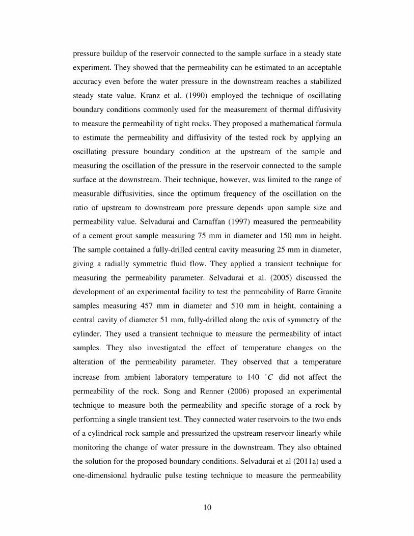
10

pressure buildup of the reservoir connected to the sample surface in a steady state

experiment. They showed that the permeability can be estimated to an acceptable

accuracy even before the water pressure in the downstream reaches a stabilized

steady state value. Kranz et al. (1990) employed the technique of oscillating

boundary conditions commonly used for the measurement of thermal diffusivity

to measure the permeability of tight rocks. They proposed a mathematical formula

to estimate the permeability and diffusivity of the tested rock by applying an

oscillating pressure boundary condition at the upstream of the sample and

measuring the oscillation of the pressure in the reservoir connected to the sample

surface at the downstream. Their technique, however, was limited to the range of

measurable diffusivities, since the optimum frequency of the oscillation on the

ratio of upstream to downstream pore pressure depends upon sample size and

permeability value. Selvadurai and Carnaffan (1997) measured the permeability

of a cement grout sample measuring 75 mm in diameter and 150 mm in height.

The sample contained a fully-drilled central cavity measuring 25 mm in diameter,

giving a radially symmetric fluid flow. They applied a transient technique for

measuring the permeability parameter. Selvadurai et al. (2005) discussed the

development of an experimental facility to test the permeability of Barre Granite

samples measuring 457 mm in diameter and 510 mm in height, containing a

central cavity of diameter 51 mm, fully-drilled along the axis of symmetry of the

cylinder. They used a transient technique to measure the permeability of intact

samples. They also investigated the effect of temperature changes on the

alteration of the permeability parameter. They observed that a temperature

increase from ambient laboratory temperature to 140 Co did not affect the

permeability of the rock. Song and Renner (2006) proposed an experimental

technique to measure both the permeability and specific storage of a rock by

performing a single transient test. They connected water reservoirs to the two ends

of a cylindrical rock sample and pressurized the upstream reservoir linearly while

monitoring the change of water pressure in the downstream. They also obtained

the solution for the proposed boundary conditions. Selvadurai et al (2011a) used a

one-dimensional hydraulic pulse testing technique to measure the permeability

11

hysteresis of the Cobourg Limestone under isotropic compressive loading and

unloading ranging from 5 to 20 MPa. Two samples measuring 100 mm in

diameter and 200 mm in height were tested. Unlike similar tests performed on

homogenous rock types, the Cobourg Limestone tested showed a permeability

increase both in loading and unloading. The micromechanical damage or cracking

at the inter-nodular boundaries due to the inhomogeneity of the material was

associated with this observation. Selvadurai and Jenner (2013) examined the

permeability of the same rock type under unconfined conditions. Four samples

were tested using steady state and transient techniques. The samples measured

107 mm in diameter and 117 to 174 mm in height; they all contained a central

cavity 13 mm in diameter. Radial flow was established along the bedding plane of

the rock. The measured permeability ranged within three orders of magnitude.

Selvadurai (2009) theoretically studied the influence of residual pore pressure

gradients on decay curves for one-dimensional transient tests. The residual pore

pressure can be due to a saturation process either under negative pressure or under

a steady state flow that was induced prior to the transient test.

All experimental and computational studies mentioned above used transient fluid

flow formulations that weakly take into account the effect of skeletal

deformations through the incorporation of storativity terms. However, neglecting

the poroelastic coupling between the pore water and porous skeleton can

introduce errors in the estimation of permeability from transient tests. Walder and

Nur (1986) examined the effect of poroelastic phenomena on the interpretation of

pressure pulse decay curves in transient tests. They assumed that short samples

had a state of constant strain while long samples were in a state of constant stress

and showed that the hydraulic diffusivity for these two cases are size dependent

and, therefore, one should expect a size dependency in the interpretation of the

permeability from hydraulic pulse test results. They also performed some

experiments to further investigate their claim; transient tests were conducted on

several samples measuring 5.1 cm in diameter, with lengths varying from 21.7

mm to 47.6 mm. However, the effect was not clearly observed in the experiments.

The variability in material properties from core to core was explained as the

12

probable reason that masked the influence of sample size dependency. Adachi and

Detournay (1997) modified the formulation proposed by Kranz et al. (1990) for

the oscillating pore pressure method used in the transient measurement of

permeability. They analytically solved the coupled poroelastic problem of a very

slender specimen tested for permeability using a pore pressure oscillation

technique. The possible influences of the two approaches for examining the

results of hydraulic pulse tests on the interpretation of permeability values have

lead to comparative investigations and two examples are provided by Walder and

Nur (1986) and Hart and Wang (1998) (see also Wang, 2000). Both investigations

deal with hydraulic pulse tests conducted under one-dimensional conditions with

the first investigating the poroelastic phenomena including non-linear pore

pressure diffusion associated with large pore pressure gradients while the latter

considers the three-dimensional poroelastic influences that arise when modelling

the one-dimensional hydraulic pulse tests. It should also be noted that the problem

examined by Hart and Wang (1998) relates to the computational modelling of the

propagation of a hydraulic pulse on a one-dimensional element that is

hydraulically sealed at all surfaces other than at the region subjected to pressure.

1.4. Non-isothermal Poroelasticity

The classical theory of poroelasticity, proposed by Biot (1941a), is restricted to

isothermal processes in geomechanics of fluid-saturated media. In a variety of

problems associated with deep geological disposal of nuclear wastes, oil and

natural gas recovery and geothermal energy extraction, the processes encountered

are non-isothermal. Biot’s isothermal theory of linear poroelasticity can be

extended for including effects of temperature on the hydro-mechanical behavior

of porous media.

The first attempts to formulate the coupled thermo-hydro-mechanical behavior of

mixtures of porous and fluid media were presented by Brownell et al. (1977) and

Morland (1978). In these studies the deformations of the porous solid are

represented by approximate mixture formulations that do not reduce to the Navier

equations applicable to a porous solid. Noorishad et al. (1984) used a finite

13

element approach to examine the coupled thermo-hydro-mechanical phenomena

in saturated fractured rocks, investigating the fracture inflow near a heater.

Booker and Savvidou (1984, 1985) performed analytical studies of the thermo-

elastic consolidation of a saturated soil containing a buried point heat source and a

spherical heat source. They obtained the changes of pore pressure and stresses

around the heat source with time. Savvidou and Booker (1988) later obtained the

analytical solution for a spherical heat source with a decaying power output,

located in a saturated infinite porous medium. Aboustit et al. (1985) developed a

variational approach based on the results of Gurtin (1966) to examine the thermo-

elastic consolidation of porous media. The solid matrix was assumed to be linear

elastic and the fluid was assumed to be incompressible. McTigue (1986) proposed

a coupled thermo-hydro-mechanical formulation which was an extention of the

Biot’s isothermal theory of linear poroelasticity. The formulation accounted for

the compressibility of the fluid, the deformability of the porous skeleton, and the

solid constituents. Coussy (1989) developed a formulation for thermo-poro-elasto-

plasticity. He derived the equations from the thermodynamics of open systems

and irreversible processes. Selvadurai and Nguyen (1995) presented a

comprehensive development of the equations governing a fluid-saturated porous

medium with compressible grains and compressible fluid. The heat conduction in

the porous medium is represented by the uncoupled formulation which implies

that neither the deformations nor the fluid flow will generate heating. Nguyen and

Selvadurai (1995) also applied this development to examine pore pressure

generation due to heating of a cementitious material. Rehbinder (1995) obtained

an analytical solution for the stationary coupled thermo-hydro-mechanical

problem of a spherical or a cylindrical heat source in an infinite medium,

imposing simplifications to the physical process. These results provided a

benchmark solution to be used for the validation of finite element codes. Zhou et

al. (1998), also presented coupled thermo-hydro-mechanical formulation, based

on Biot’s isothermal poroelastic equations. They obtained the Laplace transform

domain solutions for spherical and cylindrical cavities embedded in homogeneous

and non-homogeneous infinite media, subjected to a temperature increase on the

14

cavity surface for simplified cases and used numerical techniques for Laplace

transform inversion. It was observed that for low permeability geomaterials, the

thermodynamically coupled heat and water flow has a negligible effect on heat

flow. Also, the effects of mechanical deformation and pore pressure change on

temperature change can be neglected, and thus the temperature distribution can be

fully uncoupled from pore pressure and skeletal deformations which were implicit

in the development of Selvadurai and Nguyen (1995). Gens et al. (1998) analyzed

the thermo-hydro-mechanical measurements of a full scale in situ test, carried out

in the granitic rock in the underground laboratory at Grimsel, Switzerland. The

test, referred to as the FEBEX experiment, used heaters emplaced in steel

canisters to model the heat emitted by the decaying nuclear wastes and employed

a finite element code to implement their THM formulation. Pao et al. (2001)

obtained a fully coupled THM model for a three phase porous medium containing

water, gas, and heavy crude oil. Suvorov and Selvadurai (2010) obtained

macroscopic constitutive equations of thermo-poro-visco-elasticity using

eigenstrains, and examined the one-dimensional response under temperature

change and undrained conditions. Comparisons were provided between thee

computational model (ABAQUSTM) and the analytical results. Chen et al. (2009)

presented the equations to model the THM behaviour of unsaturated porous

media. They took into account the six different processes of stress-strain, water

flow, gas flow, vapour flow, heat transport, and porosity evolution in their model.

They also accounted for the phase transition and gas solubility in liquid. The

implementation of the model required knowledge of 16 physical and mechanical

parameters. The equations were solved using the finite element technique and

validated the results against two existing laboratory and in situ measurements.

Belotserkovets and Prevost (2011) performed an analytical study of the thermo-

poro-elastic response of a fluid-saturated porous sphere to a surface compressive

traction, similar to that which was assumed for the Mandel-Cryer problem. They

observed that the maximum temperature increase due to a surface mechanical

stress of 1 GPa for an arbitrary sphere of rock with a radius of 4 m was less than

3% of the ambient temperature. Selvadurai and Suvorov (2012) examined the

15

problem of the boundary heating of poroelastic and poroelasto-plastic spheres.

The governing equations were similar to those developed by Selvadurai and

Nguyen (1995) for THM behavior of a poroelastic material. The analytical results

for the poroelastic case displays the THM Mandel-Cryer effect and the

computational results elaborate how elasto-plasticity can moderate the generation

of pore pressure at the center of the sphere.

In addition to above studies, exhaustive research is underway to study the

different geo-environmental aspects of geological disposal of spent nuclear fuel,

under the auspices of the DECOVALEX project (DEvelopment of COupled

Models and their VALidation against EXperiments in Nuclear Waste Isolation).

The project group consists of five international research teams. Examples of the

results of their collaboration are summarized in the articles by: Rutqvist et al.

(2001), Chijimatsu et al. (2005), Millard et al. (2005), Rutqvist et al. (2005),

Nguyen et al. (2009), Wang et al. (2011). Their investigations included a

comparison of different formulations to model the coupled unsaturated thermo-

hydro-mechanical behaviour of the host rock under the thermal loading of nuclear

wastes, for intact and fractured rocks, and also the analysis of large scale in situ

tests performed at various underground research laboratories (URL), in different

countries including Canada, Switzerland, and Japan.

1.5. Objectives and scope of the research

The research presented in this thesis deals with the experimental and

computational study of the Thermo-Hydro-Mechanical behavior of low

permeability geomaterials. The experiments were performed on Stanstead Granite

samples. The granitic rock is found in Eastern Canada, but is similar to the rocks

of Canadian Shield being considered as a host rock for a deep geological

repository for nuclear fuel wastes.

The physical and mechanical characteristics of the rock are examined through a

series of standard experiments and the results are compared with similar values in

the literature.

16

The application of Biot’s theory of isothermal linear poroelasticity is discussed

along with the limiting case where the stress field decouples from the fluid flow

equation leading to the conventional piezo-conduction equation for the pressure

decay. The effect of the compressibility of the porous skeleton, the solid grains

and the permeating fluid on the hydro-mechanical behavior of geomaterials is also

studied.

The permeability of the granitic rock was measured using steady state and

hydraulic pulse testing techniques and over various one-dimensional and radially

symmetric geometries and boundary conditions. The range of applicability of the

piezo-conduction equation, which is used as a procedure for determining the

hydraulic properties of rocks, is examined using alternative theoretical

formulations. The influence of both free-air and dissolved air in the pressurized

cavity that is used in the hydraulic pulse tests is also studied and a computational

technique is proposed to minimize their effect on the estimation of permeability

from experimental results.

Since the pressure of overburden in situ can affect the permeability characteristics

of the rock, the change of permeability in Stanstead Granite was studied under

isotropic loading and unloading using the technique developed by Selvadurai and

Glowacki (2008).

The non-isothermal application of Biot’s theory of poroelasticity is discussed. A

testing facility was designed and fabricated in order to examine the thermo-hydro-

mechanical behavior of low permeability geomaterials. Two samples of Stanstead

Granite were tested to study the coupling effects of skeletal deformations, pore

pressure and temperature changes on Stanstead Granite.

The finite element code of COMSOL MultiphysicsTM was used throughout this

research to develop computational results for isothermal and non-isothermal

poroelastic theories.

17

CHAPTER 2

MECHANICAL AND PHYSICAL CHARACTERIZATION OF THE STANSTEAD GRANITE

2.1. General description

Stanstead Granite is a medium gray, medium to coarse-grained rock, recovered

from the Beebe region of the Eastern Townships in Quebec, Canada. The minerals

are clear, sharply defined quartz (2.5 to 5 mm); feldspar laths (2 to 3 mm), which

are semi transparent to milky white; muscovite flakes (0.5 mm), in small amounts;

sharply contrasting biotite in flakes and clusters (3 mm) and some chlorite flakes

(to 1mm) . The grains are subhedral and give an interlocking granular fabric

(Appendix A). The samples of Stanstead Granite used in this research showed no

visual evidence of stratifications that could lead to anisotropic or transversely-

isotopic estimates of properties.

A series of tests were performed to characterize the chemical composition, and

physical and mechanical properties of the rock. These tests included X-ray

fluorescence spectrometry (XRF), conventional saturation porosity measurement,

mercury intrusion porosimetry (ASTM, D4404-84) and a uniaxial compression

test (ASTM D7012-04) to measure Young’s modulus, Poisson’s ratio, and the

uniaxial compressive strength of Stanstead Granite. In addition, Brazilian Tests

18

(ASTM D3967-08) were used to estimate the tensile strength of Stanstead

Granite.

2.2. Chemical composition

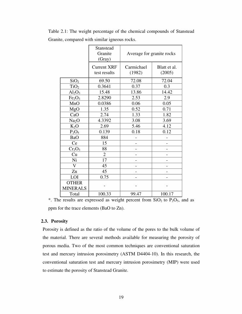
The X-ray Fluorescence Spectrometry (XRF) method was used to characterize the

chemical composition of Stanstead Granite. The technique relies on the response

of atoms to X-ray excitations. X-rays are electro-magnetic short wavelength

radiation with high energy and high frequency. Excitation of minerals with X-ray

radiation ionizes them. The X-ray radiation, if powerful enough, can dislodge an

electron from an inner shell of an atom that will be replaced by an outer shell

electron. This process emits energy since an inner shell electron has a stronger

bound than an outer bound electron; the emitted energy is in the form of

fluorescent radiation. Since the energy difference between the electron shells are

fixed and known, an analysis of the emitted fluorescence radiation can be used to

characterize the elements contained in a sample (Shackley, 2011).

An XRF test of Stanstead Granite was performed in the Earth and Planetary

Sciences Department of McGill University. The weight percentage of the major

elements is shown in Table 2.1 and compared to similar results from the literature.

Analyzes were performed on fused beads prepared from ignited samples. It can be

seen that silicon (Si) and aluminum (Al) are the two major elements in Stanstead

Granite and igneous rocks, in general. These elements form the minerals of the

rock.

19

Table 2.1: The weight percentage of the chemical compounds of Stanstead

Granite, compared with similar igneous rocks.

Stanstead Granite (Gray)

Average for granite rocks

Current XRF

test results Carmichael

(1982) Blatt et al.

(2005)

SiO2 69.50 72.08 72.04 TiO2 0.3641 0.37 0.3 Al2O3 15.48 13.86 14.42 Fe2O3 2.8290 2.53 2.9 MnO 0.0386 0.06 0.05 MgO 1.35 0.52 0.71 CaO 2.74 1.33 1.82 Na2O 4.3392 3.08 3.69 K2O 2.69 5.46 4.12 P2O5 0.139 0.18 0.12 BaO 884 - - Ce 15 - -

Cr2O3 88 - - Cu 2 - - Ni 17 - - V 45 - - Zn 45 - -

LOI 0.75 - - OTHER

MINERALS - - -

Total 100.33 99.47 100.17 *. The results are expressed as weight percent from SiO2 to P2O5, and as

ppm for the trace elements (BaO to Zn).

2.3. Porosity

Porosity is defined as the ratio of the volume of the pores to the bulk volume of

the material. There are several methods available for measuring the porosity of

porous media. Two of the most common techniques are conventional saturation

test and mercury intrusion porosimetry (ASTM D4404-10). In this research, the

conventional saturation test and mercury intrusion porosimetry (MIP) were used

to estimate the porosity of Stanstead Granite.

20

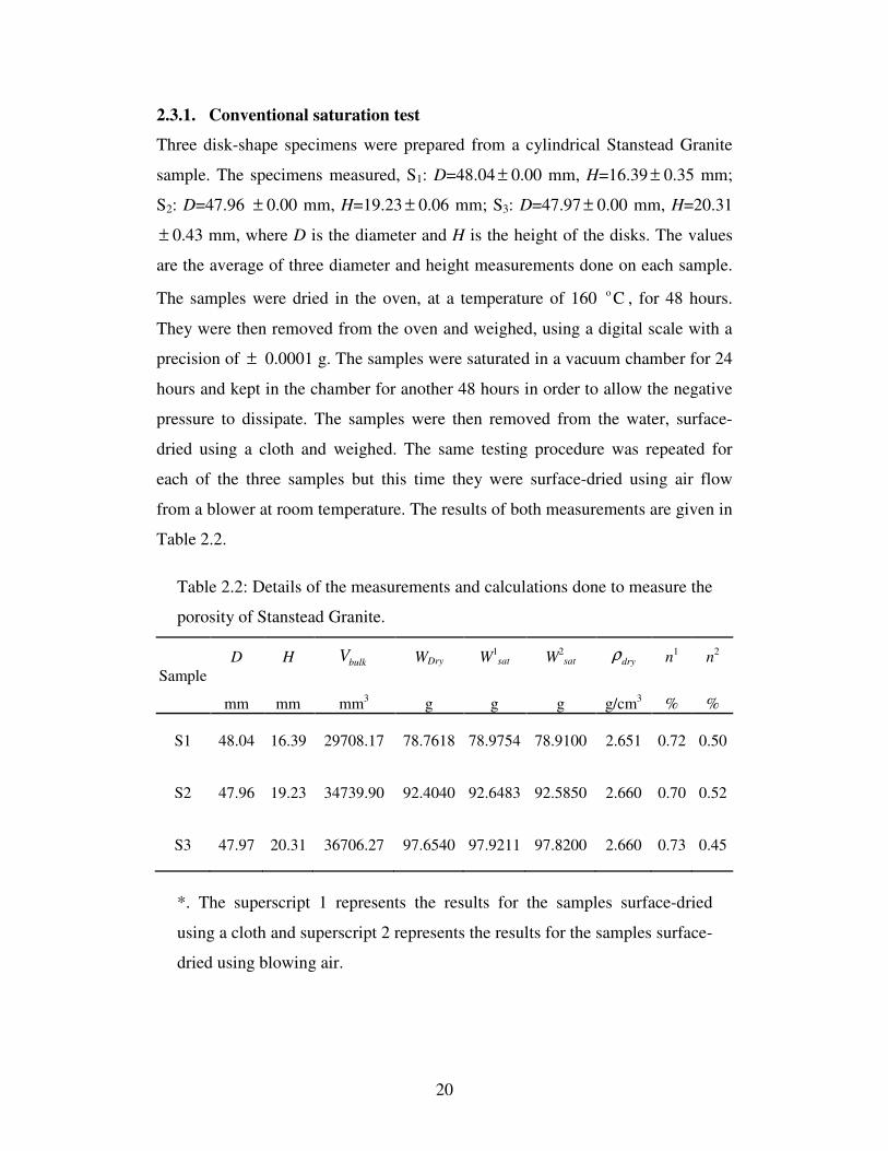
2.3.1. Conventional saturation test

Three disk-shape specimens were prepared from a cylindrical Stanstead Granite

sample. The specimens measured, S1: D=48.04 ± 0.00 mm, H=16.39 ± 0.35 mm;

S2: D=47.96 ± 0.00 mm, H=19.23 ± 0.06 mm; S3: D=47.97 ± 0.00 mm, H=20.31

± 0.43 mm, where D is the diameter and H is the height of the disks. The values

are the average of three diameter and height measurements done on each sample.

The samples were dried in the oven, at a temperature of 160 o C , for 48 hours.

They were then removed from the oven and weighed, using a digital scale with a

precision of ± 0.0001 g. The samples were saturated in a vacuum chamber for 24

hours and kept in the chamber for another 48 hours in order to allow the negative

pressure to dissipate. The samples were then removed from the water, surface-

dried using a cloth and weighed. The same testing procedure was repeated for

each of the three samples but this time they were surface-dried using air flow

from a blower at room temperature. The results of both measurements are given in

Table 2.2.

Table 2.2: Details of the measurements and calculations done to measure the

porosity of Stanstead Granite.

Sample D

H

bulkV

WDry

W

1sat

W2

sat

dryρ

n1

n2

mm mm mm3 g g g g/cm3 % %

S1 48.04 16.39 29708.17 78.7618 78.9754 78.9100 2.651 0.72 0.50

S2 47.96 19.23 34739.90 92.4040 92.6483 92.5850 2.660 0.70 0.52

S3 47.97 20.31 36706.27 97.6540 97.9211 97.8200 2.660 0.73 0.45

*. The superscript 1 represents the results for the samples surface-dried

using a cloth and superscript 2 represents the results for the samples surface-

dried using blowing air.

21

The average porosity of the rock was measured as 0.7% for the samples surface-

dried using a cloth and 0.5%, for the samples surface-dried using blowing air. The

blowing air dries the sample to a greater depth, compared to using a cloth to dry

the surface; therefore, a lower porosity value is obtained. Also, using the above

results, the bulk density of the dry sample was calculated to be 2.65 g/cm3.

2.3.2. Mercury intrusion porosimetry

Mercury intrusion porosimetry (MIP) has proved to be a useful technique in

measuring the porosity of porous materials, specially those with low porosity. The

technique was first proposed by Washburn (1921). Ritter and Drake (1945) built

the first MIP testing apparatus, which was able to inject mercury into pores with a

diameter of less than 2 nm.

The parameters that can be measured using the MIP technique are the total pore

volume, pore size distribution, density of solids and powders, and the specific

surface area of pores (Aligizaki, 2006). Mercury is chosen as the intruding fluid

since it has low vapour pressure, it is inert in terms of chemical reactivity with

many materials, and has non-wetting properties for most surfaces. Because of the

non-wetting property of mercury, if a porous specimen is immersed in mercury at

atmospheric temperature, the mercury does not intrude into the pores. A liquid

can wet a solid surface if the attraction between the solid and the liquid molecules

is greater than the attraction of liquid molecules to each other. For comparison,

the contact angle between water and many surfaces is between 20o to 30o while

for mercury it is usually greater than 90o (Aligizaki, 2006).

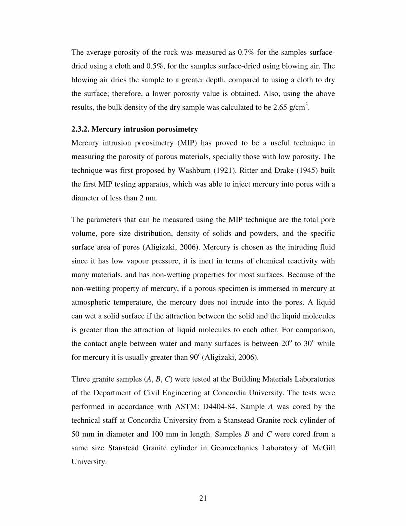
Three granite samples (A, B, C) were tested at the Building Materials Laboratories

of the Department of Civil Engineering at Concordia University. The tests were

performed in accordance with ASTM: D4404-84. Sample A was cored by the

technical staff at Concordia University from a Stanstead Granite rock cylinder of

50 mm in diameter and 100 mm in length. Samples B and C were cored from a

same size Stanstead Granite cylinder in Geomechanics Laboratory of McGill

University.

22

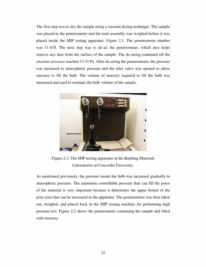
The first step was to dry the sample using a vacuum drying technique. The sample

was placed in the penetrometer and the total assembly was weighed before it was

placed inside the MIP testing apparatus, Figure 2.1. The penetrometer number

was 11-878. The next step was to de-air the penetrometer, which also helps

remove any dust from the surface of the sample. The de-airing continued till the

absolute pressure reached 13.33 Pa. After de-airing the penetrometer, the pressure

was increased to atmospheric pressure and the inlet valve was opened to allow

mercury to fill the bulb. The volume of mercury required to fill the bulb was

measured and used to estimate the bulk volume of the sample.

Figure 2.1: The MIP testing apparatus at the Building Materials

Laboratories at Concordia University.

As mentioned previously, the pressure inside the bulb was increased gradually to

atmospheric pressure. The minimum controllable pressure that can fill the pores

of the material is very important because it determines the upper bound of the

pore sizes that can be measured in the apparatus. The penetrometer was then taken

out, weighed, and placed back in the MIP testing machine for performing high

pressure test. Figure 2.2 shows the penetrometer containing the sample and filled

with mercury.

23

Figure 2.2: The penetrometer with a bulb that is filled with mercury at the

end of the low pressure range test.

Pressure was increased incrementally in this step to 4000 atm, which corresponds

to a pore diameter of 2 nm. After each pressure step increase, the system was

allowed to equilibrate.

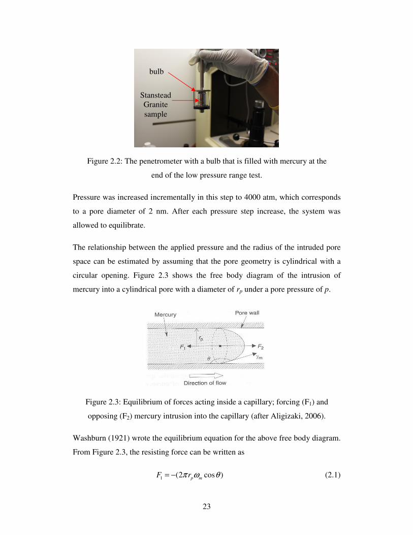
The relationship between the applied pressure and the radius of the intruded pore

space can be estimated by assuming that the pore geometry is cylindrical with a

circular opening. Figure 2.3 shows the free body diagram of the intrusion of

mercury into a cylindrical pore with a diameter of rp under a pore pressure of p.

Figure 2.3: Equilibrium of forces acting inside a capillary; forcing (F1) and

opposing (F2) mercury intrusion into the capillary (after Aligizaki, 2006).

Washburn (1921) wrote the equilibrium equation for the above free body diagram.

From Figure 2.3, the resisting force can be written as

1 (2 cos )p m

F rπ ω θ= − (2.1)

bulb

Stanstead Granite sample

24

where m

ω is the surface tension between the inner wall of the cylinder and

mercury and θ is the contact angle between mercury and the solid surface.

Also, the driving force can be written as

22 ( )pF r pπ= (2.2)

Given that the above driving and resisting forces should be equal under quasi-

static conditions, the radius of the intruded force under the pore pressure p can be

calculated

2 cosm

pr

p

ω θ−= (2.3)

where, rp is the pore radius.

Rootare and Prenzlow (1967) derived an equation to estimate the surface porosity

of a porous material, using the measured pressure change versus intruded volume

of mercury. The equation can be written for a simplified cylindrical pore

geometry (Aligizaki, 2006). The work required to increase the surface area of a

cylindrical pore wetted by mercury is

1 cosm

dW dSω θ= − (2.4)

where dS is the surface area of the pore wetted by mercury. The work required for

driving mercury into the pore is

2dW pdV= (2.5)

where dV is the increment of the volume of mercury intruded into the pore by

applying a pore pressure, i.e. p. Assuming that the intrusion of mercury in pores is

reversible and thus no heat is produced in the process, the above two equations

can be equated and the surface area of the wetted pore can be calculated

25

cosm

pdVdS

ω θ= (2.6)

Integrating from both sides of the above equation gives the total surface area of

the material wetted by mercury

0

1

cos

V

m

S pdVω θ

= ∫ (2.7)

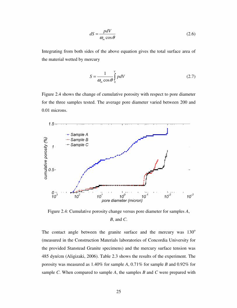
Figure 2.4 shows the change of cumulative porosity with respect to pore diameter

for the three samples tested. The average pore diameter varied between 200 and

0.01 microns.

Figure 2.4: Cumulative porosity change versus pore diameter for samples A,

B, and C.

The contact angle between the granite surface and the mercury was 130o

(measured in the Construction Materials laboratories of Concordia University for

the provided Stanstead Granite specimens) and the mercury surface tension was

485 dyn/cm (Aligizaki, 2006). Table 2.3 shows the results of the experiment. The

porosity was measured as 1.40% for sample A, 0.71% for sample B and 0.92% for

sample C. When compared to sample A, the samples B and C were prepared with

26

more attention at Geomechanics Laboratory of McGill University, resulting in

less damage during the preparation phase. This would explain the slight

discrepancy between the measured results of porosity for sample A when

compared to samples B and C. It should be noted that the mercury intrusion

porosimetry technique measures the total porosity, where it is composed of both

connected and non-connected pores. Therefore, compared to the conventional

saturation technique, the MIP result gives an upper bound for the porosity of a

porous geomaterial.

Table 2.3: Experimental results of MIP tests performed on three samples of

Stanstead Granite.

Sample Dry Weight

(g)

Bulk Volume

(ml)

Bulk density

(g/ml)

Grain density

(g/ml)

Porosity

%

A 7.141 2.7107 2.634 2.671 1.396

B 4.423 1.6743 2.645 2.660 0.713

C 4.150 1.5803 2.634 2.650 0.919

2.4. Elasticity parameters and compressive strength

The Young’s modulus, Poisson’s ratio, and uniaxial compressive strength of

Stanstead Granite were measured and compared with the data available in the

literature. Four uniaxial compression tests were performed on dry cylindrical

samples measured 5 cm in diameter and 10 cm in height. The ASTM standard test

method (ASTM, D7012-04) was used to determine the compressive strength and

elastic moduli of the specimen. The samples were machined to obtain parallel

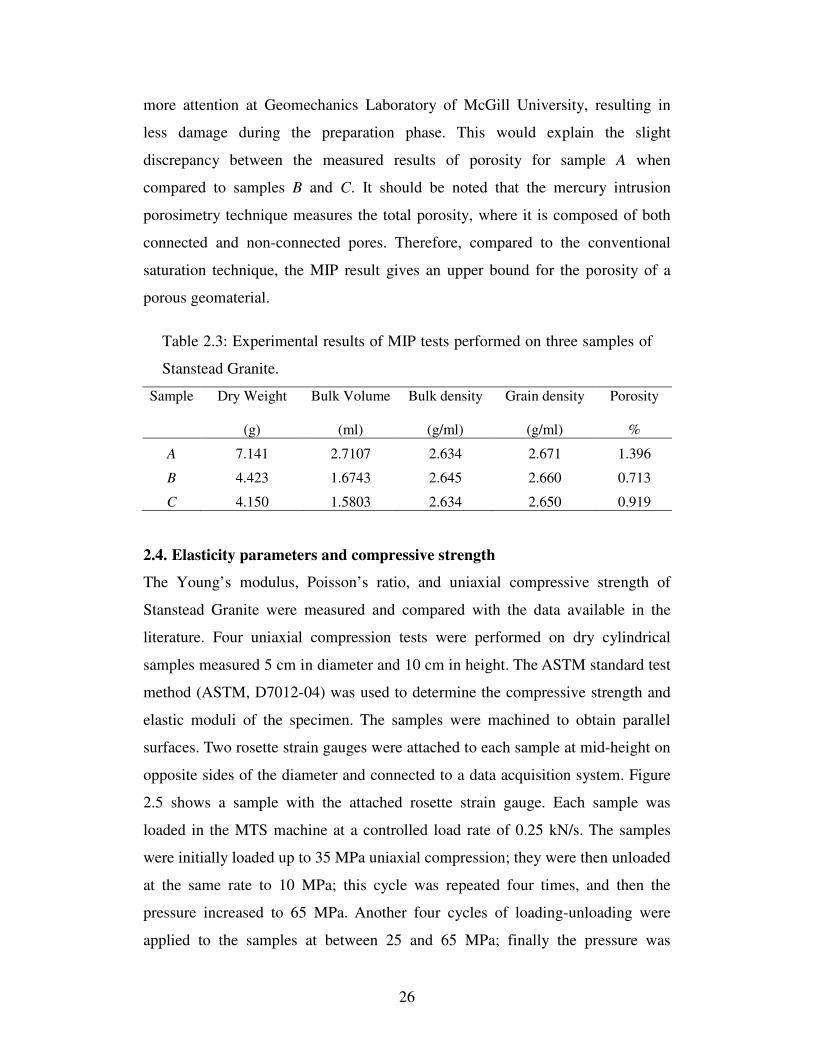
surfaces. Two rosette strain gauges were attached to each sample at mid-height on

opposite sides of the diameter and connected to a data acquisition system. Figure

2.5 shows a sample with the attached rosette strain gauge. Each sample was

loaded in the MTS machine at a controlled load rate of 0.25 kN/s. The samples

were initially loaded up to 35 MPa uniaxial compression; they were then unloaded

at the same rate to 10 MPa; this cycle was repeated four times, and then the

pressure increased to 65 MPa. Another four cycles of loading-unloading were

applied to the samples at between 25 and 65 MPa; finally the pressure was

27

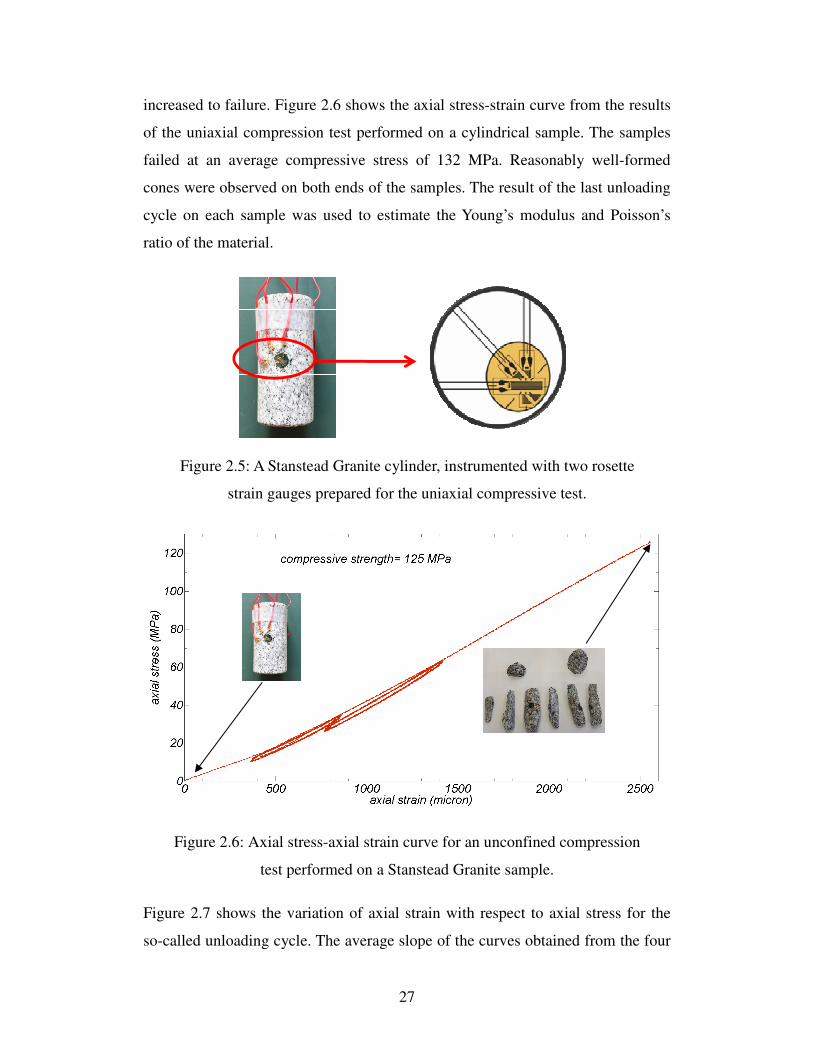
increased to failure. Figure 2.6 shows the axial stress-strain curve from the results

of the uniaxial compression test performed on a cylindrical sample. The samples

failed at an average compressive stress of 132 MPa. Reasonably well-formed

cones were observed on both ends of the samples. The result of the last unloading

cycle on each sample was used to estimate the Young’s modulus and Poisson’s

ratio of the material.

Figure 2.5: A Stanstead Granite cylinder, instrumented with two rosette

strain gauges prepared for the uniaxial compressive test.

Figure 2.6: Axial stress-axial strain curve for an unconfined compression

test performed on a Stanstead Granite sample.

Figure 2.7 shows the variation of axial strain with respect to axial stress for the

so-called unloading cycle. The average slope of the curves obtained from the four

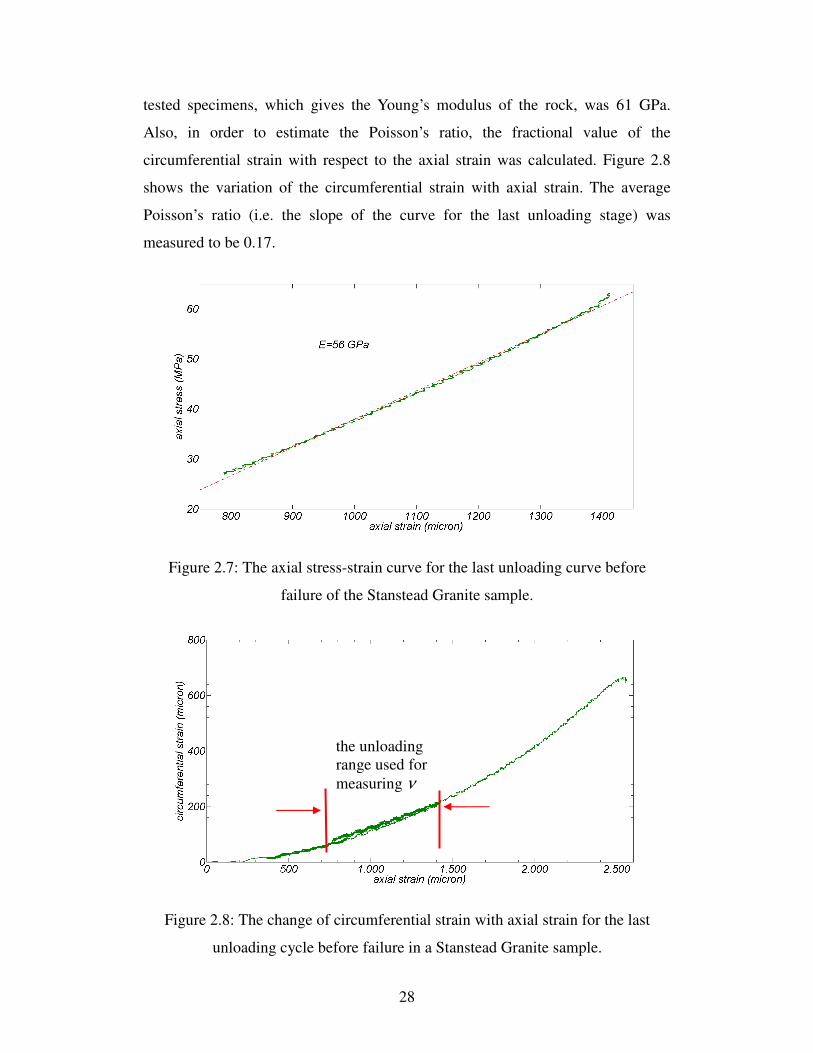
28

tested specimens, which gives the Young’s modulus of the rock, was 61 GPa.

Also, in order to estimate the Poisson’s ratio, the fractional value of the

circumferential strain with respect to the axial strain was calculated. Figure 2.8

shows the variation of the circumferential strain with axial strain. The average

Poisson’s ratio (i.e. the slope of the curve for the last unloading stage) was

measured to be 0.17.

Figure 2.7: The axial stress-strain curve for the last unloading curve before

failure of the Stanstead Granite sample.

Figure 2.8: The change of circumferential strain with axial strain for the last

unloading cycle before failure in a Stanstead Granite sample.

the unloading range used for measuring ν

29

2.5. Tensile strength

The splitting tensile strength of Stanstead Granite was measured by performing a

series of experiments in accordance with ASTM D3967-08. It should be noted

that the tensile strength is obtained by performing direct uniaxial tensile test

(ASTM D2936-08), which is difficult and expensive. Splitting tensile test

(Brazilian test) on the other hand is easy to perform and inexpensive and for this

reason is the common test to examine the tensile strength of rock and concrete

specimens.

Four cylindrical Stanstead Granite samples were tested. The ratio of thickness (t)

to diameter (D) of the samples was between 0.72 to 0.74, which is within the

specified range in the standard (0.2 to 0.75). The samples were cored from a

Stanstead Granite slab and the thicknesses were reduced to comply with the above

mentioned t/D specification using a diamond saw. The dimensions of the samples

are shown in Table 2.4. Each dimension is the average of four measurements.

Figure 2.9 shows the testing apparatus. The samples were tested in an MTS

315.03 Load Frame with the capacity of 4500 kN. In order to avoid high stress

concentration and local damage, plywood strips with the thickness of 4 mm were

placed between the loading platens and the sample at the top and bottom contact

areas. The samples were loaded at a constant displacement rate of 0.5 mm/min to

failure. A 450 kN StrainsertTM load cell was used to measure the applied load.

The splitting tensile strength was calculated using the following equation (ASTM

D3967-08)

2

t

P

tDσ

π= (2.8)

where t

σ is the splitting tensile strength, P is the failure load, t is the thickness of

the specimen, and D is the diameter of the specimen. The splitting tensile strength

of the tested Stanstead Granite specimens ranged between (7.9 to 8.8) MPa with

the average value of 8.4 MPa.

30

Table 2.4: The result of the splitting tensile strength tests performed on four

samples of Stanstead Granite.

Sample Height

(mm)

Diameter

(mm) t/D

Loading Rate

(mm/min)

Failure Load

(kN)

Splitting tensile

strength (MPa)

BT-1 79.58 107.11 0.74 0.5 115 8.6

BT-2 77.83 106.78 0.73 0.5 102 7.8

BT-3 77.22 106.24 0.73 0.5 110 8.5

BT-4 76.03 105.58 0.72 0.5 111 8.8

Figure 2.9: The testing assembly used for performing Brazilian tensile

strength tests (the assembly is shown from two different angles).

2.6. Summary

Stanstead Granite is a medium gray, medium to coarse grained rock with crystal

sizes ranging from 0.5 mm to 5 mm. The main minerals in Stanstead Granite are

quartz, plagioclase, potassium feldspar, biotite and epidote. The porosity of the

rock was measured using a classic saturation technique and mercury intrusion

porosimetry (MIP). Using a standard saturation technique, the porosity was found

to be in the range of 0.5% to 0.7%, while the MIP technique measured the

31

porosity in the range of 0.7% to 1.4%. Along with porosity measurements, the dry

density of the material was also measured. Table 2.5 shows the results of the

measurements compared to results of similar experiments performed on granitic

rocks. The bulk dry density of the rock was (2630 to 2660) kg/m3 and the grain

density was in the range of (2650 to 2670) kg/m3.

Table 2.5: The measured physical parameters compared to similar values

available in the literature.

Rock type

Porosity

%

Bulk Density

(kg/m3)

Grain Density

(kg/m3)

Saturation MIP

Stanstead Granite

(Current Study) (0.45-0.73)3 (0.71-1.40)3 (2630-2660)* (2650-2670)*

Stanstead Granite

(Iqbal and Mohanty, 2007) 0.623 - 26503 -

Barre Granite

(Selvadurai et al., 2005) 1.01 - 2630 2660

Barre Granite


Laurentian Granite


• The subscripts denote the number of samples tested for each parameter.

• The values with an asterisk are the results of three samples tested using the saturation technique and three samples tested with MIP technique.

The mechanical properties of Stanstead Granite were also measured by

performing 4 unconfined compression tests and four splitting tensile strength

tests. The uniaxial compressive strength of the samples was measured as 132

MPa. The Young’s modulus and the Poisson’s ratio were measured as 61 GPa and

0.17, respectively. The splitting tensile strength of Stanstead Granite was also

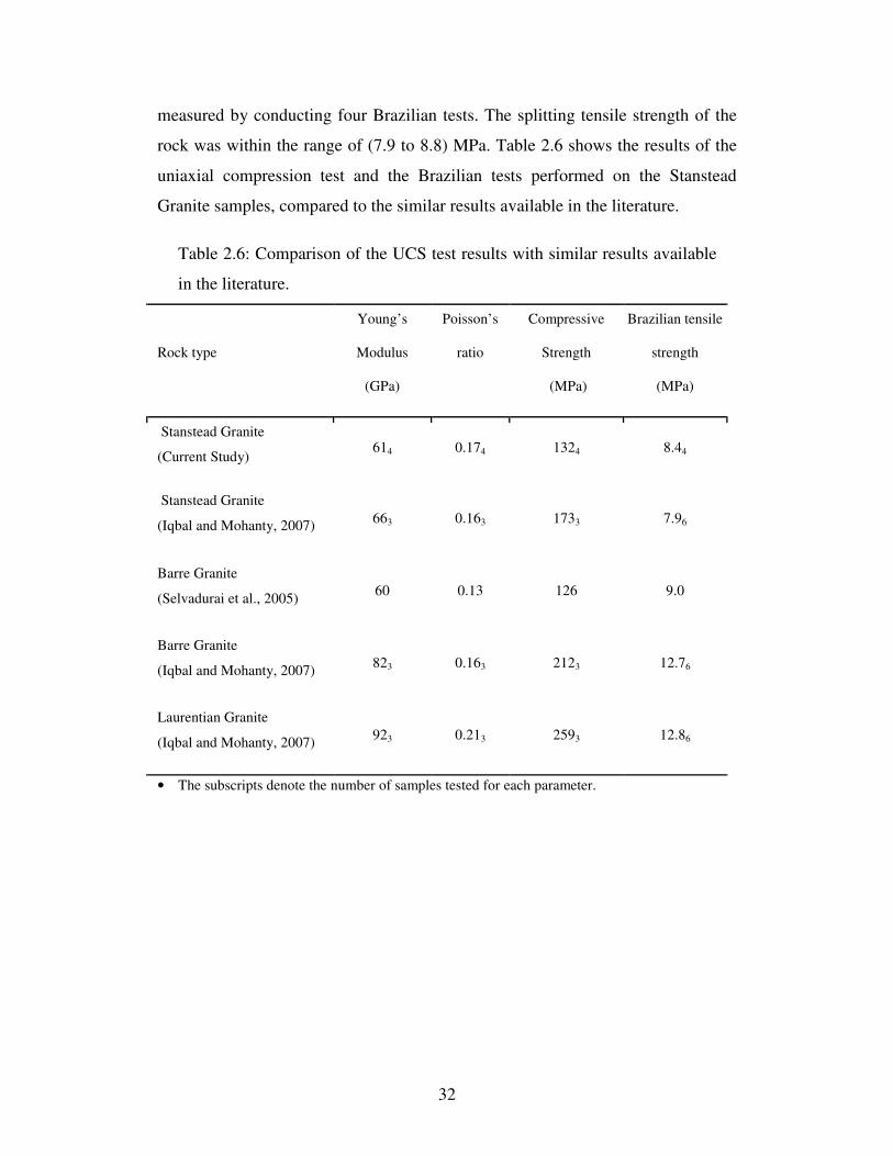
32

measured by conducting four Brazilian tests. The splitting tensile strength of the

rock was within the range of (7.9 to 8.8) MPa. Table 2.6 shows the results of the

uniaxial compression test and the Brazilian tests performed on the Stanstead

Granite samples, compared to the similar results available in the literature.

Table 2.6: Comparison of the UCS test results with similar results available

in the literature.

Rock type

Young’s

Modulus

(GPa)

Poisson’s

ratio

Compressive

Strength

(MPa)

Brazilian tensile

strength

(MPa)

Stanstead Granite

(Current Study) 614 0.174 1324 8.44

Stanstead Granite

(Iqbal and Mohanty, 2007) 663 0.163 1733 7.96

Barre Granite

(Selvadurai et al., 2005) 60 0.13 126 9.0

Barre Granite


Laurentian Granite


• The subscripts denote the number of samples tested for each parameter.

33

CHAPTER 3

ISOTHERMAL BEHAVIOUR OF POROELASTIC MEDIA

3.1. Introduction

This chapter deals with the iso-thermal hydro-mechanical behaviour of linear

elastic porous geomaterials. The mechanical deformation and pore pressure have

coupling effects and the study of these effects are important to several

geomechanical applications, including consolidation of soils (Biot, 1941b; Biot

and Clingan, 1941, 1942), heave and subsidence of the geologic media due to

groundwater discharge or oil withdrawal (Geertsma, 1973; Hsieh, 1996; Burbey,

2008), and hydraulic fracturing (Detournay and Cheng, 1990; Boone and

Detournay, 1990). Although the contributions made by Terzaghi (1923) in the

development of the one-dimensional theory of consolidation are important, we

focus attention on the three-dimensional theory of poroelasticity proposed by Biot

(1941a, 1955, 1956, and 1957). The theory proposed by Biot (1941a) and its

applications to fluid saturated media are documented by Paria (1957),

Scheidegger (1960), Detourney and Cheng (1993), Coussy (1995), Selvadurai

(1996a, 2007). An important study that outlines an alternative exposition of Biot’s

(1941a) theory in terms of parameters used in geomechanics practice is given by

Rice and Cleary (1976). This chapter presents the equations governing two well-

known formulations of Terzaghi’s theory of one-dimensional consolidation theory

34

and Biot’s theory of linear poroelasticity. The presentation also gives a derivation

of the piezo-conduction equation, which is used in the estimation of hydraulic

conductivity parameters of porous fluid-saturated media.

3.2. Terzaghi’s theory of consolidation

The first attempt to derive an expression for the transient flow of fluids in porous

media was made by Terzaghi (1923) and became known as the theory of one

dimensional consolidation. This theory is well-known in practice and is the most

common technique for the estimation of time dependent settlement of soils

induced by the loading of the soil surface. Terzaghi derived his formulation based

on simplifying assumptions: (i) the soil is homogenous and isotropic, (ii) the soil

is fully saturated, (iii) the compressibility of the water and solid grains is

negligible, compared to that of the porous skeleton, (iv) the strains are

infinitesimal, (v) the fluid flow and deformation are both one-dimensional, (vi)

the fluid flow follows Darcy’s Law throughout the process of consolidation that

involves changes in the void ratio.

The mass conservation equation for a rigid porous medium, saturated with a

compressible fluid is (Selvadurai, 2000a):

( ) ( ). 0t

ρ ρ∂

∇ + =∂

v (3.1)

where v is the velocity vector, ρ is the density of the fluid and .∇ is the

divergence operator.

However, for a deformable porous medium saturated with an incompressible

fluid, as assumed by Terzaghi, Eq. (3.1) can be re-written as

( ).n

t

∂∇ =

∂v (3.2)

where n is the porosity of the medium. Since the constituting solid grains are also

incompressible, the whole deformation of the porous medium can be attributed to

35

the porosity change. Therefore, for one-dimensional fluid flow and deformation

and assuming that the isotropic stress is positive in tension and the pore pressure

is positive in compression, Eq. (3.2) can be written as

1orz z z z

oed

dv d dv d

dz dt dz E dt

ε σ ′= − = − (3.3)

where z

v is the fluid velocity in the z direction, z

ε is the strain in the z direction

and oed

E is the oedometric modulus defined as

( )( )( )

1

1 1 2oed

EE

ν

ν ν

−=

+ − (3.4)

where E is the Young’s modulus and ν is the Poisson’s ratio. Also, z

σ ′ in Eq.

(3.3) is the effective stress in the z direction as defined by Terzaghi

z zpσ σ′ = + (3.5)

where z

σ is the total stress and p is the pore pressure. Also, from Darcy’s Law,

the velocity in the z direction can be written as a function of the pore pressure

z

w

k pv

zγ

∂= −

∂

%

(3.6)

where k% is the hydraulic conductivity. Using Eqs. (3.6) and (3.5) in Eq. (3.3) and

assuming that the total stress on the soil mass does not change during

consolidation

1

w oed

k p p

z z E tγ

∂ ∂ ∂− = −

∂ ∂ ∂

%

(3.7)

Equation (3.7) is a diffusion type differential equation and can be re-written in the

more common form as

36

2

2v

p pC

z t

∂ ∂=

∂ ∂ (3.8)

where v

C is the consolidation coefficient given by

( )( )( )

1

1 1 2v

w

EkC

ν

γ ν ν

−=

+ −

%

(3.9)

Equation (3.8) is the most commonly used, practical relationship for the study of

consolidation in saturated soils.

Rendulic (1936) extended Terzaghi’s one-dimensional theory of consolidation to

obtain the diffusion equation in three dimensions. The mass conservation equation

in a three-dimensional Cartesian coordinate system for a deformable porous

medium saturated with an incompressible fluid, takes the form

. v

t

ε∂∇ = −

∂v (3.10)

Also, the generalized Darcy’s Law for homogenous, isotropic saturated porous

media takes the form

w

kp

γ= − ∇

%

v (3.11)

where ∇ is the gradient operator. Combining Eq. (3.11) and (3.12) gives

2 v

w

kp

t

ε

γ

∂− ∇ = −

∂

%

(3.12)

The volumetric strain, v

ε , of an elastic porous medium can be written as a

function of the effective stress and bulk modulus, i.e. K

vv

K

σε

′= (3.13)

37

where v

σ ′ is the mean effective stress, defined as

( )1 2 3

1

3vpσ σ σ σ′ = + + + (3.14)

where 1σ , 2σ and 3σ are the principal total stresses. Rendulic (1936) assumed

that the first invariant of total stress, i.e. 1 1 2 3J σ σ σ= + + , does not change during

the consolidation process. Based on the assumption of a constant invariant, Eq.

(3.12) takes the form

2 1

w

k pp

K tγ

∂− ∇ = −

∂

%

(3.15)

Therefore, for the three-dimensional consolidation we have

2v

pC p

t

∂∇ =

∂ (3.16)

The consolidation coefficient in three-dimensions, v

C , is

( )or

3 1 2v v

w w

kK kEC C

γ γ ν= =

−

% %

(3.17)

The classical theory of soil consolidation proposed by Terzaghi and its three-

dimensional extension (Rendulic, 1936), do not take into account the fully

coupled interaction between the skeletal deformation and pore pressure.

3.3. Theory of linear poroelasticity

The partial differential equations governing coupled fluid flow and linear elastic

deformation of a fluid-saturated isotropic porous medium were developed by Biot

(1941a, 1955, 1956) and Biot and Willis (1957). There are two coupling effects:

(i) the increase in pore pressure dilates the porous skeleton, (ii) the changes to the

stress state in the porous skeleton induces pore pressure (Detournay and Cheng,

1993). These effects were taken into account in Biot’s theory. The classical theory

38

of poroelasticity takes into account Hookean isotropic elastic behaviour of the

porous skeleton, the elastic deformations of the solid material composing the

porous skeleton, the compressibility of the pore fluid and fluid flow behaviour,

that is characterized by Darcy’s Law.

3.3.1. Governing Equations

The constitutive equations relating the change in the pore pressure and the mean

stress to the change in the volumetric strain and increment of fluid content for

isotropic loading are defined as (Wang, 2000)

11 12

21 22

v v

v

a a p

a a p

ε σ

ζ σ

= +

= + (3.18)

where v

σ is the mean total stress, p is the pore pressure, v

ε is the volumetric

strain and ζ is the increment of fluid content, which is the increment of water

volume per unit volume of soil.

The volumetric strain and increment of fluid content are defined as follows

1 2 3v

V

V

δε ε ε ε= = + + (3.19)

p fV V

V

δ δζ

−= (3.20)

where Vp is the pore volume, Vf is the fluid volume and V is the reference volume.

Also, the indices, ij

a , are the coefficients of field variables defined by applying

certain constraints on an elementary control volume (Wang, 2000). Maintaining

the pore pressure constant (i.e. drained condition) and differentiating from the

volumetric strain with respect to the mean total stress gives the coefficient 11a

11

0

1v

v p

aK

ε

σ=

∂= =

∂ (3.21)

39

where K is the drained bulk modulus.

Maintaining the mean total stress constant and differentiating the volumetric

strain with respect to pore pressure gives

12

0

1

v

vap H

σ

ε

=

∂= =

∂ (3.22)

where H is the poroelastic expansion coefficient.

A similar approach can be pursued for deriving the coefficients 21a and 22a in the

fluid increment equation

2110

1

v p

aH

ζ

σ=

∂= =

∂ (3.23)

Energy conservation leads to the result that the H=H1 (Wang, 2000). Therefore,

the linear transformation matrix is symmetric. Now we define

22

0

1

v

ap R

σ

ζ

=

∂= =

∂ (3.24)

where R is the unconstrained specific storage coefficient, or specific storage at

constant stress, i.e. Sσ .

Substituting Eqs. (3.21) to (3.24) into Eq. (3.18) gives the constitutive equations

for linear elastic porous media under isotropic loading as a function of the mean

total stress and pore pressure

1 1

1 1

v v

v

pK H

pH R

ε σ

ζ σ

= +

= +

(3.25)

40

3.3.2. Skempton’s coefficient

Skempton’s coefficient is defined as the ratio of the induced pore pressure to the

change in applied stress for undrained conditions ( 0ζ = )

1 10 ;

v v

R Rp p B

H R H Hδζ δσ δ δ δσ= + = → = − = (3.26)

where R

BH

= is called Skempton’s Coefficient (Rice and Cleary, 1976).

3.3.3. Constrained specific storage

The constrained specific storage or specific storage at constant strain is defined by

0

1

v

Sp M

ε

ε

ζ

=

∂= =

∂ (3.27)

Eliminating v

σ from the increment of fluid content in Eq. (3.25) gives

2

1v

K Kp

H R Hζ ε

= + −

(3.28)

Therefore, the coefficient of p in Eq. (3.28) is the constrained specific storage

term. Comparing Eq. (3.28) with the relationship for the unconstrained specific

storage term (i.e. Eq. (3.24)), it can be concluded that

2

KS S

Hε σ= − (3.29)

Also, K H is called Biot-Willis coefficient (Wang, 2000)

K

Hα= (3.30)

Thus, Eq. 28 can be re-written as

1v

pM

ζ αε= + (3.31)

41

Based on Eqs. (3.26) and (3.30), the constrained storage term can be written as

SKB

σ

α= (3.32)

3.3.4. Fluid phase equation

The fluid phase equation is comprised of Darcy’s Law and the mass conservation

equation. From Darcy’s Law

w

kp

γ= − ∇

%

v (3.33)

where k% is the hydraulic conductivity of the homogeneous isotropic porous

material and w

γ is the specific unit weight of water.

The mass conservation law for a deformable porous medium saturated with a

compressible fluid can be written as

. 0t

ζ∂+ ∇ =

∂v (3.34)

Substituting the fluid velocity from Eq. (3.33) into Eq. (3.34) gives

2 0K

pt

ζ

µ

∂− ∇ =

∂

%

(3.35)

where K% is the permeability of the homogeneous isotropic medium. Substituting

the fluid increment, as a function of the mean total stress and pore pressure from

Eq. (3.25), while replacing the moduli R and H from Eqs. (3.26) and (3.30), gives

2 03

vB p Kp

KB t t

σα

µ

∂ ∂ + − ∇ = ∂ ∂

%

(3.36)

Recalling Eq. (3.32), the above equation can be re-written as

42

2 03

vB p KS p

t tσ

σ

µ

∂ ∂ + − ∇ = ∂ ∂

%

(3.37)

This equation can also be re-written if the volumetric strain ( vε ) and pore

pressure (p) are taken as the two independent variables. Substituting Eq. (3.30)

into Eq. (3.25) gives

v vK pσ ε α= − (3.38)

Substituting the mean total stress from Eq. (3.38) into Eq. (3.37) gives

2(1 ) 0v p KS B p

t tσ

εα α

µ

∂ ∂+ − − ∇ =

∂ ∂

%

(3.39)

From Eqs. (3.29) and (3.32) it can be shown that

(1 )S B Sσ εα− = (3.40)

Also, the volumetric strain can be written as the divergence of the displacement

vector, u . Therefore, the fluid flow equation in Biot’s poroelasticity formulation

takes the form

( ) 2.0

p KS p

t tεα

µ

∂ ∇ ∂+ − ∇ =

∂ ∂

%u (3.41)

From micromechanical analysis, the specific storage terms can be associated with

the compressibilities of the fluid, the porous skeleton and the solid grains

(Detournay and Cheng, 1993; Wang, 1993, 2000). Also, the experimental

measurements of the poroelastic parameters are reported in a number of articles

including those by Berge et al. (1993), Hart and Wang (1995), and Lecampion et

al. (2006).

The unconfined storage term, shown in Eq. (3.42), is defined as the increment of

fluid content with the increase in pore pressure, while keeping the mean applied

stress constant

43

( )1w eff sS nC C n Cσ = + − + (3.42)

where wC is the compressibility of water, effC (defined as the inverse of the bulk

modulus of the porous skeleton) is the compressibility of the porous skeleton, sC

is the compressibility of the solid grains, and n is the porosity of the medium.

The confined storage term is defined as the increment of the water content with

the pore pressure increase while keeping the control volume constant. The

confined storage term can be expressed as a weighted sum of the phase

compressibility term (Wang, 2000)

( ) ; 1 sw s

eff

CS nC n C

Cε α α

= + − = −

(3.43)

3.3.5. Solid phase equation

The solid phase equation of Biot’s theory of linear poroelasticity is based on the

assumptions of linear elastic behaviour for the porous skeleton (Hooke’s Law),

and small deformations. In the absence of body forces and inertia effects the

equilibrium equation is

.∇ = 0σσσσ (3.44)

where σσσσ is the total stress tensor. The relationship between the displacement and

strain for small strains is

( )1

2

T = ∇ + ∇

u uεεεε (3.45)

where εεεε is the strain tensor and u is the displacement vector. Assuming that the

isotropic stress is positive in tension and the pore pressure is positive in

compression, the stress strain relationship for a linear elastic material takes the

form

2 vG pλε α= + −I Iσ εσ εσ εσ ε (3.46)

44

where G is the shear modulus, λ is the Lamé coefficient, and I is the unit

tensor. The effective stress, ′σσσσ , in poroelasticity is defined by

pα′ = + Iσ σσ σσ σσ σ (3.47)

Combining Eqs. (3.44) and (3.46) and writing the volumetric strain as a function

of displacement gives the solid phase equation of Biot’s theory of linear

poroelasticity

( )2 .1 2

GG pα

ν∇ + ∇ ∇ − ∇ =

−u u 0 (3.48)

The generalization of the Biot’s formulation to transverse isotropy and fully

anisotropic cases can be found in Biot (1955) and Biot and Willis (1957).

3.3.6. Uncoupling stress from pore pressure

In the limiting case when there is negligible or no change in the mean total stress

Eq. (3.37) reduces to

2 0p K

S pt

σ µ

∂− ∇ =

∂

%

(3.50)

Therefore, the pore pressure uncouples from the stress field. This equation is

called the piezo-conduction equation. This equation was proposed by Brace et al.

(1968), and applied by Lin (1977), Hsieh et al. (1981) and Neuzil et al. (1981) in

order to model hydraulic pulse tests.

When Cs reduces to zero, Sσ in Eq. (3.50) reduces to the conventional storativity

term and gives rise to the piezo-conduction equation that is used quite extensively

in the interpretation of permeability in hydrogeological problems (Bear, 1972;

Barenblatt et al., 1989; Selvadurai, 2000a, 2009, 2013); i.e.

( ) 2 0w eff

p KnC C p

t µ

∂+ − ∇ =

∂

%

(3.51)

45

Finally, it should be mentioned that the fully coupled theory of poroelasticity

requires the formulation of the initial boundary value problem with precise

conditions relevant to an experimental configuration, where consistent initial and

boundary conditions are applied to all the dependent variables. The solution of the

conventional piezo-conduction equation requires the formulation of an initial

boundary value problem where consistent initial and boundary conditions are

prescribed only on the pore fluid pressure.

3.4. Summary

In this chapter the hydro-mechanical behaviour of porous materials was

theoretically studied under isothermal conditions. Two theories were discussed:

Terzaghi’s consolidation theory and Biot’s theory of linear poroelasticity.

Terzaghi’s theory uses a formulation that uncouples the equations governing the

mechanical deformation and the pore pressure changes. It assumes that the fluid

and the solid grains are incompressible, compared to the porous skeleton. The

theory was originally derived for one-dimensional consolidation induced by the

application of a surface traction at the upper boundary of a soil column. The

works of Rendulic (1936) extended Terzaghi’s approach to three-dimensions. The

fully coupled formulation for the study of the hydro-mechanical behaviour of

porous media was proposed by Biot (1941a). In Biot’s approach the skeletal

stress-strain behaviour is assumed to be elastic and the solid grains forming the

porous medium are assumed to be compressible. Fluid flow through the porous

medium is developed by Darcy’s law. The constitutive hydro-mechanical

equations for isotropic porous media were presented in this chapter. It was shown

that four independent poroelastic parameters are needed to model the behaviour of

linear poroelastic media. These parameters can be chosen as (E ,ν , R, H) or (E,

ν , Sε , α ) or any other four independent poroelastic constants. It was also shown

that, for isotropic loading where the shear strains are zero, the number of

independent parameters needed to describe the behaviour of isotropic porous

media reduces to three. These parameters can be chosen as (K, R, H). The chapter

also examined the limiting cases where the fluid flow equation in Biot’s theory

46

can be uncoupled from the solid phase equation, resulting in the piezo-conduction

equation.

47

CHAPTER 4

PERMEABILITY MEASUREMENT: THEORY AND EXPERIMENT

4.1. Introduction

Permeability is the ability of a fluid to flow through the accessible pore space of a

porous medium. This is an important parameter in several areas of

geoenvironmental engineering, including groundwater flow, disposal of hazardous

wastes and CO2 sequestration. Methods for measuring permeability can be

categorized into steady state and transient methods. Steady state tests are more

reliable, since the only measurements needed to estimate the permeability are the

hydraulic potential difference applied to initiate the flow, the constant flow rate

attained and the geometry of the flow domain. Steady state testing is applicable to

rocks with permeabilities in the range 10-14 m2 to 10-18 m2 as relevant to rocks

such as sandstones, limestones and rocks with defect continuity (Heystee and

Roegieres, 1981; Gobran et al., 1987; Zhu and Wong, 1997; Selvadurai and

Selvadurai, 2007; Selvadurai and Glowacki, 2008; Selvadurai and Selvadurai,

2010). Low permeability materials, however, (e.g. granite, limestone, etc.) require

a long time to attain steady state condition. Also, the flow rates required to

achieve a steady state in low permeability materials can be small and require the

use of precision pumps. The main limitation is that the volume of fluid migrating

48

through the sample will be small and the accurate measurement of the exit flow

rate is not feasible. For these materials the preferred method to measure

permeability is the transient pulse test. This method was first introduced by Brace

et al. (1968) to measure the permeability of Westerly Granite, and has been

further discussed and applied by Papadopoulos et al. (1973), Hsieh et al. (1981),

Neuzil et al. (1981), Bernabe (1986), and Selvadurai and Carnaffan (1997) for

testing a variety of geomaterials. This chapter discusses the application of the

hydraulic pulse method to measure the permeability of low permeability

geomaterials.

4.2. Hydraulic pulse testing: theory

For low permeability geomaterials, with permeabilities in the range

K% 18 22 2(10 ,10 ) m− −∈ , the accurately verifiable steady flow rates that can be

initiated in unstressed samples without causing damage (e.g. micro-mechanical

hydraulic fracture) to the porous fabric can be small. For this reason, the

permeability characteristics of such geomaterials are usually determined from

transient flow tests.

Two sets of partial differential equations can be used to model and interpret the

hydraulic pulse test: (i) the piezo-conduction equation and (ii) an analysis based

on Biot’s equations of poroelasticity. Brace et al. (1968) developed an elastic-

drive equation, assuming a zero specific storage term for the rock. The more

generalized equations were then proposed by other researchers such as, Hsieh et

al. (1981) and the accuracy of the application of the test to a finite domain was

examined by Selvadurai and Carnafan (1997) and Selvadurai et al. (2005) among

others.

The development of the theory for the piezo-conduction equation is carried out by

imposing certain restrictions on the mechanical response of the porous skeleton of

the geomaterial. For example, the theory can only account for the compressibility

of the porous skeleton and that of grains composing the porous skeleton. A more

accurate development of fluid pressure decay in pulse tests should take into

49

consideration the influence of complete coupling between a deformable porous

skeleton and a compressible permeating fluid. An example is the classical theory

of poroelasticity proposed by Biot (1941a) that takes into consideration the elastic

deformations of the porous skeleton, the compressibility of the material

composing the porous skeleton and Darcy flow in the connected pore space.

The interpretation of permeability from results of hydraulic pulse tests can vary

depending on which of these two approaches is used. This has resulted in

comparative investigations and two examples are provided by Walder and Nur

(1986) and Hart and Wang (1998) (see also Wang (2000)). Both investigations

deal with hydraulic pulse tests conducted under one-dimensional conditions; the

first investigates the poroelastic phenomena including a non-linear pore pressure

diffusion associated with large pore pressure gradients while the latter considers

the three-dimensional poroelastic influences that arise when modelling one-

dimensional hydraulic pulse tests. It should also be noted that the problem

examined by Hart and Wang (1998) relates to the computational modelling of the

propagation of a hydraulic pulse in a one-dimensional element that is

hydraulically sealed at all surfaces other than at the region subjected to pressure,

but allows radial deformations at these surfaces.

4.2.1. Governing equations

The partial differential equations governing coupled fluid flow and linear elastic

deformation of a fluid-saturated isotropic porous medium were developed by Biot

(1941a). The theory was thoroughly explained in Chapter 3. The dependent

variables in the formulation consist of the skeletal deformation ( , )tu x and the

pore fluid pressure ( , )p tx ( 0p > for compressive pore fluid pressure), where x

is the position vector and t is time. Considering only quasi-static processes, the

governing fully coupled partial differential equations take the form

2 ( . ) 0K p

p St t

ε αµ

∂ ∂∇ − − ∇ =

∂ ∂

%

u (3.41)

50

2 ( . )1 2

GG pα

ν∇ + ∇ ∇ − ∇ =

−u u 0 (3.48)

where G and ν are, respectively, the shear modulus and the Poisson’s ratio of the

porous skeleton, K% is the permeability, µ is the dynamic viscosity of the fluid

and Sε and α are, respectively, the constrained storativity term and the Biot

coefficient defined by

( ) ; 1 sw s

eff

CS nC n C

Cε α α

= + − = −

(3.43)

The partial differential equation governing flow of a compressible fluid through

the accessible pore space of a porous medium with a skeletal compressibility effC

(i.e. the inverse of K ) and a grain compressibility sC was derived by Brace et al.

(1968) and takes the form

2 0K p

p St

σµ

∂∇ − =

∂

%

(3.50)

where

( ) 1w eff sS nC C n Cσ = + − + (3.42)

The above piezo-conduction equation is derived by neglecting the changes in the

mean total stress during the hydraulic pulse test process, as explained in chapter 3.

When Cs reduces to zero, Eq. (3.42) reduces to the conventional storativity term

and gives rise to the piezo-conduction equation used quite extensively in the

interpretation of permeability in hydrogeological problems (Bear, 1972;

Barenblatt et al., 1989; Selvadurai, 2000a; Selvadurai, 2009); i.e.

[ ]C w effS nC C= + (4.1)

At the outset, it should be mentioned that the fully coupled theory of

poroelasticity requires the formulation of the initial boundary value problem with

51

precise conditions relevant to an experimental configuration, where consistent

initial and boundary conditions are applied to all the dependent variables. The

solution of the conventional piezo-conduction equation requires the formulation

of an initial boundary value problem where consistent initial and boundary

conditions are prescribed only on a single dependent variable, namely the pore

fluid pressure.

4.2.2. Theoretical modelling

In this section, the solution of the piezo-conduction equation to the initial

boundary value problem governing hydraulic pulse tests conducted under one-

dimensional and radially symmetric conditions is presented.

The piezo-conduction equation of the type Eq. (3.50) can be examined for

relatively simple geometries involving axial, radially symmetric and spherically

symmetric flow conditions. In the case of purely axial diffusion of a pressure

pulse applied to a fluid chamber of volume wV in contact with the boundary of a

semi-infinite fluid-saturated region, the initial boundary value problem has been

investigated quite extensively (see Selvadurai (2009) for a presentation of the

relevant literature); it is sufficient to record the relevant boundary and initial

conditions applicable to a semi-infinite domain. These are

0(0, ) ( ) ; (0)p t p t p p= = (4.2)

0 0z z

p p

z t= =

∂ ∂ Φ =

∂ ∂ (4.3)

( ,0) 0p z = (4.4)

where ( )p t is the position independent fluid chamber pressure, which is a

function of time only and 0p is the chamber pressure at the start of the axial flow

pulse test and

52

w w

AK

V Cµ

Φ =

%

(4.5)

In Eq. (4.5) A is the cross-sectional area of the one-dimensional semi-infinite

domain and Vw is the volume of the pressurized reservoir used in the test. One-

dimensional pulse tests are invariably conducted on low permeability materials of

finite extent and it is usually assumed that the far-field boundary has a limited

influence on the observed pulse decay. If this condition is satisfied, the solution to

the piezo-conduction equation should also satisfy the regularity condition,

( , ) 0p z t → as z → ∞ . The extent to which the assumption of ‘infinite extent’ is

valid for a finite sample tested in the lab was analytically examined by Selvadurai

and Carnaffan (1997) (it is not a requirement that this far field condition be

satisfied (Hsieh et al, 1981; Neuzil et al., 1981); its inclusion, however, leads to a

simplified result applicable to a semi-infinite domain). Considering the above, the

solution of the initial boundary value problem can be expressed in the non-

dimensional form

2 2

0

( )exp( )Erfc( )

p tt t

p= Ω Ω (4.6)

where

2; iS

K

µω ωΩ = Φ =

% (4.7)

and the storativities iS can be given values Sσ and CS that correspond to the

expressions (4.5) and (4.6), respectively.

A similar analysis can be applied to examine purely radial flow hydraulic pulse

tests conducted through the pressurization of a borehole located in a fluid-

saturated porous medium of infinite extent over a borehole length H , containing

the fluid volume wV . The details of the analysis are given in Cooper et al. (1967);

Papadopulos et al., 1973; Bredehoeft and Papadoulos, 1980. Applications of the

53

radial flow technique to measure the permeability characteristics of a cement

grout cylinder measuring 152 mm in diameter and granite cylinders measuring

450 mm in diameter are given, respectively, in the articles by Selvadurai and

Carnaffan (1997) and Selvadurai et al. (2005). More recently, Selvadurai and

Jenner (2013) used the radial flow pulse test to determine the permeability

characteristics of the very low permeability argillaceous Lindsay-Cobourg

Limestone ( ( )22 19 210 to10 mK − −∈% ). The boundary conditions and initial

conditions applicable to the purely radial flow problem are

0( , ) ( ) ; (0)p a t p t p p= =% % % % (4.8)

2

w wr a r a

aKH p pV C

r t

π

µ = =

∂ ∂ =

∂ ∂

%

(4.9)

( ,0) 0p r = (4.10)

where ( )p t% signifies the position independent cavity pressure and 0p% is the

pressure in the cavity at the start of the radial flow pulse test. In addition, if the

modelling is applicable to an infinite domain, the pressure field should satisfy the

regularity condition, ( , ) 0p r t → as r → ∞ . The decay of the pressure within the

cavity is given by

2

2 00

( ) 8 exp( / )

( , )

p t udu

p u f u

α β α

απ

∞ −= ∫

%% %%

%% (4.11)

where

[ ] [ ]2 20 1 0 1( , ) ( ) 2 ( ) ( ) 2 ( )f u u J u J u uY u Y uα α α= − − −% % % (4.12)

0J and 1J are, respectively, the zeroth-order and first-order Bessel functions of

the first kind and 0Y and 1Y are, respectively, the zeroth-order and first-order

54

Bessel functions of the second kind. Also, in Eq. (4.11), the non-dimensional

parameters α% and β% are given by

2

;i

w w w w

a HS KH t

C V V C

π πα β

µ= =

%%% (4.13)

Similarly, iS can be assigned the expressions defined by Eqs. (4.5) and (4.6).

4.2.3. Computational study of the effect of poroelastic coupling

The analytical treatment of the initial boundary value problem in Biot’s theory of

poroelasticity associated with one-dimensional axial flow and radial flow pulse

tests is non-routine and to the author’s knowledge there are no analytical results

that examine the pulse decay effects, which incorporate fully coupled influences

of poromechanics. For this reason, a fully coupled analysis of the one-dimensional

axial flow and purely radial flow pulse tests was conducted using a computational

approach. Finite element modelling of problems in poroelasticity is well

established and a consistent formulation of the initial boundary value problems is

described by Lewis and Schrefler (1998); these procedures have also been

implemented in several computational codes including ABAQUSTM and

COMSOLTM.

Detailed calibration exercises involving the COMSOL™ code were presented by

Selvadurai and Suvorov (2010, 2012) and Selvadurai et al. (2011b). In these

studies, the accuracy of the computational algorithms for coupled transient

problems has been validated through comparisons with either known or newly

developed analytical solutions. The axial hydraulic pulse test was first examined

using a one-dimensional axisymmetric domain as shown in Figure 4.1.

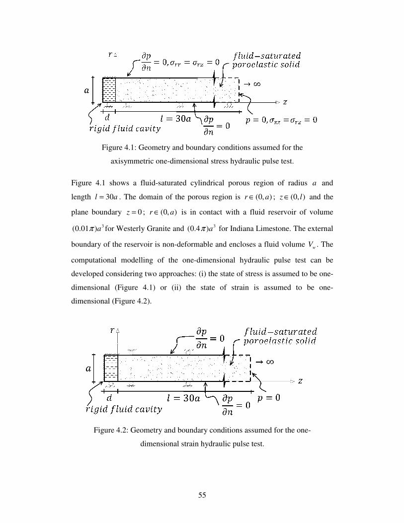
55

Figure 4.1: Geometry and boundary conditions assumed for the

axisymmetric one-dimensional stress hydraulic pulse test.

Figure 4.1 shows a fluid-saturated cylindrical porous region of radius a and

length 30l a= . The domain of the porous region is (0, )r a∈ ; (0, )z l∈ and the

plane boundary 0z = ; (0, )r a∈ is in contact with a fluid reservoir of volume

3(0.01 )aπ for Westerly Granite and 3(0.4 )aπ for Indiana Limestone. The external

boundary of the reservoir is non-deformable and encloses a fluid volume w

V . The

computational modelling of the one-dimensional hydraulic pulse test can be

developed considering two approaches: (i) the state of stress is assumed to be one-

dimensional (Figure 4.1) or (ii) the state of strain is assumed to be one-

dimensional (Figure 4.2).

Figure 4.2: Geometry and boundary conditions assumed for the one-

dimensional strain hydraulic pulse test.

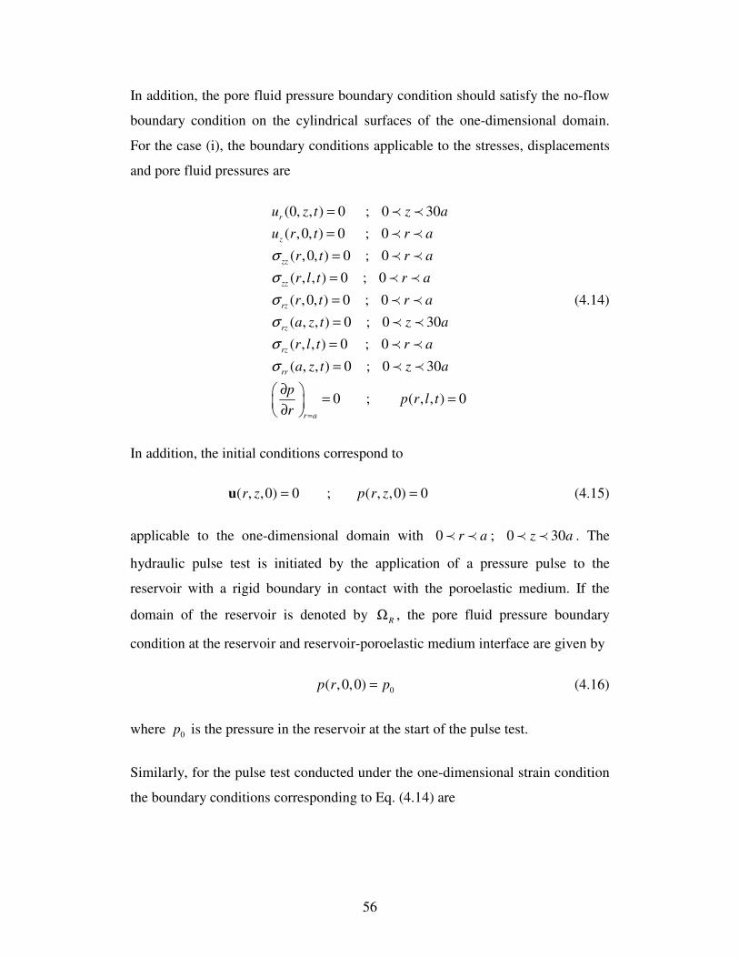
56

In addition, the pore fluid pressure boundary condition should satisfy the no-flow

boundary condition on the cylindrical surfaces of the one-dimensional domain.

For the case (i), the boundary conditions applicable to the stresses, displacements

and pore fluid pressures are

(0, , ) 0 ; 0 30

( ,0, ) 0 ; 0

( ,0, ) 0 ; 0

( , , ) 0 ; 0

( ,0, ) 0 ; 0

( , , ) 0 ; 0 30

( , , ) 0 ; 0

( , , ) 0 ; 0 30

0 ; ( , , ) 0

r

z

zz

zz

rz

rz

rz

rr

r a

u z t z a

u r t r a

r t r a

r l t r a

r t r a

a z t z a

r l t r a

a z t z a

pp r l t

r

σ

σ

σ

σ

σ

σ

=

=

=

=

=

=

=

=

=

∂ = =

∂

p p

p p

p p

p p

p p

p p

p p

p p

(4.14)

In addition, the initial conditions correspond to

( , ,0) 0 ; ( , ,0) 0r z p r z= =u (4.15)

applicable to the one-dimensional domain with 0 r ap p ; 0 30z ap p . The

hydraulic pulse test is initiated by the application of a pressure pulse to the

reservoir with a rigid boundary in contact with the poroelastic medium. If the

domain of the reservoir is denoted by R

Ω , the pore fluid pressure boundary

condition at the reservoir and reservoir-poroelastic medium interface are given by

0( ,0,0)p r p= (4.16)

where 0p is the pressure in the reservoir at the start of the pulse test.

Similarly, for the pulse test conducted under the one-dimensional strain condition

the boundary conditions corresponding to Eq. (4.14) are

57

( ,0, ) 0 ; (0, , ) 0

( , , ) 0 ; ( , , ) 0

( , , ) 0 ; ( ,0, ) 0

( , , ) 0

0 ; ( , , ) 0

rz r

rz r

rz z

zz

r a

r t u z t

a z t u a z t

r l t u r t

r l t

pp r l t

r

σ

σ

σ

σ

=

= =

= =

= =

=

∂ = =

∂

(4.17)

In Eq. (4.17) the extent of the region is specified by 0 r ap p and 0 30z ap p .

The initial conditions for the hydraulic pulse test conducted under one-

dimensional strain are identical to Eq. (4.15) and the pulse test is initiated by a

condition similar to Eq. (4.16).

Purely radial pulse testing was also examined (Figure 4.3). The modeled element

has a fluid cavity radius of a and a height of 20H a= for Westerly Granite and

0.5H a= for Indiana Limestone.

Unlike the one-dimensional model, here the size of the cavity can change as the

cavity pressure changes. The corresponding boundary conditions are:

0

2 2

(0, , ) 0 ; (0, , ) 0

( , , ) 0 ; ( , , ) 0

( , 2, ) 0 ; ( , 2, ) 0

(0, , ) 0

( , , ) 0 ; 0

0 ; 0

rr rz

rr rz

z z

r

r

z H z H

z t z t

R z t R z t

u r H t u r H t

u z t

pp R z t

r

p p

z z

σ σ

σ σ

=

=− =

= =

= =

− = =

=

∂ = =

∂

∂ ∂ = =

∂ ∂

(4.18)

In Eq. (4.18) the extent of the region is specified by 0 r Rp p and

2 2H z H− p p . The initial conditions for the purely radial flow pulse test are

again identical to Eq. (4.15) and the initiating pressure is

0( , ,0)p r z p= (4.19)

58

Figure 4.3: Schematic view for the radially symmetric hydraulic pulse

testing of an infinitely extended rock mass.

To further establish the accuracy of the fully coupled poroelastic modelling of the

hydraulic pulse test, the computational approach was applied to examine the one-

dimensional problem that is given by Hart and Wang (1998). The problem

involves a cylinder measuring 0.0254 m in radius and 0.0309 m in height. The

sample was sealed at the base and at the circumference such that no water flow

could take place through these surfaces. The upper surface ( (0, );r a z l∈ = ) was

subjected to a unit constant pore pressure pulse and the whole specimen was

under constant total stress for the duration of the experiment. Figure 4.4 shows the

geometry and boundary conditions of the problem.

Figure 4.4: The geometry and boundary conditions of the problem examined

by Hart and Wang (1998).

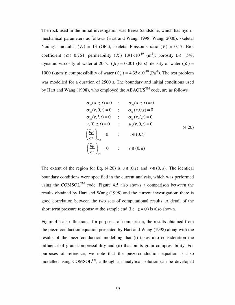
59

The rock used in the initial investigation was Berea Sandstone, which has hydro-

mechanical parameters as follows (Hart and Wang, 1998; Wang, 2000): skeletal

Young’s modulus ( E ) = 13 (GPa); skeletal Poisson’s ratio (ν ) = 0.17; Biot

coefficient (α )=0.764; permeability ( K% )=1.91×10-19 (m2); porosity (n) =5%;

dynamic viscosity of water at 20 ºC ( µ ) = 0.001 (Pa s); density of water ( ρ ) =

1000 (kg/m3); compressibility of water ( wC ) = 4.35×10-10 (Pa-1). The test problem

was modelled for a duration of 2500 s. The boundary and initial conditions used

by Hart and Wang (1998), who employed the ABAQUSTM code, are as follows

( , , ) 0 ; ( , , ) 0

( ,0, ) 0 ; ( ,0, ) 0

( , , ) 0 ; ( , , ) 0

(0, , ) 0 ; ( ,0, ) 0

0 ; (0, )

0 ; (0, )

rr rz

zz rz

zz rz

r z

r a

z l

a z t a z t

r t r t

r l t r l t

u z t u r t

pz l

r

pr a

r

σ σ

σ σ

σ σ

=

=

= =

= =

= =

= =

∂ = ∈

∂

∂ = ∈

∂

(4.20)

The extent of the region for Eq. (4.20) is (0, )z l∈ and (0, )r a∈ . The identical

boundary conditions were specified in the current analysis, which was performed

using the COMSOLTM code. Figure 4.5 also shows a comparison between the

results obtained by Hart and Wang (1998) and the current investigation; there is

good correlation between the two sets of computational results. A detail of the

short term pressure response at the sample end (i.e. 0z = ) is also shown.

Figure 4.5 also illustrates, for purposes of comparison, the results obtained from

the piezo-conduction equation presented by Hart and Wang (1998) along with the

results of the piezo-conduction modelling that (i) takes into consideration the

influence of grain compressibility and (ii) that omits grain compressibility. For

purposes of reference, we note that the piezo-conduction equation is also

modelled using COMSOLTM, although an analytical solution can be developed

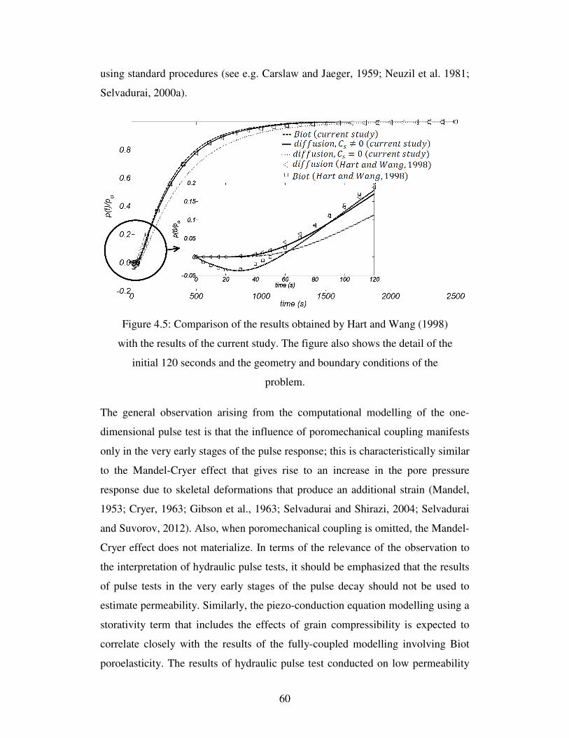
60

using standard procedures (see e.g. Carslaw and Jaeger, 1959; Neuzil et al. 1981;

Selvadurai, 2000a).

Figure 4.5: Comparison of the results obtained by Hart and Wang (1998)

with the results of the current study. The figure also shows the detail of the

initial 120 seconds and the geometry and boundary conditions of the

problem.

The general observation arising from the computational modelling of the one-

dimensional pulse test is that the influence of poromechanical coupling manifests

only in the very early stages of the pulse response; this is characteristically similar

to the Mandel-Cryer effect that gives rise to an increase in the pore pressure

response due to skeletal deformations that produce an additional strain (Mandel,

1953; Cryer, 1963; Gibson et al., 1963; Selvadurai and Shirazi, 2004; Selvadurai

and Suvorov, 2012). Also, when poromechanical coupling is omitted, the Mandel-

Cryer effect does not materialize. In terms of the relevance of the observation to

the interpretation of hydraulic pulse tests, it should be emphasized that the results

of pulse tests in the very early stages of the pulse decay should not be used to

estimate permeability. Similarly, the piezo-conduction equation modelling using a

storativity term that includes the effects of grain compressibility is expected to

correlate closely with the results of the fully-coupled modelling involving Biot

poroelasticity. The results of hydraulic pulse test conducted on low permeability

61

geomaterials can be expected to produce differing responses depending on (i) the

use of fully coupled analyses, (ii) the piezo-conduction equation that uses the

conventional definition of storativity, which includes compressibilities of the pore

fluid and the porous skeleton, (iii) the piezo-conduction equation that takes into

consideration the definition of storativity including fluid compressibility, skeletal

compressibility and grain compressibility, and (iv) the state of deformation and

flow associated with the hydraulic pulse test (i.e. axial flow, one-dimensional

tests, radial flow well tests, etc.).

In order to examine the relative influences of factors (i) to (iv) on the results of

pulse tests, computational simulations were carried out for hypothetical hydraulic

pulse tests conducted on typical rocks such as Westerly Granite and Indiana

Limestone. The input data used in the computational simulations is given in Table

4.1.

Table 4.1: The mechanical, physical and hydraulic parameters applicable to

Westerly Granite and Indiana Limestone

Rock Type E ν α K% n

(GPa) (m2) %

Westerly Granitea 37.5 0.25 0.47 4.0×10-19 1.0

Indiana Limestoneb 24 0.14 0.85 73.75×10-15 16.6

aWang (2000) bSelvadurai and Selvadurai (2010)

Table 4.2 gives the values for the compressibilities and storativity terms used in

the model. The computational results for the one-dimensional and radial flow

hydraulic pulse tests were conducted using the boundary conditions and initial

conditions defined by Eq. (4.14) to Eq. (4.20).

Figure 4.6 shows the mesh configuration used in the axial and radial flow

modelling. The interface between the fluid cavity and the rock was modelled

62

using a very fine mesh to account for the Heaviside step function-type

discontinuous pressure gradients that will be present at the start of the test, when

the pore fluid pressure in the saturated geomaterial is set to zero everywhere

within the region.

Table 4.2: Storativity terms* for Westerly Granite and Indiana Limestone

Rock type eff

C

(Pa-1)

sC

(Pa-1)

Sε

(Pa-1)

Sσ

(Pa-1)

CS

(Pa-1)

Westerly

Granite 4.00×10-11 2.12×10-11 1.43×10-11 2.31×10-11 4.45×10-11

Indiana

Limestone 9.00×10-11 1.35×10-11 8.46×10-11 1.50×10-10 1.65×10-10

*In all estimates for S, the compressibility of water is taken as 4.54×10-10

(Pa-1) (White, 1986)

Figure 4.6: Mesh configuration for modelling: (a) one-dimensional

hydraulic pulse test (25028 elements), (b) radially symmetric hydraulic

pulse test (30017 elements).

63

A Lagrange-quadratic element with three degrees of freedom at each node was

used in the finite element model. The displacements and pore fluid pressure are

prescribed at all nodes.

Figures 4.7 and 4.8 illustrate, respectively, the computational results for one-

dimensional and radial flow hydraulic pulse tests conducted on Westerly Granite

and Indiana Limestone.

Figure 4.7: Comparison of the pressure decay curves obtained from Biot’s

theory of poroelasticity with those obtained using the piezo-conduction

equation for the one-dimensional hydraulic pulse test.

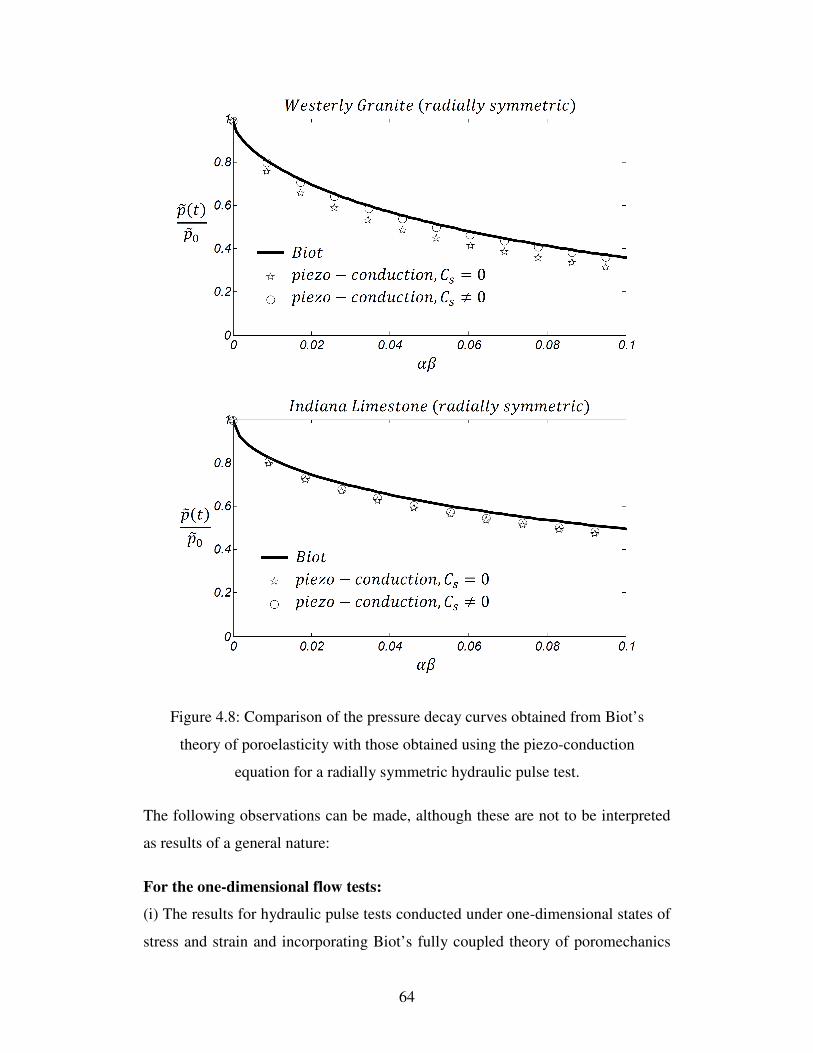
64

Figure 4.8: Comparison of the pressure decay curves obtained from Biot’s

theory of poroelasticity with those obtained using the piezo-conduction

equation for a radially symmetric hydraulic pulse test.

The following observations can be made, although these are not to be interpreted

as results of a general nature:

For the one-dimensional flow tests:

(i) The results for hydraulic pulse tests conducted under one-dimensional states of

stress and strain and incorporating Biot’s fully coupled theory of poromechanics

65

give very close results for one-dimensional Westerly Granite and relatively close

results for the Indiana Limestone (maximum discrepancy of 1.3 %).

(ii) The piezo-conduction equation analysis that also incorporates the influence of

grain compressibility provides a closer correlation with the results obtained from a

Biot poroelastic analysis with a one-dimensional stress condition. This is not an

unexpected result since the fully coupled Biot model takes into account the

influence of grain compressibility through the inclusion of the α parameter.

For the radial flow tests:

(i) In general, the radial flow hydraulic pulse tests are less influenced by fully

poroelastic coupling when compared to the one-dimensional axial flow hydraulic

pulse tests. The results for the fully coupled poroelastic hydraulic pulse decay

compare favorably with the piezo-conduction equation results that incorporate

grain compressibility.

(ii) The result from the conventional piezo-conduction equation analysis tends to

under-estimate the permeability of the medium.

There is no single non-dimensional parameter that would allow an identification

of the discrepancy that might be expected between the fully coupled analysis and

the conventional piezo-conduction equation analysis (with or without

consideration of grain compressibility). It would appear that the discrepancies

between the fully coupled analysis of the hydraulic pulse test and the result

derived from the conventional piezo-conduction equation with storativity defined

by Eq. (4.1) becomes more noticeable as the permeability of the material

decreases.

4.2.4. The effect of aspect ratio on the coupling behaviour

It is well known that under certain conditions the pressure diffusion equation (i.e.

Eq. (3.48)) decouples from the skeletal deformation (i.e. ( . ) 0t

α∂

∇ →∂

u ). Two of

these conditions are the irrotational displacement in the finite or semi-finite

66

domains (e.g. radially symmetric hydraulic pulse testing in an infinite medium)

and the limit of the relatively compressible pore fluid (Detournay and Cheng,

1993). It should, however, be noted that in such limiting cases the pore pressure

decay obtained from the piezo-conduction equation is not equal to that obtained

from Biot’s poroelasticity formulation, since the estimates for storativity are

different in the two formulations. The effect of the sample dimensions on the

coupling parameters in Biot’s poroelasticity has been studied by a number of

researchers (Detournay and Cheng, 1993; Lecampion et al., 2006). Since slender

samples were utilized in the previously cited computational treatments

( / 30L a ≈ ), the influence of the aspect ratio on the decay of the hydraulic pulse

was briefly investigated. The size of the cavity was kept constant for both one-

dimensional and radial flow hydraulic pulse tests and either the length or the outer

radius of the porous domain was changed. The hydraulic pulse tests were modeled

for different sample sizes using the linear equations of poroelasticity and also for

the piezo-conduction equation, with or without taking into account the

compressibility of the solid grains. The problem was modeled for each geometry

for the first 50% reduction in the cavity pressure obtained from the Biot

poroelasticity formulation and then re-examined using the piezo-conduction

equation over the same time duration. Finally, the cavity pressure at the end of

each modelling exercise was compared with the poroelasticity solution to obtain

the percentage error ( ( )(%) 100 /p c Biot Biotp p pδ −= × − ) in the estimation of

cavity pressure using the piezo-conduction equation. Figures 4.9 and 4.10 show

the calculated percentage error for, respectively, the one-dimensional and radially

symmetric hydraulic pulse tests. It is evident that for both the one-dimensional

and radially symmetric problems the piezo-conduction equation provides results

close to Biot’s poroelasticity solution and, for smaller aspect ratios, the

discrepancy between the results obtained from the two solutions becomes

negligible.

67

Figure 4.9: Comparison of the computational results obtained from the Biot

poroelasticity equations with the piezo-conduction equation for one-

dimensional constant stress and constant strain hydraulic pulse testing for

different aspect ratios.

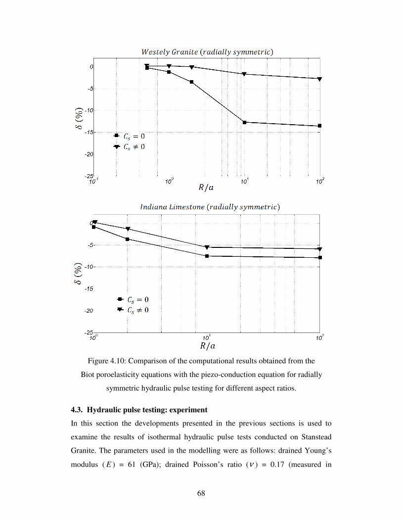
68

Figure 4.10: Comparison of the computational results obtained from the

Biot poroelasticity equations with the piezo-conduction equation for radially

symmetric hydraulic pulse testing for different aspect ratios.

4.3. Hydraulic pulse testing: experiment

In this section the developments presented in the previous sections is used to

examine the results of isothermal hydraulic pulse tests conducted on Stanstead

Granite. The parameters used in the modelling were as follows: drained Young’s

modulus ( E ) = 61 (GPa); drained Poisson’s ratio (ν ) = 0.17 (measured in

69

accordance with ASTM D7012-04); Biot coefficient (α )=0.44; porosity (n)

=0.5% to 1.4% (measured in accordance with ASTM D4404-84); dynamic

viscosity of water at 20 ºC ( µ ) = 0.001 (Pa.s) (White, 1986); density of water ( ρ )

= 1000 (kg/m3); compressibility of water ( wC ) = 4.54×10-10 (Pa-1) (White, 1986).

The value of the dynamic viscosity ( µ ) was adjusted to account for the actual

water temperature recorded for each test (White, 1986). Two types of hydraulic

pulse tests were conducted on the granite. The first involved pulse testing

cylindrical samples of the granite under purely radial flow conditions and the

second used an axisymmetric patch pulse test.

4.3.1. Radially symmetric hydraulic pulse tests

The cylindrical sample used in the experimental investigations measured 15.24

cm in diameter and 14.76 cm in height. The cylindrical surfaces of the samples

were cored from a larger sample and the plane ends were machined smooth to

accommodate a sealing gasket. The central cavity was prepared using a 2.54 cm

diameter diamond drill and the surface of the cavity was air-blown to remove any

debris that might be embedded on the surface of the cavity that could impede fluid

flow by clogging the pore space.

Radial flow hydraulic pulse testing involves the application of a pressure pulse to

a central cavity drilled into the rock specimen. The sample was vacuum saturated

for a period of 7 days to ensure that the pore space was saturated. There are no

assurances that the entire pore space would be saturated but experience from

previous experimental investigations involving cement grouts (Selvadurai and

Carnaffan, 1997), Barre Granite (Selvadurai et al., 2005), Indiana Limestone

(Selvadurai, 2009) and Cobourg Limestone (Selvadurai and Jenner, 2013) using

such techniques have resulted in reliable results concerning saturation. The plane

surfaces of the hollow cylinder were sealed with BondoTM fibreglass resin to

ensure that the flow pattern corresponds to radial flow (see e.g. Jenner, 2012). A

schematic view of the experimental faculty is shown in Figure 4.11.

70

Figure 4.11: Experimental faculty for measuring the permeability of low

permeability geomaterials (Frame designed by Mr. A. Chevrier, Carlton

University).

The apparatus consists of a test frame to provide a seal between the centrally

cored Stanstead Granite specimen and a stainless steel “permeameter” that has a

water inflow, an outlet and a connection to a 1400 kPa Honeywell pressure

transducer. This arrangement, in principle, is the same as experimental technique

used by Carnaffan (1994) and Selvadurai and Carnaffan (1997) when performing

hydraulic pulse tests on cementitious grout and by Selvadurai and Selvadurai

(2010) when performing steady state patch permeability tests. The permeameter

has provisions for extracting air from the central cavity that could influence the

performance of the hydraulic pulse test. Figure 4.12 shows the details of the

permeameter.

The procedure for performing the radial flow pulse test involves a preliminary test

that is performed on a machined aluminum cylinder to test the efficiency of the

seals used to maintain radial flow. In these trial tests, the upper flat surface of the

aluminum cylinder was covered with epoxy in exactly the same way as the

71

surface of the granite sample. A sealing pressure of 1.5 MPa was applied to the O-

ring contact area and three hydraulic pulse tests were performed. The load applied

to the sample for sealing purposes was measured using a 45 kN Futek load cell.

Each test started with the instantaneous build up of pressure in the permeameter

cavity.

Figure 4.12: Components of the permeameter used to perform hydraulic

pulse tests on fully-drilled samples.

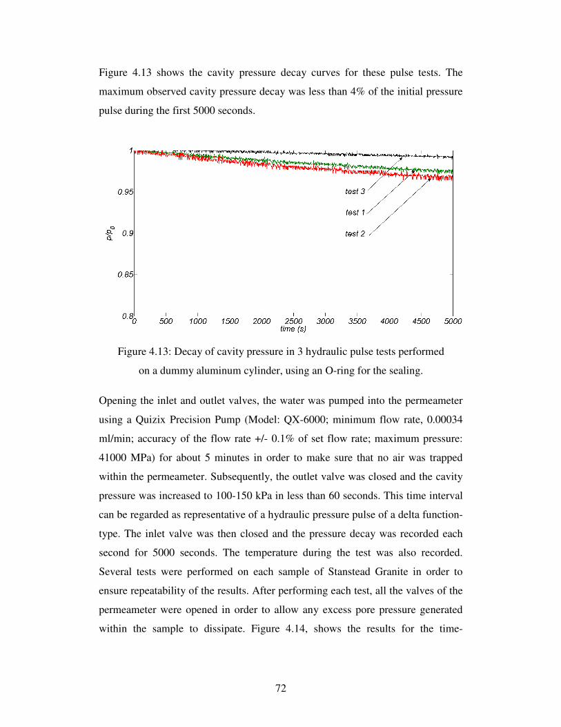
72

Figure 4.13 shows the cavity pressure decay curves for these pulse tests. The

maximum observed cavity pressure decay was less than 4% of the initial pressure

pulse during the first 5000 seconds.

Figure 4.13: Decay of cavity pressure in 3 hydraulic pulse tests performed

on a dummy aluminum cylinder, using an O-ring for the sealing.

Opening the inlet and outlet valves, the water was pumped into the permeameter

using a Quizix Precision Pump (Model: QX-6000; minimum flow rate, 0.00034

ml/min; accuracy of the flow rate +/- 0.1% of set flow rate; maximum pressure:

41000 MPa) for about 5 minutes in order to make sure that no air was trapped

within the permeameter. Subsequently, the outlet valve was closed and the cavity

pressure was increased to 100-150 kPa in less than 60 seconds. This time interval

can be regarded as representative of a hydraulic pressure pulse of a delta function-

type. The inlet valve was then closed and the pressure decay was recorded each

second for 5000 seconds. The temperature during the test was also recorded.

Several tests were performed on each sample of Stanstead Granite in order to

ensure repeatability of the results. After performing each test, all the valves of the

permeameter were opened in order to allow any excess pore pressure generated

within the sample to dissipate. Figure 4.14, shows the results for the time-

73

dependent pressure decay obtained during 10 pulse tests conducted on Stanstead

Granite.

The interpretation of pulse tests to estimate the permeability can be performed in a

variety of ways and the most convenient procedure is to develop a set of pulse

decay curves that can be used to “bound” the value of permeability (Selvadurai

and Carnaffan, 1997; Selvadurai et al., 2005). The bounding procedure for

obtaining a range of values for K% is considered to be more realistic than obtaining

a specific value. The bounding data were determined from three different

approaches: (i) the conventional piezo-conduction equation analyses ( pcK% ), (ii)

the conventional piezo-conduction equation, which also accounts for the

compressibility of grains, analyses ( pccK% ), and (iii) a fully coupled analysis of the

radial flow pulse decay problem ( fcK% ).

Figure 4.14: Results of hydraulic pulse tests performed on a fully drilled

Stanstead Granite cylinder (sample SD). The analysis of the data was done

using the piezo-conduction equation and neglecting the compressibility of

the solid grains.

The bounding curves shown in Figure 4.14 are only estimates based on the

approach (i) while Table 4.3 summarizes the permeability ranges estimated from

74

all three methods. There are only marginal differences between the three

estimates.

Table 4.3: Permeability values for Stanstead Granite.

Sample fcK% (m2) pccK% (m

2) pcK% (m2)

SU (1.2 to 1.7)×10-20 (1.2 to 1.7)×10-20 (1.1 to 1.6)×10-20

SD (6.0 to 7.7)×10-20 (6.0 to 7.7)×10-20 (5.5 to 7.0)×10-20

4.3.2. Patch pulse tests

We next consider the problem of pulse loading applied at a patch located on the

plane surface of a cylinder of Stanstead Granite. The patch pulse tests have been

successfully used to estimate the permeability characteristics of rocks such as

Berea Sandstone (Tidwell and Wilson, 1997) and Indiana Limestone (Selvadurai

and Selvadurai, 2010). Here we present an application that investigates the

transient behaviour of a hydraulic pulse applied at a circular opening located at

the axis of the sealed plane surface of a cylindrical sample of Stanstead Granite.

The sealing between the permeameter and the granite cylinder is achieved by

applying an axial stress of 1.5 MPa. Similar to the O-ring sealing test, a series of

hydraulic pulse tests were performed on a Plexiglas plate to establish any leakage

from the sealing technique. The permeameter was placed on top of a Plexiglas

surface and a sealing stress of 1.5 MPa was applied to the gasket.

Figure 4.15 shows the results of 5 hydraulic pulse tests. A maximum cavity

pressure drop of 8% was observed during the first 5000 seconds. The pressure

pulses applied within the opening are kept to a maximum of 150 kPa to eliminate

any leakage at the sample-rubber gasket interface. The procedure adopted to

constrain the gasket during its compression is similar to that used by Selvadurai

(2010) and Selvadurai and Selvadurai (2010) and provides a successful sealing

technique. A schematic view of the test arrangement is shown in Figure 4.16.

75

Figure 4.15: Decay of cavity pressure in hydraulic pulse tests performed on

a Plexiglas, using gasket for the sealing.

Figure 4.16: Components of the permeameter used to perform hydraulic

pulse tests on undrilled samples.

76

The gasket has an inner diameter of 2.54 cm and an outer diameter of 10.16 cm.

The annular region of the plane surface of the cylinder is maintained in a sealed

and submerged condition.

The residual pore pressure fields created during saturation of the sample under

vacuum were allowed to dissipate over a 7 day period. The fluid cavity was

subjected to a pressure pulse to initiate the pulse tests. Figure 4.17 shows the

results of surface pulse tests derived from 10 experiments conducted on the

cylindrical sample of Stanstead Granite.

Figure 4.17: Results of hydraulic pulse tests performed on an undrilled

Stanstead Granite cylinder (sample SU). The analysis of data was done using

the piezo-conduction equation and neglecting the compressibility of the

solid grains.

These results have been interpreted on the basis of the three sets of permeability

estimates explained for radial flow hydraulic pulse tests in previous section. These

estimated permeability values are also shown in Table 4.3. The pore pressure

boundary condition applicable to the patch pulse testing that uses the piezo-

conduction equation analysis (with and without the influence of grain

compressibility) are shown in Figure 4.18 (a) and the pore pressure, displacement

and traction boundary condition needed to perform a fully coupled analysis are

77

shown in Figure 4.18 (b). The results derived from the three sets of theoretical

estimates for the permeability predicted the correct trends for the pulse decay,

although the numerical predictions show deviations from the experimental data.

Figure 4.18: Sample SU: (a) Geometry and boundary conditions used for the

piezo-conduction equation; (b) Geometry and boundary conditions used for

Biot’s poroelasticity equations.

The likely causes for the discrepancies seen between the experimental

observations and theoretical predictions for the patch pulse tests could be due to

several factors including leakage, damage during sample fabrication, transverse

isotropy influences of permeability and air entrapment. The first two factors can

be eliminated since this would have resulted in faster decay rates than those

presented in Figure 4.17. There is little information on the estimation of

permeability anisotropy of the Stanstead Granite. Literature on fracture toughness

testing suggests the presence of some anisotropy in the fracture toughness

properties (Nasseri et al., 2010). As a parametric exercise, hydraulic pulse test

78

behaviour was modelled with hydraulic transverse isotropy maintaining the range

of values of the radial hydraulic conductivity estimated from the purely radial

flow tests. It is estimated that the permeability in the axial direction should be 20

times smaller than the permeability in the radial direction in order to achieve a

correlation between the computational predictions provided by the fully coupled

analysis and the experimental data. Air entrapment in the system can be another

reason for the discrepancy, the effect of which will be further discussed in

Chapter 5.

4.4. Summary

In this chapter, the use of the hydraulic pulse technique for measuring the

permeability of low permeability geomaterials was discussed. The range of

applicability of the piezo-conduction equation used to estimate the hydraulic

properties of low permeability rocks was examined using Biot’s poroelasticity

theory. The results indicate that the prediction for the pressure decay can be

influenced by both the model used to interpret the test and the test configuration;

this in turn can influence the interpretation of the permeability of the porous

medium. Conventional modelling of the test that uses the piezo-conduction

equation does not account for the compressibility of the solid grains and this

factor can have an influence on the estimation of the permeability of geomaterials

with small Biot coefficient. A further consideration is the influence of generalized

deformations of the porous skeleton; this can be accommodated for by modelling

the piezo-conduction equation by appeal to Biot’s classical theory of

poroelasticity. The incorporation of the generalized deformations can also

influence the interpretation of test results. The performance of the two modelling

techniques is demonstrated by examining the pulse decay observed in two typical

geologic media that have been investigated in the literature. Finally, the results of

hydraulic pulse tests performed on two Stanstead Granite samples were analyzed

by employing the separate approaches. Comparisons show that, although the

permeability obtained from the different approaches change, the order of

magnitude is consistent for the performed tests. Also, the computational studies

performed show that the choice of a modelling technique has a greater influence

79

on the one-dimensional hydraulic pulse test than the radially symmetric test

configurations. In general, the most complete approach to analyze the hydraulic

pulse test results is to use Biot’s poroelasticity theory, which accounts for

deformability of the solid grains and models the coupled interaction of the porous

skeleton deformation and the pressure change. This technique, however, is

complicated and time consuming to employ. For simplicity, the permeability

parameter can be estimated using the piezo-conduction equation that accounts for

grain compressibility.

80

CHAPTER 5

THE EFFECT OF AIR ON THE INTERPRETATION OF HYDRAULIC PULSE TESTS

5.1. Introduction

The hydraulic pulse testing technique incorporates the compressibility of the

constituents of the fluid-saturated porous medium, which includes the skeleton,

the solid grains and the pore fluid. Each hydraulic pulse test starts with rapid

pressurization of the fluid cavity in contact with a surface of the sample. The inlet

valve to the cavity is then closed and the fluid cavity pressure dissipation is

monitored. Since the compressibility of the pressurized fluid is low, a minimal

migration of fluid to the porous medium causes the pressure in the cavity to drop.

The compressibility of pure water at 20 o C is 4.54×10-10 Pa-1 (White, 1986),

which is defined as the relative volume decrease induced by the pressure increase.

As an example, a 100 kPa pressure drop in an arbitrary 20 ml fluid-filled cavity

corresponds to 9.0×10-4 ml of fluid loss. Therefore, the technique provides the

resolution required to measure very small amounts of fluid flow, which makes the

transient measurement of permeability of tight rocks feasible. However, the

entrapment of air bubbles in the fluid cavity can significantly affect the

compressibility of water. It was noted by Fredlund (1976) that air inclusion of

only 1% increases the compressibility of water by three orders of magnitude.

81

Since, in practice, it is almost impossible to avoid air entrapment in the sealed

fluid cavity used in hydraulic pulse testing, the effect of this phenomenon should

be taken into account. The effects of compressibility of the air-water mixture was

also studied by Schuurman (1966), Fredlund (1976), Teunissen (1982),

Pietruszczak and Pande (1996), and Selvadurai and Ichikawa (2013).

5.2. Governing equations

Air can exist in water in two different forms: dissolved air and air in a gaseous

form. Assuming that the air inclusions in the water is in the form of bubbles and

neglecting the effects of the solubility of air in the water, the surface tension of

the water and the vapour pressure, the compressibility of the air-water mixture can

be calculated. The total volume of the mixture ( tV ) is composed of pure water

( wV ) and air bubbles ( aV ). The air fraction is defined as

a

w a

V

V Vϕ =

+ (5.1)

The isothermal compressibility of the mixture, pure water, and the air inclusion

are, respectively, defined as

; ;

t w a

t w aeq w a

dV dV dV

V V VC C C

dp dp dp= − = − = − (5.2)

Substituting t w a

V V V= + in the compressibility equation of the mixture (i.e. Eq.

(5.2)) gives

( ) ( )t w a

t w a w aeq

dV dV dV

V V V V VC

dp dp dp

+ += − = − − (5.3)

The two terms in the right hand side of Eq. (5.3) can be re-written in the form of

aC and

wC

82

1 1 1; (1 ) (1 )a a w w

a w

a w a a w

dV dV dV dVC C

V V dp V dp V V dp dpϕ ϕ ϕ ϕ= = = − = −

+ + (5.4)

Substituting Eq. (5.4) into Eq. (5.3) gives

(1 )eq a w

C C Cϕ ϕ= + − (5.5)

Eq. (5.5) gives the compressibility of a fluid-gas mixture with free air bubbles.

The compressibility of air can be derived by considering the incremental

variations to Boyle’s Law in an isothermal condition; i.e.

1. ; 0

a

aa a a a

dV

VPV const PdV V dP C

dP P

−

= + = ⇒ = = (5.6)

where P is the absolute air pressure.

Boyle’s law also determines the changes of air fraction with pressure. Assuming

that the total volume of cavity (i.e. w a

V V+ ) is constant during hydraulic pressure

decay , the air fraction equation can be re-written as

00

00 0 0;

aa

a a

w a w a

PV

V PPP V PVV V V V P

ϕ ϕ ϕ= = ⇒ = =+ +

(5.7)

where 0P is the initial absolute water pressure, 0a

V is the initial volume of air, and

0ϕ is the initial air fraction in the cavity.

Figure 5.1 shows the effect of the air fraction in the form of air bubbles on the

compressibility of the air-water mixture (the effect of solubility of air is neglected,

i.e. h=0).

83

Figure 5.1: Compressibility of air-water mixtures with different air

fractions.

From Figure 5.1 it can be seen that the amount of air inclusion has a significant

effect on the compressibility of the mixture. For instance, for an air fraction of

1%, the compressibility is in the range of 1×10-9 (Pa-1) to 1×10-7 (Pa-1). Therefore,

compared to the compressibility of de-aired water, only a 1% air fraction can

increase the compressibility of the mixture by three orders of magnitude, (as also

noted by Fredlund (1976).

Air can dissolve in water without any chemical interaction and occupy a certain

volume of the water. This volume is only temperature-dependent; Henry’s Law

states that the weight of gas dissolved in a certain quantity of liquid at a constant

temperature is directly proportional to the pressure of the gas above the solution.

Also, Fick’s Law can be used to describe the rate at which air goes into solution.

Based on Henry’s Law, the maximum volume fraction of air in solution is

(1 )h ϕ− , where h is Henry’s constant and ϕ is the air fraction. Thus, in order to

take into account the effect of gas solubility on the compressibility of the gas-fluid

mixture, Eq. (5.6) is modified as follows

(1 )(1 )

eq w

hC C

P

ϕ ϕϕ

+ −= + − (5.8)

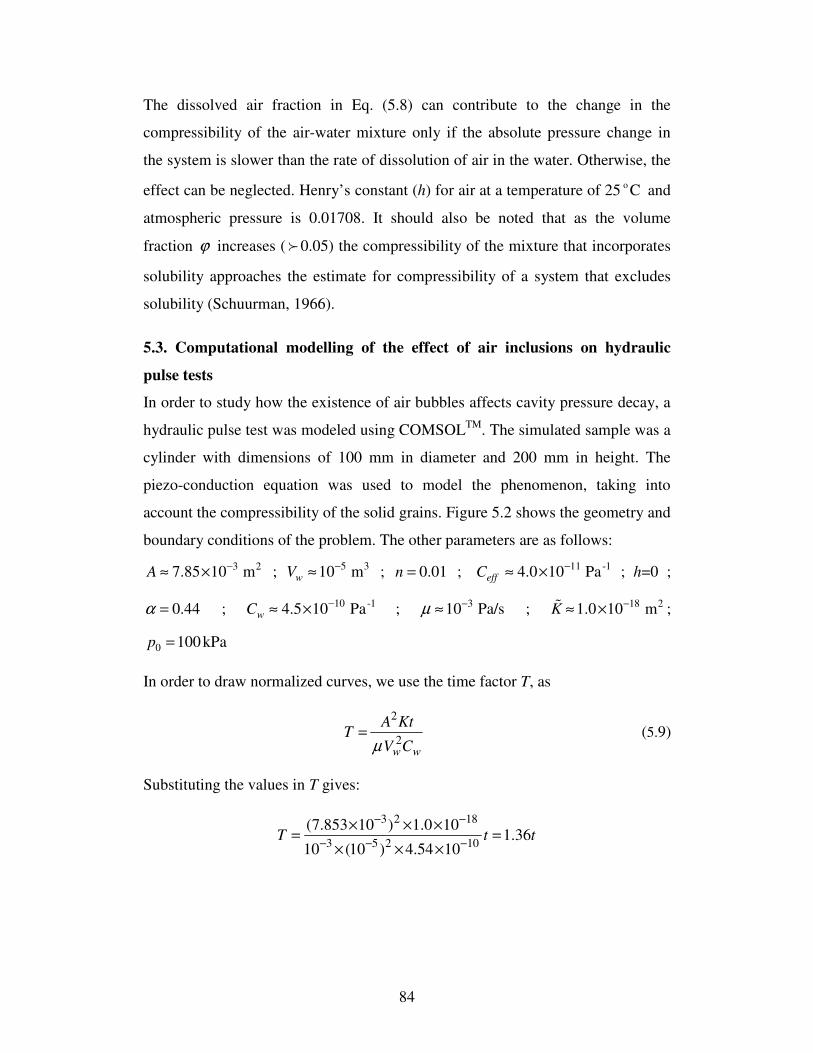
84

The dissolved air fraction in Eq. (5.8) can contribute to the change in the

compressibility of the air-water mixture only if the absolute pressure change in

the system is slower than the rate of dissolution of air in the water. Otherwise, the

effect can be neglected. Henry’s constant (h) for air at a temperature of 25 o C and

atmospheric pressure is 0.01708. It should also be noted that as the volume

fraction ϕ increases (f 0.05) the compressibility of the mixture that incorporates

solubility approaches the estimate for compressibility of a system that excludes

solubility (Schuurman, 1966).

5.3. Computational modelling of the effect of air inclusions on hydraulic

pulse tests

In order to study how the existence of air bubbles affects cavity pressure decay, a

hydraulic pulse test was modeled using COMSOLTM. The simulated sample was a

cylinder with dimensions of 100 mm in diameter and 200 mm in height. The

piezo-conduction equation was used to model the phenomenon, taking into

account the compressibility of the solid grains. Figure 5.2 shows the geometry and

boundary conditions of the problem. The other parameters are as follows:

3 27.85 10 mA −≈ × ; 5 310 mwV−≈ ; 0.01n = ; 11 -14.0 10 PaeffC

−≈ × ; h=0 ;

0.44α = ; 10 -14.5 10 PawC−≈ × ; 310 Pa/sµ −≈ ; 18 21.0 10 mK −≈ ×% ;

0 100kPap =

In order to draw normalized curves, we use the time factor T, as

2

2w w

A KtT

V Cµ= (5.9)

Substituting the values in T gives:

3 2 18

3 5 2 10

(7.853 10 ) 1.0 101.36

10 (10 ) 4.54 10T t t

− −

− − −

× × ×= =

× × ×

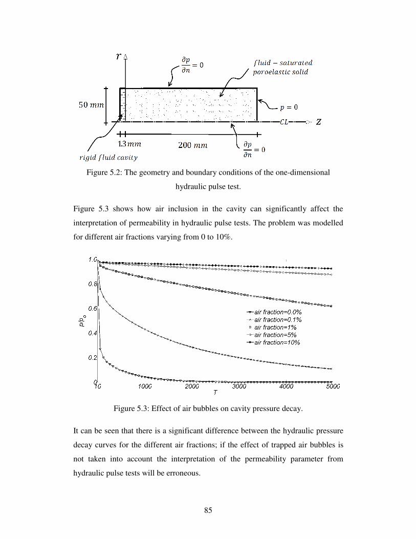
85

Figure 5.2: The geometry and boundary conditions of the one-dimensional


Figure 5.3 shows how air inclusion in the cavity can significantly affect the

interpretation of permeability in hydraulic pulse tests. The problem was modelled

for different air fractions varying from 0 to 10%.

Figure 5.3: Effect of air bubbles on cavity pressure decay.

It can be seen that there is a significant difference between the hydraulic pressure

decay curves for the different air fractions; if the effect of trapped air bubbles is

not taken into account the interpretation of the permeability parameter from

hydraulic pulse tests will be erroneous.

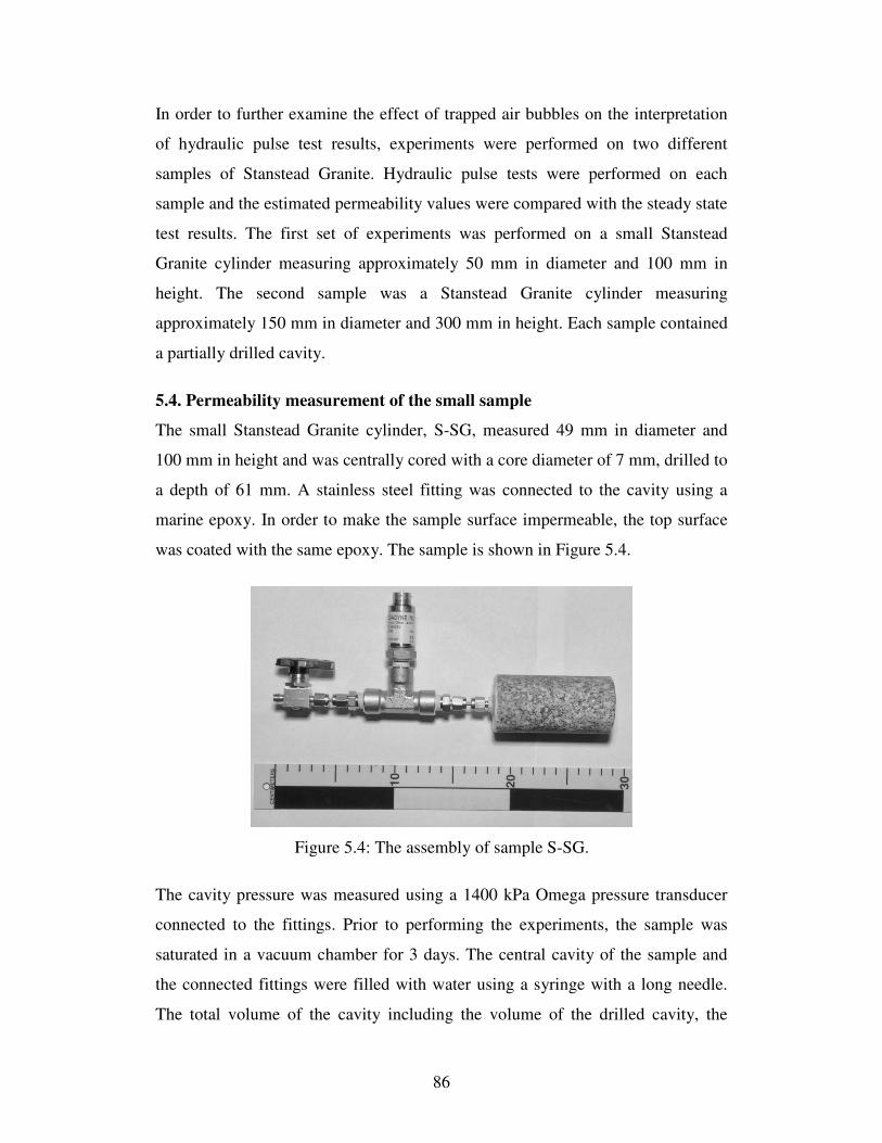
86

In order to further examine the effect of trapped air bubbles on the interpretation

of hydraulic pulse test results, experiments were performed on two different

samples of Stanstead Granite. Hydraulic pulse tests were performed on each

sample and the estimated permeability values were compared with the steady state

test results. The first set of experiments was performed on a small Stanstead

Granite cylinder measuring approximately 50 mm in diameter and 100 mm in

height. The second sample was a Stanstead Granite cylinder measuring

approximately 150 mm in diameter and 300 mm in height. Each sample contained

a partially drilled cavity.

5.4. Permeability measurement of the small sample

The small Stanstead Granite cylinder, S-SG, measured 49 mm in diameter and

100 mm in height and was centrally cored with a core diameter of 7 mm, drilled to

a depth of 61 mm. A stainless steel fitting was connected to the cavity using a

marine epoxy. In order to make the sample surface impermeable, the top surface

was coated with the same epoxy. The sample is shown in Figure 5.4.

Figure 5.4: The assembly of sample S-SG.

The cavity pressure was measured using a 1400 kPa Omega pressure transducer

connected to the fittings. Prior to performing the experiments, the sample was

saturated in a vacuum chamber for 3 days. The central cavity of the sample and

the connected fittings were filled with water using a syringe with a long needle.

The total volume of the cavity including the volume of the drilled cavity, the

87

fittings and the pressure transducer, was measured as 10 ml. Figure 5.5 shows the

schematic view of the experimental setup.

Figure 5.5: Schematic view of the hydraulic pulse test experiment

performed on sample S-SG.

5.4.1. Steady state tests

Initially, the permeability of the sample was measured using a steady state

technique under different flow rates of 0.0025, 0.005, 0.01, 0.02 ml/min. Figure

5.6 shows the cavity pressure recorded for the different flow rates. The problem

was modelled using COMSOL MultiphysicsTM. Table 5.1 shows the measured

steady state pressure corresponding to each flow rate and the estimated

permeability value.

The measured permeability was (3.45 to 3.55) ×10-18(m2). The cavity pressure

ranged from 55 kPa to 430 kPa and no pressure dependency was observed in the

permeability measurement using the steady state technique.

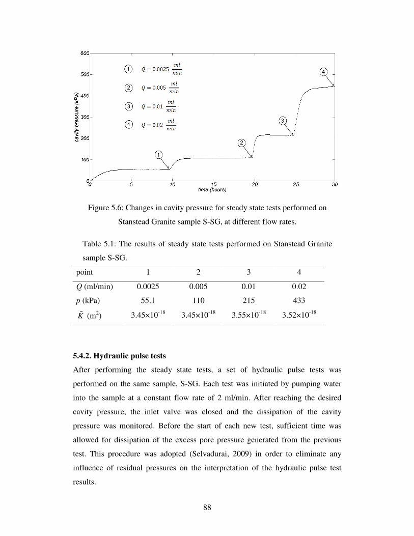
88

Figure 5.6: Changes in cavity pressure for steady state tests performed on

Stanstead Granite sample S-SG, at different flow rates.

Table 5.1: The results of steady state tests performed on Stanstead Granite

sample S-SG.

point 1 2 3 4

Q (ml/min) 0.0025 0.005 0.01 0.02

p (kPa) 55.1 110 215 433

K% (m2) 3.45×10-18 3.45×10-18 3.55×10-18 3.52×10-18

5.4.2. Hydraulic pulse tests

After performing the steady state tests, a set of hydraulic pulse tests was

performed on the same sample, S-SG. Each test was initiated by pumping water

into the sample at a constant flow rate of 2 ml/min. After reaching the desired

cavity pressure, the inlet valve was closed and the dissipation of the cavity

pressure was monitored. Before the start of each new test, sufficient time was

allowed for dissipation of the excess pore pressure generated from the previous

test. This procedure was adopted (Selvadurai, 2009) in order to eliminate any

influence of residual pressures on the interpretation of the hydraulic pulse test

results.

89

A total of 9 hydraulic pulse tests were performed on the sample. The target

maximum cavity pressure values were 100, 250, and 600 kPa. Three hydraulic

pulse tests were performed at each target pressure. The measured cavity pressure

changes were then analyzed using the COMSOL MultiphysicsTM software. The

piezo-conduction equation was used to model the phenomenon, taking into

account the compressibility of the solid grains. The parameters used in the

analysis were as follows: Young’s modulus (E) = 61 GPa, Poisson’s ratio (ν) =

0.17; porosity (n) = 0.5% to 1.4%; Biot coefficient (α ) = 0.44; compressibility of

the fluid (Cw) = 4.54×10-10 Pa-1. The measured cavity pressure curves along with

the computed bounding decay curves are shown in Figure 5.7. Compared to the

steady state tests, the hydraulic pulse test results showed very low permeability

values. The estimated permeability range is one to three orders of magnitude

different from the permeability value measured using the steady state technique.

Also, a clear pressure dependency was observed in the measured cavity pressure

dissipation curves. Since no pressure dependency was observed in the steady state

technique, referring to the Eq. (5.8) it can be concluded that it was associated with

the existence of air bubbles in the cavity.

Figure 5.7: Hydraulic pulse tests performed on sample Stanstead Granite S-

SG.

90

In order to take into account the effect that the compressibility of the air-water

mixture has on the analysis of the hydraulic pulse tests and estimate the amount of

trapped air in the fluid cavity, it was decided to study the pressure build-up

curves.

5.4.3. Back-calculation of compressibility change using the experimental

results

Assuming that the compressibility of the air-water mixture is eqC and that water is

pumped into the cavity at a constant flow rate, then

1t t

teq eq

t

dV dVV dtC C

dpdp Vdt

= − ⇒ = − (5.10)

where tV is the volume of cavity while it is being pressurized. The volume

includes the rock cavity, the cavity of the connection fittings and the volume of

the pump cylinder. From the definition

tdVQ

dt= − ; 0( )

t tV t V Qt= − (5.11)

where 0tV is the initial total volume of the cavity, we obtain

0eq

t

dp QC

dt V Qt=

− (5.12)

The above equation can be approximated by

( )0t

eq

Q V QtC

p t

−≈

∆ ∆ (5.13)

In order to estimate the variation in the compressibility of the cavity fluid, eqC

for the hydraulic pulse tests performed on the Stanstead Granite sample S-SG, the

pressure build-up curves recorded for the tests were used along with Eq. (5.13).

91

Figure 5.8 shows the change of eqC with pressure for the cavity pressure build-up

stage of the test. The range of compressibility of the cavity fluid was (7.0×10-9 to

3.4×10-7) Pa-1 for the applied pressure range, which is much higher than usually

assumed for the parameter. Therefore, the assumption of constant compressibility

of de-aired water, wC =4.54×10-10 (Pa-1), is not valid, since it introduces a

significant error in the interpretation of hydraulic pulse test results.

Figure 5.8: Change of eqC with cavity pressure increase in Stanstead Granite

sample S-SG.

Figure 5.9 shows the measured pressure build-up curve. In order to estimate the

air fraction trapped in the cavity, the build-up of pressure in the sample was

modelled using COMSOL MultiphysicsTM. The parameters used in the model are:

V0 = 30.1 ml (this includes the volumes of the rock cavity, the fittings, the

connection tube, and the volume of water in the pump cylinder), Q = 2 ml/min, K%

= (3.2×10-18 to 1.0×10-20) m2 and n = 0.5% to 1.4%. The pressure build-up curves

were fitted with the initial air fraction of 0ϕ =0.0298. Since the duration of

pressure build-up is short, variations in permeability of the rock within the range

of (3.2×10-18 to 1.0×10-20) m2 did not affect the pressure build-up curve.

92

Figure 5.9: Experimental results for the build-up of cavity pressure due to

pumping water at the rate of Q =2ml/min, for Stanstead Granite sample S-

SG.

5.4.4. Estimation of the permeability range

As shown in Figure 5.7, the hydraulic decay curves for the pulse tests are

dependent to the initial pressure, which cannot be explained by a constant eqC . In

order to estimate the permeability value, the results of hydraulic pulse tests were

analysed using the compressibility of the air-water mixture for the cavity fluid. It

was assumed that the sample was saturated and hence the compressibility of de-

aired water was used for modelling the specific storage of the porous medium.

The results were studied for the first 50% drop in the cavity pressure.

The air fraction estimated from the pressure build-up curves was obtained with

the assumption that the inlet valve was open, whereas during pressure decay the

inlet valve is closed. Hence, in order for the estimated air fraction to be used in

the analysis of hydraulic decay curves, it should be modified to account for the

reduced volume of cavity. In the current experiment, the initial air fraction was

estimated for a total fluid volume of 30.1 ml, whereas after closing the inlet valve

the volume of cavity that is connected to the porous medium occupies 10 ml.

Therefore, with the assumption that the air bubbles are trapped in the fittings

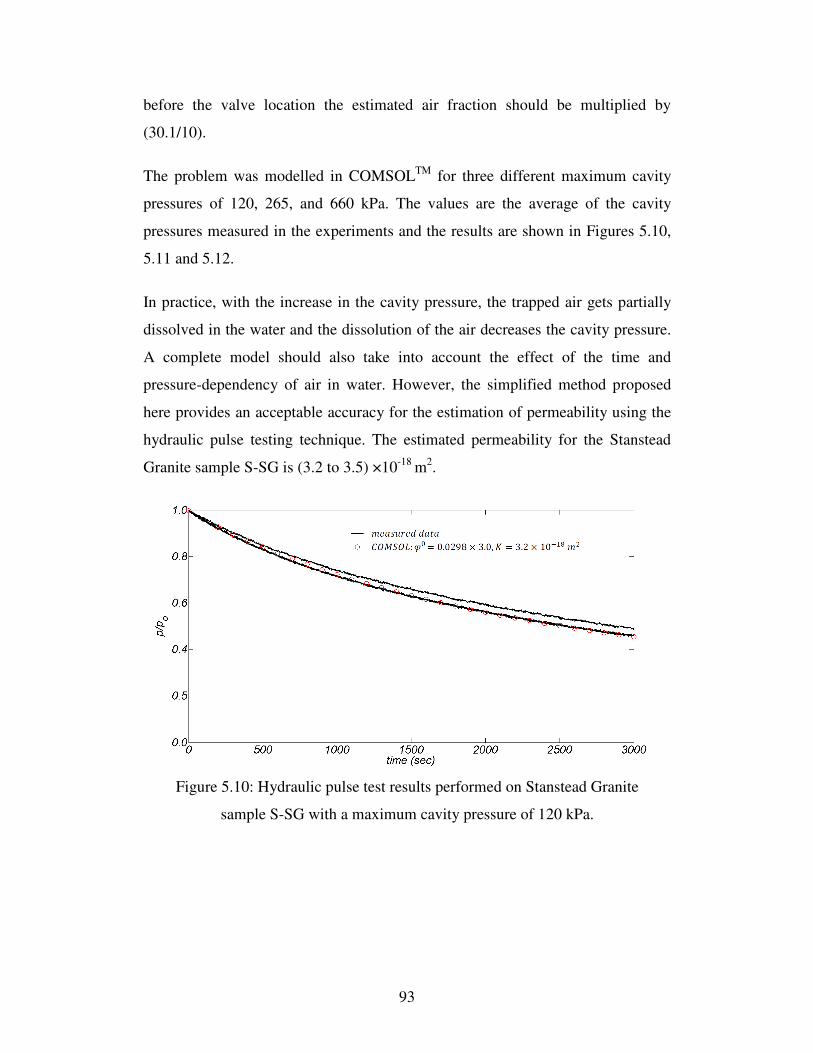
93

before the valve location the estimated air fraction should be multiplied by

(30.1/10).

The problem was modelled in COMSOLTM for three different maximum cavity

pressures of 120, 265, and 660 kPa. The values are the average of the cavity

pressures measured in the experiments and the results are shown in Figures 5.10,

5.11 and 5.12.

In practice, with the increase in the cavity pressure, the trapped air gets partially

dissolved in the water and the dissolution of the air decreases the cavity pressure.

A complete model should also take into account the effect of the time and

pressure-dependency of air in water. However, the simplified method proposed

here provides an acceptable accuracy for the estimation of permeability using the

hydraulic pulse testing technique. The estimated permeability for the Stanstead

Granite sample S-SG is (3.2 to 3.5) ×10-18 m2.

Figure 5.10: Hydraulic pulse test results performed on Stanstead Granite

sample S-SG with a maximum cavity pressure of 120 kPa.

94





5.4.5. Injecting air in the cavity

In order to further investigate the effect of air inclusion on the hydraulic pressure

decay, measured volumes of air were introduced to the fluid-filled cavity of

sample S-SG in two steps. The sample was initially immersed in water and the

fitting was connected to a Venturi pump that applied suction to the fluid-filled

cavity. A transparent plastic pipe was used to connect the vacuum pump to the

95

cavity fitting in order to observe the extracted air bubbles. The applied suction

helped to remove the trapped air bubbles from the cavity. The extraction of air

bubbles appeared to have stopped after almost a day of suction; however, the

suction was continued for another 24 hours in order to verify that the air bubble

extraction was complete. The vacuum pump was then turned off and the negative

pore pressure in the rock was allowed to dissipate for a day before starting the

hydraulic pulse tests. The experiments were conducted in three steps: (i) three

hydraulic pulse tests were performed on sample S-SG after suction removal of the

trapped air bubbles, (ii) three hydraulic pulse tests were performed after

deliberately introducing 0.035 ml of air into the fluid-filled cavity, and (iii) three

hydraulic pulse tests were conducted after introducing another 0.106 ml of air into

the fluid-filled cavity.

All of the hydraulic pulse tests commenced by pumping water into the cavity at a

constant flow rate of 2 ml/min. When the fluid pressure in the cavity reached 300

kPa, the inlet valve was closed. A syringe with a long needle was used to remove

water from the cavity for steps (ii) and (iii). The syringe was weighed before and

after removing water from the cavity using a 104-s Mettler ToledoTM measuring

scale with the accuracy of 0.1 mg; the difference between the measured weights of

the syringe equals the amount of the extracted water. Since the volume of water

extracted from the cavity is replaced by air, the calculated weight difference can

be associated with the volume of air added to the cavity. Figure 5.13 shows the

measured pressure build-up curves for the three sets of hydraulic pulse tests. The

curves were fitted using COMSOLTM, assuming an air fraction of 0ϕ =0.0076 for

step (i), 0ϕ =0.0097 for step (ii), and 0ϕ =0.0139 for step (iii). The above

mentioned air fractions were then used to back-calculate the volume of trapped air

in each step. Using the total cavity volume of 22.3 ml (including the rock cavity,

the fittings, the volume of water in the connection pipe and the pump cylinder) the

air volumes were estimated as 0.169 ml for the suction-saturated state, 0.047 ml

for the first injection of air and 0.094 ml for the second injection of air. The

estimated injected air volumes compare favourably with the measured volumes.

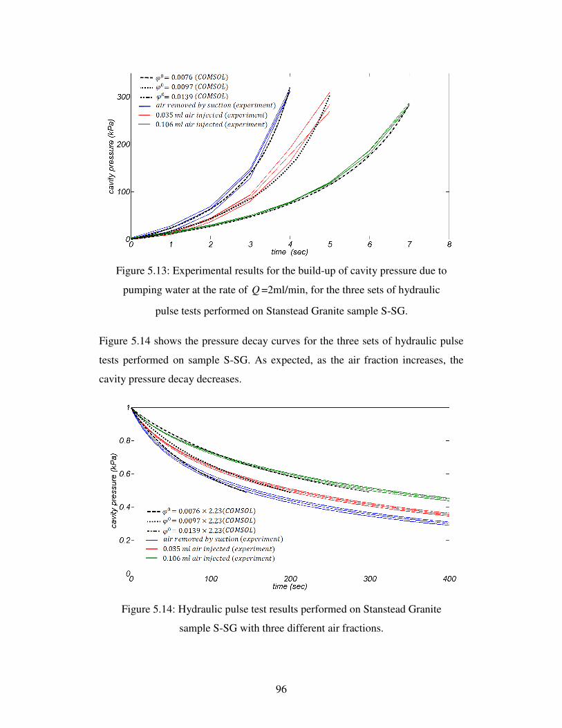
96


pumping water at the rate of Q =2ml/min, for the three sets of hydraulic

pulse tests performed on Stanstead Granite sample S-SG.

Figure 5.14 shows the pressure decay curves for the three sets of hydraulic pulse

tests performed on sample S-SG. As expected, as the air fraction increases, the

cavity pressure decay decreases.


sample S-SG with three different air fractions.

97

The measured fluid pressure curves were then fitted using COMSOLTM. A

permeability of 3.6 ×10-18 m2 best fitted the results of the three sets of test for the

first 50% pressure drop.

5.5. Permeability measurement of the large sample

A large sample of Stanstead Granite, L-SG, was also tested to measure the

permeability using both steady state and hydraulic pulse testing techniques. The

diameter of the sample was 152.4 mm with a height of 304.8 mm. The sample

contained a central cavity partially drilled along the central axis of the sample

with a diameter of 25.4 mm and a height of 152.4 mm. The bottom surface of the

sample, which was drilled through, was sealed using BondoTM fibreglass resin.

Hence, sample L-SG had flow boundary conditions similar to the smaller sample

S-SG, which was tested previously. The L-SG sample was saturated in a vacuum

chamber for a week.

In order to minimize the amount of air bubbles trapped in the central cavity of the

sample, it was placed in the experimental container in a large water tank while

both the container and the sample were submerged. Sealing between the epoxy-

coated sample surface and the bottom plate was provided using an O-ring. The

sealing pressure on the O-ring was 3 MPa, which was sufficient to provide the

sealing. Vacuum grease was also used on the O-ring surface to ensure better

sealing conditions. Figure 5.15 is a schematic of the sample and the testing

facility. The sealing pressure was measured using a 45 kN FutekTM load cell. The

cavity pressure was measured using a 1400 kPa Honeywell pressure transducer.

The total cavity volume (the drilled part of the sample and the connections and

fittings) was 98.2 cm3.

98

Figure 5.15: A schematic view of the setup used for measuring the

permeability of Stanstead Granite sample L-SG.

5.5.1. Steady state tests

A set of steady state tests was performed on the sample, using a QuizixTM

precision pump to apply flow rates of 0.025, 0.05, 0.1, and 0.15 ml/min. Table 5.2

gives the measured data and the corresponding permeability values estimated at

each flow rate. The estimated permeability for the tested sample was (5.35 to

5.48) ×10-18 m2. Figure 5.16 shows the change of cavity pressure with respect to

time. The problem was also modelled in COMSOLTM.

Table 5.2. The results of steady state tests performed on the large sample of

Stanstead Granite, L-SG.

Point 1 2 3 4

Q (ml/min) 0.025 0.05 0.1 0.15

p (kPa) 125.9 246.5 495.5 741.9

K% (m2) 5.35×10-18 5.48×10-18 5.44×10-18 5.44×10-18

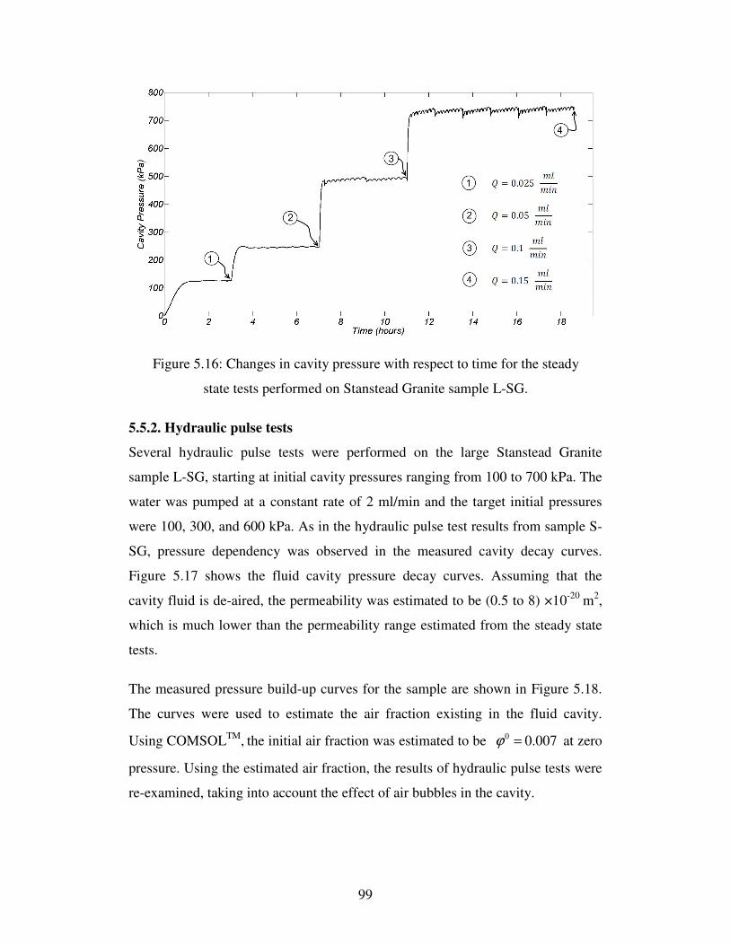
99

Figure 5.16: Changes in cavity pressure with respect to time for the steady

state tests performed on Stanstead Granite sample L-SG.

5.5.2. Hydraulic pulse tests

Several hydraulic pulse tests were performed on the large Stanstead Granite

sample L-SG, starting at initial cavity pressures ranging from 100 to 700 kPa. The

water was pumped at a constant rate of 2 ml/min and the target initial pressures

were 100, 300, and 600 kPa. As in the hydraulic pulse test results from sample S-

SG, pressure dependency was observed in the measured cavity decay curves.

Figure 5.17 shows the fluid cavity pressure decay curves. Assuming that the

cavity fluid is de-aired, the permeability was estimated to be (0.5 to 8) ×10-20 m2,

which is much lower than the permeability range estimated from the steady state

tests.

The measured pressure build-up curves for the sample are shown in Figure 5.18.

The curves were used to estimate the air fraction existing in the fluid cavity.

Using COMSOLTM, the initial air fraction was estimated to be 0 0.007ϕ = at zero

pressure. Using the estimated air fraction, the results of hydraulic pulse tests were

re-examined, taking into account the effect of air bubbles in the cavity.

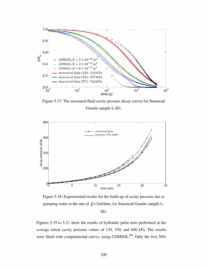
100

Figure 5.17: The measured fluid cavity pressure decay curves for Stanstead

Granite sample L-SG.


pumping water at the rate of Q =2ml/min, for Stanstead Granite sample L-

SG.

Figures 5.19 to 5.21 show the results of hydraulic pulse tests performed at the

average initial cavity pressure values of 130, 330, and 640 kPa. The results

were fitted with computational curves, using COMSOLTM. Only the first 50%

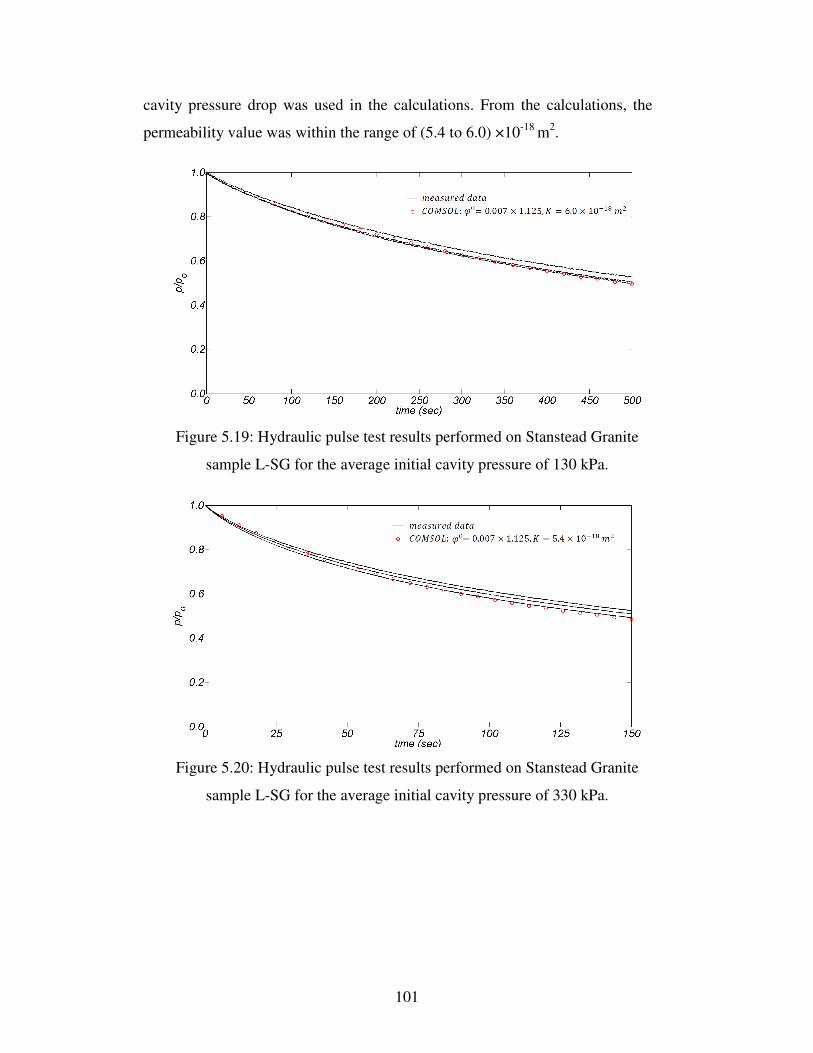
101

cavity pressure drop was used in the calculations. From the calculations, the

permeability value was within the range of (5.4 to 6.0) ×10-18 m2.


sample L-SG for the average initial cavity pressure of 130 kPa.



102



5.6. Summary

In this chapter, a technique was proposed to correct for effects caused by the

existence of air bubbles in the sealed cavity used in hydraulic pulse testing. Since,

in practice, it is impossible to remove all the air bubbles from a sealed cavity,

their effect should be taken into account. A relationship was presented to calculate

the compressibility of the air-water mixture. It has been observed in the literature

that the existence of 1% of air in the water increases the compressibility by three

orders of magnitude. It was suggested that the amount of trapped air in the fluid

cavity can be estimated from the pressure build-up curve. If the flow rate to the

cavity is high enough, the pressure build-up becomes independent of the

permeability of the rock. A series of steady state tests was performed on two

different samples of Stanstead Granite by applying increasing flow rates. The

permeability was measured to be within the range of (3.45 to 5.48) ×10-18 m2 and

no pressure dependency was observed in the permeability measurement.

However, the hydraulic pulse decay curves were highly dependent on the initial

cavity pressure, which can only be explained by the pressure dependency of water

compressibility. The relationship between the compressibility of the cavity fluid

and the cavity pressure was back-calculated from the pressure build-up stage of

the hydraulic pulse test. It was seen that using the compressibility of pure water to

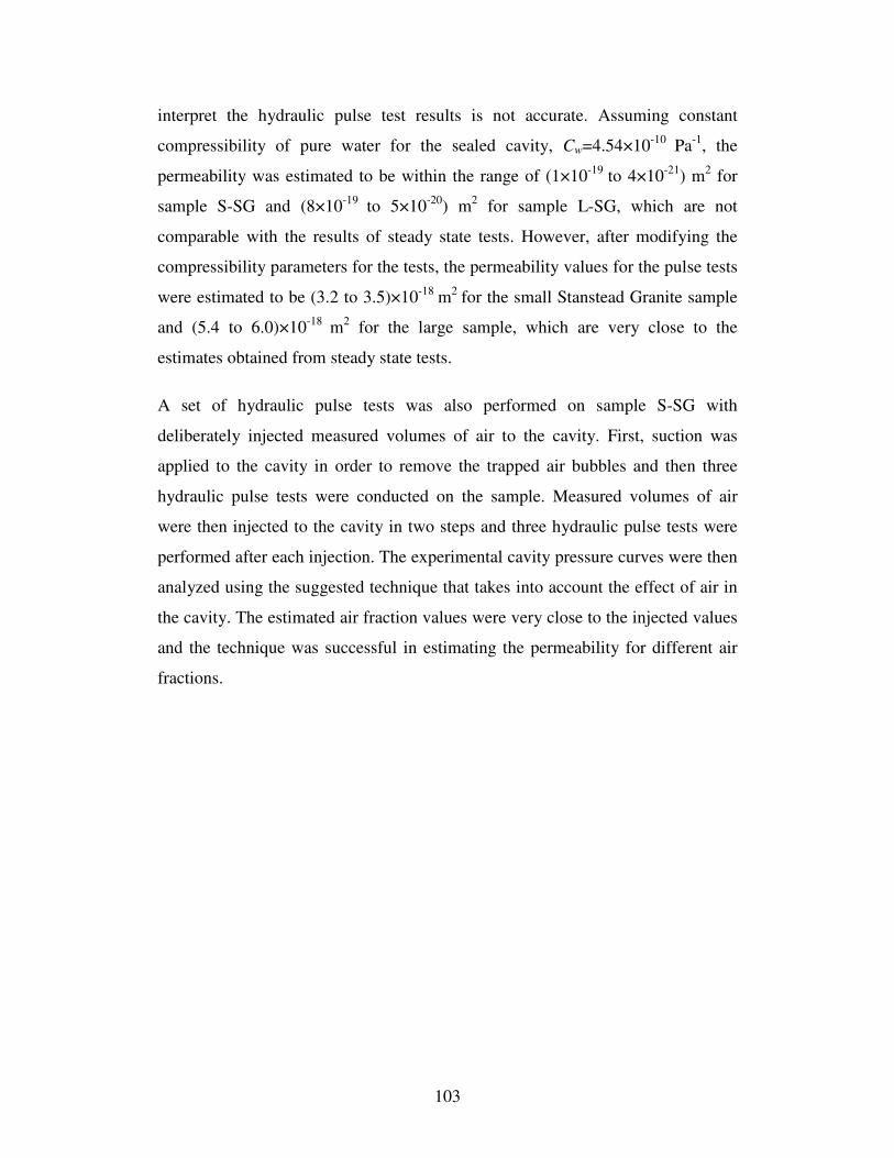
103

interpret the hydraulic pulse test results is not accurate. Assuming constant

compressibility of pure water for the sealed cavity, Cw=4.54×10-10 Pa-1, the

permeability was estimated to be within the range of (1×10-19 to 4×10-21) m2 for

sample S-SG and (8×10-19 to 5×10-20) m2 for sample L-SG, which are not

comparable with the results of steady state tests. However, after modifying the

compressibility parameters for the tests, the permeability values for the pulse tests

were estimated to be (3.2 to 3.5)×10-18 m2 for the small Stanstead Granite sample

and (5.4 to 6.0)×10-18 m2 for the large sample, which are very close to the

estimates obtained from steady state tests.

A set of hydraulic pulse tests was also performed on sample S-SG with

deliberately injected measured volumes of air to the cavity. First, suction was

applied to the cavity in order to remove the trapped air bubbles and then three

hydraulic pulse tests were conducted on the sample. Measured volumes of air

were then injected to the cavity in two steps and three hydraulic pulse tests were

performed after each injection. The experimental cavity pressure curves were then

analyzed using the suggested technique that takes into account the effect of air in

the cavity. The estimated air fraction values were very close to the injected values

and the technique was successful in estimating the permeability for different air

fractions.

104

CHAPTER 6

PERMEABILITY HYSTERESIS UNDER ISOTROPIC COMPRESSION

6.1. Introduction

The evolution of permeability in Stanstead Granite under isotropic compressive

loading and unloading was experimentally studied. In a practical application, the

granite is under overburden stresses. For instance, the in situ isotropic stress state

on a granite sample located at a depth of 1000 meters is estimated to be in the

range of 24 MPa to 27 MPa, whereas a sample recovered from the same depth is

generally regarded as unstressed. Therefore, it can be expected that the hydro-

mechanical behaviour of the rock measured in the laboratory will be different

from in situ behaviour. The increase of isotropic stresses in homogeneous rocks

tends to close fissures, micro-cracks and the pore space. The expected result is a

decrease in permeability, and an increase in Young’s modulus and Poisson’s ratio.

Depending on the applied stress level, the changes in the hydro-mechanical

parameters can be partially or completely recovered after unloading. The changes

of permeability in granitic rocks under isotropic compression have been studied

by a number of researchers, including Brace et al. (1968), Kranz et al. (1979),

Heystee and Roegiers (1981), and Kiama et al. (1996).

105

In this chapter, the alteration of permeability in three Stanstead Granite cylinders,

measuring approximately 100 mm in diameter and 100 mm in height, was studied.

All of the samples were cored from the same rock slab; two of them were cored

perpendicular to the slab surface and one parallel to the surface. The permeability

of all three samples was tested under steady state conditions in a GDS Triaxial

Cell (manufactured by GDS Instruments Inc.).

6.2. Sample preparation

Three cylindrical samples of Stanstead Granite were tested: GDS1 measured 9.98

cm in diameter and 10.63 cm in length, GDS2 measured 9.98 cm in diameter and

10.62 cm in length and GDS3 measured 9.90 cm in diameter and 10.05 cm in

length. The samples were cored from the same granite slab. Samples GDS1 and

GDS2 were cored at an orientation vertical to the slab surface while sample GDS3

was cored at a horizontal orientation. The two ends of the cored samples were cut

using a diamond saw. The samples were then machined to obtain smooth surfaces

and parallel ends. Figure 6.1 shows the three samples and the slab from which the

samples were cored.

In order to examine the porosity of the samples, the dimensions were accurately

measured and the samples were then left in an oven at a temperature of 60 Co for

three days and the dry weight of the samples were measured. In order to saturate

the samples, they were placed under water in the vacuum chamber (i.e. Figure

6.2) with a negative pressure of 90 kPa and weighed daily; after three days of

saturation the weight remained unchanged. The samples, however, were kept in

the vacuum chamber for a week, the saturated samples were weighed and the

porosity of the samples was estimated. The average porosity value was

0.67% ± 0.02%.

106

Figure 6.1: (a) The Stanstead Granite slab that the specimens were cored

from; (b) the three Stanstead Granite cylinders used in the study of

permeability hysteresis under isotropic loading.

Figure 6.2: Schematic layout of the saturation chamber (after Selvadurai et

al., 2011).

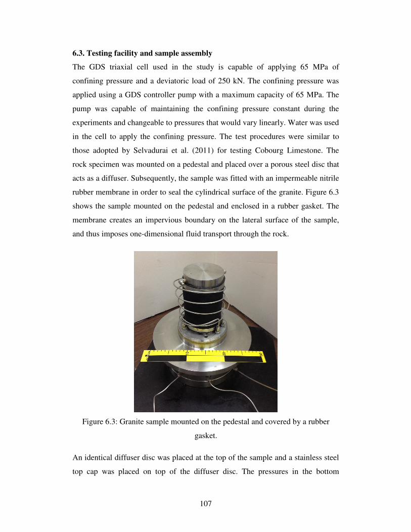
107

6.3. Testing facility and sample assembly

The GDS triaxial cell used in the study is capable of applying 65 MPa of

confining pressure and a deviatoric load of 250 kN. The confining pressure was

applied using a GDS controller pump with a maximum capacity of 65 MPa. The

pump was capable of maintaining the confining pressure constant during the

experiments and changeable to pressures that would vary linearly. Water was used

in the cell to apply the confining pressure. The test procedures were similar to

those adopted by Selvadurai et al. (2011) for testing Cobourg Limestone. The

rock specimen was mounted on a pedestal and placed over a porous steel disc that

acts as a diffuser. Subsequently, the sample was fitted with an impermeable nitrile

rubber membrane in order to seal the cylindrical surface of the granite. Figure 6.3

shows the sample mounted on the pedestal and enclosed in a rubber gasket. The

membrane creates an impervious boundary on the lateral surface of the sample,

and thus imposes one-dimensional fluid transport through the rock.

Figure 6.3: Granite sample mounted on the pedestal and covered by a rubber

gasket.

An identical diffuser disc was placed at the top of the sample and a stainless steel

top cap was placed on top of the diffuser disc. The pressures in the bottom

108

pedestal and the top cap are separately controllable through the stainless steel

lines rated for 65 MPa pressure and accessible from the outside the GDS cell.

Figure 6.4 shows the GDS cell and the connections. In order to improve the

sealing at the pedestal-membrane interface and the top cap-membrane interface

hose clamps were used for each end of the sample, a technique that has proved to

be effective (Selvadurai and Glowacki, 2008; Selvadurai et al., 2011a). Also, to

further reduce leakage from the cell to the top and the bottom of the sample

SikaTM sealant was applied at the interface of the nitrile gasket and the stainless

steel top and bottom caps. The sealant provided a continuous sealing. The

efficiency of the sealing technique and the apparent permeability of the system

was examined by Selvadurai et al. (2011a) using an aluminum cylinder on the test

specimen; from their results the leakage of the system was equivalent to

permeability of 3.0×10-23 (m2).

Figure 6.4: Schematic view of the GDS cell used for performing the

permeability hysteresis tests on Stanstead Granite (from Glowacki, 2008).

109

A QuizixTM pump provided flow through the samples. Three pressure transducers

were used to measure the water pressure; a 68 MPa OmegaTM pressure transducer

to measure the cell pressure and another 68 MPa OmegaTM pressure transducer to

measure the water pressure at the upstream.

6.4. Steady-state permeability measurement

The sample was subjected to a cell pressure with complete drainage allowed to

occur. Water was then pumped into the samples at a constant flow rate while

subjecting them to different confining pressures during the loading and unloading

stages. The water pressure at the upstream boundary that was required to keep the

flow rate constant was recorded during the tests. The downstream was kept open

to the atmosphere. Once the system reached a steady state, the pressure attained at

the upstream boundary was recorded and the steady state permeability of the

granite sample was calculated for the different values of confining pressure.

Figure 6.5 shows the schematic layout of the testing setup.

Employing Darcy’s Law for the one-dimensional steady state flow through a

cylindrical porous rock, the relationship for the permeability can be written as

2

QLK

r p

µ

π=

∆% (6.1)

where K% is the permeability parameter, Q is the flow rate at a steady state

condition, µ is the dynamic viscosity of permeating fluid at test temperature, L is

the length of the cylindrical sample, r is the radius of the cross section of the

sample, and p∆ is the pressure difference between the two ends of the sample

under steady state conditions.

110

Figure 6.5: The schematic arrangement of the setup used for steady state

permeability measurement of cylindrical Stanstead Granite samples

subjected to confining pressure (from Selvadurai et al. (2011)).

6.4.1. Steady state test results

A constant flow rate of 0.0050 ml/min was applied to the first sample, GDS1,

under varying confining pressures of 5, 10, 20 and 30 MPa. The time for

attainment of a steady state was approximately 10 hours for the lowest

permeability. The sample was subsequently unloaded to confining pressures of

20, 10 and 5 MPa. A single test was performed at each confining pressure. Table

6.1 shows the results of the experiments performed on sample GDS1.

For the second specimen, GDS2, a constant flow rate of 0.0010 ml/min was

applied to the sample under confining pressures of 5, 10, 20, 30 and 40 MPa. The

constant flow rate was then reduced to 0.0005 ml/min for the test at 50 MPa and

further reduced to 0.0002 ml/min for the test at 60 MPa, in order to keep the

upstream cavity pressure low. The sample was finally unloaded under similar

confining stresses and flow rates. It should be noted that for the second specimen

(i.e. GDS2), the tests were repeated three times for each confining pressure and

the maximum steady state pressure difference was 5.8%. The results are shown in

Table 6.2.

111

Table 6.1: Steady state permeability tests on Stanstead Granite sample

GDS1 at various confining pressures.

Sample GDS3 was tested at confining pressures of 5, 10, 20, 40, 60, 40, 20, 10, 5

kPa. A flow rate of 0.0002 ml/min was applied to the sample at all cell pressures,

except for the 60 MPa cell pressure and 40 MPa cell pressure in the unloading

stage, which were tested at a flow rate of 0.0001 ml/min. Since the measured

permeability for sample GDS3 at the 60 MPa cell pressure was much lower than

the corresponding value for sample GDS2, a constant pressure steady state test

was also performed at this cell pressure on sample GDS3, in order to verify the

estimated permeability. The base of the sample was subjected to the constant

pressure of 1MPa and the pore pressure at the top end of the sample was kept

open to atmospheric pressure. The decrease in the flow rate supplied by the pump

that was necessary to keep the pressure boundary condition constant was

monitored. The sample reached a steady state condition after 8 days, at a flow rate

of 1.6×10-5 ml/min. The so-called pressure and flow boundary conditions

correspond to a permeability of 3.3×10-21 m2, which confirmed the estimated

permeability value at a constant flow rate. Table 6.3 shows the results of the

steady state tests performed on sample GDS3.

Cell Pressure (MPa)

Flow Rate

(ml/min)

Steady State

Pressure (kPa)

Steady State Permeability

(m2)

5 0.0050 681 15×10-19

10 0.0050 1650 6.3×10-19

20 0.0050 4130 2.5×10-19

30 0.0050 8238 1.3×10-19

20 0.0050 4936 2.1×10-19

10 0.0050 2184 4.7×10-19

5 0.0050 1039 9.9×10-19

112

Table 6.2: Steady state permeability of Stanstead Granite sample GDS2 at

different confining pressures.

Cell Pressure (MPa)

Flow Rate

(ml/min)

Steady State Pressure (kPa)

Steady State Permeability (m2)

Test 1 Test 2 Test 3 Test 1 Test 2 Test 3 Average

5 0.001 172 168 172 1.2×10-18 1.2×10-18 1.2×10-18 1.2×10-18 10 0.001 330 350 339 6.3×10-19 5.9×10-19 6.1×10-19 6.1×10-19 20 0.001 941 944 967 2.2×10-19 2.2×10-19 2.1×10-19 2.2×10-19 30 0.001 2604 2666 2649 7.9×10-20 7.7×10-20 7.8×10-20 7.8×10-20 40 0.001 4637 4741 4871 4.5×10-20 4.4×10-20 4.2×10-20 4.3×10-20 50 0.0005 4272 4295 4518 2.4×10-20 2.4×10-20 2.3×10-20 2.4×10-20

60 0.0002 3138 3235 3167 1.3×10-20 1.3×10-20 1.3×10-20 1.3×10-20

50 0.0005 5845 5817 6058 1.8×10-20 1.8×10-20 1.7×10-20 1.8×10-20

40 0.001 7854 7786 7761 2.6×10-20 2.7×10-20 2.7×10-20 2.6×10-20

30 0.001 5338 5391 5357 3.9×10-20 3.8×10-20 3.9×10-20 3.9×10-20 20 0.001 2782 2752 2759 7.4×10-20 7.5×10-20 7.5×10-20 7.5×10-20 10 0.001 943 985 928 2.2×10-19 2.1×10-19 2.2×10-19 2.2×10-19 5 0.001 410 399 417 5.1×10-19 5.2×10-19 5.0×10-19 5.1×10-19

Table 6.3: Steady state permeability of Stanstead Granite sample GDS3 at

different confining pressures.

Cell Pressure (MPa)

Flow Rate

(ml/min)

Steady State Pressure (kPa)

Steady State Permeability (m2)

5 0.0002 43 9.6×10-19

10 0.0002 79 5.3×10-19

20 0.0002 348 1.2×10-19

40 0.0002 1004 4.1×10-20

60 0.0001 5750 3.6×10-21

40 0.0001 3044 6.8×10-21

20 0.0002 1887 2.2×10-20

10 0.0002 550 7.5×10-20

5 0.0002 205 2.0×10-19

113

6.4.2. Discussion on the steady state test results

Figure 6.6 shows the change in permeability for the three samples tested with

respect to the change in the confining pressure. The permeability of sample GDS1

reduced from 1.5×10-18 m2 to 1.3×10-19 m2 while the confining pressure increased

from 5 MPa to 30 MPa. The permeability was then increased to 9.9×10-19 m2 as

the confining pressure was reduced to 5 MPa. For sample GDS2 which was

loaded up to 60 MPa cell pressure, the permeability decreased from 1.2×10-18 m2

to 1.3×10-20 m2. The permeability at the end of the unloading stage (e.g. 5 MPa

cell pressure) was 5.1×10-19 m2. Finally, the measured permeability for sample

GDS3 reduced from 9.6×10-19 m2 to 3.6×10-21 m2 for, respectively, 5 and 60 MPa

in the loading stage and increased to 2.0×10-19 m2 at 5 MPa in the unloading stage.

It can be seen that part of the permeability decrease in the loading stage is due to

the elastic contraction of the pores, fissures and micro-cracks and part of it is due

to permanent closure of micro-cracks and the collapse of pores.

Figure 6.6: The change of permeability with an isotropic compression

change for Stanstead Granite samples GDS 1, GDS 2 and GDS 3.

As expected, the maximum of 30 MPa isotropic compression in sample GDS1 had

less permanent permeability decrease than the maximum 60 MPa isotropic

compression on samples GDS2 and GDS3. Also, a comparison of the

114

permeability results from samples GDS2 and GDS3 shows anisotropy both in the

permeability and in the evolution of damage under isotropic loading-unloading

cycles. Therefore, not only the permeability evolves but also the degree of

anisotropy changes. Table 6.4 shows the change in the permeability anisotropy for

samples GDS2 and GDS3.

Table 6.4: Change in the degree of anisotropy ( 2 3GDS GDSK K ) with the

change of isotropic compression.

Regarding any leakage from the system, since the minimum estimated

permeability value was 3.6 ×10-21 m2, which is two orders of magnitude higher

than the apparent permeability of the system, no correction was needed.

6.5. Summary

In this chapter, the evolution of permeability in Stanstead Granite was studied

under the effects of isotropic loading and unloading. Three cylindrical samples

were tested in a triaxial cell, using the steady state technique. Two samples were

cored with their cylindrical axis perpendicular to the granite slab (i.e. samples

GDS1 and GDS2) and one sample was cored with the axis parallel to the surface

of the slab (i.e. GDS3). The loading-unloading cycle ranged from confining

stresses of 5 MPa to 30 MPa for sample GDS1 and 5 MPa to 60 MPa for samples

GDS2 and GDS3. The isotropic loading decreased the permeability value by

almost one order of magnitude for sample GDS1 and two to three orders of

magnitude for samples GDS2 and GDS3. The permeability decrease is most likely

to be attributed to the closure of the accessible pore space. The permeability was

partially recovered when the sample was completely unloaded. The irrecoverable

decrease in the permeability after one loading-unloading cycle, although

negligible, can result from permanent pore closure during isotropic loading. Also,

Loading Unloading Cell Pressure

(MPa) 5 10 20 40 60 40 20 10 5

Degree of anisotropy

1.25 1.15 1.83 1.04 3.61 3.82 3.41 2.93 2.55

115

a comparison of the permeability evolution in samples GDS2 and GDS3 showed

isotropic hydraulic properties until the increase of cell pressure from 40MPa to 60

MPa; at these cell pressures the permeability parallel to the surface of the slab

became almost 3 times less than the permeability perpendicular to the surface of

the slab.

116

CHAPTER 7

THERMO-HYDRO-MECHANICS OF POROUS GEOMATERIALS

7.1. Introduction

The thermo-hydro-mechanical behaviour of porous media is an extension to

Biot’s theory of poroelasticity (Biot, 1941a) that has been studied extensively

both theoretically and experimentally (Mandel, 1953; Cryer, 1963; Gibson et al.,

1963, Mason et al., 1991; Wang, 2000; Selvadurai, 2007). In a variety of

problems such as deep geological disposal of nuclear wastes (Selvadurai and

Nguyen, 1995; Selvadurai and Nguyen, 1997; Tsang et al. 2000; Zimmerman,

2000; Rutqvist et al., 2001; Stephansson et al., 2004; Alonso et al., 2005;

Chijimatsu et al., 2005; Nguyen et al., 2005; Rutqvist et al., 2005; Selvadurai and

Suvorov, 2012; Tsang et al., 2012), oil and natural gas recovery (Vaziri, 1988; Bai

and Roegiers, 1994; Gutierrez and Makurat, 1997; Pao et al., 2001) and

geothermal energy extraction (Brownell et al., 1977; Bodvarsson and Stefansson,

1989; Nakao and Ishido, 1998; Ilyasov et al., 2010), the role of temperature

becomes important. Biot’s isothermal theory of poroelasticity was extended by a

number of researchers in order to include non-isothermal effects; examples of

these developments are given by Noorishad et al. (1984), Booker and Savvidou

(1984, 1985), Aboustit et al. (1985), McTigue (1986), Coussy (1989), Selvadurai

and Nguyen (1995), Zhou et al. (1998), Gens et al. (1998), Pao et al. (2001),

117

Suvorov and Selvadurai (2010) and Selvadurai and Suvorov (2012). In this

chapter the coupling effects of temperature, pore pressure and skeletal

deformations are investigated. Experimental research involves the heating of

Stanstead Granite cylinders each containing a fluid inclusion is performed to

establish the applicability of currently available THM formulation.

7.2. Governing Equations

In this section, the partial differential equations for the thermo-hydro-mechanical

behavior of porous geomaterials are summarized for completeness.

7.2.1. The constitutive equation for the porous solid

Temperature change induces volumetric deformation and, subsequently, isotropic

stress in the porous skeleton. This effect can be implemented in Hooke’s stress-

strain relationship by adding the volumetric thermal expansion

2 v sG p KTλε α β= + − −I I Iσ εσ εσ εσ ε (7.1)

where G is the linear elastic shear modulus, λ is the Lamé coefficient, εεεε is the

strain tensor, vε ( tr= εεεε ) is the volumetric strain, sβ is the volumetric thermal

expansion coefficient of the solid material, K is the drained bulk modulus, T is the

temperature measured from a reference state and I is the unit tensor. Substituting

Eq. (7.1) into the equilibrium equation (i.e. Eq. (3.44)) and considering static

equilibrium in the absence of body forces gives the solid phase equation for non-

isothermal poroelastic materials:

2 ( . )1 2 s

GG p K Tα β

ν∇ + ∇ ∇ − ∇ − ∇ =

−u u 0 (7.2)

7.2.2. Liquid phase equation

Temperature change can affect the fluid flow in two ways: It changes the dynamic

viscosity, the volumetric thermal expansion coefficient and the density of the fluid

(Holzbecher, 1998); it also induces fluid flow due to the difference between

thermal expansion of fluid and the solid skeleton. The volumetric strain v

ε can be

118

written as a function of the mean total stress1

( tr )3

= σσσσ , pore pressure and

temperature; i.e.

vv s

pT

K H

σε β= + + (7.3)

where vσ is the mean total stress and H is the poroelastic expansion coefficient.

The increment of fluid content (i.e. (3.25)) can also be modified to include the

effect of temperature change

vT

p

H R

σξ ξ= + + (7.4)

where Tξ is the increment of fluid content induced by the temperature change.

Using the definition in Eq. (3.20) and the fact that the change in pore volume

under the temperature variation is the difference between the bulk volume change

and the volume change of solid grains (Selvadurai and Nguyen, 1995), Tξ can be

written as

( ) ( ) 1T T T

s f s s fT

V V V V T n V T nV T

V V

δ δ δ β β βξ

− − − − −= = (7.5)

where n is the porosity, fβ is the volumetric thermal expansion coefficient of the

permeating fluid and TVδ , T

sVδ , TfVδ are the temperature induced volume

change for, respectively, the bulk volume of the porous medium, the solid grains,

and the fluid. Substituting Eq. (7.5) into Eq. (7.4) gives

( )vs f

pn T

H R

σξ β β= + + − (7.6)

Substituting Eq. (7.6) into the mass conservation equation (i.e. Eq. (3.35)) gives

the non-isothermal fluid phase equation

119

( . ). ( ) ( ) 0

( ) f s

p K TS p n T n

t T t tε α β α β

µ

∂ ∂ ∇ ∂ + ∇ − ∇ + − + − = ∂ ∂ ∂

% u (7.7)

7.2.3. Energy equation

Heat transfer in porous media can take place through conduction, convection and

radiation. The radiation part of the heat transfer process is neglected. Convective

heat transfer is due to the bulk movement of the permeating fluid. Since the

current research is focused on the study of low permeability geomaterials where

the fluid flows at very low velocities, the effect of convection in heat transfer can

be neglected, compared to conduction. Employing Fourier’s Law for conductive

heat transfer gives

*T ck T= − ∇q (7.8)

where Tq is the heat flux, and *ck is the overall thermal conductivity of the

porous material. The overall thermal conductivity of the porous material can be

found as the volume average of the phase thermal conductivities

* (1 )= + −c cf csk nk n k (7.9)

where cfk and csk are the thermal conductivities of the liquid phase and solid

phase, respectively.

If the mechanical and fluid flow contributions to the energy balance are neglected,

the net rate of heat flux into any arbitrary element of material will be balanced by

the increase in internal heat energy (Savvidou and Booker, 1988)

*T ( ) 0p

Tc T

t

∂∇ + =

∂q (7.10)

where * ( )pc T is the specific heat capacity of the porous medium. The overall heat

capacity is defined as the volume average of the phase heat capacities

120

* ( ) ( ) (1 )p f f s sc T n T c n cρ ρ= + − (7.11)

where fc and sc are the specific heat capacity of the liquid phase and the solid

phase, respectively. Substituting Eq. (7.8) into Eq. (7.10) provides the conductive

heat transfer equation

* * 2( ) 0p c

Tc T k T

t

∂− ∇ =

∂ (7.12)

7.2.4. Computational modelling of a fluid inclusion

Since the measurement of fluid pressure and temperature in the sealed cavity is

experimentally feasible, the concept of a fluid inclusion was implemented in the

current research. The fluid inclusion was modelled as a porous medium with the

porosity equal to unity and a relatively high permeability in order to create

uniform pressure within the cavity (i.e. we set 6/ 10fK K−=% % ). Also, to capture the

effect of cavity volume change on the cavity pressure change, the elastic constants

were assumed to be 0.49f

ν = and 3(1 2 ) /f eq

E Cν= − , where eq

C is the

compressibility of the cavity fluid that contains trapped air. The equations used to

model the fluid cavity are as follows:

2( ) ( . ) 03

DGK G+ ∇ ∇ + ∇ =u u (7.13)

( . )

( ) . ( ) 0( )eq f

p K TC p p T

t T t tβ

µ

∂ ∂ ∇ ∂+ ∇ − ∇ + − =

∂ ∂ ∂

% u (7.14)

2( ) 0f f cf

TT c k T

tρ

∂− ∇ =

∂ (7.15)

In the above formulation, the compressibility of the fluid in the sealed cavity is

higher than the compressibility of de-aired water due to unwanted entrapment of

air bubbles in the fluid-filled cavity. Referred to Chapter 5, a simplified

relationship for the compressibility of an air-water mixture can be written as

121

(1 )eq a wC C Cϕ ϕ= + − (7.16)

where ϕ is the air fraction in the fluid-air mixture (volume of air/volume of fluid-

filled cavity), and Cw is the compressibility of the pure fluid, i.e. 4.54×10-10 Pa-1

(White, 1986). Expressions analogous to Eq. (7.16) that take into account air

solubility were also investigated in Chapter 5. For non-isothermal phenomena the

behaviour of the air bubbles follows the ideal gas law

.aPVnR

T= (7.17)

where aV is the volume of the air, P is absolute pressure of the air bubble, n is the

number of moles and R is the universal gas constant. Considering variations in Eq.

(7.17) we have

1 1a

aa a a

dV

V dTPdV V dP nRdT C

dP P T dp

−

+ = ⇒ = = − (7.18)

The ideal gas law also determines the changes of air fraction with pressure and

temperature. Assuming that the total volume of cavity (i.e. w a

V V+ ) is constant

during the THM experiment, the air fraction equation can be re-written as

00

0 0 0 00

0 0;

aa

a a a a a a a

w a w a a

P TV

P V PV V P T P T

T T V V V V P Tϕ ϕ ϕ= = ⇒ = =

+ + (12)

where 0a

P is the initial absolute air pressure, 0aV is the initial volume of air, 0T is

the reference temperature and 0ϕ is the initial air fraction in the cavity.

The other important factor in the compressibility of the air-water mixture is the

dissolution of air into water. As stated in Henry’s Law, the weight of air that goes

into solution depends on the absolute pressure of the air. Based on Henry’s Law,

the volume of air present in water at 25 °C can be approximately 1.78% of the

122

volume of water (Fredlund, 1976). Also, the rate of dissolution depends on the

diffusivity rate of the air into water, which is governed by Fick’s Law. The

diffusivity rate for air in water is 2.0×10-9 m2/s at 25 °C. Depending upon the rate

of compression of an air-water mixture, the amount of air going into solution

changes from 0 to (1 )h ϕ− of the volume of water, where h is Henry’s constant.

Eq. (7.16) is a highly simplified relationship for estimating the compressibility of

the air-water mixture and does not take into account the effect of water vapor

pressure, surface tension and the time dependency for dissolution of air in the

water.

In addition to Eq. (7.16), which was obtained based on physical phenomena, an

empirical relationship that relates the compressibility of the air-fluid mixture to

pore pressure was suggested

( )-1( ) coteqC p A Bp= (7.19)

where A and B are empirical parameters that can be obtained from isothermal

hydraulic pulse tests. In this chapter both the air-water compressibility

relationships Eq. (7.16) and Eq. (7.19) are implemented in the modelling of the

THM experiments.

7.3. Thermal damage experiment

Any sudden temperature change can induce damage in porous geomaterials. Two

main reasons can be attributed to this damage: (i) the difference in the thermal

expansion coefficient of the minerals in the compound, (ii) a sudden pore pressure

increase in low permeability saturated geomaterials. The temperature range used

in the experiments performed in current research was between 20 o C to 70 o C ,

where minimal thermal damage is expected. However, an experiment was

performed to further investigate the issue. In this regard, the permeability of a

Stanstead Granite cylinder was measured, using the steady state technique, both

before and after a thermal shock.

123

7.3.1. Testing procedure

A cylindrical sample of Stanstead Granite measuring 15.24 cm in diameter and

30.48 cm in length was saturated in a vacuum chamber. The patch permeameter

described in section 4.3.2 was used to perform steady state tests on the upper and

lower plane surfaces of the sample. The details of the testing facility were

explained in Section 4.3.2. A schematic cross section of the sample and the

permeameter as well as a picture of the components of the assembly is presented

in Figure 7.1. The sample was vacuum saturated for 7 days and then moved to the

testing chamber for measuring its permeability prior to thermal shock.

Figure 7.1: Cross section of the permeameter connected to the sample

surface and the components of the assembly.

A sealing pressure of 1.5 MPa was applied to the gasket. A Quizix pump was

connected to the inlet of the permeameter and it delivered a constant flow rate of

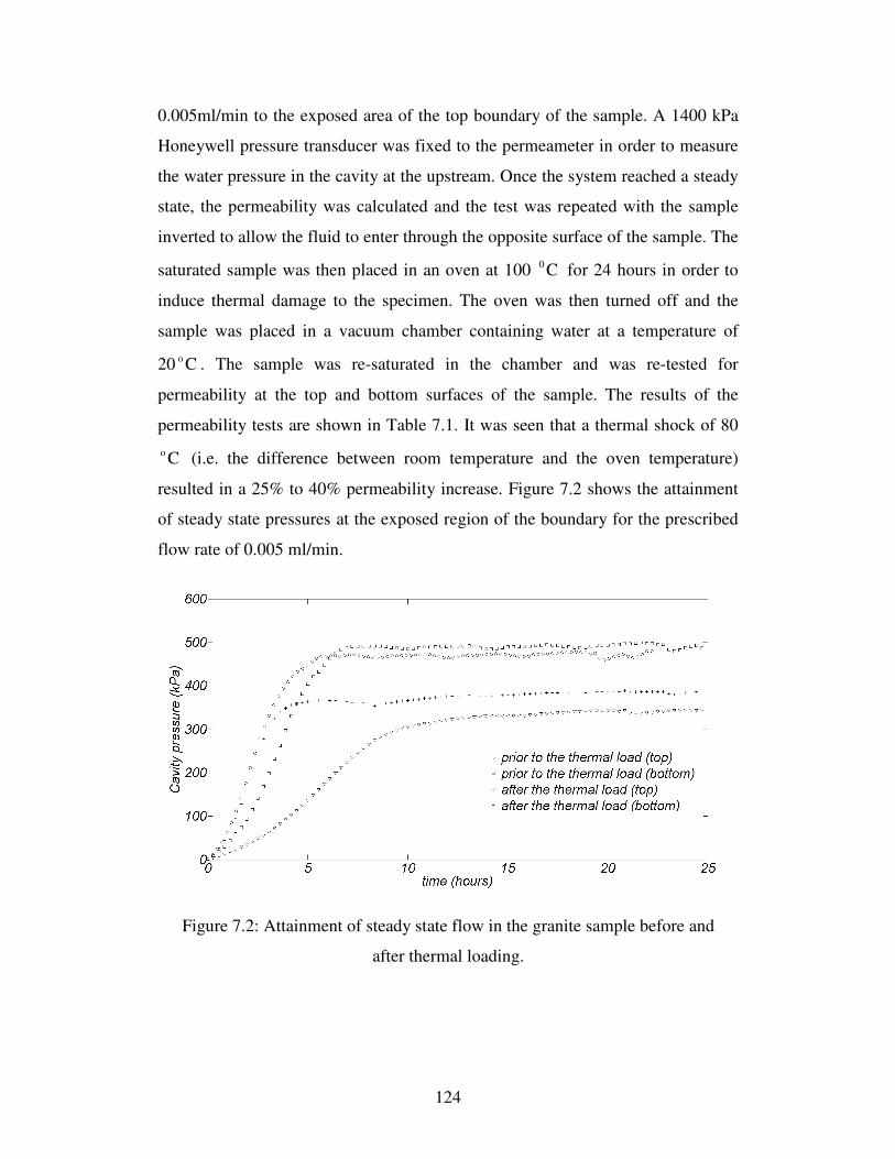
124

0.005ml/min to the exposed area of the top boundary of the sample. A 1400 kPa

Honeywell pressure transducer was fixed to the permeameter in order to measure

the water pressure in the cavity at the upstream. Once the system reached a steady

state, the permeability was calculated and the test was repeated with the sample

inverted to allow the fluid to enter through the opposite surface of the sample. The

saturated sample was then placed in an oven at 100 0 C for 24 hours in order to

induce thermal damage to the specimen. The oven was then turned off and the

sample was placed in a vacuum chamber containing water at a temperature of

20 o C . The sample was re-saturated in the chamber and was re-tested for

permeability at the top and bottom surfaces of the sample. The results of the

permeability tests are shown in Table 7.1. It was seen that a thermal shock of 80

o C (i.e. the difference between room temperature and the oven temperature)

resulted in a 25% to 40% permeability increase. Figure 7.2 shows the attainment

of steady state pressures at the exposed region of the boundary for the prescribed

flow rate of 0.005 ml/min.

Figure 7.2: Attainment of steady state flow in the granite sample before and

after thermal loading.

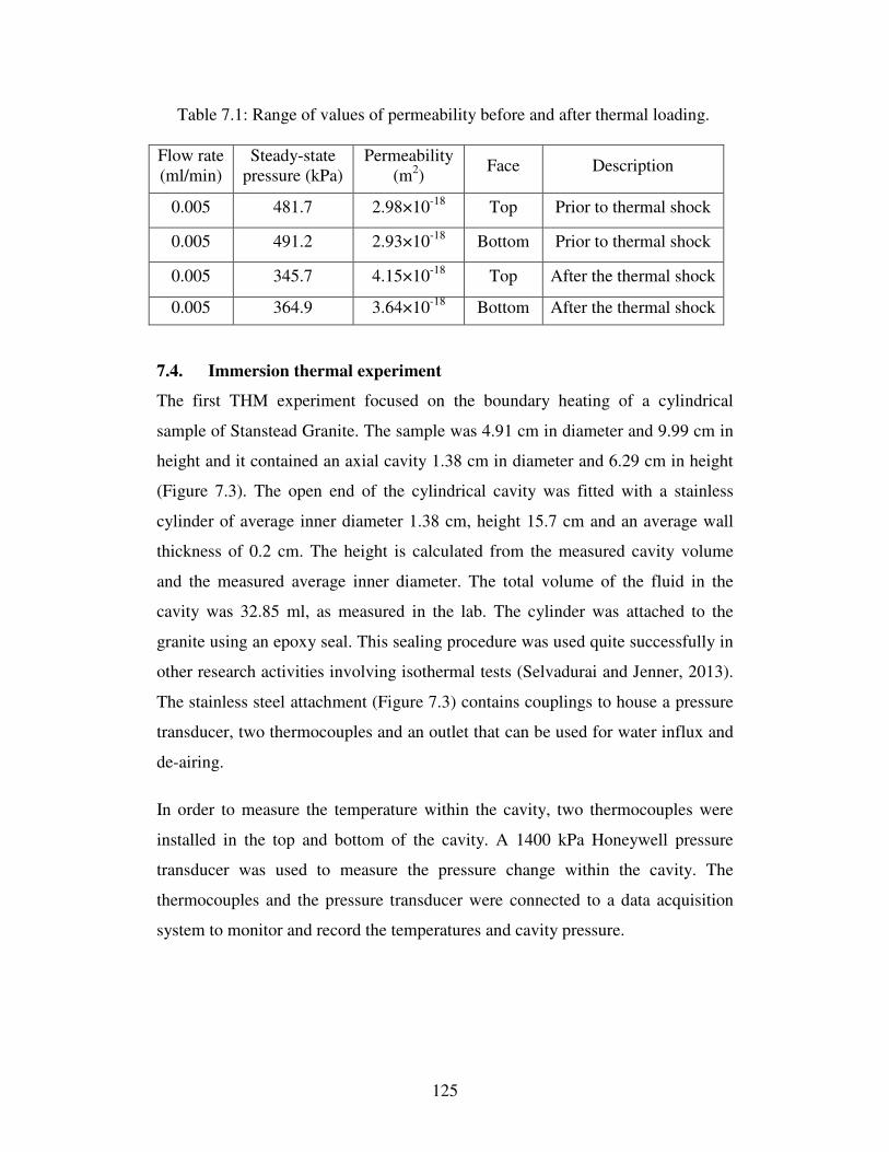
125

Table 7.1: Range of values of permeability before and after thermal loading.

Flow rate (ml/min)

Steady-state pressure (kPa)

Permeability (m2)

Face Description

0.005 481.7 2.98×10-18 Top Prior to thermal shock

0.005 491.2 2.93×10-18 Bottom Prior to thermal shock

0.005 345.7 4.15×10-18 Top After the thermal shock

0.005 364.9 3.64×10-18 Bottom After the thermal shock

7.4. Immersion thermal experiment

The first THM experiment focused on the boundary heating of a cylindrical

sample of Stanstead Granite. The sample was 4.91 cm in diameter and 9.99 cm in

height and it contained an axial cavity 1.38 cm in diameter and 6.29 cm in height

(Figure 7.3). The open end of the cylindrical cavity was fitted with a stainless

cylinder of average inner diameter 1.38 cm, height 15.7 cm and an average wall

thickness of 0.2 cm. The height is calculated from the measured cavity volume

and the measured average inner diameter. The total volume of the fluid in the

cavity was 32.85 ml, as measured in the lab. The cylinder was attached to the

granite using an epoxy seal. This sealing procedure was used quite successfully in

other research activities involving isothermal tests (Selvadurai and Jenner, 2013).

The stainless steel attachment (Figure 7.3) contains couplings to house a pressure

transducer, two thermocouples and an outlet that can be used for water influx and

de-airing.

In order to measure the temperature within the cavity, two thermocouples were

installed in the top and bottom of the cavity. A 1400 kPa Honeywell pressure

transducer was used to measure the pressure change within the cavity. The

thermocouples and the pressure transducer were connected to a data acquisition

system to monitor and record the temperatures and cavity pressure.

126

Figure 7.3: Geometry of the Stanstead Granite sample (dimensions are in

cm). The thermally insulated parts are shown as dashed lines.

7.4.1. Permeability measurement

Two sets of isothermal tests were performed on the granite sample, in order to

estimate the permeability and to calibrate the parameters used to estimate the

compressibility of the cavity fluid (i.e. Eq. (7.19)). Each test began with pumping

water at a constant rate into the cavity, giving sufficient time for the pressure to

reach a steady state condition. The pressure attained at steady state condition was

used to estimate the permeability value. The outlet valve of the cavity was then

closed, allowing the excess pore pressure to decay. This testing procedure was

primarily designed to calibrate Eq. (7.19) and is different from the conventional

hydraulic pulse testing procedure since the sample tested usually has no residual

pore pressure prior to cavity pressurization. Each set of experiments was repeated

three times in order to ensure the repeatability of the results. The flow rates used

were 0.01 ml/min and 0.02 ml/min. Figures 7.4 and 7.5 show the two sets of

hydraulic pulse tests. COMSOL MultiphysicsTM software was used to model the

complete experimental procedure and calibrate Eq. (7.19). Details of modelling

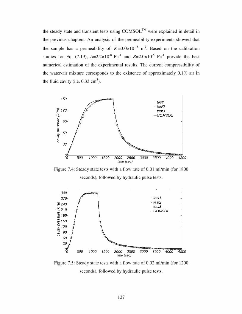
127

the steady state and transient tests using COMSOLTM were explained in detail in

the previous chapters. An analysis of the permeability experiments showed that

the sample has a permeability of K% =3.0×10-18 m2. Based on the calibration

studies for Eq. (7.19), A=2.2×10-8 Pa-1 and B=2.0×10-5 Pa-1 provide the best

numerical estimation of the experimental results. The current compressibility of

the water-air mixture corresponds to the existence of approximately 0.1% air in

the fluid cavity (i.e. 0.33 cm3).

Figure 7.4: Steady state tests with a flow rate of 0.01 ml/min (for 1800

seconds), followed by hydraulic pulse tests.


seconds), followed by hydraulic pulse tests.

128

7.4.2. Thermo-hydro-mechanical experiment

In order to study the transport of heat and fluid induced by temperature change,

the experimental setup shown in Figure 7.6 was prepared. The sample was

immersed in a water bath at a constant temperature of 50 ºC, while the outlet

valve of the fluid cavity was closed. The water temperature was kept constant

using a temperature controller connected to an electrical heater and a

thermocouple to measure the temperature of the water in the bath. The sample

was kept in the hot water bath for 3600 seconds and then rapidly removed from

the hot water bath and immersed into a cold water bath with a constant

temperature of 20ºC and kept there for 7200 seconds.

Figure 7.6: Schematic view of the thermo-hydro-mechanical experimental

setup.

The experimental cycle, including both heating and cooling steps, was repeated

six times in order to study the hysteretic behaviour of the material. It should be

noted that each new testing cycle was started after sufficient time was allowed for

the dissipation of residual pore pressure and temperature from the previous cycle.

As mentioned in Section 7.4, the cavity fluid pressure and cavity fluid

temperature were recorded using a pressure transducer and two thermocouples.

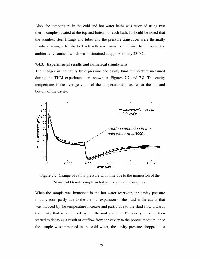
129

Also, the temperature in the cold and hot water baths was recorded using two

thermocouples located at the top and bottom of each bath. It should be noted that

the stainless steel fittings and tubes and the pressure transducer were thermally

insulated using a foil-backed self adhesive foam to minimize heat loss to the

ambient environment which was maintained at approximately 23 o C .

7.4.3. Experimental results and numerical simulations

The changes in the cavity fluid pressure and cavity fluid temperature measured

during the THM experiments are shown in Figures 7.7 and 7.8. The cavity

temperature is the average value of the temperatures measured at the top and

bottom of the cavity.

Figure 7.7: Change of cavity pressure with time due to the immersion of the

Stanstead Granite sample in hot and cold water containers.

When the sample was immersed in the hot water reservoir, the cavity pressure

initially rose, partly due to the thermal expansion of the fluid in the cavity that

was induced by the temperature increase and partly due to the fluid flow towards

the cavity that was induced by the thermal gradient. The cavity pressure then

started to decay as a result of outflow from the cavity to the porous medium; once

the sample was immersed in the cold water, the cavity pressure dropped to a

sudden immersion in the

cold water at t=3600 s

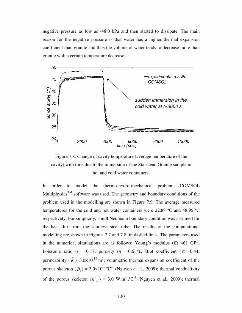
130

negative pressure as low as -48.0 kPa and then started to dissipate. The main

reason for the negative pressure is that water has a higher thermal expansion

coefficient than granite and thus the volume of water tends to decrease more than

granite with a certain temperature decrease.

Figure 7.8: Change of cavity temperature (average temperature of the

cavity) with time due to the immersion of the Stanstead Granite sample in

hot and cold water containers.

In order to model the thermo-hydro-mechanical problem, COMSOL

MultiphysicsTM software was used. The geometry and boundary conditions of the

problem used in the modelling are shown in Figure 7.9. The average measured

temperatures for the cold and hot water containers were 22.88 ºC and 48.95 ºC

respectively. For simplicity, a null Neumann boundary condition was assumed for

the heat flux from the stainless steel tube. The results of the computational

modelling are shown in Figures 7.7 and 7.8, in dashed lines. The parameters used

in the numerical simulations are as follows: Young’s modulus (E) =61 GPa,

Poisson’s ratio (ν) =0.17; porosity (n) =0.6 %; Biot coefficient (α )=0.44;

permeability ( K% )=3.0×10-18 m2; volumetric thermal expansion coefficient of the

porous skeleton ( sβ ) = 3.0×10-5 ºC-1 (Nguyen et al., 2009); thermal conductivity

of the porous skeleton ( *csk ) = 3.0 W.m-1.ºC-1 (Nguyen et al., 2009); thermal

sudden immersion in the

cold water at t=3600 s

131

conductivity of the fluid ( *cfk ) = 0.58 W.m-1.ºC-1 (Holzbecher, 1998); specific

heat capacity of the solid phase ( sc ) = 790 J.kg-1.ºC-1; specific heat capacity of the

liquid phase ( fc ) = 4187 J.kg-1.ºC-1 (Holzbecher, 1998). The dynamic viscosity

( µ ), volumetric thermal expansion coefficient ( fβ ) and specific unit weight ( fρ )

of water were assumed to be temperature dependent (Holzbecher, 1998). The

parameters used for modelling the stainless steel tube are: Young’s modulus (Ess)

=200 GPa; Poisson’s ratio (νss) =0.3; volumetric thermal expansion coefficient

( ssβ )=4.9×10-5 ºC-1; thermal conductivity ( *ssk )= 16.5 W.m-1.ºC-1; specific heat

capacity ( ssc )= 480 J.kg-1.ºC-1 (McGuire, 2008).

Figure 7.9: Geometry and boundary conditions of the THM problem.

132

The results of the numerical simulation were very close to the experimental

results obtained for the fluid cavity pressure and temperatures in the Stanstead

Granite sample. Also, no hysteresis behaviour was observed during the THM

experiments and the results were repeatable.

Figure 7.10 shows the change of cavity pressure versus temperature, plotted on

the state diagram of water. It can be seen that the temperature and pressure change

in the experiment does not change the pore fluid to a vapor, since the entire cycle

of the THM experiment is in the liquid region of the phase diagram of water.

Also, the sample is kept continuously immersed in the water with no chance for

air to enter the porous medium. Hence, although the sample experiences negative

pore pressure, based on the two reasons mentioned, it can be inferred that the

sample remains saturated during the THM test cycles and therefore the thermo-

hydro-mechanical formulation presented earlier can be used to model the

experiment.

Figure 7.10: Change of cavity pressure with respect to cavity temperature

change, plotted on the phase diagram of water (The pressure in this diagram

is absolute pressure).

133

7.5. Thermo-hydro-mechanical experiment under controlled temperature

changes

In this section, the thermo-hydro-mechanical processes in a fluid-filled cavity

located in a saturated Stanstead Granite cylinder measuring 15.24 cm in diameter

and 30.48 cm in height was investigated. The sample contains a sealed central

cavity 2.54 cm in diameter and 15.24 cm in height, which is filled with water. The

outer boundary of the sample was subjected to a controlled temperature change

and the temperature and pressure changes within the central cavity were

measured.

7.5.1. The testing apparatus

A schematic view of the test facility is shown in Figure 7.11. The sample was

initially vacuum saturated for 7 days and was then placed inside the water

container with the central cavity facing down. An annular neoprene rubber gasket

with the hardness of 60A (external diameter: 15.24 cm; internal diameter: 2.54

cm; thickness: 0.16 cm) was used to develop a seal between the bottom surface of

the sample and the stainless steel plate of the container. This contact area was

sealed against leakage by applying a 1MPa sealing stress to the top of the sample

using a hydraulic jack. A 0.635 cm diameter hole at the center of the stainless

steel plate allowed access to the central cavity. The stainless steel fitting attached

to the hole was connected to a temperature compensated pressure transducer

(Model: MMG150V5K4C1T4A6S; supplier: OMEGADYNE; maximum

pressure: 1MPa; accuracy: 0.2%) to measure the pressure change in the cavity

during the experiment. A Swagelok valve was incorporated at the stainless steel

fitting to allow water inflow. Two thermocouples (type K) were placed in the top

and bottom of the cavity to record the temperatures within the cavity. Following

the procedure developed in previous research (Selvadurai, 1996b, 2002) the wires

were passed through the fittings and marine epoxy was used to ensure that the

connections were sealed. It should be noted that the fittings were thermally

insulated using a foil-backed self adhesive foam to minimize heat loss to the

ambient environment which was maintained at approximately 25 o C .

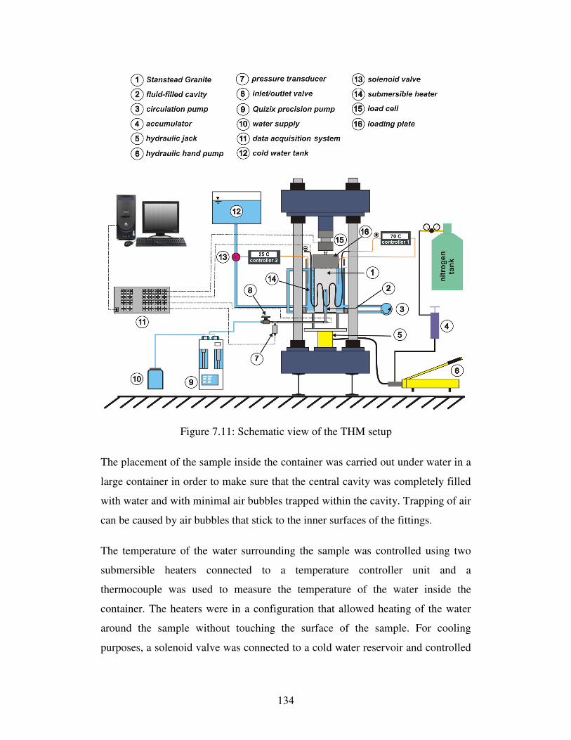
134

Figure 7.11: Schematic view of the THM setup

The placement of the sample inside the container was carried out under water in a

large container in order to make sure that the central cavity was completely filled

with water and with minimal air bubbles trapped within the cavity. Trapping of air

can be caused by air bubbles that stick to the inner surfaces of the fittings.

The temperature of the water surrounding the sample was controlled using two

submersible heaters connected to a temperature controller unit and a

thermocouple was used to measure the temperature of the water inside the

container. The heaters were in a configuration that allowed heating of the water

around the sample without touching the surface of the sample. For cooling

purposes, a solenoid valve was connected to a cold water reservoir and controlled

135

by a separate temperature controller unit and a thermocouple that measured the

temperature of the water within the container. In order to keep the temperature of

the water within the container uniform, the water was circulated using a fluid

pump. The pump constantly extracted water from the upper region of the

container and pumped it back into system at a lower section of the container.

Also, since any temperature change during the experiment can cause the sample to

shrink or expand, the sealing load that was applied by the hydraulic jack could

change. Therefore, an accumulator with an adjustable pressure release valve was

connected to the hydraulic jack in order to maintain the sealing pressure in the

correct range (1 MPa ± 0.05) during the experiment. The accumulator has a

piston connected to a Nitrogen tank with an adjustable gas pressure regulator; this

maintained the load during the cooling process and a pressure release valve

guaranteed that the expansion of the sample did not result in an increase in the

sealing load during the heating process. It should be noted that the sealing load

was measured using a load cell that was in contact with the upper platen of the

loading arrangement.

The temperature change at both the cylindrical and top surface of the sample was

measured using six thermocouples: three thermocouples measured the

temperatures at the upper, mid-height and lower levels on the boundary of the

sample and three thermocouples measured the temperature on the upper surface of

the sample (one in the center, one 2.54 cm away from the center and the third 5.08

cm away from the center). These measurements were used as temperature

boundary conditions in the numerical modelling. The outer surface of the water

container was dealt with thermal insulation (moisture-resistant Polystyrene foam

insulation, heat flow rate of 0.26 at 24 o C ) in order to minimize heat loss through

the Plexiglas and hence expedite the temperature increase inside the container.

7.5.2. Permeability measurement

Prior to performing the THM experiment, the permeability of the sample was

measured using a steady state isothermal test. Three steady state tests were

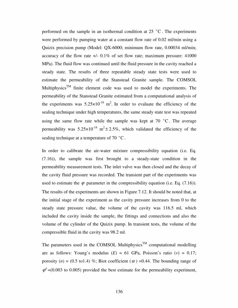
136

performed on the sample in an isothermal condition at 25 o C . The experiments

were performed by pumping water at a constant flow rate of 0.02 ml/min using a

Quizix precision pump (Model: QX-6000; minimum flow rate, 0.00034 ml/min;

accuracy of the flow rate +/- 0.1% of set flow rate; maximum pressure: 41000

MPa). The fluid flow was continued until the fluid pressure in the cavity reached a

steady state. The results of three repeatable steady state tests were used to

estimate the permeability of the Stanstead Granite sample. The COMSOL

MultiphysicsTM finite element code was used to model the experiments. The

permeability of the Stanstead Granite estimated from a computational analysis of

the experiments was 5.25×10-18 m2. In order to evaluate the efficiency of the

sealing technique under high temperatures, the same steady state test was repeated

using the same flow rate while the sample was kept at 70 o C . The average

permeability was 5.25×10-18 m2 ± 2.5%, which validated the efficiency of the

sealing technique at a temperature of 70 o C .

In order to calibrate the air-water mixture compressibility equation (i.e. Eq.

(7.16)), the sample was first brought to a steady-state condition in the

permeability measurement tests. The inlet valve was then closed and the decay of

the cavity fluid pressure was recorded. The transient part of the experiments was

used to estimate the ϕ parameter in the compressibility equation (i.e. Eq. (7.16)).

The results of the experiments are shown in Figure 7.12. It should be noted that, at

the initial stage of the experiment as the cavity pressure increases from 0 to the

steady state pressure value, the volume of the cavity was 116.5 ml, which

included the cavity inside the sample, the fittings and connections and also the

volume of the cylinder of the Quizix pump. In transient tests, the volume of the

compressible fluid in the cavity was 98.2 ml.

The parameters used in the COMSOL MultiphysicsTM computational modelling

are as follows: Young’s modulus (E) = 61 GPa, Poisson’s ratio (ν) = 0.17;

porosity (n) = (0.5 to1.4) %; Biot coefficient (α ) =0.44. The bounding range of

0ϕ =(0.003 to 0.005) provided the best estimate for the permeability experiment,

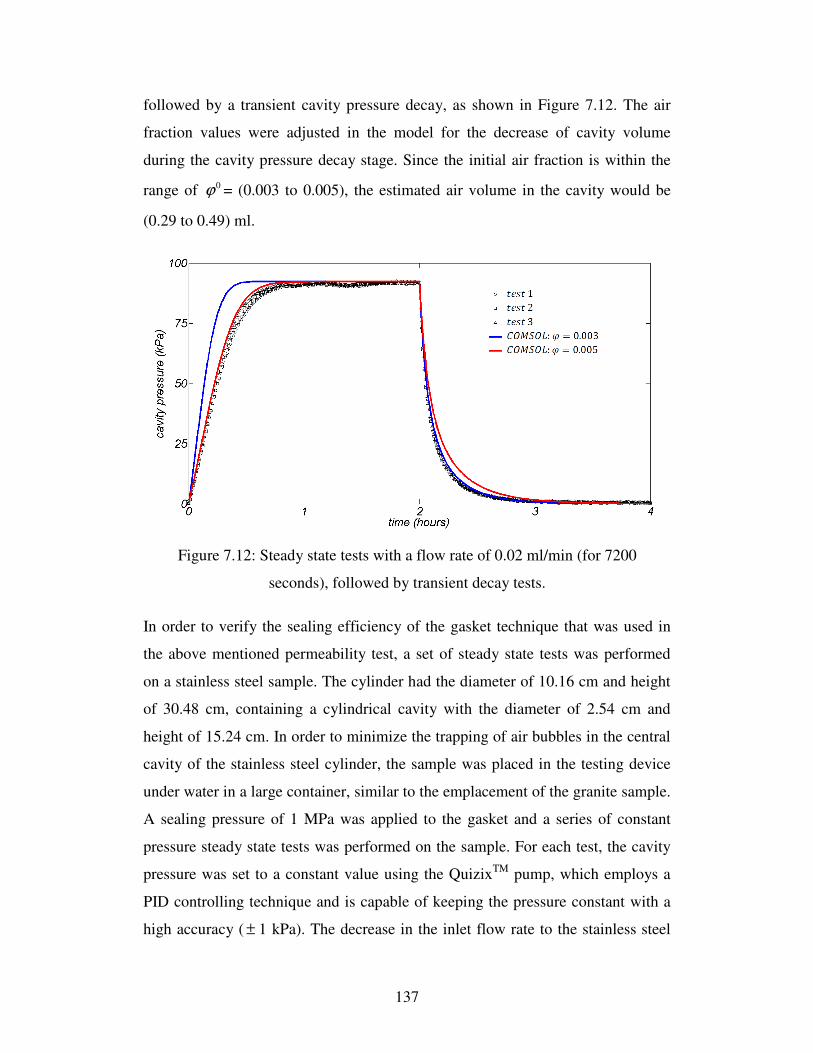
137

followed by a transient cavity pressure decay, as shown in Figure 7.12. The air

fraction values were adjusted in the model for the decrease of cavity volume

during the cavity pressure decay stage. Since the initial air fraction is within the

range of 0ϕ = (0.003 to 0.005), the estimated air volume in the cavity would be

(0.29 to 0.49) ml.


seconds), followed by transient decay tests.

In order to verify the sealing efficiency of the gasket technique that was used in

the above mentioned permeability test, a set of steady state tests was performed

on a stainless steel sample. The cylinder had the diameter of 10.16 cm and height

of 30.48 cm, containing a cylindrical cavity with the diameter of 2.54 cm and

height of 15.24 cm. In order to minimize the trapping of air bubbles in the central

cavity of the stainless steel cylinder, the sample was placed in the testing device

under water in a large container, similar to the emplacement of the granite sample.

A sealing pressure of 1 MPa was applied to the gasket and a series of constant

pressure steady state tests was performed on the sample. For each test, the cavity

pressure was set to a constant value using the QuizixTM pump, which employs a

PID controlling technique and is capable of keeping the pressure constant with a

high accuracy ( ± 1 kPa). The decrease in the inlet flow rate to the stainless steel

138

sample was monitored until it reached steady state condition. Table 7.2 shows the

results of these experiments. It was observed that the leakage through the system

was dependent on the cavity pressure; as expected, a higher cavity pressure

corresponded to a larger amount of leakage. The maximum leakage that was

measured for the 200 kPa constant pressure test was 0.000769 ml/min.

Table 7.2: The results of sealing tests performed on a stainless steel

cylinder.

P (kPa) Q (ml/min) T (Co )

200 0.000769 21.49

100 0.000240 21.16

50 8.00×10-5 21.50

25 2.00×10-5 21.50

Since the 0.02 ml/min steady state flow rate on the granite sample corresponded

to 91 kPa cavity pressure, a leakage of 0.000769 ml/min corresponds to a cavity

pressure change of 3.5 kPa. The value for the cavity pressure of 100 kPa is 1.1

kPa, which is the maximum cavity pressure achieved in the current THM test on

the granite sample. Since the diameter of the stainless steel cylinder is 33%

shorter than the Stanstead sample the estimated leakage is an upper bound for the

leakage in granite sample tested, and thus the leakage through the system

definitely can be neglected.

7.5.3. Thermo-hydro-mechanical experiment

Three heating-cooling cycles were performed on the sample by changing the

temperature of the water within the container. A general view of the THM test

configuration is shown in Figure 7.13. The temperature was initially increased

from 25 o C (laboratory temperature) to 70 o C and kept constant. The heating

process, including the initial temperature increase step and maintaining a constant

temperature, took 4 hours. The temperature at the surface of the cylinder was then

139

reduced from 70 o C to 25 o C and kept constant by circulating water at 20 o C into

the container. The cooling process took 8 hours.

Figure 7.13: The apparatus prepared for performing the THM experiment.

This heating-cooling cycle was repeated three times and the temperature and

pressure within the cavity were recorded. Each new cycle commenced after

sufficient time was allowed for complete dissipation of both temperature and

pressure. Preliminary computational estimates suggest that both the pressure and

temperature within the granite reduced to steady values at approximately 12

hours. The change in temperature at the circumference and at the upper surface of

the sample obtained for the three cycles are shown in Figures 7.14 and 7.15.

These results were used as the temperature boundary conditions in the

computational modelling.

140

Figure 7.14: The measured temperature on the circumference of the sample

during three experiments.

Figure 7.15: The measured change of temperature on the top surface of the

sample during three experiments.

7.5.4. Experimental results and computational modelling

The cavity temperature and cavity pressure measured from the three heating-

cooling cycles performed on the Stanstead Granite sample are shown,

respectively, in Figures 7.16 and 7.17. The trend in the change in cavity

temperature is very similar to the boundary temperature change. However, there is

an average time lag of 130 seconds between the start of the temperature change on

141

the surface of the sample and that in the central cavity, resulting from the heat

conduction process.

Figure 7.16: The change in the cavity temperature during the three cycles of

heating and cooling.

Figure 7.17: Comparison of the results of THM experiments with

computational results using pressure dependent compressibility values for

the cavity fluid.

142

The cavity pressure initially increased due to thermal expansion of the fluid inside

the cavity and due to the temperature-induced fluid flow from the porous medium

towards the cavity. Note that the thermal expansion of the cavity fluid is more

than the thermal expansion of the cavity itself. The pressure in the cavity reached

a maximum value of 81 kPa and then started to decay due to the dissipation of

excess pore pressure through the porous medium.

It can be seen that after 4 hours (14400 seconds) the cavity pressure reduced to

zero. At this point the cooling cycle was started and the cavity pressure became

negative. The minimum cavity pressure was recorded at -61 kPa. The negative

pressure then started to decay over the next 8 hours (28800 seconds).

With respect to the rate of heating and cooling, the cooling rate in the linear range

was 1.8 times faster than the heating rate. However, the maximum cavity pressure

during heating was higher than the maximum cavity pressure during cooling. This

is due to the fact that, although the cavities and fittings were filled with water,

there were still air bubbles trapped in the fluid inclusion which caused the

compressibility of air to be pressure dependent. Based on Eq. (7.16), the

compressibility of the air-water mixture is higher under negative pressure than

positive pressure. Thus, the cavity pressure increase is greater during heating than

in the cooling phase of the test.

The geometry and boundary conditions of the problem used in the computational

modelling are shown in Figure 7.18. The upper surface and the circumference of

the sample had a zero fluid pressure boundary conditions. The bottom surface,

which was sealed by a rubber gasket, was modelled as a no-flow boundary

condition. The temperature boundary condition for the circumference and top

surface of the sample was the temperature measured for these two surfaces; T1(t)

and T2(t) are, respectively, the average temperature values measured for the three

points at the top, mid-height and bottom of the circumference and at the center,

mid-radius and the edge of the top surface of the sample.

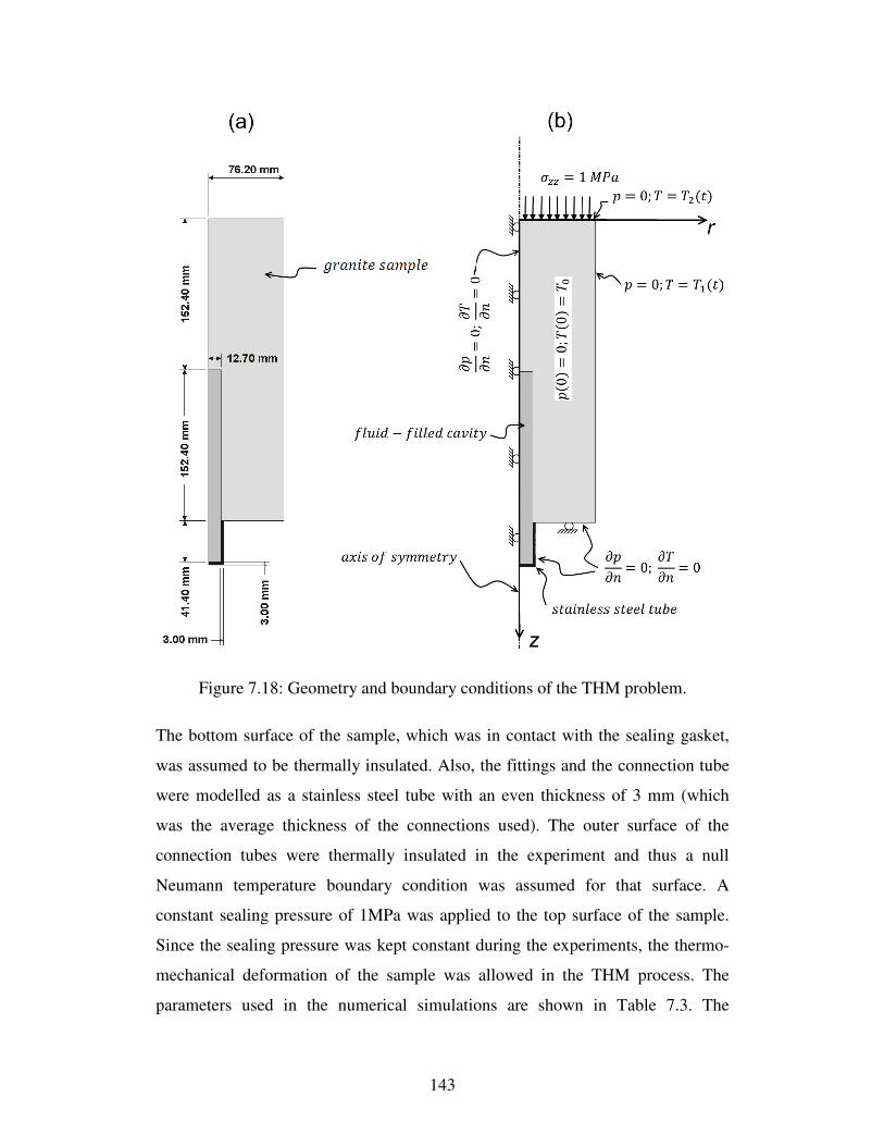
143

Figure 7.18: Geometry and boundary conditions of the THM problem.

The bottom surface of the sample, which was in contact with the sealing gasket,

was assumed to be thermally insulated. Also, the fittings and the connection tube

were modelled as a stainless steel tube with an even thickness of 3 mm (which

was the average thickness of the connections used). The outer surface of the

connection tubes were thermally insulated in the experiment and thus a null

Neumann temperature boundary condition was assumed for that surface. A

constant sealing pressure of 1MPa was applied to the top surface of the sample.

Since the sealing pressure was kept constant during the experiments, the thermo-

mechanical deformation of the sample was allowed in the THM process. The

parameters used in the numerical simulations are shown in Table 7.3. The

144

dynamic viscosity ( ( )Tµ ), volumetric thermal expansion coefficient ( ( )f Tβ ) and

specific unit weight ( ( )f Tρ ) of water were assumed to be temperature dependent

(Holzbecher, 1998).

The estimated temperature changes on the top and the bottom of the cavity are

shown in Figure 7.16. The experimental and computational results are in

agreement with each other for the temperature in the top of the cavity. However,

there is a slight discrepancy in the estimated temperature value at the bottom of

the cavity compared to the measured value. The temperature difference at the end

of the heating process is 2.45 o C . The reason for the discrepancy could be the

fact that the bottom surface of the sample, which is in contact with the rubber

gasket, was assumed to be thermally insulated in the computations. However,

based on the experimental results obtained, there is a slight heat loss through this

surface.

Table 7.3: Values of the parameters in the computational modelling of the

THM experiment.

Parameter Granite Water Stainless

Steel

Young's modulus (GPa) 61 - 200 b

Poisson's ratio 0.17 0.49 0.3 b

Porosity (%) 0. 6 100 -

Biot Coefficient 0.44 - -

permeability (m2) 5.25×10-18 (5.25×10-18) ×106 -

volumetric thermal expansion

coefficient (ºC-1) 3.0×10-5 c ( )f Tβ a 4.9×10-5 b

thermal conductivity (W.m-1.ºC-1) 3.0 c 0.58 a 16.5 b

specific heat capacity (J.kg-1.ºC-1) 790 c 4187 a 480 b a. Holzbecher (1998) b. McGuire (2008) c. Nguyen et al. (2009)

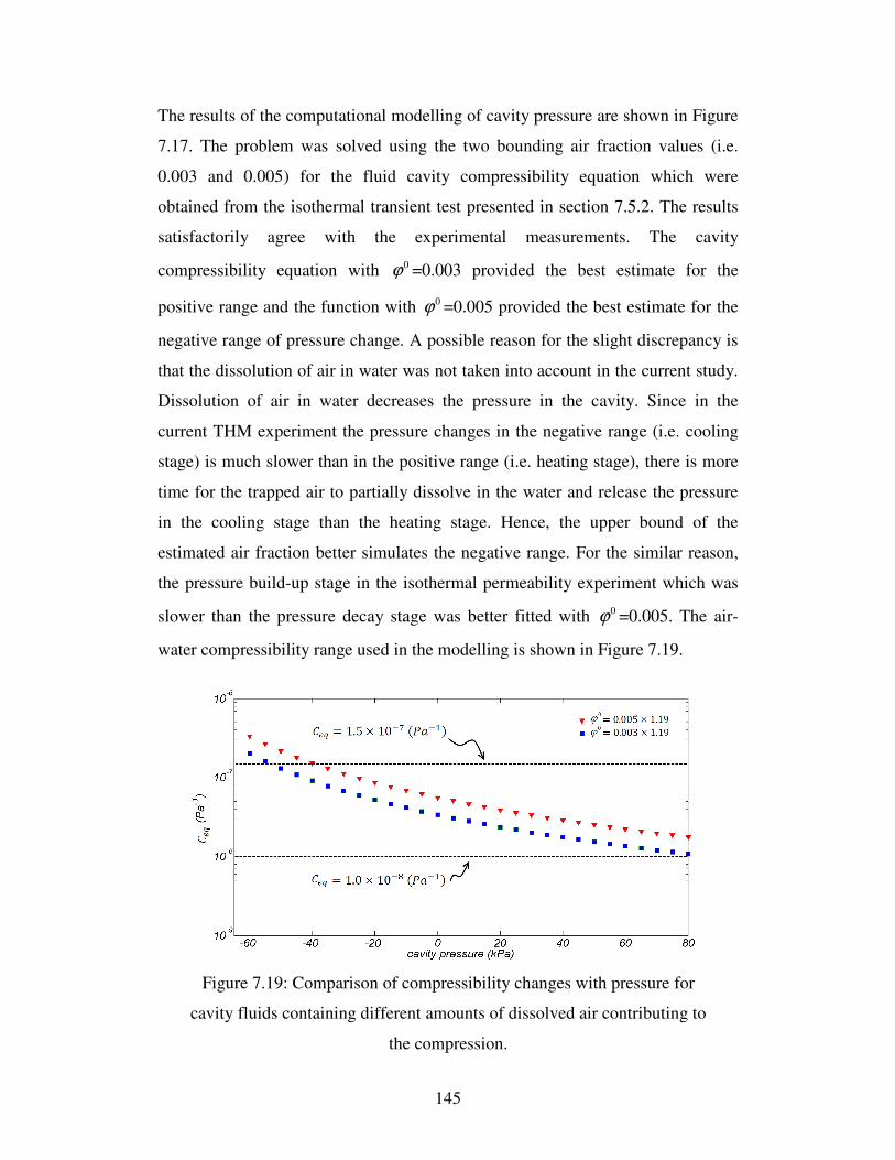
145

The results of the computational modelling of cavity pressure are shown in Figure

7.17. The problem was solved using the two bounding air fraction values (i.e.

0.003 and 0.005) for the fluid cavity compressibility equation which were

obtained from the isothermal transient test presented in section 7.5.2. The results

satisfactorily agree with the experimental measurements. The cavity

compressibility equation with 0ϕ =0.003 provided the best estimate for the

positive range and the function with 0ϕ =0.005 provided the best estimate for the

negative range of pressure change. A possible reason for the slight discrepancy is

that the dissolution of air in water was not taken into account in the current study.

Dissolution of air in water decreases the pressure in the cavity. Since in the

current THM experiment the pressure changes in the negative range (i.e. cooling

stage) is much slower than in the positive range (i.e. heating stage), there is more

time for the trapped air to partially dissolve in the water and release the pressure

in the cooling stage than the heating stage. Hence, the upper bound of the

estimated air fraction better simulates the negative range. For the similar reason,

the pressure build-up stage in the isothermal permeability experiment which was

slower than the pressure decay stage was better fitted with 0ϕ =0.005. The air-

water compressibility range used in the modelling is shown in Figure 7.19.

Figure 7.19: Comparison of compressibility changes with pressure for

cavity fluids containing different amounts of dissolved air contributing to

the compression.

146

For the purpose of comparison, the experimental results were also fitted with

constant cavity fluid compressibility values. The compressibility value of

eqC =1.0×10-8 Pa-1 provides the best estimation for the positive pressure range and

the compressibility value of eqC =1.5 ×10-7 Pa-1 provides the best estimation for

the negative pressure range. The results are shown in Figure 7.20.

Figure 7.20: Comparison of the results of THM experiments with

computational results using constant compressibility values for the cavity

fluid.

Another observation is that the cavity pressure changes at the early stages of

heating and cooling, when the temperature change has not yet affected the cavity

fluid. These effects are shown in Figures 7.21 and 7.22. Immediately after the

start of the heating stage, the cavity pressure begins to decrease, reaching – 1 kPa

and then reducing to zero pressure after 500 seconds. Similarly, at the very early

stage of cooling, the cavity pressure increases from 2.7 kPa and reaches a

maximum pressure of 6.5 kPa; it then decreases and returns to 2.7 kPa after

almost 500 seconds. This phenomenon is due to the fact that the very early

temperature change on the surface of the sample causes the surface region of the

sample to expand or shrink in heating and cooling, respectively. This is the

147

Mandel-Cryer effect associated with temperature change (Kodashima and

Kurashige, 1996; Selvadurai and Suvorov, 2012).

Figure 7.21: Volumetric expansion of the cavity due to a temperature

increase on the sample surface at the start of the heating stage ( 0ϕ =0.005).

In order to study the possibility of de-saturation during the heating-cooling cycles,

the change in the maximum absolute pressure versus temperature for the cavity

was plotted on the state diagram of water (see Figure 7.23). Since the whole cycle

of pressure-temperature change in the experiment is in the liquid state, it can be

inferred that there is no possibility of de-saturation of the sample during the

experiment and therefore the saturated THM formulation is applicable for

modelling purposes.

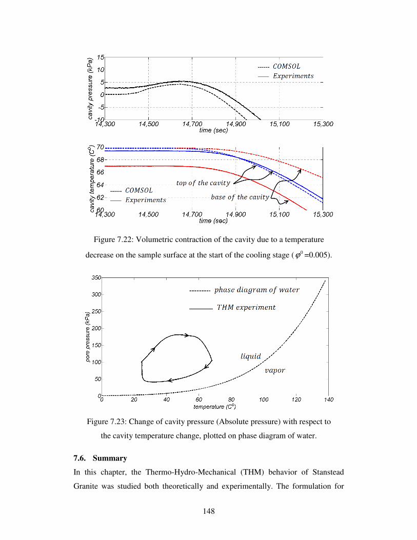
148

Figure 7.22: Volumetric contraction of the cavity due to a temperature

decrease on the sample surface at the start of the cooling stage ( 0ϕ =0.005).

Figure 7.23: Change of cavity pressure (Absolute pressure) with respect to

the cavity temperature change, plotted on phase diagram of water.

7.6. Summary

In this chapter, the Thermo-Hydro-Mechanical (THM) behavior of Stanstead

Granite was studied both theoretically and experimentally. The formulation for

149

non-isothermal poroelasticity in saturated geomaterials was summarized and two

experimental investigations were performed to verify the accuracy of the THM

formula. The experiments were conducted to examine the THM processes that can

be generated in a granite cylinder with permeability in the range (3 to 6) ×10-18

m2. A fluid-filled cavity within a Stanstead Granite cylinder is used to examine

the process of pressure generation during heating of the outer surface. The first

experiment was performed on a Stanstead Granite cylinder measuring roughly 5

cm in diameter and 10 cm in height. The sample was subjected to cycles of

heating and cooling at the boundary by immersion in hot and cold reservoirs and

the experiments were repeated 6 times. The second experiment was performed on

a larger Stanstead Granite cylinder measuring 15 in diameter and 30 cm in height.

The temperature was increased and decreased as a ramp function, using PID

temperature controllers. The heating-cooling cycles were repeated 3 times. The

experimental results for each experiment were evaluated within the content of a

THM model that takes into account heat conduction in the saturated granite and

Darcy flow-based classical poroelasticity. Nominal calculations were also

performed to account for (i) temperature dependency of the density and fluid

viscosity and (ii) alteration in the compressibility of the pore fluid in the system

due to the presence of any air. The result of the experiments indicates that

pressure changes can be modelled accurately using the finite element software

COMSOLTM that can examine THM processes. The factor that contributes to the

slight discrepancy between experimental and computational results is identified as

possible air entrainment (through parametric computational evaluation), which

also accounts for the pressure-dependent compressibility. The experimentation

can be further improved by adapting the procedures to eliminate the influences of

air content, both free and dissolved, on the THM processes. Such refinements are

considered to be much too artificial since in practice, where the theories are used

to estimate the THM behavior of rocks in situ, there are no assurances of complete

saturation. The research work indicates that conventional THM models can be

used to model the heating behavior of granite relatively accurately. The

150

development of pressure within a fluid-filled cavity is the candidate problem

examined to validate the modelling.

151

CHAPTER 8

CONCLUSIONS AND SCOPE FOR FUTURE RESEARCH

8.1. Summary and concluding remarks

Biot’s theory of linear poroelasticity can be extended to include thermal effects.

The study of the thermo-hydro-mechanical (THM) behaviour of porous media is

of interest in several disciplines of engineering; the major areas of application in

geotechnical engineering are deep disposal of nuclear wastes in geological

repositories, oil and gas recovery, geothermal energy, and CO2 sequestration. The

focus of this thesis has been on the non-isothermal transport of fluid in Stanstead

Granite, which is a low permeability geomaterial similar to those being

considered as candidate rocks for the deep geological disposal of nuclear wastes.

The THM behaviour of the rock was studied both theoretically and

experimentally. The following is a summary of the research performed on the

interpretation of non-isothermal transport in Stanstead Granite:

• The physical and mechanical characterization of Stanstead Granite was

performed through a series of laboratory experiments. The chemical

composition of the rock was studied through X-ray fluorescence spectrometry

152

tests performed on the material in the Earth and Planetary Science

Department of McGill University. The two major elements identified were

silicon (70%) and aluminum (15%), which is similar to other granitic rocks.

The porosity of the rock was measured using both a saturation technique and

mercury intrusion porosimetry (MIP). The porosity was measured to be

(0.4% to 0.7%) from the saturation technique and (0.7% to 1.4%) using MIP.

Since the MIP technique measures the total area of the pores on the surface,

including the non-connected pores, the result is an upper bound for the

porosity. The bulk dry density and the grain density of the rock were

measured as (2630 kg/m3 to 2660 kg/m3) and (2650 kg/m3 to 2670 kg/m3)

respectively. Also, 4 unconfined compressive strength (UCS) tests were

performed on cylindrical samples of Stanstead Granite that measured 5 cm in

diameter and 10 cm in height; the rocks showed linear elastic behaviour and

failed at an average uniaxial compressive stress of 132 MPa. The average

Young’s modulus was measured at 61 GPa and the Poisson’s ratio was 0.17.

The physical and mechanical parameters measured compare favourably with

similar results for intact granitic rocks reported in the literature.

• The isothermal transport of fluid through porous media was theoretically

studied (Chapter 3). Terzaghi’s theory of one-dimensional consolidation was

presented along with its three-dimensional extension. The theory weakly

takes into account the effect of skeletal deformation on the transient flow of

fluid induced by the application of traction on the surface of a one-

dimensional column of soil. Biot’s theory of linear poroelasticity was also

presented. This formulation takes into account the coupling effects between

the pore pressure and skeletal deformation. It also assumes that the solid

skeleton, the permeating fluid, and the solid grains are compressible; the

latter two are assumed to be incompressible in Terzaghi’s consolidation

theory. In the limiting case where the pore pressure uncouples from the stress

field, the fluid phase equation in Biot’s formulation reduces to the piezo-

conduction equation, which has only the pore pressure as a variable.

153

• For low permeability geomaterials, the preferred method for measuring

permeability is through hydraulic pulse testing. An analysis of the

experimental results can be performed by the application of either Biot’s

theory of linear poroelasticity or the piezo-conduction equation. The accuracy

of using the piezo-conduction equation to estimate the permeability was

studied using published data on the material properties of two different rocks

types: Westerly Granite, and Indiana Limestone. It was seen that the

application of the commonly used piezo-conduction equation, which neglects

the compressibility of solid grains, results in a noticeable overestimation of

permeability. However, the use of the piezo-conduction equation with a

specific storage term that takes into account the effect of compressibility of

solid grains, gives a negligible error. Also it was seen that the above

mentioned modelling error is highest for the one-dimensional test, and is

lower for the radial flow and patch pulse tests, respectively.

• A series of steady state tests was performed on 7 different samples of

Stanstead Granite. The tests were performed on partially drilled and undrilled

cylindrical samples with dimensions varying from the smallest with a

diameter of D =5 cm and a length of L =10 cm to the largest with D =15 cm

and L =30 cm. The tests on the samples with the partially drilled cavity

provided both radial and axial flow patterns; however, for the geometries of

the tested samples, the shortest path from the central cavity to the outer

surface of the samples was radial (i.e. the dominant flow pattern was radial).

The permeability was in the range of (3 to 6)×10-18 m2 for unstressed

samples. The one-dimensional flow tests were performed under isotropic

stress in a triaxial cell. For the samples tested under an isotropic stress of 5

MPa, the permeability was within the range of (1 to 2)×10-18 m2.

• A series of hydraulic pulse tests were also performed on 4 different samples

of Stanstead Granite. The tests included radially-symmetric flow, patch pulse

tests and tests on partially drilled samples. It was seen that, no matter how

precise the attempts to fill the cavity with de-aired water were, air bubbles

154

still remain in the system. This can significantly affect the compressibility of

water and the permeability estimates from the hydraulic pulse tests can be

orders of magnitude lower than in reality; therefore, the compressibility has

to be corrected for unwanted air entrained as air bubbles in the cavity. The

air-water mixture compressibility was discussed and a relationship was

presented. Following the proposed algorithm for estimating the amount of

trapped air bubbles in the fluid cavity, the permeability of the tested Stanstead

Granite samples was estimated to be (3 to 6)×10-18 m2.

• The alteration in the permeability of Stanstead Granite under isotropic

loading and unloading was experimentally studied, using a steady state

permeability measurement technique. Rock specimens in the lab are under

zero stresses whereas an in-situ rock mass is subject to geostatic stresses. Any

change in the confining stress can alter the permeability of geomaterials. A

series of constant flow rate steady state tests was performed on 3 cylindrical

samples of Stanstead Granite, under various confining pressures. The tests

were performed in a GDS triaxial cell. It was seen that when the confining

pressure is increased to 30 MPa the permeability decreased by almost one

order of magnitude and, after unloading, it returned to its preloaded value.

Loading the samples up to 60 MPa decreased the permeability between (2 to

3) orders of magnitude. When the samples were unloaded, although the

permeability increased, it did not return to its original value. This temporary

decrease in permeability under isotropic loading can be associated with the

elastic closure of pores and micro-cracks, whereas the permanent decrease

can be due to pore collapse. In order to study the hydraulic anisotropy in the

rock, one sample was cored, with its central axis perpendicular to that in the

other two samples. The Stanstead Granite samples tested showed isotropy in

permeability up to the confining pressure of 40 MPa. However, a further

increase of confining pressure to 60 MPa showed that anisotropy developed

with the ratio of 1:3. This ratio was retained during unloading.

155

• The thermo-hydro-mechanical behaviour of Stanstead Granite was also

studied. The non-isothermal extension of Biot’s theory of linear poroelasticity

was presented. Since the measurement of fluid pressure and temperature in

the sealed cavity is experimentally feasible, this was implemented in the

research. Nominal calculations were also performed to account for

temperature dependency in the density and viscosity of the fluid; alteration in

the compressibility of the pore fluid in the system due to any presence of air

was also accounted for. A thermal damage test was performed on a

cylindrical sample measuring 15 cm in diameter and 30 cm in height. It was

observed that after an abrupt temperature increase of 80 Co the permeability

increased between 25% to 40%. Two different THM experiments were

performed and the results were used to investigate the accuracy of the

presented THM formulation. In the first experiment, a sample was heated by

immersion in a hot water bath and cooled by immersion in a cold water bath.

For the second THM experiment, a unique apparatus was designed and

fabricated; this test facility is capable of changing the temperature in a

controlled fashion. The sealing of the system was verified by performing tests

on a stainless steel cylinder, with the result that a sealing load could be kept

constant during the temperature variations. In both of the experiments, the

change of temperature and pressure in the sealed fluid cavity was monitored.

The problems were computationally modelled using the presented

formulation. The COMSOL MultiphysicsTM finite element code was used to

solve the governing partial differential equations. The results obtained in the

simulations compared favourably with the measured temperature and pore

pressure values. The slight discrepancy was associated with the existence of

air bubbles in the fluid-filled cavity.

8.2. Scope for future research

In the current research, the isothermal and non-isothermal fluid transport in

Stanstead Granite was studied, both theoretically and experimentally. The

following investigations can be suggested as future work:

156

• In this research, fluid flow was studied only in saturated geomaterials,

whereas in many practical situations the medium is unsaturated. Any future

research can extend the theoretical and experimental work to the study of the

unsaturated thermo-hydro-mechanical behaviour of low permeability

geomaterials.

• The alteration in the permeability of Stanstead Granite due to isotropic

loading and unloading was studied; it was observed that, after a certain level

of confining pressure, the pore closure and subsequent permeability decrease

becomes partially irreversible. Further investigations can be performed by

comparing CT-scanned images of a rock sample before and after an isotropic

load. A further approach would be to perform the same comparison between

the results of mercury intrusion porosimetry tests before and after an isotropic

load.

• The compressibility of the air-water mixture was studied and an algorithm

was proposed to correct for the effect of air entrainment in the sealed cavity

used in hydraulic pulse testing. It was mentioned that the air bubbles can go

into solution, according to Henry’s Law and the rate of dissolution follows

Fick’s Law. However, the transient process of dissolution of air into water

was neglected. Further investigations could be conducted to take this effect

into account.

• Any thermal, hydrological, or mechanical process can induce damage to the

fabric of a porous medium. In the current research, the range of the thermo-

hydro-mechanical loads was restricted to values that do not alter the

characteristics of the rock and therefore no damage was observed in the

experiments. An extension of this research could be the study of the THM

behaviour of damage-susceptible geomaterials.

• The samples used in the THM tests were cylinders with partially drilled

central cavities, heated on the outer boundaries. Performing tests on samples

with different geometries and boundary conditions, along with strain gauge

157

instrumentation of the samples, could provide more information on the

coupling behaviour of low permeability rocks under thermal loads.

158

REFERENCES

Aboustit, B.L., Advani, S.H. & Lee, J.K. (1985), Variational principles and finite

element simulations for thermo‐elastic consolidation. International Journal for

Numerical and Analytical Methods in Geomechanics, Vol. 9, 49-69.

Adachi, J. & Detournay, E. (1997), A Poroelastic solution of the oscillating pore

pressure method to measure permeabilities of ''tight'' rocks. International

Journal of Rock Mechanics and Mining Sciences and Geomechanics Abstracts,

1997; 430.

Aligizaki, K.K. (2006), Pore Structure of Cement-based Materials: Testing,

Interpretation and Requirements, Taylor & Francis, New York.

Alonso, E.E., Alcoverro, J., Coste, F., Malinsky, L., Merrien-Soukatchoff, V.,

Kadiri, I., Nowak, T., Shao, H., Nguyen, T.S., Selvadurai, A.P.S., Armand, G.,

Sobolik, S.R., Itamura, M., Stone, C.M., Webb, S.W., Rajeb, A., Tijani, M.,

Maouche, Z., Kobayashi, A., Huikami, H., Ito, A., Sugita, Y,. Chijimatsu, M.,

Borgesson, L., Hernelind, J., Rutqvist, J., Tsang, C.F. & Jussia, P. (2005), The

FEBEX benchmark test: case definition and comparison of modelling

approaches. International Journal of Rock Mechanics and Mining Sciences,

Vol. 42, 611-638.

ASTM D2936-08 (2004), Standard test method for direct tensile strength of intact

rock core specimens.

ASTM D3967-08 (2004), Standard test method for splitting tensile strength of

intact rock core specimens.

ASTM D4404-84 (2004), Standard test method for determination of pore volume

and pore volume distribution of soil and rock by mercury intrusion

porosimetry.

159

ASTM D7012-04 (2004), Standard test method for compressive strength and

elastic moduli of intact rock core specimens under varying states of stress and

temperature.

Bachu, S. (2008), CO2 storage in geological media: role, means, status and

barriers to deployment. Progress in Energy and Combustion Sciences, Vol. 34,

254-273.

Bai, M & Roegiers, J.C. (1994), Fluid flow and heat flow in deformable fractured

porous media. International Journal of Engineering Science, Vol. 32, 1615-

1633.

Barenblatt, G.I., Entov, V.M. & Ryzhik, V.M. (1989), Theory of Fluid Flows

through Natural Rocks. Kluwer Academic Publishers, Boston.

Barron, R.A. (1948), The influence of drain wells on the consolidation of fine-

grained soils. Transact ASCE, Vol. 113, 718-742.

Bear, J. (1972), Dynamics of Fluids in Porous Media. Dover Publications, New

York.

Belotserkovets, A. & Prevost, J.H. (2011), Thermoporoelastic response of a fluid-

saturated porous sphere: An analytical solution. International Journal of

Engineering Science, Vol. 49, 1415-1423.

Berge, P.A., Wang, H.F. & Bonner, B.P. (1993), Pore pressure buildup coefficient

in synthetic and natural sandstones. International Journal of Rock Mechanics

and Mining Sciences and Geomechanics Abstracts, Vol. 30, 1135-1141.

Bernabe, Y. (1986), The effective pressure law for permeability in Chelmsford

Granite and Barre Granite. International Journal of Rock Mechanics and

Mining Science, Vol. 23, 267-275.

Biot, M.A. (1941a), General theory of three‐dimensional consolidation. Journal of

Applied Physics, Vol. 12, 155-164.

Biot, M.A. (1941b), Consolidation settlement under a rectangular load

distribution. Journal of Applied Physics, Vol. 12, 426-430.

160

Biot, M.A. (1955), Theory of elasticity and consolidation for a porous anisotropic

solid. Journal of Applied Physics, Vol. 26, 182-185.

Biot, M.A. (1956), General solutions of the equations of elasticity and

consolidation for a porous material. Journal of applied Mechanics, Vol. 23, 91-

96.

Biot, M.A. & Clingan, F.M. (1941), Consolidation settlement of a soil with an

impervious top surface. Journal of Applied Physics, Vol. 12, 578-581.

Biot, M.A. & Clingan, F.M. (1942), Bending settlement of a slab resting on a

consolidating foundation. Journal of Applied Physics, Vol. 13, 35-40.

Biot, M.A. & Willis, D.G. (1957) The elastic coefficients of the theory of

consolidation. Journal of Applied Mechanics, Vol. 24, 594-601.

Blatt, H., Tracy, R. & Owens, B. (2005), Petrology: Igneous, Sedimentary, and

Metamorphic, WH Freeman, New York.

Booker, J.R. & Savvidou, C. (1984), Consolidation around a spherical heat

source. International Journal of Solids and Structures, Vol. 20, 1079-1090.

Booker, J.R. & Savvidou, C. (1985), Consolidation around a point heat source.

International Journal for Numerical and Analytical Methods in Geomechanics,

Vol. 9, 173-184.

Boone, T.J. & Detournay, E. (1990), Response of a vertical hydraulic fracture

intersecting a poroelastic formation bounded by semi-infinite impermeable

elastic layer. International Journal of Rock Mechanics and Mining Sciences

and Geomechanics Abstracts, Vol. 27, 189-197.

Bowen, R.M. (1980), Incompressible porous media models by use of the theory of

mixtures. International Journal of Engineering Science, Vol. 18, 1129-1148.

Brace, W.F., Walsh, J.B. & Frangos, W.T. (1968), Permeability of granite under

high pressure. Journal of Geophysical Research, Vol. 73, 2225-2236.

161

Bredehoeft, J.D. & Papadopulos, S.S. (1980), A method for determining the

hydraulic properties of tight formations. Water Resources Research, Vol. 16,

233-238.

Brownell, Jr D.H., Garg, S.K. & Pritchett, J.W. (1977), Governing equations for

geothermal reservoirs. Water Resources Research, Vol. 13, 929-934.

Bodvarsson, G.S. & Stefansson, V. (1989), Some theoretical and field aspects of

reinjection in geothermal reservoirs. Water Resources Research, Vol. 25, 1235-

1248.

Burbey, T. (2008), The influence of geologic structure on deformation due to

ground water withdrawal. Ground Water, Vol. 46, 202-211.

Carmichael, R.S. (1982), Handbook of Physical Properties of Rocks, CRC Press,

Florida.

Carnaffan, P. (1994), An experimental technique for determining the permeability

of rock, concrete and cement grout, M.Eng. thesis, Department of Civil

Engineering and Environmental Engineering, Carlton University, Ottawa.

Carsla,w H.S. & Jaeger, J.C. (1959), Conduction of heat in solids, Oxford

University Press, London.

Chen, Y., Zhou, C. & Jing, L. (2009), Modeling coupled THM processes of

geological porous media with multiphase flow: theory and validation against

laboratory and field scale experiments. Computers and Geotechnics, Vol. 36,

1308-1329.

Chijimatsu, M., Nguyen, T.S., Jing, L., De Jonge, J., Kohlmeire, M., Millard, A.,

Rajeb, A., Rutqvist, J., Souley, M. & Sugita, Y.(2005), Numerical study of the

THM effects on the near-field safety of a hypothetical nuclear waste

repository—BMT1 of the DECOVALEX III project. Part 1: conceptualization

and characterization of the problems and summary of results. International

Journal of Rock Mechanics and Mining Sciences, Vol. 42, 720-730.

162

Cooper, Jr H.H., Bredehoeft, J.D. & Papadopulos, I.S. (1967), Response of a

finite-diameter well to an instantaneous charge of water. Water Resources

Research, Vol. 3, 263-269.

Coussy, O. (1989), A general theory of thermoporoelastoplasticity for saturated

porous materials. Transport in Porous Media, Vol. 4, 281-293.

Coussy, O. (1995), Mechanics of Porous Continua, John Wiley & Sons,

Chichester.

Cryer, C.W. (1963), A comparison of the three-dimensional consolidation theories

of Biot and Terzaghi. The Quarterly Journal of Mechanics and Applied

Mathematics, Vol. 16, 401-412.

Darcy, H. (1856), Les Fontaines Publiques de la Ville de Dijon, Dalmont, Paris.

de Boer, R. (1999), Porous Media: Theory and Experiments, Kluwer Academic,

New York.

de Boer, R. (2005), The Engineer and the Scandal: a Piece of Science History,

Springer, Berlin.

de Jong, G.J. & Verruijt, A. (1965), Primary and secondary consolidation of a

spherical clay sample. In Proceedings of the Sixth International Conference on

Soil Mechanics and Foundation Engineering. Montreal, Canada, Vol. 1, pp.

254-258. Toronto: University of Toronto Press.

de Wet, J. (1962), Highway Research Board, US Nat. Acad. Sc. Bulletin.

Dewiere, L., Plas, F. & Tsang, C.F. (1996), Lessons learned from DECOVALEX.

Developments in Geotechnical Engineering, Vol. 79, 495-504.

Detournay, E. & Cheng, A.H-D. (1990), Plane strain analysis of a stationary

hydraulic fracture in a poroelastic medium. International Journal of Solids and

Structures, Vol. 27, 1645-1662.

Detournay, E & Cheng, A.H-D. (1993), Fundamentals of poroelasticity. In

Comprehensive Rock Engineering (ed. J.A. Hudson), pp. 113-171. New York:

Pergamon Press.

163

Dewiere, L., Plas, F. & Tsang, C.F. (1996), Lessons learned from DECOVALEX.

Developments in Geotechnical Engineering, Vol. 79, 495-504.

Fillunger, P. (1936), Erdbaumechanik?, Selbstverl, Vienna.

Fredlund, D.G. (1976), Density and compressibility characteristics of air-water

mixtures. Canadian Geotechnical Journal, Vol. 13, 386-396.

Geertsma, J. (1973), Land subsidence above compacting oil and gas reservoirs.

Journal of Petroleum Technology, Vol. 25, 734-744.

Gens, A., Garcia‐Molina, A.J., Olivella, S., Alonso, E.E. & Huertas, F. (1998),

Analysis of a full scale in situ test simulating repository conditions.


Vol. 22, 515-548.

Gibson, R.E., Gobert, A. & Schiffman, R.L. (1989), On Cryer's problem with

large displacements. International Journal for Numerical and Analytical

Methods in Geomechanics, Vol. 13, 251-262.

Gibson, R., Knight, K. & Taylor, P. (1963), A critical experiment to examine

theories of three-dimensional consolidation. In Proceedings of European

Conference on Soil Mechanics and Foundation Engineering, Vol. 1, pp. 69-76,

Wiesbaden: Deutsche Gesellschaft für Erd-und Grundbau.

Gorban, B.D., Brigham, W.E. & Ramey Jr, H.J. (1987), Absolute permeability as

a function of confining pressure, pore pressure, and temperature. Society of

Petroleum Engineering-Formation Evaluation, Vol. 2, 77-84.

Gurtin, M.E. (1966), Variational principles for linear initial value problems.

Quarterly of Applied Mathematics, Vol. 12, 252-256.

Gutierrez, M. & Makurat, A. (1997), Coupled THM modelling of cold water

injection in fractured hydrocarbon reservoirs. International Journal of Rock

Mechanics and Mining Science, Vol. 34, 113.e1–113.e15.

Hansbo, S. (1979), Consolidation of clay by band-shaped prefabricated drains.

Ground Engineering, Vol. 12, 16-25.

164

Hansbo, S. (1981), Consolidation of fine-grained soils by prefabricated drains. In

Proceedings of the 10th

International Conference on Soil Mechanics and

Foundation Engineering, Stockhom, (ed. Publications Committee of X.

ICSMFE), pp. 677-682. Rotterdam: Balkema

Hart, D.J. & Wang, H.F. (1995), Laboratory measurements of a complete set of

poroelastic moduli for Berea sandstone and Indiana limestone. Journal of

Geophysical Research, Vol. 100, 17741-17751.

Hart, D.J. & Wang, H.F. (1998), Poroelastic effects during a laboratory transient

pore pressure test. In Poromechanics (ed. J.F. Thimus, Y. Abousleiman, A.H.-

D. Cheng, O. Coussy & E. Detournay), pp. 579-582. Rotterdam: Balkema.

Heiland, J. (2003), Laboratory testing of coupled hydro-mechanical processes

during rock deformation. Hydrogeology Journal, Vol. 11, 122-141.

Heinrich, V.G. & Desoyer, K. (1961), Theorie dreidimensionaler

Setzungsvorgänge in Tonschichten. Archive of Applied Mechanics, Vol. 30,

225-253.

Heystee, R. & Roegiers, J.-C. (1981), The effect of stress on the primary

permeability of rock cores-a facet of hydraulic fracturing. Canadian

Geotechnical Journal, Vol. 18, 195-204.

Holzbecher, E.O. (1998), Modeling Density-Driven Flow in Porous Media:

Principles, Numerics, Software, Springer, New York.

Hsieh, P.A. (1996), Deformation-induced changes in hydraulic head during

ground-water withdrawal. Ground Water, Vo. 34, 1082-1089.

Hsieh, P.A., Tracy, J.V., Neuzil, C.E., Bredehoeft, J.D. & Silliman, S.E. (1981), A

transient laboratory method for determining the hydraulic properties of

‘tight’rocks—I. theory. International Journal of Rock Mechanics and Mining

Sciences and Geomechanics Abstracts, Vol. 18, 245-252.

Ilyasov, M., Ostermann, I. & Punzi, A. (2010), Modelling deep geothermal

reservoirs: recent advances and future problems. In Handbook of

165

Geomathematics (ed. W., Freeden, M.Z. Nashed & T., Sonar), pp. 679-711.

Berlin: Springer.

Iqbal M.J. & Mohanty, B. (2007), Experimental calibration of ISRM suggested

fracture toughness measurement techniques in selected brittle rocks. Rock

Mechanics and Rock Engineering, Vol. 40, 453-475.

Jing, L., Tsang, C.F. & Stephansson, O. (1995), DECOVALEX-an international

co-operative research project on mathematical models of coupled THM

processes for safety analysis of radioactive waste repositories. International

Journal of Rock Mechanics and Mining Sciences and Geomechanics Abstracts,

Vol. 5, 389-398.

Kiyama, T., Kita, H., Ishijima, Y., Yanagidani, T., Aoki, K. & Sato T. (1996),

Permeability in anisotropic granite under hydrostatic compression and triaxial

compression including post-failure region. In Proceedings of 2nd

North

American Rock Mechanics Symposium (ed. M. Aubertin, F. Hassani & H.

Mitri), pp. 1643-1650. Rotterdam: Taylor & Francis.

Kodashima, T. & Kurashige, M. (1996), Thermal stresses in a fluid-saturated

poroelastic hollow sphere. Journal of Thermal Stresses, Vol. 19, 139-151.

Kranz, R.L., Frankel, A.D., Engelder, T. & Scholz, C.H. (1979), The permeability

of whole and jointed Barre granite. International Journal of Rock Mechanics

and Mining Sciences and Geomechanics Abstracts, Vol. 16, 225-234.

Kranz, R.L., Saltzman, J.S. & Blacic, J.D. (1990), Hydraulic diffusivity

measurements on laboratory rock samples using an oscillating pore pressure

method. International Journal of Rock Mechanics and Mining Sciences and

Geomechanics Abstracts, Vol. 27, 345-352.

Lecampion, B., Constantinescu, A. & Malinsky, L. (2006), Identification of

poroelastic constants of “tight” rocks from laboratory tests. International

Journal of Geomechanics, Vol. 6, 201-208.

166

Lemieux, J.-M. (2011), Review: the potential impact of underground geological

storage of carbon dioxide in deep saline aquifers on shallow groundwater

resources. Hydrogeology Journal, Vol. 19, 757-778.

Lewis, R.W. & Schrefler, B.A. (1998), The Finite Element Method in the Static

and Dynamic Deformation and Consolidation of Porous Media, John Wiley,

Chichester.

Lin, W. (1977), Compressible fluid flow through rocks of variable permeability.

Lawrence Livermore Laboratory, Livermore, California, Rept. UCRL-52304.

Mandel, J. (1953), Consolidation des sols (Étude Mathématique). Geotechnique,

Vol. 3, 287-299.

Mason, D.P., Solomon, A. & Nicolaysen, L.O. (1991), Evolution of stress and

strain during the consolidation of a fluid‐saturated porous elastic sphere.

Journal of Applied Physics, Vol. 70, 4724-4740.

McGuire, M.F. (2008), Stainless Steels for Design Engineers, ASM International,

Ohio.

McNamee, J. & Gibson, R.E. (1960a), Displacement functions and linear

transforms applied to diffusion through porous elastic media. The Quarterly

Journal of Mechanics and Applied Mathematics, Vol. 13, 98-111.

McNamee, J. & Gibson, R.E. (1960b), Plane strain and axially symmetric

problems of the consolidation of a semi-infinite clay stratum. The Quarterly

Journal of Mechanics and Applied Mathematics, Vol. 13, 210-227.

McTigue, D.F. (1986), Thermoelastic response of fluid‐saturated porous rock.

Journal of Geophysical Research: Solid Earth, Vol. 91, 9533-9542.

Millard. A., Rajeb, A., Chijimatsu, M., Jing, L., De Jonge, J., Kohlmeier, M.,

Nguyen, T.S., Rutqvist, J., Souley M. & Sugita, Y. (2005), Numerical study of

the THM effects on the near-field safety of a hypothetical nuclear waste

repository—BMT1 of the DECOVALEX III project. Part 2: effects of THM

167

coupling in continuous and homogeneous rocks. International Journal of Rock

Mechanics and Mining Sciences, Vol. 42, 731-744.

Morin, R.H & Olsen, H.W. (1987), Theoretical analysis of the transient pressure

response from a constant flow rate hydraulic conductivity test. Water

Resources Research, Vol. 23, 1461-1470.

Morland, L.W. (1978), A theory of slow fluid flow through a porous

thermoelastic matrix. Geophysical Journal of the Royal Astronomical Society,

Vol. 55, 393-410.

Murayama, S. & Akai, K. (1954), Failure of the embankment foundation (Studies

on the failure and the settlement of foundations). Bulletins-Disaster Prevention

Research Institute, Kyoto University, Vol. 8, 1-15.

Nasseri, M.H.B, Grasselli, G & Mohanty, B. (2010), Fracture toughness and

fracture roughness in anisotropic granitic rocks. Rock Mechanics and Rock

Engineering, Vol. 43, 403-415.

Nakao, S, & Ishido, T. (1998), Pressure-transient behaviour during cold water

injection into geothermal wells. Geothermics, Vol. 27, 401-413.

Naylor, A.H. (1948), Precise determination of primary consolidation. In

Proceedings of the 2nd

International Conference on Soil Mechanics and

Foundation Engineering, Rotterdam, the Netherlands (ed. Publications

Committee of II. ICSMFE), pp. 34-40. Rotterdam: Balkema

Neuzil, C.E., Cooley, C., Silliman, S.E., Bredehoeft, J.D. & Hsieh, P.A. (1981), A

transient laboratory method for determining the hydraulic properties of

‘tight’rocks—II. Application. International Journal of Rock Mechanics and

Mining Sciences and Geomechanics Abstracts, Vol. 18, 253-258.

Nguyen, T.S. & Selvadurai, A.P.S. (1995), Coupled thermal-mechanical-

hydrological behaviour of sparsely fractured rock: Implications for nuclear fuel

waste disposal. International Journal of Rock Mechanics and Mining Sciences,

Vol. 32, 465-479.

168

Nguyen, T.S., Selvadurai, A.P.S. & Armand, G. (2005), Modelling the FEBEX

THM experiment using a state surface approach. International Journal of Rock

Mechanics and Mining Sciences, Vol. 42, 639-651.

Nguyen, T.S., Borgesson, L., Chijimatsu, M., Hernelind, J., Jing, L., Kobayashi,

A. & Rutqvist, J. (2009), A case study on the influence of THM coupling on

the near field safety of a spent fuel repository in sparsely fractured granite.

Environmental Geology, Vol. 57, 1239-1254.

Noorishad, J., Tsang, C.F. & Witherspoon, P.A. (1984), Coupled

thermal‐hydraulic‐mechanical phenomena in saturated fractured porous rocks:

Numerical approach. Journal of Geophysical Research: Solid Earth, Vol. 89,

10365-10373.

Pao, W.K.S., Lewis, R.W. & Masters, I. (2001), A fully coupled

hydro‐thermo‐poro‐mechanical model for black oil reservoir simulation.


Vol. 25, 1229-1256.

Papadopulos, S.S., Bredehoeft, J.D. & Cooper, H.H. (1973), On the analysis of

‘slug test’data. Water Resources Research, Vol. 9, 1087-1089.

Paria, G. (1957), Axisymmetric consolidation for a porous elastic material

containing a fluid under an impulsive force. J Sc Enggr Res, Kharagpur, Vol.

1, 185-194.

Paria, G. (1963), Flow of fluids through porous deformable solids. Applied

Mechanics Reviews, Vol. 6, 901–907.

Pietruszczak, S. & Pande, G.N. (1996), Constitutive relations for partially

saturated soils containing gas inclusions. Journal of Geotechnical Engineering-

ASCE, Vol. 122, 50-59.

Rehbinder, G. (1995), Analytical solutions of stationary coupled thermo-hydro-

mechanical problems. International Journal of Rock Mechanics and Mining

Sciences and Geomechanics Abstracts, Vol. 32, 453-463.

169

Rendulic, L. (1936), Porenziffer und poren wasserdruck in Tonen. Bauingenieur,

Vol. 17:559-564.

Rice, J.R. & Cleary, M.P. (1976), Some basic stress diffusion solutions for

fluid‐saturated elastic porous media with compressible constituents. Reviews of

Geophysics, Vol. 14: 227-241.

Richart, F.E. (1957), A Review of the Theories for Sand Drains, University of

Florida, Florida.

Ritter, H.L. & Drake, L.C. (1945), Pore size distribution in porous materials-

pressure porosimeter and determination of completer macropore-size

distributions. Industrial and Engineering Chemistry Analytical Edition, Vol.

17, 782-786.

Rootare, H.M., Prenzlow, C.F. (1967), Surface areas from mercury porosimeter

measurements. The Journal of Physical Chemistry, Vol. 71, 2733-2736.

Rowe, P.W. (1966), A new consolidation cell. Geotechnique, Vol. 16, 162-170.

Rowe, P.W. (1968), The influence of geological features of clay deposits on the

design and performance of sand drains. ICE Proceedings, Vol. 39, 465-466.

Rutqvist, J., Borgesson, L., Chijimatsu, M., Kobayashi, A., Jing, L., Nguyen, T.S.,

Noorishad, J. & Tsang, C.F. (2001), Thermohydromechanics of partially

saturated geological media: governing equations and formulation of four finite

element models. International Journal of Rock Mechanics and Mining

Sciences, Vol. 38, 105-127.

Rutqvist, J., Chijimatsu, M., Jing, L., Millard, A., Nguyen, T.S., Rajeb, A. Sugita,

Y. & Tsang, C.F. (2005), A numerical study of THM effects on the near-field

safety of a hypothetical nuclear waste repository—BMT1 of the

DECOVALEX III project. Part 3: Effects of THM coupling in sparsely

fractured rocks. International Journal of Rock Mechanics and Mining Sciences,

Vol. 42, 745-755.

Savvidou, C. & Booker, J.R. (1988), Consolidation around a spherical heat source

with a decaying power output. Computers and Geotechnics, Vol. 5, 227-244.

170

Schanz, M. (2009), Poroelastodynamics: linear models, analytical solutions, and

numerical methods. Applied Mechanics Reviews, Vol. 62: 1-15.

Scheidegger, A.E. (1960), Flow through porous media. Applied Mechanics

Reviews, Vol. 13, 313–318.

Schiffman, R.L., Chen, A.T. & Jordan, J.C. (1969), An analysis of consolidation

theories. Journal of Soil Mechanics and Foundations Div., ASCE, Vol. 95,

285-312.

Schmertmann, J.H. (1953), Estimating the true consolidation behaviour of clay

from laboratory test results. Proceedings ASCE, Vol. 79, 1-26.

Schuurman, I.E. (1966), The compressibility of an air-water mixture and a

theoretical relation between the air and water pressures. Geotechnique, Vol. 16,

269-281.

Scott, R.F. (1961), New method of consolidation coefficient evaluation. Journal

of Soil Mechanics and Foundation Division, ASCE, Vol. 87, 29-39.

Selvadurai, A.P.S. (1996a), Mechanics of Poroelastic Media, Kluwer Academic

Publishers, Boston.

Selvadurai, A.P.S. (1996b), Heat-induced moisture movement in a clay barrier I.

Experimental modelling of borehole emplacement. Engineering Geology, Vol.

41, 239-256.

Selvadurai, A.P.S. (2000a), Partial Differential Equations in Mechanics 1:

Fundamentals, Laplace’s Equation, Diffusion Equation, Wave Equation,

Springer, New York.

Selvadurai, A.P.S. (2000b), Partial Differential Equations in Mechanics 2: The

Biharmonic Equation, Poisson’s Equation. Springer, New York.

Selvadurai, A.P.S. (2002), Influence of pressurized water influx on the hygro-

thermal behaviour of an engineered clay barrier in a waste emplacement

borehole. Engineering Geology, Vol. 64, 157-178.

171

Selvadurai, A.P.S. (2007), The analytical method in geomechanics. Applied

Mechanics Reviews, Vol. 60, 87-106.

Selvadurai, A.P.S. (2009), Influence of residual hydraulic gradients on decay

curves for one-dimensional hydraulic pulse tests. Geophysical Journal

International, Vol. 177, 1357-1365.

Selvadurai, A.P.S. (2013), Caprock breach: a potential threat to secure geologic

sequestration of CO2. In Geomechanics in CO2 Storage facilities (ed. G.

Pijaudier-Cabot, J.-M., Pereira), pp. 75-94. New York: John Wiley & Sons.

Selvadurai, A.P.S. (2013), Mechanics of Groundwater Flow, Lecture notes.

McGill University.

Selvadurai, A.P.S & Carnaffan, P. (1997), A transient pressure pulse method for

the measurement of permeability of a cement grout. Canadian Journal of Civil

Engineering, Vol. 24, 489-502.

Selvadurai, A.P.S & Głowacki, A. (2008), Permeability hysterisis of limestone

during isotropic compression. Groundwater, Vol. 46, 113-119.

Selvadurai, A.P.S. & Ichikawa, Y. (2013), Some aspects of air-entrainment on

decay rates in hydraulic pulse tests. Engineering Geology,

http://dx.doi.org/10.1016/j.enggeo.2013.05.023

Selvadurai, A.P.S. & Jenner, L. (2013), Radial flow permeability testing of an

argillaceous limestone. Groundwater, Vol. 51, 100-107.

Selvadurai, A.P.S. & Nguyen, T.S. (1995), Computational modelling of

isothermal consolidation of fractured porous media. Computers and

Geotechnics, Vol. 17, 39-73.

Selvadurai, A.P.S & Nguyen, T.S. (1997), Scoping analyses of the coupled

thermal-hydrological-mechanical behaviour of the rock mass around a nuclear

fuel waste repository. Engineering Geology, Vol. 47, 379-400.

Selvadurai, A.P.S. & Selvadurai, P.A. (2007), On cavity flow permeability testing

of a sandstone. Ground Water, Vol. 45, 93-97.

172

Selvadurai, A.P.S. & Selvadurai, P.A. (2010), Surface permeability tests:

experiments and modelling for estimating effective permeability. Proceedings

of the Royal Society A: Mathematical, Physical and Engineering Science, Vol.

466, 2819-2846.

Selvadurai, A.P.S & Shirazi A. (2004), Mandel–Cryer effects in fluid inclusions

in damage-susceptible poroelastic geologic media. Computers and

Geotechnics, Vol. 31, 285-300.

Selvadurai, A.P.S & Suvorov, A. (2010), Application of the COMSOL

Multiphysics code for coupled thermo-hydro-mechanical modeling relevant to

deep geologic repositories. Nuclear Waste Management Office Report NWMO

TGS-509, ON, Canada.

Selvadurai, A.P.S. & Suvorov, A. (2012), Boundary heating of poro-elastic and

poro-elasto-plastic spheres. Proceedings of the Royal Society A: Mathematical,

Physical and Engineering Science, doi: 10.1098/rspa.2012.0035.

Selvadurai, A.P.S, Boulon, M.J. & Nguyen, T.S. (2005), The permeability of an

intact granite. Pure and Applied Geophysics, Vol. 162, 373-407.

Selvadurai, A.P.S., Letendre, A. & Hekimi, B. (2011a), Axial flow hydraulic

pulse testing of an argillaceous limestone. Environmental Earth Sciences, Vol.

64, 2047-2058.

Selvadurai, A.P.S., Suvorov, A. & Selvadurai, P.A. (2011b), Application of the

COMSOL Multiphysics code for coupled thermo-hydro-mechanical modeling

of fractured rock mass subjected to glaciation Loads. Nuclear Waste

Management Office Report NWMO TGS-510, ON, Canada.

Selvadurai, P. (2010), Permeability of Indiana Limestone: experiments and

theoretical concepts for interpretation of result, M.Eng. thesis, Department of

Civil Engineering and Applied Mechanics, McGill University, Montreal.

Shackley, M.S. (2011), X-ray Fluorescence Spectrometry (XRF) in

Geoarchaeology, Springer, New York.

173

Scheidegger, A.E. (1960), Flow through porous media. Applied Mechanics

Reviews, Vol. 13, 313–318.

Shiping, L., Yushou, L. Yi, L., Zhenye, W. & Gang, Z. (1994), Permeability-

strain equations corresponding to the complete stress-strain path of Yinzhuang

Sandstone. International Journal of Rock Mechanics and Mining Sciences and

Geomechanics Abstracts. Vol. 31, 383-391.

Shukla, R., Ranjith, P.G. & Choi, S.K. (2012), A novel testing apparatus for

hydromechanical investigation of rocks: geo-sequestration of carbon dioxide.

Rock Mechanics and Rock Engineering. Vol. 45, 1073-1085.

Sills, G.C. (1975), Some conditions under which Biot's equations of consolidation

reduce to Terzaghi's equation. Geotechnique. Vol. 25, 129-132.

Song, I. & Renner, J. (2006), Linear pressurization method for determining

hydraulic permeability and specific storage of a rock sample. Geophysical

Journal International, Vol. 164, 685-696.

Stephansson, O., Hudson, J.A. & Jing, L. (2004), Coupled Thermo-hydro-

mechanical-chemical Processes in Geo-systems: Fundamentals, Modelling,

Experiments and Applications. Elsevier, Boston.

Suvorov, A. & Selvadurai, A.P.S. (2010), Macroscopic constitutive equations of

thermo-poroviscoelasticity derived using eigenstrains. Journal of the

Mechanics and Physics of Solids, Vol. 58, 1461-1473.

Terzaghi K. (1923), Die berechnung der durchlassigkeitsziffer des tones aus dem

verlauf der hydrodynamischen spannungserscheinungen. Akad Wissensch Wien

Sitzungsber Mathnaturwissensch Klasse IIa, Vol. 142, 125-138.

Terzaghi, K. (1943), Theoretical Soil Mechanics, John Wiley & Sons, New York.

Teunissen, J.A.M. (1982), Mechanics of a fluid-gas mixture in a porous medium.

Mechanics of Materials, Vol. 1: 229-237.

Tidwell, V.C. & Wilson, J.L. (1997), Laboratory method for investigating

permeability upscaling. Water Resources Research, Vol. 33, 1607-1616.

174

Trimmer D. (1982), Laboratory measurements of ultralow permeability of

geologic materials. Review of Scientific Instruments, Vol. 53, 1246-1254.

Tsang, C.F., Jing, L., Stephansson, O. & Kautsky, F. (2005), The DECOVALEX

III project: a summary of activities and lessons learned. International Journal

of Rock Mechanics and Mining Sciences, Vol. 42, 593-610.

Tsang, C.F., Barnichon, J.D., Birkholzer, J., Li, X.L., Liu, H.H. & Sillen, X.

(2012), Coupled thermo-hydro-mechanical processes in the near field of a

high-level radioactive waste repository in clay formations. International

Journal of Rock Mechanics and Mining Sciences, Vol. 49, 31-44.

Tsang, C.F., Stephansson, O. & Hudson, J. (2000), A discussion of thermo–

hydro–mechanical (THM) processes associated with nuclear waste

repositories. International Journal of Rock Mechanics and Mining Sciences,

37, 397-402.

Vaziri, H.H (1988), Coupled fluid flow and stress analysis of oil sands subject to

heating. Journal of Canadian Petroleum Technology, 27, 84-91.

Verruijt, A. (1965), Discussions. In Proceedings of the Sixth International

Conference on Soil Mechanics and Foundation Engineering. Montreal,

Canada, Vol. 3, 401-402. Toronto: University of Toronto Press.

Walder, J. & Nur, A. (1986), Permeability measurement by the pulse-decay

method: Effects of poroelastic phenomena and non-linear pore pressure

diffusion. International Journal of Rock Mechanics and Mining Sciences and

Geomechanics Abstracts, Vol. 23, 225-232.

Wang, H.F. (1993), Quasi-static poroelastic parameters in rock and their

geophysical applications. Pure and Applied Geophysics, Vol. 141, 269-286.

Wang, H.F. (2000), Theory of Linear Poroelasticity with Applications to

Geomechanics and Hydrogeology, Princeton University Press, Princeton.

Wang, H.F. & Hart, D.J. (1993), Experimental error for permeability and specific

storage from pulse decay measurements. International Journal of Rock

175

Mechanics and Mining Sciences and Geomechanics Abstracts, Vol. 30, 1173-

1176.

Wang, W., Rutqvist, J., Görke, U-J., Birkholzer, J.T. & Kolditz, O. (2011), Non-

isothermal flow in low permeable porous media: a comparison of Richards’

and two-phase flow approaches. Environmental Earth Sciences, Vol. 62, 1197-

1207.

Washburn, E.W. (1921), Note on a method of determining the distribution of pore

sizes in a porous material. In Proceedings of the National Academy of

Sciences, Vol. 7, 115-116. USA: The academy.

White, F.M. (1986), Fluid Mechanics, McGraw-Hill, Boston, USA.

Yue, Z.Q. (1992), Mechanics of rigid disc inclusions in fluids saturated

poroelastic media. Ph.D. thesis, Department of Civil Engineering and

Environmental Engineering, Carlton University, Ottawa.

Zhou, Y., Rajapakse, R.K.N.D. & Graham, J. (1998), Coupled consolidation of a

porous medium with a cylindrical or a spherical cavity. International Journal

for Numerical and Analytical Methods in Geomechanics, Vol. 22, 449-475.

Zhu, W. & Wong, T.-f. (1997), The transition from brittle faulting to cataclastic

flow: permeability evolution. Journal of Geophysical Research-Solid Earth,

Vol. 102, 3027-3041.

Zimmerman, R.W. (2000), Coupling in poroelasticity and thermoelasticity.

International Journal of Rock Mechanics and Mining Sciences, Vol. 37, 79-87.

Zoback, M.D. & Byerlee, J.D. (1975), The effect of microcrack dilatancy on the

permeability of Westerly Granite. Journal of Geophysical Research, Vol. 80,

752-755.

176

APPENDIX A

PETROLOGICAL DESCRIPTION OF STANSTEAD GRANITE

(UNPUBLISHED REPORT)

a computational and experimental modelling of thermo-hydro

Documents