a computational method for sharp interface advection*

rsos.royalsocietypublishing.org

Research

Article submitted to journal

Subject Areas:

Computational Fluid Dynamics,

Multiphase flows, Numerical

methods, Two phase flows, Free

surface flows

Keywords:

Interfacial flows, Volume of Fluid

Method, Unstructured meshes,

IsoAdvector, OpenFOAM R©

Author for correspondence:

Johan Roenby

e-mail: [email protected]

A Computational Method forSharp Interface Advection*Johan Roenby1, Henrik Bredmose2 and

Hrvoje Jasak3,4

1DHI, Department of Ports & Offshore Technology,

Agern Allé 5, 2970 Hørsholm, Denmark2Department of Wind Energy, Technical University of

Denmark, 2800 Kgs. Lynbgy, Denmark3University of Zagreb, Faculty of Mechanical

Engineering and Naval Architecture, Ivana Lucica 5,

Zagreb, Croatia4Wikki Ltd, 459 Southbank House, SE1 7SJ, London,

United Kingdom

We devise a numerical method for passive advectionof a surface, such as the interface between twoincompressible fluids, across a computational mesh.The method is called isoAdvector, and is developedfor general meshes consisting of arbitrary polyhedralcells. The algorithm is based on the volume of fluid(VOF) idea of calculating the volume of one of thefluids transported across the mesh faces during atime step. The novelty of the isoAdvector conceptconsists in two parts: First, we exploit an isosurfaceconcept for modelling the interface inside cells in ageometric surface reconstruction step. Second, fromthe reconstructed surface, we model the motionof the face-interface intersection line for a generalpolygonal face to obtain the time evolution withina time step of the submerged face area. Integratingthis submerged area over the time step leads toan accurate estimate for the total volume of fluidtransported across the face. The method was testedon simple 2D and 3D interface advection problemsboth on structured and unstructured meshes. Theresults are very satisfactory both in terms of volumeconservation, boundedness, surface sharpness, andefficiency. The isoAdvector method was implementedas an OpenFOAM R© extension and is published asopen source.

* 1st revision submitted 8 June 2016

c© 2014 The Authors. Published by the Royal Society under the terms of the

Creative Commons Attribution License http://creativecommons.org/licenses/

by/4.0/, which permits unrestricted use, provided the original author and

source are credited.

arX

iv:1

601.

0539

2v2

[ph

ysic

s.fl

u-dy

n] 9

Jun

201

6

http://crossmark.crossref.org/dialog/?doi=10.1098/rsos.&domain=pdf&date_stamp=

mailto:[email protected]

2

rsos.royalsocietypublishing.orgR

.Soc.

opensci.

0000000..............................................................

1. IntroductionIn this paper we address the numerical challenge of advancing a surface moving in a prescribedvelocity field. We will refer to this as the interface advection problem, since the surface oftenconstitutes an interface e.g. between two fluids. Simple as the problem may appear, there is alarge variety of problems in science, engineering, and industry where its solutions are far fromtrivial. Our motivation for addressing this problem is rooted in our usage of ComputationalFluid Dynamics (CFD) as a practical engineering tool for calculating wave loads on coastal andmarine structures. Whether it is an offshore wind turbine foundation, or an oil & gas platform,accurate estimation of the peak loads from violent breaking waves is paramount for the correctdimensioning of the structure. In our view, CFD has a large unexploited potential to improvewave load estimates, and to reduce both cost and risks in the design phase of coastal and offshorestructures.

Due to the omnipresence of interfacial flows, the list of areas that may benefit from improvedsolution methods to the interface advection problem is almost endless. Some examples are bubblecolumn reactors, oil-gas mixtures in pipelines, inkjet printing, automotive aquaplaning, shipmanoeuvring, tank sloshing, dam breaks, metal casting processes, and hydraulic jumps.

During the past 40-50 years both Lagrangian and Eulerian strategies have been employed todevelop a wide range of methods for advecting a sharp interface [1]. We have been unable to finda recent review article dedicated to this vibrant research field. Today most CFD codes for practicalengineering calculations use variants of the Volume-of-Fluid (VOF) method for the interfaceadvection step in their interfacial flow solvers. This includes current versions of ANSYS Fluent R©,STAR-CCM+ R©, Gerris [2], OpenFOAM R© [3,4] and many others. In the VOF methodology theinterface is implicitly represented via the volume fractions of one of the fluids in computationalcells. The advection is done by redistributing the content of this fluid between adjacent cells bymoving it across the mesh faces. Since the first VOF methods appeared in literature [5] a largevariety of VOF schemes have been developed. They may be divided into two categories: Geometricmethods involving an explicit reconstruction of the interface from the volume fraction data, andalgebraic methods making no such attempt. Algebraic VOF schemes are typically much simplerto implement, more efficient, and are not restricted to structured meshes. They are, however,founded on much more heuristic considerations and are not as accurate as the geometric VOFschemes [6]. Geometric VOF schemes, on the other hand, involve complex geometric operationsmaking their implementation cumbersome and their execution slow. Geometric VOF methods forunstructured meshes is an active area of research [7–12].

Our ambition in the development of the isoAdvector algorithm is to develop a VOF basedinterface advection method that works on arbitrary meshes, retains the accuracy of the geometricschemes by explicitly approximating the interface, and yet keeps the geometric operations ata minimum in order to obtain acceptable calculation times. An efficient VOF scheme yieldingaccurate results even on automatically generated unstructured meshes of complex geometrieshas a huge potential for speeding up the simulation process and making CFD an integrated partof design processes involving interfacial flows.

In the remainder of this section we give an introduction to the interface advection problemand its formulation in the VOF framework. In Section 2 we present the new ideas and concepts ofthe isoAdvector method and give an overview of the steps involved in the numerical procedure.The implementation details and considerations involved in each step are described at length inSection 3. In Section 4 we demonstrate the performance of the new method with a series of simpletest cases. Finally, in Section 5 we summarize our findings.

1.1 VOF formulation of the interface advection problemWe consider a computational domain D ∈R3 in which a surface S is embedded. The surface mayconsist of any number of closed surfaces and may also extend to the boundaries of the domain.

3


.Soc.

opensci.

0000000..............................................................

We will think of the surface, S, as the interface between two incompressible, immiscible fluidsdenoted by A and B, and occupying the two closed regions, A and B, satisfying A ∩ B= S andA ∪ B=D.

The fluid particles are assumed to be passively advected in a continuous, solenoidal velocityfield, u(x, t), which is defined in the whole domain, D. In practical engineering applicationsinvolving incompressible two-phase flows the time evolution of the velocity field is governedby the Navier-Stokes equations for u coupled with a Poisson equation for the pressure, p. Thissystem of equations must be solved simultaneously with the interface advection problem. In thiswork, we focus entirely on the interface advection problem, thus assuming u(x, t) to be knownin advance for all points, x∈D, and all times, t.

We will now represent the surface S(t) in terms of a density field, ρ(x, t), which takes oneconstant value, ρA, everywhere in A and another constant value, ρB , everywhere in B. Thedensity field thus has a discontinuity at the interface S.1 The evolution of the surface is thendetermined by the integral form of the continuity equation,

d

dt

∫Vρ(x, t)dV =−

∫∂V

ρ(x, t)u(x, t) · dS, (1.1)

where V ∈D is an arbitrary stationary volume, ∂V is its boundary, and dS is the differentialarea vector pointing out of the volume. In words, this mass conservation equation says, thatthe instantaneous rate of change of the total mass enclosed in the volume is given by theinstantaneous flux of mass through its boundary.

In the pure advection problem with a predetermined velocity field the specific values of thefluid densities, ρA and ρB are immaterial, that is, the solution does not depend on them. Toremove these insignificant parameters from the problem, we define the indicator field,

H(x, t)≡ ρ(x, t)− ρBρA − ρB

, (1.2)

such that H = 1 for all x∈A(t), and H = 0 for all x∈B(t).We now discretise the computational domain, D, by conceptually dividing it into a large

number of control volumes, or cells, Ci, for i= 1, ..., NC . If two cells i and j are adjacent, theirshared boundary, ∂Ci ∩ ∂Cj is called an internal face. If cell i touches the domain boundary, theshared surface ∂Ci ∩ ∂D, will consist of one or more boundary faces. All faces are labelled withintegers, j = 1, ..., NF , and the surface of face j is denoted Fj . Thus the boundary of the cell i,may be represented by a list, Bi, of all the labels of faces belonging to its boundary, ∂Ci.

With these mesh definitions in place, we can now substitute (1.2) into (1.1) with cell i as thevolume of integration,

d

dt

∫CiH(x, t)dV =−

∑j∈Bi

sij

∫Fj

H(x, t)u(x, t) · dS. (1.3)

Because face j has its own orientation determining the direction of dS, we have introduced theauxiliary factor sij =+1 or −1, such that sijdS points out of cell i for face j.

The natural next step is to define the volume fraction of fluid A in cell i,

αi(t)≡1

Vi

∫CiH(x, t)dV, (1.4)

where Vi is the volume of cell i. Substituting (1.4) into (1.3), and formally integrating (1.3) fromtime t to time t+∆t, we obtain the following equation for the updated volume fraction of cell i,

αi(t+∆t) = αi(t)−1

Vi

∑j∈Bi

sij

∫ t+∆tt

∫Fj

H(x, τ)u(x, τ) · dSdτ. (1.5)

1On the surface S one could set ρ= 12 (ρA + ρB) for ρ to be defined everywhere. However, since S has zero volume, the

value of ρ on S is immaterial.

4


.Soc.

opensci.

0000000..............................................................

We stress that this equation is exact with no numerical approximations introduced yet. It is thefundamental equation from which one must derive any consistent interface advection method.The time integral on the right hand side is the total volume of fluid A transported across facej during the time interval from time t to t+∆t. It is the fundamental quantity that we mustestimate in order to advance αi, and hence implicitly the surface S, in time. We will denote thisquantity

∆Vj(t,∆t)≡∫ t+∆tt

∫Fj

H(x, τ)u(x, τ) · dSdτ. (1.6)

The fundamental equation (1.5) can then be formulated as

αi(t+∆t) = αi(t)−1

Vi

∑j∈Bi

sij∆Vj(t,∆t). (1.7)

Before we move on to present the basic ideas of the isoAdvector method, we will need toconsider how the velocity field is represented. In the finite volume treatment of the fluid equationsof motion the natural representation of the velocity field is in terms of cell averaged values,

ui(t)≡1

Vi

∫Ci

u(x, t)dV. (1.8)

Since the convective terms in the governing fluid equations give the transport of mass,momentum, etc. across cell faces, another important velocity field representation are thevolumetric fluxes across mesh faces,

φj(t)≡∫Fj

u(x, t) · dS. (1.9)

The question we will try to answer in the following can now be formulated as follows:

How do we most accurately and efficiently exploit the available information at time t, i.e. the volumefractions, αi, and the velocity data, ui and φj , to estimate the fluid A volume transport, ∆Vj(t,∆t),across a face during the time interval [t, t+∆t]?

2. The isoAdvector conceptWe will now present the general ideas behind the isoAdvector method, starting with the interfacerepresentation using isosurfaces, then introducing the concept of a face-interface intersection linemoving across a face, and finally giving an overview of the steps involved in the numericalprocedure. For the sake of clarity, we focus on ideas in this section, and postpone the detaileddescription of the implementation to Section 3. For full implementation details, the reader isreferred to the source code provided with this article [13].

2.1 The interface reconstruction stepThe integral in (1.6) is highly dependent on the local distribution of fluid A and B inside cell iand inside its neighbour cells from which it receives fluid during the time step. However, thevolume fractions hold no information about the distribution of the two fluids inside the cells.We must therefore come up with a subgrid model for this “intracellular” distribution from thegiven volume fraction data. If the volume fraction data is “sharp”, only cells very close to theinterface will have volume fractions significantly different from 0 and 1. Then, if cell i is on theinterface, its neighbours in one direction will mainly contain fluid A, while its neighbour cellsin the opposite direction will mainly contain fluid B. In words, we want our subgrid model tocapture this local distribution information, and place the fluid A content of cell i close to theneighbours containing fluid A (which is equivalent to its fluid B content being placed near theneighbours containing fluid B). The implicit assumption made in this model is that the interfaceis sufficiently well resolved by the mesh such that the local radius of curvature is larger than the

5


.Soc.

opensci.

0000000..............................................................

(a) (b)

Figure 1: (a) A spherical surface cutting a polyhedral cell. Red dots are the edge cutting points.Blue lines are the face-interface intersection lines. Green patch is the isoface. (b) The isofacemotion is estimated from surrounding velocity data and the isoface is propagated. Isoface at threedifferent times within a time step are shown.

cell size. Whenever this is satisfied an isosurface calculation will provide a good estimate of thethe required local fluid distribution information.

The idea of using an isosurface numerically calculated from the volume fractions to representthe interface is inspired by our use of visualisation software, such as ParaView R© [14], forvisualising surfaces. Numerically calculated isosurfaces are topologically consistent continuoussurfaces and straightforward to calculate on arbitrary polyhedral meshes. The numericalrepresentation of an isosurface in a polyhedral cell is a list of the points, where the isosurfacecuts the cell edges. See red points in Fig. 1a for an illustration. This list of points represents aface, which cuts the cell into two polyhedral subcells, with one completely immersed in fluidA, and the other completely immersed in fluid B. We will call such a face an isoface. See thegreen patch in Fig. 1a for an example. We note that if an isoface has more than three vertices,it will generally not be exactly planar. When calculating an isosurface from the volume fractiondata, we have the freedom of choosing an isovalue between 0 and 1. Which isovalue should wechoose? For surface visualisation from volume fraction data, we usually plot the 0.5-isosurface.This, however, is not a good choice for the surface reconstruction step in an interface advectionalgorithm, because the isoface in cell iwith isovalue 0.5 does not in general cut it into two subcellsof the volumetric proportions dictated by the volume fraction, αi. It may for instance occur, thatthe cell has αi = 0.8, and yet is not even cut by the 0.5-isosurface. Hence, a surface reconstructionmodel based on the 0.5-isosurface would say nothing about how the 80% fluid A and 20% fluidB is distributed inside this cell. There will, however, exist an isoface with another isovalue, whichwill cut the cell into subcells of the correct volumetric proportions. An important component ofour proposed scheme is an efficient method for finding this isovalue for a given surface cell (seeSection 3 for details).

We note that with the use of different isovalues in different surface cells, the union of isofacesis no longer a continuous surface, as it would be if the same isovalue was used in adjacent cells.This is an unavoidable price we must pay to ensure that isofaces cut surface cells into subcellshaving the correct volumetric proportions.

6


.Soc.

opensci.

0000000..............................................................

2.2 The advection stepMost Navier-Stokes solvers for interface flows use a segregated solution approach, in which thecoupled system of equations governing the flow are solved in sequence within a time step. Thismeans, that at the point where the interface is to be advected from time t to time t+∆t, weonly have information about the velocity field up to time t. But as seen in the integrand in(1.5), calculation of the updated αi requires information about the velocity field on the interval[t, t+∆t]. We must therefore estimate the evolution of the velocity field during the time step. Thesimplest such estimate is to regard the velocity field as constant (in time) during the whole timestep. With this assumption we can write u(x, τ)≈ u(x, t) in (1.6). Another assumption we willmake in (1.6), is that u on the face Fj dotted with the differential face normal vector, dS, can beapproximated in terms of the volumetric face flux, φj (defined in (1.9)), as follows,

u(x, t) · dS≈φj(t)

|Sj |dS for x∈Fj , (2.1)

where dS ≡ d|S|, and the face normal,

Sj ≡∫Fj

dS. (2.2)

Substituting this into (1.6), we obtain

∆Vj(t,∆t)≈φj(t)

|Sj |

∫ t+∆tt

∫Fj

H(x, τ)dSdτ. (2.3)

The remaining surface integral in (2.3) is then simply the instantaneous area of face j submergedin fluid A, which will be denoted

Aj(τ)≡∫Fj

H(x, τ)dS =

∫Fj∩A(τ)

dS. (2.4)

Using this definition, we may now write (2.3) as

∆Vj(t,∆t)≈φj(t)

|Sj |

∫ t+∆tt

Aj(τ)dτ. (2.5)

An important point is that in the special case, where the velocity field is constant both in space andtime, (2.5) is exact. Thus, if the cells become sufficiently small compared to the gradients of thevelocity field, and the time steps become sufficiently small compared to the temporal variationsin the velocity field, the error committed in the above approximation becomes negligible.

As is seen from (2.5), the challenge in constructing a VOF scheme is to estimate the timeevolution within a time step of the submerged (in fluid A) area of a face, and then integrate thisarea in time. The time scale on which Aj(τ) changes is not dictated by the time scales of theflow, but by a complicated combination of the relative orientations of the face and interface, thedirection of motion of the interface, and the shape of the specific polygonal face. As an example,consider an interface approaching a face to which it is parallel. In this case Aj(τ) will be adiscontinuous function of τ . This in turn makes ∆Vj(t,∆t) non-differentiable with respect to ∆t.The discontinuous and non-differentiable nature of these quantities is what makes the interfaceadvection problem so difficult to attack with the traditional weaponry of numerical analysis,which assumes the existence of a Taylor expansion of the sought solution.

In the isoAdvector advection step, when we calculate Aj(τ) for face j, our starting point isthe isoface in the cell upwind of face j at time t, because this is the cell from which the facereceives fluid during the time step. The motion of this isoface within the time step [t, t+∆t] maybe approximated by using the velocity data in the surrounding cells. Fig. 1b shows an example ofhow the isoface may appear at three times during the time step. For details on our approximationof the isoface motion, the reader is referred to Section 3.2.

Knowing the isoface position and orientation inside cell i at any time within [t, t+∆t], we alsoknow for its downwind face j the face-interface intersection line (see blue lines in Fig. 1a) at any

7


.Soc.

opensci.

0000000..............................................................

time during the time interval. With this information, the time integral in (2.5) can be calculatedanalytically, to finally obtain our estimate of the total volume of fluid A transported across face jduring the time interval [t, t+∆t].

We stress, that the fluid A transport across a face is only calculated once for each face, and thatfor internal faces, this value is used to update the volume fractions of both of the two cells sharingthe face. This guarantees local and global conservation of each of the two fluids A and B.

2.3 Algorithm overviewWe here give an overview of the steps taken in the isoAdvector algorithm to advance the volumefractions from time t to time t+∆t:

Step 1 For each face j initialise∆Vj with the upwind cell volume fraction,∆Vj = αupwind(j)φj∆t.Step 2 Find all surface cells, i.e. cells with ε < αi(t)< 1− ε, where ε is a user specified tolerance

(we typically use 10−8).Step 3 For each surface cell i, do the following:

3.1 Find its isoface, i.e. the isosurface inside the cell with isovalue such that it cuts the cellinto the correct volumetric fractions, αi(t) and 1− αi(t) (Details in Section 3.1).

3.2 Use the velocity field data to estimate the isoface motion during the time interval[t, t+∆t] (Details in Section 3.2).

3.3 For each downwind face j of surface cell i, use the isoface and its motion to calculatethe face-interface intersection line during the time interval [t, t+∆t] (Details inSection 3.3).

3.4 For each downwind face j of surface cell i, use the motion of its face-interfaceintersection line to calculate ∆Vj(t,∆t) from the time integral in (2.5) (Details inSection 3.4).

Step 4 For each cell calculate αi(t+∆t) by inserting the ∆Vj ’s of its faces in (1.7).Step 5 For cells with αi(t+∆t)< 0 or αi(t+∆t)> 1 adjust the ∆Vj ’s of its faces using a

redistribution procedure and recalculate αi(t+∆t) by inserting corrected ∆Vj ’s in (1.7).This step also includes an optional subsequent clipping of any cell values αi < 0 or αi > 1

to ensure strict boundedness before proceeding to next time step (Details in Section 3.5).

3. Implementation detailsIn this section, we provide the implementation details of the procedure outlined in Section 2.3.We first note, that the time step size may vary between time steps. The user can specify a targetinterface Courant number, Co, based on which the time step size is set at the beginning of eachtime step, to ensure that Co is not exceeded in any surface cells. The interface Courant numberonly concerns the velocity of the interface normal to itself in surface cells.

Step 1 in Section 2.3, where we initialise ∆Vj with upwind values, and Step 2, where we findall surface cells with ε < αi < 1− ε, need no further explanation. We will therefore jump to step 3,which contains the actual calculation of the volume transport across faces.

3.1 Calculating the initial isoface in a surface cellThe first step in calculating the isosurface is to interpolate the volume fractions to the mesh points.The value in a mesh point will in general be a linear combination of the volume fractions in thecells sharing the mesh point. We have chosen to use inverse point-to-cell-centre interpolation, butother options, such as cell volume weighting, are also possible.

Let us temporarily denote the N vertices of cell i by X1, ...,XN and the correspondinginterpolated volume fractions by f1, ..., fN . The cell edges are straight lines between pairs ofpoints in the vertex list. To construct the f -isoface for cell i, we go through all cell edges and

8


.Soc.

opensci.

0000000..............................................................

cut them by linear interpolation of the edge vertex values: If the edge (Xk,Xl) has values fk < fand f < fl, the edge is cut at the point

xcut =Xk +f − fkfl − fk

(Xl −Xk). (3.1)

Once all such edge cutting points have been found for cell i, they can be connected across faces toform the face-interface intersection lines, which can again be connected to form the isoface insidethe cell (see Fig. 1a). The isoface splits cell i into a polyhedral cell, Ai(f), entirely in fluid A, andanother cell, Bi(f), entirely in fluid B. We can calculate the volume of Ai(f) relative to the cellvolume,

α(f) =vol(Ai(f))

Vi. (3.2)

This will vary monotonically and continuously from 0 to 1, as the isovalue f varies from themaximum vertex value, max(f1, ..., fN ), to the minimum vertex value, min(f1, ..., fN ). As arguedin Section 2.1, the correct isovalue to use is the one recovering the cell volume fraction. That is, weshould find f∗ such that α(f∗) = αi. In the current implementation f∗ is found by the followingprocedure: First, we geometrically calculate α(f) for the vertex values, f1, ..., fN , finding the twoclosest values, say, fk and fl, such that f∗ ∈ [fk, fl]. Between these values, we know that α(f)increases monotonically like a cubic polynomial. Thus, evaluating α(f) geometrically at two morepoints in between fk and fl, we have 4 equations for the 4 polynomial coefficients. The resultinglinear 4×4 matrix system we solve using LU decomposition. With a polynomial expression forα(f) at hand, we can use Newton’s root finding method to efficiently find f∗ such |α(f∗)− αi|<ε, where ε is a user specified tolerance, typically set to ε= 10−8. In rare cases the LU solution doesnot give useful coefficients because the 4×4 matrix is ill-conditioned, so the method does notconverge. In these cases, we use Newton’s root finding method with direct geometric evaluationof α(f) instead of the much cheaper polynomial evaluation.2

We note, that, due of to the cell-to-vertex interpolation, the effective stencil contributing tothe isoface inside a surface cell consists of the cell itself with all its point neighbours, that is, allsurrounding cells with which it shares a vertex.

3.2 Estimating the isoface motion during a time stepWe first calculate the geometric face centre, xS , and the unit normal vector, nS , of the isoface (seeFig. 1a). The procedure for doing this is the same as for a any other mesh face in OpenFOAM R©:The average point between the N vertex points of the N-gonal face is calculated, and the face isdecomposed into N triangles all sharing this average point as their common top point. The facecentre, xS , is then calculated as the area weighted average of the geometric centres of these Ntriangles. Likewise, the face normal vector, nS , is calculated as the area weighted average of theN triangle area vectors.

The next step is to interpolate the velocity data, ui(t), to xS . This is done by first decomposingthe cell into tetrahedra all sharing the cell centre as their common top point. Then we findthe tetrahedron containing xS , and interpolate the velocity field into its vertices. Finally weinterpolate linearly from the tetrahedral vertices to obtain the velocity vector US at xS . Wenote that for stationary meshes the weightings in this interpolation procedure only need to becalculated and stored once at the beginning of a simulation.

The next step is to dot US with the isoface normal, nS , to obtain the isoface motion normal toitself, US ≡US · nS . We will make the convention that nS is directed from fluid A into fluid B.Thus, positive US means that the cell is filling up with fluid A, while negative US means that it isfilling up with fluid B. In the current implementation, we regard the US of an isoface as constantduring the whole time step. Possible improvements could be 1) using velocity data from previoustime steps to estimate the isoface acceleration during the time step and 2) calculating the velocity

2

9


.Soc.

opensci.

0000000..............................................................

𝑡1 𝑡2

𝑡3

𝑡4

𝑡5 𝑡6

𝑿1 𝑿2

𝑿3 𝑿4

𝑿5 𝑿6

(a)

𝐴

𝐵

𝐶

𝐷

𝐷 (𝜏)

𝐶 (𝜏)

(b)

Figure 2: (a): Evolving face-interface intersection line (dashed) drawn for each time where it hitsa vertex. An example of the area swept between two such times is marked (grey quadrilateral).(b): Auxiliary notation for calculation of face-interface intersection line at intermediate times.

gradient from surrounding cell velocity data to approximate the isoface rotation around its twotangential axes during the time step. Work along these lines is left for future development.

3.3 Evolution of the face-interface intersection lineWe now use xS , nS , and US to approximate the time evolution of the face-interface intersectionline of a face j, which is downwind of surface cell i. This we do by estimating the times at whichthe isoface, travelling with velocity US normal to itself, will reach the vertex points of face j (seeFig. 2a). Let us temporarily denote the N vertex points of face j by X1, ...,XN , and the times atwhich the isoface passes these points by t1, ..., tN . Then we can estimate these times as

tk ≈ t+ (Xk − xS) · nS/US , for k= 1, ..., N. (3.3)

To obtain the face-interface intersection line at a given time τ ∈ [t, t+∆t], we can now apply alinear interpolation based edge cutting procedure equivalent to the one used to find the initial(i.e. at time t) isoface from the volume fractions. Only, now the function values at the vertices arethe times from (3.3), rather than the interpolated volume fractions.

More specifically, let us temporarily denote by AB the line segment at time tk, and by CD theline segment at time tk+1, such thatABCD is the grey quadrilateral shown in Fig. 2a and 2b. Thenat an intermediate time, τ ∈ [tk, tk+1], we will assume the two end points of the face-interfaceintersection line segment to be

D(τ) =A+τ − tk

tk+1 − tk(D −A) and C(τ) =B +

τ − tktk+1 − tk

(C −B) (3.4)

as illustrated in Fig. 2b. This concludes our approximation of the face-interface intersection lineevolution during a time step.

3.4 Time integral of submerged face areaTo calculate the time integral of the submerged area,Aj(τ) in (2.5), we first generate a sorted list oftimes, t1, ...tM , starting with t1 = t, and ending with tM = t+∆t, and with all the tk’s from (3.3)

10


.Soc.

opensci.

0000000..............................................................

satisfying t < tk < t+∆t in between. Then the time integral in (2.5) can be split up as follows,∫ t+∆tt

Aj(τ)dτ =

M∑k=1

∫ tk+1

tk

Aj(τ)dτ. (3.5)

On each of these subintervals, the face-interface intersection line sweeps a quadrilateral as theone shown in Fig. 2b. Using the definition in (3.4), the submerged area at the intermediate timetk ≤ τ ≤ tk+1 is

Aj(τ) = Aj(tk) +1

2sign(US)

∣∣∣AC(τ)×BD(τ)∣∣∣

= Pkτ2 +Qkτ +Aj(tk). (3.6)

Here Pk and Qk are polynomial coefficients that can be calculated analytically from A,B, C andD. The sign of US in cell i accounts for the direction of propagation of the isoface, i.e. whetherthe cell and face are gaining or loosing fluid A during the time interval. Once these coefficientsare obtained, the contribution to the time integral in (3.5) from the sub time interval [tk, tk+1] issimply ∫ tk+1

tk

Aj(τ)dτ =1

3[t3k+1 − t

3k]Pk +

1

2[t2k+1 − t

2k]Qk + [tk+1 − tk]Aj(tk) (3.7)

Adding up all these sub interval contributions, as devised by (3.5), and substituting the result into(2.5), we finally reach the sought estimate for ∆Vj(t,∆t).

As stated in Section 2.3, the above procedure should be repeated for all downwind faces of asurface cell. On all other faces populate ∆Vj with the volume fraction of their upwind cell. Theupdated αi’s at time t+∆t can now be calculated by inserting the ∆Vj ’s into (1.7).

3.5 Bounding procedureThe procedure described above gives an accurate estimate of the fluid transport across faces inmany simple cases. It does, however, not guarantee strict boundedness, that is, there is nothingpreventing the algorithm from producing updated volume fractions outside the physicallymeaningful range 0≤ αi(t+∆t)≤ 1. Experience shows that slight unboundedness may beproduced in cells just behind (i.e. upwind of) the interface. The explanation for this is that,while the method’s estimate of the dVj ’s are typically very good, there will inevitably be smallerrors, which, in cases where a cell is completely emptied or filled during the time step, willcause the algorithm to miss 0 or 1 by a small amount. If the produced over- and undershoots aresufficiently small, one might be tempted to simply introduce a step in the algorithm that chopsαi(t+∆t) at 0 and 1 before proceeding to the next time step. However, since this correspondsto removing and adding fluid in cells, this method destroys strict volume conservation and isnot true to the VOF idea of only allowing redistribution of fluid amongst cells. While such astep may be practically necessary in order to ensure strict boundedness, it should be used withcaution as it may potentially cause severe lack of volume conservation, in particular for longduration simulations. Can we instead introduce a bounding procedure, which is not adding orremoving fluid from the domain, but only redistributing it in order to achieve boundedness? Inthe following, we will first explain our upper bounding procedure for redistributing the surplusof fluid A in cells with αi(t+∆t)> 1. Then we show how the exact same procedure can be usedfor lower bounding.

(i) Upper bounding

Cells with αi(t+∆t)> 1 are typically just upwind of the interface, in regions where the interfaceis moving into fluid B (i.e. US > 0). Therefore the cells just upwind of an overfilled cell i arefilled with fluid A, and are therefore not good candidates for taking over the surplus of fluid Ain cell i in a redistribution step. On the other hand, the cells just downwind of cell i are onlypartially filled with fluid A, and are therefore able to receive cell i’s small surplus of fluid A.

11


.Soc.

opensci.

0000000..............................................................

But if cell i has more than one downwind cell, how should its surplus of fluid A be distributedamong these? We argue as follows: The overshooting of cell i starts at the time t∗ ∈ [t, t+∆t],where the cell becomes filled, i.e. αi(t∗) = 1. From this time on, all its faces must be completelyfilled with fluid A. Therefore pure fluid A will flow through its downwind faces from time t∗

and onwards. It is therefore natural to pass cell i’s surplus of fluid A through its downwindfaces using the face fluxes, φj , as the weighting factors. So if the fluid A surplus in cell i is V +,and the cell has N downwind faces with fluxes φ1, ..., φN , then the fraction of V + passed onthrough the j’th of these faces should be φj/

∑Nk=1 φk. However, we will not permit more fluid

A to be passed through face j than φj(t)∆t. Therefore, we will clip the extra flux through face jto min(φj∆t, V

+φj/∑Nk=1 φk). If a face reaches its maximum fluid A transport capacity, so the

surplus flux is clipped in this way, the result is that not all the surplus V + in cell i is passedon to downwind cells in this first redistribution step. In that case the step is repeated to pass onthe remaining surplus of fluid A through the remaining downwind faces, still using the φj ’s asweightings, and clipping if the maximum capacity of a face is reached. The step is repeated untileither all surplus fluid A in cell i is passed on to the downwind neighbours, or there are no moredownwind cells that can take up more fluid A.

(ii) Lower bounding

The procedure for lower bounding (i.e. correcting cells with αi(t+∆t)< 0) follows simply bychanging our perspective from that of fluid A to that of fluid B: We introduce the volume fractionof fluid B, βi ≡ 1− αi, and the volume of fluid B transported across faces during ∆t, ∆Vj ≡φj∆t−∆Vj . Now αi < 0 is equivalent to βi > 1 and we can apply the upper bounding procedureoutlined above to correct the ∆Vj ’s. With the ∆Vj ’s corrected, we calculate ∆Vj = φj∆t−∆Vjand insert in (1.7) to obtain the updated volume fraction αi(t+∆t).

(iii) Clipping

It is our experience that the redistribution process outlined above succeeds in bounding most cells.However, occasionally all downwind faces of an overfilled cell will reach their maximum fluxcapacity before the cell is fully bounded. This only happens on rare occasions, and when it doesit only has a minor effect on the overall quality of the solution. Nevertheless, some applicationsmay require strict boundedness at all times, and so we have introduce an optional clipping ofthe volume fractions after the bounding procedure described above and before proceeding to thenext time step. When this clipping is switched on the method is not strictly volume conserving,and one should therefore monitor the evolution of the total volume of fluid A, to ensure that itonly varies within acceptable limits.

4. ResultsIn the following we present the results of simple test cases with isoAdvector. The numericallyadvected volume fractions should reproduce as accurately as possible, with the given mesh andtime step size, the solution to an interface advection problem. A simple check of this is to advecta confined volume of fluid A across the computational mesh in a uniform velocity field, andobserve to what extent the method preserves the shape of the volume as it should.

The other type of test we will perform exploits the time reversibility of the advection problem:If we advect a confined volume of fluid A in a spatially and temporally varying velocity field fora period of time, the interface will be distorted. If we then reverse the flow, and run it backwardsfor the same amount of time, the volume should return to its initial position and shape.

The following error measures will be used to quantify the solution quality:

12


.Soc.

opensci.

0000000..............................................................

• Shape preservation. Our quantitative measure of shape preservation will be

E1(t)≡∑i Vi|αi(t)− α

exacti (t)|∑

i Viαexacti (t)

, (4.1)

where the αexacti ’s are the volume fraction representation of the known exact interface

shape at time t.• Volume conservation. The change in the total volume of fluid A in the domain relative to

the initial fluid A volume,

δVrel(t)≡∑i αi(t)Vi −

∑i αi(0))Vi∑

i αi(0)Vi, (4.2)

should be zero in simulations, where no fluid A enters or leaves the domain.• Boundedness. For the volume fractions to be physically meaningful, we should have 0≤αi ≤ 1 for i= 1, ..., NC . Our measures of unboundedness will be mini(αi) and maxi(αi),where the minimum and maximum are taken over all cells at the end of a simulation.• Sharpness. For a sharp interface, the width of the region where αi changes from 0 to 1

should be similar to the cell size. As quantitative sharpness measure, we use the volumebetween the α= 0.01 and 0.99 isosurfaces of the volume fraction data divided by thecorresponding volume for the volume fraction representation of the exact solution. Wewill call this quantity δWrel.• Efficiency. Here we give the simulation times, Tcalc, in seconds. All simulations were

executed on a single core of an Intel Xeon 3.10GHz CPU (E5-2687W) on a Dell PrecisionT7600 Workstation.

For benchmarking the isoAdvector algorithm, we compare its performance with threealgebraic VOF schemes:

• Multidimensional Universal Limiter with Explicit Solution (MULES) [6]. This is theinterface capturing method used in the OpenFOAM R© interface flow solver, interFoam.• High Resolution Interface Capturing (HRIC) [15]. This scheme is for instance used in the

commercial computational continuum mechanics software STAR-CCM+ R©.• Compressive Interface Capturing Scheme for Arbitrary Meshes (CICSAM) [16]. This

scheme is one of the available options in ANSYS Fluent R©. In all subsequent CICSAMsimulations, we use the recommended blending factor value 0.5.

These schemes are chosen partly because of their wide use in practical engineering applications,and partly because they are developed for usage on arbitrary meshes.

All MULES calculations presented in the following were executed using the interFoam solverin OpenFOAM-2.2.0 with the velocity-pressure coupling calculation switched off. Since our CFDwork is mainly based on OpenFOAM R©, and our primary aim is to improve its interFoam solver,the main emphasis will be on benchmarking against MULES in the subsequent test cases.

For the HRIC and CICSAM calculations, we use our own implementations of the schemes inOpenFOAM R©. The schemes are available together with isoAdvector code in the repository [13],where all setup files for the following test cases may also be found.

4.1 Disk in steady uniform 2D flowWe start by considering a very simple 2D case on a mesh consisting of square cells: Acircular region of fluid A of radius R= 0.25 moving in a constant and uniform velocity field,u= (1, 0.5). The initial volume fractions are obtained from the R-isosurface of the function√

(x− x0)2 + (y − y0)2, where (x0, y0) = (0.5, 0.5) is the initial position of the disk centre. Fig. 3shows the volume fraction representations of the exact initial and final interface in grey scale, withwhite and black cells meaning empty and filled with fluid A, respectively. The α= 0.5 contour is

13


.Soc.

opensci.

0000000..............................................................

Figure 3: A disk of fluid A of radius 0.25 is initially centred at (0.5, 0.5) (lower left corner). Itmoves with constant velocity u= (1, 0.5) for 4 seconds ending at (4.5, 2.5) (upper left corner).Volume fractions for the initial and final disk positions are shown with white cells being emptyand filled cells begin black. Also shown are the α= 0.5 contour (blue) and the α= 0.01 and 0.99

contours (green). A zoom of the initial condition is shown in upper left corner including a redcircle marking the exact initial interface.

shown in blue, and the 0.01 and 0.99 contours are shown in green to indicate the minimal interfacewidth on the given mesh resolution. In the top left corner of Fig. 3 we also show a zoom on theinitial configuration with the exact circle shown in red.

(i) Square meshes

In Fig. 4 we show in four columns (left to right) the final volume fraction solutions obtained withisoAdvector, MULES, HRIC, and CICSAM with 5 combinations of mesh and time resolution. Inrow 1-3 we investigate the effect of refining the mesh resolution with fixed Courant number, Co= 0.5. Then in row 3-5 we use the finest mesh and decrease Co from 0.5 to 0.2 and 0.1. Errormeasures and calculation times are displayed in Table 1. From Fig. 4 and Table 1 the followingobservations can be made:

Shape preservation. The visual impression from Fig. 4 is that isoAdvector is superior at preservingthe shape of the disk on all shown mesh-Courant number combinations. MULES has a tendencyto align the interface at 45 degree with the mesh faces. Therefore the MULES solution convergesto a tilted square shape as cell and time step sizes are refined (2nd column in Fig. 4). The HRICscheme shows a tendency to align the interface with the mesh faces, as also reported in [17]. Thiscauses the initially circular interface to converge to a square (3rd column in Fig. 4). For all the Co= 0.5 runs (4th column, row 1-3 in Fig. 4) CICSAM does not perform very well in terms of shapepreservation. However, it is the only one of the reference schemes which converges to somethingresembling a circular interface solution as the time step is decreased (lower right corner in Fig. 4).Table 1a quantifies these observations, showing that the isoAdvectorE1 error is at least a factor of7 smaller than the best of the other schemes for all runs. The table also reveals that the isoAdvector

14


.Soc.

opensci.

0000000..............................................................

solution only improves slightly, when going from Co = 0.5 to Co = 0.2, and becomes slightly worsefrom Co = 0.2 to 0.1. Increasing errors with decreasing time step size on a fixed mesh was alsoreported in [16]. From the three Co = 0.5 errors in Table 1a, we calculate isoAdvector’s order ofconvergence with mesh refinement to be ∼ 2.4.

IsoAdvector

Nx=

10,Co=

0.5

MULES HRIC CICSAM

Nx=

20,Co=

0.5

Nx=

40,Co=

0.5

Nx=

40,Co=

0.2

Nx=

40,Co=

0.1

1

Figure 4: Disk in uniform flowU = (1, 0.5) at time t= 4 on a square mesh. Volume fractions shownin grey scale. Exact solution shown with red circles. α= 0.5 contour shown in blue, and α= 0.01

and α= 0.99 contours shown in green.

15


.Soc.

opensci.

0000000..............................................................

(Nx,Co) isoAdvector MULES HRIC CICSAM

(10,0.5) 0.11 0.76 0.86 1(20,0.5) 0.035 0.43 0.56 0.73(40,0.5) 0.021 0.32 0.38 0.5(40,0.2) 0.014 0.2 0.22 0.27(40,0.1) 0.017 0.18 0.19 0.15

(a) E1


(10,0.5) 0 -0.0019 -0.026 0.0024(20,0.5) -6.7e-14 -0.00018 -0.001 0.0042(40,0.5) -3.6e-10 -1.1e-05 -1e-05 0.0012(40,0.2) -4.7e-13 -5.2e-10 1.5e-05 0.00044(40,0.1) -2.1e-13 -2.7e-13 -8.8e-05 0.00019

(b) δVrel


(10,0.5) -3.9e-15 0 0 -0.084(20,0.5) 0 0 0 -0.24(40,0.5) 0 0 -5.9e-13 -0.23(40,0.2) 0 0 0 -0.091(40,0.1) 0 0 0 -0.047

(c) mini(αi)


(10,0.5) 0 0.024 0.46 -0.075(20,0.5) 0 3.4e-11 0.063 -0.16(40,0.5) 0 0 0.0069 -0.18(40,0.2) 0 4e-14 0.00035 -0.1(40,0.1) 5e-14 6.4e-13 2.1e-05 -0.034

(d) 1−maxi(αi)


(10,0.5) -0.0003 0.34 1.4 0.21(20,0.5) -0.0051 0.44 1.9 0.2(40,0.5) 0.026 0.51 3 0.27(40,0.2) 0.012 0.32 1.7 0.14(40,0.1) 0.0065 0.35 1.2 0.036

(e) δWrel


(10,0.5) 0.22 0.52 0.22 0.19(20,0.5) 0.85 2.16 0.94 0.87(40,0.5) 4.27 12.42 5.28 4.49(40,0.2) 7.41 28.28 9.46 8.4(40,0.1) 12.94 55.13 16.82 14.61

(f) Tcalc

Table 1: Performance for disk in uniform flow on a square mesh.

16


.Soc.

opensci.

0000000..............................................................

Volume conservation. From Table 1b, we see that isoAdvector is the only scheme with volumepreservation down to machine precision even on the coarsest mesh. On the finest mesh MULESalso performs very good followed by HRIC, CICSAM being the worst performing scheme in thiscomparison.

Boundedness. From Table 1c and 1d, we see that isoAdvector keeps the volume fraction databounded to within machine precision. Also MULES and HRIC produce bounded volumefractions, whereas CICSAM has severe bounding problems even on the finest mesh.

Sharpness. Table 1e shows our sharpness measure, δWrel. For all simulations the isoAdvectorthickness is very close to the best one can expect, i.e. the thickness of the volume fractionrepresentation of the exact solution on the given mesh. The MULES interface width is only 30-50% larger than the width of the exact solution. HRIC performs rather bad in terms of interfacesharpness with a smearing of the interface which is clearly visible in Fig. 4 (column 3). CICSAMkeeps the interface sharp for all runs and is the best performing of the reference schemes in thisrespect.

IsoAdvector

Nx=

20,Co=

0.5

MULES HRIC CICSAM

Nx=

40,Co=

0.5

Nx=

40,Co=

0.1

1

Figure 5: Disk in uniform flow U = (1, 0) at time t= 4 on a triangle mesh.


(20,0.5) 0.029 0.27 0.43 0.96(40,0.5) 0.014 0.18 0.26 0.26(40,0.1) 0.014 0.13 0.15 0.099

Table 2:E1 for simulations in Fig. 5. Nx in the left column is the resolution of the square base meshfrom which the unstructured meshes were generated by randomly distorting the points followedby a delaunay triangulation.

17


.Soc.

opensci.

0000000..............................................................

Efficiency. From Table 1f, we see that for this simple test case isoAdvector is slightly faster thanthe fastest reference schemes, CICSAM and HRIC, for most simulations, and 2-4 times fasterthan MULES. It is remarkable, that the isoAdvector scheme can obtain a significantly improvedaccuracy with this significantly lower usage of computer resources than MULES.

(ii) Unstructured meshes

In Fig. 5 and 6, we show a sequence of simulations similar to those in Fig. 4, but now on triangularand polygonal meshes, respectively. Again the columns show (from left to right) the solutionsobtained with isoAdvector, MULES, HRIC and CICSAM. From row 1 to 2, we refined the mesh,keeping the Courant number at = 0.5. From row 2 to 3, we retain the mesh, but go from Co = 0.5 to0.1. Since the meshes have no preferred direction, we use velocity u= (1, 0) for these simulations.The disk radius is stillR= 0.25, and the solutions are shown at time t= 4. Inspection of Fig. 5 and6 and the quantitative measures (here only E1 is shown in Tables 2 and 3) reveals that most ofthe observations listed above for the square mesh also hold for the triangle and polygon meshes.There are, however, a number of differences concerning the performance of the reference schemes:

IsoAdvector

Nx=

20,Co=

0.5

MULES HRIC CICSAM

Nx=

40,Co=

0.5

Nx=

40,

Co=

0.1

1

Figure 6: Disk in uniform flow U = (1, 0) at time t= 4 on a polygon mesh.


(20,0.5) 0.039 0.43 0.45 13(40,0.5) 0.02 0.25 0.23 0.82(40,0.1) 0.024 0.13 0.14 0.26

Table 3: E1 for simulations in Fig. 6. Meshes are dual meshes of triangle meshes in Fig. 5

18


.Soc.

opensci.

0000000..............................................................

First, the tendency of MULES to align the interface at 45 degree with the mesh faces is no longervisible due to the random face orientations, which presumably causes this systematic error tocancel out. However, on the triangle mesh MULES still does not seem to converge to a circularinterface due to the development of “wings” on the sides (relative to the flow direction) ofthe fluid A region. On the polygon mesh, MULES does significantly better in terms of shapepreservation, though with a tendency to squeeze the interface along the direction of motion.

Second, HRIC is much better at preserving the interface shape on both the triangle and polygonmesh than on the square mesh. It is, however, still very diffusive. This is a good example of acase, where the α= 0.5 contour (blue) alone would give a good impression of the performance,but where the α= 0.01 and 0.99 contours (green) reveal the excessive smearing of the interface.

Third, CICSAM performs very poorly on the triangle mesh with threads of fluid B piercinginto the disk volume from behind. On the polygon mesh, these threads are not present and thesolution quality is similar to the square mesh solution. On both the triangle and the polygon mesh,CICSAM has the same problems with unboundedness that we saw on the square mesh.

We conclude, that also on unstructured meshes in 2D the performance of isoAdvector issignificantly better than the reference schemes with calculation times that are similar to HRICand CICSAM, and significantly lower than MULES.

4.2 Spiralling discAfter 2D uniform flow tests, our next step is to test the solver performance in a spatially varyingflow. We adopt the setup shown in Fig. 7, which has become a standard case for testing the abilityof an interface advection schemes to deal with severe interface stretching [16,18–24]. The domainis the unit square with a disk of radiusR= 0.15 initially placed at (x, y) = (0.5, 0.75). The velocityfield is given by

u(x, y, t) = cos(2πt/T )(− sin2(πx) sin(2πy), sin(2πx) sin2(πy)

), (4.3)

Figure 7: Initial condition for spiralling disk test case.

19


.Soc.

opensci.

0000000..............................................................

where the period of the flow is set to T = 16. This flow stretches the disk into a long filament until,at time t= 4, the flow is completely attenuated by the temporally varying cosine prefactor. Thenthe flow reverses, and the volume of fluid flows back into its original shape at time t= 8. At thistime our shape preservation error measure, E1, can be calculated by comparing the computedfinal state with the initial state. Since we know the flow in advance, we use the fixed intermediatevelocity, u(x, y, t+ 0.5∆t), on the whole time interval [t, t+∆t].

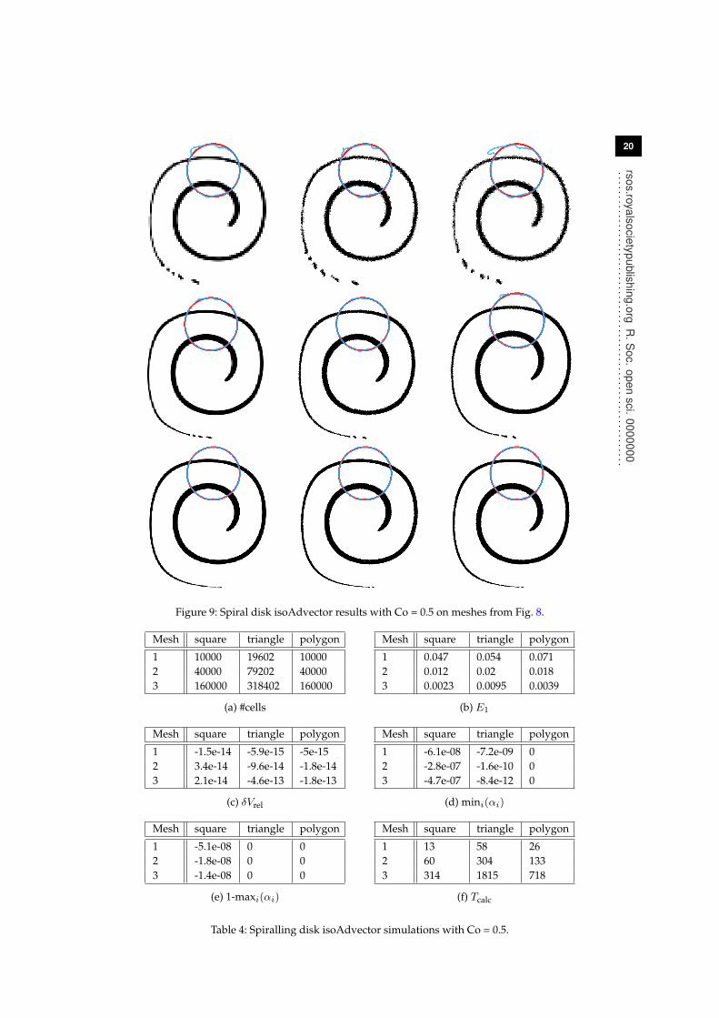
In Fig. 8 we show the square, triangle and polygon meshes in three different resolutionson which the isoAdvector method was tested. The results are shown in Fig. 9 using the samearrangement of the meshes. All simulations are run with Co = 0.5. In each panel, the exact initialand final interface shape is shown with a red circle overlaid with the α= 0.5 contour (blue) ofthe final (i.e. at time t= 8) volume fraction data. The spiral shaped volume of fluid at time t= 4,where it is maximally stretched, is also shown in each panel. All simulations show some degreeof pinching at t= 4. This occurs when the filament thickness reaches the cell size as is to beexpected. The phenomena is therefore most pronounced on the coarsest meshes. We note thatwhereas the exact mathematical solution does not pinch, the 0.5-contour of its volume fractionrepresentation will indeed pinch, if the mesh is coarse enough. As such, pinching does not have tobe an error. However, as droplets pinch off, and the local interface curvature becomes comparableto the cell size, the isofaces are not able to represent the significant interface curvature insidea cell. The isoface based approximation of the advection then becomes faulty, leading to errorsin the estimate of the droplet motion similar to those reported in [25]. The irreversibility of the

Figure 8: Meshes used to study spiralling disk case. Zoom on part of the initial interface. Exactcircular shape shown in red and 0.5-contour of volume fractions shown in blue.

20


.Soc.

opensci.

0000000..............................................................

1

Figure 9: Spiral disk isoAdvector results with Co = 0.5 on meshes from Fig. 8.

Mesh square triangle polygon

1 10000 19602 100002 40000 79202 400003 160000 318402 160000

(a) #cells


1 0.047 0.054 0.0712 0.012 0.02 0.0183 0.0023 0.0095 0.0039

(b) E1


1 -1.5e-14 -5.9e-15 -5e-152 3.4e-14 -9.6e-14 -1.8e-143 2.1e-14 -4.6e-13 -1.8e-13

(c) δVrel


1 -6.1e-08 -7.2e-09 02 -2.8e-07 -1.6e-10 03 -4.7e-07 -8.4e-12 0

(d) mini(αi)


1 -5.1e-08 0 02 -1.8e-08 0 03 -1.4e-08 0 0

(e) 1-maxi(αi)


1 13 58 262 60 304 1333 314 1815 718

(f) Tcalc

Table 4: Spiralling disk isoAdvector simulations with Co = 0.5.

21


.Soc.

opensci.

0000000..............................................................

1

Figure 10: Spiral disk simulation MULES results with Co = 0.1 on the three intermediate resolutionmeshes from Fig. 8.


E1 0.072 0.66 0.09δVrel 2.8e-14 -3.1e-14 -2e-15Tcalc 553 4151 1355

Table 5: Spiralling disk error measures for MULES with Co = 0.1 on intermediate meshes (tocompare with middle row in Fig. 9 and meshes 2 in Table 4).

introduced errors causes a distortion of the final disk in its upper region, which is made up of thepreviously pinched–off fluid.

The mesh sizes, error measures and calculation times are shown in Table 4. From theE1 valuesin Table 4, the orders of convergence with mesh refinement are calculated to be 1.9, 1.7 and 1.9 forthe square, triangle and polygon meshes, respectively. For a comparison, we show in Fig. 10 andTable 5 the results obtained with MULES on the intermediate resolution meshes of the three types,using Co = 0.1. For the square mesh, the MULES E1 error is ∼ 50% larger than the correspondingisoAdvector error. For the triangle mesh, the final interface is completely disintegrated. On thepolygon mesh, MULES also gives acceptable results, although the E1 error is 5 times larger thanthe isoAdvector error on the same mesh. In terms of calculation times, MULES is∼10 times slowerthan isoAdvector. This is in part because MULES is run with smaller time steps. However, wealso ran the simulations with Co = 0.5, in which case the MULES results on all three meshes werecompletely disintegrated like the triangle mesh solution in Fig. 10.

4.3 Sphere in steady uniform 3D flowIn this test we go back to a uniform flow, but now in 3D. The velocity is U = (0, 0, 1), and theinitial interface is a sphere of radius R= 0.25 centred at (0.5, 0.5, 0.5). The simulations are run onthree meshes consisting of 49.868, 343.441 and 1.753.352 random tetrahedra covering the domain,[0, 1]× [0, 1]× [0, 5]. The meshes and the 0.5-isosurface of the initial volume fraction data areshown in Fig. 11. The simulations are run with Co = 0.5 until t= 4, where the sphere has movedto (0.5, 0.5, 4.5). The results are show in Fig. 12 and in Table 6. In the top row of Fig. 12, weshow the exact final sphere (red) and the 0.5-isosurface of its volume fraction representation onthe three mesh resolutions. In the bottom row, we show the exact sphere (red) together with the0.5-isosurface of the final volume fraction data obtained with isoAdvector. As seen from Table 6,the E1 error on the coarsest mesh is fairly large. From Fig. 12 (lower left panel), we see that thislack of overlap is mainly due to an overestimation of the propagation speed rather than a lack ofability to retain the spherical interface shape. On the finer meshes E1 is reduced significantly, allthough the tendency to be slightly ahead of the exact solution is still visible in Fig. 12. The linear

22


.Soc.

opensci.

0000000..............................................................

Figure 11: Random tetrahedron meshes used for sphere in uniform flow test case. α= 0.5

isosurface shown for initial volume fraction data.

Figure 12: Sphere in uniform flow U = (0, 0, 1) on tetrahedral mesh at time t= 4. Top row: Exactsolution (red sphere) and its 0.5-isosurface on three different mesh resolutions. Bottom row: Exactsolution (red sphere) and 0.5-isosurface of the isoAdvector solution with Co = 0.5.

nCells E1 δVrel mini(αi) 1-maxi(αi) δWrel Tcalc

49.868 0.18 -2.8e-11 0 0 -0.033 11343.441 0.046 -7.8e-12 -6.9e-11 0 0.0067 1571.753.352 0.021 5.9e-11 -2.7e-09 0 0.0035 1411

Table 6: Sphere in uniform flow errors and calculation times for isoAdvector with Co = 0.5.

23


.Soc.

opensci.

0000000..............................................................

cell size is reduced by a factor 1.9 from the coarse to intermediate mesh, and by a factor 1.7 fromthe intermediate to fine. Based on these ratios, and the E1’s in the Table 6, the convergence orderis in the calculated to be in the range 2.6-3.2.

For comparison, we show in Fig. 13 and Table 7 the results obtained with MULES on the finestmesh running with Co = 0.1 and 0.5. In both cases the shape preservation is significantly worsethan the isoAdvector results. It is also noticeable that the MULES simulations with Co = 0.1 andCo = 0.5 are, respectively, 20 and 5 times slower than the corresponding isoAdvector simulationwith Co = 0.5.

Figure 13: Sphere in uniform flow U = (0, 0, 1) at time t= 4 on the finest tetrahedral mesh ofFig. 12. Left: Exact solution (red sphere) and 0.5-isosurface of MULES solution with Co = 0.5.Right: The same but with Co = 0.1.

Co E1 δVrel mini(αi) 1-maxi(αi) δWrel Tcalc

0.5 0.42 -4.5e-13 -5e-06 -1.9e-06 2 73060.1 0.29 -8.2e-13 0 9e-06 1.9 28686

Table 7: Sphere in uniform flow errors measures for MULES on the finest tetrahedron mesh.

4.4 Sphere in non-uniform 3D flowOur final test case is also in 3D, but now with a non-uniform velocity field. We adopt a setup oftenused to test surface smearing in 3D [18,26–28]. The domain is the unit box, and the initial interfaceis a sphere of radius R= 0.15 centred at (0.35, 0.35, 0.35). This surface is advected in the velocityfield,

u(x, y, z, t) = cos(2πt/T )

2 sin2(πx) sin(2πy) sin(2πz)

− sin(2πx) sin2(πy) sin(2πz)

− sin(2πx) sin(2πy) sin2(πz)

, (4.4)

where the period is set to T = 6. This flow stretches the sphere into a thin sheet creating twobending and spiralling “tongues”. The maximum deformation is reached at t= 1.5, where thetemporal cosine prefactor completely quenches the flow. From here on the flow reverses, and theinterface returns to its initial shape and position at time t= 3. In Fig. 14 the isoAdvector results areshown at time t= 1.5 in the top row, and at time t= 3 in the bottom row, on three cubic mesheswith dx= 1/64, 1/128 and 1/256. In the lower panels, the exact final spherical shape is also shown

24


.Soc.

opensci.

0000000..............................................................

Nx = 64t=

1.5

Nx = 128 Nx = 256t=

3

1Figure 14: α= 0.5 isosurfaces for sphere in non-uniform flow with Co = 0.5. Results for three meshresolutions are shown at the time of maximum strechting, t= 1.5, and at the final time, t= 3. Exactfinal solution is shown with red spheres.

Nx E1 δVrel mini(αi) 1-maxi(αi) δWrel Tcalc

64 0.22 -2.6e-13 0 0 0.5 173128 0.047 -2.6e-12 -2.1e-11 0 0.17 2626256 0.012 -1.6e-11 -8.1e-09 0 0.12 46706

Table 8: Error measures and calculation times for isoAdvector simulations in Fig. 14 of a spherein a 3D non-uniform flow on three cube meshes.

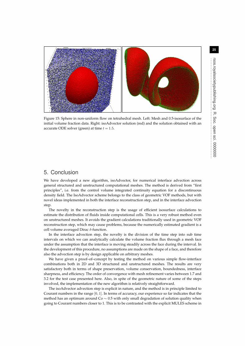
in red. From ODE calculations with the velocity field (4.4), we have measured the sheet thicknessat t= 1.5 to be ∼ 0.0063. This, and the fact that an edge can at most be cut once by the prescribedisosurface routine, explains why there are holes in the 0.5-isosurface of the volume fraction dataon the two coarsest mesh with dx≈ 0.016 and dx≈ 0.0078, and no wholes in the finest simulationwith dx≈ 0.0039. The error measures and calculation times for the three simulations are shownin Table 8. Based on theE1’s in this table, the order of convergence is calculated to be 2.3. We havealso performed this test on a mesh consisting of random tetrahedra. To get sufficient resolutionto avoid holes in the 0.5-isosurface of the solution, we used a mesh with 10.131.041 cells. A cutthrough this mesh and the 0.5-isosurface of the volume fraction representation of the initial sphereare shown in the left panel on Fig. 15. In the right panel, we show the isoAdvector solution attime t= 1.5, where the stretching is maximal. This panel also contains a solution obtained byintegrating the velocity field with a Runge-Kutta ODE solver for 160.000 points evenly distributedon the initial sphere (green dots). The visual impression from Fig. 15 is that there is a good matchbetween the ODE and the isoAdvector solutions. Due to the clipping procedure in the boundingstep, δVrel was 0.63% at time t= 3. It took ∼3 days to simulate until t= 3, and it is thereforeimpractical to do further testing of isoAdvector on such large meshes until the code has beenparallelised.

25


.Soc.

opensci.

0000000..............................................................

Figure 15: Sphere in non-uniform flow on tetrahedral mesh. Left: Mesh and 0.5-isosurface of theinitial volume fraction data. Right: isoAdvector solution (red) and the solution obtained with anaccurate ODE solver (green) at time t= 1.5.

5. ConclusionWe have developed a new algorithm, isoAdvector, for numerical interface advection acrossgeneral structured and unstructured computational meshes. The method is derived from “firstprinciples”, i.e. from the control volume integrated continuity equation for a discontinuousdensity field. The IsoAdvector scheme belongs to the class of geometric VOF methods, but withnovel ideas implemented in both the interface reconstruction step, and in the interface advectionstep.

The novelty in the reconstruction step is the usage of efficient isosurface calculations toestimate the distribution of fluids inside computational cells. This is a very robust method evenon unstructured meshes. It avoids the gradient calculations traditionally used in geometric VOFreconstruction step, which may cause problems, because the numerically estimated gradient is acell volume averaged Dirac δ-function.

In the interface advection step, the novelty is the division of the time step into sub timeintervals on which we can analytically calculate the volume fraction flux through a mesh faceunder the assumption that the interface is moving steadily across the face during the interval. Inthe development of this procedure, no assumptions are made on the shape of a face, and thereforealso the advection step is by design applicable on arbitrary meshes.

We have given a proof–of–concept by testing the method on various simple flow-interfacecombinations both in 2D and 3D structured and unstructured meshes. The results are verysatisfactory both in terms of shape preservation, volume conservation, boundedness, interfacesharpness, and efficiency. The order of convergence with mesh refinement varies between 1.7 and3.2 for the test case presented here. Also, in spite of the geometric nature of some of the stepsinvolved, the implementation of the new algorithm is relatively straightforward.

The isoAdvector advection step is explicit in nature, and the method is in principle limited toCourant numbers in the range [0, 1]. In terms of accuracy, our experience so far indicates that themethod has an optimum around Co ∼ 0.5 with only small degradation of solution quality whengoing to Courant numbers closer to 1. This is to be contrasted with the explicit MULES scheme in

26


.Soc.

opensci.

0000000..............................................................

OpenFOAM R©’s interFoam solver, which in our experience is limited to Co ≤ 0.1, if accuracy isimportant.3

The isoAdvector code is published [13] as an open source extension to OpenFOAM R©. It isour hope that the isoAdvector concept and code will be used, tested, and further developed bythe CFD community, and eventually result in improved simulation quality in the broad field ofapplications involving interfacial flows.

We note, that since the governing equation we solve is the passive advection equation fora scalar field in an solenoidal velocity field, the isoAdvector method may also find applicationswithin other branches of CFD, where the advected surface is not necessarily marking the interfacebetween two distinct fluids. There are many situations, where one needs to follow a passivetracer field, e.g. representing the concentration of some substance, which is immiscible with thesurrounding fluid. Another possible application could be in an Immersed Boundary Method,where the isoAdvector scheme could provide accurate estimates of the fluid-solid interface withincomputational cells.

We are currently parallelising the isoAdvector code, and the parallelised version will beavailable in a new release in the code repository [13]. Based on the interFoam solver inOpenFOAM, we are also working on a consistent coupling of isoAdvector with a pressure-velocity solver. The performance of the resulting new interfacial flow solver will be presented ina future paper. Finally we note that, due to its applicability on arbitrary meshes, the isoAdvectorcode can be coupled with an adaptive mesh refinement routine with only minor modifications.Such a coupling will also be investigated in future work.

AcknowledgmentThis work was sponsored by a Sapere Aude: DFF – Research Talent grant from The DanishCouncil for Independent Research | Technology and Production Sciences to JR (Grant–ID: DFF –1337-00118). The grant also covers all activities of HB and HJ in connection with the project. JRalso enjoys partial funding through the GTS grant to DHI from the Danish Agency for Science,Technology and Innovation. We would like to express our sincere gratitude for this support.JR is grateful to the following people for fruitful discussions and for help on improving theisoAdvector code: Tomislav Maric, Daniel Deising, and Holger Marschall from the MathematicalModeling and Analysis Group at the Center of Smart Interfaces, Technische UniversitätDarmstadt, Vuko Vukcevic3, Tessa Uroic3, Bjarne Jensen1, and Henrik Rusche from Wikki Ltd.

References1. G. Tryggvason, R. Scardovelli, and S. Zaleski, Direct Numerical Simulations of Gas–Liquid

Multiphase Flows.Cambridge University Press, Mar. 2011.

2. S. Popinet, “Gerris: a tree-based adaptive solver for the incompressible Euler equations incomplex geometries,” Journal of Computational Physics, vol. 190, pp. 572–600, Sept. 2003.

3. The OpenFOAM Foundation, “Openfoam.” www.openfoam.org.4. H. G. Weller, G. Tabor, H. Jasak, and C. Fureby, “A tensorial approach to computational

continuum mechanics using object-oriented techniques,” Computers in Physics, vol. 12,pp. 620–631, Nov. 1998.

5. C. Hirt and B. Nichols, “Volume of fluid (VOF) method for the dynamics of free boundaries,”Journal of Computational Physics, vol. 39, pp. 201–225, Jan. 1981.

6. S. S. Deshpande, L. Anumolu, and M. F. Trujillo, “Evaluating the performance of the two-phase flow solver interFoam,” Computational Science & Discovery, vol. 5, p. 014016, Jan. 2012.

7. H. T. Ahn and M. Shashkov, “Multi-material interface reconstruction on generalizedpolyhedral meshes,” Journal of Computational Physics, vol. 226, pp. 2096–2132, Oct. 2007.

3It should be mentioned that from OpenFOAM R© version 2.3.0 a new semi-implicit MULES scheme is introduced to solvesome of the issues with boundedness, stability, and accuracy for large Courant numbers. The literature documenting the ideasbehind and the performance of this new method is, however, still very sparse.

www.openfoam.org

27


.Soc.

opensci.

0000000..............................................................

8. J. Hernández, J. López, P. Gómez, C. Zanzi, and F. Faura, “A new volume of fluid methodin three dimensionsUPart I: Multidimensional advection method with face-matched fluxpolyhedra,” International Journal for Numerical Methods in Fluids, vol. 58, no. 8, pp. 897–921,2008.

9. J. López, C. Zanzi, P. Gómez, F. Faura, and J. Hernández, “A new volume of fluid methodin three dimensionsUPart II: Piecewise-planar interface reconstruction with cubic-Bézier fit,”International Journal for Numerical Methods in Fluids, vol. 58, no. 8, pp. 923–944, 2008.

10. C. B. Ivey and P. Moin, “Conservative volume of fluid advection method on unstructuredgrids in three dimensions,” Center for Turbulence Research, Annual Research Briefs, 2012.

11. T. Maric, H. Marschall, and D. Bothe, “voFoam - A geometrical Volume of Fluid algorithmon arbitrary unstructured meshes with local dynamic adaptive mesh refinement usingOpenFOAM,” arXiv:1305.3417 [physics], May 2013.arXiv: 1305.3417.

12. B. Xie, S. Ii, and F. Xiao, “An efficient and accurate algebraic interface capturing methodfor unstructured grids in 2 and 3 dimensions: The THINC method with quadratic surfacerepresentation,” International Journal for Numerical Methods in Fluids, vol. 76, pp. 1025–1042,Dec. 2014.

13. Johan Roenby, “isoAdvector.” www.github.com/isoAdvector.14. C. Kitware, Sandia National Labs, “Paraview.” www.paraview.org.15. S. Muzaferija, M. Peric, P. Sames, and T. Schellin, “A two-fluid navier-stokes solver to simulate

water entry,” in Proceedings of the 22nd symposium on naval hydrodynamics, Washington, DC,pp. 277–289, 1998.

16. O. Ubbink and R. Issa, “A Method for Capturing Sharp Fluid Interfaces on Arbitrary Meshes,”Journal of Computational Physics, vol. 153, pp. 26–50, July 1999.

17. K. B. Nielsen, Numerical prediction of green water loads on ships.PhD thesis, Technical University of Denmark, Department of Mechanical Engineering, 2003.

18. M. Jemison, E. Loch, M. Sussman, M. Shashkov, M. Arienti, M. Ohta, and Y. Wang, “A CoupledLevel Set-Moment of Fluid Method for Incompressible Two-Phase Flows,” Journal of ScientificComputing, vol. 54, pp. 454–491, Feb. 2013.

19. H. T. Ahn and M. Shashkov, “Adaptive moment-of-fluid method,” Journal of ComputationalPhysics, vol. 228, pp. 2792–2821, May 2009.

20. V. Le Chenadec, “A 3d Unsplit Forward/Backward Volume-of-Fluid Approach and Couplingto the Level Set Method,” Journal of Computational Physics, vol. 233, no. 1, pp. 10–33, 2013.

21. D. J. E. Harvie, “A new volume of fluid advection algorithm: The Stream scheme,” Journal ofComputational Physics, vol. 162, no. 1, pp. 1–32, 2000.

22. W. J. Rider and D. B. Kothe, “Reconstructing Volume Tracking,” Journal of ComputationalPhysics, vol. 141, pp. 112–152, Apr. 1998.

23. M. Rudman, “A volume-tracking method for incompressible multifluid flows with largedensity variations,” INTERNATIONAL JOURNAL FOR NUMERICAL METHODS IN FLUIDS,vol. 28, no. 2, pp. 357–378, 1998.

24. M. Rudman, “Volume-tracking methods for interfacial flow calculations,” International Journalfor Numerical Methods in Fluids, vol. 24, no. 7, pp. 671–691, 1997.

25. G. Cerne, S. Petelin, and I. Tiselj, “Numerical errors of the volume-of-fluid interface trackingalgorithm,” International Journal for Numerical Methods in Fluids, vol. 38, pp. 329–350, Feb. 2002.

26. S. Shin, I. Yoon, and D. Juric, “The Local Front Reconstruction Method for direct simulationof two- and three-dimensional multiphase flows,” Journal of Computational Physics, vol. 230,pp. 6605–6646, July 2011.

27. P. Liovic, M. Rudman, J.-L. Liow, D. Lakehal, and D. Kothe, “A 3d unsplit-advection volumetracking algorithm with planarity-preserving interface reconstruction,” Computers & Fluids,vol. 35, pp. 1011–1032, Dec. 2006.

28. D. Enright, F. Losasso, and R. Fedkiw, “A fast and accurate semi-Lagrangian particle level setmethod,” Computers & Structures, vol. 83, pp. 479–490, Feb. 2005.

www.github.com/isoAdvector

www.paraview.org

a computational method for sharp interface advection*

Documents