A COMPUTER SIMULATION OF REACTION PLANE MEMORY

VIA QUASIPARTICLE DYNAMICS

b y

John Chun Kit Wong

B.Sc. (Hons.), Simon Fraser University, 1985.

THESIS SUBMITTED IN PARTIAL FULFILLMENT OF

THE REQUIREMENTS FOR THE DEGREE OF

MASTER OF SCIENCE

in the - Department

of

PHYSICS

@ John Chun Kit Wong 1990

SIMON FRASER UNIVERSITY

January, 1990

All rights reserved. This work may not be

reproduced in whole or in part, by photocopy

or other means, without permission of the author.

APPROVAL

Name: John Chun Kit Wong

Degree: M.Sc. (Physics)

Title of Thesis: A Computer Simulation of Reaction Plane Memory

via Quasiparticle Dynamics.

Examining Committee:

Chairman: E.D. Crozier

7 -

D.H: 'Boa1 Professor

Senior Supervisor

- -

Profess Department of Chemistry

K.S. Viswanathan Professor

R.M. Woloshyn Adjunct Professor External Examiner

PARTIAL COPYRIGHT LICENSE

I hereby g ran t t o Simon Fraser U n i v e r s i t y the r i g h t t o lend

my thes is , p r o j e c t o r extended essay ( t h e t i t l e o f which i s shown below)

t o users o f the Simon Fraser University L ib ra ry , and t o make p a r t i a l o r

s i n g l e copies on l y f o r such users o r I n response t o a request from the

l i b r a r y of any o the r u n i v e r s i t y , o r o the r educat ional i n s t i t u t i o n , on

i t s own behalf o r f o r one o f I t s users. I f u r t h e r agree t h a t permission

f o r m u l t i p l e copying o f t h i s work f o r scho la r l y purposes may be granted

by me o r the Dean o f Graduate Studies. I t i s understood t h a t copying

o r p u b l l c a t l o n o f t h i s work f o r f i n a n c i a l ga ln s h a l l not be al lowed

w i thout my w r i t t e n permission.

T i t l e o f Thesis/Project/Extended Essay

A Corrrputer Simulation of Reaction Plane mry

v ia Quasipar t ic le Dynamics.

Author:

( s i gna tu re )

John Chun K i t Wong

(da te )

ABSTRACT

Quasiparticle Dynamics, a computer simulation for nuclear reactions,

is used to investigate reaction plane memory in intermediate energy

heavy ion collisions. In particular, extensive simulations involving

the generation of more than 21,000 events are performed for

14N+154Sm at 35 A.MeV. The gamma ray circular polarization, as a

function of trigger mass, energy and angle, is shown to be a measure

of the correlation between the trigger plane and the reaction plane.

Calculations of the inclusive particle spectrum, as well as circular

polarization, are compared with experiment and the Boltzmann-

Uehling-Uhlenbeck model. The dependence of the calculated

observables on the assumed in-medium nucleon-nucleon cross

section is also investigated.

ACKNOWLEDGEMENTS

I would like to thank my supervisor David Boa1 for giving me the

problem to work on and for guiding me all the way. I must express

my gratitude to the Natural Sciences and Engineering Research

Council of Canada and the Department of Physics for financial

support.

TABLE OF CONTENTS

. . APPROVAL 11

ABSTRACT iii

ACKNOWLEDGEMENTSp iv

TABLE OF CONTENTS- v

LIST OF FIGURES- vii

LIST OF TABLES viii

1 introduction^ - 1

1.2 Brief Review of Computer Simulations In Nuclear Reaction Studiess2

1.3 Boltzmann-Uehling-Uhlenbeck Equation-5

1 .4 Quasiparticle Dynamics17

1.5 Gamma Ray Circular Polarizationp8

2 Quasiparticle Dynamics81 3

2.1 I n t r o d u c t i ~ n ~ ~ 3

2.2 Pauli Potentialpl 4

2.3 Nuclear Interactionc17

2.4 Nucleon-Nucleon Collision Termc2 2

2.5 Comparison Between BUU and QPDp2 3

3 Single Particle Inclusive Spectras2 6

3.1 Introduction12 6

3.2 Details of the Simulationss2 6

3.3 Properties of the Residual Reaction Products-2 8

3.4 Single Particle Inclusive Spectra for Light Particles-3 3

3.5 Comparison Between QPD and BUU C a l c u l a t i 0 n s ~ 4 4

4 Gamma Ray Circular P o l a r i z a t i o n 4 8

4.1 I n t r o d u c t i o n 4 8

4 . 2 M e t h o d o l o g y 4 9

4 . 3 Results of the C a l c u l a t i o n 5 3

4 . 4 Comparison with BUU C a l c u l a t i o n s 6 3

4 . 5 Microscopic Dynamics of the Collision P r o c e s s 6 4

LIST OF TABLES

3.1 Differential multiplicities of the fragments at different combinations of emission angle and in-medium NN cross sectionl... 6

4.1 Gamma ray circular polarization associated with nucleon triggers predicted by the QPD and BUU m o d e l s . 5 3

4.2 Circular polarization predicted by the BUU model using different (TNN at a fixed impact parameter of b = 6.5 fm. The nucleon trigger angle is 60"- 6 4

vii

LIST OF FIGURES

1.1 Sign convention for the deflection angles of the particles emittedsl 1

3 .1 Predicted heavy nucleus mass yields for N+Sm at 35 A.MeV-3 1

3.2 Predicted fractional distribution of excitation energy for the 163H0 nucleus calculated from simulation of N+Sm at 35 A.MeV, as in Fig. 3.11 3 2

3.3 Comparison of experimental data with QPD predictions for proton emission at 30' in N+Sm at 35 A.MeV-3 8

3.4 Similar to Fig. 3.3 but for proton emission at 60"-3 9

3 .5 Similar to Fig. 3.3 but for deuteron emission at 30'-40

3.6 Similar to Fig. 3.3 but for deuteron emission at 6 0 ' 4 1

3.7 Similar to Fig. 3.3 but for triton emission at 3 0 ' 4 2

3 .8 Similar to Fig. 3.3 but for triton emission at 6 0 ' 4 3

3 .9 Comparison of BUU calculations with QPD predictions for nucleon emission at 30" in N+Sm at 35 A.MeV 4 6

3 .10 Similar to Fig. 3.9 but for nucleon emission at 60' 4 7

4.1 Sign convention for vectors and planes involved in the circular polarization determinationn5 1

4 .2 Predicted trigger mass and energy dependence of circular polarization observed at 30" for the reaction N+Sm at 35 A.MeV, oNN=28 mb and averaged over impact parameter-5 6

4.3 Predicted proton trigger emission energy dependence of circular polarization shown at both 30' and 60". Other conditions are as Fig. 4 . 2 5 7

4 .4 Similar to Fig. 4.3 but for deuteron t r i g g e r s 5 8

4.5 Comparison of simulation and experiment for proton triggered events at 30" 5 9

4.6 Similar to Fig. 4.5 but for proton triggered events at 60"- 6 0

4.7 Similar to Fig. 4.5 but for deuteron triggered events at 3 0 ' 6 1

4.8 Similar to Fig. 4.5 but for deuteron triggered events at 60•‹__62

. . . V l l l

4 .9 Distribution of impact parameter b for proton triggers and a range of energies96 8

4.10 Similar to Fig. 4.9 but for deuteron triggers-6 9

4 .1 1 Relative dispersion of the orientation of the reaction plane with respect to the trigger plane shown as a function of circular p o l a r i z a t i o n 7 0

Chapter One

Introduction

1.1 Introduction

In heavy ion collisions, nuclear matter is usually compressed at the

early stage of the reaction because of the interpenetration of the

projectile and the target. Nucleon-nucleon collisions cause both the

temperature and the entropy of the system to rise. The state of

compression can only last for a very short time, typically about

30 fm/c= 10-22 second. Then the system disassembles. The number

of nucleon-nucleon collisions falls quickly and the entropy changes

slowly. During the expansion phase of the reaction, the density

decreases to a value where the nucleons are no longer interacting.

This density is called the freeze-out density. In heavy ion reaction

experiments, the detectors can only measure the experimental

observables long after this stage. To understand the whole process

of a nuclear reaction requires detailed analysis of the experimental

observables. Reviews of heavy ion collision phenomena can be found

in References 1 to 3.

Computer simulations have been used for more than a quarter of a

century to study some aspects of nuclear physics.4 In nuclear

reaction experiments, the observables such as momenta and energies

of particles emitted are measured a long time after the reaction

begins. One cannot understand the step-by-step mechanism of the

reaction from the measured observables alone. The advantage of

computer simulation is that one can study the reaction at any time

step throughout the whole reaction process. Further, experiments

have no control on either the magnitude or the direction of the

impact parameter between the projectile and the target in heavy ion

reactions. In a computer simulation, the impact parameter can be set

at whatever value desired.

In many heavy ion collisions, the number of nucleons involved will

be in the order of 100 and the reaction cannot be easily described in

analytical form. The fermionic nature of nucleons requires that the

antisymmetric wave function of a nucleus will have at least A! terms.

There will be many more terms if one wants to determine the

expectation value of observables such as kinetic energy. It would be

computationally demanding to determine the time evolution problem

of any observable by numerically propagating the nuclear wave

function except for very light nuclei. Many models have been

developed to attempt to reduce the many-body problem to a

computationally manageable scale. In the next section, a brief

review of computer simulations in nuclear studies is discussed.

1.2 Brief Review of Computer Simulations In Nuclear

Reaction Studies

Several different models have been developed in the history of

computer simulation of heavy ion collisions. One of the earliest

methods of simulating nuclear reactions is by modelling the reaction

using the equations of hydrodynamics. If the mean free path of a

nucleon in nuclear matter is sufficiently short, then a local

equilibrium may be established within the reaction zone and the

region may evolve according to hydrodynamics. The nucleon mean

free path is estimated to be of the order of the internucleon spacing.5

One can determine the trajectory of a nuclear reaction by solving the

hydrodynamic equations governing the time evolution of quantities

such as the energy density, number density and momentum

density.6 The attraction of hydrodynamics is the simplicity of its

ingredients: conservation laws and an equation of state. Several

numerical solutions of the hydrodynamic equations for heavy ion

collisions have been performed.6 However, hydrodynamics demands

that individual nucleon-nucleon collisions are frequent enough to

maintain a local equilibrium during the course of a reaction. This

method is not applicable to intermediate energy heavy ion collision.

A more exclusive model than hydrodynamics is the Intranuclear

Cascade Model (INC) in which nucleons are propagated in space by

means of classical mechanics.' The motion of the nucleons is a

straight line unless it is affected by a nucleon-nucleon collision,

which occurs if the distance of closest approach of two nucleons falls

below the classical scattering radius determined by the measured

nucleon-nucleon (NN) cross section. This model is computationally

fast and simple. Furthermore, it is a true A-body problem. It has

been used to address a number of questions about the internal

dynamics of a reaction such as the production of entropy in central

collisions . 8 However, neither the nuclear potential nor the Pauli

Exclusion Principle are considered in this model, and it cannot be

used to describe fragment formation in nuclear reactions.

For reactions at low energy, i.e., the projectile kinetic energy per

nucleon is a few MeV above the Coulomb barrier, many of the

individual nucleon-nucleon collisions are Pauli-blocked. The reaction

is dominated by the nuclear mean field. Nucleus-nucleus collisions at

small impact parameter lead to complete fusion of the projectile and

the target. An equilibrated compound nucleus is formed. The

deexcitation of the compound nucleus is by emission of particles and

photons. At large impact parameters, the collisions are dominated by

quasi-elastic reactions. At intermediate impact parameter collisions,

the two nuclei largely retain their form but there is a large

momentum and energy transfer.2

Some aspects of the nuclear reactions at low energy can be described

by the Vlasov equation9 which is the Boltzmann equation without the

collision term:

where f(r,p,t) is the one-body phase space density and U is the

nuclear potential function. However, since it neglects nucleon-

nucleon collisions, the Vlasov equation cannot be used to describe

reactions at higher energies.

For intermediate energy reactions, the projectile kinetic energy per

nucleon is in the range of 20 to 200 MeV. The relative velocity of

the two colliding nuclei in this range of energies is comparable in

magnitude to the Fermi velocity in nuclear matter, ~ ~ ~ 0 . 3 ~ .

In intermediate energy nuclear reaction, the energy is not high

enough that the nuclear mean field and the Pauli exclusion principle

can be neglected nor is it low enough that most of nucleon-nucleon

collisions can be ignored because of Pauli blocking factor.

1.3 Boltzmann-Uehling-Uhlenbeck Equation

One way of addressing the intermediate energy nuclear reaction

problem is by solving the Boltzmann equation for the single particle

phase space distribution f(r,p, t). The equation includes both a force

term, given by the gradient of the mean field potential, and also a

collision integral term. However, this method is not very appropriate

because effects such as Pauli blocking arising from nucleon-nucleon

collisions are excluded. Therefore the nucleon-nucleon collision term

should include the Pauli blocking factor for fermions as suggested by

Nordheimlo and Uehling and Uhlenbeck.11 An equation resembling

the classical Boltzmann equation has been developed for fermion

distributions and is known as the Boltzmann-Uehling-Uhlenbeck

(BUU) equation:

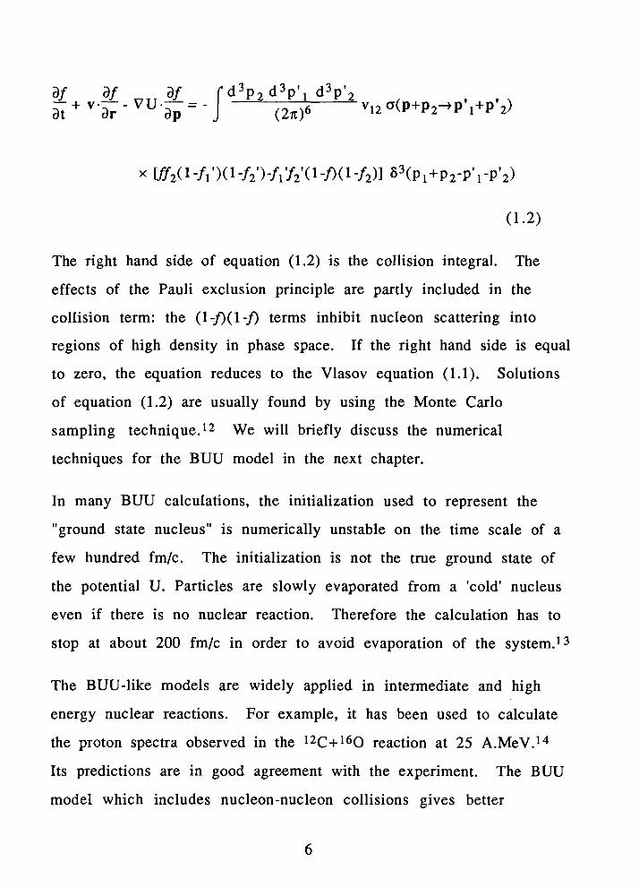
The right hand side of equation (1.2) is the collision integral. The

effects of the Pauli exclusion principle are partly included in the

collision term: the (1-f)(l -f) terms inhibit nucleon scattering into

regions of high density in phase space. If the right hand side is equal

to zero, the equation reduces to the Vlasov equation (1.1). Solutions

of equation (1.2) are usually found by using the Monte Carlo

sampling technique.12 We will briefly discuss the numerical

techniques for the BUU model in the next chapter.

In many BUU calculations, the initialization used to represent the

"ground state nucleus" is numerically unstable on the time scale of a

few hundred fm/c. The initialization is not the true ground state of

the potential U. Particles are slowly evaporated from a 'cold' nucleus

even if there is no nuclear reaction. Therefore the calculation has to

stop at about 200 fm/c in order to avoid evaporation of the system.13

The BUU-like models are widely applied in intermediate and high

energy nuclear reactions. For example, it has been used to calculate

the proton spectra observed in the l2C+l60 reaction at 25 A.MeV.14

Its predictions are in good agreement with the experiment. The BUU

model which includes nucleon-nucleon collisions gives better

predictions for intermediate energy heavy ion reactions than the

Vlasov equation. For example, a comparison between the Vlasov and

the BUU equations of the momentum space distribution for a central

Ar+Ca collision at 137 A.MeV has been made.15 In the Vlasov

approach, the final momentum distribution is still fairly close to that

of the initial projectile and target, i.e., the nuclei are largely

transparent to each other. On the other hand, the BUU approach

shows a much larger change of the momentum distribution, and is in

closer agreement with experiment. Discussion about the applications

of the BUU model can be found in review articles Refs. 1-4.

1.4 Quasiparticle Dynamics

The BUU model is a one-body model. The correlations between

nucleons have to be incorporated in a model-dependent fashion. For

example, a number of assumptions must be made in order to extract

fragments from the one-body distribution (we will discuss these

aspects in Chapter Three.)

In the time since the BUU model was developed, a considerable

amount of effort16 has gone into developing simulations for many-

particle distributions. These simulations include correlations

between nucleons and so incorporate fragment emission from heavy

ion reactions without further assumptions. One such model is the

Quasiparticle Dynamics model,l7 which is Hamiltonian-based yet

includes a stochastic nucleon-nucleon collision term.

In the Quasiparticle Dynamics model, each nucleon is represented by

a Gaussian wavepacket of width lla in coordinate space. The

degrees of freedom for the equations of motion are taken to be ex>

and cp>, the expectations of the individual wavepackets. Hence, each

nucleon is represented by a quasiparticle whose phase space

coordinates R and P are cx> and ep> respectively.

The wavepackets are not used to form an antisymmetric

wavefunction but a momentum-dependent potential acting pairwise

between the quasiparticles is used to incorporate many of the effects

on the fermions' energies arising from antisymmetrization. The

complete Hamiltonian of the system also includes terms representing

the nuclear interaction and the coulomb interaction. In Chapter Two,

we give a brief description of the development of the QPD model.

In Chapter Three, we use the Quasiparticle Dynamics (QPD) model to

simulate the reaction 14N+154Sm at 35 A.MeV. The properties of the

residual nuclei and the single particle spectra are studied. The

predicted spectra are compared with experiment and results from a

BUU calculation.

1.5 Gamma Ray Circular Polarization

One of the features of intermediate energy nuclear reactions is the

incomplete fusion reaction. By definition, complete fusion reactions

involve the projectile and the target completely fusing together and

the momentum of the projectile being transferred to the composite

system. The life-time of the compound nucleus is long enough that

the internal degrees of freedom are equilibrated and memory of the

entrance channel is lost. Particles are emitted by evaporation and

their distribution is isotropic in the nucleus-nucleus center-of-mass

frame. The velocity distribution of the residual nuclei is centered

about the center-of-mass of the system.

Incomplete fusion reactions denote processes in which some particles

are emitted prior to the complete equilibration of the composite

system. Those particles are called nonequilibrium particles, and are

more energetic than those evaporated from the equilibrated nucleus.

The angular distributions of the emitted particles are usually not

isotropic in the center-of-mass frame. In the laboratory frame, the

nonequilibrium light particle spectra are forward peaked. (See, for

example, data summarized in Refs. 1-3.)

Experimental evidence18 indicates that nonequilibrium particle

emission in an incomplete fusion reaction exhibits preferential

emission in the reaction plane which is perpendicular to the orbital

angular momentum, Ji, of relative motion between projectile and

target nuclei. The reaction plane is defined by the impact parameter

vector, b , and momentum vector of the beam, ki, where Ji is defined

as bxki. Tsang and co-workers detected light particles in coincidence

with two binary fission fragments for 14N induced reactions on 197Au

at 30 A.MeV incident kinetic energy.18 The two detected coincident

fission fragments and the beam form the fission plane which is

perpendicular to the orbital momentum of the fissioning nucleus. For

simplicity, the intrinsic spins of the projectile and target nuclei and

the angular momentum of particles emitted prior to fission are

neglected. In this approximation, the total angular momentum of the

fissioning nucleus is equal to the orbital angular momentum of

relative motion between projectile and target nuclei. Therefore, the

fission plane is approximately coplanar with the reaction plane. The

light particles detected in the fission plane are called 'in-plane'

particles while those detected perpendicular to the fission plane are

called 'out-of-plane' particles. The ratio of particles emitted out-of-

plane to those emitted in-plane is less than one. Thus the

experiment shows preferential emission of light particles in the

reaction plane.

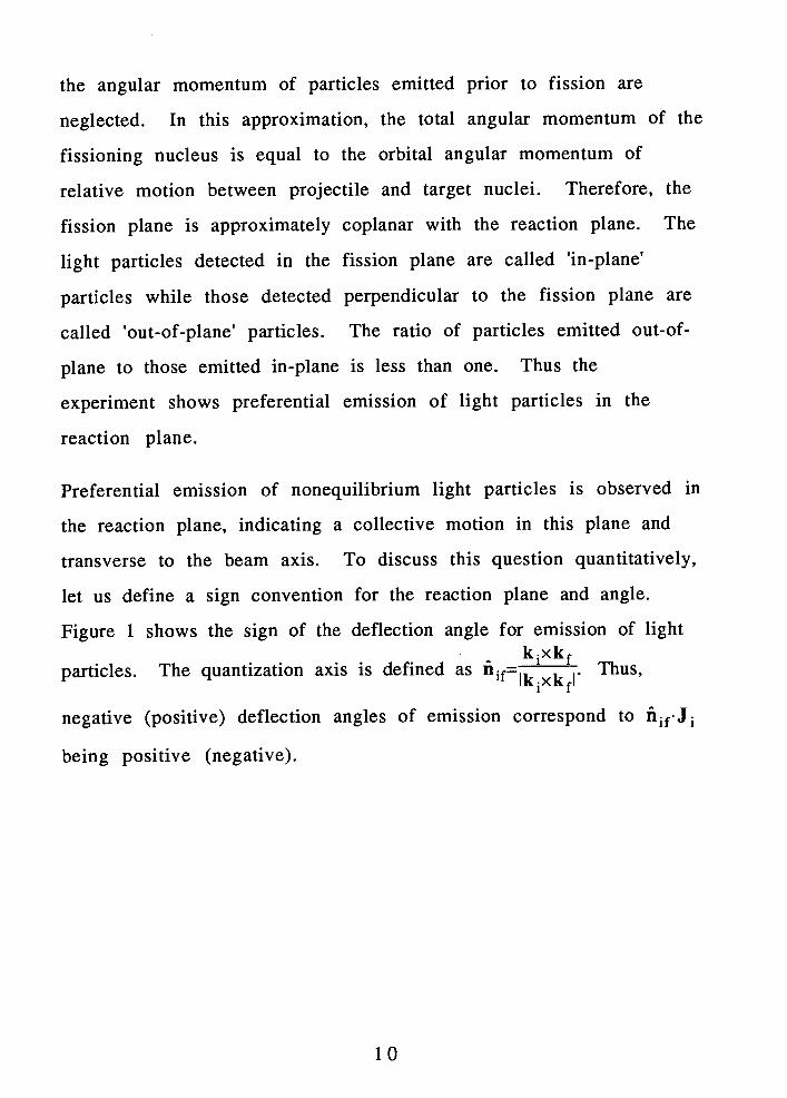
Preferential emission of nonequilibrium light particles is observed in

the reaction plane, indicating a collective motion in this plane and

transverse to the beam axis. To discuss this question quantitatively,

let us define a sign convention for the reaction plane and angle.

Figure 1 shows the sign of the deflection angle for emission of light kixkf

particles. The quantization axis is defined as i f7kixkfr

Thus,

negative (positive) deflection angles of emission correspond to hi f -J i

being positive (negative).

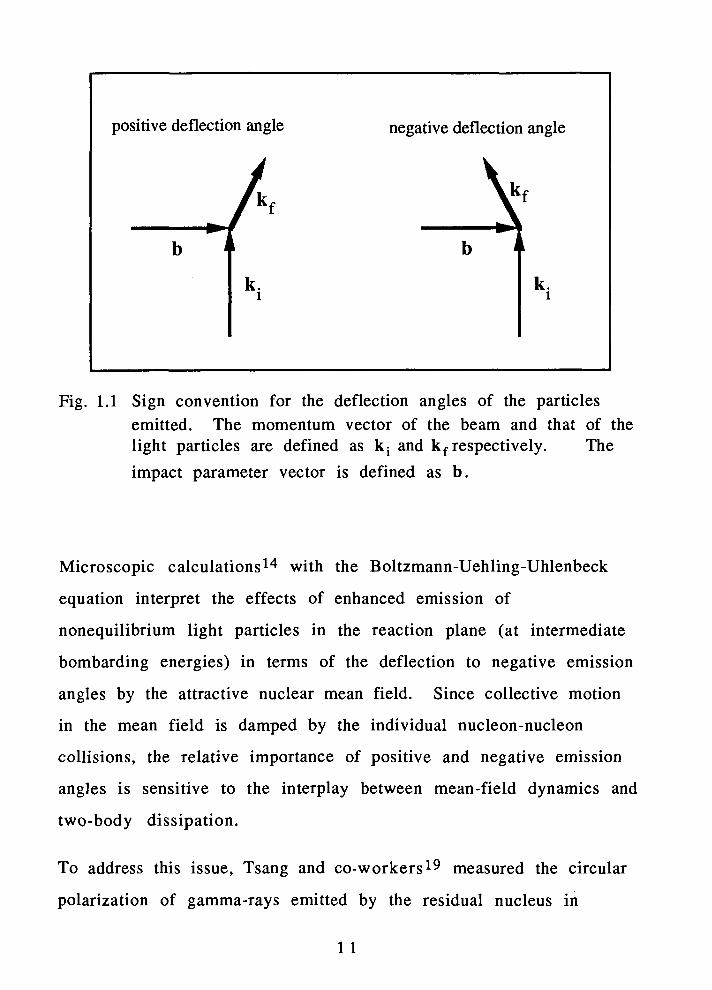
I positive deflection angle negative deflection angle

I Fig. 1.1 Sign convention for the deflection angles of the particles

emitted. The momentum vector of the beam and that of the light particles are defined as k i and kfrespectively. The

impact parameter vector is defined as b .

Microscopic calculationsl4 with the Boltzmann-Uehling-Uhlenbeck

equation interpret the effects of enhanced emission of

nonequilibrium light particles in the reaction plane (at intermediate

bombarding energies) in terms of the deflection to negative emission

angles by the attractive nuclear mean field. Since collective motion

in the mean field is damped by the individual nucleon-nucleon

collisions, the relative importance of positive and negative emission

angles is sensitive to the interplay between mean-field dynamics and

two-body dissipation.

To address this issue, Tsang and co-workers19 measured the circular

polarization of gamma-rays emitted by the residual nucleus in

coincidence with nonequilibrium light particle triggers for the

reaction 14N on 154Sm. The triggers are measured at polar angles of

30' and 60' with respect to the beam. The photons are detected

around the quantization axis. The sign of the gamma ray circular

polarization follows the sign of the average emission angle of

nonequilibrium light particles. Since light particles are

preferentially emitted in the reaction plane, the quantization axis

will be aligned with the angular momentum, J, of the heavy residue.

Semiclassically, the photon's spin will be parallel to the spin of the

residue. Therefore, positive circular polarization corresponds to

negative deflection and an attractive mean field.

Positive circular polarizations are observed for all light particle

triggers at both angles. The magnitude of the measured polarization

increases with increasing energy and mass of the triggers. This

experiment establishes the preferential emission of nonequilibrium

light particles to negative emission angles, consistent with an

attractive nuclear mean field calculated by the BUU model and with

measurements at lower energies.20

In Chapter Four, we use the QPD model to calculate the sign and the

magnitude of the gamma ray circular polarization in coincidence with

the light particle triggers. The results are compared with experiment

and the BUU code. We also study the microscopic dynamics of the

nucleus-nucleus collision process. Finally, our conclusions and

discussion are included in Chapter Five.

Chapter Two

Quasiparticle Dynamics

2.1 Introduction

On a quantum mechanical level, the fermionic nature of nucleons

demands that a nuclear wave function has to be antisymmetrized.

Thus there will be A! components to the wave function for a single

Slater determinant of a single nucleus of A nucleons. For all but the

lightest nuclei, it is impossible for existing computers to handle any

time evolution problem in nuclear reactions by propagating the

nuclear wave functions. Thus it is difficult to find a model to

describe nuclei in an efficient manner in computer simulations.

One method of tackling the problem is to find a classical potential

which can incorporate some of the effects of antisymmetrization. In

the Quasiparticle Dynamics (QPD) model,l7 the classical potential

(referred to as the Pauli potential) is obtained from evaluating the

expectation value of the kinetic-energy operator for a specific

nuclear wave function. Then the nuclear and Coulomb terms are

added to the potential such that the Hamiltonian of the system

involves A2 terms. With this simplification, systems with several

hundred nucleons can be investigated by computer simulation.

The layout of this chapter is as follows: In Section 2.2 the derivation

of the Pauli potential in QPD is described. The properties of ground

state nuclei in QPD are discussed in Section 2.3. In Section 2.4 the

nucleon-nucleon collision term is discussed. Finally, the differences

between BUU and QPD are compared in Section 2.5.

2.2 Pauli Potential

One of the effects of Fermi-Dirac statistics is that the ground state of

a fermion system has to have a non-zero expectation value of the

kinetic energy operator:

where the mass of the nucleon, m, is assigned to be 938.9 MeV. One

can see that there are at least A(A!)2 terms in equation (2.1) for a

nucleus with A nucleons, if YgeS. is antisymmetric. It is

computationally prohibitive to propagate equation (2.1) for all but

light nuclei. The motivation for the Quasiparticle Dynamics model is

to try to seek approximations to express equation (2.1) in terms of a

two-body interaction between the nucleons. With the approximation,

the number of terms for the kinetic energy expression (2.1) is A2

instead of A(A!)2.

In QPD, each nucleon is taken to have a wave packet which is

Gaussian in form

This wave packet is centered at ra and has an average momentum pa.

The two-particle antisymmetrized wave function formed from two of

these wave packets is

The total kinetic energy of a two-body system described by Yab is

whe re

The 3a2h2 term is a result of the uncertainty principle that the wave

packet is not a delta function in momentum. The last term of

equation (2.4) can be identified as a two-body potential between

quasiparticles with phase-space coordinates @,,pa) and (rb,pb). Thus,

in QPD the term

is identified as a candidate form for the Pauli potential between

classical quasiparticles which represent fermions. The Pauli potential

vanishes when the quasiparticles are well separated in phase space

and is repulsive for finite separation in phase space. A system of

quasiparticles interacting via the Pauli potential has features17 which

resemble the behavior of a many-particle Fermi gas.

The energy of a system of particles interacting via equation (2.5) (the

analogue of the free particle Fermi gas) is

whe re

The quasiparticles in the system hav e labels 1 and m.

Consider that the quasiparticles of a many-body system are placed in

a simple cubic lattice with lattice spacing a. If a a > > l , then the sites

are decoupled and the ground state has kl=0 for all I. However, this

is not the case for smaller separation. One can show17 that kl=0 is

not a global minimum of E for aac2.2, and therefore there exists a

ground state of the system at some nonzero kl.

Having found that the ground state of a system of quasiparticles has

non-zero kinetic energy, one can estimate a in equation (2.5) by

equating the ground state energy of a system of quasiparticles on a

simple cubic lattice with that of an ideal Fermi gas at the same

density. However, one finds that equation (2.5) always

underestimates the energy of a Fermi gas for all a. This arises

because only two-body terms in the Pauli potential have been used

in evaluating the kinetic energy of the many-body system.

Therefore, the strength of the Pauli potential has to be rescaled in

order to approximate the energetics of the three- and higher-body

terms. The Pauli potential is then rewritten as

where V, is the scaling factor. The two parameters of the Pauli

potential, V, and a, are fixed by equating the ground-state energy of

a system of quasiparticles on a simple cubic lattice with that of an

ideal Fermi gas at the same density over the density range of

interest. The best fit of V, and a is found to be 1.9 and 112 fm-1

respectively.

To summarize, the Pauli potential is a classical potential that

incorporates some of the properties of a system of non-interacting

fermions. Its use allows the reduction in the number of terms in an

A-body fermion Hamiltonian from A(A!)2 to A2.

2.3 Nuclear Interaction

In addition to the Pauli potential, the Hamiltonian of a nucleus must

include terms arising from the strong and electromagnetic

interaction. The nuclear potential energy density is taken to have

the following form:17

where p is the local density at coordinate r , and po is the density of

normal nuclear matter (taken to be 0.17 fm-3 here). The third term

is used to describe the isospin dependence of the nuclear force and is

a function of the local proton density, pp, and the local neutron

density, pn. The last term depends on the gradient of the density.

The density of the system is taken to be the direct sum of the

density of each quasiparticle pi, such that

This expression assumes that the cross terms in the X * X product of

antisymmetrized single-particle wave functions cancel.

Defining (X)i = Ipi(r) X d3r, equation (2.8) becomes

All summations but the second one involve of the order of terms.

There are A3 terms in the summation over (p2/po2). Therefore it is

approximated as

which involves A2 terms. The second term of equation (2.11)

vanishes for uniform nuclear matter. However, omission of this term

allows unphysical density fluctuations to develop and can lead to

ground state instabilities in nuclei heavier than the nucleus with the

maximum binding energy per nucleon. Since gl and g2 a re

parameters of the gradient terms, they can be replaced by G=gl+g2.

The Coulomb potential between protons is also included in the QPD

Hamiltonian. The functional form of the Coulomb potential between

two protons with Gaussian charge distributions [i.e. equation (2.2)]

contains error functions, which are time consuming to compute.

Since this is not a critical part of the calculation, the Gaussian density

distribution is replaced with a spherical charge distribution for the

purposes of calculating the Coulomb interaction. A spherical charge - distribution with radius r0=34 2 x / 4 a has been chosen to give a

potential which approximates the exact potential.

By putting equations (2.9) and (2.11) into (2.10) and calculating the

integrals, an explicit form for the interaction between the

quasiparticles due to the nuclear potential is found. Combining this

with the Pauli and Coulomb potentials, the energy of the collection of

quasiparticles can be written as

where

S i = 1(-1) for protons (neutrons)

f o r r > r o

o the rwi se 2ro

There are six parameters a , V,, A, B, C and G in equation (2.12). The

value of V, and a are determined by approximating the properties of

zero-temperature Fermi gas as shown in the last section. Four

parameters remain to be determined. The method17 used in

determining the parameters is to use three constraints imposed by

the infinite nuclear-matter limit so as to reduce the fit to a search

over one free parameter. The constraints are as follows:

(i) The binding energy per nucleon of infinite nuclear matter at

p=po=O. 17 fm-3 and small o=(pp-p,)/po is taken as EB=Eo+aso2

where Eo=15.68 MeV, and a,=-28.06 MeV.

(ii) The binding energy has a maximum at p=po and o = O .

(iii) The energy in the infinite-matter limit can be calculated by

using equation (2.8) and the ideal Fermi gas results for the

kinetic energy. For small o , the energy is

where EF is the Fermi energy at p=p, and is equal to 38.37 MeV.

The binding energy is the difference between the energy in the

infinite nuclear-matter limit and the energy when the

quasiparticles are infinitely separated.

Therefore, parameters A, B and C can be determined with the above

constraints, and a one parameter fit for G can be performed by

comparing the calculated binding energies and r.m.s. radii of various

nuclei with data.

The ground states of finite nuclei are calculated with the following

method. First, the quasiparticles are placed in a body-centered cubic

(bcc) lattice and momenta are randomly assigned with a local Fermi

gas approximation. The nucleons are propagated under a set of

damped equations of motions (based on Hamilton's equations) with

the positions and momenta of the quasiparticles as degrees of

freedom. The parameter set A=- 129.69, B=74.24, C=30.54 MeV, and

G=29 1 MeV -f m5 produced acceptable ground states.17 For nuclei

with A25, it is found that the binding energies and r.m.s. radii are

usually within 10% of the experimental values over most of the

periodic chart.

2.4 Nucleon-Nucleon Collision Term

As described above, a Hamiltonian for a system of quasiparticles has

been developed. Hamilton's equations of motion are used to describe

the motion of the quasiparticles. However, such a system is strictly

classical and contains none of the randomness associated with

quantum mechanics. In order to include at least some aspects of

quantum mechanical scattering, a collision term is introduced. The

scattering algorithm is chosen to be the following:l7 One test particle

is assigned to each quasiparticle according to the Gaussian density

distribution of the quasiparticle. If the distance between test

particles of two approaching quasiparticles fa1l.s below the classical

nucleon radius, RNN, an attempt is made to scatter the quasiparticles.

The magnitude of RNN is determined by the total in-medium

nucleon-nucleon cross section by assuming the simple classical 2

expression, ONN = xRNN. The CTNN is assumed to be isotropic.

At the collision point, the scattering of two particles can be made to

conserve both linear and angular momentum. Let p'l and p '2 be the

momenta of the test particles after scattering,

where pi is the momentum before scattering, f i j = 2 lrijl and S is a

scalar to be determined from conservation of energy. If energy is

conserved, then

The secant method is used to determine S. If there is no solution

other than S=O, the collision is rejected. Once the new momenta of

the scattering pair have been chosen, the collision is accepted if the

momenta are not Pauli blocked. (See Ref. 17 for details of the

method.) Once the scattering has been accepted, a new test particle

is assigned to each quasiparticle.

2.5 Comparison Between BUU and QPD

Let us briefly discuss the numerical techniques used by the BUU

model.20 In the BUU model, each nucleon is represented by N test

particles in N samples of the system, i.e. one test particle per nucleon

in each sample. The test particles are propagated by Newtonian

mechanics with all N samples propagated simultaneously. To

evaluate the nuclear potential U or the Pauli blocking term (both of

which depend on the local phase space density), the value of the

phase space density, f, is calculated by performing an average over

all N samples using the number of test particles in the phase space

volume of interest. The BUU equation includes scattering of the test

particles. For each time step, two test particles of the same sample

collide if

(a) the particles pass the point of closest approach;

(b) the distance at closest approach is less than the classical radius

of scattering 4 oNN/x where (TNN is the in-medium nucleon-

nucleon cross section;

(c) their momenta after the collision are not Pauli blocked.

The directions of the test particles' momenta after the collision are

randomly selected from a predetermined distribution (usually

assumed to be isotropic in the center-of-mass frame of the two test

particles). The magnitudes of the momenta are determined from the

conservation of energy and linear momentum. There is no guarantee

of conservation of the angular momentum between the pair of test

particles. Therefore the angular momentum of the whole nuclear

system is not necessarily conserved. However, on average the

angular momentum of the system does not change drastically.

A comparison of the BUU model with the QPD model is as follows:

(i) The QPD model is a many-body model in which the correlations

between nucleons do not need to be incorporated in a model-

dependent fashion. The positions and momenta of the nucleons

at any time of the reaction are known. The BUU model is a

one-body model. One can only know the probability of having

a nucleon at certain point in phase space. One cannot know all

the nucleons' positions and momenta simultaneously.

(ii) In BUU-like models, the combined effects of the collision term

and numerical integration approximations may lead to ground

state nuclei which are unstable on the time scale of a few

hundred fm/c. In one mode1,ls approximately 1 particle out of

100 leaves the nucleus in the order of 100 fm/c. Therefore,

one has to stop the simulation at 100-200 fm/c to avoid

possible evaporation of the nuclei. In QPD, the nuclei are in

true ground states of the Hamiltonian governing their

equations of motion and this allow the reactions to be followed

for thousands of fm/c. Because the ground state properties of

the nuclei are included in QPD, it is straight-forward to

determine quantities such as excitation energy distributions

and to follow their time evolution.

Chapter Three

Single Particle Inclusive Spectra

3.1 Introduction

In this chapter, we use the QPD model to simulate a heavy-ion

reaction. The properties of the residual nuclei and the single particle

inclusive spectra are discussed. Moreover, the results are compared

with the experimental results and with the BUU calculation of the

same reaction. The layout of this chapter is as follows: In Section 3.2

the simulation of a heavy-ion collision is described. The properties

of the residual reaction products and the single particle inclusive

spectra for light particles are discussed in Sections 3.3 and 3.4

respectively. Finally, Section 3.5 contains a comparison between QPD

and BUU calculations.

3.2 Details of the Simulations

The computer simulations are performed for l4N colliding with 154s m

at 35 A.MeV bombarding energy in the laboratory frame. The

corresponding center-of-mass energy per nucleon available to the

compound system is 2.6 MeV. The specific projectile, target and

bombarding energy of interest are chosen in order to compare the

results of the simulation with those of experiments performed at the

National Superconducting Cyclotron Laboratory at Michigan State

University.19 Two data sets are generated. In the first set, a sample

of 14,720 events is generated for the impact parameter, b, in the

range from 0.5 to 7.5 fm in 1 fm steps. The number of events at

each impact parameter is proportional to the area of the ring from

b-0.5 to b+0.5 fm. For example, the number of events at b=7.5 fm is

15 times the number at b=0.5 fm. The in-medium nucleon-nucleon

(NN) cross section, GNN, for the simulation is taken as 28 mb. A

second data set with 6,400 events of GNN at 60 mb is also generated

over the same impact parameter range. These large event samples

are required because of the trigger condition used in the

experimental studies: we wish to be able to study the inclusive

spectra as well as the circular polarization of the gamma rays

emitted as a function of trigger fragment mass, energy and angle.

Moreover, we want to compare two sets of data at different

in-medium NN cross sections with the experimental results in order

to see which GNN gives the better fit.

For each event, the system of quasiparticles is propagated for

250 fmlc elapsed reaction time. Such an event takes about 4 cpu-

minutes to execute on an IBM 3801 mainframe computer. We find

that the momenta and excitation energies of most of the reaction

products stabilize by about 150 fmlc elapsed time in the reaction

where the collision begins about 20 fmlc after the simulation starts.

The total execution time for the generation of the two event samples

is over 1,000 cpu-hours.

For each event, after the nucleons have been propagated for an

elapsed time of 250 fmlc, a cluster search is made over the

nucleons' positions. In the search, quasiparticles whose positions are

less than 3.5 fm apart are linked together to form a cluster. The

clusters formed are not necessarily in their ground state at this point

in the reaction. However, most of the clusters are equilibrated by

this time and stable on a time frame of a thousand fm/c, a fact to

which we will return in the next section. In other words, these

clusters retain their integrity over a longer time scale than that for

which it is computationally economical to run the simulation.

3.3 Properties of the Residual Reaction Products

For each event, there is only one heavy residual nucleus which has

mass greater than A=150. The other fragments generally have mass

less than or equal to the mass of the projectile, A=14. Most of the

fragments are unbound nucleons, whose multiplicities are 4.06 and

4.21 for aNN=28 and 60 mb respectively. The multiplicities of the

fragment species decrease with increasing mass of the species. The

total multiplicities for A114 are 4.95 and 4.97 for oNN=28 and 60 mb

respectively. The difference in total multiplicities calculated from

the two in-medium NN cross section is not significant.

In order to study the magnitude of the excitation energy of the

residual reaction products, we examine the mass distribution of the

residual nuclei. The fractional mass distribution of the residual

nuclei of the reaction at uNN=28 mb is shown in Figure 3.1. The

distribution is averaged over impact parameter and normalized over

the mass range covered by the figure. It is obvious that most of the

distribution lies at mass greater than the target mass of A=154,

which means that some of the mass of the projectile has been

transferred to the target. These nucleons are trapped in the residual

nucleus which does not decay by the elapsed time when the

simulation is stopped.

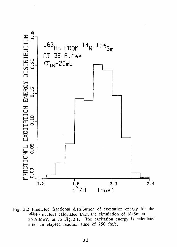
Suppose we now take a particular nucleus close to the peak of the

fractional mass distribution in Fig. 3.1, and evaluate its average

excitation energy. We choose the l63Ho nucleus whose ground state

energy is -8.34 MeV by the QPD rnodel.l7 The fractional distribution

of excitation energy for this nucleus is shown in Fig. 3.2 where the

same integration and normalization are chosen as those in Fig. 3.1.

There is still a substantial amount of excitation energy remaining in

the residual system. The excitation energy of the system found in

the reaction with a larger in-medium NN cross section is higher than

that of the one with smaller oNN. Presumably, this arises because

there are more nucleon-nucleon collisions at higher ~ N N and the

system is more thermalized.

In order to study the decay of the residual nuclei in a longer elapsed

time frame, we randomly choose 100 and 70 163Ho nuclei from all

residual reaction products at oNN=28 and 60 mb respectively.

Quasiparticles of each residual nucleus are propagated for another

1000 fmlc. It takes about 15 cpu-minutes to execute one event.

We find that 12 out of 100 (12%) residual nuclei produced with

oNN=28 mb undergo further decay by emitting one neutron. The

rate for those at oNN=60 mb is 16 out of 70 (23%). We expect that

the nuclei produced with oNN=60 mb will eventually emit more

particles than those at oNN=28 mb if we allow the simulation to

continue to 30,000 fm/c=lO-l9 second, which is the time scale of

evaporative decay. In other words, the masses of the residual nuclei

at oNN=60 mb will be less than those at oNN=28 mb. We have not

performed the 30,000 fm/c calculation because it takes over 6 cpu-

hours to execute one event. Even if we were to do so, the system

may still be excited because (i) the QPD model is a classical model

and does not include any decay via tunnelling through the potential

barrier; and (ii) the model does not include any decay via the

emission of gamma rays for which the time scale is in the order of

1 0-16 second.

Finally, we briefly discuss the systematic errors associated with the

QPD code. The errors are associated with non-conservation of linear

and angular momentum due to the finite step size of the equation of

motion integration routine. The change in energy for a cluster is in

the order of 0.1 MeV/A over an elapsed time of 250 fmlc.17 The

change of angular momentum is observed to be less than 1% over an

elapsed time of 1000 fmlc. Therefore, the QPD code conserves both

energy and angular momentum very well; the main source of error

in our predictions is statistical.

150 153 156 159 162 165 168

MASS

Fig 3.1 Predicted heavy nucleus mass yields for N+Sm at 35 A.MeV, averaged over impact parameter and integrated over fragment energy and angle. The yields are calculated after an elapsed time of 250 fm/c. The distribution is normalized to unity over the fragment mass range shown.

1 6 3 ~ o FROM 14*+154 Sm

2.0

[ MeV I

Fig. 3.2 Predicted fractional distribution of excitation energy for the 163H0 nucleus calculated from the simulation of N+Sm at 35 A.MeV, as in Fig. 3.1. The excitation energy is calculated after an elapsed reaction time of 250 fmlc.

3.4 Single Particle Inclusive Spectra for Light Particles

As we have discussed in Chapter One, one of the features of

intermediate energy heavy-ion collisions is nonequilibrium particle

emission during the equilibration stages of the reaction. These

particles can carry kinetic energy per nucleon on the order of that of

the projectile. On the other hand, the energy carried by particles

emitted from a long-time evaporative decay is usually low. Since we

stop the reaction at 250 fm/c which is approximately equal to 10-21

second, we assume that products observed in the simulation are

predominantly via nonequilibrium emission.

In order to see how well the computer simulation agrees with the

experiment, we compare the single particle inclusive measurements

of the experiment with the predictions of the simulation. In the

experiment,lg light particles-protons, deuterons, tritons and alpha

particles-are detected at polar angles of 8=30•‹ and 60" with respect

to the momentum vector of the projectile. Because of our limited

statistics, we bin the QPD results into 20" bins centered at 30" and

60" with respect to the beam momentum vector. The differential

cross section at (E,8) is defined as:

where AE=lO MeV;

N(b) is the number of particles emitted in ASZ and within 1

(EqAE) for reaction at b;

A(b) = 10 a[(b+0.5)2 - (b-0.5)2] mb;

NT(b) is the number of events generated at b.

The proton spectra for emission at 30" and 60" are shown in Figs. 3.3

and 3.4 respectively. The results predicted by the QPD model are

indicated by histograms: the dashed curve is for oNN=28 mb, and the

solid curve is for oNN=60 mb. The experimental data are shown as

solid dots. Since the systematic errors in the propagation code are

much less than those of the statistical errors, only statistical errors of

the predicted spectra are included in Figs 3.3 to 3.8. (All the error

bars of the data and some of those of the predicted spectra for Figs.

3.3 to 3.8 are omitted because they are too small). The predicted

spectra show the usual behavior: there is a roughly exponential fall-

off with emission energy at fixed angle, and a decrease with angle at

fixed energy in the laboratory frame. The spectra for the two in-

medium NN cross sections at 60" give similar results, while at 30•‹,

the larger in-medium cross section yields a smaller inclusive cross

section at proton energies of the order of the beam energy per

nucleon.

The calculated and measured inclusive spectra for deuteron clusters

at both 30" and 60" are shown in Figs. 3.5 and 3.6 respectively.

Although the multiplicities of deuterons are about 20% of the proton

multiplicities at any specific ~ N N , angle and energy, the deuteron

spectra have similar general behavior as the proton spectra.

Deuterons from reactions with smaller ONN correspond to the larger

inclusive cross section at forward angles and fragment kinetic energy

per nucleon of the order of the beam energy per nucleon. The

agreement between the experiment and predictions is at the two I standard deviation level for deuteron fragments with kinetic energy

more than 40 MeV at both angles at oNNZ28mb.

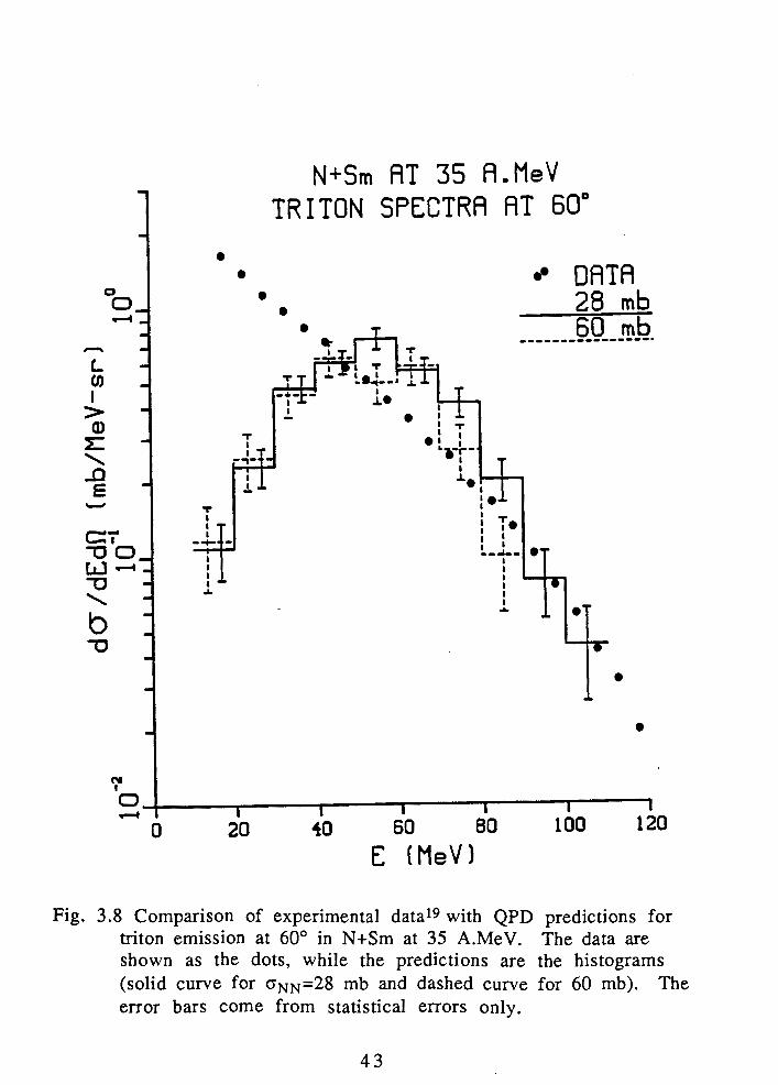
The inclusive spectra of triton clusters at both 30" and 60" are shown

in Figs. 3.7 and 3.8 respectively. The multiplicities of tritons are only

5% of the proton multiplicities at any specific ONN, angle and energy.

The exponential fall-off with the emission energy of the calculated

triton spectra is not as obvious as the proton and deuteron spectra.

The shape of both predicted triton spectra at low trigger energy is

quite different from that of the data. The agreement is quite good at

the high energy part. The agreement between the experiment and

the prediction is at the three standard deviation level for triton

fragments over 100 MeV at 30" and within two standard deviations

at 60' for those tritons with over 60 MeV at both BNN. The results of

alpha-particle clusters are not plotted because the statistics of alpha

particle production are poor.

The proton and deuteron spectra at forward angles in Figs. 3.3 and

3.5 show that the reactions at smaller ONN give larger inclusive cross

sections for both triggers at fragment kinetic energies per nucleon

larger than the projectile kinetic energy per nucleon. One may have

expected that the higher the in-medium NN cross section of the

reaction, the higher the single-particle differential cross sections. For

example, in simulations of zero impact parameter La+La collisions at

250 A.MeV, the wide angle cross section increases with in-medium

cross section. The magnitude of the increase depends on target and

projectile mass: the effect is much less pronounced for Ag+Ag than

for La+La.23

The results from Fig. 3.3 and 3.5 may appear to be somewhat

surprising, taken at face value. What appears to be happening is that

the higher the in-medium NN cross section, the greater the number

of nucleon-nucleon scatterings. The population of nucleons with

kinetic energy in the range of the projectile kinetic energy per

nucleon is being reduced by scattering. These nucleons are trapped

in excited residual nuclei which have not decayed by the time at

which the simulation is stopped. Therefore, the number of fragments

emitted at fragment kinetic energies per nucleon in the range of the

beam decreases with increasing in-medium NN cross section. On the

other hand, the energy-integrated angular distributions do not show

a particularly strong dependence on the in-medium NN cross section.

This can be seen from Table 3.1, in which the differential cross

sections for proton, deuteron, triton and alpha-particle emission are

integrated to give a fragment differential multiplicity as function of

angle. Results are shown for both oNN=28 and 60 mb.

1 60" 6 0 I 0.19 0.044 0.01 8 0.011 1 Table 3.1 : Differential multiplicities of the fragments at different

Angle GNN (mb) 30" 2 8 30" 6 0 ,

combinations of emission angle and in-medium NN cross section.

Fragment Species (dN/dQ)

P d t a 0.44 0.097 0.020 0.015 0.41 0.089 0.014 0.01 1

The results of the inclusive spectra for protons and deuterons are

generally within a factor of 2 of the experimental measurement. As

we have discussed in the last section, the excitation energy of the

residue is about 2 A.MeV. There should be more decays of the

system such as evaporative decay and gamma ray emission in a

longer time scale. Since there is no long-time evaporative decay

process built into the QPD rnodel,l7 one should be not surprised that

the predicted spectra are less than the measured spectra. Since the

energy of particles evaporated from heavy residue deexcitation is

lower than that of nonequilibrium particles from incomplete fusion

reactions, the predicted spectra (especially the low energy part of the

spectra) should be higher if evaporation of the excited residual

nucleus is considered. Moreover, the masses of the residual nuclei

should be smaller after decay. Although the predictions of the

reactions at oNN=28 mb appear to have a better agreement with the

experimental data, the experimental data do not necessarily

distinguish between either value of ~ N N , since the predictions may be

changed by long-time-frame decays.

3 PROTON SPECTRA AT 30'

g. 3.3 Comparison of experimental data19 with QPD predictions for proton emission at 30' in N+Sm at 35 A.MeV. The data are shown as the dots, while the predictions are the histograms (solid curve for oNN=28 mb and dashed curve for 60 mb). The error bars come from statistical errors only.

PROTON SPECTRA AT 60"

DATA ZtJ rnb 68 mb

Fig. 3.4 Comparison of experimental data19 with QPD predictions for proton emission at 60' in N+Sm at 35 A.MeV. The data are shown as the dots, while the predictions are the histograms (solid curve for aNN=28 mb and dashed curve for 60 mb). The error bars come from statistical errors only.

DEUTERON SPECTRA AT 30"

DATA 28 mb 60 mb .................................

Fig. 3.5 Comparison of experimental data19 with QPD predictions for deuteron emission at 30' in N+Sm at 35 A.MeV. The data are shown as the dots, while the predictions are the histograms (solid curve for oNN=28 mb and dashed curve for 60 mb). The error bars come from statistical errors only.

DEUTERON SPECTRA AT 60'

Fig. 3.6 Comparison of experimental data19 with QPD predictions for deuteron emission at 60' in N+Sm at 35 A.MeV. The data are shown as the dots, while the predictions are the histograms (solid curve for oNN=28 mb and dashed curve for 60 mb). The error bars come from statistical errors only.

N+Sm AT 35 A.MeV T R I T O N SPECTRA AT 30'

DATA

E [MeV)

Fig. 3.7 Comparison of experimental data19 with QPD predictions for triton emission at 30' in N+Sm at 35 A.MeV. The data are shown as the dots, while the predictions are the histograms (solid curve for oNN=28 mb and dashed curve for 60 mb). The error bars come from statistical errors only.

TRITON SPECTRA AT 60"

DATA

E (MeV)

Fig. 3.8 Comparison of experimental data19 with QPD predictions for triton emission at 60' in N+Sm at 35 A.MeV. The data are shown as the dots, while the predictions are the histograms (solid curve for oNN=28 mb and dashed curve for 60 mb). The error bars come from statistical errors only.

3.5 Comparison Between QPD and BUU Calculations

It is worthwhile to compare the results calculated from the QPD

model with those found in a BUU calculation.22 When we compare

the single particle inclusive spectra from the QPD simulation with

those from the BUU calculations, certain rearrangements of the QPD

results should be made. BUU calculations do not give the free

nucleon spectrum directly: an assumption has to be made in the BUU

model to extract it from the one-body distribution of nucleons in

phase space. A commonly adopted procedure is to evaluate the local

coordinate space density in a region to determine the strength of the

nuclear mean field, and from this extract the fraction of nucleons in

that region which are unbound.

In Ref. 22, a calculation of the same heavy ion reaction is performed

in the BUU model for an elapsed reaction time of 200 fm/c. In the

analysis of the simulation, individual nucleons are assumed to be

contained in a fragment if the sum of their kinetic energy and the

local U(p) which they experience is less than 6 MeV where

U(p) = -356 - + 303 - MeV; (3 (;',T and p is the local density. Otherwise nucleons are assumed to be

unbound. Under this condition, the fast unbound nucleons and the

bound residues are clearly separated. BUU predicts that the target-

like residual nuclei have mass of approximately 150 nucleons and

will continue to decrease in mass with increasing elapsed time of the

calculation due to compound evaporation processes. The average

mass of the residual nuclei calculated here by the QPD model is

approximately 10 mass units heavier than that found by the BUU

model. However, a 'cold' nucleus in its ground state can evaporate

nucleons on the time scale of a few hundred fmlc in a BUU

calculation.13 Hence, it is not certain whether the evaporation

predicted by the BUU model is due to the numerical instability of the

model or to a good approximation of the evaporation process.

In order to more directly compare our predictions with the BUU

calculation, the proton and neutron cross sections from the QPD

simulation are summed up. The spectra for mass A=l at 30" and 60"

are shown in Figs. 3.9 and 3.10 respectively. The BUU results for the

nucleon cross section are calculated with in-medium NN cross section

at 20 and 41 mb. (Some error bars for both figures are omitted

because they are too small.) The spectra from the results of the two

models are similar in shape. The spectra from the BUU calculation

are at a factor of two-three higher in magnitude than those from the

QPD simulation. The reasons for the difference may be: (i) there is

still substantial excitation energy in the residual nuclei at the time

when the QPD simulation is stopped; and (ii) the QPD spectra do not '

include the light particles with mass A>1 whereas the BUU spectra

include all nucleons which are not bound within the residual nuclei.

Given the different definition of the observables in the two models,

the agreement is in the range expected. Lastly, the BUU results for

the integrated nucleon cross section do not show strong sensitivity to

CJNN in the 20-41 mb range, which is similar to what is found in the

QPD model.

NUCLEON SPECTRA AT 30'

BUU 20 mb 0 BUU 41 mb

QPD 28 mb QPD 60 mb ........................

E [MeV)

Fig. 3.9 Comparison of BUU22 calculations with QPD predictions for nucleon emission at 30' in N+Sm at 35 A.MeV. The BUU results are shown as squares (solid square for oNN=20 mb and hollow square for 41 mb), while the QPD predictions are the histograms (solid curve for oNN=28 mb and dashed curve for 60 mb). The error bars of the QPD predictions come from statistical errors only.

NUCLEON SPECTRA AT 60"

BUU 20 mb a BUU 4 1 mb

QPD 28 mb OPD 60 mb ........................

Fig. 3.10 Comparison of BUU22 calculations with QPD predictions for nucleon emission at 60' in N+Sm at 35 A.MeV. The BUU results are showe as squares (solid square for oNN=20 mb and hollow square for 41 mb), while the QPD predictions are the histograms (solid curve for oNN=28 mb and dashed curve for 60 mb). The error bars of the QPD predictions come from statistical errors only.

Chapter Four

Gamma Ray Circular Polarization

4.1 Introduction

In the last chapter, we showed that the single particle inclusive

spectra predicted by the QPD model give reasonable agreement with

experiment. However, such comparisons reveal little of the

relationship between the reaction dynamics and the nonequilibrium

particles emitted. Nor do they show any azimuthal anisotropies of

the light particles emitted. For example, one question of interest is

the correlation between the trigger plane and the reaction plane.

Such effects can only be revealed by more complex coincidence

measurements.

The first experimental evidence that nonequilibrium light particle

emission from fusion-like reactions exhibit large azimuthal

asymmetries was obtained from 14N induced reactions on 197Au at

E/A=30 MeV.18 The data show that nonequilibrium light particles

are emitted preferentially in the plane perpendicular to the entrance

channel orbital angular momentum, indicating there is a collective

motion in the plane and transverse to the beam axis. Microscopic

calculations with the BUU equation interpret this effect in terms of a

deflection to negative emission angles by the attractive nuclear mean

field.14 However, the collective motion in the nuclear mean field is

damped by nucleon-nucleon collisions. The relative importance of

positive and negative emission angles is sensitive to the interplay

between the nuclear mean field and nucleon-nucleon collisions.

Tsang and co-workers address these issues experimentally by

determining the circular polarization of gamma rays emitted by the

residual nucleus in coincidence with the nonequilibrium light particle

emission for the reaction l4N on 154Sm at E/A = 35 MeV.19 They

observe that the gamma rays are positively circularly polarized,

which corresponds to negative deflection angles as discussed in

Chapter One. In this chapter, we use the QPD model to predict the

gamma rays' circular polarization, and to study the correlation

between the trigger plane and the reaction plane. The results are

compared with those of the experiments and those calculated with

the BUU model in Sections 4.3 and 4.4 respectively. Finally, the

microscopic dynamics of the collision process is studied in

Section 4.5.

4.2 Methodology

The measurements of the circular polarization of gamma rays

emitted by the residual nuclei in coincidence with the emission of

light particle triggers are performed at the National Superconducting

Cyclotron Laboratory of Michigan State University.19 The method of

detecting the light particles is described in the last chapter. The

polarimeter to measure the circular polarization of gamma rays

emitted defines a quantization axis, perpendicular to the trigger

plane. The details of the experimental set up are thoroughly

discussed in Refs. 19 and 24.

The QPD model can give information about the positions, momenta,

excitation energies and angular momenta of clusters at any time

during the reaction. It does not include any mechanism for dealing

with gamma ray emission. In order to calculate the circular

polarization of the gamma rays, we adopt a model advanced in

Ref. 19 in which the spin deexcitation of the heavy residual nucleus

is assumed to proceed via stretched E2 transitions. Such transitions

have a gamma ray multiplicity of M=IJ1/2 for a residual nucleus with

angular momentum J. In the calculation, we only consider the orbital

angular momentum of the nucleus and ignore the intrinsic spin of the

nucleons.

Before we go on any further, let us discuss the labelling convention

for the vectors involved in the circular polarization calculation, as

shown in Figure 4.1. The momenta of the beam, ki, and the trigger

fragment, k f , are used to define a trigger plane. The quantization k ixkf

axis Bif is defined by I - irlkixkfl

at which the polarimeter is located.

The initial reaction plane, defined by the beam direction and the

impact parameter vector b lies at an angle $ with respect to the

trigger plane.

Reaction 7 Fig. 4.1 Sign convention for vectors and planes involved in the

circular polarization determination. The vector J is the orbital angular momentum of the residual nucleus. The momentum vector of the beam k i and that of the trigger kf form the trigger plane. The impact parameter vector b and k i form the reaction plane.

For each simulation event, there is only one large residual nucleus

present, and its angular momentum vector is used to calculate the

characteristics of the emitted gamma rays. In the stretched E2

cascade, gamma rays with momentum k are emitted from the

residual nucleus with an angular distribution,

whe re

The circular polarization of gamma ray is then:

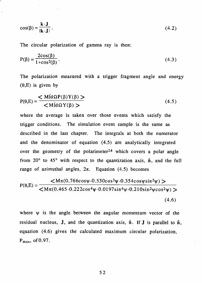
The polarization measured with a trigger fragment angle and energy

(8,E) is given by

where the average is taken over those events which satisfy the

trigger conditions. The simulation event sample is the same as

described in the last chapter. The integrals at both the numerator

and the denominator of equation (4.5) are analytically integrated

over the geometry of the polarimeter24 which covers a polar angle

from 20" to 45" with respect to the quantization axis, ii, and the full

range of azimuthal angles, 27c. Equation (4.5) becomes

where yr is the angle between the angular momentum vector of the

residual nucleus, J , and the quantization axis, ii. If J is parallel to ii,

equation (4.6) gives the calculated maximum circular polarization,

P,,,, of 0.97.

If we write Eq. 4.6 as

then the statistical errors for the circular polarization are

4.3 Results of the Calculation

We begin with an overview of the behavior of the calculated circular

polarization. In Figure 4.2, we show the dependence of the predicted

polarization on fragment trigger mass and kinetic energy. (Since the

systematical errors which are arrived from the uncertainties of the

conservation of angular momentum are much less than the statistical

errors, only statistical errors are included in all predicted circular

polarization plots from Figs. 4.2 to 4.8). The trigger angle is fixed at

30' and the in-medium NN cross section is chosen as 28 mb. Positive

circular polarizations are observed for all trigger masses and kinetic

energies. There are two trends: the circular polarization increases

with the trigger mass and kinetic energy. These trends are

qualitatively similar to what is observed experimentally.

The dependence of trigger angle and kinetic energy for protons and

deuterons (both at oNN=28 mb) are shown at Figures 4.3 and 4.4

respectively. For proton triggers, there is little difference in the

circular polarization calculated at 30" and at 60". For deuteron

triggers, the angular dependence is more pronounced: the circular

polarization increases with trigger angle. The trigger energy

dependence shows a similar trend for both trigger fragment masses

at both angles: circular polarization increases with trigger energy.

These observations qualitatively agree with what is measured

experimentally. We do not calculate the circular polarization at

wider angles for either trigger fragments because we do not have

enough statistics to draw any conclusion.

Figures 4.5 and 4.6 show the calculated circular polarization at two

in-medium NN cross sections and the experimentally measured one

for proton triggers at 30" and at 60" respectively. It is obvious that

the circular polarization predicted by the computer simulation

decreases with increasing in-medium NN cross section. This is

because more nucleon-nucleon collisions in the reaction with larger

in-medium NN cross section tend to reduce the angular momentum

alignment of the residual nucleus. The effect of decreasing circular

polarization with increasing QNN is also seen in deuteron and triton

triggers. Figures 4.7 and 4.8 show the results of the deuteron

triggers.

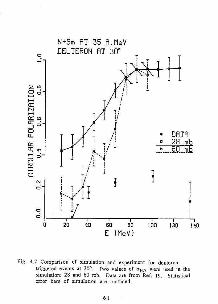
As shown in Figs. 4.5 to 4.8, the calculated circular polarizations are

much higher than the measured ones. In Fig. 4.5, the calculated and

the measured circular polarizations for proton triggers at energy

below 40 MeV at 30' in oNN=60mb disagree by several standard

deviations. The agreement for deuteron triggers at low energies at

30" and oNN=60mb is within their uncertainty ranges but the errors

are large. There are two reasons to explain the discrepancy between

our predictions and the data:

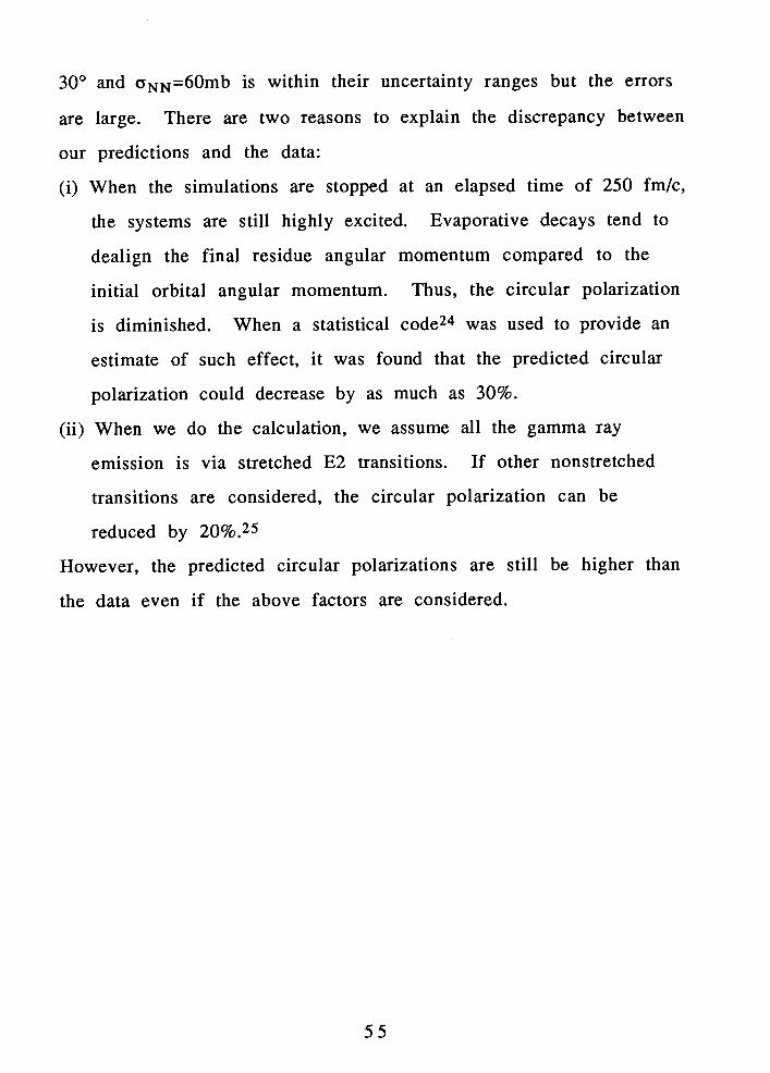
(i) When the simulations are stopped at an elapsed time of 250 fm/c,

the systems are still highly excited. Evaporative decays tend to

dealign the final residue angular momentum compared to the

initial orbital angular momentum. Thus, the circular polarization

is diminished. When a statistical code24 was used to provide an

estimate of such effect, it was found that the predicted circular

polarization could decrease by as much as 30%.

(ii) When we do the calculation, we assume all the gamma ray

emission is via stretched E2 transitions. If other nonstretched

transitions are considered, the circular polarization can be

reduced by 2O%.25

However, the predicted circular polarizations are still be higher than

the data even if the above factors are considered.

KINETIC ENERGY (MeV)

Fig. 4.2 Predicted trigger mass and energy dependence of circular polarization observed at 30'. An in-medium NN cross section of 28 mb is used for the calculation. The results are for the reaction N+Sm at 35 A.MeV and are averaged over impact parameter. Selected statistical error bars are included.

N+Sm AT 35 A.MeV PROTON AT DNN-28mb

E [MeV)

Fig. 4.3 Predicted proton trigger emission energy dependence of circular polarization shown at both 30" and 60'. Other conditions are as in Fig. 4.2. Statistical error bars are included.

Fig. 4.4 Predicted deuteron trigger emission energy dependence of circular polarization shown at both 30' and 60'. Other conditions are as in Fig. 4.2. Statistical error bars are included.

Fig. 4.5 Comparison of simulation and experiment for proton triggered events at 30'. Two values of GNN were used in the simulation: 28 and 60 mb. Data are from Ref. 19. Statistical error bars of simulation are included.

DATA

Fig. 4.6 Comparison of simulation and experiment for proton triggered events at 60'. Two values of CJNN were used in the simulation: 28 and 60 mb. Data are from Ref. 19. Statistical error bars of simulations are included.

N+Sm AT 35 A.MeV DEUTERON AT 30"

DATA

Fig. 4.7 Comparison of simulation and experiment for deuteron triggered events at 30'. Two values of ~ N N were used in the simulation: 28 and 60 mb. Data are from Ref. 19. Statistical error bars of simulation are included.

N+Sm RT 35 R.MeV DEUTERON RT 60"

1 T

DRTR

60

[ MeV I

Fig. 4.8 Comparison of simulation and experiment for deuteron triggered events at 60'. Two values of GNN were used in the simulation: 28 and 60 mb. Data are from Ref. 19. Statistical error bars of simulation are included.

4.4 Comparison with BUU Calculations

Since the circular polarization experiment has been analyzed through

the BUU model, it is worthwhile making a comparison between the

QPD predictions and those obtained in a BUU calculation19 of the

same reaction. As we have mentioned in the last chapter, the BUU

code separates the fast 'unbound' nucleons from the bound target-

like nuclei. It cannot distinguish different species of fragments. The

results calculated with the BUU simulation in Ref. 19 are energy

integrated. In order to compare our results with those of the

simulation in Ref. 19, we calculate the circular polarization

associated with a single nucleon trigger averaged over trigger

energy. The results of both QPD and BUU models are shown in Table

4.1. The results predicted by QPD are higher than those by the BUU

model by about 50% for a similar ONN.

Table 4.1 Gamma ray circular polarization associated with nucleon triggers predicted by the QPD and BUU models. Results of the BUU model are taken from Ref. 19.

Model

QpD II

BUU

QpD It

BUU

ONN (mb) 2 8 6 0 4 1

2 8 6 0 4 1

8

30" II

I t

60" 11

I1

P

0.38 0.24 0.18

0.5 1 0.40 0.25

In order to illustrate the dependence of the predicted circular

polarizations on the nucleon-nucleon collision dynamics, the BUU

model19 is used to calculate the circular polarizations using various

nucleon-nucleon scattering cross sections at a fixed impact parameter

b = 6.5 fm. The results are shown in Table 4.2. The predicted

circular polarizations decrease for larger values of ONN. These results

qualitatively agree with our results: the reactions with larger oNN

give smaller circular polarizations.

Table 4.2 Circular polarization predicted19 by the BUU model using different ONN at a fixed impact parameter of b = 6.5 fm. The nucleon trigger angle is 60'.

4.5 Microscopic Dynamics of the Collision Process

Let us now use the results of the computer simulations to examine

the microscopic dynamics of the collision process. The simulation has

predicted large values for the circular polarization of the gamma rays

emitted. Thus, one expects that there is a strong correlation between

the trigger plane and the reaction plane. We begin our investigation

of this question by examining the distributions of the impact

parameters for a given trigger energy and angle. In this section, let

us use the x and z axes of a Cartesian coordinate system to define the

trigger plane: the z-axis is defined by the beam direction and the

positive x-axis is the direction in which lies that component of the

trigger momentum which is perpendicular to the beam. The impact

parameter vector then lies in the x-y plane perpendicular to the

beam.

A scatter plot (from the simulation) of the impact parameter for

proton triggers at 30' with 28 mb for the in-medium NN cross

section is plotted in Figure 4.9. The three sections of the plot

correspond to proton kinetic energies of 20-30, 40-50 and 60-70

MeV respectively. Each dot on the plots represents the point where

the beam intersects the x-y plane for one event. In other words, the

impact parameter vector for each event is from the origin to the dot.

In generating the scatter plots, we have shifted the magnitude (but

not the direction) of the impact vector randomly up to k0.5 fm. If

the magnitudes are not shifted, the data points will fall in concentric

circles because the impact parameters used in the simulation are

taken to be 0.5, 1.5, ... , 7.5 fm in 1 fm steps. The shift of magnitude

will give a more clear display of the density of points.

At low proton trigger energy, there is a very pronounced

enhancement for impact parameters on the opposite side of the beam

from the trigger momentum. There is a small enhancement on the

same side as the trigger momentum. As one compares parts a) to c)

of Figure 4.9, one can see the tendency for the impact parameter to

be located on the opposite side of the trigger momentum becoming

stronger with trigger energy. The same behavior can be found in the

scatter plots of the deuteron trigger. Figure 4.10 shows the deuteron

trigger at kinetic energies of 20-30, 40-50, 60-70 and 80-90 MeV

respectively. The conditions are same as those in Figure 4.9. We can

conclude that the higher the trigger energy, the stronger the

tendency to scatter to the opposite side of the impact parameter

vector, i.e., the stronger the tendency of negative deflection.

For both trigger masses, the results of the simulation show that the

path of the beam nucleus is bent around the target nucleus as the

two nuclei interact. Some of the mass of the projectile is transferred

to the target nucleus which gains angular momentum. The projectile

nucleus usually does not "bounce off" the target, i.e. be positively

deflected, at these trigger energies. This tendency is also what we

have been led to expect from the circular polarization results.

To make a more quantitative argument, we evaluate the expectation

value of the angle @ between the reaction plane and the trigger plane.

For all the cases considered, $=(@) is close to n, as one would expect.

However, the average of randomly distributed angles on a plane is

also n. To make sure the @ is not randomly distributed, we have

evaluated the dispersion D of the angle @ where the dispersion D is

defined as ( ( @ - ~ ) ~ ) l / ~ . For randomly distributed angles on a plane,

the dispersion is equal to n / G . The calculated relative dispersion D

R = - ~ 1 4 3 ' is observed to decrease with increasing trigger energy

and, correspondingly, with circular polarization. Figure 4.11 shows

the behavior of the relative dispersion as a function of the circular

polarization for proton and deuteron triggers at 30' and oNN=28 mb.

This figure is constructed by evaluating the dispersion and the

circular polarization for each energy bin in Figures 4.6 and 4.8.

For low values of the circular polarization, the relative dispersion

tends towards unity, indicating a random distribution of impact

parameters on the xy-plane. As the circular polarization increases,

the width of the impact parameter distribution narrows and the

relative dispersion tends to zero as the circular polarization

approaches unity. This is what one would expect: the larger the

circular polarization (i.e., the more the angular momentum vector of

the residual nucleus is perpendicular to the reaction plane), the more

the reaction and trigger planes are coincident. In other words, the

simulation shows the circular polarization is a good indicator of the

correlation between the reaction and trigger planes.

PROTONS FROM N + Sm AT 35 A*MeV e=30•‹, a,, =28rnb

(a) 25 MeV (b) 45 MeV

(c) 65 MeV

Fig. 4.9 Distribution of impact parameter b for proton triggers emitted at 30' and a range of energies. The acceptance range of each energy shown is +5 MeV. Cross marks are placed on the axes every 4 fm.

DEUTERONS FROM N + Sm AT 35 A o M e V

8=30•‹, ONN =28mb

(a) 25 M e V (b) 45 M e V

(c) 65 M e V (d) 85 MeV

Fig. 4.10 Distribution of impact parameter b for deuteron triggers emitted at 30'.

o - PROTON - DEUTERON

0.4 0.6 0.8

CIRCULRR POLARIZATlON

Fig. 4.11 Relative dispersion of the orientation of the reaction plane with respect to the trigger plane shown as a function of circular polarization for both values of CTNN in the simulation.

Chapter Five

Conc lus ion

In this thesis, we perform a computer simulation based on the QPD

model for the reaction of 14N+l54Sm at 35 A.MeV. The single particle

- proton, deuteron and triton - inclusive spectra and the gamma ray

circular polarization in coincident with the light particle triggers are

studied. The results are compared with the experimentally observed

values and those calculated from the BUU model.

The' difference between the data and the QPD are usually within

three standard deviations for the inclusive spectra. The agreement is

in the range expected. The difference between A value of 28 mb

chosen for the in-medium NN cross section gives better agreement

with the data compared to 60 mb, but a solid conclusion cannot be

drawn because of the uncertainties which may arise from effects

which are not incorporated in the model.

For example, the collision is only followed for a time of 250 fm/c

which is long enough to ensure that the clusters are stabilized. The

residual system is still highly excited. It takes a much longer time

for the residues and other clusters to decay into their ground states

by particle or gamma emission- fiocesses such as evaporation have

a much longer time-scale than that for which it is practicable to run

the simulation. Moreover, the QPD model does not include any decay

via tunnelling through the potentid b d e r nor a mechanism for

dealing with gamma decay. It is impossible for the QPD model to

predict long-time decay. Certainly, long-time-frame evaporation will

boost the yields of light mass particles and might bring the

oNN=60 mb predictions into better agreement with the data.

The nucleon spectra calculated from the QPD model have a similar

shape to those found in a BUU calculation. The spectra from the BUU

model are at a factor of two-three higher in magnitude than those

from the QPD model. Given the different definition of the observable

in the two models, the agreement is in the range expected.

The predicted circular polarizations are in qualitative agreement

with the data in terms of trends with respect to fragment trigger,

mass, energy and emission angle. However, the predictions by the

QPD model are consistently higher than the data. Again, part of the

reason for the discrepancy lies in long-time decays which will reduce

the alignment of the angular momentum vector of the residual

nucleus.

To see how large an effect this would be on the time scale of

1000 fm/c, we take a sample of the 163Ho nuclei discussed in

Chapter Three and propagate them for an extra 1000 fm/c. The

change in orientation of the angular momentum vector is observed to

be less than 1%. This demonstrates:

i) that there are few evaporative decays on a time frame which can

be handled by the simulation, and

ii) that the simulation conserves angular momentum very well.

When a statistical decay code was used24 to provide an estimate of

the depolarization effects of evaporative decays, it was found that

the predicted circular polarization could decrease by as much as 30%.

This estimate significantly reduces the discrepancy between our

predictions and the data, but does not eliminate it entirely. Lastly

the assumption that the gamma decays are stretched E2 may be too

strong. If other nonstretched transitions are considered, the circular

polarization can be reduced by 20%.25

The circular polarizations calculated from the BUU model, which are

about 50% of those predicted by the QPD model, seem to give better

agreement with the data in comparison with the results of the QPD

model. However, individual nucleon-nucleon scattering in the BUU

model19 that we are comparing with does not necessarily conserve

angular momentum. (The observed angular momentum for the

whole nuclear system is usually conserved). On the other hand, the

angular momentum of nucleon-nucleon scattering and thus that of

the whole nuclear system in the QPD model is conserved. Since the

conservation of angular momentum is a very important factor in the

determination of the gamma ray circular polarization, we cannot

agree that the BUU model gives better prediction than the QPD does.

The central question which we ask of the simulation is whether there

is a strong correlation between the circular polarization and the

distribution of the reaction plane's orientation with respect to the

trigger plane. The simulation finds that the angle between the two

planes is about 180' and the dispersion of the angle decreases as the

circular polarization increases. Therefore, it shows that there is

indeed a correlation, and that the correlation becomes stronger the

closer the circular polarization is to unity. Further the impact

parameter tends to point in the opposite direction to the trigger

direction. This indicates that the long range nuclear interaction tends

to pull the nuclei around one another, although not sufficiently

strongly as to result in an orbiting pair at these bombarding energies.

References:

Bertsch, G.F., and S. Das Gupta, Physics Reports 160, 189 (1 988).

Gelbke, C.K., and D.H. Boal, Prog. Part. Nucl. Phys. 19, 33 (1987).

Stocker, H., and W. Greiner, Physics Reports 137, 277 (1 986).

Boal, D.H., Ann. Rev. Nucl. Part. Sci. 37, 1 (1987).

Kikuchi, K., and M. Kawai, Nuclear Matter and Nuclear Reaction . (North-Holland: Amsterdam, 1968).

Nix, J.R., et al, Phys. Rev. C25, 2491 (1982).

Cugnon, J., Lecture given a t Cargese Summer School (1984).

Bertsch, G., and J. Cugnon, Phys. Rev. C24, 2514 (1981).

Balescu, R., Equilibrium and Nonequilibrium Statistical Mechanics. (Wiley: New York, 1975).

Nordheim, L.W., Proc. R. Soc. London, Ser. A 119, 689 (1928).

Uehling, E.A., and G.E. Uhlenbeck, Phys. Rev. 43, 552 (1933).

Binder, K., Application of the Monte Carlo Method in Statistical Physics. (Springer-Verlag: New York, 1987).

Gan, H.H., S.J. Lee and S. Das Gupta, Phys. Rev. C36, 2365 (1987).

Aichelin, J., and G. Bertsch, Phys. Rev. C31, 1730 (1985).

Kruse, H., et al, Phys. Rev. C31, 1770 (1985).

For example, see C. Gale and S. Das Gupta, Phys. Lett. 162B, 35 (1985); G.E. Beauvais et al, Phys. Rev. C35, 545 (1987); J. Aichelin and H. Stocker, Phys. Lett. 176B, 14 (1986).

Boal, D.H., and J.N. Glosli, Phys. Rev. C38, 1870 (1988); and Phys. Rev. C38, 2621 (1988).

Tsang, M.B., et al., Phys. Rev. Lett. 52, 1967 (1984).

1 9 Tsang, M.B., et al., Phys. Rev. Lett. 57, 559 (1986).

2 0 Trautmann, W., et al., Phys Rev. Lett. 53, 1630 (1984).

2 1 Bertsch, G.F., H. Kruse and S. Das Gupta, Phys. Rev. C 29, 673 (1984).

2 2 Tsang, M.B., et al., Michigan State University Preprint: MSUCL- 681.

2 3 Boal, D.H., private communication.

2 4 Trautmann, W., et al., Nucl. Instrum. Methods 184, 449 (1981).

2 5 Trautmann, W., et al., Nucl. Phys. A422, 418 (1984).