a concept of bayesian regulation in fisheries management

A Concept of Bayesian Regulation in FisheriesManagementNoel Michael Andre Holmgren1*, Niclas Norrstrom1, Robert Aps2, Sakari Kuikka3

1 Systems Biology Research Centre, School of Bioscience, University of Skovde, Skovde, Sweden, 2 University of Tartu, Estonian Marine Institute, Tallinn, Estonia, 3 Fisheries

and Environmental Management Group, Department of Environmental Sciences, University of Helsinki, Helsinki, Finland

Abstract

Stochastic variability of biological processes and uncertainty of stock properties compel fisheries managers to look for toolsto improve control over the stock. Inspired by animals exploiting hidden prey, we have taken a biomimetic approachcombining catch and effort in a concept of Bayesian regulation (BR). The BR provides a real-time Bayesian stock estimate,and can operate without separate stock assessment. We compared the performance of BR with catch-only regulation (CR),alternatively operating with N-target (the stock size giving maximum sustainable yield, MSY) and F-target (the fishingmortality giving MSY) on a stock model of Baltic Sea herring. N-targeted BR gave 3% higher yields than F-targeted BR andCR, and 7% higher yields than N-targeted CR. The BRs reduced coefficient of variance (CV) in fishing mortality compared toCR by 99.6% (from 25.2 to 0.1) when operated with F-target, and by about 80% (from 158.4 to 68.4/70.1 depending on howthe prior is set) in stock size when operated with N-target. Even though F-targeted fishery reduced CV in pre-harvest stocksize by 19–22%, it increased the dominant period length of population fluctuations from 20 to 60–80 years. In contrast, N-targeted BR made the periodic variation more similar to white noise. We discuss the conditions when BRs can be suitabletools to achieve sustainable yields while minimizing undesirable fluctuations in stock size or fishing effort.

Citation: Holmgren NMA, Norrstrom N, Aps R, Kuikka S (2014) A Concept of Bayesian Regulation in Fisheries Management. PLoS ONE 9(11): e111614. doi:10.1371/journal.pone.0111614

Editor: Jeffrey Buckel, North Carolina State University, United States of America

Received March 26, 2014; Accepted October 2, 2014; Published November 3, 2014

Copyright: � 2014 Holmgren et al. This is an open-access article distributed under the terms of the Creative Commons Attribution License, which permitsunrestricted use, distribution, and reproduction in any medium, provided the original author and source are credited.

Data Availability: Data presented in this paper are from a third party (ICES) which has published the data in a report (ICES (2009) Report of the Baltic FisheriesAssessment Working Group (WGBFAS), 22 - 28 April 2009, ICES Headquarters, Copenhagen. ICES CM 2009\ACOM:07. 626 pp). The data is publicly available intables of this report: http://www.ices.dk/sites/pub/Publication%20Reports/Expert%20Group%20Report/acom/2009/WGBFAS/WGBFAS09.pdf. The results fromthese simulations can now be generated by readers since the authors have provided the code as supporting information.

Funding: The study is part of the IBAM project ‘‘Integrated Bayesian risk analysis of ecosystem management – Gulf of Finland as a case study’’, which receivedfunding from the European Community’s Seventh Framework Programme under grant agreement 217246 made with the joint Baltic Sea research anddevelopment programme BONUS (http://www.bonusportal.org/), from FORMAS, Sweden, the Academy of Finland, and an Estonian Science Foundation grant7609, Estonian target financed theme SF0180104s08. The funders had no role in study design, data collection and analysis, decision to publish, or preparation ofthe manuscript.

Competing Interests: The authors have declared that no competing interests exist.

* Email: [email protected]

Introduction

Fisheries managers are challenged with two widely permeated

properties of their study system, uncertainty [1–3] and variability

[4–6]. These can confound each other, e.g. imprecise spawning

stock size estimates can generate apparent variability in the stock

2 recruitment relationship [7]. Reduced inter-annual variability

in effort has socio-economic benefits with yields matching the

capacity of the processing industry [8], a more stable job market,

and fewer years with over-dimensioned fleets [9]. Often there is a

trade-off between maximizing yield and stabilizing yield and

fishing effort that makes management objectives ambiguous [10–

12]. There are also concerns that fishing increases the temporal

variability of harvested stocks, [4,13–15].

The problem with temporal variability in fisheries has led to an

increased interest in the performance of alternative harvest control

rules [16–18]. Stephenson et al. [19] argue that the total allowable

catch (TAC) could be used to prevent unsustainable use, but is

insufficient to control spatial and temporal variability, and cannot

be used to achieve socioeconomic objectives. In a reflection over

proposed alternative harvest controls, May et al. [20] conclude

that further mathematical refinement is probably not as important

as developing ‘‘robustly self-correcting strategies that can operate

with only fuzzy knowledge about stock levels and recruitment

curves’’. If our belief of the stock size is a probability function (in

contrast to a point estimate), Bayes’ theorem postulates that

harvesting information can be used to calculate a conditional

probability function [21]. Here we propose Bayesian regulation

(BR) that uses catch- and effort data from the ongoing fisheries to

make real-time estimates of stock size and fishing mortality. The

years can be linked by using the posterior distribution as a prior in

the sequential year, and hence exploitation is combined with stock

size assessment. Real-time assessment of BR would be advanta-

geous to management routines relying on forecasts of stock

abundances. Given that most commercial fisheries with CR-based

control of biomass and fishing mortality (e.g. TAC) routinely

monitor effort and catch, this additional information is surprisingly

poorly utilized during the CR fishing season. We suggest a

methodology where this information can be used for updating

population size estimates to facilitate in-season management

decisions.

The BR is derived from Bayesian foraging theory in behavioral

ecology, which describes a giving-up rule for patch foraging

animals [22–24]. The rule is a relaxation of the full information

PLOS ONE | www.plosone.org 1 November 2014 | Volume 9 | Issue 11 | e111614

http://creativecommons.org/licenses/by/4.0/

http://www.ices.dk/sites/pub/Publication%20Reports/Expert%20Group%20Report/acom/2009/WGBFAS/WGBFAS09.pdf

http://crossmark.crossref.org/dialog/?doi=10.1371/journal.pone.0111614&domain=pdf

assumption of the marginal value theorem [25], with search time

and number of prey caught as information variables. It applies to

patches in which the prey are hidden, such as a woodpecker

feeding on pupae under bark [26,27]. Given some prior

information available to the forager, e.g. experience from foraging

in patches of its territory, a Bayesian posterior distribution can

represent the forager’s continuously changing belief about the prey

density in the current patch [28]. The animal maximizing its

intake rate would thus leave the patch for a new one when the

anticipated intake rate in the current patch drops below the one

expected from patches on average in the territory. The expected

number of remaining prey in a patch can be expressed with a fairly

simple equation derived by Iwasa et al. [29], but the decision to

leave should include a discounting of the value of further bits of

information [30].

For fisheries applications, we have modified Iwasa’s equation for

Bayesian prey density estimation for recurrent exploitation of one

population. Both are cases of Bayesian update of mean and

variance of a population size estimate. In the original scenario, the

exploiter is informed by the mean and variance of several

exploited patches within its foraging area. In the fishery scenario,

the exploiter (manager) is informed by previous exploitations and

surveys in the same area, followed by quantitative assessment and

stochastic forecast simulations. We compare CR with BR, and

show how they perform in relation to management objectives and

targets, by simulating fishing on a model of the main basin Baltic

Sea herring (Appendix S2) [31]. We present levels and temporal

variability in yield, fishing mortality, stock abundance, spawning

stock biomass (SSB), and finally how frequently it surpasses the

MSY related reference point Btrigger [32].

Methods

We look at three levels of decision-making in fisheries

management as they are described in the common fisheries policy

of the Council of the European Union [33]: (i) The managementobjective, which is the ultimate goal of fisheries management. The

objective can be simple or more complex, for example weighing

incompatible goals [34,35]. We have chosen the maximum

sustainable yield (MSY) because it is the current objective of

fisheries management in the EU [36]. (ii) The target of

Table 1. Characteristics and settings for the evaluation of eight different harvest controls: CR being a simple catch-only regulation;BR is the proposed regulation combining catch and effort.

Harvest Target Supervision Prior Prior

control m v

CRFs FMSY Supervised N+e 0

CRFu FMSY Unsupervised NMSY 0

CRNs N’MSY Supervised N+e 0

CRNu N’MSY Unsupervised NMSY 0

BRFs FMSY Supervised N+e var(NMSY)

BRFu FMSY Unsupervised NMSY var(NMSY)

BRNs N’MSY Supervised N+e var(NMSY)

BRNu N’MSY Unsupervised NMSY var(NMSY)

The subscript denotes type of target and the superscript the existence of supervision. The target column denotes the targets used: FMSY is the fishing mortality givinghighest yield in the MSY-analysis of the SOM, and N’MSY is the corresponding post-harvest stock size. The management is either supervised with a separate assessmentor unsupervised (see methods). For unsupervised management we use the mean, m, and the variance, v, of the pre-harvest stock size from MSY-analyses: NMSY. Insupervised management m is instead the actual pre-harvest stock size, N, with an added randomly generated error term e drawn from the normal distribution, (mean = 0,var = var(NMSY) where var(NMSY) is taken from an MSY-analysis).doi:10.1371/journal.pone.0111614.t001

Figure 1. (A) Bayesian regulation curves indicating the combined totalcatch (y-axis) and total effort (x-axis) when fishing should be terminatedfor the season. The curves are given by equation 1 when r is set to thetarget number of fish, and solved for total catch. Hence, the curvesshow when the fishery target is achieved in catch-effort space, given bythe ratio of variance (v) to mean stock size (m). There are four qualitativecases of the v-m ratio: when the ratio is zero, the fishery is regulated bycatch only because there is no uncertainty around the mean. When theratio equals 1, regulation is by effort only. Apart from these specialcases, the fishery should be regulated by both catch and effort. If thevariance is lower than the mean, the posterior mean will decrease withaccumulating catches and effort. If the variance is higher than themean, the posterior mean will increase with increasing catches butdecrease with effort. These effects can be deduced from analyzingequation 1. (B) Here the solid curve denotes the Bayesian regulationwhen v.m, which is determined prior to the fishing season (seeMethods). The grey curves are idealized trajectories of how cumulativecatch and effort develops from the origin during the fishing season.When the trajectories cross the regulation curve, the Bayesian posterioris on target, and the fishery should be closed for the season. Thehatched grey line indicates when the initial stock size is at the priormean (m), the solid grey line when the stock size is at the mean plus onestandard deviation (see FMSY -analysis). The BR thus allows largercatches when the stock size has been underestimated, and vice versa.doi:10.1371/journal.pone.0111614.g001

Bayesian Regulation in Fisheries Management


exploitation, which should be given in a quantitative unit that

relates to the management objective. We compare the efficiency of

two targets: fishing mortality (FMSY) and post-harvest stock size

(NMSY). (iii) The harvest rules, which ‘‘[lay] down the manner in

which annual catch and/or fishing effort limits are to be calculated

and provide for other specific management measures, taking

account also of the effect on other species’’ [33]. On this level we

choose to use other terms. We use the term regulation type to

denote the use of catch and/or effort regulation, whereas the term

harvest control rule (HCR) is used for the combined objective,

target and regulation type.

The harvest control rules under development by the Interna-

tional Council for the Exploration of the Sea (ICES) involve a

fishing mortality target (F*) and the spawning stock biomass

reference point Btrigger [32,37]. If the SSB goes below Btrigger the

fishing mortality is reduced below target, a situation that should

warrant a reinvestigation of the stock condition and the harvest

control [32]. Based on a stock assessment and a short-term

forecast, the fishing mortality target is recalculated as a TAC,

which is how the recommendation is presented to the European

Commission [38]. ICES harvest control rules use precautionary

reference points below which fishing mortality is reduced [32],

something we do not use in our simulations. We have focused on

the principle differences between CR and BR, e.g. the elaborate

data collection and assessment procedure is simplified by using the

actual size of the simulated stock with a random error.

Harvest controlAltogether we compared eight different harvest controls

achieved by the combinations of two exploitation targets, two

regulation types and two stock assessment modes (Table 1). The

Bayesian regulation BR(c, f|m, n) is a function of catch (c) and

effort (f) given the prior information of the estimated stock size

before harvest, m, and the uncertainty of that estimate given as

variance, n. The Bayesian estimate of the number of remaining

individuals (r) in a harvested stock is:

r~m{c 1{ v

m

� �

eq f {1ð Þ vm z1

ð1Þ

where q, the catchability, is defined as the fraction of the

population captured by one unit of fishing effort and is the scalar

Table 2. Mean, standard deviation and CV (%) of annual yield.

100 yrs 20,000 yrs

mean SD CV mean SD CV

CRFs 256.6 72.0 28.1 254.3 83.9 33.0

CRNs 220.3 322.4 146.3 244.5 343.0 140.3

BRFs 282.8 50.6 17.9 258.6 58.9 22.8

BRNs 272.5 198.8 73.0 262.3 195.2 74.4

BRFu 251.8 55.0 21.9 253.5 57.6 22.7

BRNu 281.9 218.9 77.7 262.1 196.5 75.0

Two time series, one of 100 years and one of 20,000 years are presented. Mean values are given in thousands of tons. MSY from the FMSY -analysis is 254.4 thousandtons.doi:10.1371/journal.pone.0111614.t002

Figure 2. Yield over 100 years for different HCRs. The dashed reference line is the MSY = 254.4 thousand tons obtained from the FMSY-analysisduring controlled F.doi:10.1371/journal.pone.0111614.g002



between catch per unit effort indices and average population

abundance, hence q~ cf N

. When fishing is closed by fulfillment of

the target condition, f = f *, then the fishing mortality F = q f *.

This is a generalization of Iwasa’s [29] Bayesian estimates of

remaining prey population, see Appendix S1 for details on how

Equation (1) is derived from some specific probability distributions.

With a known prior probability distribution and a given catch and

effort, a posterior distribution can be calculated with r being the

mean. It is very unlikely that the prior mean is equal to the actual

population size. The posterior mean will approach the actual value

with accumulating catch and effort, but there will always be a bias

towards the prior [39]. For large deviations of the prior mean in

relation to the real population size, it may take more than one year

to track the population size more closely. Hence, there can be

temporal correlations in estimate biases. This depends on the

random perturbations displacing the population size from the

prior mean and the harvesting information making the posterior

mean approach the real value.

When Equation (1) is solved for catch as a function of f, and r is

given a target value, it can be visualized as harvest control curves

(Fig. 1A). These curves can be calculated prior to the fishing

season and define the combination of total catch and total effort at

which the Bayesian information indicates that the fishery has

reached its target. The real-time accumulation of catch and effort

during the fishing season is responsive to over- and under-

estimation of stock size and will develop different trajectories. The

intersection of the real-time accumulation of catch and effort with

the BR-curve gives the total catches when an initial over- or

under-estimation is compensated for (Fig. 1B). Note that if we

have no uncertainty in our prior estimate, i.e. v = 0, Equation (1)

simplifies to r = m2c, in other words the remaining individuals in

the population is our prior estimate minus the catch size. This

means that catch-only regulation is a special case of BR (Fig. 1A).

To be used in fisheries, Equation (1) needs to account for the

simultaneous removal by predators (M), which is done by

introducing two scaling parameters a and b:

r~m{bc 1{ v

m

� �

eaqqf {1ð Þ vm z1

, ð2Þ

where parameter a~1zM=qq simply scales up the effort with the

total mortality in proportion to qq. The notation qq denotes the

assumed value of the catchability. As default qq is constant and

unbiased, but we make separate runs to explore the impact of

biases and stochastic errors in qq. Catchability is difficult to

determine accurately and can be affected by aggregation behavior

of fish and technical enhancement of fishing gear [40]. Parameter

b scales the catch c to the total number of casualties from fishing

and natural mortality:

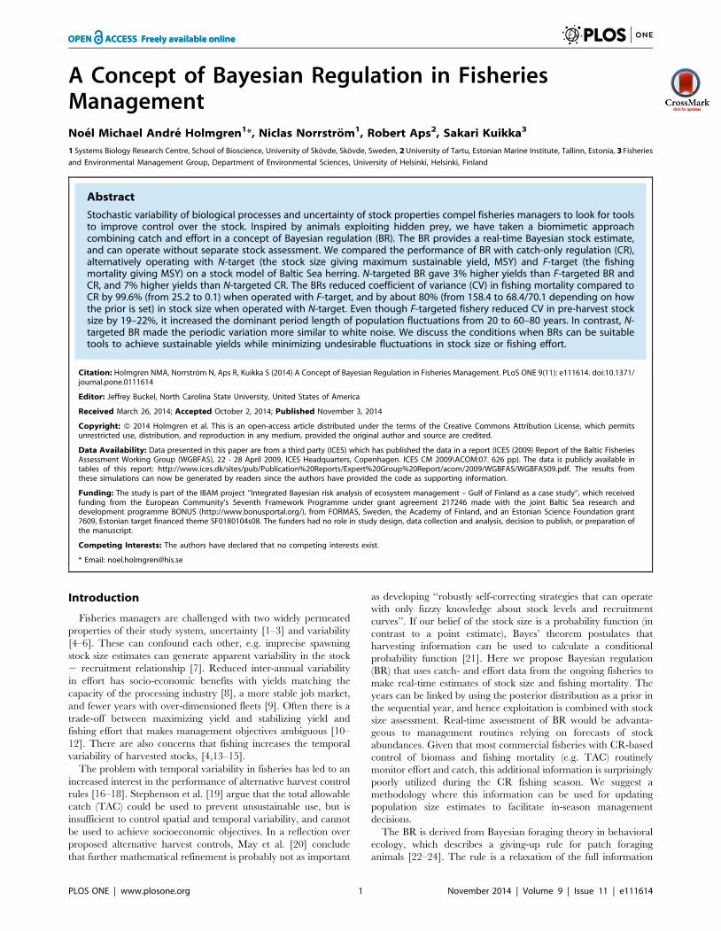
Figure 3. Average yields and confidence intervals as functionsof increasing length of simulation in years. Filled symbols denotesupervised and open symbols unsupervised harvest control. Squaresdenote CR and circles BR. Solid lines denote N-target managementwhereas hatched lines denote F-targeted management.doi:10.1371/journal.pone.0111614.g003

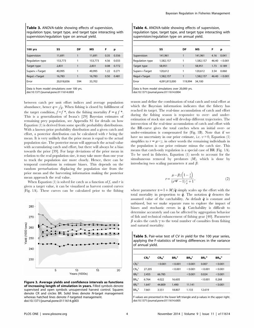
Table 3. ANOVA-table showing effects of supervision,regulation type, target type, and target type interacting withsupervision/regulation type on annual yield.

100 yrs SS DF MS F p

Supervision 11,691 1 11,691 0.35 0.556

Regulation type 153,773 1 153,773 4.56 0.033

Target type 2,831 1 2,831 0.08 0.772

Superv.6Target 40,995 1 40,995 1.22 0.271

Regul.6Target 16,783 1 16,783 0.50 0.481

Error 20,018,836 594 33,702

Data is from model simulations over 100 yrs.doi:10.1371/journal.pone.0111614.t003

Table 4. ANOVA-table showing effects of supervision,regulation type, target type, and target type interacting withsupervision/regulation type on annual yield.

SS DF MS F p

Supervision 141,961 1 141,961 4.16 0.041

Regulation type 1,582,157 1 1,582,157 46.40 ,0.001

Target type 58,951 1 58,951 1.73 0.189

Superv6Target 120,612 1 120,612 3.54 0.060

Regul6Target 1,582,157 1 1,582,157 46.40 ,0.001

Error 4,091,815,000 119,994 34,100

Data is from model simulations over 20,000 yrs.doi:10.1371/journal.pone.0111614.t004

Table 5. Pair-wise test of CV in yield for the 100 year series,applying the F-statistics of testing differences in the varianceof annual yield.

CRFs CRN

s BRFs BRN

s BRFu BRN

u

CRFs ,0.001 ,0.001 ,0.001 0.007 ,0.001

CRNs 27.205 ,0.001 ,0.001 ,0.001 ,0.001

BRFs 2.455 66.785 ,0.001 0.024 ,0.001

BRNs 6.764 4.022 16.605 ,0.001 0.268

BRFu 1.647 44.809 1.490 11.141 ,0.001

BRNu 7.661 3.551 18.807 1.133 12.619

F-values are presented in the lower left triangle and p-values in the upper right.doi:10.1371/journal.pone.0111614.t005



b~1{e{ Mzqqð Þf

1{e{qqfð3Þ

Note that b depends on effort such that Equation (2) can work as a

real-time estimator of the population size. The Bayesian estimator

is used with the different targets (Table 1). When the target is

formulated as a post-harvest population size (N’MSY), harvesting

should stop when the Bayesian estimate of remaining stock size (r)

equals target N’MSY:

re{ 1{fð ÞM~N ’MSY ð4Þ

The target N’MSY denotes the stock size at the end of the year,

we therefore need to take into account the removal of individuals

due to natural mortality for the remaining part of the year after

fishing has ended, e{ 1{fð ÞM . When our target is defined as fishing

mortality, FMSY, harvesting is aborted when.

cbczr

~1{e{FMSY ð5Þ

Note that the prior m cannot be used in the denominator,

because the estimated size of the pre-harvest population changes

as we receive information from catch and effort. When the

conditions in Equation (4), or (5) are fulfilled, we extract the fishing

effort (f*) from Equation (2). Equations (2), (4) and (5) together

define the control rules both for CR and BR.

Assessment and priorsEstimates of the pre-harvest stock size, the prior m, are produced

in two ways: by supervised assessment and unsupervised assess-

ment (Table 1). Supervised assessment represents the current

annually revised assessment practiced by ICES and other stock

assessors. In this case, m is calculated by adding an assessment

error to the actual pre-harvest stock size, N. The error is a random

value drawn from a normal distribution with mean = 0, and

variancev which is equal to the variance of the pre-harvest stock

size in the FMSY-analysis (see below). The coefficient of variance in

the FMSY-analysis is 21%. This represents an ideal assessment

where the error solely stems from the yearly variation of the

population when fished at FMSY. The unsupervised assessment

uses m equal to the average, and v the variance of the pre-harvest

stock size from the FMSY -analysis (i.e. when fishing at FMSY; see

below). The rationale of using a constant m is that the Bayesian

information of stock size when a fishery has been closed in the

foregoing year indicates N’MSY at the end of the year when using

N-target (Equation 4). Similarly for an F-targeted fishery, fishing is

closed every year when at estimated FMSY, which is associated

with the mean N’ = N’MSY. The variance is used for the BR,

whereas v = 0 for the CR.

The stochastic operating modelWe have used a stock model of the herring population in the

main basin of the Baltic Sea (ICES catch area subdivisions 25–27,

28.2, 29 and 32) for harvest control evaluation. The model is a

stochastic operating model (SOM) parameterized from statistical

analyses of ICES catch data and outputs from ICES XSA runs

(Appendix S2).

MSY analysisWe performed an MSY-analysis on the SOM by stepping the

fishing mortality in steps of 0.01, and for each F-value simulating

40,000 years and rejecting the first 500 to minimize the effects of

initiation values. In contrast to simulated management, this

algorithm executes perfectly-controlled constant fishing mortality.

The relationship between yield and fishing mortality was used to

identify the FMSY and its associated average post-harvest stock size.

These were used as targets for F-targeted and N-targeted

management, respectively. The average pre-harvest stock size,

given fishing mortality FMSY, was used as the prior (m) in the

unsupervised simulations, and the variance in the pre-harvest stock

size was used as a measure of the uncertainty (v) of m in the BR.

The lower 2.5% percentile of the associated SSB was used as the

Btrigger. Targets, priors and assessment modes were used in

Table 7. ANOVA-table showing effects of supervision, regulation type, target type, and target type interacting with supervision/regulation type on annual fishing mortality.

SS DF MS F p

Supervision 0.00047 1 0.00047 0.02 0.886

Regulation type 0.03166 1 0.03166 1.40 0.236

Target type 0.02945 1 0.02945 1.31 0.254

Superv6Target 0.00046 1 0.00046 0.02 0.886

Regul6Target 0.03265 1 0.03265 1.45 0.229

Error 13.39279 594 0.02255


Table 6. Mean, standard deviation and CV (%) of annualfishing mortality (F) of 100 years of simulated fishing.

mean SD CV

CRFs 0.17 0.043 25.2

CRNs 0.20 0.325 158.4

BRFs 0.17 0.000 0.1

BRNs 0.17 0.118 70.1

BRFu 0.17 0.000 0.1

BRNu 0.17 0.119 68.4

FMSY from the FMSY -analysis is 0.17.doi:10.1371/journal.pone.0111614.t006



defining the eight different HCRs, all aiming at achieving MSY

(Table 1).

Evaluation of harvest control rulesThe eight HCRs were applied to Monte Carlo simulations of

the SOM. A simulation started with a number of years of

controlled fishing with FMSY to get away from the initial

population size and age-structure. After the initial period, data

was collected for a number of years of applied HCR. We ran

shorter time series with an initiation period of 1,000 years and 100

years of applied HCR. The time period of 100 years reflects a

reasonably long time-horizon for management. We also ran longer

series with an initiation period of 100 years and 20,000 years of

applied HCR, in order to establish more accurate estimates of

mean yields. We collected annual data on yield, fishing mortality,

pre-harvest and post-harvest population size, and SSB. Cod SSB

and year-specific growth were kept at a mean level (Cy = 100,000

tons, ky = 0) during the simulations with the addition of random

noise, the size of which was extracted from historical data after

removing long-term changes [31]. Technically, fishing on the

SOM is performed by applying the effort, f*, from the solution of

the quitting rules in Equation (4) and (5). f* is calculated by halved-

distance iterations until the estimate (the left side of Equation 4

and 5) differed from the target with less than 0.1%. The

population is harvested by stepping the SOM one year with the

catch being determined by Baranov’s catch equation:

c~qf �

Mzqf �m 1{e{ Mzq f �ð Þ� �

, ð6Þ

in which we use the actual q of the SOM.

Sensitivity to error in catchabilityWe keep the estimated catchability qq in Equation (2) and (3)

constant and unbiased in our base runs, but fishery dependent

catchability may in reality be biased and vary over time. Such

uncorrelated errors and biases in catchability will contribute to

error or bias in the assessment. Our base model already has

assessment error (CV = 21%, as described in Assessment andpriors) for supervised HCRs, but unsupervised BRs do not

(Table 1). Unsupervised BRs do not use separate assessments,

but on the other hand they will be affected by error or bias in qq.

We chose to compare supervised F-targeted CR and unsupervised

F-targeted BR because the former is only affected by the error in

Table 8. Pair-wise test of CV-values applying the F-statistics of testing differences in the variance of annual fishing mortality.

CRFs CRN

s BRFs BRN

s BRFu BRN

u

CRFs ,0.001 ,0.001 ,0.001 ,0.001 ,0.001

CRNs 39.520 ,0.001 ,0.001 ,0.001 ,0.001

BRFs 67,742 2,677,131 ,0.001 0.066 ,0.001

BRNs 7.731 5.112 523,678 ,0.001 0.404

BRFu 49,987 1,975,470 1.355 386,425 ,0.001

BRNu 7.361 5.369 498,613 1.050 367,930


Figure 4. Fishing mortality (F) for 100 years for different HCRs. The dashed reference line is the FMSY = 0.17 obtained from the FMSY-analysisduring controlled F.doi:10.1371/journal.pone.0111614.g004



the assessed stock size, m, whereas the latter is affected only by the

error in qq. We also explored the sensitivity to correlated biases in

qqand m by changing their values 620%. Simulations ran for

41,000 generations and data from the last 40,000 were used for the

analyses.

Statistical analysesUnsupervised CR expectedly led to population crashes within a

few decades or less. We therefore excluded them in the statistical

analyses, which were performed using STATISTICA software

(Statsoft, Tulsa, Oklahoma). General linear models (GLM) were

used for three-way ANOVAs, testing the effects of supervision

mode, regulation type and target type on yield, fishing mortality,

spawning stock biomass, and post-harvest population size. Fourier

analyses were performed on 1,000 year data series, tapered by

15% and padded to the length power of 2. The period length in

years with the highest spectral density was identified after applying

Hamming weights with a data window of size 7. Test of significant

deviation from white noise was performed using Kolmogorov-

Smirnov deviation (d) statistics, Table Y, r = 0.5, n.100 in Rohlf

& Sokal [41].

Results

YieldMean yield in 100-year simulations is significantly higher with

BR than with CR although the differences are small (Fig. 2,

Table 2, 3). With an increasing length of the time series the

confidence intervals narrow (Fig. 3). Analysis of 20,000 years

reveals more clearly that BRs operated with N-target give the

highest average yields, even though the largest differences in

means are less than 10% (Table 2, 4). Supervised and unsuper-

vised BRs give higher yields (262 thousand tons) than the reference

MSY from the FMSY -analysis (254 thousand tons; Table 2, 3, 4,

5). Contrary to the small differences in mean yields, the CV in

yields is clearly affected by the choice of HCR. In general, using F-

targets gave less temporal variation than using N-targets (Fig. 2,

Table 2, 3, 4, 5). There is also an effect of regulation type with BR,

giving less variation than CR (Fig. 2, Table 3, 4). However,

supervised BR and unsupervised BR have the same CV regardless

of target (Table 5).

Figure 5. Post-harvest N-values for different HCRs in simulations over 100 years. The dashed reference line is the N-target = 41,491 millionobtained from the FMSY analysis during controlled F.doi:10.1371/journal.pone.0111614.g005

Table 9. Mean (Million), standard deviation and CV (%) ofannual post-harvest population size, N’, of 100 years ofsimulated fishing.

mean SD CV

CRFs 42,620 9,201 21.6

CRNs 34,282 9,470 27.6

BRFs 44,391 8,798 19.8

BRNs 41,508 1,616 3.9

BRFu 42,270 7,248 17.1

BRNu 41,569 1,840 4.4

N-target from the FMSY -analysis is 41,491 million.doi:10.1371/journal.pone.0111614.t009



Fishing mortalityThere is no significant difference in mean fishing mortality (F)

due to any effect over 100 years (Table 6, Table 7). All HCRs

reach the F-target of 0.17 as their mean, except supervised CR

with N-target, which has a mean F of 0.20. Although the mean Fs

are very similar across HCRs, the differences in CV are more

pronounced. Supervised CR with N-target exhibits the highest CV

of 158% (Table 6). F-targeted supervised CR has a CV of 25%

(Table 6, Fig. 4). Since catchability is constant here, F is

proportional to fishing effort. It is therefore not surprising that

F-targeted HCRs result in less variation than N-targeted HCRs.

F-targeted BRs, supervised and unsupervised, show very high

precision in reaching the target (Fig. 4), the CV being as low as

0.1% (Table 6). As expected, N-targeted BRs exhibit higher CVs

(68% unsupervised and 70% supervised; Table 6). In addition, it is

only the CV between supervised and unsupervised BRs that does

not differ significantly from each other (Table 8).

Post-harvest population size and SSBLooking at post-harvest population size (N’), the harvest controls

operating on N-targets are aiming for 41.5 billion individuals at

the end of the year. The two N-targeted BRs reach this target with

little variation between years (4% CV; Fig. 5, Table 9, 10, 11),

whereas N-targeted CR leads to over-fishing in the sense that N’ is

on average 17% below target. In contrast to the N-targeted

regulation types, there is a small difference in N’ between F-

targeted BR and CR. This explains the significant interaction

between regulation type and target type in the ANOVA

(Table 10). Supervision has no significant effect on the mean N’

(Table 10), nor the CV (Table 11).

The mean SSBs differ significantly by regulation type, harvest

type and supervision (Table 12). BR SSBs are on average larger

than CR SSBs (Fig. 6, Table 13, 13). Supervised CR with N-

target has the lowest mean and is below Btrigger in 50% of the years

(Table 13, Fig. 6). Supervised BRs has on average larger SSBs

than unsupervised, and the BRs operating with N-targets surpass

the Btrigger less frequently than when operating with F-targets

(Table 13, Fig. 6). The lower CV for BRs operating with N-target

(Table 13, 14) seems to be the main reason for this result.

Bias and error in harvest ratesSo far we can summarize the difference between CR and BR as

being BR’s ability to reduce the variance in the target variable (For N’; Tables 3, 4). Yield is partially dependent on F, and SSB on

N’, and thus the variance of these variables is also reduced,

although to a lesser degree (Tables 2, 5). These results are based

on the assumption of a constant and un-biased estimate of

catchability (qq). When random error is added to the catchability (q)

of the same magnitude as the error in m, the CV in c and F for the

unsupervised F-targeted BR become similar to supervised F-

targeted CR (Fig. 7). The two F-targeted harvest rules also

perform very similar in response to the off-set bias in m and qq.

Hence, supervised CR and unsupervised BR behave similarly

when error and bias in m and q are of the same relative magnitude.

Temporal variation in population sizeWe found that all HCRs decrease the amplitude of temporal

variation in pre- and post-harvest population numbers, except for

post-harvest numbers under supervised N-targeted CR, at which

the variation is indifferent from the unexploited population

(Table 15). The BR is effective in reaching the N-target, and

hence reduces the CV markedly in the post-harvest population size

(Fig. 8, Table 15). The effect is still evident in the pre-harvest

population size, in which the inclusion of recruits from the

foregoing year increases the variation (Table 15).

The unexploited population exhibited a very pronounced

periodicity of about 20 years (Fig. 8, Table 16). There is only

uncorrelated variation in our operating model, which means that

any periodicity is due to the demographic parameters and

structure of the population. The BRs with N-target remove much

of this periodicity and puts it closer to white noise (Lower K-S d-

values, Table 16). HCRs with F-target increase the dominating

period length to about 70–80 years (Table 16). Supervised CR

with F-target, a simplified version of the HCR currently used,

Table 10. ANOVA-table showing effects of supervision,regulation type, target type, and target type interacting withsupervision/regulation type on annual post-harvestpopulation size.

SS DF MS F p

Supervision 1.06E+08 1 1.06E+08 2.1 0.153

Regulation type 2.02E+09 1 2.02E+09 39.1 ,0.001

Target type 2.44E+09 1 2.44E+09 47.2 ,0.001

Superv6Target 1.19E+08 1 1.19E+08 2.3 0.130

Regul6Target 7.44E+08 1 7.44E+08 14.4 ,0.001

Error 3.07E+10 594 5.17E+07


Table 11. Pair-wise test of CV-values applying the F-statisticsof testing differences in the variance of annual post-harvestpopulation size.

CRFs CRN

s BRFs BRN

s BRFu BRN

u

CRFs 0.007 0.198 ,0.001 0.011 ,0.001

CRNs 1.637 0.001 ,0.001 ,0.001 ,0.001

BRFs 1.187 1.943 ,0.001 0.076 ,0.001

BRNs 30.736 50.318 25.903 ,0.001 0.103

BRFu 1.585 2.595 1.336 19.387 ,0.001

BRNu 23.800 38.964 20.058 1.291 15.012


Table 12. ANOVA-table showing effects of supervision,regulation type, target type, and target type interacting withsupervision/regulation type on annual SSB.

SS DF MS F p

Supervision 1 054 971 1 1 054 971 19.8 ,0.001

Regulation type 6 757 878 1 6 757 878 126.9 ,0.001

Target type 2 008 542 1 2 008 542 37.7 ,0.001

Superv6Target 164 153 1 164 153 3.1 0.080

Regul6Target 2 271 205 1 2 271 205 42.6 ,0.001

Error 31 642 602 594 53 270




reduces the amplitude of variation in both pre- and post-harvested

population size (Table 15). At the same time, it increases the

dominating period length from 20 years in the unexploited

population to about 80 years in the exploited (pre-harvest

population size, Table 16).

Discussion

We have suggested a new approach to fisheries regulation,

which we name Bayesian regulation (BR), and made a basic

evaluation of its properties in relation to catch-only regulation.

The idea of BR is adopted from Bayesian foraging theory, in

which patch-foragers are assumed to rely on a giving-up rule based

on prior information and sampling information [29,30,42]. The

Bayesian foraging theory has been studied extensively, including

the derivation of the probability function used and that cumulative

catch and effort are sufficient information variables [29]. The BR

uses the uncertainty of the stock size estimate as a parameter,

which is rarely the case in current management [43–45], and

which has been requested for some time [46]. The general

applicability of the BR is emphasized by the fact that catch-only

regulation, (CR), is a special case of BR _ i.e. when there is no

uncertainty in the prior estimate of the stock size from an

assessment or survey. We have analyzed three aspects of harvest

controls: (i) the relevance of supervision (with or without stock size

assessment), (ii) operational target type (constant fishing mortality,

F, or constant stock size, N), (iii) type of regulation (catch

only = CR, or Bayesian evaluation of combined catch and

effort = BR), and their effect on mean and variance in yield and

stock size.

The effect of fishing on stock dynamicsThere is an ongoing discussion about whether fishing leads to

increased temporal variability in stock size compared to unex-

ploited populations [4,14]. Observations from California, USA,

corroborate the view that fishing magnifies fluctuations in fish

abundance, driven by increased intrinsic growth rates as a

response to higher mortality [4]. Models without age-structure

show an increased variability in population abundance as a

consequence of exploitation [14]. In a structured model, fishing

can either increase or decrease the stock size variability [15]. We

find that the CV of population size has been reduced in all

investigated HCRs, and especially with N-targeted BR. The

different effects of fishing between our and the previous studies

Figure 6. Spawning stock biomass (SSB) for different HCRs in simulations over 100 years. The dashed reference line is the Btrigger = 988thousand tons. It is the 2.5% lower percentile of SSB obtained from the FMSY-analysis during controlled F.doi:10.1371/journal.pone.0111614.g006

Table 13. Mean in thousand tons, standard deviation and CV (%) of annual SSB of 100 years of simulated fishing.

mean SD CV ,Btrigger (%)

CRFs 1 240 230.0 18.6 26.1

CRNs 906 308.6 34.1 49.9

BRFs 1 349 232.8 17.3 18.3

BRNs 1 317 192.4 14.6 5.6

BRFu 1 206 245.1 20.3 20.6

BRNu 1 255 142.3 11.3 5.9

The percentage of years the SSB surpassed the Btrigger (Btrigger = 998 thousand tons), is given in the rightmost column.doi:10.1371/journal.pone.0111614.t013



Table 14. Pair-wise test of CV in yield for the 100 year series, applying the F-statistics of testing differences in the variance ofannual SSB.

CRFs CRN

s BRFs BRN

s BRFu BRN

u

CRFs ,0.001 0.236 0.009 0.183 ,0.001

CRNs 3.368 ,0.001 ,0.001 ,0.001 ,0.001

BRFs 1.156 3.894 0.049 0.053 ,0.001

BRNs 1.614 5.434 1.396 0.001 0.006

BRFu 1.200 2.807 1.387 1.936 ,0.001

BRNu 2.678 9.018 2.316 1.660 3.213


Figure 7. A comparison of yield, fishing mortality (F), post-harvest stock size (N’) and spawning stock biomass (SSB) when randomerrors of the same CV are applied to both the stock size assessment (m) and the estimated catchability parameter (qq). Relative positiveand negative biases applied to qq and m are denoted on the x-axis. Circles denote results from F-targeted unsupervised BR and squares F-targetedsupervised CR. Black symbols denote the value (left axis) and grey symbols the CV of the effect-variable (right axis).doi:10.1371/journal.pone.0111614.g007



may depend on our implementation of errors in assessment,

whereas earlier studies implemented perfect fishing mortality.

The comparison of Bayesian- and catch-regulationWe expected N-targeted BR to give the highest mean yields,

because of its ability to maintain the population in the most

productive state. It turned out to return the highest mean yield,

but the differences between HCRs are small. The CV of fishing

mortality and the population size is, however, much more affected

using BR compared to CR. The advantage of F-targeted BR is

seen in a reduced variation in fishing mortality and yield.

Similarly, the N-targeted BR is associated with less variation in

post-harvest population size and SSB. Under some conditions CR

can be a blunt harvest control instrument; populations inevitably

go extinct if not supervised, and it exhibits the largest CV in yield,

F and SSB of all harvest controls when operated with N-target.

For the better, F-target supervised CR is a commonly applied

harvest control, e.g. within the European Union, and exhibits a

smaller CV than N-targeted CR in all fisheries and stock variables

investigated. Choosing BR, a manager has to consider the trade-

off between the pros and cons of an F- versus an N-targeted

fishery, since targeting one variable pushes the variability to the

other [47]. From a fisheries perspective, F-targeted BR can appear

as the most preferable HCR: low variability in effort (costs) and

yield (income) enables a more stable economy, and an even

process load is more manageable for the food industry [47]. At the

same time, single-stock F-targeted BR can potentially yield a

conflict of interest between fishers, and may be less desirable when

taking into account the ecological interaction between different

species of fish. N-targeted BR, on the other hand, gives low

variation in population size, which means lower risks of extinction

and smaller indirect effects of variability on prey and predator

species, which may also be subject to commercial fishing. The

stable post-harvest population size of N-targeted BR, in combi-

nation with the inherent variation in the productivity of the

population causes a highly variable yield.

Table 15. Coefficient of variation (CV) of pre- and post-harvest population numbers compared with the unexploited population.

Pre-harvest N Post-harvest N

CV F-value p CV F-value p

CRFs 21.6 1.52 ,0.001 22.0 1.42 ,0.001

CRNs 24.5 1.18 ,0.001 26.1 1.00 n.s.

BRFs 21.2 1.57 ,0.001 21.2 1.53 ,0.001

BRNs 14.8 3.25 ,0.001 4.6 33.01 ,0.001

BRFu 20.8 1.64 ,0.001 20.7 1.60 ,0.001

BRNu 15.1 3.12 ,0.001 4.7 30.58 ,0.001

Unexpl. Pop. 26.6 26.1

CV is from simulations of 10,000 years. F-value is the ratio of squared CVs (i.e. comparison of standardized variances).doi:10.1371/journal.pone.0111614.t015

Figure 8. Spectral densities of Fourier analysis of 1,000 years of pre-harvest population size under various HCRs. Period lengths from0 to 100 years are shown (depicted on the abscissa).doi:10.1371/journal.pone.0111614.g008



Our results show that F-targeted BRs come close to resolving

the trade-off between a high long-term yield and the stable fishing

effort and yield acknowledged by some authors [20,35]. Although

giving a slightly lower average yield than BRs with N-target, the

yield is higher than with CR and the fluctuations in the yield are

reduced considerably.

The ability of the BR to control the target variable depends on

the reliability of the estimated fishery-dependent catchability. We

have shown, as a rule of thumb, that if the CV of the error in

catchability is as large as the error CV in the stock size assessment,

the unsupervised BR performs similar to the supervised CR. Lack

of knowledge makes it difficult to say in general which of the errors

is the largest, in fishery-dependent catchability or in assessments.

In the case of the Newfoundland cod, CPUE increased when stock

abundance declined due to hyper-aggregation of the fish [40].

Such deceitful behavior of CPUE warrants close attention, and

neither BRs nor CRs are immune to it. It is possible to estimate

catchability accurately when we know the fishing gear, the fishers’

behavior, and the fish dispersal pattern. One could say that a

transfer from CR to BR would require a shift of focus by managers

from surveys and assessments to gear efficiency, behavior of fish

and fishing fleets.

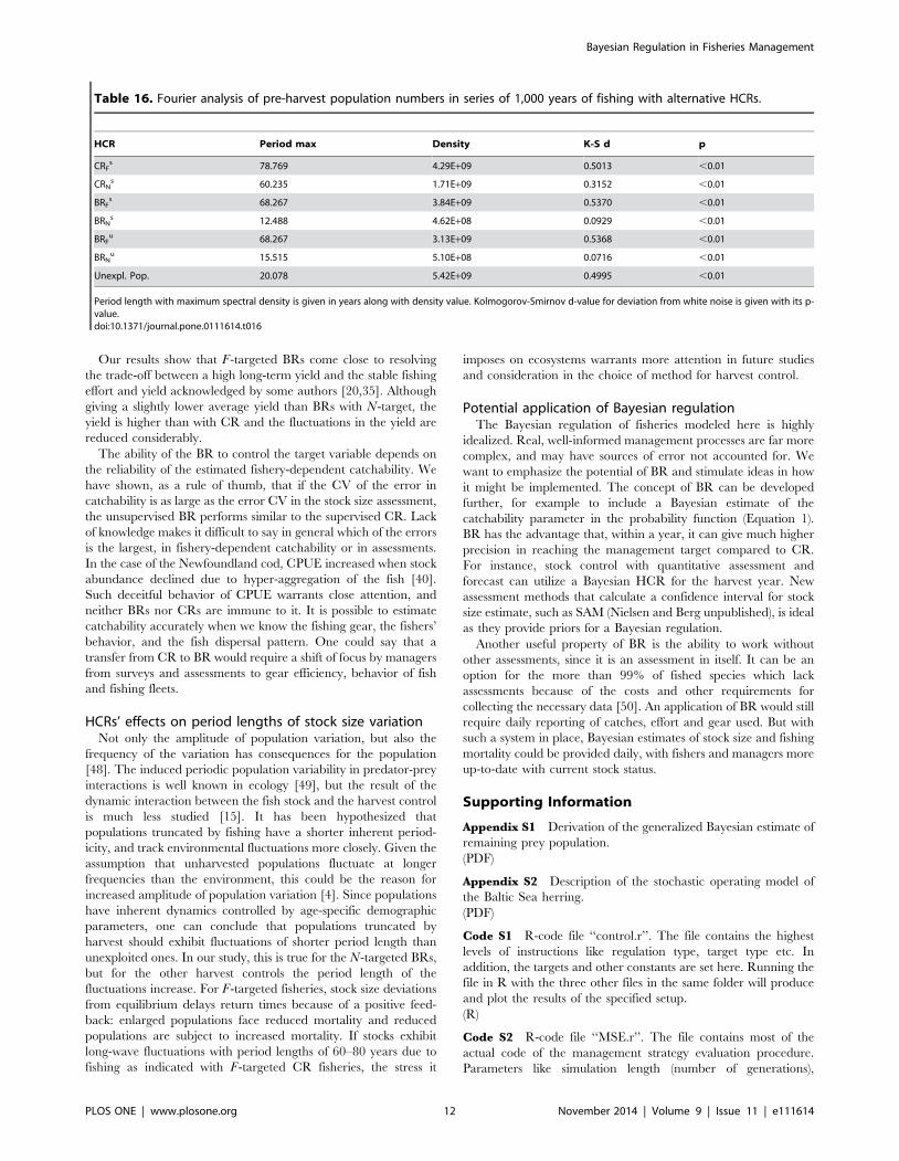
HCRs’ effects on period lengths of stock size variationNot only the amplitude of population variation, but also the

frequency of the variation has consequences for the population

[48]. The induced periodic population variability in predator-prey

interactions is well known in ecology [49], but the result of the

dynamic interaction between the fish stock and the harvest control

is much less studied [15]. It has been hypothesized that

populations truncated by fishing have a shorter inherent period-

icity, and track environmental fluctuations more closely. Given the

assumption that unharvested populations fluctuate at longer

frequencies than the environment, this could be the reason for

increased amplitude of population variation [4]. Since populations

have inherent dynamics controlled by age-specific demographic

parameters, one can conclude that populations truncated by

harvest should exhibit fluctuations of shorter period length than

unexploited ones. In our study, this is true for the N-targeted BRs,

but for the other harvest controls the period length of the

fluctuations increase. For F-targeted fisheries, stock size deviations

from equilibrium delays return times because of a positive feed-

back: enlarged populations face reduced mortality and reduced

populations are subject to increased mortality. If stocks exhibit

long-wave fluctuations with period lengths of 60–80 years due to

fishing as indicated with F-targeted CR fisheries, the stress it

imposes on ecosystems warrants more attention in future studies

and consideration in the choice of method for harvest control.

Potential application of Bayesian regulationThe Bayesian regulation of fisheries modeled here is highly

idealized. Real, well-informed management processes are far more

complex, and may have sources of error not accounted for. We

want to emphasize the potential of BR and stimulate ideas in how

it might be implemented. The concept of BR can be developed

further, for example to include a Bayesian estimate of the

catchability parameter in the probability function (Equation 1).

BR has the advantage that, within a year, it can give much higher

precision in reaching the management target compared to CR.

For instance, stock control with quantitative assessment and

forecast can utilize a Bayesian HCR for the harvest year. New

assessment methods that calculate a confidence interval for stock

size estimate, such as SAM (Nielsen and Berg unpublished), is ideal

as they provide priors for a Bayesian regulation.

Another useful property of BR is the ability to work without

other assessments, since it is an assessment in itself. It can be an

option for the more than 99% of fished species which lack

assessments because of the costs and other requirements for

collecting the necessary data [50]. An application of BR would still

require daily reporting of catches, effort and gear used. But with

such a system in place, Bayesian estimates of stock size and fishing

mortality could be provided daily, with fishers and managers more

up-to-date with current stock status.

Supporting Information

Appendix S1 Derivation of the generalized Bayesian estimate of

remaining prey population.

(PDF)

Appendix S2 Description of the stochastic operating model of

the Baltic Sea herring.

(PDF)

Code S1 R-code file ‘‘control.r’’. The file contains the highest

levels of instructions like regulation type, target type etc. In

addition, the targets and other constants are set here. Running the

file in R with the three other files in the same folder will produce

and plot the results of the specified setup.

(R)

Code S2 R-code file ‘‘MSE.r’’. The file contains most of the

actual code of the management strategy evaluation procedure.

Parameters like simulation length (number of generations),

Table 16. Fourier analysis of pre-harvest population numbers in series of 1,000 years of fishing with alternative HCRs.

HCR Period max Density K-S d p

CRFs 78.769 4.29E+09 0.5013 ,0.01

CRNs 60.235 1.71E+09 0.3152 ,0.01

BRFs 68.267 3.84E+09 0.5370 ,0.01

BRNs 12.488 4.62E+08 0.0929 ,0.01

BRFu 68.267 3.13E+09 0.5368 ,0.01

BRNu 15.515 5.10E+08 0.0716 ,0.01

Unexpl. Pop. 20.078 5.42E+09 0.4995 ,0.01

Period length with maximum spectral density is given in years along with density value. Kolmogorov-Smirnov d-value for deviation from white noise is given with its p-value.doi:10.1371/journal.pone.0111614.t016



predator spawning stock biomass, and other parameters are set in

this file.

(R)

Code S3 R-code file ‘‘BR.r’’. The file contains the algorithm to

produce the fishing mortality that the BR suggests. The error and

bias of A are set here, as is the tolerance of the algorithm. This

code is used both for CR and BR where catch only regulation

results are produced by having the variance set to zero.

(R)

Code S4 R-code file ‘‘OPMOD.r’’. The file contains the

stochastic operating model. The parameters that are more directly

linked to the population are set here, as are also the initial values of

the population numbers-at-age and weights-at-age. The functions

that describe mortality, reproduction, growth, and the weight of

one year olds are defined here.

(R)

Acknowledgments

Dr. Michael Errigo and an anonymous reviewer gave valuable comments

on the manuscript. Oskar MacGregor provided improvements on the

language.

Author Contributions

Conceived and designed the experiments: NMAH NN RA SK. Performed

the experiments: NMAH NN. Analyzed the data: NMAH NN RA SK.

Contributed reagents/materials/analysis tools: NMAH NN RA SK. Wrote

the paper: NMAH NN RA SK.

References

1. Virtala M, Kuikka S, Arjas E (1998) Stochastic virtual population analysis.ICES J Mar Sci 55: 892–904.

2. Mantyniemi S, Kuikka S, Rahikainen M, Kell LT, Kaitala V (2009) The value

of information in fisheries management: North Sea herring as an example.ICES J Mar Sci 66: 2278–2283.

3. Polasky S, Carpenter SR, Folke C, Keeler B (2011) Decision-making under greatuncertainty: environmental management in an era of global change. Trends

Ecol Evol 26: 398–404.4. Anderson CNK, Hsieh C, Sandin SA, Hewitt R, Hollowed A, et al. (2008) Why

fishing magnifies fluctuations in fish abundance. Nature 452: 835–839.

5. Jonzen N, Ripa J, Lundberg P (2002) A Theory of Stochastic Harvesting inStochastic Environments. Am Nat 159: 427–437.

6. Getz WM (1985) Optimal and Feedback Strategies for Managing MulticohortPopulations. J Optimiz Theory App 46: 505–514.

7. Walters CJ, Ludwig D (1981) Effects of Measurement Errors on the Assessment

of Stock-Recruitment Relationships. Can J Fish Aquat Sci 38: 704–710.8. Hjerne O, Hansson S (2001) Constant catch or constant harvest rate? Baltic Sea

cod (Gadus morhua L.) fishery as a modelling example. Fish Res 53: 57–70.9. Aps R, Fetissov M, Holmgren N, Norrstrom N, Kuikka S (2011) Central Baltic

Sea herring: effect of environmental trends and fishery management. In:Villacampa Y, Brebbia CA, editors. Ecosystems and Sustainable Development

VIII. Boston: WIT Press Southampton. pp. 69–80.

10. Hightower JE, Grossman GD (1985) Comparison of constant effort harvestpolicies for fish stocks with variable recruitment. Can J Fish Aquat Sci 42: 982–

988.11. Koonce JF, Shuter BJ (1987) Influence of Various Sources of Error and

Community Interactions on Quota Management of Fish Stocks. Can J Fish

Aquat Sci 44: s61–s67.12. Murawski SA, Idoine JS (1989) Yield Sustainability under Constant-Catch

Policy and Stochastic Recruitment. T Am Fish Soc 118: 349–367.13. Hsieh C, Reiss CS, Hunter JR, Beddington JR, May RM, et al. (2006) Fishing

elevates variability in the abundance of exploited species. Nature 443: 859–862.14. Shelton AO, Mangel M (2011) Fluctuations of fish populations and the

magnifying effects of fishing. PNAS 108: 7075–7080.

15. Wikstrom A, Ripa J, Jonzen N (2012) The role of harvesting in age-structuredpopulations: disentangling dynamic and age-truncation effects. Theor Popul Biol

82: 348–354.16. Kell LT, Pilling GM, Kirkwood GP, Pastoors M, Mesnil B, et al. (2005) An

evaluation of the implicit management procedure used for some ICES roundfish

stocks. ICES J Mar Sci 62: 750–759.17. Kraak SBM, Kelly CJ, Codling EA, Rogan E (2010) On scientists’ discomfort in

fisheries advisory science: the example of simulation-based fisheries manage-ment-strategy evaluations. Fish and Fisheries 11: 119–132.

18. Rochet M-J, Rice JC (2009) Simulation-based management strategy evaluation:

ignorance disguised as mathematics? ICES J Mar Sci 66: 754–762.19. Stephenson R, Peltonen H, Kuikka S, Ponni J, Rahikainen M, et al. (2001)

Linking Biological and Industrial Aspects of the Finnish Commercial HerringFishery in the Northern Baltic Sea. In: Funk F, Blackburn J, Hay D, Paul AJ,

Stephenson R et al., editors. Herring: Expectations for a New Millennium.Fairbanks: University of Alaska Sea Grant. pp.741–760.

20. May RM, Beddington JR, Horwood JW, Shepherd JG (1978) Exploiting natural

populations in an uncertain world. Mathematical Biosciences 42: 219–252.21. Hilborn R, Mangel M (1997) The ecological detective. Princeton: Princeton

University Press.22. Dall SRX, Giraldeau L-A, Olsson O, McNamara JM, Stephens DW (2005)

Information and its use by animals in evolutionary ecology. Trends Ecol Evol 20:

187–193.23. McNamara JM, Green RF, Olsson O (2006) Bayes’ theorem and its applications

in animal behaviour. Oikos 112: 243–251.24. Valone TJ (1991) Bayesian and prescient assessment: foraging with pre-harvest

information. Anim Behav 41: 569–577.

25. Charnov EL (1976) Optimal foraging, the marginal value theorem. Theor PopulBiol 9: 129–136.

26. Olsson O, Holmgren NMA (1999) Gaining ecological information about

Bayesian foragers through their behaviour. I. Models with predictions. Oikos 87:251–263.

27. Olsson O, Wiktander U, Holmgren NMA, Nilsson SG (1999) Gaining ecological

information about Bayesian foragers through their behaviour. II. A field test with

woodpeckers. Oikos 87: 264–276.

28. Green RF (1980) Bayesian birds: a simple example of Oaten’s stochastic modelof optimal foraging. Theor Popul Biol 18: 244–256.

29. Iwasa Y, Higashi M, Yamamura N (1981) Prey distribution as a factor

determining the choice of optimal foraging strategy. Am Nat 117: 710–723.

30. Olsson O, Holmgren NMA (1998) The survival-rate-maximizing policy of

Bayesian foragers: wait for good news! Behav Ecol 9: 345–353.

31. Holmgren NMA, Norrstrom N, Aps R, Kuikka S (2012) MSY-orientatedmanagement of Baltic Sea herring (Clupea harengus) during different ecosystem

regimes. ICES J Mar Sci 69: 257–266.

32. ICES (2011) Report of the Workshop on Implementing the ICES Fmsy

Framework (WKFRAME-2), 10–14 February 2011, ICES, Denmark. ICES CM2011/ACOM: 33. 110 pp.

33. European Commission (2002) On the conservation and sustainable exploitation

of fisheries resources under the Common Fisheries Policy. Council regulation(EC) No 2371/2002.

34. Marchal P, Horwood J (1998) Increasing fisheries management options with aflexible cost function. ICES J Mar Sci 55: 213–227.

35. Pelletier D, Laurec A (1992) Management under uncertainty: defining strategies

for reducing overexploitation. ICES J Mar Sci 49: 389–401.

36. ICES (2009) Report of the ICES Advisory Committee, 2009. ICES Advice,

2009. Book 8, 132 pp.

37. ICES (2012) Report of the Workshop 3 on Implementing the ICES FmsyFramework, 9–13 January 2012, ICES, Headquarters. ICES CM 2012/ACOM

39: 1–33.

38. ICES (2012) Report of the ICES Advisory Committee 2012. ICES Advice, 2012.Book 8, 158 pp.

39. Valone TJ, Brown JS (1989) Measuring Patch Assessment Abilities of DesertGranivores. Ecology 70: 1800–1810.

40. Rose GA, Kulka DW (1999) Hyperaggregation of fish and fisheries: how catch-

per-unit-effort increased as the northern cod (Gadus morhua) declined.Can J Fish Aquat Sci 56: 118–127.

41. Rohlf FJ, Sokal RR (1995) Statistical tables. New York: W.H. Freeman & Co.

42. Green RF (1984) Stopping rules for optimal foragers. Am Nat 123: 30–43.

43. Patterson KR (1999) Evaluating uncertainty in harvest control law catches usingBayesian Markov chain Monte Carlo virtual population analysis with adaptive

rejection sampling and including structural uncertainty. Can J Fish Aquat Sci56: 208–221.

44. Prager MH, Porch CE, Shertzer KW, Caddy JF (2003) Targets and limits formanagement of fisheries: a simple probability-based approach. N Am J Fish

Manage 23: 349–361.

45. Shertzer KW, Prager MH, Williams EH (2008) A probability-based approach tosetting annual catch levels. Fish Bull 106: 225–232.

46. Patterson K, Cook R, Darby C, Gavaris S, Kell L, et al. (2001) Estimating

uncertainty in fish stock assessment and forecasting. Fish and Fisheries 2: 125–

157.

47. Getz WM, Francis RC, Swartzman GL (1987) On Managing Variable MarineFisheries. Can J Fish Aquat Sci 44: 1370–1375.

48. Ripa J, Lundberg P (1996) Noise colour and the risk of population extinctions.

Proc R Soc London B 263: 1751–1753.

49. Yodzis P (1991) Introduction to theoretical ecology. New York: Harper & Row.

50. Costello C, Ovando D, Hilborn R, Gaines SD, Deschenes O, et al. (2012) Status

and Solutions for the World’s Unassessed Fisheries. Science 338: 517–520.



a concept of bayesian regulation in fisheries management

Documents