A Concept of Environmental Forecasting and Variational Organization

of Modeling Technology

Vladimir Penenko

Institute of Computational Mathematics and Mathematical Geophysics SD RAS

Challenges of environment forecasting:

•Predictability of climate-environment system?

• Stability of climatic system?

• sensitivity to perturbations of forcing

Features of environment forecasting: uncertainty • in the long-term behavior of the climatic system;• in the character of influence of man-made factors in the conditions of changing climate

Uncertainty

• Discrepancy between models and real phenomena

• insufficient accuracy of numerical schemes and algorithms

• lack and errors of input data

A CONCEPT OF ENVIRONMENTAL FORECASTING

• Basic idea:

we use inverse modeling technique

to assess risk and vulnerability of territory

(object) with respect to harmful impact

in addition to traditional forecasting the state functions variability by forward methods

The methodology is based on:•control theory,•sensitivity theory,•risk and vulnerability theory,

•variational principles in weak-constrained formulation,•combined use of models and observed data,• forward and inverse modeling procedures,• methodology for description of links between regional and global processes ( including climatic changes) by means of orthogonal decomposition of functional spaces for analysis of data bases and phase spaces of dynamical systems

Theoretical background

Basic elements for concept implementation:

models of processes data and models of measurements global and local adjoint problems constraints on parameters and state functions functionals: objective, quality, control, restrictions etc. sensitivity relations for target functionals and

constraints feedback equations for inverse problems

( ) ( ) 0L Gt

Y B Y f r

0 0 ,a a Y Y ;

( )tD state function ,

( )tDY parameter vector. G “space” operator of the model

Variational form

( , , ) ( ( ), ) 0tD

I L dDdt Y Y

*( )tD adjoint functions , ,r ξ ς are the terms describing

uncertainties and errors of thecorresponding objects.

Mathematical model of processes

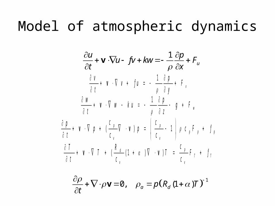
Model of atmospheric dynamics

1u

u pu fv kw F

t x

v

1v

v pv f u F

t y

v

1w

w pw k u g F

t z

v

( ) 1p pp p p

v v

c cpp p c F f

t c c

v v

( ( 1 ) ) pdT T

v v

cT RT T F f

t c c

v v

10, (1 )a dp R T

t

v

Transport and transformationof humidity

v

vv l f q

qq S S F

t

v

1l

ll l lT l q

qq q v S F

t z

v

1f

ff f fT f q

qq q v S F

t z

v

c

cc c q

qq S F

t

v

ii i i i i ii

L div ( grad ) ((S ) f (x, t) r ) 0,t

u

Transport and transformation modelof gas pollutants and aerosols

Operators of transformation

i r

j

R Us (q )

g i i jiq 1 j 1

S ( ) P( ) ( ) k(q) s (q ) s (q )

0

0

1 1 1 1 11 1

2

1 1 1 21

1,

2

,

, 1,

M

M M

a i ik k km kk m

M

i ik k i i i ik

i i i

S K d

K d e

R Q i M

Variational form of model’s set:hydrodynamics+ chemistry+ hydrological cycle

t

n

i i iii 1 D

I , ((S ) f (x, t) r ) dDdt

Y

t

* * * *p T

D

pp div pdiv pp TT div dDdt u u u

* 0t

npu d dt

t

T

a a a

D

W dDdt

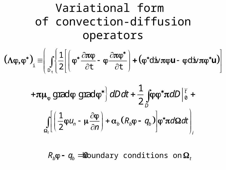
Variational form of convection-diffusion operators

t

iD

1div div

2 t t

u u

0

1grad grad

2t

D

dDdt dD

1

2t

n b b b

i

u R q d dtn

0b bR q boundary conditions on t

Model of observations

A set of measured data m , m on m

tD

[ ( )]m mH ,

[ ( )]mH models of observations.

the term describing uncertainty and errors adjoint function with respect to image of

observation mdDdt Radon’s or Dirac’s measure ) )m

t tD D

*5( , , ) [ ( )] 0

t

T

m m m m

D

I H W dDdt Y

Variational form

Goal functionals

( ) ( ) ( , ) , , 1,...,t

k k k k k

D

F t dDdt F k K x

kF are evaluated functions (differentiable in generilized sense, bounded,satisfying the Lipschitz's conditions), dDdtk are Radon’s or Dirac’s measures on tD , )(*

tk D .

Quality functionals for data assimilation

t

Tk m m m

D

H M H t dDdt x( ) ( ( )) ( ( )) ( , ) ,

mdDdt Radon’s or Dirac’s measures ) )mt tD D

Functionals for generalized description of information links in the system

Variational principle

* *

* *

( , , , , , , ) ( )

( , , ) ( , , )hkt

h hk k k

m DI I

Y r ξ ζ

Y

1 2 3 4 ( )0.5 ( ) ( ) ( ) ( )m h h h h

t t t

hT T T T

D D D R DW W W W r r ξ ξ ζ ζ

Augmented functional for computational technology

* *(, , ) / 0 ( , , , , , , , )h hk s s Y r ξ ζ

Algorithms for construction of numerical schemes

( , ) 0h

hktB G

Y f r

( ) ( , ) 0,h

T Tkt k k kB A

Y d

*5( ) ( ( ) ,

Thk k m

d H M

( ) 0k t t x

0 0 13 ( ,0), 0a kM t x

1 *2( , ) ( , ),kt M tr x x

14a kM Y Y

( , , )hk kI

YY

0( , ) ( , )hA G

Y Y

t i s t h e a p p r o x i m a t i o n o f t i m e d e r i v a t i v e sI n i t i a l g u e s s :

( 0 ) 0 ( 0 ) 0 ( 0 )0 , ,a a r Y Y

The universal algorithm of forward & inverse modeling

0( ) ( , Y) ( ,Y Y, )h hk k kI

0( ,Y Y, )Y

hk kI

The main sensitivity relations

Algorithm for calculation of sensitivity functions

Some elements of optimal forecasting and design

12 r x x*

k( ,t ) M ( ,t ),

13 0 0 xkM ( , ), t

1 14 4

hk kM M I ( ,Y , )

Y

Algorithms for uncertainty calculationbased on sensitivity analysis and

data assimilation:

in models of processes

in initial state

in model parameters and sources

1 5iM i,( , ) are weight matrices

15 1 x x* ( ,t ) M M ( ,t ),

in models of observations

Fundamental role of uncertainty functions

• integration of all technology components• bringing control into the system• regularization of inverse methods• targeting of adaptive monitoring • cost effective data assimilation

Optimal forecasting and design

Optimality is meant in the sense that estimations of the goal functionals do not depend on the variations :

• of the sought functions in the phase spaces of the dynamics of the physical system under study

• of the solutions of corresponding adjoint problems that generated by variational principles

• of the uncertainty functions of different kinds which explicitly included into the extended functionals

Construction of numerical approximations

• variational principle

• integral identity

• splitting and decomposition methods

• finite volumes method

• local adjoint problems

• analytical solutions

• integrating factors

1

* *1( ) ( )

jT

j js s mm m

s

H W H

Basic elements in frames of splitting and decomposition schemes:

p - number of stages

4DVar real time data assimilation algorithm

112. j j j j j

s s s s sf rt

1 *1 1,j j j

s s j jsr W t t t

1 111. , , 1, , 1j j

s jt t s p p

1

13. , , 1,

pj j

s js

t t j Jp

1

pjs

s

- operator of the model,

Scenario approach for environmental purposes

• Inclusion of climatic data via decomposition of phase spaces on set of orthogonal subspaces ranged with respect to scales of perturbations

• Construction of deterministic and deterministic-stochastic scenarios on the basis of orthogonal subspaces

• Models with leading phase spaces

Leading basis subspace for geopotential for 56 years

Leading basis subspace for horizontal velocities for 56 years

Leading orthogonal subspaces

36 years, 26.66% 46 years, 26.63%

56 years,26.34%

Risk/vulnerability assessmentSome scenarios for receptors

in Siberia

1

11

1

2

3

4

5

9 18 0.57 0.16 0.055 0.014 0.0053 0.0012 0.00051 0.0001

1

1

1

2

2

3457

9 18 0.57 0.16 0.055 0.014 0.0053 0.0012 0.00051 0.0001

Yakutsk

1

1

1

2

2

3

3

45

7

9 18 0.57 0.16 0.055 0.014 0.0053 0.0012 0.00051 0.0001

Khanti-Mansiisk

1

11

2

2

3

3

4

66

9 18 0.57 0.16 0.055 0.014 0.0053 0.0012 0.00051 0.0001

Krasnoyarsk

1

1

2

23

3

4

5

67

9 18 0.57 0.16 0.055 0.014 0.0053 0.0012 0.00051 0.0001

Mondy

1

1

1

3

23

3

3

4

5

6

7

9 18 0.57 0.16 0.055 0.014 0.0053 0.0012 0.00051 0.0001

Tomsk

1

1

1

2 23

4 6

9 18 0.57 0.16 0.055 0.014 0.0053 0.0012 0.00051 0.0001

Tory

1

1

2

2

3

4

76

9 18 0.57 0.16 0.055 0.014 0.0053 0.0012 0.00051 0.0001

Ulan-Ude1

1

1

2

2

3

3

4

45

9 18 0.57 0.16 0.055 0.014 0.0053 0.0012 0.00051 0.0001

Ussuriisk

Ekaterinburg

“climatic” April

Long-term forecasting for Lake Baikal regionRisk function

0.1

0.1

0.1

0.2

0.2

0.2

0.2

0.2

0.3

0.3

0.3

0.3

0.3

0.4

0.4

0.4

0.5

0.5

0.5

0.6

0.6

0.6

0.7

0.7

0.70.

8

0.8

0.9

0.9

95 100 105 110 115

50

55

60

Baikalsk

Irkutsk

Ulan-Ude

Nijhne-Angarsk

Cheremkhovo

Bratsk

Angarsk

Surface layer, climatic October

Conclusion

• Algorithms for optimal environmental

forecasting and design are proposed

• The fundamental role of uncertainty is highlighted

Thank you for your time!

number

eig

en

lavu

es

0 10 20 30

1

2

3

4

5

6

7

8

9

number

eig

en

lavu

es

10 20 30 40

1

2

3

4

5

6

7

8

9

10

11

12

number

eig

en

lavu

es

0 10 20 30 40 50

1

2

3

4

5

6

7

8

9

10

11

12

13

14

36 years

46 years

56 years

Separation of scales : climate/weather noise

Eigenvalues of Gram matrix as a measure of informativeness

of orthogonal subspaces

Risk assesment for Lake Baikal region

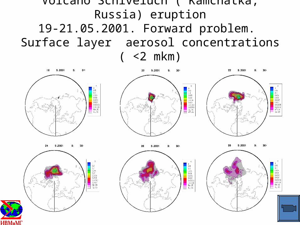
Volcano Schiveluch ( Kamchatka, Russia) eruption19-21.05.2001. Forward problem.

Surface layer aerosol concentrations ( <2 mkm)