a concise introduction to multiagent systems and …jmvidal.cse.sc.edu/library/vlassis07a.pdf ·...
TRANSCRIPT
MOBK077-FM MOBKXXX-Sample.cls August 3, 2007 7:54
A Concise Introductionto Multiagent Systemsand Distributed ArtificialIntelligence
i

MOBK077-FM MOBKXXX-Sample.cls August 3, 2007 7:54
ii

MOBK077-FM MOBKXXX-Sample.cls August 3, 2007 7:54
iii
Synthesis Lectures on ArtificialIntelligence and Machine Learning
EditorsRonald J. Brachman, Yahoo Research
Tom Dietterich, Oregon State University
Intelligent Autonomous RoboticsPeter Stone2007
A Concise Introduction to Multiagent Systems and Distributed Artificial IntelligenceNikos Vlassis2007
MOBK077-FM MOBKXXX-Sample.cls August 3, 2007 7:54
Copyright © 2007 by Morgan & Claypool
All rights reserved. No part of this publication may be reproduced, stored in a retrieval system, or transmitted inany form or by any means—electronic, mechanical, photocopy, recording, or any other except for brief quotationsin printed reviews, without the prior permission of the publisher.
A Concise Introduction to Multiagent Systems and Distributed Artificial Intelligence
Nikos Vlassis
www.morganclaypool.com
ISBN: 1598295268 paperbackISBN: 9781598295269 paperback
ISBN: 1598295276 ebookISBN: 9781598295276 ebook
DOI: 10.2200/S00091ED1V01Y200705AIM002
A Publication in the Morgan & Claypool Publishers series
SYNTHESIS LECTURES ON ARTIFICIAL INTELLIGENCE AND MACHINE LEARNINGSEQUENCE IN SERIES: #2
Lecture #2Series Editors: Ronald Brachman, Yahoo! Research and Thomas G. Dietterich, Oregon State University
First Edition
10 9 8 7 6 5 4 3 2 1
iv
MOBK077-FM MOBKXXX-Sample.cls August 3, 2007 7:54
A Concise Introductionto Multiagent Systemsand Distributed ArtificialIntelligenceNikos VlassisDepartment of Production Engineering and ManagementTechnical University of CreteGreece
SYNTHESIS LECTURES ON ARTIFICIAL INTELLIGENCE AND MACHINELEARNING SEQUENCE IN SERIES: #2
M&C M o r g a n & C l a y p o o l P u b l i s h e r s
v
MOBK077-FM MOBKXXX-Sample.cls August 3, 2007 7:54
vi
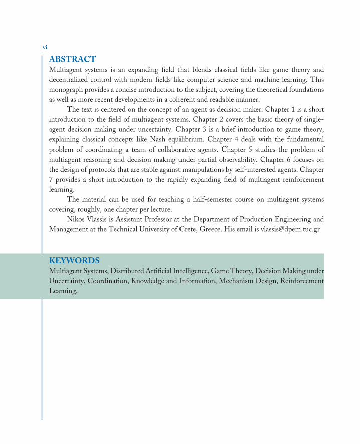
ABSTRACTMultiagent systems is an expanding field that blends classical fields like game theory anddecentralized control with modern fields like computer science and machine learning. Thismonograph provides a concise introduction to the subject, covering the theoretical foundationsas well as more recent developments in a coherent and readable manner.
The text is centered on the concept of an agent as decision maker. Chapter 1 is a shortintroduction to the field of multiagent systems. Chapter 2 covers the basic theory of single-agent decision making under uncertainty. Chapter 3 is a brief introduction to game theory,explaining classical concepts like Nash equilibrium. Chapter 4 deals with the fundamentalproblem of coordinating a team of collaborative agents. Chapter 5 studies the problem ofmultiagent reasoning and decision making under partial observability. Chapter 6 focuses onthe design of protocols that are stable against manipulations by self-interested agents. Chapter7 provides a short introduction to the rapidly expanding field of multiagent reinforcementlearning.
The material can be used for teaching a half-semester course on multiagent systemscovering, roughly, one chapter per lecture.
Nikos Vlassis is Assistant Professor at the Department of Production Engineering andManagement at the Technical University of Crete, Greece. His email is [email protected]
KEYWORDSMultiagent Systems, Distributed Artificial Intelligence, Game Theory, Decision Making underUncertainty, Coordination, Knowledge and Information, Mechanism Design, ReinforcementLearning.

MOBK077-FM MOBKXXX-Sample.cls August 3, 2007 7:54
vii
ContentsPreface . . . . . . . . . . . . . . . . . . . . . . . . . . . . . . . . . . . . . . . . . . . . . . . . . . . . . . . . . . . . . . . . . . . . . . . xi
1. Introduction . . . . . . . . . . . . . . . . . . . . . . . . . . . . . . . . . . . . . . . . . . . . . . . . . . . . . . . . . . . . . . . . . . 11.1 Multiagent Systems and Distributed AI . . . . . . . . . . . . . . . . . . . . . . . . . . . . . . . . . . . . 11.2 Characteristics of Multiagent Systems . . . . . . . . . . . . . . . . . . . . . . . . . . . . . . . . . . . . . . 1
1.2.1 Agent Design . . . . . . . . . . . . . . . . . . . . . . . . . . . . . . . . . . . . . . . . . . . . . . . . . . . . 11.2.2 Environment . . . . . . . . . . . . . . . . . . . . . . . . . . . . . . . . . . . . . . . . . . . . . . . . . . . . . 21.2.3 Perception . . . . . . . . . . . . . . . . . . . . . . . . . . . . . . . . . . . . . . . . . . . . . . . . . . . . . . . 21.2.4 Control . . . . . . . . . . . . . . . . . . . . . . . . . . . . . . . . . . . . . . . . . . . . . . . . . . . . . . . . . . 31.2.5 Knowledge . . . . . . . . . . . . . . . . . . . . . . . . . . . . . . . . . . . . . . . . . . . . . . . . . . . . . . . 31.2.6 Communication . . . . . . . . . . . . . . . . . . . . . . . . . . . . . . . . . . . . . . . . . . . . . . . . . . 3
1.3 Applications . . . . . . . . . . . . . . . . . . . . . . . . . . . . . . . . . . . . . . . . . . . . . . . . . . . . . . . . . . . . . 31.4 Challenging Issues . . . . . . . . . . . . . . . . . . . . . . . . . . . . . . . . . . . . . . . . . . . . . . . . . . . . . . . .51.5 Notes and Further Reading . . . . . . . . . . . . . . . . . . . . . . . . . . . . . . . . . . . . . . . . . . . . . . . . 5
2. Rational Agents . . . . . . . . . . . . . . . . . . . . . . . . . . . . . . . . . . . . . . . . . . . . . . . . . . . . . . . . . . . . . . . 72.1 What is an Agent? . . . . . . . . . . . . . . . . . . . . . . . . . . . . . . . . . . . . . . . . . . . . . . . . . . . . . . . .72.2 Agents as Rational Decision Makers . . . . . . . . . . . . . . . . . . . . . . . . . . . . . . . . . . . . . . . 72.3 Observable Worlds and the Markov Property . . . . . . . . . . . . . . . . . . . . . . . . . . . . . . . 8
2.3.1 Observability . . . . . . . . . . . . . . . . . . . . . . . . . . . . . . . . . . . . . . . . . . . . . . . . . . . . . 92.3.2 The Markov Property . . . . . . . . . . . . . . . . . . . . . . . . . . . . . . . . . . . . . . . . . . . . 10
2.4 Stochastic Transitions and Utilities . . . . . . . . . . . . . . . . . . . . . . . . . . . . . . . . . . . . . . . 102.4.1 From Goals to Utilities . . . . . . . . . . . . . . . . . . . . . . . . . . . . . . . . . . . . . . . . . . . 112.4.2 Decision Making in a Stochastic World . . . . . . . . . . . . . . . . . . . . . . . . . . . . 122.4.3 Example: A Toy World . . . . . . . . . . . . . . . . . . . . . . . . . . . . . . . . . . . . . . . . . . 12
2.5 Notes and Further Reading . . . . . . . . . . . . . . . . . . . . . . . . . . . . . . . . . . . . . . . . . . . . . . 13
3. Strategic Games . . . . . . . . . . . . . . . . . . . . . . . . . . . . . . . . . . . . . . . . . . . . . . . . . . . . . . . . . . . . . . 153.1 Game Theory . . . . . . . . . . . . . . . . . . . . . . . . . . . . . . . . . . . . . . . . . . . . . . . . . . . . . . . . . . . 153.2 Strategic Games. . . . . . . . . . . . . . . . . . . . . . . . . . . . . . . . . . . . . . . . . . . . . . . . . . . . . . . . .163.3 Iterated Elimination of Dominated Actions . . . . . . . . . . . . . . . . . . . . . . . . . . . . . . . . 183.4 Nash Equilibrium . . . . . . . . . . . . . . . . . . . . . . . . . . . . . . . . . . . . . . . . . . . . . . . . . . . . . . . 193.5 Notes and Further Reading . . . . . . . . . . . . . . . . . . . . . . . . . . . . . . . . . . . . . . . . . . . . . . 21

MOBK077-FM MOBKXXX-Sample.cls August 3, 2007 7:54
viii INTRODUCTION TO MULTIAGENT SYSTEMS
4. Coordination . . . . . . . . . . . . . . . . . . . . . . . . . . . . . . . . . . . . . . . . . . . . . . . . . . . . . . . . . . . . . . . . 234.1 Coordination Games . . . . . . . . . . . . . . . . . . . . . . . . . . . . . . . . . . . . . . . . . . . . . . . . . . . . 234.2 Social Conventions . . . . . . . . . . . . . . . . . . . . . . . . . . . . . . . . . . . . . . . . . . . . . . . . . . . . . . 244.3 Roles . . . . . . . . . . . . . . . . . . . . . . . . . . . . . . . . . . . . . . . . . . . . . . . . . . . . . . . . . . . . . . . . . . .254.4 Coordination Graphs . . . . . . . . . . . . . . . . . . . . . . . . . . . . . . . . . . . . . . . . . . . . . . . . . . . . 26
4.4.1 Coordination by Variable Elimination . . . . . . . . . . . . . . . . . . . . . . . . . . . . . 284.4.2 Coordination by Message Passing . . . . . . . . . . . . . . . . . . . . . . . . . . . . . . . . . 31
4.5 Notes and Further Reading . . . . . . . . . . . . . . . . . . . . . . . . . . . . . . . . . . . . . . . . . . . . . . 32
5. Partial Observability. . . . . . . . . . . . . . . . . . . . . . . . . . . . . . . . . . . . . . . . . . . . . . . . . . . . . . . . . .355.1 Thinking Interactively . . . . . . . . . . . . . . . . . . . . . . . . . . . . . . . . . . . . . . . . . . . . . . . . . . . 355.2 Information and Knowledge . . . . . . . . . . . . . . . . . . . . . . . . . . . . . . . . . . . . . . . . . . . . . . 365.3 Common Knowledge . . . . . . . . . . . . . . . . . . . . . . . . . . . . . . . . . . . . . . . . . . . . . . . . . . . . 395.4 Partial Observability and Actions . . . . . . . . . . . . . . . . . . . . . . . . . . . . . . . . . . . . . . . . . 40
5.4.1 States and Observations . . . . . . . . . . . . . . . . . . . . . . . . . . . . . . . . . . . . . . . . . . 405.4.2 Observation Model . . . . . . . . . . . . . . . . . . . . . . . . . . . . . . . . . . . . . . . . . . . . . . 405.4.3 Actions and Policies . . . . . . . . . . . . . . . . . . . . . . . . . . . . . . . . . . . . . . . . . . . . . .415.4.4 Payoffs . . . . . . . . . . . . . . . . . . . . . . . . . . . . . . . . . . . . . . . . . . . . . . . . . . . . . . . . . 41
5.5 Notes and Further Reading . . . . . . . . . . . . . . . . . . . . . . . . . . . . . . . . . . . . . . . . . . . . . . 43
6. Mechanism Design . . . . . . . . . . . . . . . . . . . . . . . . . . . . . . . . . . . . . . . . . . . . . . . . . . . . . . . . . . . 456.1 Self-Interested Agents . . . . . . . . . . . . . . . . . . . . . . . . . . . . . . . . . . . . . . . . . . . . . . . . . . . 456.2 The Mechanism Design Problem . . . . . . . . . . . . . . . . . . . . . . . . . . . . . . . . . . . . . . . . . 45
6.2.1 Example: An Auction . . . . . . . . . . . . . . . . . . . . . . . . . . . . . . . . . . . . . . . . . . . . 486.3 The Revelation Principle . . . . . . . . . . . . . . . . . . . . . . . . . . . . . . . . . . . . . . . . . . . . . . . . . 49
6.3.1 Example: Second-price Sealed-bid (Vickrey) Auction . . . . . . . . . . . . . . . 506.4 The Vickrey–Clarke–Groves Mechanism . . . . . . . . . . . . . . . . . . . . . . . . . . . . . . . . . . 50
6.4.1 Example: Shortest Path . . . . . . . . . . . . . . . . . . . . . . . . . . . . . . . . . . . . . . . . . . 516.5 Notes and Further Reading . . . . . . . . . . . . . . . . . . . . . . . . . . . . . . . . . . . . . . . . . . . . . . 52
7. Learning . . . . . . . . . . . . . . . . . . . . . . . . . . . . . . . . . . . . . . . . . . . . . . . . . . . . . . . . . . . . . . . . . . . . . 537.1 Reinforcement Learning . . . . . . . . . . . . . . . . . . . . . . . . . . . . . . . . . . . . . . . . . . . . . . . . . 537.2 Markov Decision Processes . . . . . . . . . . . . . . . . . . . . . . . . . . . . . . . . . . . . . . . . . . . . . . .53
7.2.1 Value Iteration . . . . . . . . . . . . . . . . . . . . . . . . . . . . . . . . . . . . . . . . . . . . . . . . . . 557.2.2 Q-learning . . . . . . . . . . . . . . . . . . . . . . . . . . . . . . . . . . . . . . . . . . . . . . . . . . . . . . 55
7.3 Markov Games . . . . . . . . . . . . . . . . . . . . . . . . . . . . . . . . . . . . . . . . . . . . . . . . . . . . . . . . . 567.3.1 Independent Learning . . . . . . . . . . . . . . . . . . . . . . . . . . . . . . . . . . . . . . . . . . . . 577.3.2 Coupled Learning . . . . . . . . . . . . . . . . . . . . . . . . . . . . . . . . . . . . . . . . . . . . . . . 57
MOBK077-FM MOBKXXX-Sample.cls August 3, 2007 7:54
CONTENTS ix
7.3.3 Sparse Cooperative Q-learning . . . . . . . . . . . . . . . . . . . . . . . . . . . . . . . . . . . . 587.4 The Problem of Exploration . . . . . . . . . . . . . . . . . . . . . . . . . . . . . . . . . . . . . . . . . . . . . .597.5 Notes and Further Reading . . . . . . . . . . . . . . . . . . . . . . . . . . . . . . . . . . . . . . . . . . . . . . 60
Bibliography . . . . . . . . . . . . . . . . . . . . . . . . . . . . . . . . . . . . . . . . . . . . . . . . . . . . . . . . . . . . . . . . . 63
Author Biography . . . . . . . . . . . . . . . . . . . . . . . . . . . . . . . . . . . . . . . . . . . . . . . . . . . . . . . . . . . . 71

MOBK077-FM MOBKXXX-Sample.cls August 3, 2007 7:54
x

MOBK077-FM MOBKXXX-Sample.cls August 3, 2007 7:54
xi
PrefaceThis monograph is based on a graduate course on multiagent systems that I have taught atthe University of Amsterdam, The Netherlands, from 2003 until 2006. This is the revisedversion of an originally unpublished manuscript that I wrote in 2003 and used as lecture notes.Since then the field has grown tremendously, and a large body of new literature has becomeavailable. Encouraged by the positive feedback I have received all these years from students andcolleagues, I decided to compile this new, revised and up-to-date version.
Multiagent systems is a subject that has received much attention lately in science andengineering. It is a subject that blends classical fields like game theory and decentralized con-trol with modern fields like computer science and machine learning. In the monograph Ihave tried to translate several of the concepts that appear in the above fields into a coherentand comprehensive framework for multiagent systems, aiming at keeping the text at a rela-tively introductory level without compromising its consistency or technical rigor. There is nomathematical prerequisite for the text; the covered material should be self-contained.
The text is centered on the concept of an agent as decision maker. The 1st chapter is anintroductory chapter on multiagent systems. Chapter 2 addresses the problem of single-agentdecision making, introducing the concepts of a Markov state and utility function. Chapter 3is a brief introduction to game theory, in particular strategic games, describing classical solu-tion concepts like iterated elimination of dominated actions and Nash equilibrium. Chapter 4focuses on collaborative multiagent systems, and deals with the problem of multiagent co-ordination; it includes some standard coordination techniques like social conventions, roles,and coordination graphs. Chapter 5 examines the case where the perception of the agentsis imperfect, and what consequences this may have in the reasoning and decision makingof the agents; it deals with the concepts of information, knowledge, and common knowl-edge, and presents the model of a Bayesian game for multiagent decision making underpartial observability. Chapter 6 deals with the problem of how to develop protocols thatare nonmanipulable by a group of self-interested agents, discussing the revelation principleand the Vickrey-Clarke-Groves (VCG) mechanism. Finally, chapter 7 is a short introduc-tion to reinforcement learning, that allows the agents to learn how to take good decisions;it covers the models of Markov decision processes and Markov games, and the problem ofexploration.

MOBK077-FM MOBKXXX-Sample.cls August 3, 2007 7:54
xii INTRODUCTION TO MULTIAGENT SYSTEMS
The monograph can be used as teaching material in a half-semester course on multiagentsystems; each chapter corresponds roughly to one lecture. This is how I have used the materialin the past.
I am grateful to Jelle Kok, Frans Oliehoek, and Matthijs Spaan, for their valuablecontributions and feedback. I am also thankful to Taylan Cemgil, Jan Nunnink, Dov Samet,Yoav Shoham, and Emilios Tigos, and numerous students at the University of Amsterdam fortheir comments on earlier versions of this manuscript. Finally I would like to thank Peter Stonefor encouraging me to publish this work.
Nikos VlassisChania, March 2007
book MOBK077-Vlassis August 3, 2007 7:59
1
C H A P T E R 1
Introduction
In this chapter we give a brief introduction to multiagent systems, discuss their differences withsingle-agent systems, and outline possible applications and challenging issues for research.
1.1 MULTIAGENT SYSTEMS AND DISTRIBUTED AIThe modern approach to artificial intelligence (AI) is centered around the concept of a rationalagent. An agent is anything that can perceive its environment through sensors and act uponthat environment through actuators (Russell and Norvig, 2003). An agent that always tries tooptimize an appropriate performance measure is called a ‘rational agent’. Such a definition of a‘rational agent’ is fairly general and can include human agents (having eyes as sensors, hands asactuators), robotic agents (having cameras as sensors, wheels as actuators), or software agents(having a graphical user interface as sensor and as actuator). From this perspective, AI can beregarded as the study of the principles and design of artificial rational agents.
However, agents are seldom stand-alone systems. In many situations they coexist andinteract with other agents in several different ways. Examples include software agents on theInternet, soccer playing robots (see Fig. 1.1), and many more. Such a system that consists ofa group of agents that can potentially interact with each other is called a multiagent system(MAS), and the corresponding subfield of AI that deals with principles and design of multiagentsystems is called distributed AI.
1.2 CHARACTERISTICS OF MULTIAGENT SYSTEMSWhat are the fundamental aspects that characterize a MAS and distinguish it from a single-agent system? One can think along the following dimensions.
1.2.1 Agent DesignIt is often the case that the various agents that comprise a MAS are designed in differentways. The different design may involve the hardware, for example soccer robots based ondifferent mechanical platforms, or the software, for example software agents (or ‘softbots’)running different code. Agents that are based on different hardware or implement different

book MOBK077-Vlassis August 3, 2007 7:59
2 INTRODUCTION TO MULTIAGENT SYSTEMS
FIGURE 1.1: A robot soccer team is an example of a multiagent system
behaviors are often called heterogeneous, in contrast to homogeneous agents that are designedin an identical way and have a priori the same capabilities. Agent heterogeneity can affect allfunctional aspects of an agent from perception to decision making.
1.2.2 EnvironmentAgents have to deal with environments that can be either static or dynamic (change with time).Most existing AI techniques for single agents have been developed for static environmentsbecause these are easier to handle and allow for a more rigorous mathematical treatment. Ina MAS, the mere presence of multiple agents makes the environment appear dynamic fromthe point of view of each agent. This can often be problematic, for instance in the case ofconcurrently learning agents where non-stable behavior can be observed. There is also theissue of which parts of a dynamic environment an agent should treat as other agents and whichnot. We will discuss some of these issues in Chapter 7.
1.2.3 PerceptionThe collective information that reaches the sensors of the agents in a MAS is typically dis-tributed: the agents may observe data that differ spatially (appear at different locations), tem-porally (arrive at different times), or semantically (require different interpretations). The factthat agents may observe different things makes the world partially observable to each agent,which has various consequences in the decision making of the agents. For instance, optimalmultiagent planning under partial observability can be an intractable problem. An additionalissue is sensor fusion, that is, how the agents can optimally combine their perceptions in orderto increase their collective knowledge about the current state. In Chapter 5 we will discuss someof the above in more detail.
book MOBK077-Vlassis August 3, 2007 7:59
INTRODUCTION 3
1.2.4 ControlContrary to single-agent systems, the control in a MAS is typically decentralized. This meansthat the decision making of each agent lies to a large extent within the agent itself. Decentralizedcontrol is preferred over centralized control (that involves a center) for reasons of robustnessand fault-tolerance. However, not all MAS protocols can be easily distributed, as we will seein Chapter 6. The general problem of multiagent decision making is the subject of game theorywhich we will briefly cover in Chapter 3. In a collaborative or team MAS where the agentsshare the same interests, distributed decision making offers asynchronous computation andspeedups, but it also has the downside that appropriate coordination mechanisms need to beadditionally developed. Chapter 4 is devoted to the topic of multiagent coordination.
1.2.5 KnowledgeIn single-agent systems we typically assume that the agent knows its own actions but notnecessarily how the world is affected by its actions. In a MAS, the levels of knowledge ofeach agent about the current world state can differ substantially. For example, in a team MASinvolving two homogeneous agents, each agent may know the available action set of the otheragent, both agents may know (by communication) their current perceptions, or they can inferthe intentions of each other based on some shared prior knowledge. On the other hand, anagent that observes an adversarial team of agents will typically be unaware of their action setsand their current perceptions, and might also be unable to infer their plans. In general, in aMAS each agent must also consider the knowledge of each other agent in its decision making.In Chapter 5 we will discuss the concept of common knowledge, according to which everyagent knows a fact, every agent knows that every other agent knows this fact, and so on.
1.2.6 CommunicationInteraction is often associated with some form of communication. Typically we view communi-cation in a MAS as a two-way process, where all agents can potentially be senders and receiversof messages. Communication can be used in several cases, for instance, for coordination amongcooperative agents or for negotiation among self-interested agents. This additionally raisesthe issue of what network protocols to use in order for the exchanged information to arrivesafely and timely, and what language the agents must speak in order to understand each other(especially, if they are heterogeneous). We will see throughout the book several examples ofmultiagent protocols involving communication.
1.3 APPLICATIONSJust as with single-agent systems in traditional AI, it is difficult to anticipate the full range ofapplications where MASs can be used. Some applications have already appeared, for instance
book MOBK077-Vlassis August 3, 2007 7:59
4 INTRODUCTION TO MULTIAGENT SYSTEMS
in software engineering where MAS technology has been recognized as a novel and promisingsoftware building paradigm: a complex software system can be treated as a collection of manysmall-size autonomous agents, each with its own local functionality and properties, and whereinteraction among agents enforces total system integrity. Some of the benefits of using MAStechnology in large systems are (Sycara, 1998):
� Speedup and efficiency, due to the asynchronous and parallel computation.� Robustness and reliability, in the sense that the whole system can undergo a ‘graceful
degradation’ when one or more agents fail.� Scalability and flexibility, since it is easy to add new agents to the system.� Cost, assuming that an agent is a low-cost unit compared to the whole system.� Development and reusability, since it is easier to develop and maintain a modular
system than a monolithic one.
A very challenging application domain for MAS technology is the Internet. Today theInternet has developed into a highly distributed open system where heterogeneous softwareagents come and go, there are no well established protocols or languages on the ‘agent level’(higher than TCP/IP), and the structure of the network itself keeps on changing. In such anenvironment, MAS technology can be used to develop agents that act on behalf of a user andare able to negotiate with other agents in order to achieve their goals. Electronic commerceand auctions are such examples (Cramton et al., 2006, Noriega and Sierra, 1999). One can alsothink of applications where agents can be used for distributed data mining and informationretrieval (Kowalczyk and Vlassis, 2005, Symeonidis and Mitkas, 2006).
Other applications include sensor networks, where the challenge is to efficiently al-locate resources and compute global quantities in a distributed fashion (Lesser et al., 2003,Paskin et al., 2005); social sciences, where MAS technology can be used for studying in-teractivity and other social phenomena (Conte and Dellarocas, 2001, Gilbert and Doran,1994); robotics, where typical applications include distributed localization and decision mak-ing (Kok et al., 2005, Roumeliotis and Bekey, 2002); artificial life and computer games, wherethe challenge is to build agents that exhibit intelligent behavior (Adamatzky and Komosinski,2005, Terzopoulos, 1999).
A recent popular application of MASs is robot soccer, where teams of real or simulatedautonomous robots play soccer against each other (Kitano et al., 1997). Robot soccer providesa testbed where MAS algorithms can be tested, and where many real-world characteristicsare present: the domain is continuous and dynamic, the behavior of the opponents may bedifficult to predict, there is uncertainty in the sensor signals, etc. A related application is robotrescue, where teams of simulated or real robots must explore an unknown environment in

book MOBK077-Vlassis August 3, 2007 7:59
INTRODUCTION 5
order to discover victims, extinguish fires, etc. Both applications are organized by the RoboCupFederation (www.robocup.org).
1.4 CHALLENGING ISSUESThe transition from single-agent systems to MASs offers many potential advantages but alsoraises challenging issues. Some of these are:
� How to decompose a problem, allocate subtasks to agents, and synthesize partial results.� How to handle the distributed perceptual information. How to enable agents to main-
tain consistent shared models of the world.� How to implement decentralized control and build efficient coordination mechanisms
among agents.� How to design efficient multiagent planning and learning algorithms.� How to represent knowledge. How to enable agents to reason about the actions, plans,
and knowledge of other agents.� How to enable agents to communicate. What communication languages and protocols
to use. What, when, and with whom should an agent communicate.� How to enable agents to negotiate and resolve conflicts.� How to enable agents to form organizational structures like teams or coalitions. How
to assign roles to agents.� How to ensure coherent and stable system behavior.
Clearly the above problems are interdependent and their solutions may affect each other.For example, a distributed planning algorithm may require a particular coordination mechanism,learning can be guided by the organizational structure of the agents, and so on. In the laterfollowing chapters we will try to provide answers to some of the above questions.
1.5 NOTES AND FURTHER READINGThe review articles of Sycara (1998) and Stone and Veloso (2000) provide conciseand readable introductions to the field. The books of Huhns (1987), Singh (1994),O’Hare and Jennings (1996), Ferber (1999), Weiss (1999), Stone (2000), Yokoo (2000),Conte and Dellarocas (2001), Xiang (2002), Wooldridge (2002), Bordini et al. (2005), Vidal(2007), and Shoham and Leyton-Brown (2007) offer more extensive treatments, emphasizingdifferent AI, societal, and computational aspects of multiagent systems.

book MOBK077-Vlassis August 3, 2007 7:59
6

book MOBK077-Vlassis August 3, 2007 7:59
7
C H A P T E R 2
Rational Agents
In this chapter we describe what a rational agent is, we investigate some characteristics ofan agent’s environment like observability and the Markov property, and we examine what isneeded for an agent to behave optimally in an uncertain world where actions do not alwayshave the desired effects.
2.1 WHAT IS AN AGENT?Following Russell and Norvig (2003), an agent is anything that can be viewed as perceiving itsenvironment through sensors and acting upon that environment through actuators.1 Examplesinclude humans, robots, or software agents. We often use the term autonomous to refer toan agent whose decision making relies to a larger extent on its own perception than to priorknowledge given to it at design time.
In this chapter we will study the problem of optimal decision making of an agent. Thatis, how an agent can choose the best possible action at each time step, given what it knowsabout the world around it. We will say that an agent is rational if it always selects an actionthat optimizes an appropriate performance measure, given what the agent knows so far. Theperformance measure is typically defined by the user (the designer of the agent) and reflectswhat the user expects from the agent in the task at hand. For example, a soccer robot must actso as to maximize the chance of scoring for its team, a software agent in an electronic auctionmust try to minimize expenses for its designer, and so on. A rational agent is also called anintelligent agent.
In the following we will mainly focus on computational agents, that is, agents that areexplicitly designed for solving a particular task and are implemented on some computing device.
2.2 AGENTS AS RATIONAL DECISION MAKERSThe problem of decision making of an agent is a subject of optimal control (Bellman, 1961,Bertsekas, 2001). For the purpose of our discussion we will assume a discrete set of timesteps t = 0, 1, 2, . . ., in each of which the agent must choose an action at from a finite set of
1In this chapter we will use ‘it’ to refer to an agent, to emphasize that we are talking about computational entities.
book MOBK077-Vlassis August 3, 2007 7:59
8 INTRODUCTION TO MULTIAGENT SYSTEMS
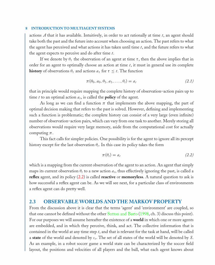
actions A that it has available. Intuitively, in order to act rationally at time t, an agent shouldtake both the past and the future into account when choosing an action. The past refers to whatthe agent has perceived and what actions it has taken until time t, and the future refers to whatthe agent expects to perceive and do after time t.
If we denote by θτ the observation of an agent at time τ , then the above implies that inorder for an agent to optimally choose an action at time t, it must in general use its completehistory of observations θτ and actions aτ for τ ≤ t. The function
π (θ0, a0, θ1, a1, . . . , θt) = at (2.1)
that in principle would require mapping the complete history of observation–action pairs up totime t to an optimal action at , is called the policy of the agent.
As long as we can find a function π that implements the above mapping, the part ofoptimal decision making that refers to the past is solved. However, defining and implementingsuch a function is problematic; the complete history can consist of a very large (even infinite)number of observation–action pairs, which can vary from one task to another. Merely storing allobservations would require very large memory, aside from the computational cost for actuallycomputing π .
This fact calls for simpler policies. One possibility is for the agent to ignore all its percepthistory except for the last observation θt . In this case its policy takes the form
π (θt) = at (2.2)
which is a mapping from the current observation of the agent to an action. An agent that simplymaps its current observation θt to a new action at , thus effectively ignoring the past, is called areflex agent, and its policy (2.2) is called reactive or memoryless. A natural question to ask ishow successful a reflex agent can be. As we will see next, for a particular class of environmentsa reflex agent can do pretty well.
2.3 OBSERVABLE WORLDS AND THE MARKOV PROPERTYFrom the discussion above it is clear that the terms ‘agent’ and ‘environment’ are coupled, sothat one cannot be defined without the other Sutton and Barto (1998, ch. 3) discuss this point).For our purposes we will assume hereafter the existence of a world in which one or more agentsare embedded, and in which they perceive, think, and act. The collective information that iscontained in the world at any time step t, and that is relevant for the task at hand, will be calleda state of the world and denoted by s t . The set of all states of the world will be denoted by S.As an example, in a robot soccer game a world state can be characterized by the soccer fieldlayout, the positions and velocities of all players and the ball, what each agent knows about

book MOBK077-Vlassis August 3, 2007 7:59
RATIONAL AGENTS 9
each other, and other parameters that are relevant to the decision making of the agents like theelapsed time since the game started, etc.
Depending on the nature of the problem, a world can be either discrete or continuous.A discrete world can be characterized by a finite number of states, like the possible boardconfigurations in a chess game. A continuous world can have infinitely many states, like thepossible configurations of a point robot that translates freely on the plane in which case S = IR2.Most of the existing AI techniques have been developed for discrete worlds, and this will beour main focus as well.
2.3.1 ObservabilityA fundamental property that characterizes a world from the point of view of an agent is relatedto the perception of the agent. We will say that the world is (fully) observable to an agent ifthe current observation θt of the agent completely reveals the current state of the world, that is,s t = θt . On the other hand, in a partially observable world the current observation θt of theagent provides only partial information about the current state s t in the form of a deterministicor stochastic observation model, for instance a conditional probability distribution p(s t|θt).The latter would imply that the current observation θt does not fully reveal the true worldstate, but to each state s t the agent assigns probability p(s t|θt) that s t is the true state (with0 ≤ p(s t|θt) ≤ 1 and
∑s t∈S p(s t|θt) = 1). Here we treat s t as a random variable that can take
all possible values in S. The stochastic coupling between s t and θt may alternatively be definedby an observation model in the form p(θt|s t), and a posterior state distribution p(s t|θt) can becomputed from a prior distribution p(s t) using the Bayes rule:
p(s t|θt) = p(θt|s t)p(s t)p(θt)
. (2.3)
Partial observability can in principle be attributed to two factors. First, it can be the resultof noise in the agent’s sensors. For example, due to sensor malfunction, the same state may‘generate’ different observations to the agent at different points in time. That is, every time theagent visits a particular state it may perceive something different. Second, partial observabilitycan be related to an inherent property of the environment referred to as perceptual aliasing:different states may produce identical observations to the agent at different time steps. In otherwords, two states may ‘look’ the same to an agent, although the states are different from eachother. For example, two identical doors along a corridor will look exactly the same to the eyesof a human or the camera of a mobile robot, no matter how accurate each sensor system is.
Partial observability is much harder to handle than full observability, and algorithms foroptimal decision making in a partially observable world can often become intractable. As we
book MOBK077-Vlassis August 3, 2007 7:59
10 INTRODUCTION TO MULTIAGENT SYSTEMS
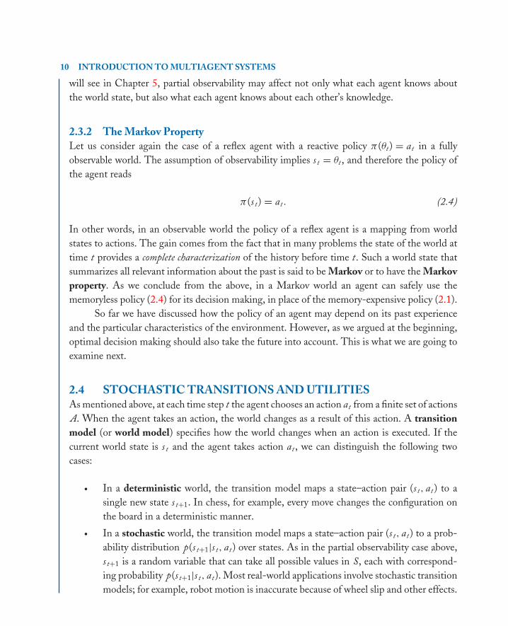
will see in Chapter 5, partial observability may affect not only what each agent knows aboutthe world state, but also what each agent knows about each other’s knowledge.
2.3.2 The Markov PropertyLet us consider again the case of a reflex agent with a reactive policy π (θt) = at in a fullyobservable world. The assumption of observability implies s t = θt , and therefore the policy ofthe agent reads
π (s t) = at . (2.4)
In other words, in an observable world the policy of a reflex agent is a mapping from worldstates to actions. The gain comes from the fact that in many problems the state of the world attime t provides a complete characterization of the history before time t. Such a world state thatsummarizes all relevant information about the past is said to be Markov or to have the Markovproperty. As we conclude from the above, in a Markov world an agent can safely use thememoryless policy (2.4) for its decision making, in place of the memory-expensive policy (2.1).
So far we have discussed how the policy of an agent may depend on its past experienceand the particular characteristics of the environment. However, as we argued at the beginning,optimal decision making should also take the future into account. This is what we are going toexamine next.
2.4 STOCHASTIC TRANSITIONS AND UTILITIESAs mentioned above, at each time step t the agent chooses an action at from a finite set of actionsA. When the agent takes an action, the world changes as a result of this action. A transitionmodel (or world model) specifies how the world changes when an action is executed. If thecurrent world state is s t and the agent takes action at , we can distinguish the following twocases:
� In a deterministic world, the transition model maps a state–action pair (s t, at) to asingle new state s t+1. In chess, for example, every move changes the configuration onthe board in a deterministic manner.
� In a stochastic world, the transition model maps a state–action pair (s t, at) to a prob-ability distribution p(s t+1|s t, at) over states. As in the partial observability case above,s t+1 is a random variable that can take all possible values in S, each with correspond-ing probability p(s t+1|s t, at). Most real-world applications involve stochastic transitionmodels; for example, robot motion is inaccurate because of wheel slip and other effects.

book MOBK077-Vlassis August 3, 2007 7:59
RATIONAL AGENTS 11
We saw in the previous section that sometimes partial observability can be attributed touncertainty in the perception of the agent. Here we see another example where uncertainty playsa role; namely, in the way the world changes when the agent executes an action. In a stochasticworld, the effects of the actions of the agent are not known a priori. Instead, there is a randomelement that decides how the world changes as a result of an action. Clearly, stochasticity inthe state transitions introduces an additional difficulty in the optimal decision making task ofthe agent.
2.4.1 From Goals to UtilitiesIn classical AI, a goal for a particular task is a desired state of the world. Accordingly, planningis defined as a search through the state space for an optimal path to the goal. When the world isdeterministic, planning comes down to a graph search problem for which a variety of methodsexist (Russell and Norvig, 2003, ch. 3).
In a stochastic world, however, planning cannot be done by simple graph search becausetransitions between states are nondeterministic. The agent must now take the uncertainty ofthe transitions into account when planning. To see how this can be realized, note that in adeterministic world an agent prefers by default a goal state to a non-goal state. More generally,an agent may hold preferences between any world states. For example, a soccer agent willmostly prefer to score a goal, will prefer less (but still a lot) to stand with the ball in front of anempty goal, and so on.
A way to formalize the notion of state preferences is by assigning to each state s a realnumber U (s ) that is called the utility of state s for that particular agent. Formally, for two statess and s ′ holds U (s ) > U (s ′) if and only if the agent prefers state s to state s ′, and U (s ) = U (s ′)if and only if the agent is indifferent between s and s ′. Intuitively, the utility of a state expressesthe ‘desirability’ of that state for the particular agent; the larger the utility of the state, the betterthe state is for that agent. In the discrete world of Fig. 2.1, for instance, an agent would preferstate d3 than state b2 or d2. Note that in a multiagent system, a state may be desirable to aparticular agent and at the same time be undesirable to an another agent; in soccer, for example,scoring is typically unpleasant to the opponent agents.
43 +12 −1−11 start
a b c d
FIGURE 2.1: A world with one desired (+1) and two undesired (−1) states

book MOBK077-Vlassis August 3, 2007 7:59
12 INTRODUCTION TO MULTIAGENT SYSTEMS
2.4.2 Decision Making in a Stochastic WorldEquipped with utilities, the question now is how an agent can effectively use them for itsdecision making. Let us assume that there is only one agent in the world, and the world isstochastic with transition model p(s t+1|s t, at). Suppose that the current state is s t , and the agentis pondering how to choose its action at . Let U (s ) be the utility function for the particularagent. Utility-based decision making is based on the premise that the optimal action a∗
t of theagent at state s t should maximize expected utility, that is,
a∗t = arg max
at∈A
∑
s t+1
p(s t+1|s t, at)U (s t+1) (2.5)
where we sum over all possible states s t+1 ∈ S the world may transition to, given that the currentstate is s t and the agent takes action at . In words, to see how good an action is, the agent hasto multiply the utility of each possible resulting state with the probability of actually reachingthis state, and sum up over all states. Then the agent must choose the action a∗
t that gives thehighest sum.
If each world state possesses a utility value, the agent can do the above calculations andcompute an optimal action for each possible state. This provides the agent with a policy thatmaps states to actions in an optimal sense (optimal with respect to the given utilities). Inparticular, given a set of optimal (that is, highest attainable) utilities U∗(s ) in a given task, thegreedy policy
π∗(s ) = arg maxa
∑
s ′p(s ′|s , a)U∗(s ′) (2.6)
is an optimal policy for the agent.There is an alternative and often useful way to characterize an optimal policy. For each
state s and each possible action a we can define an optimal action value or Q-value Q∗(s , a)that measures the ‘goodness’ of action a in state s for that agent. For the Q-values holdsU∗(s ) = maxa Q∗(s , a), while an optimal policy can be computed as
π∗(s ) = arg maxa
Q∗(s , a) (2.7)
which is a simpler formula than (2.6) that does not make use of a transition model. In Chapter 7we will see how we can compute optimal Q-values Q∗(s , a), and hence an optimal policy, in agiven task.
2.4.3 Example: A Toy WorldLet us close the chapter with an example, similar to the one used by Russell and Norvig (2003,ch. 21). Consider the world of Fig. 2.1 where in any state the agent can choose any one of

book MOBK077-Vlassis August 3, 2007 7:59
RATIONAL AGENTS 13
4 0.818 (→) 0.865 (→
→
) 0.911 (→) 0.953 (↓)3 0.782 (↑) 0.827 (↑) 0.907 (→) +12 0.547 (↑) −1 −10.492 (↑)1 0.480 (↑) 0.279 ( ) →( )0.410 (↑) 0.216
a b c d
FIGURE 2.2: Optimal utilities and an optimal policy of the agent
the actions {Up, Down, Left, Right }. We assume that the world is fully observable (the agentalways knows where it is), and stochastic in the following sense: every action of the agent toan intended direction succeeds with probability 0.8, but with probability 0.2 the agent ends upperpendicularly to the intended direction. Bumping on the border leaves the position of theagent unchanged. There are three terminal states, a desired one (the ‘goal’ state) with utility+1, and two undesired ones with utility −1. The initial position of the agent is a1.
We stress again that although the agent can perceive its own position and thus the stateof the world, it cannot predict the effects of its actions on the world. For example, if the agentis in state c2, it knows that it is in state c2. However, if it tries to move Up to state c3, it mayreach the intended state c3 (this will happen in 80% of the cases) but it may also reach state b2(in 10% of the cases) or state d2 (in the rest 10% of the cases).
Assume now that optimal utilities have been computed for all states, as shown in Fig. 2.2.Applying the principle of maximum expected utility, the agent computes that, for instance, instate b3 the optimal action is Up. Note that this is the only action that avoids an accidentaltransition to state b2. Similarly, by using (2.6) the agent can now compute an optimal actionfor every state, which gives the optimal policy shown in parentheses.
Note that, unlike path planning in a deterministic world that can be described as graphsearch, decision making in stochastic domains requires computing a complete policy that mapsstates to actions. Again, this is a consequence of the fact that the results of the actions of anagent are unpredictable. Only after the agent has executed its action it can observe the newstate of the world, from which it can select another action based on its precomputed policy.
2.5 NOTES AND FURTHER READINGWe have mainly followed Chapters 2, 16, and 17 of the book of Russell and Norvig (2003)which we strongly recommend for further reading. An illuminating discussion on the agent–environment interface and the Markov property can be found in Chapter 3 of the bookof Sutton and Barto (1998) which is another excellent text on agents and decision making.Bertsekas (2001) provides a more technical exposition. Spaan and Vlassis (2005) outline recentadvances in the topic of sequential decision making under partial observability.

book MOBK077-Vlassis August 3, 2007 7:59
14
book MOBK077-Vlassis August 3, 2007 7:59
15
C H A P T E R 3
Strategic Games
In this chapter we study the problem of multiagent decision making where a group of agentscoexist in an environment and take simultaneous decisions. We use game theory to analyzethe problem. In particular, we describe the model of a strategic game and we examine twofundamental solution concepts, iterated elimination of strictly dominated actions and Nashequilibrium.
3.1 GAME THEORYAs we saw in Chapter 2, an agent will typically be uncertain about the effects of its actions tothe environment, and it has to take this uncertainty into account in its decision making. In amultiagent system where many agents take decisions at the same time, an agent will also beuncertain about the decisions of the other participating agents. Clearly, what an agent shoulddo depends on what the other agents will do.
Multiagent decision making is the subject of game theory (Osborne and Rubinstein,1994). Although originally designed for modeling economical interactions, game theory hasdeveloped into an independent field with solid mathematical foundations and many applica-tions. The theory tries to understand the behavior of interacting agents under conditions ofuncertainty, and is based on two premises. First, that the participating agents are rational.Second, that they reason strategically, that is, they take into account the other agents’ decisionsin their decision making.
Depending on the way the agents choose their actions, there are different types of games.In a strategic game each agent chooses his1 strategy only once at the beginning of the game,and then all agents take their actions simultaneously. In an extensive game the agents areallowed to reconsider their plans during the game, and they may be imperfectly informedabout the actions played by the other agents. In this chapter we will only consider strategicgames.
1In this chapter we will use ‘he’ or ‘she’ to refer to an agent, following the convention in the literature(Osborne and Rubinstein, 1994, p. xiii).
book MOBK077-Vlassis August 3, 2007 7:59
16 INTRODUCTION TO MULTIAGENT SYSTEMS
3.2 STRATEGIC GAMESA strategic game, or game in normal form, is the simplest game-theoretic model of agents’interaction. It can be viewed as a multiagent extension of the decision-theoretic model of Chap-ter 2, and is characterized by the following elements:
� There are n > 1 agents in the world.� Each agent i can choose an action, or strategy, ai from his own action set Ai . The
tuple (a1, . . . , an) of individual actions is called a joint action or an action profile,and is denoted by a or (ai ). We will use the notation a−i to refer the actions of allagents except i , and (ai , a−i ) or [ai , a−i ] to refer to a joint action where agent i takes aparticular action ai .
� The game is ‘played’ on a fixed world state s (we are not concerned with state transitionshere). The state can be defined as consisting of the n agents, their action sets Ai , andtheir payoffs, as we explain next.
� Each agent i has his own action value function Q∗i (s , a) that measures the goodness of
the joint action a for the agent i . Note that each agent may assign different preferencesto different joint actions. Since s is fixed, we drop the symbol s and instead useui (a) ≡ Q∗
i (s , a), which is called the payoff function of agent i . We assume that thepayoff functions are predefined and fixed. (We will deal with the case of learning thepayoff functions in Chapter 7.)
� The state is fully observable to all agents. That is, all agents know (i) each other, (ii) theaction sets of each other, and (iii) the payoffs of each other. More strictly, the primitives(i)-(iii) of the game are common knowledge among agents. That is, all agents know(i)–(iii), they all know that they all know (i)–(iii), and so on to any depth. (We willdiscuss common knowledge in detail in Chapter 5.)
� Each agent chooses a single action; it is a single-shot game. Moreover, all agents choosetheir actions simultaneously and independently; no agent is informed of the decisionof any other agent prior to making his own decision.
In summary, in a strategic game each agent chooses a single action, and then he receivesa payoff that depends on the selected joint action. This joint action is called the outcome ofthe game. Although the payoff functions of the agents are common knowledge, an agent doesnot know in advance the action choices of the other agents. The best he can do is to try topredict the actions of the other agents. A solution to a game is a prediction of the outcome ofthe game using the assumption that all agents are rational and strategic.

book MOBK077-Vlassis August 3, 2007 7:59
STRATEGIC GAMES 17
Not confess ConfessNot confess 3, 3 0, 4
Confess 4, 0 1, 1
FIGURE 3.1: The prisoner’s dilemma
In the special case of two agents, a strategic game can be graphically represented bya payoff matrix, where the rows correspond to the actions of agent 1, the columns to theactions of agent 2, and each entry of the matrix contains the payoffs of the two agents forthe corresponding joint action. In Fig. 3.1 we show the payoff matrix of a classical game, theprisoner’s dilemma, whose story goes as follows:
Two suspects in a crime are independently interrogated. If they both confess, each willspend three years in prison. If only one confesses, he will run free while the other will spendfour years in prison. If neither confesses, each will spend one year in prison.
In this example each agent has two available actions, Not confess or Confess. Translatingthe above story into appropriate payoffs for the agents, we get in each entry of the matrix thepairs of numbers that are shown in Fig. 3.1 (note that a payoff is by definition a ‘reward’,whereas spending three years in prison is a ‘penalty’). For example, the entry (4, 0) indicatesthat if the first agent confesses and the second agent does not, then the first agent will getpayoff 4 and the second agent will get payoff 0.
In Fig. 3.2 we see two more examples of strategic games. The game in Fig. 3.2(a) isknown as ‘matching pennies’; each of two agents chooses either Head or Tail. If the choicesdiffer, agent 1 pays agent 2 a cent; if they are the same, agent 2 pays agent 1 a cent. Such agame is called strictly competitive or zero-sum because u1(a) + u2(a) = 0 for all a . The gamein Fig. 3.2(b) is played between two car drivers at a crossroad; each agent wants to cross first(and he will get payoff 1), but if they both cross they will crash (and get payoff −1). Such agame is called a coordination game (we will study coordination games in Chapter 4).
What does game theory predict that a rational agent will do in the above examples? Inthe next sections we will describe two fundamental solution concepts for strategic games.
Head TailHead 1,−1
1,−1Tail −1, 1−1, 1 −1, 1
Cross StopCross 1, 0Stop 0, 1 0, 0
(a) (b)
FIGURE 3.2: A strictly competitive game (a), and a coordination game (b)

book MOBK077-Vlassis August 3, 2007 7:59
18 INTRODUCTION TO MULTIAGENT SYSTEMS
3.3 ITERATED ELIMINATION OF DOMINATED ACTIONSThe first solution concept is based on the assumption that a rational agent will never choose asuboptimal action. With suboptimal we mean an action that, no matter what the other agentsdo, will always result in lower payoff for the agent than some other action. We formalize thisas follows:
Definition 3.1. We will say that an action ai of agent i is strictly dominated by another action a ′i
of agent i if
ui (a ′i , a−i ) > ui (ai , a−i ) (3.1)
for all actions a−i of the other agents.
In the above definition, ui (ai , a−i ) is the payoff the agent i receives if he takes action ai
while the other agents take a−i . In the prisoner’s dilemma, for example, Not confess is a strictlydominated action for agent 1; no matter what agent 2 does, the action Confess always givesagent 1 higher payoff than the action Not confess (4 as opposed to 3 if agent 2 does not confess,and 1 as opposed to 0 if agent 2 confesses). Similarly, Not confess is a strictly dominated actionfor agent 2.
Iterated elimination of strictly dominated actions (IESDA) is a solution techniquethat iteratively eliminates strictly dominated actions from all agents, until no more actions arestrictly dominated. It is solely based on the following two assumptions:
� A rational agent would never take a strictly dominated action.� It is common knowledge that all agents are rational.
As an example, we will apply IESDA to the prisoner’s dilemma. As we explained above,the action Not confess is strictly dominated by the action Confess for both agents. Let us startfrom agent 1 by eliminating the action Not confess from his action set. Then the game reduces toa single-row payoff matrix where the action of agent 1 is fixed (Confess ) and agent 2 can choosebetween Not confess and Confess. Since the latter gives higher payoff to agent 2 (4 as opposedto 3), agent 2 will prefer Confess to Not confess. Thus IESDA predicts that the outcome of theprisoner’s dilemma will be (Confess, Confess ).
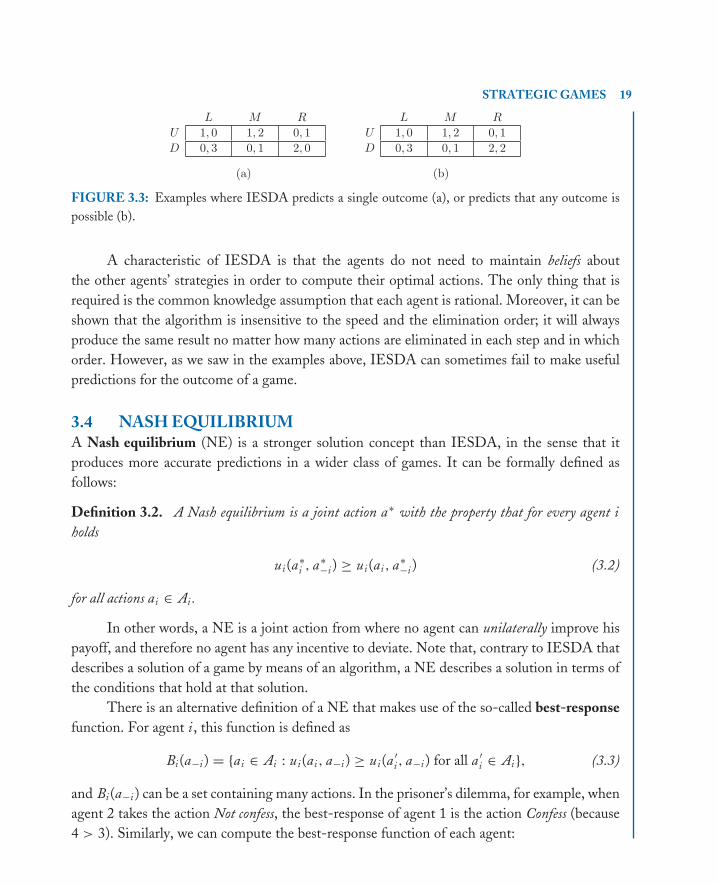
As another example consider the game of Fig. 3.3(a) where agent 1 has two actions Uand D and agent 2 has three actions L, M, and R. It is easy to verify that in this game IESDAwill predict the outcome (U , M) by first eliminating R (strictly dominated by M), then D, andfinally L. However, IESDA may sometimes produce very inaccurate predictions for a game,as in the two games of Fig. 3.2 and also in the game of Fig. 3.3(b) where no actions can beeliminated. In these games IESDA essentially predicts that any outcome is possible.
book MOBK077-Vlassis August 3, 2007 7:59
STRATEGIC GAMES 19
L M R
U 1, 0 1, 2 0, 1D 0, 3 0, 1 2, 0
L M R
U 1, 0 1, 2 0, 1D 0, 3 0, 1 2, 2
(a) (b)
FIGURE 3.3: Examples where IESDA predicts a single outcome (a), or predicts that any outcome ispossible (b).
A characteristic of IESDA is that the agents do not need to maintain beliefs aboutthe other agents’ strategies in order to compute their optimal actions. The only thing that isrequired is the common knowledge assumption that each agent is rational. Moreover, it can beshown that the algorithm is insensitive to the speed and the elimination order; it will alwaysproduce the same result no matter how many actions are eliminated in each step and in whichorder. However, as we saw in the examples above, IESDA can sometimes fail to make usefulpredictions for the outcome of a game.
3.4 NASH EQUILIBRIUMA Nash equilibrium (NE) is a stronger solution concept than IESDA, in the sense that itproduces more accurate predictions in a wider class of games. It can be formally defined asfollows:
Definition 3.2. A Nash equilibrium is a joint action a∗ with the property that for every agent iholds
ui (a∗i , a∗
−i ) ≥ ui (ai , a∗−i ) (3.2)
for all actions ai ∈ Ai .
In other words, a NE is a joint action from where no agent can unilaterally improve hispayoff, and therefore no agent has any incentive to deviate. Note that, contrary to IESDA thatdescribes a solution of a game by means of an algorithm, a NE describes a solution in terms ofthe conditions that hold at that solution.
There is an alternative definition of a NE that makes use of the so-called best-responsefunction. For agent i , this function is defined as
Bi (a−i ) = {ai ∈ Ai : ui (ai , a−i ) ≥ ui (a ′i , a−i ) for all a ′
i ∈ Ai}, (3.3)
and Bi (a−i ) can be a set containing many actions. In the prisoner’s dilemma, for example, whenagent 2 takes the action Not confess, the best-response of agent 1 is the action Confess (because4 > 3). Similarly, we can compute the best-response function of each agent:
book MOBK077-Vlassis August 3, 2007 7:59
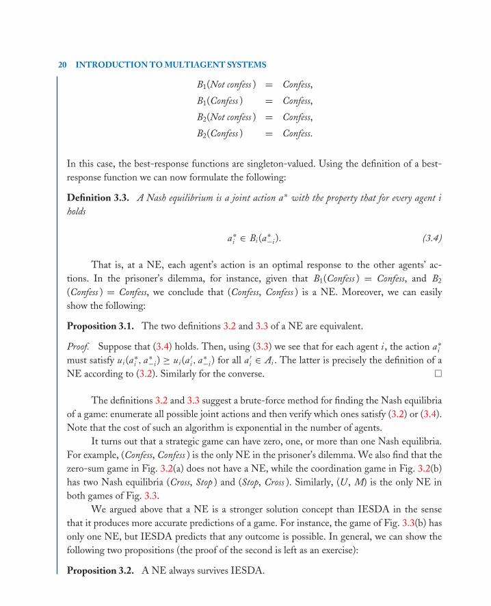
20 INTRODUCTION TO MULTIAGENT SYSTEMS
B1(Not confess ) = Confess,
B1(Confess ) = Confess,
B2(Not confess ) = Confess,
B2(Confess ) = Confess.
In this case, the best-response functions are singleton-valued. Using the definition of a best-response function we can now formulate the following:
Definition 3.3. A Nash equilibrium is a joint action a∗ with the property that for every agent iholds
a∗i ∈ Bi (a∗
−i ). (3.4)
That is, at a NE, each agent’s action is an optimal response to the other agents’ ac-tions. In the prisoner’s dilemma, for instance, given that B1(Confess ) = Confess, and B2
(Confess ) = Confess, we conclude that (Confess, Confess ) is a NE. Moreover, we can easilyshow the following:
Proposition 3.1. The two definitions 3.2 and 3.3 of a NE are equivalent.
Proof. Suppose that (3.4) holds. Then, using (3.3) we see that for each agent i , the action a∗i
must satisfy ui (a∗i , a∗
−i ) ≥ ui (a ′i , a∗
−i ) for all a ′i ∈ Ai . The latter is precisely the definition of a
NE according to (3.2). Similarly for the converse. �
The definitions 3.2 and 3.3 suggest a brute-force method for finding the Nash equilibriaof a game: enumerate all possible joint actions and then verify which ones satisfy (3.2) or (3.4).Note that the cost of such an algorithm is exponential in the number of agents.
It turns out that a strategic game can have zero, one, or more than one Nash equilibria.For example, (Confess, Confess ) is the only NE in the prisoner’s dilemma. We also find that thezero-sum game in Fig. 3.2(a) does not have a NE, while the coordination game in Fig. 3.2(b)has two Nash equilibria (Cross, Stop ) and (Stop, Cross ). Similarly, (U , M) is the only NE inboth games of Fig. 3.3.
We argued above that a NE is a stronger solution concept than IESDA in the sensethat it produces more accurate predictions of a game. For instance, the game of Fig. 3.3(b) hasonly one NE, but IESDA predicts that any outcome is possible. In general, we can show thefollowing two propositions (the proof of the second is left as an exercise):
Proposition 3.2. A NE always survives IESDA.
book MOBK077-Vlassis August 3, 2007 7:59
STRATEGIC GAMES 21
Proof. Let a∗ be a NE, and let us assume that a∗ does not survive IESDA. This means thatfor some agent i the component a∗
i of the action profile a∗ is strictly dominated by anotheraction ai of agent i . But then (3.1) implies that ui (ai , a∗
−i ) > ui (a∗i , a∗
−i ) which contradicts theDefinition 3.2 of a NE. �
Proposition 3.3. If IESDA eliminates all but a single joint action a , then a is the unique NEof the game.
Note also that in the prisoner’s dilemma, the joint action (Not confess, Not confess ) givesboth agents payoff 3, and thus it should have been the preferable choice. However, from thisjoint action each agent has an incentive to deviate, to be a ‘free rider’. Only if the agents hadmade an agreement in advance, and only if trust between them was common knowledge, wouldthey have opted for this non-equilibrium joint action which is optimal in the following sense:
Definition 3.4. A joint action a is Pareto optimal if there is no other joint action a ′ for whichui (a ′) ≥ ui (a) for each i and u j (a ′) > u j (a) for some j .
So far we have implicitly assumed that when the game is actually played, each agent iwill choose his action deterministically from his action set Ai . This is however not always true.In many cases there are good reasons for an agent to introduce randomness in his behavior; forinstance, to avoid being predictable when he repeatedly plays a zero-sum game. In these casesan agent i can choose actions ai according to some probability distribution:
Definition 3.5. A mixed strategy for an agent i is a probability distribution over his actionsai ∈ Ai .
In his celebrated theorem, Nash (1950) showed that a strategic game with a finite num-ber of agents and a finite number of actions always has an equilibrium in mixed strategies.Osborne and Rubinstein (1994, sec. 3.2) give several interpretations of such a mixed strat-egy Nash equilibrium. Porter et al. (2004) and von Stengel (2007) describe several algorithmsfor computing Nash equilibria, a problem whose complexity has been a long-standing is-sue (Papadimitriou, 2001).
3.5 NOTES AND FURTHER READINGThe book of von Neumann and Morgenstern (1944) and the half-page long article of Nash(1950) are classics in game theory. The book of Osborne and Rubinstein (1994) is the standardtextbook on game theory, and it is highly recommended. The book of Gibbons (1992) and thebook of Osborne (2003) offer a readable introduction to the field, with several applications.Russell and Norvig (2003, ch. 17) also include an introductory section on game theory. Thebook of Nisan et al. (2007) focuses on computational aspects of game theory.

book MOBK077-Vlassis August 3, 2007 7:59
22

book MOBK077-Vlassis August 3, 2007 7:59
23
C H A P T E R 4
Coordination
In this chapter we address the problem of multiagent coordination. We analyze the problemusing the framework of strategic games that we studied in Chapter 3, and we describe severalpractical techniques like social conventions, roles, and coordination graphs.
4.1 COORDINATION GAMESAs we argued in Chapter 1, decision making in a multiagent system should preferably be carriedout in a decentralized manner for reasons of efficiency and robustness. This additionally requiresdeveloping a coordination mechanism. In the case of collaborative agents, coordination ensuresthat the agents do not obstruct each other when taking actions, and that these actions servethe common goal of the team (for example, two teammate soccer robots must coordinate theiractions when deciding who should go for the ball). Informally, coordination can be regardedas the process by which the individual decisions of the agents result in good joint decisions forthe group.
Formally, we can model a coordination problem as a coordination game using the toolsof game theory, and solve it according to some solution concept, for instance Nash equilibrium.We have already seen an example in Fig. 3.2(b) of Chapter 3 of a strategic game where twocars meet at a crossroad and one driver should cross and the other one should stop. Thatgame has two Nash equilibria, (Cross, Stop) and (Stop, Cross). In the case of n collaborativeagents, all agents in the team share the same payoff function u1(a) = . . . = un(a) ≡ u(a) inthe corresponding coordination game. Figure 4.1 shows an example of a coordination game(played between two agents who want to go to the movies together) that also has two Nashequilibria. Generalizing from these two examples, we can formally define coordination as theprocess in which a group of agents choose a single Pareto optimal Nash equilibrium in a game.
Thriller ComedyThriller 1, 1 0, 0Comedy 0, 0 1, 1
FIGURE 4.1: A coordination game
book MOBK077-Vlassis August 3, 2007 7:59
24 INTRODUCTION TO MULTIAGENT SYSTEMS
In Chapter 3 we described a Nash equilibrium in terms of the conditions that hold at theequilibrium point, and disregarded the issue of how the agents can actually reach this point.Coordination is a more earthy concept, as it asks how the agents can actually agree on a singleequilibrium in a game that involves more than one equilibria. Reducing coordination to theproblem of equilibrium selection in a game allows for the application of existing techniquesfrom game theory (Harsanyi and Selten, 1988). In the rest of this chapter we will focus onsome simple coordination techniques that can be readily implemented in practical systems. Wewill throughout assume that the agents are collaborative (they share the same payoff function),and that they have perfect information about the game primitives (see Section 3.2). Also by‘equilibrium’ we will mean here ‘Pareto optimal Nash equilibrium’, unless otherwise stated.
4.2 SOCIAL CONVENTIONSAs we saw above, in order to solve a coordination problem, a group of agents are faced withthe problem of how to choose their actions in order to select the same equilibrium in a game.Clearly, there can be no recipe to tell the agents which equilibrium to choose in every possiblegame they may play in the future. Nevertheless, we can devise recipes that will instruct theagents on how to choose a single equilibrium in any game. Such a recipe will be able to guidethe agents in their action selection procedure.
A social convention (or social law) is such a recipe that places constraints on the possibleaction choices of the agents. It can be regarded as a rule that dictates how the agents shouldchoose their actions in a coordination game in order to reach an equilibrium. Moreover, giventhat the convention has been established and is common knowledge among agents, no agentcan benefit from not abiding by it.
Boutilier (1996) has proposed a general convention that achieves coordination in a largeclass of systems and is very easy to implement. The convention assumes a unique orderingscheme of joint actions that is common knowledge among agents. In a particular game, eachagent first computes all equilibria of the game, and then selects the first equilibrium accordingto this ordering scheme. For instance, a lexicographic ordering scheme can be used in whichthe agents are ordered first, and then the actions of each agent are ordered. In the coordinationgame of Fig. 4.1, for example, we can order the agents lexicographically by 1 � 2 (meaning thatagent 1 has ‘priority’ over agent 2), and the actions by Thriller � Comedy. The first equilibriumin the resulting ordering of joint actions is (Thriller, Thriller) and this will be the unanimouschoice of the agents. Given that a single equilibrium has been selected, each agent can thenchoose his individual action as the corresponding component of the selected equilibrium.
When the agents can perceive more aspects of the world state than just the primitivesof the game (actions and payoffs), one can think of more elaborate ordering schemes forcoordination. Consider the traffic game of Fig. 3.2(b), for example, as it is ‘played’ in the real

book MOBK077-Vlassis August 3, 2007 7:59
COORDINATION 25
world. Besides the game primitives, the state now also contains the relative orientation of thecars in the physical environment. If the state is fully observable by both agents (and this fact iscommon knowledge), then a simple convention is that the driver coming from the right willalways have priority over the other driver in the lexicographic ordering. If we also order theactions by Cross � Stop, then coordination by social conventions implies that the driver from theright will cross the road first. Similarly, if traffic lights are available, the established conventionis that the driver who sees the red light must stop.
When communication is available, we only need to impose an ordering i = 1, . . . , n ofthe agents that is common knowledge. Coordination can now be achieved by the followingalgorithm: Each agent i (except agent 1) waits until all previous agents 1, . . . , i − 1 in theordering have broadcast their chosen actions, and then agent i computes its component a∗
i ofan equilibrium that is consistent with the choices of the previous agents and broadcasts a∗
i toall agents that have not chosen an action yet. Note that here the fixed ordering of the agentstogether with the wait/send primitives result in a synchronized sequential execution order ofthe coordination algorithm.
4.3 ROLESCoordination by social conventions relies on the assumption that an agent can compute allequilibria in a game before choosing a single one. However, computing equilibria can beexpensive when the action sets of the agents are large, so it makes sense to try to reduce the sizeof the action sets first. Such a reduction can have computational advantages in terms of speed,but it can also simplify the equilibrium selection problem; in some cases the resulting subgamecontains only one equilibrium which is trivial to find.
A natural way to reduce the action sets of the agents is by assigning roles to the agents.Formally, a role can be regarded as a masking operator on the action set of an agent givena particular state. In practical terms, if an agent is assigned a role at a particular state, thensome of the agent’s actions are deactivated at this state. In soccer for example, an agent that iscurrently in the role of defender cannot attempt to Score.
A role can facilitate the solution of a coordination game by reducing it to a subgamewhere the equilibria are easier to find. For example, in Fig. 4.1, if agent 2 is assigned a role thatforbids him to select the action Thriller (say, he is under 12), then agent 1, assuming he knowsthe role of agent 2, can safely choose Comedy resulting in coordination. Note that there is onlyone equilibrium left in the subgame formed after removing the action Thriller from the actionset of agent 2.
In general, suppose that there are n available roles (not necessarily distinct), that the stateis fully observable to the agents, and that the following facts are common knowledge amongagents:

book MOBK077-Vlassis August 3, 2007 7:59
26 INTRODUCTION TO MULTIAGENT SYSTEMS
For each agent i in parallelI = {}.For each role j = 1, . . . , n
Compute the potential rij of agent i for role j.Broadcast rij to all agents.
EndWait until all ri′j , for j = 1, . . . , n, are received.For each role j = 1, . . . , n
Assign role j to agent i∗ = arg maxi′ /∈I{ri′j }.Add i∗ to I.
EndEnd
FIGURE 4.2: Communication-based greedy role assignment
� There is a fixed ordering {1, 2, . . . , n} of the roles. Role 1 must be assigned first,followed by role 2, etc.
� For each role there is a function that assigns to each agent a ‘potential’ that reflects howappropriate that agent is for the specific role, given the current state. For example, thepotential of a soccer robot for the role attacker can be given by its negative Euclideandistance to the ball.
� Each agent can be assigned only one role.
Then role assignment can be carried out, for instance, by a greedy algorithm in whicheach role (starting from role 1) is assigned to the agent that has the highest potential forthat role, and so on until all agents have been assigned a role. When communication is notavailable, each agent can run this algorithm identically and in parallel, assuming that each agentcan compute the potential of each other agent. When communication is available, an agentonly needs to compute its own potentials for the set of roles, and then broadcast them to therest of the agents. Next it can wait for all other potentials to arrive in order to compute theassignment of roles to agents as above. In the communication-based case, each agent needs tocompute O(n) (its own) potentials instead of O(n2) in the communication-free case, but this iscompensated by the total number O(n2) of potentials that need to be broadcast and processedby the agents. Figure 4.2 shows the greedy role assignment algorithm when communication isavailable.
4.4 COORDINATION GRAPHSAs mentioned above, roles can facilitate the solution of a coordination game by reducing theaction sets of the agents prior to computing the equilibria. However, computing equilibria in asubgame can still be a difficult task when the number of involved agents is large; recall that the

book MOBK077-Vlassis August 3, 2007 7:59
COORDINATION 27
joint action space is exponentially large in the number of agents. As roles reduce the size of theaction sets, we also need a method that reduces the number of agents involved in a coordinationgame.
Guestrin et al. (2002a) introduced the coordination graph as a framework for solvinglarge-scale coordination problems. A coordination graph allows for the decomposition of acoordination game into several smaller subgames that are easier to solve. Unlike roles where asingle subgame is formed by the reduced action sets of the agents, in this framework varioussubgames are formed, each typically involving a small number of agents.
In order for such a decomposition to apply, the main assumption is that the globalpayoff function u(a) can be written as a linear combination of k local payoff functions f j , forj = 1, . . . , k, each involving fewer agents. For example, suppose that there are n = 4 agents,and k = 3 local payoff functions, each involving two agents:
u(a) = f1(a1, a2) + f2(a1, a3) + f3(a3, a4). (4.1)
Here, for instance f2(a1, a3) involves only agents 1 and 3, with their actions a1 and a3. Such adecomposition can be graphically represented by a graph (hence the name), where each noderepresents an agent and each edge corresponds to a local payoff function. For example, thedecomposition (4.1) can be represented by the graph of Fig. 4.3.
Many practical problems can be modeled by such additively decomposable payoff func-tions. For example, in a computer network nearby servers may need to coordinate their actionsin order to optimize overall network traffic; in a firm with offices in different cities, geograph-ically nearby offices may need to coordinate their actions in order to maximize global sales; ina soccer team, nearby players may need to coordinate their actions in order to improve teamperformance; and so on.
Let us now see how this framework can be used for coordination. A solution to thecoordination problem is by definition a Pareto optimal Nash equilibrium in the correspondingstrategic game, that is, a joint action a∗ that maximizes u(a). We will describe two solution
2
1
3
4
f1 f2
f3
FIGURE 4.3: A coordination graph for a four-agent problem
book MOBK077-Vlassis August 3, 2007 7:59
28 INTRODUCTION TO MULTIAGENT SYSTEMS
methods: an exact one that is based on variable elimination, and an approximate one that isbased on message passing.
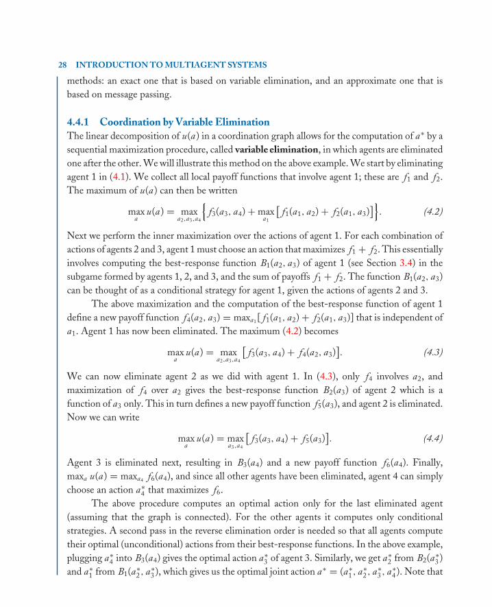
4.4.1 Coordination by Variable EliminationThe linear decomposition of u(a) in a coordination graph allows for the computation of a∗ by asequential maximization procedure, called variable elimination, in which agents are eliminatedone after the other. We will illustrate this method on the above example. We start by eliminatingagent 1 in (4.1). We collect all local payoff functions that involve agent 1; these are f1 and f2.The maximum of u(a) can then be written
maxa
u(a) = maxa2,a3,a4
{f3(a3, a4) + max
a1
[f1(a1, a2) + f2(a1, a3)
]}. (4.2)
Next we perform the inner maximization over the actions of agent 1. For each combination ofactions of agents 2 and 3, agent 1 must choose an action that maximizes f1 + f2. This essentiallyinvolves computing the best-response function B1(a2, a3) of agent 1 (see Section 3.4) in thesubgame formed by agents 1, 2, and 3, and the sum of payoffs f1 + f2. The function B1(a2, a3)can be thought of as a conditional strategy for agent 1, given the actions of agents 2 and 3.
The above maximization and the computation of the best-response function of agent 1define a new payoff function f4(a2, a3) = maxa1 [ f1(a1, a2) + f2(a1, a3)] that is independent ofa1. Agent 1 has now been eliminated. The maximum (4.2) becomes
maxa
u(a) = maxa2,a3,a4
[f3(a3, a4) + f4(a2, a3)
]. (4.3)
We can now eliminate agent 2 as we did with agent 1. In (4.3), only f4 involves a2, andmaximization of f4 over a2 gives the best-response function B2(a3) of agent 2 which is afunction of a3 only. This in turn defines a new payoff function f5(a3), and agent 2 is eliminated.Now we can write
maxa
u(a) = maxa3,a4
[f3(a3, a4) + f5(a3)
]. (4.4)
Agent 3 is eliminated next, resulting in B3(a4) and a new payoff function f6(a4). Finally,maxa u(a) = maxa4 f6(a4), and since all other agents have been eliminated, agent 4 can simplychoose an action a∗
4 that maximizes f6.The above procedure computes an optimal action only for the last eliminated agent
(assuming that the graph is connected). For the other agents it computes only conditionalstrategies. A second pass in the reverse elimination order is needed so that all agents computetheir optimal (unconditional) actions from their best-response functions. In the above example,plugging a∗
4 into B3(a4) gives the optimal action a∗3 of agent 3. Similarly, we get a∗
2 from B2(a∗3 )
and a∗1 from B1(a∗
2 , a∗3 ), which gives us the optimal joint action a∗ = (a∗
1 , a∗2 , a∗
3 , a∗4 ). Note that
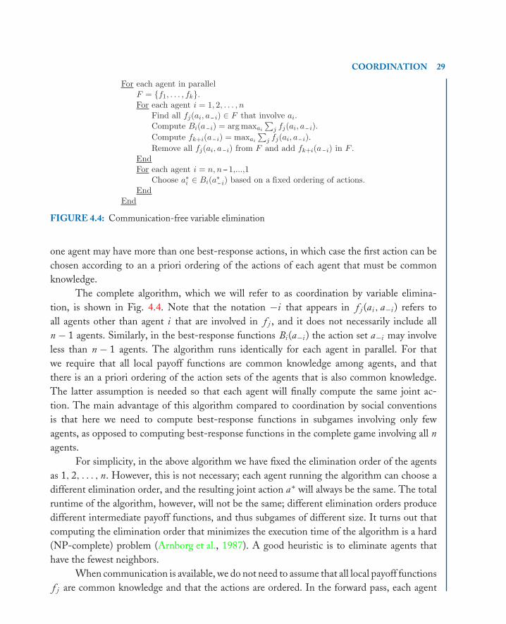
book MOBK077-Vlassis August 3, 2007 7:59
COORDINATION 29
For each agent in parallelF = {f1, . . . , fk}.For each agent i = 1, 2, . . . , n
Find all fj(ai, a− i) ∈ F that involve ai.Compute Bi(a− i) = arg maxai
∑j fj(ai, a− i).
Compute fk+i(a− i) = maxai∑
j fj(ai, a− i).Remove all fj(ai, a− i a− i) from F and add fk+i( ) in F .
EndFor each agent i = n, n− 1,...,1
Choose a∗i ∈ Bi(a∗− i) based on a fixed ordering of actions.End
End
FIGURE 4.4: Communication-free variable elimination
one agent may have more than one best-response actions, in which case the first action can bechosen according to an a priori ordering of the actions of each agent that must be commonknowledge.
The complete algorithm, which we will refer to as coordination by variable elimina-tion, is shown in Fig. 4.4. Note that the notation −i that appears in f j (ai , a−i ) refers toall agents other than agent i that are involved in f j , and it does not necessarily include alln − 1 agents. Similarly, in the best-response functions Bi (a−i ) the action set a−i may involveless than n − 1 agents. The algorithm runs identically for each agent in parallel. For thatwe require that all local payoff functions are common knowledge among agents, and thatthere is an a priori ordering of the action sets of the agents that is also common knowledge.The latter assumption is needed so that each agent will finally compute the same joint ac-tion. The main advantage of this algorithm compared to coordination by social conventionsis that here we need to compute best-response functions in subgames involving only fewagents, as opposed to computing best-response functions in the complete game involving all nagents.
For simplicity, in the above algorithm we have fixed the elimination order of the agentsas 1, 2, . . . , n. However, this is not necessary; each agent running the algorithm can choose adifferent elimination order, and the resulting joint action a∗ will always be the same. The totalruntime of the algorithm, however, will not be the same; different elimination orders producedifferent intermediate payoff functions, and thus subgames of different size. It turns out thatcomputing the elimination order that minimizes the execution time of the algorithm is a hard(NP-complete) problem (Arnborg et al., 1987). A good heuristic is to eliminate agents thathave the fewest neighbors.
When communication is available, we do not need to assume that all local payoff functionsf j are common knowledge and that the actions are ordered. In the forward pass, each agent

book MOBK077-Vlassis August 3, 2007 7:59
30 INTRODUCTION TO MULTIAGENT SYSTEMS
can maintain in its local memory the payoff functions that involve only this agent. The initialdistribution of payoff functions to the agents can be done as follows: agent 1 in the eliminationorder takes all payoff functions that involve this agent, agent 2 takes all functions that involvethis agent and are not distributed to agent 1, and so on, until no more payoff functions are left.When an agent computes its best-response function and generates a new payoff function, theagent can broadcast this function to the other agents involved in it. In fact, the agent needsto send the payoff function only to the first non-eliminated agent whose action appears in thedomain of this function. Similarly, in the backward pass an agent can wait for the optimalactions of the other agents (unless it is the last eliminated agent), then choose any actionfrom its best-response action set, and finally broadcast this action to all agents that need it intheir best-response functions. Figure 4.5 shows the communication-based version of variableelimination.
A crucial difference between the algorithms of Figs. 4.4 and 4.5 is that in thecommunication-based case the elimination order of the agents must be fixed a priori andit must be common knowledge among the agents. In terms of complexity, the forward passis slightly slower than in the communication-free case, because here the generated payoffsneed to be communicated to the other involved agents. On the other hand, when communi-cation is available, the backward pass can be fully asynchronous. One can also think of asyn-chronous versions of the forward pass in which many agents are simultaneously eliminated. Thiswould require some additional book-keeping for storing the pairwise dependencies betweenagents.
For each agent i in parallelIf i �= 1
Wait until agent i − 1 sends OK.EndLet fj(ai, ) be all local payoff functions (initial and communicated) thatinvolve agent i.Compute Bi( ) = arg maxai
∑j fj(ai, ).
Compute f∗( ) = maxai∑
j fj(ai, ).Send f∗(a− i
a− i
a− i
a− i
a− i
a− i
) to agent j = min{i + 1, . . . , n}, j ∈ − i.If i �= n
Send OK to agent i + 1.Wait until all a∗− i are received.
EndChoose any a∗i ∈ Bi(a∗− i).Broadcast a∗i to all agents j such that ai ∈ domain(Bj).
End
FIGURE 4.5: Communication-based variable elimination
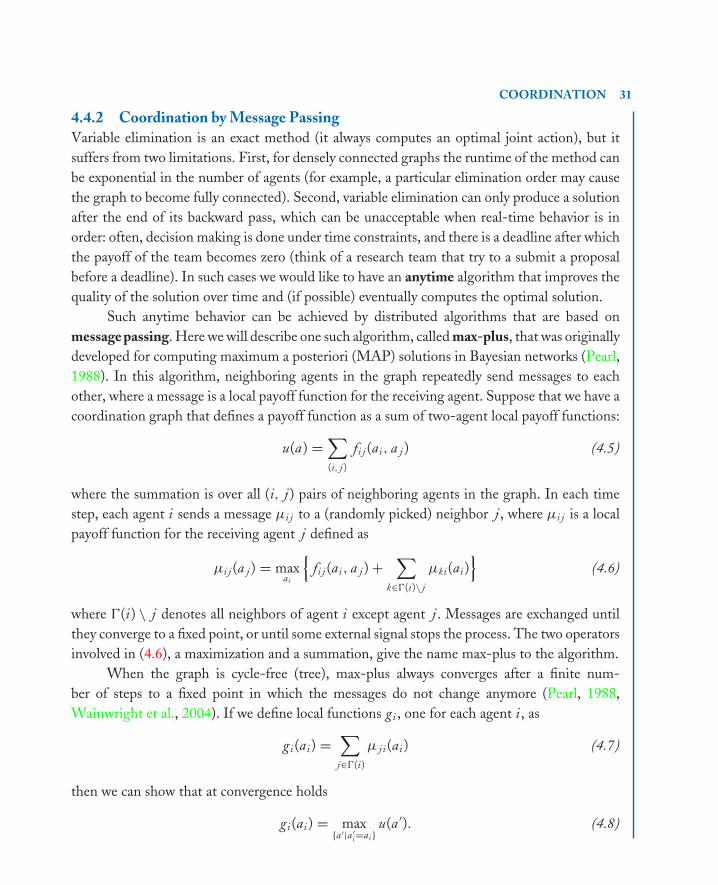
book MOBK077-Vlassis August 3, 2007 7:59
COORDINATION 31
4.4.2 Coordination by Message PassingVariable elimination is an exact method (it always computes an optimal joint action), but itsuffers from two limitations. First, for densely connected graphs the runtime of the method canbe exponential in the number of agents (for example, a particular elimination order may causethe graph to become fully connected). Second, variable elimination can only produce a solutionafter the end of its backward pass, which can be unacceptable when real-time behavior is inorder: often, decision making is done under time constraints, and there is a deadline after whichthe payoff of the team becomes zero (think of a research team that try to a submit a proposalbefore a deadline). In such cases we would like to have an anytime algorithm that improves thequality of the solution over time and (if possible) eventually computes the optimal solution.
Such anytime behavior can be achieved by distributed algorithms that are based onmessage passing. Here we will describe one such algorithm, called max-plus, that was originallydeveloped for computing maximum a posteriori (MAP) solutions in Bayesian networks (Pearl,1988). In this algorithm, neighboring agents in the graph repeatedly send messages to eachother, where a message is a local payoff function for the receiving agent. Suppose that we have acoordination graph that defines a payoff function as a sum of two-agent local payoff functions:
u(a) =∑
(i, j )
fi j (ai , a j ) (4.5)
where the summation is over all (i, j ) pairs of neighboring agents in the graph. In each timestep, each agent i sends a message µi j to a (randomly picked) neighbor j , where µi j is a localpayoff function for the receiving agent j defined as
µi j (a j ) = maxai
{fi j (ai , a j ) +
∑
k∈�(i)\ j
µki (ai )}
(4.6)
where �(i) \ j denotes all neighbors of agent i except agent j . Messages are exchanged untilthey converge to a fixed point, or until some external signal stops the process. The two operatorsinvolved in (4.6), a maximization and a summation, give the name max-plus to the algorithm.
When the graph is cycle-free (tree), max-plus always converges after a finite num-ber of steps to a fixed point in which the messages do not change anymore (Pearl, 1988,Wainwright et al., 2004). If we define local functions gi , one for each agent i , as
gi (ai ) =∑
j∈�(i)
µ j i (ai ) (4.7)
then we can show that at convergence holds
gi (ai ) = max{a ′|a ′
i =ai }u(a ′). (4.8)

book MOBK077-Vlassis August 3, 2007 7:59
32 INTRODUCTION TO MULTIAGENT SYSTEMS
If each agent locally computes
a∗i = arg max
ai
gi (ai ) (4.9)
and each optimal action a∗i is unique (for all i), then at convergence the globally optimal
action a∗ = arg maxa u(a) is also unique and has elements a∗ = (a∗i ) computed by only local
optimizations (each agent maximizes gi (ai ) separately). If the local a∗i are not unique, an
optimal joint action can still be computed by dynamic programming (Wainwright et al., 2004,sec. 3.1). Hence, max-plus allows the decomposition of a difficult global optimization problem(a∗ = arg maxa u(a)) into a set of local optimization problems (4.9) that are much easier tosolve.
When the graph contains cycles, there are no guarantees that max-plus will converge,nor that the local maximizers a∗
i from (4.9) will comprise a global maximum at any time step.However, max-plus can still be used as an approximate coordination algorithm, that producesvery good results in practice, much faster than variable elimination (Kok and Vlassis, 2006).
Max-plus is effective and simple to implement, but it comes with few performanceguarantees in general graphs. Other algorithms exist, based on branch and bound or hillclimbing, that can provably converge to the optimal solution (Modi et al., 2005), or to ak-optimal solution in which no subset of k or fewer agents can jointly improve the globalpayoff (Pearce and Tambe, 2007, Zhang et al., 2005).
4.5 NOTES AND FURTHER READINGMultiagent coordination has its roots in decentralized optimal control methods (Sandell et al.,1978). Early AI approaches to multiagent coordination are the ‘contract net protocol’ of Smith(1980) where tasks are dynamically distributed among agents using a bidding mechanism(see also Chapter 6), and the ‘partial global planning’ algorithm of Durfee and Lesser (1987)and Decker and Lesser (1995) in which agents exchange and refine local plans in order toreach a common goal. Jennings (1996) gives an overview of early coordination techniques indistributed AI. The framework of ‘joint intentions’ of Cohen and Levesque (1991) provides aformal characterization of multiagent coordination through a model of joint beliefs and inten-tions of the agents. Social conventions were introduced by Shoham and Tennenholtz (1992),as constraints on the set of allowed actions of a single agent at a given state (similar to thedefinition of roles in Section 4.3). Boutilier (1996) extended the definition to include alsoconstraints on the joint action choices of a group of agents, and proposed the idea of coor-dination by lexicographic ordering. The greedy algorithm for role assignment was proposedby Castelpietra et al. (2000). Gmytrasiewicz and Durfee (2001) analyze coordination and com-munication in a setting where the agents model the knowledge of each other recursively (see

book MOBK077-Vlassis August 3, 2007 7:59
COORDINATION 33
also Chapter 5). Coordination graphs are due to Guestrin et al. (2002a) who suggested the useof variable elimination for coordination. The max-plus algorithm on coordination graphs wassuggested by Vlassis et al. (2004). Coordination on a coordination graph is essentially identicalto a distributed constraint optimization problem (DCOP) (Modi et al., 2005, Yokoo, 2000), aparticular version of constraint processing (Dechter, 2003).

book MOBK077-Vlassis August 3, 2007 7:59
34
book MOBK077-Vlassis August 3, 2007 7:59
35
C H A P T E R 5
Partial Observability
In the previous chapters we assumed that the world state is fully observable to the agents. Herewe relax this assumption and examine the case where parts of the state are hidden to the agents.In such a partially observable world an agent must always reason about his knowledge, and theknowledge of the others, prior to making decisions. We formalize the notions of knowledgeand common knowledge in such domains, and describe the model of a Bayesian game formultiagent decision making under partial observability.
5.1 THINKING INTERACTIVELYIn order to act rationally, an agent must always reflect on what he knows about the currentworld state. As we saw in Chapter 2, if the state is fully observable, an agent can do prettywell without extensive deliberation. If the state is partially observable, however, the agentmust first consider carefully what he knows and what he does not know before choosing anaction.
In a multiagent system, partial observability forces a rational agent to think interactively,that is, to take into account the knowledge of the other agents in his decision making. Inaddition, an agent must consider what the other agents know about him, and also what theyknow about his knowledge. In the previous chapters we have often used the term commonknowledge to refer to something that every agent knows, that every agent knows that everyother agent knows, and so on. In this chapter we will define knowledge and common knowledgemore formally, and illustrate some of their implications through examples.
Partial observability may have various consequences to the decision making of the agents.For instance, optimal planning under partial observability can be a hard problem even in thesingle-agent case (Papadimitriou and Tsitsiklis, 1987). In the multiagent case, optimal planningunder partial observability is provably intractable (Bernstein et al., 2002). The latter is due tothe fact that, as stated above, each agent must take into account the knowledge of each otheragent in its decision making, which can significantly increase the complexity of the problem.Later in this chapter we will see how the model of a Bayesian game can be used for multiagentdecision making under partial observability.

book MOBK077-Vlassis August 3, 2007 7:59
36 INTRODUCTION TO MULTIAGENT SYSTEMS
5.2 INFORMATION AND KNOWLEDGEIn this section we will illustrate the concepts of information and common knowledge by meansof a classical puzzle, the puzzle of the hats:
Three agents (say, girls) are sitting around a table, each wearing a hat. A hat can be eitherred or white, but suppose that all agents are wearing red hats. Each agent can see the hatof the other two agents, but she does not know the color of her own hat. A person whoobserves all three agents asks them in turn whether they know the color of their hats. Eachagent replies negatively. Then the person announces ‘At least one of you is wearing a redhat’, and then asks them again in turn. Agent 1 says No. Agent 2 also says No. But when heasks agent 3, she says Yes.
How is it possible that agent 3 can finally figure out the color of her hat? Before theannouncement that at least one of them is wearing a red hat, no agent is able to tell her hatcolor. What changes then after the announcement? Seemingly the announcement does notreveal anything new; each agent already knows that there is at least one red hat because she cansee the red hats of the other two agents.
Given that everyone has heard that there is at least one red hat, agent 3 can tell her hatcolor by reasoning as follows: ‘Agent’s 1 No implies that either me or agent 2 is wearing a redhat. Agent 2 knows this, so if my hat had been white, agent 2 would have said Yes. But agent 2said No, so my hat must be red.’
Although each agent already knows (by perception) the fact that at least one agent iswearing a red hat, the key point is that the public announcement of the person makes thisfact common knowledge among the agents. (Implicitly we have also assumed that it is commonknowledge that each agent can see and hear well, and that she can reason rationally.) The puzzleis instructive as it demonstrates the implications of interactive reasoning and the strength ofthe common knowledge assumption.
Let us now try to formalize some of the concepts that appear in the puzzle. The startingpoint is that the world state is partially observable to the agents. Recall that in a partiallyobservable world the perception of an agent provides only partial information about the truestate by means of a deterministic or stochastic observation model (see Section 2.3). In the puzzleof the hats this model is a set-partition deterministic model, as we will see next.
Let S be the set of all states and s ∈ S be the current (true) state of the world. We assumethat the perception of an agent i provides information about the state s through an informationfunction Pi : S �→ 2S that maps s to Pi (s ), a nonempty subset of S called the informationset of agent i in state s . The interpretation of the information set is that when the true stateis s , agent i thinks that any state in Pi (s ) can be the true state. The set Pi (s ) will always

book MOBK077-Vlassis August 3, 2007 7:59
PARTIAL OBSERVABILITY 37
World statesa b c d e f g h
1 R R R R W W W WAgents 2 R R W W R R W W
3 R W R W R W R W
FIGURE 5.1: The eight world states in the puzzle of the hats
contain s , but essentially this is the only thing that agent i knows about the true state. In thecase of multiple agents, each agent can have a different information function.
In the puzzle of the hats, a state is a three-component vector containing the col-ors of the hats. Let R and W denote red and white. There are in total eight states S ={a, b, c , d , e , f, g , h}, as shown in Fig. 5.1. By assumption, the true state is s = a . From thesetup of the puzzle we know that the state is partially observable to each agent; only two ofthe three hat colors are directly perceivable by each agent. In other words, in any state s theinformation set of each agent contains two equiprobable states, those in which the only dif-ference is in her own hat color. For instance, in state s = a the information set of agent 2 isP2(s ) = {a, c }, a two-state subset of S.
As we mentioned above, the information set Pi (s ) of an agent i contains those states in Sthat agent i considers possible if the true state is s . In general, we assume that the informationfunction of an agent divides the state space into a collection of mutually disjoint subsets, calledcells, that together form a partition Pi of S. The information set Pi (s ) for agent i in truestate s is exactly that cell of Pi that contains s , while the union of all cells in Pi is S.
Based on the information functions, we can compute the partitions of the agents in thepuzzle of the hats:
P t1 = {{a, e }, {b, f }, {c , g}, {d , h}} (5.1)
P t2 = {{a, c }, {b, d}, {e , g}, { f, h}} (5.2)
P t3 = {{a, b}, {c , d}, {e , f }, {g , h}} (5.3)
where t refers to the time step before any announcement took place. Clearly, in the true states = a = RRR no agent knows her hat color, since the corresponding cell of each partitioncontains two equiprobable states. Thus, agent 1 considers a and e possible, agent 2 considers aand c possible, and agent 3 considers a and b possible. (Note again that we know that the truestate is a but the agents in our puzzle do not.)
Now we make the additional assumption that all partitions are common knowledgeamong the agents. In the case of homogeneous agents, for instance, this is not an unrealisticassumption; typically each agent will be aware of the perception capabilities of each other. Inthe puzzle of the hats, for example, it is reasonable to assume that all agents can see and hear

book MOBK077-Vlassis August 3, 2007 7:59
38 INTRODUCTION TO MULTIAGENT SYSTEMS
well and that they are all rational. Then, simply the positioning of the agents around the tablemakes the above partitions common knowledge.
If the partitions are common knowledge, then in state a agent 1 thinks that agent 2 maythink that agent 3 might think that h = WWW is possible! Why is that? Note from (5.1) thatin state a agent 1 thinks that either a or e could be the true state. But if e is the true state, thenfrom (5.2) we see that agent 2 may consider g to be the true state. But then we see from (5.3)that agent 3 may consider h to be the true state. Note how the above analytical frameworkallows for a fairly straightforward formulation of otherwise complicated statements.
Now the announcement of the person reveals that the true state is not h . This automati-cally changes the partitions of the agents:
P t+11 = {{a, e }, {b, f }, {c , g}, {d}, {h}}
P t+12 = {{a, c }, {b, d}, {e , g}, { f }, {h}}
P t+13 = {{a, b}, {c , d}, {e , f }, {g}, {h}}.
(5.4)
Note that h has been disambiguated from d , f , and g , in the three partitions. The person thenasks each agent in turn whether she knows the color of her hat. Agent 1 says No. In which casewould agent 1 have said Yes? As we see from the above partitions, only in state d would agent 1have known her hat color. But the true state is a , and in this state agent 1 still considers epossible.
The reply of agent 1 eliminates state d from the set of candidate states. This results in arefinement of the partitions of agents 2 and 3:
P t+21 = {{a, e }, {b, f }, {c , g}, {d}, {h}}
P t+22 = {{a, c }, {b}, {d}, {e , g}, { f }, {h}}
P t+23 = {{a, b}, {c }, {d}, {e , f }, {g}, {h}}.
(5.5)
Next agent 2 is asked. From her partition P t+22 we see that she would have known her
hat color only in state b or f (d and h are already ruled out by the previous announcements).However, in the true state a agent 2 still considers c possible, therefore she replies negatively.Her reply excludes b and f from the set of candidate states, resulting in a further refinementof the partitions of agent 1 and 3:
P t+31 = {{a, e }, {b}, { f }, {c , g}, {d}, {h}}
P t+32 = {{a, c }, {b}, {d}, {e , g}, { f }, {h}}
P t+33 = {{a}, {b}, {c }, {d}, {e }, { f }, {g}, {h}}.
(5.6)
The partition of agent 3 now contains only singleton cells, thus agent 3 can now tell her hatcolor. Note that agents 1 and 2 still cannot tell their hat colors. In fact, they will be unable to tell
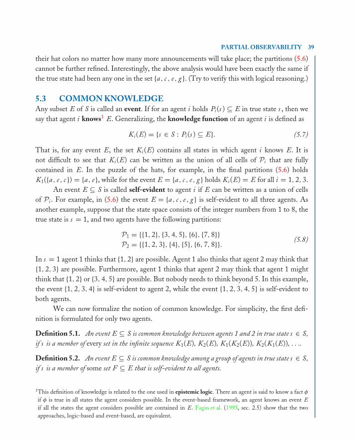
book MOBK077-Vlassis August 3, 2007 7:59
PARTIAL OBSERVABILITY 39
their hat colors no matter how many more announcements will take place; the partitions (5.6)cannot be further refined. Interestingly, the above analysis would have been exactly the same ifthe true state had been any one in the set {a, c , e , g}. (Try to verify this with logical reasoning.)
5.3 COMMON KNOWLEDGEAny subset E of S is called an event. If for an agent i holds Pi (s ) ⊆ E in true state s , then wesay that agent i knows1 E. Generalizing, the knowledge function of an agent i is defined as
Ki (E) = {s ∈ S : Pi (s ) ⊆ E}. (5.7)
That is, for any event E, the set Ki (E) contains all states in which agent i knows E. It isnot difficult to see that Ki (E) can be written as the union of all cells of Pi that are fullycontained in E. In the puzzle of the hats, for example, in the final partitions (5.6) holdsK1({a, e , c }) = {a, e }, while for the event E = {a, c , e , g} holds Ki (E) = E for all i = 1, 2, 3.
An event E ⊆ S is called self-evident to agent i if E can be written as a union of cellsof Pi . For example, in (5.6) the event E = {a, c , e , g} is self-evident to all three agents. Asanother example, suppose that the state space consists of the integer numbers from 1 to 8, thetrue state is s = 1, and two agents have the following partitions:
P1 = {{1, 2}, {3, 4, 5}, {6}, {7, 8}}P2 = {{1, 2, 3}, {4}, {5}, {6, 7, 8}}. (5.8)
In s = 1 agent 1 thinks that {1, 2} are possible. Agent 1 also thinks that agent 2 may think that{1, 2, 3} are possible. Furthermore, agent 1 thinks that agent 2 may think that agent 1 mightthink that {1, 2} or {3, 4, 5} are possible. But nobody needs to think beyond 5. In this example,the event {1, 2, 3, 4} is self-evident to agent 2, while the event {1, 2, 3, 4, 5} is self-evident toboth agents.
We can now formalize the notion of common knowledge. For simplicity, the first defi-nition is formulated for only two agents.
Definition 5.1. An event E ⊆ S is common knowledge between agents 1 and 2 in true state s ∈ S,if s is a member of every set in the infinite sequence K1(E), K2(E), K1(K2(E)), K2(K1(E)), . . ..
Definition 5.2. An event E ⊆ S is common knowledge among a group of agents in true state s ∈ S,if s is a member of some set F ⊆ E that is self-evident to all agents.
1This definition of knowledge is related to the one used in epistemic logic. There an agent is said to know a fact φ
if φ is true in all states the agent considers possible. In the event-based framework, an agent knows an event Eif all the states the agent considers possible are contained in E. Fagin et al. (1995, sec. 2.5) show that the twoapproaches, logic-based and event-based, are equivalent.

book MOBK077-Vlassis August 3, 2007 7:59
40 INTRODUCTION TO MULTIAGENT SYSTEMS
It turns out that the two definitions are equivalent (Osborne and Rubinstein, 1994,prop. 74.2). However, the second definition is much easier to apply; it only requires computingself-evident sets that are unions of partition cells and thus easy to find. For instance, in the aboveexample the event E = {1, 2, 3, 4, 5} is common knowledge between the two agents because Eis self-evident to both of them and the true state s = 1 belongs to E. Similarly, in the puzzleof the hats, in the final partitions (5.6), and with true state s = a , the event E = {a, c , e , g} iscommon knowledge among all three agents.
5.4 PARTIAL OBSERVABILITY AND ACTIONSSo far we have discussed how the observations of the agents are related to the world statesthrough the information functions, and what it means to say that an event is common knowledgeamong a group of agents. In this section we describe a framework that allows the agents to takerational decisions under partial observability.
Let us consider the puzzle of the hats again, and in particular the time step after the publicannouncement of the person. Below we identify the primitives of the multiagent interaction atthat step that are relevant for the decision making of the agents.
5.4.1 States and ObservationsThe true state is s = a = RRR and it is partially observable to the agents: each agent i receivesan observation θi ∈ �i that provides information about s via the information function Pi .(In the previous sections of this chapter the observations θi were not explicit; here we makethem explicit by associating each information set Pi (s ) with a corresponding observation θi .)For example, at s = RRR agent 1 observes θ1 = RR, meaning that she sees the two red hatsof agents 2 and 3, where θ1 is a member of the set �1 = {RR, RW, WR, WW} (all possibleobservations of agent 1). The profile of the individual observations of all agents (θi ) defines thejoint observation θ .
5.4.2 Observation ModelThe partition model associates with each observation θi of agent i a single information set Pi (s )that is a subset of the state space. For instance, θ1 = RR is associated with the information setP1(s ) = {a, e }. In this problem each observation is a deterministic function of the state: theobservation of each agent at each state is fully determined by the setup of the problem (theposition of a girl around the table). As we mentioned in Section 2.3, more general observationmodels can be defined in which the coupling between states and observations is stochastic.For instance, an observation model could define a joint probability distribution p(s , θ ) over
book MOBK077-Vlassis August 3, 2007 7:59
PARTIAL OBSERVABILITY 41
states and joint observations, from which various other quantities can be computed, like p(θ )or p(θ |s ), by using the laws of probability theory.2
5.4.3 Actions and PoliciesIn the puzzle of the hats each agent replies Yes or No to the question of the person ‘Do youknow your hat color?’. Such a reply can be regarded as an action taken by the agent given hercurrent information. For example, in the final partitions of (5.6), agent 1 will reply No givenher information set {a, e } and agent 3 will reply Yes given her information set {a}. In general, inmultiagent decision making under partial observability, the policy of each agent i is a mappingπi : �i �→ Ai from individual observations θi to individual actions ai = πi (θi ). (Recall thatthis was the definition of a memoryless policy of a reflex agent in Section 2.2.) The profile ofindividual policies (πi ) defines the joint policy π .
5.4.4 PayoffsIn the puzzle of the hats the agents reply truthfully to the questions of the person. Although wehave not explicitly defined a payoff function in this problem, we can think of an implicit payofffunction that the agents maximize, in which, say, truthfulness is highly valued. In general,multiagent decision making requires defining an explicit payoff function Qi for each agent.This function can take several forms; for instance, it can be a function Qi (s , a) over statesand joint actions; or a function Qi (θ, a) over joint observations and joint actions; or a functionQi (θi , a) over individual observations and joint actions (we will see an example of such a functionin Chapter 6). Note that often one form can be derived from the other; for instance, when aninverse observation model p(s |θ ) is available, we can write Qi (θ, a) = ∑
s ∈S p(s |θ )Qi (s , a).When the above primitives are defined, multiagent decision making under partial ob-
servability can be modeled by a Bayesian game, also known as strategic game with imperfectinformation. This is a combination of the strategic game model of Section 3.2 with the conceptsof knowledge and partial observability defined in this chapter. In particular, a Bayesian gameassumes that there is a set of states S, from which one state (the true state) is realized at thestart of the game. The true state is only partially observable by the agents; each agent i receivesan observation θi , also called the type of agent i , that is hidden to the other agents, and that isrelated to the state via a deterministic or stochastic observation model. Each agent additionallypossesses a payoff function Qi as described above. The solution of the game is a profile ofindividual policies πi (θi ) that are optimal according to some solution concept, for instance,Nash equilibrium (defined below). Note that each individual policy πi (θi ) specifies an actionto take by agent i for each of his observations, and not only for the observation that the agent
2 p(A) = ∑B p(A, B), and p(A|B) = p(A, B)/p(B).
book MOBK077-Vlassis August 3, 2007 7:59
42 INTRODUCTION TO MULTIAGENT SYSTEMS
actually receives after the game has started. Such an ex ante solution to the game is necessary,as it encompasses the interactive-thinking idea that an agent i may be uncertain about whatanother agent j believes that i will play after observing some θi .
Depending on the type of observation model and payoff functions, different models of aBayesian game exist. We will describe two such models. The first one assumes payoff functionsdefined over states and joint actions, in the form Qi (s , a), and additionally that each agent ihas access to an inverse observation model that is conditional on individual observations, in theform p(s |θi ). In this model, a Nash equilibrium is defined as follows:
Definition 5.3. A Nash equilibrium of a Bayesian game is a Nash equilibrium of a new strategicgame in which each player is a pair (agent i , observation θi ) and has payoff function
ui (πi (θi )) =∑
s
p(s |θi )Qi (s , [πi (θi ), a−i (s )]) (5.9)
where a−i (s ) is the profile of actions taken by all other players except player (i, θi ) at state s .
Clearly, in order for this definition to be applicable, each agent must be able to infer theaction of each other agent at each state. This requires that the observation model is commonknowledge, and that it is a deterministic model where, for each i , the observation θi is adeterministic function of s (for instance a partitional model as in the puzzle of the hats). In thiscase, the policy π j (θ j ) of an agent j uniquely identifies his action at s through a j (s ) = π j (θ j (s )).
The second model of a Bayesian game is not making use of states. Instead it assumesthat payoffs are defined over joint observations and actions, in the form Qi (θ, a), and that amarginal observation model p(θ ) is available. In this case, a Nash equilibrium is defined as inDefinition 5.3 with (5.9) replaced by
ui (πi (θi )) =∑
θ−i
p(θ−i |θi )Qi (θ, [πi (θi ), π−i (θ−i )]) (5.10)
where now the quantities π−i (θ−i ) are directly available, and p(θ−i |θi ) can be computed fromp(θ ). This second model of a Bayesian game is easier to work with, and it is often preferredover the first one in practical problems.
In the special case of n collaborative agents with common payoff functions Q1 = . . . =Qn ≡ Q, coordination requires computing a Pareto optimal Nash equilibrium (see Chapter 4).In the second model of a Bayesian game described above, such an equilibrium can be computedby the following:

book MOBK077-Vlassis August 3, 2007 7:59
PARTIAL OBSERVABILITY 43
θ2−θ2
a2 a2 a2 a2
θ1a1 +0.1 +2.2 +0.4 − 0.2 a1 − 0.5 +2.0 +1.0 +2.0
−
−
−
− −
θ1a1 +0.4 − 0.2 +0.7 − 2.6a1 +1.0 +2.0 +2.5 +2.0
FIGURE 5.2: A Bayesian game with common payoffs involving two agents and binary actions andobservations. The shaded entries indicate the Pareto optimal Nash equilibrium of this game.
Proposition 5.1. A Pareto optimal Nash equilibrium for a Bayesian game with a commonpayoff function Q(θ, a) is a joint policy π∗ = (π∗
i ) that satisfies
π∗ = arg maxπ
∑
θ
p(θ )Q(θ, π (θ )). (5.11)
Proof. From the perspective of some agent i , the above formula reads
π∗i = arg max
πi
∑
θi
p(θi )∑
θ−i
p(θ−i |θi )Qi (θ, [πi (θi ), π∗−i (θ−i )]). (5.12)
A sum of terms is maximized when each of the terms is maximized, so there must hold
π∗i (θi ) = arg max
πi (θi )
∑
θ−i
p(θ−i |θi )Qi (θ, [πi (θi ), π∗−i (θ−i )]) (5.13)
which is the definition of a Nash equilibrium from (5.10). This shows that π∗ is a Nashequilibrium. The proof that π∗ is also Pareto optimal is left as an exercise. �
Figure 5.2 shows an example of a two-agent Bayesian game with common payoffs,where each agent i has two available actions, Ai = {ai , ai}, and two available observations,�i = {θi , θi}. Assuming uniform p(θ ), we can compute from (5.11) the Pareto optimal Nashequilibrium π∗ = (π∗
1 , π∗2 ) of the game, which is
π∗1 : π∗
1 (θ1) = a1, π∗1 (θ1) = a1 (5.14)
π∗2 : π∗
2 (θ2) = a2, π∗2 (θ2) = a2. (5.15)
This solution gives to each agent expected payoff ui = 2.
5.5 NOTES AND FURTHER READINGThe concept of common knowledge was introduced by Lewis (1969). Osborne and Rubinstein(1994, ch. 5) and Geanakoplos (1992) give good accounts on the topic, with several examples.The Definition 5.2 of common knowledge is due to Aumann (1976). Fagin et al. (1995)provide an epistemic-logic treatment of knowledge and common knowledge, and give several
book MOBK077-Vlassis August 3, 2007 7:59
44 INTRODUCTION TO MULTIAGENT SYSTEMS
impossibility results in the case of unreliable communication between agents. One can alsodefine common knowledge of actions, giving rise to a family of ‘agreement’ theorems (thevalidity of which has often been criticized); Samet (2006) provides a thoughtful approach to theproblem. The model of a Bayesian game was introduced by Harsanyi (1967). Osborne (2003,ch. 9) provides a detailed exposition of Bayesian games with many examples. Among severalapplications, Bayesian games have been used as models for multiagent planning under partialobservability (Hansen et al., 2004, Emery-Montemerlo et al., 2005, Oliehoek and Vlassis,2007).
book MOBK077-Vlassis August 3, 2007 7:59
45
C H A P T E R 6
Mechanism Design
In this chapter we study the problem of mechanism design, which is the development ofagent interaction protocols that explicitly take into account the fact that the agents may beself-interested. We discuss the revelation principle and the Vickrey–Clarke–Groves (VCG)mechanism that allows us to build successful protocols in a variety of cases.
6.1 SELF-INTERESTED AGENTSIn the previous chapters we saw several examples of multiagent systems that consist of collab-orative agents. The fact that the agents in such systems must collaborate for a common goalallows the development of algorithms, like the coordination algorithms of Chapter 4, in whichthe agents are assumed to be truthful to each other and behave as instructed. A soccer robot, forinstance, would never violate a role assignment protocol like the one in Fig. 4.2, as this couldpotentially harm the performance of its team.
In many practical applications, however, we have to deal with self-interested agents, forinstance agents that act on behalf of some owner who wants to maximize his or her own profit.A typical case is a software agent that participates in an electronic auction on the Internet.Developing an algorithm or protocol for such a system is a much more challenging task than inthe collaborative case. First, we have to motivate an agent to participate in the protocol, whichis not a priori the case. Second, we have to take into account the fact that an agent may try tomanipulate the protocol for his own interest, leading to suboptimal results. The latter includesthe possibility that the agent may lie, if needed.
The development of protocols that are stable (non-manipulable) and individually rationalfor the agents (no agent is worse off by participating) is the subject of mechanism design orimplementation theory. As we will see next, a standard way to deal with the above two problemsis to provide payments to the agents in exchange for their services.
6.2 THE MECHANISM DESIGN PROBLEMIn Chapter 3 we used the model of a strategic game to describe a situation in which a groupof agents interact with each other. The primitives of such a game are the action sets Ai and

book MOBK077-Vlassis August 3, 2007 7:59
46 INTRODUCTION TO MULTIAGENT SYSTEMS
the payoff functions ui (a) of the agents, for i = 1, . . . , n, where ui (a) reflects the preference ofagent i for the joint action a . Moreover, for any profile of payoff functions, a solution concept(for instance Nash equilibrium) allows us to make predictions over the set of outcomes thatmay result when the game is played. Similarly, in Chapter 5 we used the model of a Bayesiangame to describe a situation where some primitives of the game are hidden to the agents. Ourstandpoint in Chapters 3 and 5 was that of an external observer who wants to know the outcomeof a game, but cannot affect this outcome in any way.
In mechanism design we take a different stance. Here we assume a set O of possibleoutcomes over which a number of agents form preferences. Our task is to design a game that,when played by the agents, brings about a desired outcome from O, for instance an outcomethat is socially favorable by the agents. An outcome can be practically anything, for instancethe assignment of an auction item or a network resource to an agent (see examples below). Inthis framework we1 therefore use a game as a tool for achieving our design goals. The maindifficulty, however, is that we often do not know the preferences of the agents in advance.
To model the individual preferences of the agents we use a Bayesian game formulation(see Section 5.4). We assume that each agent i = 1, . . . , n has some private informationθi ∈ �i , which defines the type of the agent, and which is not revealed to the other agentsor to us. Moreover, we assume that the type of an agent fully specifies the preferences of thisagent over the set of outcomes o ∈ O. In particular, each agent i has a valuation functionνi (θi , o ) that is parametrized on θi , such that agent i in type θi prefers outcome o to o ′ if andonly if νi (θi , o ) > νi (θi , o ′). We assume that the valuation functions of all agents are commonknowledge, but each individual type θi is only privately known to agent i .
In mechanism design we additionally assume the existence of a social choice functionf : � �→ O that maps any profile θ = (θi ) of agent types to a desired outcome o = f (θ ).We can think of f as an algorithm that solves an optimization problem: given n inputsθi , the function f computes an outcome o that maximizes a functional over the set of agents,valuations. For instance, an allocatively efficient social choice function will choose the outcomethat maximizes the sum of the agents’ valuations:
f (θ ) = arg maxo∈O
n∑
i=1
νi (θi , o ). (6.1)
The function f is assumed to be common knowledge among the agents.If we had access to all agents’ types θi , then we could compute the desired optimal
outcome simply by inserting θ = (θi ) in f in (6.1) (assuming of course that we have a tractablealgorithm for doing this). However, as we saw above, θi is revealed only to agent i . One option
1In this chapter we will use ‘he’ to refer to an agent, and ‘we’ to refer to the mechanism designer.

book MOBK077-Vlassis August 3, 2007 7:59
MECHANISM DESIGN 47
is to ask each agent to tell us his type, but there is no guarantee that an agent will report his truetype! Recall that each agent i forms his own preferences over outcomes, given by his valuationfunction νi (θi , o ) that is parametrized by his true type θi . If by reporting a false type θi �= θi anagent i expects to receive higher payoff than by reporting his true type θi , then this agent maycertainly consider lying. For instance, if a social choice function chooses the outcome that islast in the preferences of agent 1, that is, f (θ ) = arg mino ν1(θ1, o ), then agent 1 will report afalse type θi for which arg mino ν1(θ1, o ) = arg maxo ν1(θ1, o ).
The challenge therefore is to design non-manipulable mechanisms in which no agentcan benefit from not abiding by the rules of the mechanism. For instance, if a mechanismrequires from each agent to report his true type, then we would like truth-telling to be indeed inthe best interests of each agent. Viewed from a computational perspective, we can characterizemechanism design as the development of efficient and robust algorithms for optimizationproblems with distributed parameters, where these parameters are controlled by agents thathave different preferences for different solutions.
We focus here on simple mechanisms in the form of a Bayesian game with the followingprimitives:
� Ai is the set of available actions of agent i .� �i is the set of types of agent i .� g : A �→ O is an outcome function that maps a joint action a = (ai ) to an outcome
o = g (a).� Qi (θi , a) is the payoff function of agent i that is defined as
Qi (θi , a) = νi (θi , g (a)) + ξi (g (a)) (6.2)
where ξi : O �→ IR are payment functions, so that agent i receives payment ξi (o ) whenoutcome o is selected.
Including payment functions ξi is essential because we need to motivate the agents toparticipate in the mechanism; as we mentioned above, participation for an agent is not a priorithe case. A mechanism in which no agent is worse off by participating, that is, Qi (θi , a) ≥ 0for all i , θi , and a , is called individually rational.
When we fix the action sets Ai , the outcome function g , and the payment functionsξi , the above mechanism becomes a standard Bayesian game which we will denote by M =(Ai , g , ξi ). When the agents are confronted with this game, they are expected to choose aprofile of conditional policies π∗ = (π∗
i ) according to some solution concept, as we explainedin Section 5.4. When the true private types θi are realized to the agents, each agent i will takeaction π∗
i (θi ) according to his true type θi . The resulting joint action π∗(θ ) = (π∗i (θi )) is then

book MOBK077-Vlassis August 3, 2007 7:59
48 INTRODUCTION TO MULTIAGENT SYSTEMS
mapped through g to an outcome g (π∗(θ )). Our task as mechanism designer is to ensure thatthe selected joint action brings about the desired outcome, that is, g (π∗(θ )) = f (θ ).
As solution concept we may consider a Nash equilibrium, as in Section 5.4. Alternativelywe may consider the following:
Definition 6.1. A joint policy π∗ = (π∗i ) in a Bayesian game is an equilibrium in dominant
strategies if for every agent i and every type θi of agent i holds
Qi (θi , [π∗i (θi ), a−i ]) ≥ Qi (θi , [ai , a−i ]) (6.3)
for all joint actions (ai , a−i ).
That is, each agent i chooses for each of his types θi the action π∗i (θi ) with the highest
payoff. In particular, note that an agent i does not consider in the above equilibrium the typesθ−i and the policies π∗
−i (θ−i ) of the other agents. This is in contrast to the solution concept ofa Nash equilibrium (5.10) where each agent i is assumed to possess a conditional distributionp(θ−i |θi ) over the types of the other agents, and must know the policies of the other agents atthe equilibrium.
Our choice of such a solution concept is motivated by the fact that we would like to designmechanisms in which each agent can compute his optimal action without having to worry aboutthe actions of the other agents. In terms of predictive power for the solutions of a game, anequilibrium in dominant actions is weaker than both a Nash equilibrium and an equilibriumcomputed by iterated elimination of strictly dominated actions (see Chapter 3). However, inthe context of mechanism design, the existence of such an equilibrium guarantees that every(rational) agent will adhere to it, even if he has no information about the preferences of theother agents. Such an equilibrium solution is also very attractive computationally, because anagent does not need to consider the types or the policies of the other agents.
Summarizing, the mechanism design problem can be defined as follows:
Definition 6.2 (The mechanism design problem). Given a set of outcomes o ∈ O, a profile ofvaluation functions νi (θi , o ) parametrized by θi , and a social choice function f (θ ), find appropriateaction sets Ai , an outcome function g (a), and payment functions ξi (o ), such that for any profile of truetypes θ = (θi ) and for payoff functions Qi (θi , a) defined via (6.2) holds g (π∗(θ )) = f (θ ), where π∗
is an equilibrium in dominant strategies of the Bayesian game M = (Ai , g , ξi ). In this case we saythat the mechanism M implements the social choice function f in dominant strategies.
6.2.1 Example: An AuctionConsider the following mechanism design problem (an auction). We have n agents and an item(for example, a resource in a computer network). We want to assign the item to the agent that
book MOBK077-Vlassis August 3, 2007 7:59
MECHANISM DESIGN 49
values it most, but we do not know the true valuations (types) of the agents. In this example,an outcome o ∈ {1, . . . , n} is the index of the agent to whom the item is assigned, while thevaluation function of an agent i with type θi ∈ IR+ is νi (θi , o ) = θi if o = i and zero otherwise.The social choice function is f (θ1, . . . , θn) = arg maxi{θi} which is a special case of (6.1). If wedo not include a payment function, that is ξi = 0 for all i , then a mechanism M1 = (Ai , g , ξi )that implements f is always individually rational because for an agent i holds Qi (θi , ·) = νi (θi , ·)which is either θi > 0 or zero.
6.3 THE REVELATION PRINCIPLELooking at Definition 6.2, mechanism design seems a formidable task. Our design optionscan in principle involve all possible action sets Ai , all possible outcome functions g , and allpossible payment functions ξi that we could provide to the agents. Searching in the space of allM = (Ai , g , ξi ) for a mechanism that implements f would be infeasible. Fortunately, there isa theorem that tells us that we do not need to search in the space of all possible mechanisms.
Proposition 6.1 (Revelation principle). If a social choice function f is implementable indominant strategies by a mechanismM = (Ai , g , ξi ), then f is also implementable in dominantstrategies by a mechanism M′ = (�i , f, ξi ) in which each agent is simply asked to report histype. Moreover, the dominant strategy of each agent i in M′ is to report his true type θi .
Proof. If f is implementable by M in dominant strategies, then f (θ ) = g (π∗(θ )) for all θ ,where π∗ = (π∗
i ) is an equilibrium in dominant strategies in M. The latter implies that foreach agent i , each type θi of agent i , and each joint type (θi , θ−i ) holds
QMi (θi , [π∗
i (θi ), π∗−i (θ−i )]) ≥ QM
i (θi , [π∗i (θi ), π∗
−i (θ−i )]). (6.4)
Since the ξi are identical in M and M′, using (6.2) we can rewrite (6.4) as
QM′i (θi , [θi , θ−i ]) ≥ QM′
i (θi , [θi , θ−i ]) (6.5)
which proves that truth-telling is a dominant strategy in M′, and hence f is implementable indominant strategies by M′. �
A mechanism in the form M = (�i , f, ξi ) in which each agent is asked to report his typeis called a direct-revelation mechanism. A direct-revelation mechanism in which truth-tellingis a dominant strategy for every agent is called strategy-proof. The revelation principle is re-markable because it allows us to restrict our attention to strategy-proof mechanisms only. Oneof its consequences, for example, is that if we cannot implement a social choice function by astrategy-proof mechanism, then there is no way to implement this function in dominant strate-gies by any other general mechanism. The revelation principle has been a powerful theoretical
book MOBK077-Vlassis August 3, 2007 7:59
50 INTRODUCTION TO MULTIAGENT SYSTEMS
tool for establishing several possibility and impossibility results in mechanism design; Parkes(2001) provides more details and references.
6.3.1 Example: Second-price Sealed-bid (Vickrey) AuctionLet us return to the auction example, and consider a direct-revelation mechanismM2(�i , f, ξi )in which each agent i is asked to bid a price θi , and the item is allocated to the agent withthe highest bid. The winning agent must then pay tax (negative payment) equal to the secondhighest bid, that is ξi = −max j �=i{θ j }, whereas the other agents do not have to pay anything.In this case, the payoff function of an agent i with true valuation θi equals Qi (θi , θ ) = θi + ξi iff (θ ) = i and zero otherwise. Mechanism M2 is individually rational because for the winningagent k holds Qk(θk, ·) = θk + ξk ≥ 0, while for the other agents j �= k holds Q j (θ j , ·) = 0.
We will now show that in mechanism M2 truth-telling is a dominant strategy for eachagent, that is, each agent must bid his true valuation. The payoff of agent i when reporting θi
is Qi (θi , [θi , θ−i ]) = θi + ξi if θi > −ξi and zero otherwise. Ignoring ties, if θi > −ξi then anybid θi > −ξi is optimal (results in positive payoff Qi (θi , [θi , θ−i ]) = θi + ξi > 0). If θi < −ξi
then any bid θi < −ξi is optimal (results in zero payoff). Truth-telling bid θi = θi is optimalin both cases, and thus it is a dominant strategy in M2.
6.4 THE VICKREY–CLARKE–GROVES MECHANISMThe mechanism M2 in the auction example above is a strategy–proof mechanism that im-plements the social choice function f (θ1, . . . , θn) = arg maxi{θi} which is a special case of anallocatively efficient social choice function (6.1). We return now to the more general case. Weassume a direct-revelation mechanism in which the agents are asked to report their types, andbased on their reports θ = (θi ) the mechanism computes an optimal outcome f (θ ) that solves
f (θ ) = arg maxo∈O
n∑
i=1
νi (θi , o ). (6.6)
In a Groves mechanism, the payment function that is associated with a profile of reportedtypes θ is defined for each agent as
ξi ( f (θ )) =∑
j �=i
ν j (θ j , f (θ )) − hi (θ−i ) (6.7)
for arbitrary function hi (θ−i ) that does not depend on the report of agent i . In this case, andfor payoffs given by (6.2), we can show the following (the proof is left as an exercise):
Proposition 6.2. A Groves mechanism is a strategy–proof mechanism.
book MOBK077-Vlassis August 3, 2007 7:59
MECHANISM DESIGN 51
Having the freedom to choose any function hi (θ−i ), the Clarke mechanism, also knownas Vickrey–Clarke–Groves (VCG) mechanism, uses
hi (θ−i ) =∑
j �=i
ν j (θ j , f ′(θ−i )) (6.8)
where f ′(θ−i ) is an allocatively efficient social choice function with agent i excluded:
f ′(θ−i ) = arg maxo∈O
∑
j �=i
ν j (θ j , o ). (6.9)
Under quite general conditions, the VCG mechanism can be shown to be individually rational.Moreover, in some applications the payments ξi to the agents are negative, so the mechanismdoes not need to be externally subsidized (however, the collected tax must be burnt).
6.4.1 Example: Shortest PathThis is classical example with many applications, that is based on the VCG mechanism. Wewant to compute the shortest path between two fixed nodes in a graph. Each edge i in thegraph has cost (length) θi ≥ 0, and is operated by an agent (say, a transportation company) whowould preferably stay out of the path. We do not know the cost of each edge in advance, andwe want to design a mechanism in which each agent reports his true cost.
Translated in the language of mechanism design, an outcome o is an ordered list ofagents, indices (the edges that are included in the shortest path); agent i has type θi (the costof his edge), and valuation function νi (θi , o ) = −θi if i ∈ o and zero otherwise; and the socialchoice function f is an algorithm (for instance Dijkstra’s shortest path algorithm) that solves(6.6), that is, computes the shortest path given the reported costs.
A VCG mechanism solves the above problem by providing nonzero payments to allagents i that are included in a shortest path solution. These payments are computed from (6.7)and (6.8) as:
ξi ( f (θ )) =∑
j �=i
ν j (θ j , f (θ )) −∑
j �=i
ν j (θ j , f ′(θ−i )) = θi − C + C ′ (6.10)
where C is the additive cost (length) of the shortest path solution, and C ′ is the length ofthe shortest path solution after edge i is removed from the graph. From (6.2) and (6.10), thepayoff of agent i under truth-telling is Qi (θi , [θi , θ−i ]) = −θi + θi − C + C ′, which is alwaysnonnegative since removing an edge from a graph can never generate a shorter path. It istherefore individually rational for an agent to participate in this mechanism, and because VCGmechanisms are strategy-proof, each agent will report his true cost.
book MOBK077-Vlassis August 3, 2007 7:59
52 INTRODUCTION TO MULTIAGENT SYSTEMS
6.5 NOTES AND FURTHER READINGMore detailed expositions on the topic of mechanism design are provided byOsborne and Rubinstein (1994, ch. 10), Sandholm (1999), Parkes (2001), and Conitzer (2006).The papers of Vickrey (1961), Clarke (1971), and Groves (1973) are seminal. The revelationprinciple is due to Gibbard (1973). Computational issues in mechanism design are discussedamong others by Nisan (1999), Parkes (2001), Conitzer (2006), and Papadimitriou (2001).The latter writes: ‘All design problems [in computer science] are now mechanism designproblems’. Parkes and Shneidman (2004) discuss distributed implementations of the VCGmechanism in which the optimization load is distributed over the agents. Conitzer (2006) andConitzer and Sandholm (2007) describe alternative approaches to mechanism design in whicha mechanism is automatically built for a given problem instance.
book MOBK077-Vlassis August 3, 2007 7:59
53
C H A P T E R 7
Learning
In this chapter we briefly address the issue of learning, in particular reinforcement learningwhich allows agents to learn from delayed rewards. We outline existing techniques for single-agent systems, and show how they can be extended in the multiagent case.
7.1 REINFORCEMENT LEARNINGReinforcement learning is a generic name given to a family of techniques in which an agenttries to learn a task by directly interacting with the environment. The method has its roots in thestudy of animal behavior under the influence of external stimuli (Thorndike, 1898). In the lasttwo decades, reinforcement learning has been extensively studied in artificial intelligence, wherethe emphasis is on how agents can improve their performance in a given task by perceptionand trial-and-error. The field of single-agent reinforcement learning is mature, with well-understood theoretical results and many practical techniques (Bertsekas and Tsitsiklis, 1996,Sutton and Barto, 1998).
On the other hand, multiagent reinforcement learning, where several agents are simul-taneously learning by interacting with the environment and with each other, is still an activearea of research, with a mix of positive and negative results. The main difficulty in extendingreinforcement learning to multiagent systems is that the dynamics of concurrently learningsystems can be very complicated, which calls for different approaches to modeling and analysisthan those used in single-agent systems.
In this chapter we will outline the theory and some standard algorithms for single-agent reinforcement learning, and then briefly discuss their multiagent extensions. We mustunavoidably be laconic as the literature on the topic has grown large; the reader is referred tothe book of Greenwald (2007) for a more detailed treatment.
7.2 MARKOV DECISION PROCESSESIn Chapter 2 we described a generic utility-based framework that allows an agent to behaveoptimally under conditions of uncertainty. In this section we describe a framework that allowsan agent to learn optimal policies in a variety of tasks.
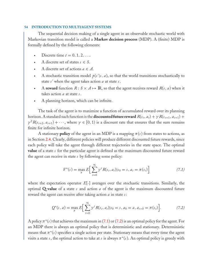
book MOBK077-Vlassis August 3, 2007 7:59
54 INTRODUCTION TO MULTIAGENT SYSTEMS
The sequential decision making of a single agent in an observable stochastic world withMarkovian transition model is called a Markov decision process (MDP). A (finite) MDP isformally defined by the following elements:
� Discrete time t = 0, 1, 2, . . ..� A discrete set of states s ∈ S.� A discrete set of actions a ∈ A.� A stochastic transition model p(s ′|s , a), so that the world transitions stochastically to
state s ′ when the agent takes action a at state s .� A reward function R : S × A �→ IR, so that the agent receives reward R(s , a) when it
takes action a at state s .� A planning horizon, which can be infinite.
The task of the agent is to maximize a function of accumulated reward over its planninghorizon. A standard such function is the discounted future reward R(s t, at) + γ R(s t+1, at+1) +γ 2 R(s t+2, at+1) + · · · , where γ ∈ [0, 1) is a discount rate that ensures that the sum remainsfinite for infinite horizon.
A stationary policy of the agent in an MDP is a mapping π (s ) from states to actions, asin Section 2.4. Clearly, different policies will produce different discounted future rewards, sinceeach policy will take the agent through different trajectories in the state space. The optimalvalue of a state s for the particular agent is defined as the maximum discounted future rewardthe agent can receive in state s by following some policy:
V ∗(s ) = maxπ
E[ ∞∑
t=0
γ t R(s t, at)|s0 = s , at = π (s t)]
(7.1)
where the expectation operator E[·] averages over the stochastic transitions. Similarly, theoptimal Q-value of a state s and action a of the agent is the maximum discounted futurereward the agent can receive after taking action a in state s :
Q∗(s , a) = maxπ
E[ ∞∑
t=0
γ t R(s t, at)|s0 = s , a0 = a, at>0 = π (s t)]. (7.2)
A policy π∗(s ) that achieves the maximum in (7.1) or (7.2) is an optimal policy for the agent. Foran MDP there is always an optimal policy that is deterministic and stationary. Deterministicmeans that π∗(s ) specifies a single action per state. Stationary means that every time the agentvisits a state s , the optimal action to take at s is always π∗(s ). An optimal policy is greedy with

book MOBK077-Vlassis August 3, 2007 7:59
LEARNING 55
respect to V ∗ or Q∗, as we have seen in Section 2.4:
π∗(s ) ∈ arg maxa
Q∗(s , a). (7.3)
Note that there can be many optimal policies in a given task, but they all share a unique V ∗
and Q∗.The definition of V ∗ in (7.1) can be rewritten recursively by making use of the transition
model, to get the so-called Bellman equation:
V ∗(s ) = maxa
[R(s , a) + γ
∑
s ′p(s ′|s , a)V ∗(s ′)
]. (7.4)
This is a set of nonlinear equations, one for each state, the solution of which defines the optimalV ∗. A similar recursive definition holds for Q-values:
Q∗(s , a) = R(s , a) + γ∑
s ′p(s ′|s , a) max
a ′Q∗(s ′, a ′). (7.5)
7.2.1 Value IterationA simple and efficient method for computing optimal values in an MDP when the transitionmodel is available is value iteration. In this method we initialize arbitrarily a Q-function (say,with all entries zero), and then we iteratively apply the Bellman equation (7.5) turned into anassignment operation:
V (s ) := maxa
Q(s , a), ∀s , (7.6)
Q(s , a) := R(s , a) + γ∑
s ′p(s ′|s , a)V (s ′), ∀s , ∀a . (7.7)
We repeat the above two equations until V does not change significantly between two con-secutive steps. Value iteration converges to the optimal Q∗ (and thus to V ∗ and π∗) for anyinitialization (Bertsekas, 2001). After we have computed Q∗ we can extract an optimal policyπ∗ using (7.3). As an example, using value iteration in the world of Fig. 2.1 of Chapter 2,with fixed reward R(s , a) = −1/30 for each nonterminal state s and action a , and with nodiscounting, we get the optimal values (utilities) and the optimal policy shown in Fig. 2.2. Thereader is encouraged to verify this by implementing the method.
7.2.2 Q-learningIn order to apply the value iteration updates (7.6) and (7.7) we need to know the transition modelp(s ′|s , a), but in many applications the transition model is unavailable. Q-learning is a methodfor estimating the optimal Q∗ (and from that an optimal policy) that does not require knowledgeof the transition model. In Q-learning the agent repeatedly interacts with the environment and
book MOBK077-Vlassis August 3, 2007 7:59
56 INTRODUCTION TO MULTIAGENT SYSTEMS
tries to estimate Q∗ by trial-and-error. As in value iteration, the agent initializes a functionQ(s , a) for each state–action pair, and then it begins exploring the environment. The explorationgenerates tuples (s , a, r, s ′) where s is a state, a is an action taken at state s , r = R(s , a) is areceived reward, and s ′ is a resulting state after executing a . From each such tuple the agentupdates its Q-value estimates as
V (s ′) := maxa ′
Q(s ′, a ′) (7.8)
Q(s , a) := (1 − λ)Q(s , a) + λ[r + γ V (s ′)
](7.9)
where λ ∈ (0, 1) is a learning rate that regulates convergence.If all state–action pairs are visited infinitely often and λ decreases slowly with time,
Q-learning converges to the optimal Q∗ (Watkins and Dayan, 1992). Moreover, this holdsirrespectively of the particular exploration policy of the agent. A common exploration policyis the so-called ε-greedy policy by which in state s the agent selects a random action withprobability ε, and action a = arg maxa ′ Q(s , a ′) with probability 1 − ε, where ε < 1 is a smallnumber. Alternatively, the agent can choose exploration action a in state s according to aBoltzmann distribution
p(a |s ) = exp(Q(s , a)/τ )∑
a ′ exp(Q(s , a ′)/τ )(7.10)
where τ controls the smoothness of the distribution (and thus the randomness of the choice),and is decreasing with time.
7.3 MARKOV GAMESIn this section we will describe a model for the simultaneous sequential decision making ofmultiple agents, and describe how reinforcement learning techniques can be extended to coverthe case of concurrently learning agents. We will throughout assume that every agent fullyobserves the current state, as in Chapter 4.
A Markov game, also known as stochastic game, can be regarded as the multiagentextension of a Markov decision process. It can also be viewed as a collection of coupled strategicgames, one per state. Formally, a Markov game is defined by the following primitives:
� Discrete time t = 0, 1, 2, . . ..� A set of n > 1 agents.� A discrete set of states s ∈ S.� For each agent i , a discrete set of actions ai ∈ Ai .� A stochastic transition model p(s ′|s , a) that is conditioned on the joint action a = (ai )
at state s .
book MOBK077-Vlassis August 3, 2007 7:59
LEARNING 57
� For each agent i , a reward function Ri : S × A �→ IR, that gives agent i reward Ri (s , a)when joint action a is taken at state s .
� A planning horizon, which can be infinite.
Note that the individual reward functions Ri (s , a) define a set of strategic games, one foreach state s . A Markov game differs to an MDP in that a transition depends on the joint actionof the agents, and that each agent may receive different reward as a result of a joint action. Asin MDPs, a policy of an agent i is a mapping πi (s ) from states to individual actions. As instrategic games, a joint policy π∗ = (π∗
i ) is a Nash equilibrium if no agent has an incentive tounilaterally change its policy; that is, no agent i would like to take at state s an action ai �= π∗
i (s )assuming that all other agents stick with their equilibrium policies π∗
−i (s ). Contrary to MDPs,in a Markov game an optimal policy of an agent need not be deterministic; we can see thisby noticing that a single-state Markov game is just a strategic game, for which we know thatdeterministic equilibria may not always exist (see Fig. 3.2(a)).
7.3.1 Independent LearningLearning in a Markov game can be done by each agent separately, ignoring the presence ofthe other agents in the system. That is, each agent can treat the other agents as part of itsenvironment, without trying to model them or predict their actions. For instance, an agent canuse Q-learning to learn its policy, as in standard MDPs, hoping that the resulting policy willperform well. However this approach is inherently flawed: the convergence of Q-learning relieson an underlying transition model that is stationary (does not change with time). This maynot be the case with concurrently learning agents, because the (hypothetical) transition modelp(s ′|s , ai ) of agent i may be changing continuously by the policy of the other agents who arealso learning.
Although independent Q-learning cannot be justified theoretically, the method hasbeen employed in practice with reported success (Mataric, 1994, Sen et al., 1994, Tan, 1993).Claus and Boutilier (1998) examine the conditions under which independent Q-learning leadsto individual policies that form a Nash equilibrium in a single state coordination problem, ar-guing that under general conditions the method converges. However, the resulting equilibriummay not be Pareto optimal. Similarly, Wolpert et al. (1999) show that for a constrained classof problems independent Q-learning may converge to a Nash equilibrium.
7.3.2 Coupled LearningBetter results can be obtained if the agents attempt to model each other, in which case theirlearning algorithms are coupled. A standard approach is to have each agent i maintain anindividual value function Vi (s ) and an individual Q-function Qi (s , a), where the latter is

book MOBK077-Vlassis August 3, 2007 7:59
58 INTRODUCTION TO MULTIAGENT SYSTEMS
defined over joint actions a . In this case, standard value iteration generalizes to Markov gamesas follows:
Vi (s ) := C(Q1(s , a), . . . , Qn(s , a)), ∀s (7.11)
Qi (s , a) := Ri (s , a) + γ∑
s ′p(s ′|s , a)Vi (s ′), ∀s , ∀a (7.12)
where C is a function that applies some solution concept to the strategic game formed by theQ1, . . . , Qn. When the transition model is not available, a corresponding coupled Q-learningupdate scheme can be derived in which (7.12) is replaced by (7.9), one per agent. Note thatsuch a multiagent Q-learning scheme requires that each agent observes the selected joint actionin each step.
Depending on the type of game (zero-sum, general-sum, or coordination game),the function C may compute a Nash equilibrium (Hu and Wellman, 2004, Littman, 1994,2001), a correlated equilibrium1 (Greenwald and Hall, 2003), or a coordinated joint ac-tion (Kok and Vlassis, 2006). Although successful in practice, the method may not alwaysbe able to compute an optimal equilibrium policy (Zinkevich et al., 2006).
7.3.3 Sparse Cooperative Q-learningHere we address the special case of collaborative agents. When all agents in a team sharethe same reward function, that is, Ri (s , a) = R(s , a) for each i , the multiagent system canbe transformed into one ‘big’ agent and solved with standard MDP techniques (Lauer andRiedmiller, 2000, Brafman and Tennenholtz, 2003). However, such an approach does not scalevery well when the number of agents is large, since the joint action space scales exponentiallyin the number of agents.
A more general case involves collaborative agents with different individual reward func-tions. A collaborative multiagent Markov decision process (CM-MDP) (Guestrin, 2003) isa Markov game model where each agent cares about maximizing the discounted future globalreward, where the latter is defined as
R(s , a) =n∑
i=1
Ri (s , a). (7.13)
Such a model allows for a decentralized learning algorithm where all update steps are local, andintermediate results are communicated by solving a global coordination game. In particular,following the general multiagent learning approach of Section 7.3.2, we can derive a multiagent
1A correlated equilibrium is a generalization of a mixed-strategy Nash equilibrium where the mixed strategies of theagents can be correlated.
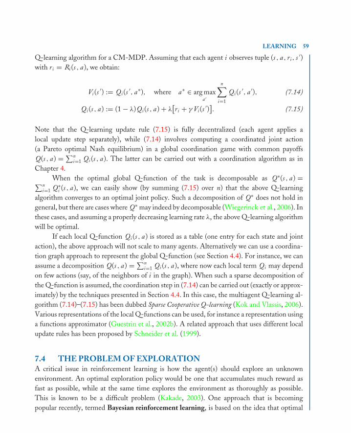
book MOBK077-Vlassis August 3, 2007 7:59
LEARNING 59
Q-learning algorithm for a CM-MDP. Assuming that each agent i observes tuple (s , a, ri , s ′)with ri = Ri (s , a), we obtain:
Vi (s ′) := Qi (s ′, a∗), where a∗ ∈ arg maxa ′
n∑
i=1
Qi (s ′, a ′), (7.14)
Qi (s , a) := (1 − λ)Qi (s , a) + λ[ri + γ Vi (s ′)
]. (7.15)
Note that the Q-learning update rule (7.15) is fully decentralized (each agent applies alocal update step separately), while (7.14) involves computing a coordinated joint action(a Pareto optimal Nash equilibrium) in a global coordination game with common payoffsQ(s , a) = ∑n
i=1 Qi (s , a). The latter can be carried out with a coordination algorithm as inChapter 4.
When the optimal global Q-function of the task is decomposable as Q∗(s , a) =∑n
i=1 Q∗i (s , a), we can easily show (by summing (7.15) over n) that the above Q-learning
algorithm converges to an optimal joint policy. Such a decomposition of Q∗ does not hold ingeneral, but there are cases where Q∗ may indeed by decomposable (Wiegerinck et al., 2006). Inthese cases, and assuming a properly decreasing learning rate λ, the above Q-learning algorithmwill be optimal.
If each local Q-function Qi (s , a) is stored as a table (one entry for each state and jointaction), the above approach will not scale to many agents. Alternatively we can use a coordina-tion graph approach to represent the global Q-function (see Section 4.4). For instance, we canassume a decomposition Q(s , a) = ∑n
i=1 Qi (s , a), where now each local term Qi may dependon few actions (say, of the neighbors of i in the graph). When such a sparse decomposition ofthe Q-function is assumed, the coordination step in (7.14) can be carried out (exactly or approx-imately) by the techniques presented in Section 4.4. In this case, the multiagent Q-learning al-gorithm (7.14)–(7.15) has been dubbed Sparse Cooperative Q-learning (Kok and Vlassis, 2006).Various representations of the local Q-functions can be used, for instance a representation usinga functions approximator (Guestrin et al., 2002b). A related approach that uses different localupdate rules has been proposed by Schneider et al. (1999).
7.4 THE PROBLEM OF EXPLORATIONA critical issue in reinforcement learning is how the agent(s) should explore an unknownenvironment. An optimal exploration policy would be one that accumulates much reward asfast as possible, while at the same time explores the environment as thoroughly as possible.This is known to be a difficult problem (Kakade, 2003). One approach that is becomingpopular recently, termed Bayesian reinforcement learning, is based on the idea that optimal

book MOBK077-Vlassis August 3, 2007 7:59
60 INTRODUCTION TO MULTIAGENT SYSTEMS
exploration can be cast as optimal planning in the space of beliefs over the unknown modelparameters, assuming a prior belief over those parameters. Planning in such a space is howeverintractable, and except for the simplest cases, approximations are needed. Poupart et al. (2006)derive the optimal exploration policy for the standard case of discrete MDPs, but the approachmay not scale in large problems (we refer to that paper for more details and references).Chalkiadakis and Boutilier (2003) describe a Bayesian reinforcement learning approach in aproblem involving a team of collaborative agents.
In a multiagent system, if we abandon the idea of collecting reward fast, and only careabout asymptotic guarantees (like convergence of Q-learning in the limit), we can often simulatein the multiagent system the conditions that ensure asymptotic convergence of single-agentlearning algorithms. For instance, in Sparse Cooperative Q-learning, the team can choose ajoint action at state s by sampling from a Boltzmann distribution over joint actions using thecurrent Q(s , a). When communication is not available, this can be achieved by having all agentsuse the same random number generator (and same seed).
Alternatively, the following exploration strategy can be used. At time t and state s ,agent i chooses at random k joint actions from the last m (m > k) observed joint actions{at−m, . . . , at−1} taken by the agents in state s . Then each agent i computes the relativefrequency of each a−i , that is, how many times out of k each a−i was taken by the other agentsat state s . This results in an empirical distribution µi (s , a−i ) that reflects the belief of agent iover the joint action a−i of all other agents at state s . Using such an empirical belief, agent ican now compute an expected payoff ui (s , ai ) for action ai at state s as
ui (s , ai ) =∑
a−i
µi (s , a−i )Q(s , [ai , a−i ]) (7.16)
and then randomly choose a best-response action a∗i ∈ arg maxai ui (s , ai ).
Variations of this approach have been used by Peyton Young (1993), Claus and Boutilier(1998), and Wang and Sandholm (2003). The approach bears resemblance to fictitious play,a learning method in games in which a number of agents interact repeatedly with each other,aiming at reaching an equilibrium (Fudenberg and Levine, 1998).
7.5 NOTES AND FURTHER READINGSingle-agent reinforcement learning is treated in the books of Bertsekas and Tsitsiklis(1996) and Sutton and Barto (1998). Fudenberg and Levine (1998), Young (2004), andGreenwald (2007) cover the subject of (reinforcement) learning in games. In the last cou-ple of years several multiagent learning algorithms have appeared in the literature. Be-sides the works cited in this chapter, notable recent works include those by Bagnell and Ng(2006), Bowling (2005), Brafman and Tennenholtz (2004), Conitzer and Sandholm (2003),

book MOBK077-Vlassis August 3, 2007 7:59
LEARNING 61
Lagoudakis and Parr (2003), Moallemi and Van Roy (2004), Peshkin et al. (2000), Singh et al.(2000), Tesauro (2004), Zinkevich et al. (2006). Multiagent reinforcement learning is still ayoung field; Shoham et al. (2007) and Gordon (2007) identify several research agendas thatcan be used for guiding research and evaluating progress.

book MOBK077-Vlassis August 3, 2007 7:59
62

book MOBK077-Vlassis August 3, 2007 7:59
63
BibliographyAdamatzky, A. and Komosinski, M., editors (2005). Artificial Life Models in Software. Springer-
Verlag, Berlin.Arnborg, S., Corneil, D. G., and Proskurowski, A. (1987). Complexity of finding embeddings
in a k-tree. SIAM Journal on Algebraic and Discrete Methods, 8(2):277–284.Aumann, R. J. (1976). Agreeing to disagree. Annals. of Statistics, 4(6):1236–1239.Bagnell, J. A. and Ng, A. Y. (2006). On local rewards and the scalability of dis-
tributed reinforcement learning. In Weiss, Y., Scholkopf, B., and Platt, J., edi-tors, Advances in Neural Information Processing Systems 18. MIT Press, Cambridge,MA.
Bellman, R. (1961). Adaptive Control Processes: a Guided Tour. Princeton University Press.Bernstein, D. S., Givan, R., Immerman, N., and Zilberstein, S. (2002). The complexity of
decentralized control of Markov decision processes. Mathematics of Operations Research,27(4):819–840. doi:10.1287/moor.27.4.819.297
Bertsekas, D. P. (2001). Dynamic Programming and Optimal Control, volume I and II. AthenaScientific, 2nd edition.
Bertsekas, D. P. and Tsitsiklis, J. N. (1996). Neuro-dynamic Programming. Athena Scientific.Bordini, R., Dastani, M., Dix, J., and El Fallah Seghrouchni, A., editors (2005). Multi-Agent
Programming: Languages, Platforms and Applications. Springer, Berlin.Boutilier, C. (1996). Planning, learning and coordination in multiagent decision pro-
cesses. In Proc. Conf. on Theoretical Aspects of Rationality and Knowledge, Renesse, TheNetherlands.
Bowling, M. (2005). Convergence and no-regret in multiagent learning. In Saul, L. K.,Weiss, Y., and Bottou, L., editors, Advances in Neural Information Processing Systems 17,pp. 209–216. MIT Press, Cambridge, MA.
Brafman, R. I. and Tennenholtz, M. (2003). Learning to coordinate efficiently: A model basedapproach. Journal of Artificial Intelligence Research, 19:11–23.
Brafman, R. I. and Tennenholtz, M. (2004). Efficient learning equilibrium. Artificial Intelli-gence, 159(1-2):27–47. doi:10.1016/j.artint.2004.04.013
Castelpietra, C., Iocchi, L., Nardi, D., Piaggio, M., Scalzo, A., and Sgorbissa, A. (2000).Coordination among heterogenous robotic soccer players. In Proc. IEEE/RSJ Int. Conf. onIntelligent Robots and Systems, Takamatsu, Japan.

book MOBK077-Vlassis August 3, 2007 7:59
64 INTRODUCTION TO MULTIAGENT SYSTEMS
Chalkiadakis, G. and Boutilier, C. (2003). Coordination in multiagent reinforcement learning:A Bayesian approach. In Proc. 2nd Int. Joint Conf. on Autonomous Agents and MultiagentSystems, Melbourne, Australia.
Clarke, E. H. (1971). Multipart pricing of public goods. Public Choice, 11:17–33.doi:10.1007/BF01726210
Claus, C. and Boutilier, C. (1998). The dynamics of reinforcement learning in cooperativemultiagent systems. In Proc. 15th Nation. Conf. on Artificial Intelligence, Madison, WI.
Cohen, P. R. and Levesque, H. J. (1991). Teamwork. Nous, 25(4):487–512.Conitzer, V. (2006). Computational Aspects of Preference Aggregation. PhD thesis, Computer
Science Department, Carnegie Mellon University.Conitzer, V. and Sandholm, T. (2003). AWESOME: A general multiagent learning algorithm
that converges in self-play and learns a best response against stationary opponents. In Proc.20th Int. Conf. on Machine Learning, Washington, DC, USA.
Conitzer, V. and Sandholm, T. (2007). Incremental mechanism design. In Proc. 20th Int. JointConf. on Artificial Intelligence, Hyderabad, India.
Conte, R. and Dellarocas, C., editors (2001). Social Order in Multiagent Systems. Kluwer Aca-demic, Dordrecht.
Cramton, P., Shoham, Y., and Steinberg, R., editors (2006). Combinatorial Auctions. MITPress, Cambridge, MA.
Dechter, R. (2003). Constraint Processing. Morgan Kaufmann, San Mates, CA.Decker, K. and Lesser, V. R. (1995). Designing a family of coordination algorithms. In Proc.
1st Int. Conf. on Multi-Agent Systems, San Francisco, CA.Durfee, E. H. and Lesser, V. R. (1987). Using partial global plans to coordinate dis-
tributed problem solvers. In Proc. 10th Int. Joint Conf. on Artificial Intelligence, Milan,Italy.
Emery-Montemerlo, R., Gordon, G., Schneider, J., and Thrun, S. (2005). Game theoreticcontrol for robot teams. In Proc. IEEE Int. Conf. on Robotics and Automation, Barcelona,Spain.
Fagin, R., Halpern, J., Moses, Y., and Vardi, M. (1995). Reasoning about Knowledge. The MITPress, Cambridge, MA.
Ferber, J. (1999). Multi-Agent Systems: An Introduction to Distributed Artificial Intelligence.Addison-Wesley, Reading, MA.
Fudenberg, D. and Levine, D. K. (1998). The Theory of Learning in Games. MIT Press,Cambridge, MA.
Geanakoplos, J. (1992). Common knowledge. Journal of Economic Perspectives, 6(4):53–82.Gibbard, A. (1973). Manipulation of voting schemes: a general result. Econometrica, 41:587–
601. doi:10.2307/1914083
book MOBK077-Vlassis August 3, 2007 7:59
BIBLIOGRAPHY 65
Gibbons, R. (1992). Game Theory for Applied Economists. Princeton University Press, Princeton,NJ.
Gilbert, N. and Doran, J., editors (1994). Simulating Societies: The Computer Simulation of SocialPhenomena. UCL Press, London.
Gmytrasiewicz, P. J. and Durfee, E. H. (2001). Rational communication inmulti-agent environments. Autonomous Agents and Multi-Agent Systems, 4:233–272.doi:10.1023/A:1011495811107
Gordon, G. J. (2007). Agendas for multi-agent learning. Artificial Intelligence. doi:10.1016/j.artint.2006.12.006.
Greenwald, A. (2007). The Search for Equilibrium in Markov Games (Synthesis Lectures onArtificial Intelligence and Machine Learning). Morgan & Claypool Publishers, San Rafael,CA.
Greenwald, A. and Hall, K. (2003). Correlated-Q learning. In Proc. 20th Int. Conf. on MachineLearning, Washington, DC, USA.
Groves, T. (1973). Incentives in teams. Econometrica, 41:617–631. doi:10.2307/1914085Guestrin, C. (2003). Planning Under Uncertainty in Complex Structured Environments. PhD
thesis, Computer Science Department, Stanford University.Guestrin, C., Koller, D., and Parr, R. (2002a). Multiagent planning with factored MDPs. In
Dietterich, T. G., Becker, S., and Ghahramani, Z., editors, Advances in Neural InformationProcessing Systems 14. The MIT Press, Cambridge, MA.
Guestrin, C., Lagoudakis, M., and Parr, R. (2002b). Coordinated reinforcement learning. InProc. 19th Int. Conf. on Machine Learning, Sydney, Australia.
Hansen, E. A., Bernstein, D. S., and Zilberstein, S. (2004). Dynamic programming for partiallyobservable stochastic games. In Proc. 19th National Conf. on Artificial Intelligence, San Jose,CA.
Harsanyi, J. C. (1967). Games with incomplete information played by ‘Bayesian’ players, PartsI, II, and III. Management Science, 14:159–182, 320–334, and 486–502.
Harsanyi, J. C. and Selten, R. (1988). A General Theory of Equilibrium Selection in Games, MITPress, Cambridge, MA.
Hu, J. and Wellman, M. P. (2004). Nash Q-learning for general-sum stochastic games. Journalof Machine Learning Research, 4:1039–1069. doi:10.1162/1532443041827880
Huhns, M. N., editor (1987). Distributed Artificial Intelligence. Pitman, Morgan Kaufmann,San Mateo, CA.
Jennings, N. R. (1996). Coordination techniques for distributed artificial intelligence. InO’Hare, G. M. P. and Jennings, N. R., editors, Foundations of Distributed Artificial In-telligence, pp. 187–210. John Wiley & Sons, New York.
Kakade, S. (2003). On the Sample Complexity of Reinforcement Learning. PhD thesis, GatsbyComputational Neuroscience Unit, University College London.
book MOBK077-Vlassis August 3, 2007 7:59
66 INTRODUCTION TO MULTIAGENT SYSTEMS
Kitano, H., Tambe, M., Stone, P., Veloso, M., Coradeschi, S., Osawa, E., Matsubara, H.,Noda, I., and Asada, M. (1997). The RoboCup synthetic agent challenge 97. In Proc. Int.Joint Conf. on Artificial Intelligence, Nagoya, Japan.
Kok, J. R., Spaan, M. T. J., and Vlassis, N. (2005). Non-communicative multi-robot co-ordination in dynamic environments. Robotics and Autonomous Systems, 50(2–3):99–114.doi:10.1016/j.robot.2004.08.003
Kok, J. R. and Vlassis, N. (2006). Collaborative multiagent reinforcement learning by payoffpropagation. Journal of Machine Learning Research, 7:1789–1828.
Kowalczyk, W. and Vlassis, N. (2005). Newscast EM. In Saul, L. K., Weiss, Y., and Bottou,L., editors, Advances in Neural Information Processing Systems 17, pp. 713–720. MIT Press,Cambridge, MA.
Lagoudakis, M. G. and Parr, R. (2003). Learning in zero-sum team Markov games usingfactored value functions. In Becker, S., Thrun, S., and Obermayer, K., editors, Advances inNeural Information Processing Systems 15, MIT Press, Cambridge, MA.
Lauer, M. and Riedmiller, M. (2000). An algorithm for distributed reinforcement learning incooperative multi-agent systems. In Proc. 17th Int. Conf. on Machine Learning, StanfordUniversity, USA.
Lesser, V., Ortiz Jr., C. L., and Tambe, M., editors (2003). Distributed Sensor Networks: AMultiagent Perspective. Kluwer Academic, Dodrecht.
Lewis, D. K. (1969). Conventions: A Philosophical Study. Harvard University Press, Cambridge.Littman, M. L. (1994). Markov games as a framework for multi-agent reinforcement learning.
In Proc. 11th Int. Conf. on Machine Learning, San Francisco, CA.Littman, M. L. (2001). Friend-or-foe Q-learning in general-sum games. In Proc. 18th Int.
Conf. on Machine Learning, San Francisco, CA.Mataric, M. J. (1994). Reward functions for accelerated learning. In Proc. 11th Int. Conf. on
Machine Learning, San Francisco, CA.Moallemi, C. C. and Van Roy, B. (2004). Distributed optimization in adaptive networks. In
Thrun, S., Saul, L., and Scholkopf, B., editors, Advances in Neural Information ProcessingSystems 16. MIT Press, Cambridge, MA.
Modi, P. J., Shen, W.-M., Tambe, M., and Yokoo, M. (2005). ADOPT: Asynchronousdistributed constraint optimization with quality guarantees. Artificial Intelligence, 161(1–2):149–180. doi:10.1016/j.artint.2004.09.003
Nash, J. F. (1950). Equilibrium points in n-person games. Proceedings of the National Academyof Sciences, 36:48–49. doi:10.1073/pnas.36.1.48
Nisan, N. (1999). Algorithms for selfish agents. In Proc. 16th Symp. on Theoret. Aspects ofComputer Science, Trier, Germany.
book MOBK077-Vlassis August 3, 2007 7:59
BIBLIOGRAPHY 67
Nisan, N., Tardos, E., and Vazirani, V., editors (2007). Algorithmic Game Theory. CambridgeUniversity Press, Cambridge.
Noriega, P. and Sierra, C., editors (1999). Agent Mediated Electronic Commerce. Lecture Notesin Artificial Intelligence 1571. Springer, Berlin.
O’Hare, G. M. P. and Jennings, N. R., editors (1996). Foundations of Distributed ArtificialIntelligence. John Wiley & Sons, New York.
Oliehoek, F. A. and Vlassis, N. (2007). Q-value functions for decentralized POMDPs. In Proc.of Int. Joint Conf. on Autonomous Agents and Multi Agent Systems, Honolulu, Hawai’i.
Osborne, M. J. (2003). An Introduction to Game Theory. Oxford University Press, Oxford.Osborne, M. J. and Rubinstein, A. (1994). A Course in Game Theory. MIT Press, Cambridge,
MA.Papadimitriou, C. H. (2001). Algorithms, games, and the Internet. In Proc. 33rd Ann. ACM
Symp. on Theory of Computing, Heraklion, Greece.Papadimitriou, C. H. and Tsitsiklis, J. N. (1987). The complexity of Markov decision processes.
Mathematics of Operations Research, 12(3):441–450.Parkes, D. C. (2001). Iterative Combinatorial Auctions: Achieving Economic and Computational
Efficiency. PhD thesis, Computer and Information Science, University of Pennsylvania.Parkes, D. C. and Shneidman, J. (2004). Distributed implementations of Vickrey-Clarke-
Groves mechanisms. In Proc. 3nd Int. Joint Conf. on Autonomous Agents and MultiagentSystems, New York, USA.
Paskin, M. A., Guestrin, C. E., and McFadden, J. (2005). A robust architecture for distributedinference in sensor networks. In Proc. 4th Int. Symp. on Information Processing in SensorNetworks, Los Angeles, CA.
Pearce, J. P. and Tambe, M. (2007). Quality guarantees on k-optimal solutions for distributedconstraint optimization problems. In Proc. 20th Int. Joint Conf. on Artificial Intelligence,Hyderabad, India.
Pearl, J. (1988). Probabilistic Reasoning in Intelligent Systems. Morgan Kaufman, San Mateo,CA.
Peshkin, L., Kee-Eung, K., Meuleau, N., and Kaelbling, L. (2000). Learning to cooperate viapolicy search. In Proc. 16th Int. Conf. on Uncertainty in Artificial Intelligence, San Francisco,CA.
Peyton Young, H. (1993). The evolution of conventions. Econometrica, 61(1):57–84.doi:10.2307/2951778
Porter, R., Nudelman, E., and Shoham, Y. (2004). Simple search methods for finding a Nashequilibrium. In Proc. 19th National Conf. on Artificial Intelligence, San Jose, CA.
Poupart, P., Vlassis, N., Hoey, J., and Regan, K. (2006). An analytic solution to discreteBayesian reinforcement learning. In Proc. Int. Conf. on Machine Learning, Pittsburgh, USA.
book MOBK077-Vlassis August 3, 2007 7:59
68 INTRODUCTION TO MULTIAGENT SYSTEMS
Roumeliotis, S. I. and Bekey, G. A. (2002). Distributed multi-robot localization. IEEE Trans.Robotics and Automation, 18(5):781–795. doi:10.1109/TRA.2002.803461
Russell, S. J. and Norvig, P. (2003). Artificial Intelligence: a Modern Approach. Prentice Hall,Englewood Cliffs, NJ, 2nd edition.
Samet, D. (2006). Agreeing to disagree: the non-probabilistic case. Unpublished manuscript(available from http://www.tau.ac.il/˜samet).
Sandell, N. R., Varayia, P., Athans, M., and Safonov, M. G. (1978). Survey of decentralizedcontrol methods for large-scale systems. IEEE Trans. Automatic Control, AC-23(2):108–128. doi:10.1109/TAC.1978.1101704
Sandholm, T. (1999). Distributed rational decision making. In Weiss, G., editor, MultiagentSystems: A Modern Introduction to Distributed Artificial Intelligence, pp. 201–258. MIT Press,Cambridge, MA.
Schneider, J., Wong, W.-K., Moore, A., and Riedmiller, M. (1999). Distributed value func-tions. In Proc. Int. Conf. on Machine Learning, Bled, Slovenia.
Sen, S., Sekaran, M., and Hale, J. (1994). Learning to coordinate without sharing information.In Proc. 12th Nation. Conf. on Artificial Intelligence, Seattle, WA.
Shoham, Y. and Leyton-Brown, K. (2007). Multi-Agent Systems. Cambridge University Press,Cambridge.
Shoham, Y., Powers, R., and Grenager, T. (2007). If multi-agent learning is the answer, whatis the question? Artificial Intelligence. doi: 10.1016/j.artint.2006.02.006.
Shoham, Y. and Tennenholtz, M. (1992). On the synthesis of useful social laws for ar-tificial agent societies. In Proc. 10th Nation. Conf. on Artificial Intelligence, San Diego,CA.
Singh, M. P. (1994). Multiagent Systems: A Theoretical Framework for Intentions, Know-How,and Communications. Springer-Verlag, Berlin.
Singh, S., Kearns, M., and Mansour, Y. (2000). Nash convergence of gradient dynamics ingeneral-sum games. In Proc. 16th Int. Conf. on Uncertainty in Artificial Intelligence, SanFrancisco, CA.
Smith, R. G. (1980). The contract net protocol: high-level communication and control in adistributed problem solver. IEEE Trans. Computers, C-29(12):1104–1113.
Spaan, M. T. J. and Vlassis, N. (2005). Perseus: Randomized point-based value iteration forPOMDPs. Journal of Artificial Intelligence Research, 24:195–220.
Stone, P. (2000). Layered Learning in Multiagent Systems: A Winning Approach to Robotic Soccer.MIT Press, Cambridge, MA.
Stone, P. and Veloso, M. (2000). Multiagent systems: a survey from a machine learningperspective. Autonomous Robots, 8(3).

book MOBK077-Vlassis August 3, 2007 7:59
BIBLIOGRAPHY 69
Sutton, R. S. and Barto, A. G. (1998). Reinforcement Learning: An Introduction. MIT Press,Cambridge, MA.
Sycara, K. (1998). Multiagent systems. AI Magazine, 19(2):79–92.Symeonidis, A. L. and Mitkas, P. A., editors (2006). Agent Intelligence Through Data Mining.
Springer, Berlin.Tan, M. (1993). Multi-agent reinforcement learning: Independent vs. cooperative agents. In
Proc. 10th Int. Conf. on Machine Learning, Amherst, MA.Terzopoulos, D. (1999). Artificial life for computer graphics. Commun. ACM, 42(8):32–42.
doi:10.1145/310930.310966Tesauro, G. (2004). Extending Q-learning to general adaptive multi-agent systems. In Thrun,
S., Saul, L., and Scholkopf, B., editors, Advances in Neural Information Processing Systems16. MIT Press, Cambridge, MA.
Thorndike, E. L. (1898). Animal Intelligence: An Experimental Study of the Associative Processesin Animals. PhD thesis, Columbia University.
Vickrey, W. (1961). Counterspeculation, auctions, and competitive sealed tenders. Journal ofFinance, 16:8–37. doi:10.2307/2977633
Vidal, J. M. (2007). Fundamentals of Multiagent Systems with NetLogo Examples. Electronicallyavailable at www.multiagent.com.
Vlassis, N., Elhorst, R. K., and Kok, J. R. (2004). Anytime algorithms for multiagent decisionmaking using coordination graphs. In Proc. Int. Conf. on Systems, Man and Cybernetics, TheHague, The Netherlands.
von Neumann, J. and Morgenstern, O. (1944). Theory of Games and Economic Behavior. JohnWiley & Sons, New York.
von Stengel, B. (2007). Equilibrium computation for two-player games in strategic and exten-sive form. In Nisan, N., Tardos, E., and Vazirani, V., editors, Algorithmic Game Theory.Cambridge University Press, Cambridge.
Wainwright, M. J., Jaakkola, T. S., and Willsky, A. S. (2004). Tree consistency and boundson the performance of the max-product algorithm and its generalizations. Statistics andComputing, 14:143–166. doi:10.1023/B:STCO.0000021412.33763.d5
Wang, X. and Sandholm, T. (2003). Reinforcement learning to play an optimal Nash equi-librium in team Markov games. In Becker, S., Thrun, S., and Obermayer, K., editors,Advances in Neural Information Processing Systems 15, MIT Press, Cambridge, MA.
Watkins, C. J. C. H. and Dayan, P. (1992). Q-learning. Machine Learning, 8(3):279–292.Weiss, G., editor (1999). Multiagent Systems: a Modern Approach to Distributed Artificial Intel-
ligence. MIT Press, Cambridge, MA.Wiegerinck, W., van den Broek, B., and Kappen, B. (2006). Stochastic optimal control in
continuous space-time multi-agent systems. In Proc. 22th Int. Conf. on Uncertainty inArtificial Intelligence, MIT Press, Cambridge, MA.
book MOBK077-Vlassis August 3, 2007 7:59
70 INTRODUCTION TO MULTIAGENT SYSTEMS
Wolpert, D., Wheeler, K., and Tumer, K. (1999). General principles of learning-based multi-agent systems. In Proc. 3rd Int. Conf. on Autonomous Agents, Seattle, WA.
Wooldridge, M. (2002). An Introduction to MultiAgent Systems. John Wiley & Sons, New York.Xiang, Y. (2002). Probabilistic Reasoning in Multiagent Systems: A Graphical Models Approach.
Cambridge University Press, Cambridge.Yokoo, M. (2000). Distributed Constraint Satisfaction: Foundation of Cooperation in Multi-agent
Systems. Springer, Berlin.Young, H. P. (2004). Strategic learning and its limits. Oxford University Press, Oxford.Zhang, W., Wang, G., Xing, Z., and Wittenberg, L. (2005). Distributed stochas-
tic search and distributed breakout: Properties, comparison and applications to con-straint optimization problems in sensor networks. Artificial Intelligence, 161(1-2):55–87.doi:10.1016/j.artint.2004.10.004
Zinkevich, M., Greenwald, A., and Littman, M. L. (2006). Cyclic equilibria in Markov games.In Weiss, Y., Scholkopf, B., and Platt, J., editors, Advances in Neural Information ProcessingSystems 18, pp. 1641–1648. MIT Press, Cambridge, MA.
book MOBK077-Vlassis August 3, 2007 7:59
71
Author BiographyNikos Vlassis was born in 1970 in Corinth, Greece. He received an MSc (1993) and a PhD(1998) in Electrical and Computer Engineering from the National Technical University ofAthens, Greece. In 1998 he joined the Informatics Institute of the University of Amsterdam,The Netherlands, as research fellow, and in 1999 he visited the Electrotechnical Labora-tory (ETL, currently AIST) in Tsukuba, Japan, with a scholarship from the Japan IndustrialTechnology Association (MITI). From 2000 until 2006 he held an Assistant Professor posi-tion in the Informatics Institute of the University of Amsterdam, The Netherlands. Since 2007he holds an Assistant Professor position in the Department of Production Engineering andManagement of the Technical University of Crete, Greece. He is coauthor of about 100 paperson various topics in the fields of machine learning, multiagent systems, robotics, and computervision, and has received numerous citations. Awards that he has received include the DimitrisChorafas Foundation prize for young researchers in Engineering and Technology (Luzern,Switzerland, 1998), best-teacher mention at the University of Amsterdam (2001–2005), bestscientific paper award with the paper ‘Using the max-plus algorithm for multiagent decisionmaking in coordination graphs’ in the annual RoboCup symposium (2005), and various dis-tinctions with the UvA Trilearn robot soccer team including the 1st position at the RoboCupworld championship (2003). His current research interests are in the areas of robotics, machinelearning, and stochastic optimal control.

book MOBK077-Vlassis August 3, 2007 7:59
72