A consistent view on the terrestrial carbon cycle through simultaneous assimilation of multiple data streams into a model of the

terrestrial carbon cycle

RIKEN International Symposium on Data Assimilation 27 Februar – 2 March 2017, Kobe, Japan

Marko Scholze1, T. Kaminski2, W. Knorr1, Peter Rayner3 and Gregor Schürmann4

1 Lund University, Sweden 2 The Inversion Lab, Hamburg, Germany 3 University of Melbourne, Australia 4 Max Planck Institute for Biogeochemisty, Jena, Germany

Outline

• Introduction • Carbon Cycle Data Assimilation System • Multiple constraints • Non-convergence problem • Conclusions

The Global Carbon Cycle

Global Carbon Budget

1.0±0.5 PgC/yr 10%

2.6±0.8 PgC/yr

Land 28%

4.3±0.1 PgC/yr

Atmosphere 46%

2.5±0.5 PgC/yr

Oceans 26%

8.3±0.4 PgC/yr 90%

+

The case for data assimilation

⇒ Carbon Cycle Data Assimilation System = ecophysiological constraints from forward modelling + observational constraints from inverse modelling

Large uncertainty from land to predict C-balance (GCP)

C fl

ux to

land

(Pg

C/y

r)

Available Observations

Le Quéré et al. 2013

CCDAS methodology Based on process-based terrestrial ecosystem model (BETHY) Optimizing parameter values (~100) based on gradient info Hessian (2nd deriv.) to estimate posterior parameter uncertainty Error propagation by using linearised model

Scholze et al. (2007)

Process parameters

• Process parameters are invariant in time • Parameterisations in biological systems are often based

on (semi-)empirical relationships -> no universal/fundamental theory as in physical systems

• Parameters are often plant species specific but model lumps together many species into a plant functional and this upscaling process is highly uncertain

CCDAS approach

Optimizer J(X) and dJ(X)/X

Flux-tower data CO2 exchange

PFT composition ecosystem parameters initial conditions

parameters (X) ≠

J(X) M(X)

yflux

Terrestrial ecosystem

model Satellite data: veg. activity & soil moisture

ysat

J(X) J(X)

Climate

Ground-based atm CO2 yCO2

Adjoint model dJ(X)/X

Cost function:

Need to define the error matrices Cy-1, Cp

-1

BETHY

Knorr (2000)

The atm. CO2 flask station network

Mauna Loa

South Pole

Pt. Barrow

Single constraint atm. CO2: data fit

Rayner et al., 2005

Posterior uncertainties on parameters

examples:

Inverse Hessian of cost function approximates posterior uncertainties

Relative Error Reduction 1–σopt/σprior

Rayner et al., 2005

Net C fluxes and their uncertainties

Examples for diagnostics: • Long term mean fluxes to atmosphere

(gC/m2/year) and uncertainties • Regional means

Rayner et al., 2005

atm. CO2 CO2 flask +

Uncertainties

Multiple constraints, 1st example

Consistent Assimilation : • all data streams jointly • in a single long assimilation window

Transfer of information in space and between variables

Hyytiala

Improved GPP

Schuermann et al. (2016)

Loobos

Transfer of information in space

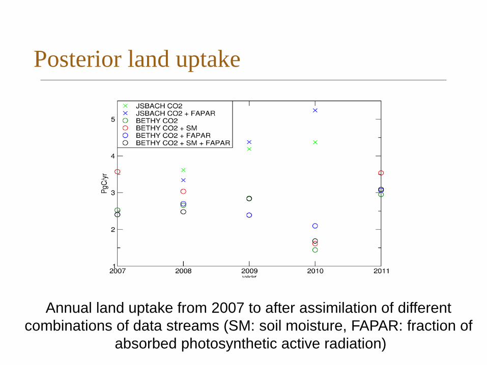
Posterior land uptake

Annual land uptake from 2007 to after assimilation of different combinations of data streams (SM: soil moisture, FAPAR: fraction of

absorbed photosynthetic active radiation)

Multiple constraints, 2nd example

• Simultaneous assimilation of two data streams at site level

Maun, Botswana over 2 years (2000-2001) • Daily LE fluxes, no gap-filled data (464 observations) • Satellite FAPAR observations, 10-daily (70 observations) • Optimization of 24 model parameters • 2 Plant Functional Types: tropical broadleaf deciduous tree

and C4 grass

Kato et al. (2012), Biogeosciences

Fit to LE and FAPAR data

Relative reduction:

(LE)

Posterior parameter uncertainty

Parameter

Robustness of optimal solution • Different starting point -> same minimum? • Local minimum vs global minimum • Non-convergence problems

Global minimum?

Find sub-set of model which converges using 4D-var, use ensemble for remaining model

-> combined ensemble-adjoint optimisation

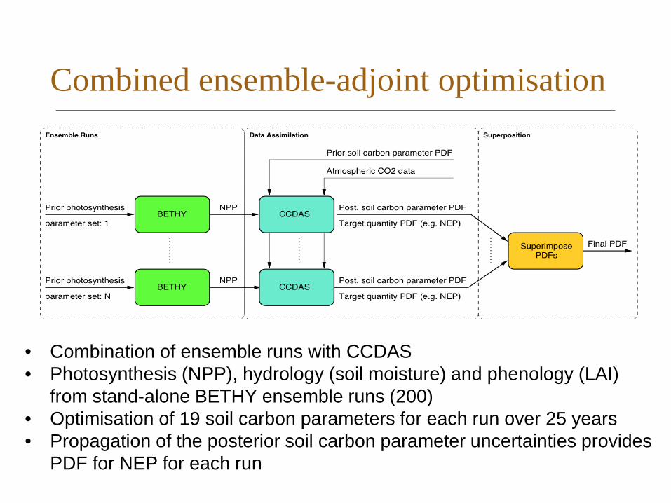
Combined ensemble-adjoint optimisation

• Combination of ensemble runs with CCDAS • Photosynthesis (NPP), hydrology (soil moisture) and phenology (LAI)

from stand-alone BETHY ensemble runs (200) • Optimisation of 19 soil carbon parameters for each run over 25 years • Propagation of the posterior soil carbon parameter uncertainties provides

PDF for NEP for each run

Results for a test case: individual cost functions

170 out of 200 member ensemble kept, 30 runs are discarded due to non-convergence or non-physical posterior parameter values.

Test case: posterior parameter unc.

Blue: Individual PDFs obtained from CCDAS using input from ensemble Red: Superimposed PDF Green: Gaussian approximation

Results for a test case: global net C flux

Blue: Individual PDFs obtained from CCDAS using input from ensemble runs Red: Superimposed PDF Green: Gaussian Approximation Black: Base case PDF

Summary • CCDAS: Mathematically rigorous combination of process

understanding and observations for carbon cycling • Provides integrated view on global carbon cycle on all variables that

can be simulated by the model at any time and place • Regional scale carbon budgets based on combination of multiple

data streams and process-based simulations • Added value of data streams quantified through uncertainty reduction • Can be extended to include further data streams, either for

assimilation or validation • Hierarchical Parameter Estimation

– Combination of ensemble runs and 4D-Var in a data assimilation system – Superimpose individual PDFs for parameters and target quantities to

obtain final PDF

Fit against GPP

-2

0

2

4

6

8

1 4 7 10 1 4 7 10 1

ObsPriorExp. 1 (LHF)Exp. 2 (FAPAR)Exp. 3 (Combined)

GPP

(gC

m-2

day

-1)