European Journal of Operational Research 220 (2012) 251–261

Contents lists available at SciVerse ScienceDirect

European Journal of Operational Research

journal homepage: www.elsevier .com/locate /e jor

Innovative Applications of O.R.

A Constraint Programming model for fast optimal stowage of container vessel bays

Alberto Delgado a,⇑, Rune Møller Jensen a, Kira Janstrup b, Trine Høyer Rose b, Kent Høj Andersen c

a IT University of Copenhagen, Rued Langgaards Vej 7, 2300 Copenhagen S, Denmarkb Copenhagen University, Universitetspark 5, 2100 Copenhagen Ø, Denmarkc Århus University, Ny Munkegade 118, 8000 Århus C, Denmark

a r t i c l e i n f o

Article history:Received 3 November 2010Accepted 15 January 2012Available online 24 January 2012

Keywords:Container vessel stowage planningSlot planningConstraint ProgrammingInteger Programming

0377-2217/$ - see front matter � 2012 Elsevier B.V. Adoi:10.1016/j.ejor.2012.01.028

⇑ Corresponding author. Tel.: +45 72185085; fax: +E-mail addresses: alde@itu.dk (A. Delgado), rmj@itu.

dtu.dk (K. Janstrup), m01thr@math.ku.dk (T.H. Rose), ke

a b s t r a c t

Container vessel stowage planning is a hard combinatorial optimization problem with both high eco-nomic and environmental impact. We have developed an approach that often is able to generate near-optimal plans for large container vessels within a few minutes. It decomposes the problem into a masterplanning phase that distributes the containers to bay sections and a slot planning phase that assigns con-tainers of each bay section to slots. In this paper, we focus on the slot planning phase of this approach andpresent a Constraint Programming and Integer Programming model for stowing a set of containers in asingle bay section. This so-called slot planning problem is NP-hard and often involves stowing severalhundred containers. Using state-of-the-art constraint solvers and modeling techniques, however, wewere able to solve 90% of 236 real instances from our industrial collaborator to optimality within 1 sec-ond. Thus, somewhat to our surprise, it is possible to solve most of these problems optimally within thetime required for practical application.

� 2012 Elsevier B.V. All rights reserved.

1. Introduction

Approximately 90% of all non-bulk cargo is carried in containervessels. An important economical parameter for liner shippingcompanies is to be able to stow their vessels fast. This not onlysaves port fees but also decreases the speed at sea which savesbunker and reduces CO2 emissions. Most stowage plans areproduced manually by stowage coordinators using graphical tools,but due to the hardness of the problem and a potential for substan-tial savings, there recently has been an increasing interest inextending these tools with stowage planning optimization algo-rithms. These algorithms must also be fast, since stowage coordi-nators work under time pressure and may have to recomputeplans due to loadlist changes or for the sake of evaluating differentforecast scenarios. A runtime of more than 10 minutes is impracti-cal according to our industrial collaborator within the liner ship-ping industry.

We have developed a stowage planning optimization approachthat similar to the currently most successful approaches (e.g.,[21,14,1]), decomposes the problem hierarchically. We use the2-phase approach illustrated in Fig. 1. First, the master planningphase distributes the containers to load in the port to bay sectionsof the vessel. The slot planning phase then assigns the containers toload in each bay section to specific slots.

ll rights reserved.

45 72185001.dk (R.M. Jensen), kj@transport.nt@imf.au.dk (K.H. Andersen).

Our master planning approach has been presented in [16]. Thefocus of this paper is the slot planning phase.1 A typical large con-tainer vessel has about 100 bay sections, which implies that the slotplanning phase solves about 100 independent slot planning prob-lems. Thus, given at most 10 minutes to generate complete stowageplans including master planning on hardware that does not supportheavy parallelization, we aim at solving each slot planning problemin less than 1 second. This is non-trivial since slot planning is NP-hard and each bay section may hold up to several hundredcontainers.

Real slot planning problems include a wide variety of vesselstructures and containers. To make their study practical, we intro-duce the Container Stowage Problem for Below Deck Locations(CSPBDL), a representative model for stowing containers in baysections below deck formulated together with our industrial col-laborator. Even though this is a simplified representation of theproblem, it is to our knowledge the most detailed model publishedto date.

We then introduce an Integer Programming (IP) and ConstraintProgramming (CP) model for solving the CSPBDL to optimality. TheCP model uses state-of-the-art modeling techniques includingmultiple viewpoints, specific domain pruning rules, and dynamiclower bounds. The IP model is a 0–1 formulation where cuts areintroduced to strengthen the LP relaxation.

1 An early version of this work has been presented at the International Conferenceon Principles and Practice of Constraint Programming in 2009 [9].

PlanningSlot

PlanningSlot Slot Plan

1

PlanningSlot

Slot Plan

Slot Plan2

n

... ... ...

Section 2Bay

Section n

Section 1Bay

Bay

StowagePlan

LoadlistsVessel DataPort Data

Master

Planning

Slot Planning PhaseMaster Planning Phase

Fig. 1. The master planning and slot planning decomposition of stowage planning.

252 A. Delgado et al. / European Journal of Operational Research 220 (2012) 251–261

Despite the size and NP-hardness of slot planning problems, ourcomputational results show that they often can be solved fast inpractice. We have derived 236 test instances from real stowageplans from a system deployed by our industrial collaborator [12].92% of the instances are solved using a state-of-the-art constraintsolver on our CP model within 1 second. Similar but slightly worseresults were obtained with the IP model. Thus, somewhat to oursurprise, it is possible to define optimal models of slot planningproblems that can be solved fast enough to be used in stowageplanning optimization tools.

The rest of the paper is organized as follows. Section 2 definesthe problem we address in this paper and related work is pre-sented and Section 3. In Section 4, we give a detailed descriptionof our IP model. Section 5 gives a brief introduction to globalconstraint modeling, and in Section 6 we present our CP model.Computational results are presented in Section 7 and conclusionsand directions for future work are discussed in Section 8.

2. Problem statement

A container vessel is a ship that transports box formed contain-ers on a fixed cyclic route. The cargo space of a vessel is dividedinto bays. Each bay is divided into an on deck and below deck partby a hatch cover, which is a flat, leak-proof structure that preventsthe vessel from taking in water and allows containers to be stowedon top of it (see Fig. 2). On and below deck parts of a bay are trans-versally divided into stacks that are one container wide, and arecomposed of two Twenty-foot Equivalent Unit (TEU) stacks and asingle Forty-foot Equivalent Unit (FEU) stack. A location is a baysection consisting of a set of stacks that are either on or belowdeck. These stacks are not necessarily adjacent. The left drawingof Fig. 3 shows a typical arrangement of locations in a bay. A stackholds vertically arranged cells indexed by tiers. Each stack has aweight and height limit that must be satisfied by the containersallocated there. Cells in stacks are divided into two slots, a foreand an aft. The aft slot is situated toward the stern of the vessel,while the fore slot is allocated on the bow side.2 Some slots havea power plug to provide electricity to containers in case their cargoneeds to be refrigerated. Such slots are called reefer slots. Quay cranesat ports carry out the loading and unloading of containers from thevessel accessing only the top-most containers in stacks.

A container is a metal box in which goods can be stored. Eachcontainer has a weight, height, length, and port where it has tobe unloaded (discharge port), and may need to be provided withelectric power (reefer container). Containers are 200, 400, or 450 long,and 80600 or 90600 high (high-cube containers). High-cube 200 foot con-tainers are rare and we assume they do not exist when modelingthe slot planning problem. Empty 200 and 400 containers weightaround two tons while their maximum weight is 24 and 30 tons,

2 The liner shipping industry uses another indexing standard for bays, stacks andtiers than the one presented in this paper which is irrelevant for our purposes.

respectively. Pallet wide containers are slightly wider and can onlybe placed side-by-side in certain patterns. IMO containers carrydangerous goods and must be placed according to a complex setof separation rules. Out-of-Gauge containers carry cargo exceedingthe inner dimensions of standard containers. The last three typesof containers are often placed in special storage areas of the vessel.

Each cell can hold one 400 or 450 container or two 200 containers.The 450 containers, however, are normally only placed on deck, andsome cells may be restricted to either 200 or 400 containers. In addi-tion, odd cells may exist that only can hold one 200 container due tothe physical layout of the vessel. As an example, the right picture ofFig. 3 shows the slots of a stack below deck with a mixture of dif-ferent 200 and 400 containers loaded. Containers already on boardof the vessel when the stowage plan is made are called loaded con-tainers. A container in a stack is overstowing another container inthe same stack if it is stowed above it and discharged at a laterport. An overstowing container is expensive, since it must be re-moved in order to discharge the overstowed container.

In this paper, we investigate the slot planning problem which isto assign a set of containers to slots in a location that may alreadyhold loaded containers. Due to the large number of constraints andobjectives involved in real slot planning, we have developed withour industrial collaborator a representative version of the problemfor below deck locations called the CSPBDL. On deck locations sharemost constraints and objectives with below deck locations, thus weexpect similar computational results for them. The CSPBDL coversall constraint and objective classes of the problem, and we antici-pate a high correlation with a complete problem model in termsof solution algorithm performance. Specifically, the CSPBDLincludes stacking rules for 200 and 400 containers, FEU and TEUstack overlapping, reefer containers, loaded containers, and weightand height constraints. The objectives include overstowage andthree rules of thumb used by stowage coordinators to ease thestowing of containers in downstream ports. We limit the contain-ers we consider to be 200 and 400 long, 80600 and 90600 high, and reeferand non-reefer. A feasible CSPBDL must satisfy the following rules.

(a) Assigned cells must form stacks (containers stand on top ofeach other in the stacks. They cannot hang in the air).

(b) 200 containers cannot be stacked on top of 400 containers.(c) A 200 reefer container must be placed in a reefer slot. A 400

reefer container must be placed in a cell with at least onereefer slot.

(d) The length constraint of a cell must be satisfied (some cellsonly hold 400 or 200 containers).

(e) The sum of the heights and weights of the containers stowedin a stack are within the stack limits.

(f) All loaded containers must be stowed in their original slotsand they cannot be swapped to any other slots.

(g) A cell must be either empty or with both slots occupied.

Additionally, an optimal CSPBDL minimizes the sum of the fol-lowing objectives.

1 2 3 4 5 6

1 2 3 4 5 6

3

2

1

4

3

2

1

TiersBelowDeck

TiersOn

Deck

Stern Stacks Below Deck

Stacks On Deck Bow

7

7 8

4 3 4

22 1

StackFore Aft

20’

40’ High−Cube

20’ Reefer

40’ Reefer

Fig. 3. Left: a front view of a vessel bay. There are four locations. Location 1 and 3 consist of inner stacks below and on deck, respectively, while location 2 and 4 consist ofouter stacks in each side. Right: a side view of a partially loaded stack. Each power plug represents a reefer slot. Reefer containers are drawn with electric cords.

TEUStack

TEUStack

Hatch cover Bay FEU Stack

Fig. 2. The arrangement of cargo space in a container vessel.

A. Delgado et al. / European Journal of Operational Research 220 (2012) 251–261 253

(h) Minimize overstows. A 100 unit cost is paid for each con-tainer overstowing any containers below.

(i) Avoid stacks where containers have many different dis-charge ports. A 20 unit cost is paid for each discharge portincluded in a stack.

(j) Keep stacks empty if possible. A 10 unit cost is paid for eachstack used.

(k) Avoid loading non-reefer containers into reefer slots. A 5unit cost is paid for each non-reefer container stowed in areefer slot.

The second, third, and fourth objectives are rules of thumb ofthe shipping industry when generating slot plans for downstreamports in the route of a vessel. Using as few stacks as possible in-creases the available space in a location and reduces the possibilityof overstowage in future ports, so does clustering containers withthe same discharge port. Minimizing the reefer objective allowsmore reefer containers to be loaded in future ports. The cost unitsreflect the importance of each objective and has been defined byour industrial collaborator.

The CSPBDL is NP-Hard We show that the bin-packing problemcan be reduced to the CSPBDL. All items in a bin-packing problemare defined as 400, standard height, non-reefer containers withthe same discharge port. Bins are defined as stacks where heightlimits are set to be sufficiently large to be non-restrictive and withno reefer slots. An optimal solution to an arbitrary bin-packingproblem can be found by finding an optimal solution to the CSPBDL,showing that the CSPBDL is NP-Hard.3

3 It can be shown that overstow minimization also is an NP-hard component of theCSPBDL, but the proof requires a version of the problem with uncapacitated stacks [5].

3. Literature review

Slot planning optimization algorithms have either been studiedas embedded into single-phase models, or as a part of multi-phasedecompositions for generating stowage plans. In the first category,Avriel et al. [6], Dubrovsky and Penn [10], and Ambrosino and Sci-omachen [2] propose simple models to stow complete vessels thataddress similar problems to slot planning optimization. Avriel et al.introduce a 0–1 IP model and a heuristic called the suspensory heu-ristic to stow vessels described as a collection of columns and rows(a rectangular bay). They consider all containers to have the samefeatures and focus on minimizing re-shifting (overstowage) of con-tainers. Dubrovsky and Penn present a genetic algorithm modelwith the same assumptions as Avriel et al.’s. They claim, however,that their approach is flexible enough to include new constraints.Ambrosino and Sciomachen present a CSP model. Though thismodel is meant to stow a complete vessel, inter-bay stability con-straints can be dropped in order to resemble the slot planningproblem. This approach considers 200 and 400 containers, but lacksreefer and high-cube containers. Their objective is to minimizeoverstowage and maximize the number of containers loaded. Asli-dis [4], Botter and Brinati [7], Sciomachen and Tanfani [18], and Liet al. [15] present more complex models that also include severalof the constraints considered in the master planning problem. Asli-dis introduce stacking heuristics for minimizing overstowage,while Botter and Brinati and Li et al. present 0–1 IP models. Botterand Brinati also present two heuristics to stow containers sincetheir IP model is not scalable to real-life instances. Sciomachenand Tanfani introduce a heuristic approach based on the 3D-pack-ing problem. These approaches consider 200 and 400 containers, andoverstowage minimization. Sciomachen and Tanfani also considerhigh-cube containers.

Table 1Constants, sets, and variables in the IP model.

Constants and setsI Containers index setJ Stacks index setD Discharge ports index setKj Cells in stack j index setT 200 containers index setF 400 containers index setRjk Number of reefer plugs in cell k of stack jWs

j Weight limit of stack j in kilograms

Hsj Height limit of stack j in meters

Hci Height in meters of container i

Wci Weight in kilograms of container i

Rci Indicates whether container i is reefer

Aid Indicates whether container i is unloaded at port d. It is 1if i is unloaded in port d, 0 otherwise

L Loaded containers index setM Tuple set of loaded containers and corresponding cells indices:

{(j,ki)jj 2 J, k 2 Kj, i 2 L}

Variablesoi 2 {0,1} Container i overstowingpjd 2 {0,1} At least one container in stack j being unloaded at dej 2 {0,1} Stack j being usedcjki 2 {0,1} Container i being stowed in cell k, stack jdjkd 2 {0,1} Container below cell k, stack j being unloaded before port d

254 A. Delgado et al. / European Journal of Operational Research 220 (2012) 251–261

In the second category, where slot planning problems are solvedin connection with multi-phase approaches for complete vesselstowage planning, Wilson and Roach [21] briefly describe a tabusearch algorithm for solving a version of slot planning that musthave included reefer slots, length restrictions, minimized over-stowage, and avoided discharge port mixing of stacks. They claimthat near optimal solutions could be computed fast, but onlyexperimental results for generating a complete stowage plan fora single vessel are described. Kang and Kim [14] describe anenumeration approach for solving a very simple version of slotplanning, where only overstow minimization and sorting of 400

containers after weight are considered. As for Wilson and Roach,no independent experimental evaluation of the algorithm is pro-vided. Ambrosino et al. [3] describe a 0–1 IP model for stowingsubsets of vessel bays holding containers with the same dischargeport optimally. The model minimizes the time for stowing contain-ers. 200 and 400 containers are considered, and containers aresorted according to weight in each stack. In the experimental sec-tion, complete stowage plans for a 198 and 2124 TEUs containervessels are generated. The maximum bay size is 20 TEUs for thesmall vessel and 120 TEUs for the big one. No computational timeis provided for solving these sub-problems. In a later work [1],Ambrosino et al. present a constructive heuristic to solve the samesub-problem as the one described in [3], as part of a complete ap-proach to stow vessels. Using this heuristic, they are able to stow avessel of 5632 TEUs. The heuristic uses 11.8 seconds in average tostow all the bays but the physical layout of the vessel is notdescribed in detail. Zhang et al. [23] and Yoke et al. [22] presentmulti-phase approaches where the problems solved during the slotplanning phase are not independent of each other.

A deployed industrial system introduced by Guilbert and Pa-quin [12], that provides data to our experiments, solves slot plan-ning problems as linear assignment problems with sideconstraints. Their model considers all containers and most of theconstraints and objectives present in the CSPBDL. Overstowage isonly considered with respect to loaded containers, and though theyminimize mixed stacks with 200 and 400 containers, constraint b isnot present.

4. The IP model

In this section, we introduce a binary IP model formulated tosolve the CSPBDL. Table 1 presents the constant values, sets, andvariables used in the model.

The first three sets of variables from Table 1, o, p, and e, are usedfor computing the cost of overstow (h), clustering (i), and usingstacks (j) according to the CSPBDL. The variables in the fourth set,c, are the decision variables of the problem, and represent thestowage plan. The fifth set represents indicator variables intro-duced to model the overstowage objective. The IP model is definedas:

min 100Xi2I

oi þ 20Xj2J

Xd2D�f1g

pjd þ 10Xj2J

ej þ 5Xj2J

�Xk2Kj

Rjk

Xi2F

cjkið1� Rci Þ þ

Xi2T

cjki12

Rjk � Rci

� � !ð1Þ

s:t:12

Xi2T

cjðk�1Þi þXi2F

cjðk�1Þi �Xi2F

cjki P 0 8j 2 J; k 2 Kj � f1g ð2ÞXi2T

cjki �Xi2T

cjðk�1Þi 6 0 8j 2 J; k 2 Kj � f1g ð3Þ

12

Xi2T

cjki þXi2F

cjki 6 1 8j 2 J; k 2 Kj ð4Þ

Xj2J

Xk2Kj

cjki ¼ 1 8i 2 I ð5Þ

Xi02T

cjki0 � 2cjki P 0 8j 2 J; k 2 Kj; i 2 T ð6Þ

Xi2I

Rci cjki � Rjk 6 0 8j 2 J; k 2 Kj ð7Þ

Xk2Kj

Xi2I

Wci cjki 6Ws

j 8j 2 J ð8Þ

Xk2Kj

12

Xi2T

Hci cjki þ

Xi2F

Hci cjki

!6 Hs

j 8j 2 J ð9Þ

Xk�1

k0¼1

Xd�1

d0¼2

Xi2I

Aid0cjk0 i � 2ðk� 1Þdjkd 6 0 8j 2 J; k 2 Kj;d 2 D ð10Þ

Aidcjki þ djkd � oi 6 1 8j 2 J; k 2 Kj; d 2 D; i 2 I ð11Þej � cjki P 0 8j 2 J; k 2 Kj; i 2 I ð12Þpjd � Aidcjki P 0 8j 2 J; k 2 Kj; d 2 D; i 2 I ð13Þ

cjki ¼ 1 8ðj; k; iÞ 2 M ð14Þ

The objective function (1) is a weighted sum of the four objec-tives as defined in the CSPBDL. The first three objectives are calcu-lated straightforward since there are specific variables in themodel that account for them. The fourth objective is calculatedby determining the number of non-reefer containers stowed inslots with reefer plugs. 400 and 200 containers are consideredindependently.

Inequality (2) ensures that there is either two 200 or one 400

container below a cell stowing a 400 container, while inequality(3) constraints the containers below a cell stowing 200 containersto be 200 long (b). Inequality (4) requires that all cells stow at mosteither two 200 or one 400 container. Containers are forced to bestowed in exactly one cell by (5). Inequality (6) forces the numberof 200 containers in a cell to be 0 or 2, since the two sides of a stackmust be synchronized (g). The reefer capacity of a cell is con-strained by inequality (7), covering the fact that all reefer contain-ers in a cell must be provided with a reefer plug each (c). Theweight and height limits of stacks (e) are enforced by (8) and (9),respectively. Inequality (10) ensures that the variables djkd are

A. Delgado et al. / European Journal of Operational Research 220 (2012) 251–261 255

assigned the correct value according to their semantics. These vari-ables are then used in inequality (11) to assign the overstowagevariables oi for each container. Inequality (12) sets the variablerelated to the empty stack objective (j) for each stack, and inequal-ity (13) does the same for the variables related to the clusteringobjective (i) for each stack at each discharge port. Loaded contain-ers are assigned to their corresponding cell by equality (14).

4.1. Cuts

We add cuts that focus on removing solutions with non-integervalues assigned to variables djkd by the Linear Programming (LP)relaxation. First we decompose inequality (10) into severalinequalities, one for each variable cjk0 i, that combined togetherare semantically equivalent to (10):

Aid0cjk0 i 6 djkd 8j 2 J; k 2 Kj;d 2 D; i 2 I; k0 2 K 0;d0 2 D0 ð15Þ

where K0 = {kjk 2 {1, . . . ,k � 1}} and D0 = {djd 2 {2, . . . ,d � 1}}. Wethen increase the size of the left hand side term of (15) by consid-ering at once all containers unloaded earlier than port d. Twoinequalities are introduced to the model (16), (17), since 200 and400 containers need to be treated differently. Additionally, cut (18)adds terms to the left hand side of (15) by considering all cellsbelow cell k. The cuts are defined by:

12

Xi2T 0d

cjk0 i 6 djkd 8j 2 J; k 2 Kj;d 2 D; k0 2 K 0 ð16Þ

Xi2F 0d

cjk0 i 6 djkd 8j 2 J; k 2 Kj;d 2 D; k0 2 K 0 ð17Þ

Xk�1

k0¼1

Aid0cjk0 i 6 djkd 8j 2 J; k 2 Kj; i 2 I; d 2 D; d 2 D0 ð18Þ

where K0 = {kjk 2 {2, . . . ,k � 1}}, D0 = {djd 2 {2, . . . ,d � 1}} and T 0d andF 0d are the set of 200 and 400 containers with discharge port earlierthan d, respectively.

5. Global constraint modeling

A Constraint Satisfaction Problem (CSP) is a triple (X,D,C) whereX is a set of variables, D is a mapping of variables to finite sets ofinteger values, with D(x) representing the domain of x 2 X andD(X) = Px2XD(x) being the Cartesian product of domains, and C isa set of constraints. Each c 2 C is defined over a sequence X0 # Xas a subset of allowed combinations of D(X0). A solution to a CSPis a complete assignment that maps every variable to a value fromits domain that satisfies all constraints in C.

Constraint Programming (CP) is a relatively new technique thatcombines local consistency algorithms with search. The process ofremoving inconsistent values from the domain of the variables iscalled propagation. A depth-first backtracking search explores thesearch space of the problem incrementally. It extends a partial solu-tion by selecting unassigned variables from X and assigning themto values from their domains. This selection process is calledbranching, and a strategy to select variables and values followinga specific criteria is called a branching strategy. Propagation is exe-cuted every time a new branching is generated. If the domain ofeach variable has been reduced to a single value, the CP solverhas found a solution to the CSP. For a partial solution, we refer tothe minimum and maximum value of the domain of variable x asx and x, respectively. A cost function is defined for a CSP in orderto evaluate the quality of its solutions and branch and bound is usedto find optimal solutions.

Constraints in CP share information through the variables in X.Each constraint has a scope X0 # X, that often is relatively smallcompared to the size of X, limiting its propagation power. Global

constraints have been introduced to overcome this. A global con-straint groups together a set of small constraints capturing tracta-ble structures for global propagation. Below is a brief description ofthe global constraints used in our CP model.

Let x be an integer variable, y a variable with finite domain, andC = {c1, . . . ,cn} a set of constants. The element constraint [13] statesthat y is equal to the xth constant in C.

elementðx; y;CÞ ¼ fðe; f Þje 2 DðxÞ; f 2 DðyÞ; f ¼ ceg:

Let M be a deterministic finite automaton or a regular expressionrecognizing the strings in the language L(M) # R⁄, and letX = {x1, . . . ,xn} be a set of variables with D(xi) # R for 1 6 i 6 n. Thenthe regular constraint [17] is defined as

regularðX;MÞ ¼ fðd1; . . . ;dnÞj 8i:di 2 DðxiÞ; d1 � � �dn 2 LðMÞg:

Let n and v be two integer values, and X = {x1, . . . ,xm} a set of finitedomain variables. The exactly constraint ensures that exactly n vari-ables in X are assigned to value v.

exactlyðn;X;vÞ ¼ fðd1; . . . ;dmÞj8i:di 2 DðxiÞ; jfdijdi ¼ vgj ¼ ng

Let X = {x1, . . . ,xn} and Y = {y1, . . . ,yn} be two sets of finite domainvariables with domains D(X) = D(Y) = {1, . . . ,n}. The channelingconstraint states that a value j assigned to a variable xi 2 X repre-sents the index of the variable yj 2 Y that has been assigned valuei from its domain. Formally

channelingðX;YÞ ¼ fðe1; . . . ; en; f1; . . . ; fnÞj

8i; j:ei 2 DðxiÞ; f j 2 DðyjÞ; ei ¼ j() fj ¼ ig:

A channeling constraint is used to increase the propagation powerof the model by connecting several isomorphic variable sets (alsoknown as viewpoints [20]). If X is a set of variables representingpositions with boxes {1, . . . ,n} as domains and Y is a set of variablesrepresenting boxes with positions {1, . . . ,n} as domains, then clearlya channeling constraint will link them consistently together. In par-ticular, the channeling constraint embeds the alldifferent constraintthat in our example ensures that a position only can hold one boxand vice versa.

6. The CP model

Table 2 presents the index sets and constants of our CP model.All index sets are integer subsets. The stack in the left most part ofthe location has the lowest index in Stacks. Indices in Slots are as-signed to physical slots as follows. For each cell, the aft and foreslots have consecutive indices. The slot indices in each stack areordered bottom-up and the slot indices between stacks are orderedfrom left to right in the location. We have Slotsk ¼ SlotsF

k [ SlotsAk ,

and PODi < PODj iff the vessel calls the discharge port of containeri before the discharge port of container j.

In our model, the decision variables represent the stowage planfor a set of containers to be stowed. We use two isomorphic repre-sentations. The first one defines a decision variable for each con-tainer in Cont to be stowed, and as domain of the variables theslots in Slots. The second one defines a decision variable for eachslot in Slots, and as domain of the variables the set of containersin Cont to be stowed.

The two sets of decision variables mentioned above define twodifferent viewpoints in our CP model. These two viewpoints arelinked with a channeling constraint. The current formulation ofthe problem, however, does not allow a straightforward use of thisconstraint since in most of the cases the number of slots is largerthan the number of containers, which breaks an important precon-dition of the channeling constraint. To tackle this issue, we modifythe original definition of the problem by extending the number ofcontainers with artificial containers to match the number of slots.

Table 2Index sets and constants of the CP model.

Stacks Stack index setSlots Slot index setCont Container index setSlots{A,F} Aft and Fore slots index setSlotsk Slots of stack k index set

SlotsfA;FgkAft and Fore slots of stack k index set

Slots{R,:R} Reefer (R) and non-reefer (:R) slots index setSlots:RC Slots in cells with no reefer plugs index setSlots{20,40} 200 and 400 capacity slots index setCont{V,L} Virtual (V) and loaded (L) containers index setCont{20,40} 200 and 400 containers index setCont40{A,F} Aft40, Fore40 400 containers index setCont{20R,40R} 200 and 400 reefer containers index setCont:R Non-reefer 200 and 400 containers index setWeighti Weight of container iPODi Discharge port of container iLengthi Length of container iHeighti Height of container iContP=p Number of containers with discharge port pCont{W=w,H=h} Number of containers with weight w and height hCont{NC,HC} Number of normal (NC) and high-cube (HC) containers

stackfw;hgkWeight and height limit of stack k

Classes Set of stack classesclassi Set of stacks of class i

Table 3Variables of the CP model.

C = {c1, . . . ,cjContj} ci 2 Slots, slot index of container iS = {s1, . . . ,sjSlotsj} sj 2 Cont, container index of slot jL = {l1, . . . , ljSlotsj} lj 2 Length, length of container stowed in slot jH = {h1, . . . ,hjSlotsj} hj 2 Height, height of container stowed in slot jW = {w1, . . . ,wjSlotsj} wj 2Weight, weight of container stowed in slot jP = {p1, . . . ,pjSlotsj} pj 2 POD, POD of container stowed in slot jHS = {hs1, . . . ,hsjStacksj} hsk 2 0; . . . ; stackh

k

n o, current height of stack k

ov 2 {0, . . . , jContj} Number of overstowing containersou 2 {1, . . . , jStacksj} Number of used stacksop 2 {1, . . . , jStacksjjPODj} Number of different discharge ports in each stackor 2 {0, . . . , jSlotsRj} Number of non-reefers stowed in reefer cellso 2 N Solution cost variableCV � C Virtual containers

SEl � S Slots with the same features in stack i

256 A. Delgado et al. / European Journal of Operational Research 220 (2012) 251–261

First, since a 400 container occupies two slots, all 400 containers aresplit in two parts, Aft40 and Fore40, with the size of a single slot. All400 containers from Cont and Cont40 are replaced by Aft40 andFore40 containers. We define Cont40A and Cont40F to be the indicesof Aft40 and Fore40 containers, respectively. Cont40A and Cont40F

have the same cardinality. Virtual containers, ContV, that will bestowed in slots meant to remain empty are also added. In theremainder of the paper, Cont will refer to this extended set of con-tainers. Finally, Cont:R is the set of non-reefer containers excludingvirtual containers.

Table 3 summarizes the variables in the CP model. In addition tothe two sets of decision variables, extra sets of auxiliary variablesare defined to facilitate the modeling of the constraints and objec-tives. The objectives of the CP model are given by:

ov ¼X

i2SlotsA

ovðiÞ ð19Þ

ou ¼X

k2Stacks

Xj2Slotsk

pj > 0

0@

1A ð20Þ

op ¼X

k2Stacks

Xq2POD

Xj2Slotsk

ðpj ¼ qÞ

0@

1A > 0 ð21Þ

or ¼X

i2SlotsR

ðsi 2 Cont:RÞ ð22Þ

o ¼ 100ov þ 20op þ 10ou þ 5or ð23Þ

Objective (19) calculates the total number of overstows. ov(i) is thenumber of overstowing containers in a cell represented by its aftslot i. We have

ovðiÞ ¼

2 if si 2 Cont20 ^ pi >minPðbeðiÞÞ ^ piþ1 >minPðbeðiÞÞ1 if ðsi 2 Cont40 ^ pi >minPðbeðiÞÞÞ_ðsi 2 Cont20 ^ ðpi >minPðbeðiÞÞ � piþ1 >minPðbeðiÞÞÞÞ

0 otherwise

8>>>><>>>>:

where be(i) is the set of slots below slot i in the same stack, minP(I)is the earliest discharge port among the containers assigned to a setof slots I, and � denotes the exclusive-or boolean operator. Theempty stack objective (j), is represented by (20). The smallest dis-charge port index, 0, is assigned to virtual containers. Thus, when

a stack i is empty, the sum of the values assigned to the subset ofP variables in i is 0, otherwise the stack is being used. Objective(21) calculates the number of different discharge ports of containersstowed in each stack, and objective (22) counts the number of non-reefer containers stowed in reefer slots. Objective (23) defines thecost function of the CSPBDL. The branch and bound algorithm ap-plied to solve this problem constrains the cost variable o of the nextsolution to be lower than that of the solution with lowest cost foundso far. The constraints of the CP model are given by:

channelingðC; SÞ ð24ÞcforeðiÞ ¼ ci þ 1; 8i 2 f1; . . . ; jCont40Ajg ð25Þelementðsi; li; LengthÞ 8i 2 Slots ð26Þelementðsi;hi;HeightÞ 8i 2 Slots ð27Þelementðsi;wi;WeightÞ 8i 2 Slots ð28Þelementðsi;pi; PODÞ 8i 2 Slots ð29ÞsposðjÞ ¼ j 8j 2 ContL ð30Þregular Lengthp

i ;R� �

8p 2 fA; Fg; i 2 Stacks ð31Þsi R Cont20R 8i 2 Slots:R ð32Þsi R Cont40R 8i 2 Slots:RC ð33Þsi 2 Cont20 8i 2 Slots20 ð34Þsi 2 Cont40 8i 2 Slots40 ð35ÞXj2Slotspi

hj 6 hsi 8p 2 fA; Fg; i 2 Stacks ð36Þ

Xj2Slotsi

wj 6 stackwi 8i 2 Stacks ð37Þ

Constraint (24) connects the two viewpoints such that both sets ofvariables C and S always have the same level of information. fore(i)is the Fore40 container bound to Aft40 container i. Constraint (25)guarantees that the Aft40 and Fore40 part of a 400 container arestowed in the same cell. Element constraints are used to bind allauxiliary variables introduced in the model to a viewpoint. Con-straints (26)–(29) bind each slot variable to the auxiliary variablesrepresenting the length, height, weight and discharge port of thecontainer stowed in the slot. Loaded containers are stowed in theirpre-defined slots by constraint (30), where pos(j) is the slot occu-pied by loaded container j. The valid patterns that containersstowed in stacks must follow according to their length are definedby (a) and (b). After assigning a length of 0 to virtual containers,we define a regular expression R = 20⁄40⁄0⁄ that recognizes all thevalid patterns according to these two constraints. Constraint (31)introduces a regular constraint for each aft and fore stack in orderto restrict their stacking patterns to follow those defined by R. Con-straints (32) and (33) model the reefer constraint (c). Constraints(34) and (35) restrict the domains of slots that just have 200 or

A. Delgado et al. / European Journal of Operational Research 220 (2012) 251–261 257

400 container capacity to be the set of 200 and 400 containers, respec-tively. The height limit of each stack in the location is constrainedby (36). All containers stowed in each side of a stack must be lessor equal to the variable representing the height limit of the stack.4

Constraint (37) restricts the weight of all containers stowed in astack to be within the limits.

6.1. Symmetry-breaking and implied constraints

We introduce a set of constraints to the CP model that aim atreducing the search space size and increase propagation. Theseconstraints are implied by existing constraints and break symme-tries either already present in the problem or introduced by ourmodel representation.

exactlyðV;0; jContV jÞ 8V 2 fP;W;Hg ð38ÞexactlyðP; p;ContP¼pÞ 8p 2 POD ð39ÞexactlyðW;w;ContW¼wÞ 8w 2Weights ð40ÞexactlyðH;Ha;ContaÞ 8a 2 fN;HCg ð41Þhj ¼ hk 8i 2 Stacks;

j; k 2 ðj; kÞjj 2 SlotsAi ; k 2 SlotsF

i :eqCellðj; kÞn o

ð42Þ

sortðCV Þ ð43Þsi R Cont40A 8i 2 SlotF ð44Þsi R Cont40F 8i 2 SlotA ð45Þsj 6 sk 8i 2 Stacks;

j; k 2 ðj; kÞjj 2 SlotsAi ; k 2 SlotsF

i :eqTypeðj; kÞn o

ð46Þ

sort SEi

� �8i 2 Stacks ð47Þ

lexðclassiÞ 8i 2 Classes ð48Þ

Constraints (38)–(41) are implied constraints meant to improvethe propagation power of the solver with respect to the auxiliaryvariables P, W, and H. Each individual auxiliary variable zi is linkedto a slot variable si with an element constraint. This ensures cor-rectness but leads to weak propagation between the two sets ofvariables due to a lack of global perspective by the element con-straints. To improve this, we first assign the value zero to theweight, height, and discharge port of virtual containers (these con-tainers are not supposed to affect total height, weight, or overstow-age of each stack). Then, constraint (38) limits the number ofvariables set to zero from P, W, and H to be the exact number ofvirtual containers. Additionally, constraints (39)–(41) restrict thenumber of variables from P, W, and H assigned to each possibledischarge port, weight or height to match the total number of con-tainers with such feature, respectively. Constraint (42) restricts theheight of the containers stowed in the aft and fore slots of a cell tobe equal. This is possible since both slots in a cell must be eitherempty or occupied at the same time (g), and there are no 200

high-cube containers available to stow. The function eqCell(j,k)indicates that two slots j and k belong to the same cell.

The weight of the containers make each of them almost unique,limiting the possibility of applying symmetry breaking constraints.It is possible, however, to break some of the symmetries intro-duced into the problem by our model representation. First, sinceall virtual containers have the same features, it is not relevantwhere each container is stowed. Constraint (43) posts a sortingconstraint over the virtual containers, forcing the slots where thesecontainers will be stowed to follow a non-decreasing order.Second, splitting 400 containers into Aft40 and Fore40 parts also

4 The HS variables are not necessary to define the height constraint but play animportant role in the height constraint lower bound introduced in Section 6.3.

generates symmetrical solutions that are broken by constraint(44) and (45). Third, constraint (46) limits the possibility of swap-ping containers between two slots of a cell that have the samefeatures. The function eqType(j,k) indicates that two slots j and kbelong to the same cell and have the same features, i.e., same reef-er plug and length restrictions. Fourth, when all containers havethe same discharge port, symmetrical solutions are generated byswapping containers stowed in slots with the same features withinthe same stack. Constraint (47) sorts in a non-decreasing order theindices of the containers stowed in slots with the same features ofeach stack. Indices are assigned to containers such that conflictsbetween constraint (47) and valid stacking patterns (31) areavoided. 200 containers are assigned a lower index than 400

containers, and virtual containers have the highest index possible.Finally, symmetries between stacks with identical characteristicsare considered. Stacks are classified according to their features:slot capacity, reefer capacity, height and weight limit. Constraint(48) removes symmetrical solutions generated by the containersstowed in similar stacks being swapped with each other, by requir-ing a lexicographical ordering on the indices of the containersstowed in these stacks.

6.2. Branching strategies

Our branching strategy takes advantage of the structure of themodel and uses the sets of different auxiliary variables in orderto find high-quality solutions early in the search. We decomposethe branching process into four sub-branchings: the first one fo-cuses on finding high-quality solutions, the second and third onfeasibility of two problematic constraints, and the fourth finds avalid assignment for the decision variables S. A detailed descriptionof our branching strategy can be found in [8]. In the case of the firstsub-branching, since three of the four objectives of the CSPBDL relyon the discharge port of the containers, we start by branching overthe set of discharge port variables P. Variables bound to slots withcontainers that favor the clustering and overstowage objectivesamong the first free slots bottom-up of all stacks are preferred.After assigning all variables in P, we branch over the height andweight variables, H and W. We start by branching over H followinga best-fit decreasing approach for selecting a stack, then we assignthe smallest height possible among that of the containers to bestowed into the first free slot bottom-up in the stack. We use a sim-ilar approach for W, where the best fit is considered to be the stackwith the greatest amount of free weight. Finally, we branch over Sin order to generate a concrete stowage plan. The domain size ofvariables in P are considerably smaller than any of the viewpoints,making the process of finding valid assignments for P easier. Once avalid stowage plan is found, most of the time the search algorithmbacktracks directly to the P variables in order to find solutions witha lower cost. Therefore, a large part of the search process concen-trates on a much smaller sub-problem. Branching is performedover the remaining variables only when a solution with a lowercost is likely to be found.

6.3. Lower bounds

Five domain pruning rules are defined over partial solutions.Each rule solves a relaxed version of a sub-problem related to anobjective or a constraint, generating lower bounds for their corre-sponding objectives and pruning values from the domain of thevariables in the scope of the constraint. The lower bounds aredescribed in more detail in [8].

Overstowage. To calculate a lower bound on the overstowage ofa partial solution q, we define a new function minPðIÞ ¼ mini2I

ð�pijpi 2 PÞ that selects the minimum upper bound �pi among thevariables in P. Let ovq(i) be a function identical to ov(i) where

5 This allows us to consider more aspects of the problem than the slot planningalgorithms developed for [16]. We assign concrete containers rather than containertypes and include high-cube containers and real weight rather than weight classes.

258 A. Delgado et al. / European Journal of Operational Research 220 (2012) 251–261

minP substitutes minP. It is easy to show that ovq(i) is a lowerbound of ov(i) for any completion of q [8]. The pruning effect ofthe lower bound is achieved by adding the constraint ov PP

i2SlotsA ovqðiÞ. An additional pruning rule can be applied whenthe domain of ov has been reduced to a single value that is equalto the lower bound. In this situation, we enforce that all containersbelow non-overstowing containers are discharged at a later port:

jDðovÞj ¼ 1 ^X

i2SlotsA

ovqðiÞ ¼ ov !

8i 2 fk 2 SlotsAjovqðkÞ ¼ 0g; j 2 beðiÞ:pi 6 pj:

Empty stack. In the remainder, we refer to container i as unstowed ifthe domain of ci has more than one element. For the empty stacklower bound, a relaxation of the stowage problem is solved. Theheight capacity of the stacks is the only constraint considered andthe containers to stow ContN

q ¼ fi 2 Contji R ContV ; jDðciÞj > 1g areaccounted as normal height containers. We first consider the usedstacks of q; StacksU

q ¼ fi 2 Stacksj9j 2 Slotsi; jDðsjÞj ¼ 1; sj R ContVg,where there are containers already stowed. The lower bound proce-dure stows as many containers as possible from ContN

p in StacksUq

such that the height capacity constraint is fulfilled. Once the usedstacks are completely filled up, the empty stacks are sorted indecreasing order by height capacity and filled up with the remain-ing containers of ContN

q . The number of used stacks Luq is the sum of

used stacks StacksUq

��� ��� plus the empty stacks necessary to stow allremaining containers. Lu

q is a lower bound of the number of usedstacks of any completion of q since the approach to solve the re-laxed problem uses a minimum number of stacks. The pruning ef-fect is achieved by adding ou P Lu

q.Pure stack. As with the used stack lower bound, a relaxed assign-

ment problem is solved considering just the height capacity con-straint and all containers not yet stowed as normal heightcontainers. First, we introduce an alternative definition of the purestack objective. Let Qi = j{k 2 Stacksj$j 2 Slotsk.pj = i}j be the numberof stacks where at least one container with discharge port i isstowed. We can express the pure stack objective asop ¼

Pi2PODQi: For this definition of the pure stack objective, we

introduce a lower bound for a partial solution q. Let ContN;P¼iq be

the set of unstowed containers in q with discharge porti; StacksP¼i

q be the set of stacks stowing at least one container withdischarge port i, and Stacks:P¼i

q ¼ Stacks n StacksP¼iq be the set of

stacks where no container with discharge port i is allocated. Ourgoal is to generate a lower bound Lp

qðiÞ independently for each Qi,based on the approach followed to generate lower bounds for theused stacks objective. The pruning effect is achieved by addingop P

Pi2PODLp

qðiÞ.Reefer. A lower bound Lr

q for the reefer objective of a partialsolution q can be deduced from a counting argument. LetS:Rq ¼ jfi 2 SlotsRjsi R ContR; jDðsiÞj ¼ 1gj denote the number of

reefer slots stowing a non-reefer container in q. Clearly, or P S:Rq

for any completion of q. We tighten the lower bound of the reeferobjective by considering the unstowed reefer containers and thereefer slots with more than one container in their domain that willnot stow a virtual container. Let CR

q denote the number of un-stowed reefer containers in q. Further, let SUR

q be the reefer slotswhere no virtual container will be stowed. If SUR

q > CRq then at least

SURq � CR

q extra reefer slots will stow non-reefer containers. Thus,we can tighten Lr

q as follows:

Lrq ¼

SURq � CR

q þ S:Rq : if SUR

q > CRq

S:Rq : otherwise:

(

The pruning effect is achieved as usual by adding or P Lrq.

Height. The domains of auxiliary variables from sequences Hand HS are tightened, and some conditions necessary for a partial

solution to be viable are checked by solving three relaxed prob-lems. First, the number of normal and high-cube containers thatcan possibly be stowed in the remaining free space of each stackis calculated. A stack j of some partial solution q has free heighthqðjÞ ¼ hsj � hs

j , where hsj denote the height of the stowed contain-

ers in stack j. Let MNqðjÞ and MHC

q ðjÞ denote the maximum number ofnormal and high-cube containers that can be placed in stack j,respectively. We then have

MNqðjÞ ¼ bhqðjÞ=hðNÞc;

MHCq ðjÞ ¼ bhqðjÞ=hðHCÞc;

where h(N) and h(HC) denote the height of normal and high-cubecontainers. Let CN

q and CHCq denote the number of unassigned normal

and high-cube containers of q, respectively. Then, all possible stow-age plans generated from partial solution q must satisfyXj2Stacks

MNqðjÞP CN

q ^X

j2Stacks

MHCq ðjÞP CHC

q :

Second, since containers cannot hang in the air, they must bestowed consecutively, bottom-up in all stacks. Therefore, whenthe sum of the height of containers stowed below tier n equals tohsj, slots above tier n will not stow real containers. We stow virtualcontainers in slots of stack j that are above its height upper boundhsj. In the cases where the height of the container to be stowed isnot known yet, it is assumed that the container will have normalheight, since this generates an upper bound in the number of slotsused in stack j. Additionally, the virtual containers are removedfrom slots that are below hsj, since these slots must stow realcontainers. Finally, we update hsj by applying the bin packing prop-agation rule suggested in [19]

hsj PX

i2Cont

Heighti �X

i2Stacksnfjghsi; 8j 2 Stacks:

7. Experiments

The CP and IP models have been implemented in Gecode 3.3[11] and CPLEX 12.2, respectively. All the experiments were runon a Linux machine with two Quad Core Opteron processors at1.7 GHz and 8 GB of memory. Two hundred and thirty-six slotplanning instances have been derived from complete stowageplans provided by our industrial collaborator. Each instance ismade by restowing a random location in one of the stowage plans.5

Since the plans have been applied in real life, we can assume that thecontainers have been assigned to locations according to the prefer-ences of stowage coordinators.

In order to characterize hard instances, we have partitionedthem into groups with different features. Table 4 presents the fea-tures of each group of instances, showing the group id, the numberof instances in the group, the minimum, maximum, and averagecapacity of locations (Cap.) and number of containers to stow(Cont.) in TEUs, the features of the containers present group (400,200, reefer, and high-cube), and the number of instances with 1, 2or 3 different discharge ports in the group.

Notice that the instances have a low number of PODs. This is toexpect from high quality stowage plans that avoid POD mixing.This does not imply that the instances are easy since instances witha single POD still embeds the bin-packing problem.

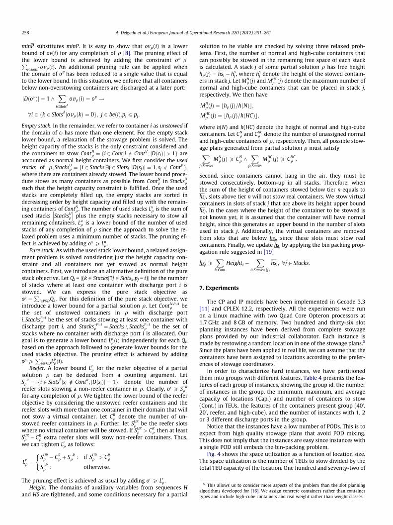
Fig. 4 shows the space utilization as a function of location size.The space utilization is the number of TEUs to stow divided by thetotal TEU capacity of the location. One hundred and seventy-two of

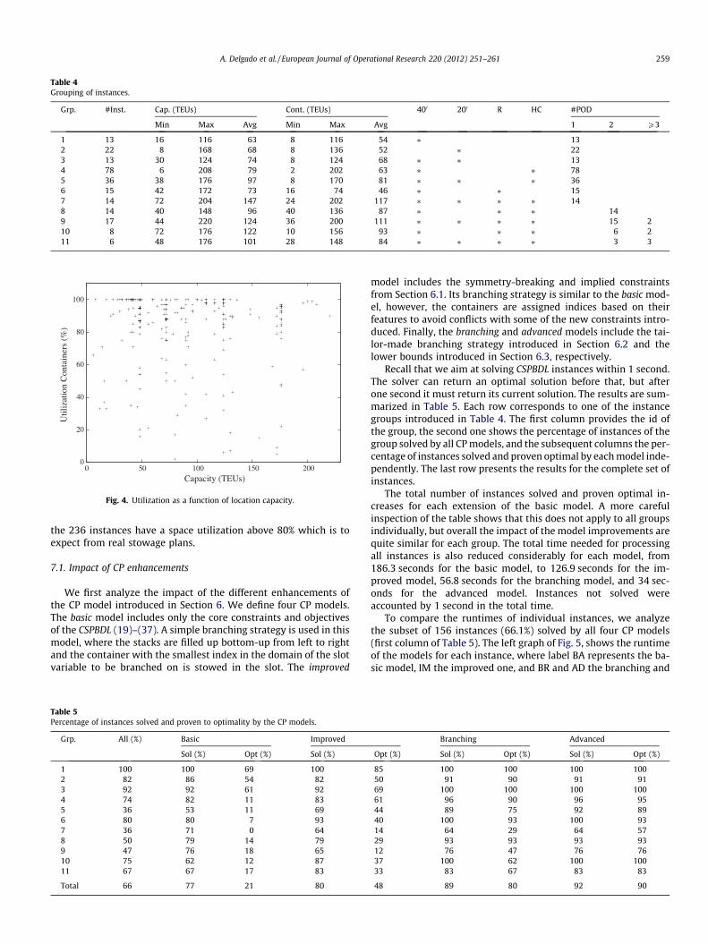
Table 4Grouping of instances.

Grp. #Inst. Cap. (TEUs) Cont. (TEUs) 400 200 R HC #POD

Min Max Avg Min Max Avg 1 2 P3

1 13 16 116 63 8 116 54 ⁄ 132 22 8 168 68 8 136 52 ⁄ 223 13 30 124 74 8 124 68 ⁄ ⁄ 134 78 6 208 79 2 202 63 ⁄ ⁄ 785 36 38 176 97 8 170 81 ⁄ ⁄ ⁄ 366 15 42 172 73 16 74 46 ⁄ ⁄ 157 14 72 204 147 24 202 117 ⁄ ⁄ ⁄ ⁄ 148 14 40 148 96 40 136 87 ⁄ ⁄ ⁄ 149 17 44 220 124 36 200 111 ⁄ ⁄ ⁄ ⁄ 15 210 8 72 176 122 10 156 93 ⁄ ⁄ ⁄ 6 211 6 48 176 101 28 148 84 ⁄ ⁄ ⁄ ⁄ 3 3

0

20

40

60

80

100

0 50 100 150 200

Util

izat

ion

Con

tain

ers

(%)

Capacity (TEUs)

Fig. 4. Utilization as a function of location capacity.

A. Delgado et al. / European Journal of Operational Research 220 (2012) 251–261 259

the 236 instances have a space utilization above 80% which is toexpect from real stowage plans.

7.1. Impact of CP enhancements

We first analyze the impact of the different enhancements ofthe CP model introduced in Section 6. We define four CP models.The basic model includes only the core constraints and objectivesof the CSPBDL (19)–(37). A simple branching strategy is used in thismodel, where the stacks are filled up bottom-up from left to rightand the container with the smallest index in the domain of the slotvariable to be branched on is stowed in the slot. The improved

Table 5Percentage of instances solved and proven to optimality by the CP models.

Grp. All (%) Basic Improved

Sol (%) Opt (%) Sol (%)

1 100 100 69 1002 82 86 54 823 92 92 61 924 74 82 11 835 36 53 11 696 80 80 7 937 36 71 0 648 50 79 14 799 47 76 18 6510 75 62 12 8711 67 67 17 83

Total 66 77 21 80

model includes the symmetry-breaking and implied constraintsfrom Section 6.1. Its branching strategy is similar to the basic mod-el, however, the containers are assigned indices based on theirfeatures to avoid conflicts with some of the new constraints intro-duced. Finally, the branching and advanced models include the tai-lor-made branching strategy introduced in Section 6.2 and thelower bounds introduced in Section 6.3, respectively.

Recall that we aim at solving CSPBDL instances within 1 second.The solver can return an optimal solution before that, but afterone second it must return its current solution. The results are sum-marized in Table 5. Each row corresponds to one of the instancegroups introduced in Table 4. The first column provides the id ofthe group, the second one shows the percentage of instances of thegroup solved by all CP models, and the subsequent columns the per-centage of instances solved and proven optimal by each model inde-pendently. The last row presents the results for the complete set ofinstances.

The total number of instances solved and proven optimal in-creases for each extension of the basic model. A more carefulinspection of the table shows that this does not apply to all groupsindividually, but overall the impact of the model improvements arequite similar for each group. The total time needed for processingall instances is also reduced considerably for each model, from186.3 seconds for the basic model, to 126.9 seconds for the im-proved model, 56.8 seconds for the branching model, and 34 sec-onds for the advanced model. Instances not solved wereaccounted by 1 second in the total time.

To compare the runtimes of individual instances, we analyzethe subset of 156 instances (66.1%) solved by all four CP models(first column of Table 5). The left graph of Fig. 5, shows the runtimeof the models for each instance, where label BA represents the ba-sic model, IM the improved one, and BR and AD the branching and

Branching Advanced

Opt (%) Sol (%) Opt (%) Sol (%) Opt (%)

85 100 100 100 10050 91 90 91 9169 100 100 100 10061 96 90 96 9544 89 75 92 8940 100 93 100 9314 64 29 64 5729 93 93 93 9312 76 47 76 7637 100 62 100 10033 83 67 83 83

48 89 80 92 90

0

0.2

0.4

0.6

0.8

1

0 20 40 60 80 100 120 140

time

(s)

instance

BAIMBRAD

0

100

200

300

400

500

0 5 10 15 20 25 30 35

optim

ality

gap

(%

)

instance

BAIMBR

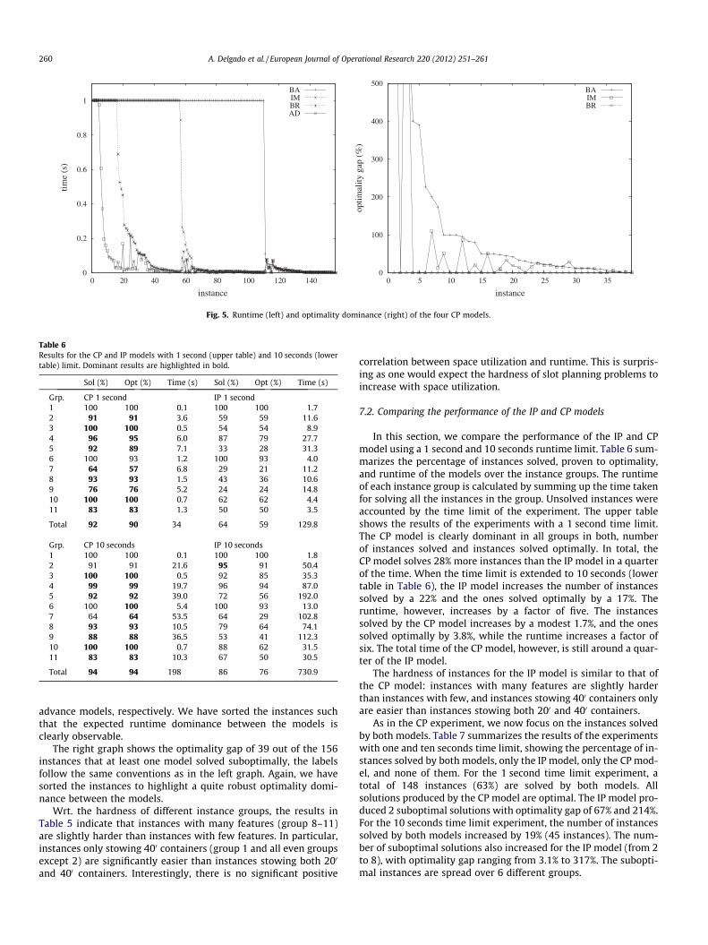
Fig. 5. Runtime (left) and optimality dominance (right) of the four CP models.

Table 6Results for the CP and IP models with 1 second (upper table) and 10 seconds (lowertable) limit. Dominant results are highlighted in bold.

Sol (%) Opt (%) Time (s) Sol (%) Opt (%) Time (s)

Grp. CP 1 second IP 1 second1 100 100 0.1 100 100 1.72 91 91 3.6 59 59 11.63 100 100 0.5 54 54 8.94 96 95 6.0 87 79 27.75 92 89 7.1 33 28 31.36 100 93 1.2 100 93 4.07 64 57 6.8 29 21 11.28 93 93 1.5 43 36 10.69 76 76 5.2 24 24 14.810 100 100 0.7 62 62 4.411 83 83 1.3 50 50 3.5

Total 92 90 34 64 59 129.8

Grp. CP 10 seconds IP 10 seconds1 100 100 0.1 100 100 1.82 91 91 21.6 95 91 50.43 100 100 0.5 92 85 35.34 99 99 19.7 96 94 87.05 92 92 39.0 72 56 192.06 100 100 5.4 100 93 13.07 64 64 53.5 64 29 102.88 93 93 10.5 79 64 74.19 88 88 36.5 53 41 112.310 100 100 0.7 88 62 31.511 83 83 10.3 67 50 30.5

Total 94 94 198 86 76 730.9

260 A. Delgado et al. / European Journal of Operational Research 220 (2012) 251–261

advance models, respectively. We have sorted the instances suchthat the expected runtime dominance between the models isclearly observable.

The right graph shows the optimality gap of 39 out of the 156instances that at least one model solved suboptimally, the labelsfollow the same conventions as in the left graph. Again, we havesorted the instances to highlight a quite robust optimality domi-nance between the models.

Wrt. the hardness of different instance groups, the results inTable 5 indicate that instances with many features (group 8–11)are slightly harder than instances with few features. In particular,instances only stowing 400 containers (group 1 and all even groupsexcept 2) are significantly easier than instances stowing both 200

and 400 containers. Interestingly, there is no significant positive

correlation between space utilization and runtime. This is surpris-ing as one would expect the hardness of slot planning problems toincrease with space utilization.

7.2. Comparing the performance of the IP and CP models

In this section, we compare the performance of the IP and CPmodel using a 1 second and 10 seconds runtime limit. Table 6 sum-marizes the percentage of instances solved, proven to optimality,and runtime of the models over the instance groups. The runtimeof each instance group is calculated by summing up the time takenfor solving all the instances in the group. Unsolved instances wereaccounted by the time limit of the experiment. The upper tableshows the results of the experiments with a 1 second time limit.The CP model is clearly dominant in all groups in both, numberof instances solved and instances solved optimally. In total, theCP model solves 28% more instances than the IP model in a quarterof the time. When the time limit is extended to 10 seconds (lowertable in Table 6), the IP model increases the number of instancessolved by a 22% and the ones solved optimally by a 17%. Theruntime, however, increases by a factor of five. The instancessolved by the CP model increases by a modest 1.7%, and the onessolved optimally by 3.8%, while the runtime increases a factor ofsix. The total time of the CP model, however, is still around a quar-ter of the IP model.

The hardness of instances for the IP model is similar to that ofthe CP model: instances with many features are slightly harderthan instances with few, and instances stowing 400 containers onlyare easier than instances stowing both 200 and 400 containers.

As in the CP experiment, we now focus on the instances solvedby both models. Table 7 summarizes the results of the experimentswith one and ten seconds time limit, showing the percentage of in-stances solved by both models, only the IP model, only the CP mod-el, and none of them. For the 1 second time limit experiment, atotal of 148 instances (63%) are solved by both models. Allsolutions produced by the CP model are optimal. The IP model pro-duced 2 suboptimal solutions with optimality gap of 67% and 214%.For the 10 seconds time limit experiment, the number of instancessolved by both models increased by 19% (45 instances). The num-ber of suboptimal solutions also increased for the IP model (from 2to 8), with optimality gap ranging from 3.1% to 317%. The subopti-mal instances are spread over 6 different groups.

Table 7Results for the instances solved by any of the two models with one and 10 seconds time limit.

Grp. 1 second 10 seconds

Both (%) IP (%) CP (%) None (%) Both (%) IP (%) CP (%) None (%)

1 100 0 0 0 100 0 0 02 55 5 35 5 82 14 4 03 54 0 46 0 92 0 8 04 86 1 10 3 95 1 4 05 33 0 58 9 67 6 24 36 100 0 0 0 100 0 0 07 29 0 36 35 50 14 22 148 43 0 50 7 71 8 21 09 24 0 53 24 53 0 35 1210 62 0 38 0 88 0 12 011 50 0 33 17 67 0 17 16Tot 63 1 29 7 82 4 11 3

A. Delgado et al. / European Journal of Operational Research 220 (2012) 251–261 261

8. Conclusion

In this paper, we have introduced an accurate definition calledCSPBDL of stowing a set of containers in a bay section. The CSPBDLis NP-hard and is an important sub-problem of the successful mul-ti-phase approaches to stowage planning optimization. We havedeveloped two CP and IP models to solve the CSPBDL optimally.Our computationally results show that both models can be solvedfast and that it is possible to improve the performance of the CPmodel such that it can produce optimal solutions for 90% of 236industrial instances in less than 1 second, which is well withinthe time requirements for practical stowage support tools. Futureresearch includes improving the performance and stability of oursolvers (e.g., diving heuristics and other techniques may be usedto improve the IP model) and extending the CSPBDL to include ondeck locations and special containers such as out-of-gauge, pal-let-wide, and containers with dangerous goods.

Acknowledgements

We would like to thank the anonymous reviewers and the fol-lowing academic and industrial collaborators: Christian Schulte,Mikael Lagerkvist, Thomas Stidsen, Jon Freeman, Robert John Mil-ton, Nicolas Guilbert, Kim Hansen, and Thomas Bebbington. Thisresearch was partly funded by The Council for Strategic Research,within the programme ‘‘Green IT’’.

References

[1] D. Ambrosino, D. Anghinolfi, M. Paolucci, A. Sciomachen, An experimentalcomparison of different heuristics for the master bay plan problem, in:Proceedings of the 9th International Symposium on Experimental Algorithms,2010, pp. 314–325.

[2] D. Ambrosino, A. Sciomachen, A constraint satisfaction approach for masterbay plans, Maritime Engineering and Ports 36 (1998) 175–184.

[3] D. Ambrosino, A. Sciomachen, D. Anghinolfi, M. Paolucci, A new three-stepheuristic for the master bay plan problem, Maritime Economics and Logistics11 (1) (2009) 98–120.

[4] A.H. Aslidis, Optimal container loading. Master’s thesis, MassachusettsInstitute of Technology, 1984.

[5] M. Avriel, M. Penn, N. Shpirer, Container ship stowage problem: complexityand connection to the coloring of circle graphs, Discrete Applied Mathematics103 (2000) 271–279.

[6] M. Avriel, M. Penn, N. Shpirer, S. Witteboon, Stowage planning for containerships to reduce the number of shifts, Annals of Operations Research 76 (1998)55–71.

[7] R. Botter, M.A. Brinati, Stowage container planning: a model for getting anoptimal solution, Proceedings of the IFIP TC5/WG5.6 Seventh InternationalConference on Computer Applications in the Automation of ShipyardOperation and Ship Design, vol. VII, North-Holland Publishing Co.,Amsterdam, The Netherlands, 1992, pp. 217–229.

[8] A. Delgado, R.M. Jensen, K. Janstrup, T.H. Rose, K.H. Andersen, A constraintprogramming model for fast optimal stowage of container vessel bays. Tech.Rep. TR-2010-133, IT University of Copenhagen, 2010.

[9] A. Delgado, R.M. Jensen, C. Schulte, Generating optimal stowage plans forcontainer vessel bays, in: Proceedings of the 15th International Conference onPrinciples and Practise of Constraint Programming (CP-09), Springer, 2009, pp.6–20.

[10] O. Dubrovsky, G.L.M. Penn, A genetic algorithm with a compact solutionencoding for the container ship stowage problem, Journal of Heuristics 8(2002) 585–599.

[11] Gecode Team, Gecode: Generic constraint development environment, 2006.<http://www.gecode.org>.

[12] N. Guilbert, B. Paquin, Container vessel stowage planning, Patent PublicationUS2010/0145501, 2010.

[13] P.V. Hentenryck, J.P. Carrillon, Generality vs. specificity: an experience with AIand OR techniques, in: Proceedings of the National Conference on ArtificialInteligence (AAAI), ACM press, 1988, pp. 660–664.

[14] J. Kang, Y. Kim, Stowage planning in maritime container transportation,Journal of the Operations Research Society 53 (4) (2002) 415–426.

[15] F. Li, C. Tian, R. Cao, W. Ding, An integer programming for container stowageproblem, in: Proceedings of the International Conference on ComputationalScience, Part I, LNCS, vol. 5101, Springer, 2008, pp. 853–862.

[16] D. Pacino, A. Delgado, R.M. Jensen, T. Bebbington, Fast generation of near-optimal plans for eco-efficient stowage of large container vessels, in:Proceedings of the Second International Conference on ComputationalLogistics (ICCL’11), Springer, 2011, pp. 286–301.

[17] G. Pesant, A regular language membership constraint for finite sequences ofvariables, in: Proceeding of Principles and Practice of Constraint Programming,Lecture Notes in Computer Science, vol. 3258, Springer, 2004, pp. 482–495.

[18] A. Sciomachen, A. Tanfani, The master bay plan problem: a solution methodbased on its connection to the three-dimensional bin packing problem, IMAJournal of Management Mathematics 14 (2003) 251–269.

[19] P. Shaw, A constraint for bin packing, in: Proceeding of Principles and Practiceof Constraint Programming, Lecture Notes in Computer Science, vol. 3258,Springer, 2004, pp. 648–662.

[20] B. Smith, Modelling, in: F. Rossi, P. van Beek, T. Walsh (Eds.), Handbook ofConstraint Programming, Elsevier, 2006. Chapter 11.

[21] I.D. Wilson, P. Roach, Container stowage planning: a methodology forgenerating computerised solutions, Journal of the Operational ResearchSociety 51 (11) (2000) 248–255.

[22] M. Yoke, H. Low, X. Xiao, F. Liu, S.Y. Huang, W.J. Hsu, Z. Li, An automatedstowage planning system for large containerships, in: Proceedings of the 4thVirtual International Conference on Intelligent Production Machines andSystems, 2009.

[23] W.-Y. Zhang, Y. Lin, Z.-S. Ji, Model and algorithm for container ship stowageplanning based on bin-packing problem, Journal of Marine Science andApplication 4 (3) (2005).