A Continuity Refinement for Rational Expectations Solutions

Bennett T. McCallum

Carnegie Mellon University

and

National Bureau of Economic Research

Preliminary

July 1, 2010, revised September 5, 2011

ABSTRACT: Linear RE models often have more than one dynamically stable solution. Consider, however, the requirement that the solution coefficients must be continuous in the model’s structural parameters. In particular, we require that the solutions should be continuous in the limit as those parameters, which express quantitatively the extent to which expectations affect endogenous variables, go to zero. The paper shows that under this condition there is, for a very broad class of linear RE models, only a single solution.

I am grateful to Seonghoon Cho, Robert Lucas, Albert Marcet, and Holger Sieg for helpful comments.

1

1. Introduction

It is very widely recognized that rational expectations (RE) models typically

feature a multiplicity of solutions, i.e., processes for endogenous variables that satisfy all

the model’s equations and the orthogonality conditions for RE. Various “selection

criteria” or “solution refinements” have been proposed over the years, by writers

including Blanchard and Kahn (1980), Whiteman (1983), McCallum (1983), Evans

(1986), Evans and Honkapohja (2001), Driskill (2006), and Cho and Moreno (2011).

None of these proposals, however, has been generally accepted by researchers. The most

prominent approach—that of Blanchard-Kahn and Whiteman—is to assume that if there

is only a single solution that is dynamically stable then it will prevail; otherwise each

stable solution represents a possible outcome. But it too has a number of critics, with

various objections being voiced by the other writers listed above plus Bullard (2006),

Bullard and Mitra (2002), and Cochrane (2007).1

In monetary economics the Blanchard-Kahn-Whiteman “determinacy” approach

is by far the most popular, partly due to the enormous influence of Woodford (2003, pp.

77-85, 90-96, 252-261). That the issues generated by solution multiplicities are central to

the logical foundations of today’s mainstream New-Keynesian approach to monetary

policy analysis, and that they remain unsettled, is clearly evidenced by the recent

exchange between Cochrane (2009) and McCallum (2009b).2 The purpose of the present

paper, consequently, is to propose a criterion or refinement, one that is based on

continuity of solution coefficients with respect to structural parameters. The spirit of the

1 It should be noted that the current revised version of Cochrane’s NBER Working Paper 13409, a version of which has been published as Cochrane (2011), has eliminated most of the discussion that is quoted critically in McCallum (2009b). 2 For a brief account, see Appendix C.

2

undertaking is that the objective in economic modelling is not primarily to conform to

some particular definition of equilibrium, but to develop models that are plausible, in

terms of their predictions about the consequences of alternative economic arrangements

and policies. Throughout the present discussion, the analysis will be limited to linear

models.

2. Basic Univariate Case

Consider the following univariate model, assumed to be structural:

(1) t t t 1 t 1y aE y cy ac 0.25 .

Here we have for simplicity omitted the constant term and exogenous shocks, which are

inessential to the argument.3 The “fundamental” solutions are of the form

(2) t t 1y y

so 2t t 1 t 1E y y . Then substitution of the latter and (2) into (1) followed by

undetermined-coefficient (UC) reasoning indicates that must satisfy

(3) 2a c 0 .

Thus the fundamental solutions are given by (2) with the following two values for :

(4a) ( ) 1 1 4ac

2a

(4b) ( ) 1 1 4ac

2a

.

The proposed refinement is that must be continuous in the parameters a and c.

In particular, must be continuous in ‘a’ over intervals of values that include a = 0. The

rationale is that in this extreme case expectational variables are absent from the model so

3 With respect to exogenous variables, see Appendix A. Note that condition ac<1 is to give real-valued solutions.

3

the solution is unambiguously t t 1y cy . In addition, small values of ‘a’ reflect cases in

which expectational effects are small, so they should imply solutions with close to c.

Furthermore, continuity of solution parameters is necessary for impulse-response

functions to be well behaved when exogenous variables are included in the model.4

Clearly, this requirement implies that the solution for model (1) is given by (2)

with the limiting value, as a 0 , of ( ) = c, as in (4a), and not by ( ) , i.e., an

infinite discontinuity.5 It is useful to note that (with a 0 ) as the parameter c 0 we

have ( ) 0 , whereas ( ) 1/ a . Thus the refinement leads to the same solution as

the minimum state variable (MSV) solution suggested by McCallum (1983).

From the foregoing we see that the proposed refinement leads to a single solution

when we are limiting consideration to fundamental solutions. But suppose we admit

solutions of the general “sunspot” form

(5) t 1 t 1 2 t 2 3 ty y y ,

where t is a stationary stochastic process with the property t t 1E = 0.6 Then we have

(6) t t 1 1 1 t 1 2 t 2 3 t 2 t 1E y ( y y ) y 0

and substitution into (1) leads to the following UC conditions:

(7a) 21 1 2a a c

(7b) 2 1 2a

(7c) 3 1 3a .

Now, the last two of these require that either a1 = 1 or that 2 = 3 = 0. In the latter case

4 Again see Appendix A. 5 The first of the two limits is obtained by means of l’Hôpital’s rule; see Appendix A. 6 It is the case that any RE solution to model (1) can be expressed in this form. See, e.g., Lubik and Schorfheide (2003).

4

we have the same fundamental solutions as before, but in the former case 3 can be any

real number and then (7a) reduces to

(8) 2

1 1a c

a a ,

that is, to 2 = c/a, which is not contradicted by (7b). So there is a sunspot solution

(9) t t 1 t 2 3 t

1 cy y y

a a

for any finite value of 3. Clearly, however, the solution coefficients in (9) are not

continuous at a = 0.7 So the proposed refinement rules out all solutions except (2) with

given by ( ) . Obviously, to be useful this result must extend to richer models. Even in

the present context, however, it is interesting that there is only a single solution that

satisfies the continuity principle. More significantly, perhaps, it is the same solution as

the one that utilizes a “direction of causality” criterion as developed in McCallum

(2009a), as well as the “minimum state variable” solution from McCallum (1983).8

One reader has asked why an analyst should be concerned with properties

( ) prevailing in the vicinity of a = 0 in cases in which it is likely that ‘a’ is not close to 0

(e.g., the model has a = 0.95). My response is that what we are concerned with at this

methodological step is whether the solution with ( ) or the one with ( ) is appropriate

for models of the specification at hand. Thus we ask whether the functions ( ) and ( )

imply plausible solutions for all values of ‘a’ and c that are permitted by the model (here,

all values such that ac<0.25). For example, how would the two solutions (functions of a

7 The coefficient on yt-1 in (9) implies that a tiny change in the expectational parameter a—say, from 0.01 to 0.01—could have an implausibly large effect on the dynamic behavior of yt.8 The latter has been recognized as a notable concept by several writers, including Evans and Honkapohja (2001), Driskill (2006), and Cho and Moreno (2011).

5

and c) behave in the case that a = 0.01? And the case that a = 0.01? Clearly the

solution ( ) says that ϕ would be huge and positive in one case but huge and negative in

the other. It is implausible, I suggest, that this small change in model calibration could

have such huge effects on the implied economic behavior of variable yt, especially since

the small absolute value of ‘a’ in both cases indicates that for prices or quantities the

effects of expectations about the next-period values should have very little effect—as is,

in fact, implied by the solution ( ) . Methodologically, it is appropriate to decide which

solution function is appropriate before turning to the specific parameter values relevant to

the economy at hand, ‘a’ and c, for the applied step of forecasting or policy analysis.

Multivariate Extension

We now consider richer models of the form

(10) yt = A Etyt+1 + C yt-1 + D ut,

where yt is a m×1 vector of endogenous variables, A and C are m×m matrices of real

numbers, D is mn, and ut is a n×1 vector of exogenous variables generated by a

dynamically stable process

(11) ut = Rut-1 + εt,

with εt a white noise vector and R a matrix with all eigenvalues less than 1.0 in modulus.

It will not be assumed that A is invertible. In this formulation the endogenous variables

in yt are jump variables whereas their lagged values in yt-1 are predetermined, that is,

dependent only on lagged values of exogenous or endogenous variables. This

specification is useful for various reasons, the main one with respect to the issue at hand

being that it is very broad and inclusive. In particular, any model satisfying the

formulations of King and Watson (1998) or Klein (2001), can (with the use of auxiliary

6

variables) be written in this form—and the form will accommodate any finite number of

lags, expectational leads, and lags of expectational leads.9 In that context, we consider

fundamental solutions to the model (10)-(11), which are of the form

(12) yt = Ω yt-1 + Γ ut.

in which is required to be real.10 Then we have that Etyt+1 = (yt-1 + ut) + Rut and

straightforward undetermined-coefficient reasoning shows that and must satisfy

(13) A2 + C = O

(14) = A + AR + D.

For any given , (14) yields a unique generically,11 but there may be many mm real

matrices that solve (13) for . Accordingly, the following analysis centers around (13),

setting D = O for simplicity. For reference below, note that, from (13), each solution will

satisfy

(15) 1(I A ) C ,

provided that the inverse exists.

In order to accommodate singular A matrices, we write

(16) A

0

O

I

2

= I

I

C

O

I

,

in which the first row reproduces the matrix quadratic (13). Let the 2m2m matrices on

the left and right sides of (16) be denoted A and C , respectively. Then we solve for the

(generalized) eigenvalues of the matrix pencil [C A] , alternatively termed the

9 See McCallum (2007, p. 1379). 10 A constant term can be defined by the coefficient on an exogenous variable that is a driftless random walk with innovation variance of zero. 11 Generically, I R[(I A)-1A] will be invertible, permitting solution for vec() using the identity vec(ABC) = [CA]vec(B) that holds for any conformable A, B, and C.

7

(generalized) eigenvalues of C with respect to A (e.g., Uhlig (1999)). Specifically, the

Schur generalized decomposition theorem establishes that there exist unitary matrices Q

and Z of order 2m2m such that QCZ = T and QAZ = S with T and S triangular.12

Then eigenvalues of the matrix pencil [C A] are defined as tii/sii. Some of these

eigenvalues may be “infinite,” in the sense that some sii may equal zero. This will be the

case, indeed, whenever A and therefore A are of less than full rank since then S is also

singular. All of the foregoing is true for any ordering of the eigenvalues and associated

columns of Z (and rows of Q). For the moment, let us temporarily focus on the

arrangement that places the tii/sii in order of decreasing modulus, which will be referred to

as the MOD ordering.13

To begin the analysis, premultiply (16) by Q. Since QA = SH and QC = TH,

where H Z-1, the resulting equation can be written as

(17) 11

21

S

S

22

O

S

11

21

H

H

12

22

H

H

2

= 11

21

T

T

22

O

T

11

21

H

H

12

22

H

H

I

.

The first row of (17) reduces to

(18) S11(H11 + H12) = T11(H11 + H12).

Then if H11 is invertible the latter can be used to solve for , which is mm, as

(19) = H11-1

H12 =

where the second equality uses the upper right-hand submatrix of the identity HZ = I,

12 Provided only that there exists some for which det[ C A ] 0. See Klein (2000) or Golub and Van Loan (1996). 13 The discussion proceeds as if none of the tii/sii equals 1.0 exactly. If one does, the model can be adjusted, by multiplying some relevant coefficient by (e.g.) 0.9999 or eliminating the variable in favor of its first difference.

8

provided that H11 is invertible, which we assume without significant loss of generality.14

As mentioned above, there are many fundamental solutions to (13). These

correspond to the (2m)!/(m!)2 different combinations of the 2m eigenvalues taken m at a

time, which result in different groupings of the columns of Z and therefore different

compositions of the submatrices Z12 and Z22. Here, with the eigenvalues tii/sii temporarily

arranged in order of decreasing modulus, the diagonal elements of S22 will all be non-

zero provided that S has at least m non-zero eigenvalues, which we assume to be the

case.15 For any solution under consideration to be dynamically stable, all the eigenvalues

of must of course be smaller than 1.0 in modulus. To evaluate them in terms of the

ratios tii/sii, note that with given by (19), the second row of (17) becomes

(20) S22(H21 + H22) = T22(H21 + H22),

or

(21) S22(H22 H12) = T22(H22

H12).

The latter, by virtue of the lower right-hand submatrix of HZ = I, is equivalent to

(22) S22 = T22Z22

1.

Therefore we have the result

(23) = Z22S22-1T22Z22

1,

so has the same eigenvalues as S22-1T22. The latter is triangular, moreover, so the

relevant eigenvalues are (given the MOD ordering) the m smallest of the 2m ratios tii/sii.

For dynamic stability, the modulus of each of these ratios must then be less than 1. (In

14 This invertibility condition, also required by King and Watson (1998) and Klein (2000), obtains except for degenerate special cases of (1) that can be solved by simpler methods than considered here. Note that the invertibility of H11 implies the invertibility of Z22, given that H and Z are unitary. 15 It is obvious that A has at least m nonzero eigenvalues so, with Q and Z unitary, S must have rank of at least m. This is not sufficient for S to have at least m nonzero eigenvalues, however; hence the assumption.

9

many cases, some of the m smallest moduli will equal zero.)

Next we consider alternative fundamental solutions, which will involve departures

from the MOD ordering. There are (2m)!/(m!)2 different groupings of system

eigenvalues (and associated eigenvectors) that include two groups of m each. It is well

known (and is shown in (23)) that m of the system eigenvalues will be the eigenvalues of

. The other half of the system eigenvalues are those of the matrix 1F , where

1F (I A ) A .16 According to our refinement, we now select the solution for which

C as A O . By continuity of eigenvalues with respect to structural parameters

(Horn and Johnson, 1985, pp. 539-540), this is the same solution as the MSV solution for

which O as C O .17 It can be identified operationally by replacing C by C in all

equations and then letting the scalar decrease continuously from 1 to 0. Examination of

a plot or table of the eigenvalues for various values will indicate which solution—i.e.,

which —has this property. [This procedure is mentioned in McCallum (2004) and

illustrated in McCallum (2009a).] Let us use 0 to denote the matrix for this particular

solution, with the related F matrix being 10 0F (I A ) A . Furthermore, we observe

crucially that any other fundamental solution will have one or more of the eigenvalues of

Ω approaching ±∞ as A →O. See Appendix B. Thus we have developed the multivariate

extension of the argument for fundamentals solutions.

It is important to note that the Ω0, F0 solution does not necessarily coincide with

the MOD solution. In most cases these two solutions will coincide, but in some cases

they differ. This fact, which is mentioned by Uhlig (1999, p. 46), is illustrated in 16 This result, which is somewhat tedious, is developed in McCallum (2007, pp. 1382-3). 17 This generalization of the univariate case regarding (4a) and (4b) is implied by the analysis on p. 165 of McCallum (1983), with extension to singular A matrices by noting that they imply eigenvalues of F equal to zero. For details, see Appendix B.

10

McCallum (2004) and (2009a).18

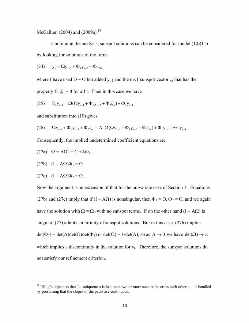
Continuing the analysis, sunspot solutions can be considered for model (10)(11)

by looking for solutions of the form

(24) t t 1 1 t 2 2 ty y y

where I have used D = O but added yt-2 and the m1 sunspot vector t that has the

property Et-1t = 0 for all t. Then in this case we have

(25) t t 1 t 1 1 t 2 2 t 1 t 1E y ( y y ) y

and substitution into (10) gives

(26) t 1 1 t 2 2 ty y = A[ t 1 1 t 2 2 t 1 t 1( y y ) y ] + t 1Cy .

Consequently, the implied undetermined coefficient equations are

(27a) = A2 + C +A1

(27b) (I A)1 = O

(27c) (I A)2 = O.

Now the argument is an extension of that for the univariate case of Section 3. Equations

(27b) and (27c) imply that if (I A) is nonsingular, then 1 = O, 2 = O, and we again

have the solution with = 0 with no sunspot terms. If on the other hand (I A) is

singular, (27) admits an infinity of sunspot solutions. But in this case (27b) implies

det(1) = det(A)det()det(1) or det() = 1/det(A), so as A 0 we have det( )

which implies a discontinuity in the solution for yt. Therefore, the sunspot solutions do

not satisfy our refinement criterion.

18 Uhlig’s objection that “…uniqueness is lost once two or more such paths cross each other …” is handled by presuming that the slopes of the paths are continuous.

11

4. Conclusion

We conclude with a very brief description of the paper’s argument. Linear RE

models typically have more than one solution and fairly often possess more than one

dynamically stable solution. Consider, however, the requirement that the solution

coefficients should be continuous in the model’s structural parameters. In particular, we

require that the solution coefficients should be continuous in the limit as certain

parameters, which express the extent to which expectations affect endogenous variables,

go to zero. (If expectations enter the structural equations very weakly, they should not

have much effect on the solution expressions.) The paper shows that, for a very broad

class of linear RE models,19 this requirement is satisfied by only a single solution.

19 The class is one that permits any finite (i) number of endogenous variables, (ii) lag length, (iii) expectational lead length, and (iv) lag length for expectational leads.

12

Appendix A

The purpose here is to illustrate that it is sufficient for this paper’s argument to

examine cases in which exogenous variables are not explicitly included. For the simplest

case, suppose that we extend equation (1) to include an exogenous shock zt that is

generated by a stable first-order autoregressive process with coefficient ρ. Then we have

(A-1) t t t 1 t 1 ty aE y cy dz

(A-2) t t 1 tz z

where εt is white noise. Then fundamental solutions are of the form

(A-3) yt = 1yt-1 + ϕ2zt.

Consequently, 2t t 1 1 t 1 1 2 tE y y ( ) z . Using the latter and (A-3) in (A-1) we have

(A-4) 21 t 1 2 t 1 t 1 2 1 t t 1 ty z a[ y ( )z ] cy dz

so equating coefficients yields

(A-5) 21 1a c

(A-6) 2 2 1a ( ) d .

As in Section 2, therefore, from (A-5) we have

(A-7a) ( )1

1 1 4ac

2a

(A-7b) ( )1

1 1 4ac

2a

.

Thus as a 0 we have ( )1 c and ( )

1 as with equations (4a) and (4b).20

Continuing, for ( )2 we have ( ) ( )

2 1[1 a a ] d or ( ) ( )2 1d / [1 a a ]

20 In the case of (A-7a), both numerator and denominator approach zero as a approaches zero, but their derivatives approach 2c and 2 respectively, so L’Hospital’s rule gives a limit of c.

13

so that ( )2

d

1 1 4ac1 a

2

and

(A-8) ( )2

a 0

dlim d

1 11 0

2

Whereas ( )2a 0

dlim

1 11 0

2

Next, the non-fundamental solutions—permitting sunspots—are of form

(A-9) t 1 t 1 2 t 3 t 1 4 ty y z z

for any t with t 1 tE 0. Then t t 1 1 1 t 1 2 t 3 t 1 4 t 2 t 3 tE y ( y z z ) z z 0

whereby substitution into (A-1) plus equating of coefficients yields

(A-10) 21 1a

(A-11) 2 1 2 2 1 3d a a a

(A-12) 3 1 3a

(A-13) 4 1 4a

Thus we have either 1 3 4 0 in which case 2 d / (1 a ) and yields the well-

behaved MSV solution (2) with (4a); or else we have 1 1/ a in which case

2 3(d ) / a and thus for any arbitrary ϕ3 (except the zero-measure value of d)

there is an infinite discontinuity in the limit as a 0 . Accordingly, permitting sunspot

solutions does not alter the conclusion that only the MSV solution avoids the implication

of an infinite discontinuity in the implied impulse response function.

14

Appendix B

The object here is to show that the solution (12) to model (10)(11) for which

C as A O is the same solution as the one for which O as C O . Let us

begin with the case in which A is nonsingular. Then we can express the crucial matrix

quadratic (13) as

(B-1) 2

=

1A

I

1A C

O

I

.

Let M denote the square matrix of order 2m × 2m. Clearly its eigenvalues are the

numbers denoted that satisfy

(B-2) det(M I) = det 1A I

I

1A C

O I

= 0.

An identity for partitioned matrices reported by Johnston (1972, eqn. 4-37, p. 95) is as

follows. If the matrix 11 12

21 22

B BB

B B

with B11 nonsingular, then

(B-3) det(B) = det(B11) 1

22 21 11 12det[B B B B ] .

The latter then implies that

(B-4) det(M I) = 1det(A I) 1 1 1det[ I (A I) A C] 0.

Thus we see, from the latter, that half of the eigenvalues of M are the eigenvalues of A1,

while the other half, the eigenvalues of , depend upon both A and C (see McCallum

2007, pp. 1382-3). Then by further inspection of (B-4) we see that when C = O, the

second half of the s are all equal to 0. Thus the single solution given by the particular

arrangement for which all eigenvalues of approach zeros as C O , simultaneously

has the other half of the eigenvalues of M approaching the eigenvalues of A1.

15

. Now consider the same arrangement but with C held fixed and consider the

implication of A O . Then the eigenvalues that approached zeros before now approach

the eigenvalues of C while the eigenvalues that approached those of A1 before now

approach ± . This establishes the result at issue for the case in which A is nonsingular.

For any other solution—any other arrangement—as A→O we would have a different Ω

and one or more of its eigenvalues would approach ± .

When instead A is singular, similar results obtain but with the matrix A being

replaced in the argument by the matrix F = (I A)1A.21 The system eigenvalues then

include those of F1 and , instead of those of A1 and . As C O , we have the m

eigenvalues of approaching zeros and the other m eigenvalues approaching those of

F1 . Then with the same arrangement, i.e., the solution such that the eigenvalues of Ω

approach zeros as we C O , we find that as A O the eigenvalues of F1 each

approach ± .

21 Again, see McCallum (2007, pp. 1381-1383) for this result.

16

Appendix C

In recent monetary policy analysis, it has been common practice to view models

as possessing determinacy if they feature a single RE solution that is dynamically stable.

Cochrane (2007) has emphasized that this single-stable-solution (SSS) condition is not

sufficient as a criterion of determinacy, however, because in typical New Keynesian

models, if the Taylor Principle is satisfied, there exists a dynamically explosive solution

that is not ruled out by any transversality condition and accordingly can be eliminated

only by an arbitrary dictum. McCallum (2009b) agrees with this specific proposition, but

shows that in these models it is typically the case that the explosive solutions in question

are not least-squares learnable. Further, he argues that such learnability should be

considered a necessary condition for a solution to be regarded as a model’s prediction of

the depicted economy’s behavior since it amounts to a feasibility condition that pertains

to quantitative information available to individual agents.22 Consequently, he argues that,

despite Cochrane’s important point, the solution typically utilized in recent policy

analysis is in many (but not all) cases the appropriate one. Cochrane’s (2009) response

contends that there are three weaknesses in McCallum’s argument. McCallum’s (2009c)

rejoinder claims that in all three cases Cochrane’s argument is analytically incorrect or

inapplicable, as follows. First, the presence of unobserved exogenous shocks does not, in

contrast to Cochrane’s presumption, overturn learnability conclusions.23 Second,

Cochrane’s argument about “hyperinflationary threats” is not consistent with the

analytical setting in which the argument is normally conducted, namely, one in which the

central bank is following a specified policy rule for an interest-rate instrument. Third, the

22 See the discussion in McCallum (2011). 23 This is established in McCallum (2009b) by drawing on results of Evans and Honkapohja (1998).

17

point that a particular structural parameter, concerning the central bank’s policy behavior,

is not identifiable by an econometrician studying the economy-plus-policy process is not

relevant to the learning process for the private-sector agents in the model. Their learning

concerns forecasting of inflation and output in the model economy from a reduced form

perspective; the identification of a structural parameter by these agents is not necessary

for this step.

In his revised WP13409 and (2011), Cochrane emphasizes a distinct argument to

the effect that the reasoning utilized by Clarida, Gali, and Gertler (2000), among others,

who contend that empirical estimates show that the Taylor Principle was not satisfied in

the United States during the “Great Inflation” period of the 1970s, is invalid because the

crucial policy parameter is not identified. I agree with this significant point as applied to

the particular studies discussed by Cochrane, but withhold judgment on the universality

of this non-identification.

18

References

Blanchard, O.J., and C.M. Kahn.“The Solution of Linear Difference Models

Under Rational Expectations,” Econometrica 48, 1980, 1305-1311.

Bullard, J.B. “The Learnability Criterion and Monetary Policy,” Federal Reserve Bank of

St Louis Review 88(3),2006, 203-217.

Bullard, J.B., and K. Mitra, “Learning About Monetary Policy Rules,” Journal of

Monetary Economics 49, 2002, 1105-1129.

Cho, S., and Moreno, A. “The Forward Method as a Solution Refinement in Rational

Expectations Models,” Journal of Economic Dynamics and Control 35, 2011,

257-272.

Cochrane, J. H., “Inflation Determination with Taylor Rules: A Critical Review.” NBER

Working Paper 13409, 2007.

Cochrane, J.H., “Can Learnability Save New-Keynesian Models?” Journal of Monetary

Economics 56, 2009, 1109-1103.

Cochrane, J.H., “Determinacy and Identifiability in New Keynesian Models,” Journal of

Political Economy 2011.

Driskill, R. “Multiple Equilibria in Dynamic Rational Expectations Models: A Critical

Review,” European Economic Review 50, 2006, 171-210.

Evans, G.W., “Selection Criteria for Models with Non-uniqueness,” Journal of

Monetary Economics 18, 1986, 147-157.

Evans, G.W., and S. Honkapohja. Learning and Expectations in Macroeconomics.

Princeton Univ. Press, 2001.

Golub, G.H., and C.F. VanLoan. Matrix Computations, 3rd ed. Johns Hopkins

19

University Press, 1996.

Horn, R.A., and C. R. Johnson. Matrix Analysis. Cambridge University Press, 1985.

Johnston, J. Econometric Methods, 2nd ed. McCraw-Hill, 1972.

King, R.G., and M.W. Watson. “The Solution of Singular Linear Difference Systems

Under Rational Expectations,” International Economic Review 39, 1998, 1015-26.

Klein, P. “Using the Generalized Schur Form to Solve a Multivariate Linear

Rational Expectations Model,” Journal of Economic Dynamics and Control 24,

2000, 1405-1423.

Lubik, T.A., and F. Schorfheide. “Computing Sunspot Equilibria in Linear Rational

Expectations Models,” Journal of Economic Dynamics and Control 28, 2003,

273-285.

McCallum, B.T. “On Nonuniqueness in Linear Rational Expectations Models: An

Attempt at Perspective,” Journal of Monetary Economics 11, 1983, 139-168.

______________“On the Relationship Between Determinate and MSV Solutions

in Linear RE Models,” Economics Letters 84, 2004, 55-60.

_____________. “E-stability vis-a-vis Determinacy Results for a Broad Class of

Linear Rational Expectations Models,” Journal of Economic Dynamics and

Control 31, 2007, 1376-1391.

_____________. “Causality, Structure, and the Uniqueness of Rational Expectations

Equilibria,” NBER Working Paper 15234, August 2009(a). Also Manchester

School 79, 2011, 551-566.

_____________. “Inflation Determination with Taylor rules: Is New-Keynesian Analysis

20

Critically Flawed?” Journal of Monetary Economics 56, 2009(b), 1101-1108.

____________. “Rejoinder to Cochrane,” Journal of Monetary Economics 56, 2009(c),

1114-1115.

____________. “Issues Concerning Determinacy, Learnability, Plausibility, and the Role of Money in New Keynesian Models,” working paper, July 2011. Uhlig, H. “A Toolkit for Analyzing Nonlinear Dynamic Stochastic Models Easily,”

in Computational Methods for the Study of Dynamic Economies, R. Marimon

and A. Scott, eds. Oxford University Press, 1999.

Whiteman, C., Linear Rational Expectations Models: A User’s Guide. University of

Minnesota Press, 1983.

Woodford, M., Interest and Prices: Foundations for a Theory of Monetary Policy.

Princeton University Press, 2003.