A continuum limit for non-dominated sortingJeff Calder

Department of MathematicsUniversity of Michigan

Ann Arbor, MI 48109, USAEmail: jcalder@umich.edu

Selim EsedogluDepartment of Mathematics

University of MichiganAnn Arbor, MI 48109, USAEmail: esedoglu@umich.edu

Alfred O. Hero IIIDepartment of Electrical Engineering andComputer Science, University of Michigan

Ann Arbor, MI 48109, USAEmail: hero@eecs.umich.edu

Abstract— Non-dominated sorting is an important combinato-rial problem in multi-objective optimization, which is ubiquitousin many fields of science and engineering. In this paper, weoverview the results of some recent work by the authors ona continuum limit for non-dominated sorting. In particular, wehave discovered that in the (random) large sample size limit,the non-dominated fronts converge almost surely to the level setsof a function that satisfies a Hamilton-Jacobi partial differentialequation (PDE). We show how this PDE can be used to designa fast, potentially sublinear, approximate non-dominated sortingalgorithm, and we show the results of applying the algorithm toreal data from an anomaly detection problem.

Keywords: Non-dominated sorting, Pareto-optimality,multi-objective optimization, longest chain problem, antichainpartition, partial differential equations, Hamilton-Jacobiequations, numerical schemes

I. INTRODUCTION

Non-dominated sorting is an important combinatorial prob-lem in multi-objective optimization [1], [2], [3], [4]. Thesorting can be viewed as arranging points in Euclidean spaceinto layers, or fronts, by repeated removal of the set of minimalelements with respect to a partial order. It is an essentialstep in the so-called genetic and evolutionary algorithms forcontinuous multi-objective optimization, where it is employedto determine fitness levels of feasible solutions in the currentpopulation [3], [5], [6], [2], [7]. Of course, multi-objectiveoptimization is ubiquitous in many fields of science andengineering, including control theory and path planning [8],[9], [10], gene selection and ranking [11], [12], [13], [14],[15], [16], [17], data clustering [18], database systems [19],[20] and image processing and computer vision [21], [22].

In probability theory, non-dominated sorting goes by thepseudonym ‘The longest chain problem’, and has a longhistory beginning with Ulam’s famous problem [23] of findingthe length of a longest increasing subsequence of a randompermutation. Some of the major breakthroughs on probabilisticaspects of the problem were obtained by Hammersley [24],Vershik and Kerov [25], Logan and Shepp [26], Bollobasand Winkler [27], and Deuschel and Zeitouni [28]. In com-binatorics, non-dominated sorting is called the ‘canonicalantichain partition’ [29], and there are further striking appli-cations in molecular biology [30], graph theory [31], Young

Tableaux [32], [29], materials science [33], and even in phys-ical layout problems in the design of integrated circuits [34].

In this paper, we overview the results of some recentwork by the authors on a continuum limit for non-dominatedsorting [35], [36]. In particular, we prove that in the (random)large sample size limit, the non-dominated fronts convergealmost surely to the level sets of a function that satisfiesa Hamilton-Jacobi partial differential equation (PDE). Wealso give a fast numerical scheme for solving the PDE anduse it to develop a fast, potentially sublinear, approximatenon-dominated sorting algorithm. We apply this algorithmto real data from an anomaly detection problem [37], andshow that the algorithm achieves excellent accuracy whilesignificantly reducing the computational complexity of non-dominated sorting. We believe this work has the potential tobe particularly useful in the context of big data streamingproblems [38], which involve constant re-sorting of massivedatasets upon the arrival of new samples.

The rest of the paper is organized as follows. In SectionII we describe non-dominated sorting and present our mainresult—a PDE for the limiting shapes of the fronts. In SectionIII, we present a fast numerical scheme for the PDE and afast approximate non-dominated sorting algorithm based onthis scheme. Finally in Section III-C we apply our fast non-dominated sorting algorithm to real data, and show someexperimental results.

II. MAIN RESULT

A. Non-dominated sorting

In a discrete multi-objective optimization problem, we aregiven a number of functions gi : S→ [0,∞), where i = 1, . . . ,dand S = x1, . . . ,xn, and the problem is to find an elementx ∈ S that minimizes all of the functions g1, . . . ,gd simultane-ously. Since no such solution exists in general, one is insteadinterested in a family of solutions that are ‘optimal’ in certainsense. Formally, we say a feasible solution x ∈ S is Pareto-optimal if

∀y ∈ S,∃i, gi(y)> gi(x) or ∀i, gi(y) = gi(x)

.

In other words, no other feasible solution is better in everyobjective. The set of Pareto-optimal solutions is denoted F1and usually called the first Pareto front, or first non-dominatedfront. It is a natural notion of solution for a multi-objectiveoptimization problem in which one has no a priori information

0 0.2 0.4 0.6 0.8 10

0.1

0.2

0.3

0.4

0.5

0.6

0.7

0.8

0.9

1

(a) n = 50 points0 0.1 0.2 0.3 0.4 0.5 0.6 0.7 0.8 0.9 1

0

0.1

0.2

0.3

0.4

0.5

0.6

0.7

0.8

0.9

1

(b) n = 104 points0 0.1 0.2 0.3 0.4 0.5 0.6 0.7 0.8 0.9 1

0

0.1

0.2

0.3

0.4

0.5

0.6

0.7

0.8

0.9

1

(c) n = 106 points

Fig. 1. Examples of exact finite sample Pareto fronts for X1, . . .Xn chosen from the uniform distribution on [0,1]2. In (b) and (c), 29 equally spaced fronts aredepicted.

concerning the relative importance of each objective. The sec-ond Pareto front, F2, consists of the Pareto-optimal elementsof S\F1, and in general

Fk = Pareto optimal elements of S\⋃j<k

F j. (1)

Now set Xi = (g1(xi), . . . ,gd(xi)) ∈ Rd for i = 1, . . . ,n. In thispaper, we view non-dominated sorting as acting on X1, . . . ,Xn,which are simply points in Rd , so that the problem of non-dominated sorting is removed from the underlying multi-objective optimization problem. Figure 1 shows the Paretofronts obtained by non-dominated sorting of n = 50,104, andn = 106 points chosen from the uniform distribution on [0,1]2.

Let us now describe the connection to the longestchain problem. Let X1, . . . ,Xn be independent and identi-cally distributed (i.i.d.) random variables. The points Xn =X1, . . . ,Xn form a (random) partially ordered set under theusually coordinate-wise partial order

x 5 y ⇐⇒ xi ≤ yi for i = 1, . . . ,d. (2)

Let `(n) denote the length of a longest chain1 in Xn, andfor x ∈ Rd let un(x) denote the length of a longest chain inXn consisting of points less than x with respect to 5. WhenXi = (g1(xi), . . . ,gd(xi)) ∈ Rd for i = 1, . . . ,n, we have

xi ∈F1 ⇐⇒ un(Xi) = 1,

and in general

xi ∈Fk ⇐⇒ un(Xi) = k,

provided all Xi are distinct. This observation is critical; itsays that studying the shapes of the Pareto fronts F1,F2, . . .is equivalent to studying the level sets of the longest chainfunction un. Notice in Figure 1, that the points on each Paretofront are connected by a staircase curve that represents thejump set of un.

The problem of studying the asymptotics of `(n) can betraced back to Ulam’s problem [23], which was first tackled by

1A chain is a totally ordered subset of Xn.

Hammersley [24]. He showed that for X1, . . . ,Xn independentand uniformly distributed on [0,1]2 we have `(n)∼ c

√n almost

surely, and he conjectured that c= 2. This conjecture was laterverified by Vershik and Kerov [25] and Logan and Shepp [26].Bollobas and Winkler [27] extended Hammersley’s resultsto dimensions d ≥ 3, showing that there exist positive con-stants cd such that `(n) ∼ cdn

1d almost surely, and cd 1 e as

d→∞. Deuschel and Zeitouni [28] considered non-uniformlydistributed points. They showed that for X1, . . . ,Xn i.i.d. on[0,1]2 with C1 density function f : [0,1]2→R, bounded awayfrom zero, we have `(n)∼ 2J

√n in probability, where J is the

supremum of the energy

J(ϕ) =∫ 1

0

√ϕ ′(x) f (x,ϕ(x))dx,

over all ϕ : [0,1]→ [0,1] nondecreasing and right continuous.Our work is most closely related to [28]. In particular, we

extend their results to higher dimensions and to densities fon arbitrary domains, and more importantly, we connect thevariational problem to a Hamilton-Jacobi partial differentialequation, which allows us to design a fast non-dominatedsorting algorithm.

B. Continuum limit

Our main result is the following continuum limit:

Theorem 1: Let X1, . . . ,Xn be i.i.d. random variableson Rd with density function f : Rd → [0,∞). Supposethere exist Ω ⊂ Rd

+ open and bounded, with Lipschitzboundary, such that f is continuous on Ω and f = 0 onRd \Ω. Then there exists a positive constant cd such that

n−1d un −→

cd

dU in L∞(Rd) almost surely,

where U ∈C0, 1d ([0,∞)d) is the unique Pareto-monotone

viscosity solution of the Hamilton-Jacobi equation

(P)

Ux1 · · ·Uxd = f on Rd

+,

U = 0 on ∂Rd+.

Here, R+ = (0,∞), Uxi refers to the partial derivative of Uin the ith coordinate direction, and by Pareto-monotone, wemean that x 5 y =⇒ U(x) ≤U(y). The set Ω is the domainof the random variables X1, . . . ,Xn, and the constants cd arethe same as those given by Bollobas and Winkler [27]. Inparticular, c1 = 1, c2 = 2 and cd 1 e as d→ ∞. The proof ofTheorem 1 will appear in the SIAM Journal on MathematicalAnalysis in 2014 [35].

Let us say a few words about the notion of viscositysolutions of Hamilton-Jacobi equations. In general, there doesnot exist a continuously differentiable function U satisfyinga Hamilton-Jacobi equation like (P), due to the possibilityof crossing characteristics. On the other hand, it is oftenthe case that there exist infinitely many almost everywheredifferentiable functions U satisfying (P) at every point ofdifferentiability. These solutions are called almost everywheresolutions. The notion of viscosity solution selects the “physi-cally correct” almost everywhere solution. For more detailson viscosity solutions, we refer the reader to the standardreferences [39], [40]. We should note that when f is a productdensity, i.e., f (x) = f1(x1) · · · fd(xd), U has a familiar form; itis given by the dth-root of the cumulative distribution function

U(x) = F(x)1d =

(∫05y5x

f (y)dy) 1

d. (3)

Theorem 1 provides a new tool for studying the asymptoticproperties of non-dominated sorting. For example, in [35],we used Theorem 1 to show that non-dominated sorting isasymptotically stable under bounded random perturbations.Furthermore, convexity (or lack thereof) is a crucial propertyof Pareto fronts [1]. When the Pareto fronts are non-convex,linear scalarization—a popular approach to multi-objectiveoptimization based on minimizing a linear combination ofthe objectives—will only find Pareto-optimal solutions on theconvex hull of the Pareto front, and will neglect equallygood solutions on non-convex portions. Since the Pareto frontsconverge to the level sets of U , the asymptotic convexity ofthe Pareto fronts is related to the quasiconcavity of U ; thusan interesting problem is to characterize the class of densityfunctions f for which the solution U of (P) is quasiconcave.

III. NUMERICS

Evidently, Theorem 1 reduces the problem of non-dominated sorting (in the asymptotic regime) to solving aHamilton-Jacobi equation. We now show how to exploit thisto design a fast approximate non-dominated sorting algorithm.

A. Numerical scheme

When f is a product density, U can be computed efficientlyby numerically integrating (3). Our main result here is thatfor general densities, f , there is a similarly efficient numericalscheme for computing U . The numerical scheme is as follows:

(S)

d

∏i=1

h−1(Uh(x)−Uh(x−hei)) = f (x), x ∈ hNd

Uh(x) = 0, x ∈ hNd0 \hNd .

Here, Uh : hNd0 → R is the numerical solution on a grid of

spacing h > 0, e1, . . . ,ed are the standard basis vectors in Rd ,and N0 = 0,1,2, . . .. The choice of backward differencequotients gives what is called an ‘upwind scheme’ due tothe fact that information propagates along coordinate axes inthe definition of Pareto fronts (1). There numerical solutionUh satisfying (S) is computed recursively in the followingway: Given Uh(x− he1), . . . ,Uh(x− hed), we compute Uh(x)by solving the algebraic equation given in (S). There are ingeneral d solutions, for given values of Uh(x−he1), . . . ,Uh(x−hed). We obtain the Pareto-monotone viscosity solution of (P)by selecting the unique Uh(x) satisfying

Uh(x)≥max(

Uh(x−he1), . . . ,Uh(x−hed)).

The algebraic equation in (S) can be solved in general by anefficient binary search. In dimension d = 2, the equation isquadratic, and we can explicitly write

Uh(x) =12(Uh(x−he1)+Uh(x−he2))

+12

√(Uh(x−he1)−Uh(x−he2))2 +4h2 f (x).

Computing Uh involves visiting each grid point exactly once inany sweeping pattern that respects the componentwise partialorder 5, and therefore has linear complexity.

Our main numerical result is the following

Theorem 2: Assume f satisfies the hypotheses fromTheorem 1. Then Uh→U uniformly on [0,∞)2 as h→ 0.

This result guarantees that the numerical solutions Uh are arbi-trarily good approximations to the viscosity solution of (P) forh > 0 sufficiently small. The theorem does not guarantee anyrate of convergence. In [36], we give some numerical evidenceindicating that Uh =U +O(h

1d ). The proof of Theorem 2 can

be found in a recent preprint by the authors [36]. Figure 2compares the Pareto fronts to the level sets of the numericalsolution Uh of (P) computed via the scheme (S). Here, wechose f to be the multi-modal density depicted in Figure 2(a)and solved (S) on a 1000×1000 grid (h = 0.001).

To give an idea of the computational complexity, it takesapproximately one quarter of a second to solve (S) on a 1000×1000 grid using an average laptop. In practice, such a finegrid is unnecessary, and we have found that a grid on theorder of 100×100 (h = 0.01) to be sufficient. Of course, thecomplexity of solving (S) on a fixed grid grows exponentiallyfast in dimension d, hence the scheme (S) is only applicablein relatively small dimensions, i.e., d = 2,3,4. It is thus avery interesting problem to numerically solve (P) in higherdimensions, and we leave this to future work.

B. Fast approximate sorting

If the data X1, . . . ,Xn are drawn i.i.d. from a smooth densityfunction f , and n is large enough so that n−

1d un is well

approximated by cdd−1U , then it is reasonable to consider thefollowing approximate non-dominated sorting algorithm: 1)

0

0.2

0.4

0.6

0.8

1

0

0.2

0.4

0.6

0.8

1

0

0.5

1

1.5

2

2.5

(a) Density f

0 0.1 0.2 0.3 0.4 0.5 0.6 0.7 0.8 0.9 10

0.1

0.2

0.3

0.4

0.5

0.6

0.7

0.8

0.9

1

(b) n = 104 points

0 0.1 0.2 0.3 0.4 0.5 0.6 0.7 0.8 0.9 10

0.1

0.2

0.3

0.4

0.5

0.6

0.7

0.8

0.9

1

(c) n = 106 points

Fig. 2. Comparison of the exact Pareto fronts and the continuum approximation via the level sets of Uh—the numerical solution of (P)—for the density fdepicted in (a). In each case, we show 15 equally spaced Pareto fronts and the corresponding level sets of Uh. We used a 1000×1000 grid for solving thePDE, which corresponds to h = 0.001.

Since the density f is rarely known in practice, we first form anestimate f of f using a small (random) subset of the samplesX1, . . . ,Xn. We opt for a simple histogram estimator, but thereare of course other more accurate options available [41],[42]. 2) Use the numerical scheme (S) and the estimate fto solve (P) on a fixed grid of size h. This yields a numericalsolution Uh. (3) Evaluate Uh at each sample X1, . . . ,Xn to yieldapproximate Pareto ranks. In summary we have

Algorithm 1: Fast approximate non-dominated sorting1a) Select k points from X1, . . . ,Xn at random. Call

them Y1, . . . ,Yk.1b) Select a grid spacing h for solving the PDE and

estimate f with a histogram aligned to the grid hNd0 ,

i.e., for x ∈ hNd0 we have

fh(x) =1

khd ·#

Yi : x 5Yi 5 x+h(1, . . . ,1). (4)

2) Compute Uh on hNd0 ∩ [0,1]d via (S).

3) Evaluate Uh(Xi) for i = 1, . . . ,n via interpolation.

The final evaluation step can be viewed as an interpola-tion, and the specific form of interpolation is not all thatimportant; d-linear interpolation is sufficient, and in [36] weuse a marginally more accurate interpolation algorithm basedadapting the scheme (S) to subgrid resolution. For simplicityof presentation, we assumed that X1, . . . ,Xn ∈ [0,1]d , but thescheme can be easily adapted to any compact hypercube.

It is natural to wonder if one can obtain a rate of con-vergence for Uh → U . In [36], we show formally that thefollowing estimate should hold with high probability:

‖Uh−U‖L∞([0,1]d) ≤C(

k−1

2d h−1 +h1d

). (5)

Here, C > 0 is a constant independent of h and k. We intendto prove (5) rigorously in a future work. The first term on theright hand side in (5) arises from the effects of random errors(variance) due to an insufficient number of samples k, whereasthe second term is due to the effect of non-random errors (bias)

due to insufficient grid resolution h. This decomposition is insome ways analogous to the mean integrated squared errordecomposition in the theory of non-parametric regression andimage reconstruction [43]. The estimate (5) is of course usefulin choosing appropriate values of k and h in Algorithm 1.

Notice that Steps 1) and 2) in Algorithm 1 require onlyO(k + h−d) operations. Therefore, Algorithm 1 can be con-sidered sublinear in the following sense: For any ε > 0, bychoosing k and h appropriately, and fixing them independentof n, we can obtain an algorithm that requires O(1) operations,as n→ ∞, to compute an estimate Uh of U satisfying ‖Uh−U‖L∞([0,1]d) ≤ ε with high probability. Of course, evaluatingUh at each sample X1, . . . ,Xn requires O(n) operations.

C. Anomaly detection

We now demonstrate Algorithm 1 on a large-scale real-world dataset from an anomaly detection problem [37]. Thedata consists of thousands of pedestrian trajectories, capturedfrom an overhead camera, and the goal is to differentiatenominal from anomalous pedestrian behavior in an unsuper-vised setting. The data is part of the Edinburgh InformaticsForum Pedestrian Database and was captured in the mainbuilding of the School of Informatics at the University ofEdinburgh [44]. Figure 3(a) shows 100 of the over 100,000trajectories captured from the overhead camera.

The approach to anomaly detection employed in [37] uti-lizes multiple criteria to measure the dissimilarity betweentrajectories, and combines the information using a Pareto-frontmethod, i.e., non-dominated sorting. The database consistsof a collection of M =110,035 trajectories, and the criteriaare 1) a walking speed dissimilarity, and 2) a trajectoryshape dissimilarity. The walking speed dissimilarity is the L2

distance between the velocity histograms of two trajectories,and the shape dissimilarity is the L2 distance between thetrajectories, assuming a uniform walking speed. There is thena Pareto point Xi, j ∈R2 for every pair of trajectories, yielding(M

2

)≈ 6× 109 Pareto points. Figure 3(b) shows an example

of 50,000 Pareto points and Figure 3(c) shows the respective

(a) Example trajectories

0 0.1 0.2 0.3 0.4 0.5 0.6 0.7 0.8 0.9 10

0.1

0.2

0.3

0.4

0.5

0.6

0.7

0.8

0.9

1

50,000 Pareto Points

Walking Speed Dissimilarity

Shape D

issim

ilarity

(b) 50,000 Pareto points

0.1 0.2 0.3 0.4 0.5 0.6 0.7 0.8 0.9 10

0.1

0.2

0.3

0.4

0.5

0.6

0.7

0.8

0.9

1

Walking Speed Dissimilarity

Shape D

issim

ilarity

(c) Pareto fronts

Fig. 3. (a) Example pedestrian trajectories, (b) Plot of 50,000 of the approximately 6× 109 Pareto points, (c) Depiction of 30 evenly spaced Pareto frontsassociated to the 50,000 points in (b).

Pareto fronts. In [37], only 1,666 trajectories from one daywere used, due to the computational complexity of computingthe dissimilarities and non-dominated sorting.

The anomaly detection algorithm from [37] performs non-dominated sorting on the Pareto points Xi, j1≤i< j≤M , anduses this sorting to define an anomaly score for every trajec-tory. Trajectories with anomaly scores higher than a specificthreshold are deemed anomalous. Using Algorithm 1, wecan approximate the non-dominated sorting of all

(M2

)Pareto

points using only a small subset of size k. This allows us toefficiently train the algorithm with all of the training data,instead of just one day.

In practice, the numerical ranks assigned to each point arelargely irrelevant, provided the relative orderings between sam-ples are correct. Thus, to evaluate the accuracy of Algorithm1 for the anomaly detection problem, we define the followingaccuracy score:

Accuracy = Fraction of pairs (Xi,X j) correctly ordered.

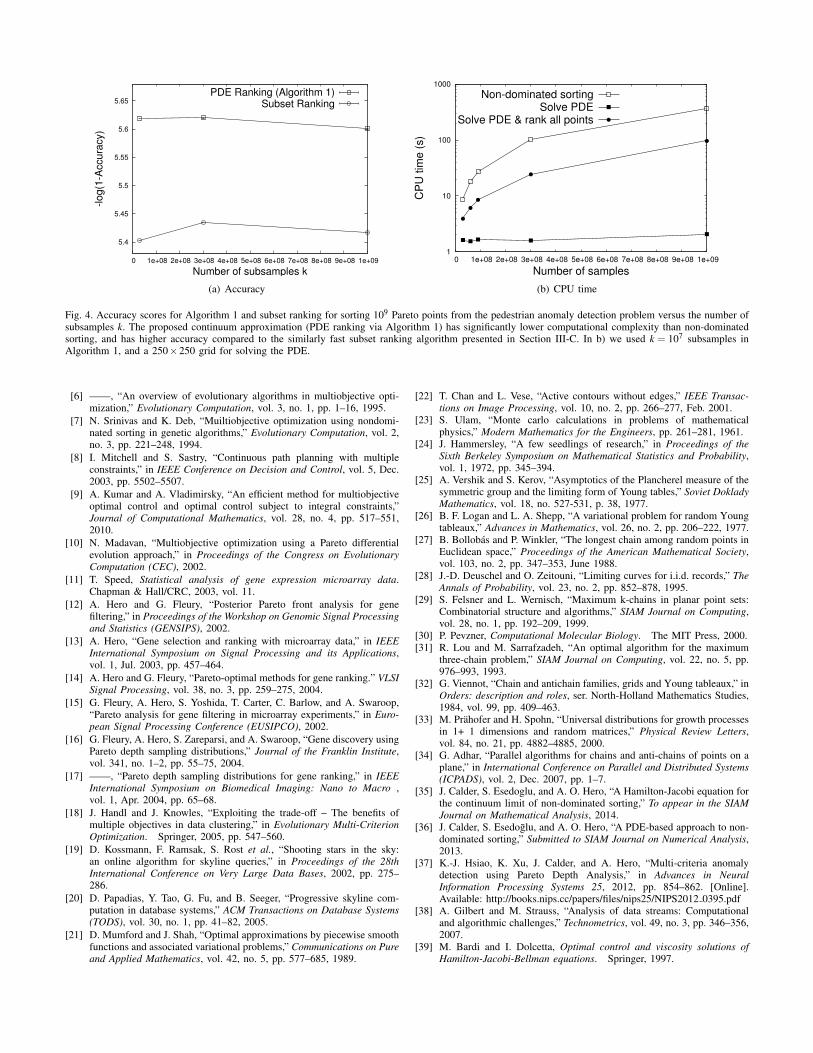
Figure 4 shows the accuracy scores for Algorithm 1 versusthe number of subsamples k, and the CPU time used byAlgorithm 1 and non-dominated sorting. Notice that we plotted− log(1−Accuracy), since the values are very close to one.Due to the memory requirements for non-dominated sorting,we cannot sort datasets significantly larger than than 109

points. In order to have ground truth to compare against,we used only 44722 out of 110035 trajectories, yieldingapproximately 109 Pareto points. Note that a 500× 500 gridwas used for solving the PDE, and we show the CPU timefor steps 1) and 2) (Solve PDE) separate from the time toexecute all of Algorithm 1 to illustrate the sublinearity of thisportion of the algorithm. We compared against the O(n logn)non-dominated sorting algorithm given in [29], [4].

We also compare Algorithm 1 against a naıve algorithmfor fast non-dominated sorting. We call the algorithm subsetranking [36], and the idea is to randomly sample k pointsfrom X1, . . . ,Xn, sort this small subset, and then extrapolate thePareto ranks to the larger dataset X1, . . . ,Xn. Subset ranking isfast—comparable to Algorithm 1—but there is no reason to

expect it to be accurate. In Figure 4, we show the accuracy ofsubset ranking. Although it is not as accurate as Algorithm 1,the strong performance of subset ranking is quite surprising,and there is, to our knowledge, no rigorous justification forthis. We note also that Xi, j1≤i< j≤M are not i.i.d., since theyare elements of a Euclidean dissimilarity matrix, so theseresults are also strong evidence that Theorem 1 holds for somespecial cases of non-i.i.d. random variables.

IV. CONCLUSION

In conclusion, we have presented an overview of our recentwork on a continuum limit for non-dominated sorting [35],[36]. We identified a Hamilton-Jacobi partial differential equa-tion (PDE) for this continuum limit, and showed how tonumerically solve the PDE efficiently. We presented a fastapproximate non-dominated sorting algorithm based on nu-merically solving this PDE, and applied the algorithm toreal-world data from an anomaly detection problem withfavorable results. We expect this work to be useful in othermulti-objective optimization problems as well; in particular, itseems very well-suited for big data problems in the streamingcontext [38].

ACKNOWLEDGMENT

The research described in this paper was partially supportedby ARO grant W911NF-09-1-0310 and NSF grants CCF-1217880 and DMS-0914567.

REFERENCES

[1] M. Ehrgott, Multicriteria Optimization (2. ed.). Springer, 2005.[2] K. Deb, Multi-objective optimization using evolutionary algorithms.

Wiley, Chichester, UK, 2001.[3] K. Deb, A. Pratap, S. Agarwal, and T. Meyarivan, “A fast and elitist

multiobjective genetic algorithm: NSGA-II,” IEEE Transactions onEvolutionary Computation, vol. 6, no. 2, pp. 182–197, 2002.

[4] M. Jensen, “Reducing the run-time complexity of multiobjective EAs:The NSGA-II and other algorithms,” IEEE Transactions on EvolutionaryComputation, vol. 7, no. 5, pp. 503–515, 2003.

[5] C. Fonseca and P. Fleming, “Genetic algorithms for multiobjectiveoptimization : formulation, discussion and generalization,” Proceedingsof the Fifth International Conference on Genetic Algorithms, vol. 1, pp.416–423, Jul. 1993.

5.4

5.45

5.5

5.55

5.6

5.65

0 1e+08 2e+08 3e+08 4e+08 5e+08 6e+08 7e+08 8e+08 9e+08 1e+09

-log(1

-Accu

racy)

Number of subsamples k

PDE Ranking (Algorithm 1)Subset Ranking

(a) Accuracy

1

10

100

1000

0 1e+08 2e+08 3e+08 4e+08 5e+08 6e+08 7e+08 8e+08 9e+08 1e+09

CP

U tim

e (

s)

Number of samples

CPU time (s) vs Number of samples

Non-dominated sortingSolve PDE

Solve PDE & rank all points

(b) CPU time

Fig. 4. Accuracy scores for Algorithm 1 and subset ranking for sorting 109 Pareto points from the pedestrian anomaly detection problem versus the number ofsubsamples k. The proposed continuum approximation (PDE ranking via Algorithm 1) has significantly lower computational complexity than non-dominatedsorting, and has higher accuracy compared to the similarly fast subset ranking algorithm presented in Section III-C. In b) we used k = 107 subsamples inAlgorithm 1, and a 250×250 grid for solving the PDE.

[6] ——, “An overview of evolutionary algorithms in multiobjective opti-mization,” Evolutionary Computation, vol. 3, no. 1, pp. 1–16, 1995.

[7] N. Srinivas and K. Deb, “Muiltiobjective optimization using nondomi-nated sorting in genetic algorithms,” Evolutionary Computation, vol. 2,no. 3, pp. 221–248, 1994.

[8] I. Mitchell and S. Sastry, “Continuous path planning with multipleconstraints,” in IEEE Conference on Decision and Control, vol. 5, Dec.2003, pp. 5502–5507.

[9] A. Kumar and A. Vladimirsky, “An efficient method for multiobjectiveoptimal control and optimal control subject to integral constraints,”Journal of Computational Mathematics, vol. 28, no. 4, pp. 517–551,2010.

[10] N. Madavan, “Multiobjective optimization using a Pareto differentialevolution approach,” in Proceedings of the Congress on EvolutionaryComputation (CEC), 2002.

[11] T. Speed, Statistical analysis of gene expression microarray data.Chapman & Hall/CRC, 2003, vol. 11.

[12] A. Hero and G. Fleury, “Posterior Pareto front analysis for genefiltering,” in Proceedings of the Workshop on Genomic Signal Processingand Statistics (GENSIPS), 2002.

[13] A. Hero, “Gene selection and ranking with microarray data,” in IEEEInternational Symposium on Signal Processing and its Applications,vol. 1, Jul. 2003, pp. 457–464.

[14] A. Hero and G. Fleury, “Pareto-optimal methods for gene ranking.” VLSISignal Processing, vol. 38, no. 3, pp. 259–275, 2004.

[15] G. Fleury, A. Hero, S. Yoshida, T. Carter, C. Barlow, and A. Swaroop,“Pareto analysis for gene filtering in microarray experiments,” in Euro-pean Signal Processing Conference (EUSIPCO), 2002.

[16] G. Fleury, A. Hero, S. Zareparsi, and A. Swaroop, “Gene discovery usingPareto depth sampling distributions,” Journal of the Franklin Institute,vol. 341, no. 1–2, pp. 55–75, 2004.

[17] ——, “Pareto depth sampling distributions for gene ranking,” in IEEEInternational Symposium on Biomedical Imaging: Nano to Macro ,vol. 1, Apr. 2004, pp. 65–68.

[18] J. Handl and J. Knowles, “Exploiting the trade-off – The benefits ofmultiple objectives in data clustering,” in Evolutionary Multi-CriterionOptimization. Springer, 2005, pp. 547–560.

[19] D. Kossmann, F. Ramsak, S. Rost et al., “Shooting stars in the sky:an online algorithm for skyline queries,” in Proceedings of the 28thInternational Conference on Very Large Data Bases, 2002, pp. 275–286.

[20] D. Papadias, Y. Tao, G. Fu, and B. Seeger, “Progressive skyline com-putation in database systems,” ACM Transactions on Database Systems(TODS), vol. 30, no. 1, pp. 41–82, 2005.

[21] D. Mumford and J. Shah, “Optimal approximations by piecewise smoothfunctions and associated variational problems,” Communications on Pureand Applied Mathematics, vol. 42, no. 5, pp. 577–685, 1989.

[22] T. Chan and L. Vese, “Active contours without edges,” IEEE Transac-tions on Image Processing, vol. 10, no. 2, pp. 266–277, Feb. 2001.

[23] S. Ulam, “Monte carlo calculations in problems of mathematicalphysics,” Modern Mathematics for the Engineers, pp. 261–281, 1961.

[24] J. Hammersley, “A few seedlings of research,” in Proceedings of theSixth Berkeley Symposium on Mathematical Statistics and Probability,vol. 1, 1972, pp. 345–394.

[25] A. Vershik and S. Kerov, “Asymptotics of the Plancherel measure of thesymmetric group and the limiting form of Young tables,” Soviet DokladyMathematics, vol. 18, no. 527-531, p. 38, 1977.

[26] B. F. Logan and L. A. Shepp, “A variational problem for random Youngtableaux,” Advances in Mathematics, vol. 26, no. 2, pp. 206–222, 1977.

[27] B. Bollobas and P. Winkler, “The longest chain among random points inEuclidean space,” Proceedings of the American Mathematical Society,vol. 103, no. 2, pp. 347–353, June 1988.

[28] J.-D. Deuschel and O. Zeitouni, “Limiting curves for i.i.d. records,” TheAnnals of Probability, vol. 23, no. 2, pp. 852–878, 1995.

[29] S. Felsner and L. Wernisch, “Maximum k-chains in planar point sets:Combinatorial structure and algorithms,” SIAM Journal on Computing,vol. 28, no. 1, pp. 192–209, 1999.

[30] P. Pevzner, Computational Molecular Biology. The MIT Press, 2000.[31] R. Lou and M. Sarrafzadeh, “An optimal algorithm for the maximum

three-chain problem,” SIAM Journal on Computing, vol. 22, no. 5, pp.976–993, 1993.

[32] G. Viennot, “Chain and antichain families, grids and Young tableaux,” inOrders: description and roles, ser. North-Holland Mathematics Studies,1984, vol. 99, pp. 409–463.

[33] M. Prahofer and H. Spohn, “Universal distributions for growth processesin 1+ 1 dimensions and random matrices,” Physical Review Letters,vol. 84, no. 21, pp. 4882–4885, 2000.

[34] G. Adhar, “Parallel algorithms for chains and anti-chains of points on aplane,” in International Conference on Parallel and Distributed Systems(ICPADS), vol. 2, Dec. 2007, pp. 1–7.

[35] J. Calder, S. Esedoglu, and A. O. Hero, “A Hamilton-Jacobi equation forthe continuum limit of non-dominated sorting,” To appear in the SIAMJournal on Mathematical Analysis, 2014.

[36] J. Calder, S. Esedoglu, and A. O. Hero, “A PDE-based approach to non-dominated sorting,” Submitted to SIAM Journal on Numerical Analysis,2013.

[37] K.-J. Hsiao, K. Xu, J. Calder, and A. Hero, “Multi-criteria anomalydetection using Pareto Depth Analysis,” in Advances in NeuralInformation Processing Systems 25, 2012, pp. 854–862. [Online].Available: http://books.nips.cc/papers/files/nips25/NIPS2012 0395.pdf

[38] A. Gilbert and M. Strauss, “Analysis of data streams: Computationaland algorithmic challenges,” Technometrics, vol. 49, no. 3, pp. 346–356,2007.

[39] M. Bardi and I. Dolcetta, Optimal control and viscosity solutions ofHamilton-Jacobi-Bellman equations. Springer, 1997.

[40] M. Crandall, H. Ishii, and P. Lions, “User’s guide to viscosity solutionsof second order partial differential equations,” Bulletin of the AmericanMathematical Society, vol. 27, no. 1, pp. 1–67, Jul. 1992.

[41] A. Tsybakov, Introduction to nonparametric estimation. Springer, 2009.[42] D. Loftsgaarden and C. Quesenberry, “A nonparametric estimate of a

multivariate density function,” The Annals of Mathematical Statistics,pp. 1049–1051, 1965.

[43] A. P. Korostelev and A. B. Tsybakov, Minimax theory of image recon-struction. Springer-Verlag, New York, 1993.

[44] B. Majecka, “Statistical models of pedestrian behaviour in the forum,”Master’s thesis, School of Informatics, University of Edinburgh, 2009.