A Contribution to HealthCapital Theory TITUS GALAMA

WR-831

January 2011

This paper series made possible by the NIA funded RAND Center for the Study

of Aging (P30AG012815) and the NICHD funded RAND Population Research

Center (R24HD050906).

WORK ING P A P E R

This product is part of the RAND Labor and Population working paper series. RAND working papers are intended to share researchers’ latest findings and to solicit informal peer review. They have been approved for circulation by RAND Labor and Population but have not been formally edited or peer reviewed. Unless otherwise indicated, working papers can be quoted and cited without permission of the author, provided the source is clearly referred to as a working paper. RAND’s publications do not necessarily reflect the opinions of its research clients and sponsors.

is a registered trademark.

A contribution to health capital theory∗

Titus J. Galama†

January 19, 2011

Abstract

I present a theory of the demand for health, health investment and longevity, building

on the human capital framework for health and addressing limitations of existing

models. I predict a negative correlation between health investment and health, that

the health of wealthy and educated individuals declines more slowly and that they

live longer, that current health status is a function of the initial level of health and the

histories of prior health investments made, that health investment rapidly increases

near the end of life and that length of life is finite as a result of limited life-time

resources (the budget constraint). I derive a structural relation between health and

health investment (e.g., medical care) that is suitable for empirical testing.

Keywords: socioeconomic status, education, health, demand for health, health capital, medical

care, life cycle, age, labor, mortality

JEL Codes : D91, I10, I12, J00, J24

∗This research was supported by the National Institute on Aging, under grants R01AG030824, R01AG037398,

P30AG012815 and P01AG022481. I am grateful to Isaac Ehrlich, Michael Grossman, Hans van Kippersluis, Arie

Kapteyn, Arthur van Soest, Eddy van Doorslaer and Erik Meijer for extensive discussions and detailed comments.†RAND Corporation

1

1 Introduction

The demand for health is one of the most central topics in Health Economics. The canonical model

of the demand for health and health investment (e.g., medical care) arises from Grossman (1972a,

1972b, 2000) and theoretical extensions and competing economic models are still relatively few.

In Grossman’s human capital framework individuals demand medical care (e.g., invest time and

consume medical goods and services) for the consumption benefits (health provides utility) as well

as production benefits (healthy individuals have greater earnings) that good health provides. The

model provides a conceptual framework for interpretation of the demand for health and medical

care in relation to an individual’s resource constraints, preferences and consumption needs over

the life cycle. Arguably the model has been one of the most important contributions of Economics

to the study of health behavior. It has provided insight into a variety of phenomena related to

health, medical care, inequality in health, the relationship between health and socioeconomic

status, occupational choice, etc (e.g., Cropper, 1977; Muurinen and Le Grand, 1985; Case and

Deaton, 2005) and has become the standard (textbook) framework for the economics of the derived

demand for medical care.

Yet several authors have identified limitations to the literature spawned by Grossman’s seminal

1972 papers1 (see Grossman, 2000, for a review and rebuttal of some of these limitations). A

standard framework for the demand for health, health investment (e.g., medical care) and longevity

has to meet the significant challenge of providing insight into a variety of complex phenomena.

Ideally it would explain the significant differences observed in the health of socioeconomic status

(SES) groups - often called the “SES-health gradient”. In the United States, a 60-year-old

top-income-quartile male reports to be in similar health as a 20-year-old bottom-income-quartile

male (Case and Deaton 2005) and similar patterns hold for other measures of SES, such as

education and wealth, and other indicators of health, such as disability and mortality (e.g., Cutler

et al. 2010; van Doorslaer et al. 2008). Initially diverging, the disparity in health between low- and

high-SES groups appears to narrow after ages 50-60. Yet, Case and Deaton (2005) have argued

that health production models are unable to explain differences in the health deterioration rate (not

just the level) between socioeconomic groups.

Another stylized fact of the demand for medical care is that healthy individuals do not go to the

doctor much: a strong negative correlation is observed between measures of health and measures

of health investment. However, Wagstaff (1986a) and Zweifel and Breyer (1997) have pointed to

the inability of health production models to predict the observed negative relation between health

and the demand for medical care.

Introspection and casual observation further suggests that healthy individuals are those that

began life healthy and that have invested in health over the life course. Thus one would expect

that health depends on initial conditions (e.g., initial health) and the history of health investments,

prices, wages, medical technology and environmental conditions. Yet, Usher (1975) has pointed

to the lack of “memory” in model solutions. For example the solution for health typically does not

1Throughout this paper I refer to this literature as the health production literature.

2

depend on its initial value or the histories of health investment and biological aging.

Further, Case and Deaton (2005) note that “. . . If the rate of biological deterioration isconstant, which is perhaps implausible but hardly impossible, . . . people will “choose” an infinitelife . . . ”. This suggests that complete health repair is possible, regardless of the speed of the

process (the rate itself does not matter in causing health to decline) and regardless of the budget

constraint, and as a result declines in health status are driven, not by the rate of deterioration of the

health stock, but by the rate of increase of the rate of deterioration (Case and Deaton, 2005). Thus

a necessary condition in health production models is that the biological aging rate increases with

age to ensure that life is finite and health declines and to reproduce the observed rapid increase in

medical care near the end of life. Case and Deaton (2005) argue, however, that a technology that

can effect such complete health repair is implausible.

Last, Ehrlich and Chuma (1990) have pointed out that under the constant returns to scale

(CRTS) health production process assumed in the health production literature, the marginal cost

of investment is constant, and no interior equilibrium for health investment exists. Ehrlich and

Chuma argue that this is a serious limitation that introduces a type of indeterminacy (“bang-bang”)

problem with respect to optimal investment and health maintenance choices. The importance of

this observation appears to have gone relatively unnoticed: contributions to the literature that

followed the publication of Ehrlich and Chuma’s work in 1990 have continued to assume a health

production function with CRTS in health investment.2 This may have been as a consequence of

the following factors: First, Ehrlich and Chuma’s finding that health investment is undetermined

(under the usual assumption of a CRTS health production process) was incidental to their main

contribution of introducing the demand for longevity (or “quantity of life”) and the authors did not

explore the full implications of a DRTS health production process. Second, Ehrlich and Chuma’s

argument is brief and technical.3 This has led Reid (1998) to argue that “. . . the authors [Ehrlichand Chuma] fail to substantiate either claim [bang-bang and indeterminacy] . . . ”, suggesting

there is room for further research into the argument made by Ehrlich and Chuma. Third, there was

the incorrect notion that Ehrlich and Chuma had changed the structure of the model substantially

and that the alleged indeterminacy of health investment did not apply to the original formulation in

discrete time (e.g., Reid, 1998). Last, because of the increased complexity of a health production

model that includes endogenous length of life (demand for longevity) Ehrlich and Chuma (1990)

had to resort to a particular sensitivity analysis, suitable to optimal control problems (Oniki, 1973),

2E.g., Bolin et al. (2001, 2003); Case and Deaton (2005); Erbsland, Ried and Ulrich (2002); Jacobsen (2000); Leu

and Gerfin (1992); Liljas (1998); Nocera and Zweifel (1998); Wagstaff (1986a); Ried (1996, 1998). To the best of

my knowledge the only exception is an unpublished working paper by Dustmann and Windmeijer (2000) who take the

model by Ehrlich and Chuma (1990) as their point of departure. Bolin et al. (2002a, 2002b) assume that the health

investment function is a decreasing function of health. Thus they impose a relationship between health and health

investment to ensure that the level of investment in health decreases with the health stock rather than deriving this result

from first principles.3It involves a reference to a graph with health investment on one axis and the ratio of two Lagrange multipliers on

the other. The authors note that the same results hold in a discrete time setting, using a proof based on the last period

preceeding death (see their footnote 4).

3

in which the directional effect of a parameter change can be investigated. Ehrlich and Chuma’s

(1990) insightful work is therefore limited to generating directional predictions. This suggested

that obtaining insight into the characteristics of a DRTS health production model would require

numerical analysis or the kind of sensitivity analysis performed by Ehrlich and Chuma (1990)

– while it would not substantially change the nature of the theory. For example, it was thought

that introducing DRTS would result in individuals reaching the desired health stock gradually

rather than instantaneously (e.g., Grossman, 2000, p. 364) – perhaps not a sufficiently important

improvement to warrant the increased level of complexity.

What then is needed to address the above mentioned limitations? I argue that the answer

is two-fold: 1) a reinterpretation is needed of the health stock equilibrium condition, one of the

most central relations in the health production literature, as determining the optimal level of health

investment and not the “optimal” level of the health stock, and 2) one needs to assume DRTS in

the health production process as Ehrlich and Chuma (1990) have argued.

In this paper I present a theory of the demand for health, health investment and longevity

based on Grossman (1972a, 1972b) and the extended version of this model by Ehrlich and Chuma

(1990). In particular, this paper explores in detail the implications of a DRTS health production

process. The theory I develop is capable of reproducing the phenomena discussed above and of

addressing the above mentioned five limitations.

This paper contributes to this literature as follows. First, I reduce the complexity of a theory

with a DRTS health production process (as in Ehrlich and Chuma, 1990) by arguing for a different

interpretation of the health stock equilibrium condition, one of the most central relations in the

health production literature: this relation determines the optimal level of health investment (not

the health stock), conditional on the level of the health stock. The health production literature

has thus far not employed the alternative interpretation of the health equilibrium condition and

consistently utilizing it allows me to develop the health production literature further than was

previously possible. This is because the equilibrium condition for the health stock is of a much

simpler form than the condition which is typically utilized to determine the optimal level of health

investment. Many of the subsequent contributions this paper makes follow from the alternative

interpretation advocated here.

Second, I show that the alternative interpretation allows for an intuitive understanding as to

why the assumption of DRTS in the health production function is necessary, or no solution to the

optimization problem exists. Essentially, the CRTS process as utilized in the health production

literature represents a degenerate case. This is no new result (Ehrlich and Chuma, 1990), but this

paper provides more intuitive, less technical and additional arguments as to why health investment

is not determined under the assumption of a CRTS health production process. This is important

because the implications of the indeterminacy are substantial (e.g., Ehrlich and Chuma, 1990), yet

the debate does not appear to have been settled in favor of a DRTS health production process as

illustrated by its lack of use in the health production literature.

Third, the alternative interpretation allows for explorations of a stylized representation of the

first-order condition which enable an intuitive understanding of the optimal solution for health

4

investment. I find that a unique optimal solution for health investment exists (thus addressing

the indeterminacy as Ehrlich and Chuma, 1990, have also shown). Given an optimal level for

health investment, and because in this interpretation the health stock is determined by the dynamic

equation for health, the stock is found to be a function of the histories of past health investments

and past biological aging rates, addressing the criticism of Usher (1975). Further, I find that the

optimal level of health investment decreases with the user cost of health capital and increases with

wealth and with the consumption and production benefit of health. Thus I show that one does not

need to resort to numerical analyses to gain insight into the characteristics of the solution. This

is important because, arguably, the Grossman model has been successful, in part, because of its

ability to guide empirical analyses through the intuition that simple representations provide (e.g.,

Wagstaff, 1986b; Muurinen and Le Grand, 1985).

Fourth, the alternative interpretation allows developing relations for the effects of variations

in SES (wealth, education) and in health on the optimal level of health investment.4 These

relations complement explorations of stylized representations by allowing one to distinguish first-

from second- and third-order effects and to explore the mechanisms (pathways) that combine to

produce the final directional outcome, again, without the need to resort to numerical analyses.

Under plausible assumptions the theory predicts a negative correlation between health and health

investment (in cross-section). This is an important new result that addresses the criticism by

Wagstaff (1986a) and Zweifel and Breyer (1997). Further, greater wealth, higher earnings over

the life cycle and more education and experience are associated with slower health deterioration,

addressing the criticism by Case and Deaton (2005).5

Fifth, empirical tests of the health production literature have thus far been based on structural

and reduced form equations derived under the assumption of a CRTS health production process.

Arguably, health capital theory has not yet been properly tested because these structural and

reduced form relations suffer from the issue of the indeterminacy of health investment (and

essentially represent a degenerate case). Absent an equivalent relation for a DRTS health

production process I once more employ the alternative interpretation to derive a structural relation

between health and health investment (e.g., medical care) that is suitable for empirical testing. The

structural relation contains the CRTS health production process as a special case, thereby allowing

empirical tests to verify or reject this common assumption in the health production literature.

Last, I perform numerical simulations to illustrate the properties of the theory. These

simulations show that the model is capable of reproducing the rapid increase in health investment

near the end of life and that the optimal solution for length of life is finite for a constant biological

aging rate, addressing the criticism by Case and Deaton (2005) that health production models are

characterized by complete health repair. In sum, I find that the theory can address each of the five

limitations discussed above.

4Employing Oniki’s (1973) method as in Ehrlich and Chuma (1990) is somewhat comparable to the analysis

performed here. Unfortunately, due to space limitations, the detailed analysis underlying the directional predictions

by Ehrlich and Chuma (1990) has not been published, but is available on request from the authors.5These results are also obtained by exploring a stylized representation of the first-order condition.

5

The paper is organized as follows. Section 2 presents the model in discrete time and discusses

the characteristics of the first-order conditions. In particular this section offers an alternative

interpretation of the first-order conditions. Section 3 explores the properties of a DRTS health

production process, in several ways, by: a) exploring a stylized representation of the first-order

condition for health investment to gain an intuitive understanding of its properties, b) analyzing

the effect of differences in health and socioeconomic status (wealth and education) on the optimal

level of health investment and consumption, c) developing structural-form relations for empirical

testing of the model and d) presenting numerical simulations of health, health investment, assets

and consumption profiles and length of life. Section 4 summarizes and concludes. The Appendix

provides detailed derivations and mathematical proofs.

2 The demand for health, health investment and longevity

I start with Grossman’s basic formulation (Grossman, 1972a, 1972b, 2000) for the demand for

health and health investment (e.g., medical care) in discrete time (see also Wagstaff, 1986a; Wolfe,

1985; Zweifel and Breyer, 1997; Ehrlich and Chuma, 1990).6 Health is treated as a form of

human capital (health capital) and individuals derive both consumption (health provides utility)

and production benefits (health increases earnings) from it. The demand for medical care is a

derived demand: individuals demand “good health”, not the consumption of medical care.

Using discrete time optimal control (e.g., Sydsaeter, Strom and Berck, 2005) the problem can

be stated as follows. Individuals maximize the life-time utility function

T−1∑t=0

U(Ct,Ht)∏tk=1(1 + βk)

, (1)

where individuals live for T (endogenous) periods, βk is a subjective discount factor and

individuals derive utility U(Ct,Ht) from consumption Ct and from health Ht. Time t is measured

from the time individuals begin employment. Utility increases with consumption ∂Ut/∂Ct > 0

and with health ∂Ut/∂Ht > 0.

The objective function (1) is maximized subject to the dynamic constraints:

Ht+1 = f (It) + (1 − dt)Ht, (2)

At+1 = (1 + δt)At + Y(Ht) − pXtXt − pmt

mt, (3)

the total time budget ΩtΩt = τwt

+ τIt+ τCt

+ s(Ht), (4)

6In line with Grossman (1972a; 1972b) and Ehrlich and Chuma (1990) I do not incorporate uncertainty in the health

production process. This would unnecessarily complicate the optimization problem and require numerical methods,

while it is not needed to explain the stylized facts regarding health behavior discussed in this paper. For a detailed

treatment of uncertainty within the Grossman model the reader is referred to Ehrlich (2000), Liljas (1998), and Ehrlich

and Yin (2005).

6

and initial and end conditions: H0, HT , A0 and AT are given. Individuals live for T periods and die

at the end of period T−1. Length of life T (Grossman, 1972a, 1972b) is determined by a minimum

health level Hmin. If health falls below this level Ht ≤ Hmin an individual dies (HT ≡ Hmin).

Health (equation 2) can be improved through investment in health It and deteriorates at the

biological aging rate dt. The relation between the input, health investment It, and the output, health

improvement f (It), is governed by the health production function f (·). The health production

function f (·) is assumed to obey the law of diminishing marginal returns in health investment. For

simplicity of discussion I use the following simple functional form

f (It) = Iαt , (5)

where 0 < α < 1 (DRTS).7,8

Assets At (equation 3) provide a return δt (the rate of return on capital), increase with income

Y(Ht) and decrease with purchases in the market of consumption goods and services Xt and

medical goods and services mt at prices pXtand pmt

, respectively. Income Y(Ht) is assumed

to be increasing in health Ht as healthy individuals are more productive and earn higher wages

(Currie and Madrian, 1999; Contoyannis and Rice, 2001).

Goods and services Xt purchased in the market and own time inputs τCtare used in the

production of consumption Ct. Similarly medical goods and services mt and own time inputs

τItare used in the production of health investment It. The efficiencies of production are assumed

to be a function of the consumer’s stock of knowledge E (an individual’s human capital exclusive

of health capital [e.g., education]) as the more educated may be more efficient at investing in health

(see, e.g., Grossman 2000):

It = I[mt, τIt; E], (6)

Ct = C[Xt, τCt; E]. (7)

The total time available in any periodΩt (equation 4) is the sum of all possible uses τwt(work),

τIt(health investment), τCt

(consumption) and s(Ht) (sick time; a decreasing function of health).

In this formulation one can interpret τCt, the own-time input into consumption Ct as representing

leisure.9

7For α = 1 we have Grossman’s original formulation of a linear health production process.8Mathematically, equation (5) is equivalent to the assumption made by Ehrlich and Chuma (1990) of a dual

cost-of-investment function with decreasing returns to scale (their equation 5) and a linear health production process

(α = 1 in equation 5 in this paper). Conceptually, however, there is an important distinction. In principle one could

imagine a scenario where the investment function It has constant or even increasing returns to scale in its inputs of

health investment goods / services mt and own time τIt, but where the ultimate health improvement (through the health

production process) has diminishing returns to scale in its inputs mt and τItas assumed in equation (5; this paper).

Arguably, it is not the process of health investment but the process of health production (the ultimate effect on health)

that is expected to exhibit decreasing returns to scale.9Because consumption consists of time inputs and purchases of goods/services in the market one can conceive

leisure as a form of consumption consisting entirely or mostly of time inputs. Leisure, similar to consumption, provides

utility and its cost consists of the price of goods/services utilized and the opportunity cost of time.

7

Income Y(Ht) is taken to be a function of the wage rate wt times the amount of time spent

working τwt,

Y(Ht) = wt

[Ωt − τIt

− τCt− s(Ht)

]. (8)

Thus, we have the following optimal control problem: the objective function (1) is maximized

with respect to the control functions Xt, τCt, mt and τIt

and subject to the constraints (2, 3 and 4).

The Hamiltonian of this problem is:

�t =U(Ct,Ht)∏tk=1(1 + βk)

+ qHt Ht+1 + qA

t At+1, t = 0, . . .T − 1 (9)

where qHt is the adjoint variable associated with the dynamic equation (2) for the state variable

health Ht and qAt is the adjoint variable associated with the dynamic equation (3) for the state

variable assets At.10

The optimal control problem presented so far is formulated for a fixed length of life T (see, e.g.,

Seierstad and Sydsaeter, 1977, 1987; Kirk, 1970; see also section 3.4.1). To allow for differential

mortality one needs to introduce an additional condition to the optimal control problem to optimize

over all possible lengths of life T (Ehrlich and Chuma, 1990). One way to achieve this is by first

solving the optimal control problem conditional on length of life T (i.e., for a fixed exogenous T ),

inserting the optimal solutions for consumption C∗t and health H∗t (denoted by ∗) into the “indirect

utility function”

VT ≡T−1∑t=0

U(C∗t ,H∗t )∏t

k=1(1 + βk), (10)

and maximizing VT with respect to T .11

2.1 First-order conditions

Maximization of (9) with respect to the control functions mt and τItleads to the first-order

condition for health investment It

πIt∏tk=1(1 + δk)

= −t∑

i=1

⎡⎢⎢⎢⎢⎢⎢⎣ ∂U(Ci,Hi)/∂Hi

qA0

∏ij=1(1 + β j)

+∂Y(Hi)/∂Hi∏i

j=1(1 + δ j)

⎤⎥⎥⎥⎥⎥⎥⎦ 1∏tk=i(1 − dk)

+πI0∏t

k=1(1 − dk), (11)

10For a CRTS health production function ( f (It) ∝ It) as employed in the health production literature we have to

explicitly impose that health investment is non negative, It ≥ 0 (see Galama and Kapteyn 2009). This can be done

by introducing an additional multiplier qIt in the Hamiltonian (equation 9) associated with the condition that health

investment is non negative, It ≥ 0. This is not necessary for a DRTS health production function, where diminishing

marginal benefits and choice of suitable functional forms ensure that the optimal solution for health investment It is non

negative.11This is mathematically equivalent to the condition utilized by Ehrlich and Chuma (1990) (in continuous time) that

the Hamiltonian equal zero at the end of life �T = 0 (transversality condition).

8

where πItis the marginal cost of health investment It

πIt≡

pmtI1−αt

α[∂It/∂mt]=

wtI1−αt

α[∂It/∂τIt], (12)

and the Lagrange multiplier qA0

is the shadow price of wealth (see, e.g, Case and Deaton, 2005).

An alternative expression is obtained by using the final period T − 1 as point of reference

πIt∏tk=1(1 + δk)

=

T−1∑i=t+1

⎡⎢⎢⎢⎢⎢⎢⎣ ∂U(Ci,Hi)/∂Hi

qA0

∏ij=1(1 + β j)

+∂Y(Hi)/∂Hi∏i

j=1(1 + δ j)

⎤⎥⎥⎥⎥⎥⎥⎦i−1∏

k=t+1

(1 − dk)

+πIT−1

∏T−1k=t+1(1 − dk)∏T

k=1(1 + δk). (13)

Using either the expression (11) or (13) for the first-order condition for health investment and

taking the difference between period t and t − 1 we obtain the following expression

(1 − dt)πIt= πIt−1

(1 + δt) −⎡⎢⎢⎢⎢⎢⎣∂U(Ct,Ht)/∂Ht

∏tj=1(1 + δ j)

qA0

∏tj=1(1 + β j)

+∂Y(Ht)

∂Ht

⎤⎥⎥⎥⎥⎥⎦ , (14)

or

∂U(Ct,Ht)

∂Ht= qA

0

(σHt− ϕHt

) ∏tj=1(1 + β j)∏tj=1(1 + δ j)

, (15)

where σHtis the user cost of health capital at the margin

σHt≡ πIt

⎡⎢⎢⎢⎢⎢⎣(dt + δt) −ΔπIt

πIt

(1 + δt)

⎤⎥⎥⎥⎥⎥⎦ , (16)

ϕHtis the marginal production benefit of health

ϕHt≡ ∂Y(Ht)

∂Ht, (17)

and ΔπIt≡ πIt

− πIt−1.

Maximization of (9) with respect to the control functions Xt and τCtleads to the first-order

condition for consumption Ct

∂U(Ct,Ht)

∂Ct= qA

0πCt

∏tj=1(1 + β j)∏tj=1(1 + δ j)

, (18)

9

where πCtis the marginal cost of consumption Ct

πCt≡

pXt

∂Ct/∂Xt=

wt

∂Ct/∂τCt

. (19)

The first-order condition (11) (or the alternative forms 13 and 15) determines the optimal

solution for the control function health investment It. The first-order condition (18) determines the

optimal solution for the control function consumption Ct.12 The solutions for the state functions

health Ht and assets At then follow from the dynamic equations (2) and (3). Length of life T is

determined by maximizing the indirect utility function VT (see 10) with respect to T .

2.2 An alternative interpretation of the first-order condition

One of the most central relations in the health production literature is the first-order condition

(15). This relation equates the marginal consumption benefit of health ∂Ut/∂Ht to the user cost

of health capital σHtand the marginal production benefit of health ϕHt

, and is interpreted as an

equilibrium condition for the health stock Ht. It is equivalent to, e.g., equation (11) in Grossman

(2000) and equation (13) in Ehrlich and Chuma (1990).13 An alternative interpretation of relation

(15) is, however, that it determines the optimal level of health investment It. My argument is as

follows.

First, the first-order condition (15) is the result of maximization of the optimal control problem

with respect to investment in health and hence, first and foremost, it determines the optimal level

of health investment It. Optimal control theory distinguishes between control functions and state

functions. Control functions are determined by the first-order conditions and state functions by

the dynamic equations (e.g., Seierstad and Sydsaeter, 1977, 1987; Kirk, 1970). The first-order

condition (15) is thus naturally associated with the control function health investment It and the

state function health Ht is determined by the dynamic equation (2).14

Second, in the health production literature the optimal solution for health investment It is

assumed to be determined by the first-order condition (11) (or the alternative form 13). It is

equivalent to, e.g., equation (9) in Grossman (2000) and equation (8) in Ehrlich and Chuma

12Because the first-order condition for health investment goods / services mt and the first-order condition for own time

inputs τItare identical (see Appendix section A) one can consider a single control function It (health investment) instead

of two control functions mt and τIt. The same is true for consumption Ct. Because of this property, the optimization

problem is reduced to two control functions It and Ct (instead of four) and two state functions Ht and At.13Notational differences with respect to Grossman (2000) are: qA

0→ λ, πIt

→ πt, ∂Ut/∂Ht → [∂U/∂ht][∂ht/∂Ht] =

UhtGt (where ht is healthy time, a function of health Ht), ϕHt→ WtGt, δt → r, dt → δt, βt → 0, and T → n.

Notational differences with respect to Ehrlich and Chuma (1990), apart from using discrete rather than continuous

time, are: qA0→ λA(0), πIt

→ g(t), ∂Ut/∂Ht → [∂U(t)/∂h(t)][∂h(t)/∂H(t)] = Uh(t)ϕ′(H(t)) (where h(t) is healthy time),

ϕHt→ wϕ

′(H(t)), δt → r, dt → δ(t) and βt → ρ.

14Analogously, the first-order condition (18) is associated with the control variable consumption Ct and the dynamic

equation (3) is associated with the state function assets At.

10

(1990).15 However, it can be shown that the first-order conditions (11) and (15) are mathematically

equivalent

(11)⇔ (15), (20)

proof of which is provided in the Appendix (section B). Thus if equation (11) is the first-order

condition for health investment It (the interpretation in the health production literature) then

equation (15) is too (and vice versa).

From a purely mathematical standpoint one could conceive the condition (15) as determining

the level of the health stock because a direct relation exists between health Ht and health

investment It, namely the dynamic equation (2). Optimizing with respect to health investment

entails optimizing with respect to health. Thus, in principle, one ought to be able to reconcile

both interpretations. However, the health production literature assumes CRTS in the health

production process.16 In section 3.1.2 I show that under this particular assumption the level of

health investment is not determined, i.e. that it represents a special degenerate case. As a result,

both approaches cannot be reconciled in this particular case.

In the remainder of this paper I will use relations (11) and (15) as being equivalent. Both

conditions determine the optimal level of health investment It, conditional on the level of the

health stock Ht.

3 A DRTS health production process

In this section I explore the properties of a health production process in several ways. In section

3.1 I discuss a stylized representation of the first-order condition for health investment to gain an

intuitive understanding of its properties. In particular I contrast the characteristics of the solution

for health investment under a DRTS health production process with that of a CRTS process.

In this section I also provide additional arguments for the claim made by Ehrlich and Chuma

(1990) that DRTS in the health production process are necessary to guarantee the existence of

a solution to the optimization problem.17 In section 3.2 I explore the effect of differences in

health and socioeconomic status (wealth and education) on the optimal level of health investment

15One important difference between the results derived by Grossman (equation 9 in Grossman, 2000) and those

derived here is the absense in Grossman’s derivations of the reference point πI0in equation (11) or the reference point

πIT−1in equation (13). Using optimal control techniques I find these reference points to be required in a discrete time

formulation (see equations 11 and 13). This is also true for a continuous time formulation. To the best of my knowledge

this observation has not been made before. It has important implications for the model’s interpretation as the begin or

end point references allows one to ensure that the solution is consistent with the begin and end conditions for health

and assets: H0, HT , A

0and AT .

16I.e., f (It) = Iαt with α = 1 (equations 2 and 5) and a Cobb-Douglas (CRTS) relation between investment in medical

care It and its inputs own time and goods/services purchased in the market.17Providing further corroboration of their claim is important because the implications are substantial and the debate

does not appear to have been settled in favor of a DRTS health production process as illustrated by its lack of use in the

health production literature.

11

and consumption. In section 3.3 I derive structural form relations for empirical testing of the

model. Last, in section 3.4 I perform numerical simulations of health, health investment, assets

and consumption profiles and length of life.

In the following I assume diminishing marginal utilities of consumption ∂2Ut/∂C2t < 0 and

of health ∂2Ut/∂Ht < 0, and diminishing marginal production benefit of health ∂ϕHt/∂Ht =

∂2Yt/∂H2t < 0. In addition I make the usual assumption of a Cobb-Douglas CRTS relation between

the inputs goods/services purchased in the market and own-time and the outputs investment in

curative care It and consumption Ct. As a result we have πIt∝ I1−α

t and ∂πCt/∂Ct = 0 (see

equations 81 and 84 in Appendix section D).

3.1 Stylized representation

In this section I contrast the properties of a DRTS health production process18 (section 3.1.1) with

those of a CRTS health production process19 (section 3.1.2).

3.1.1 Decreasing returns to scale

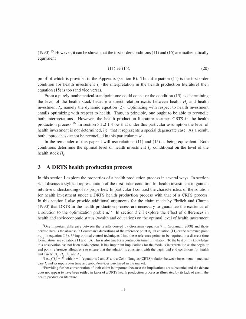
Figure 1 provides a stylized representation of the first-order condition for health investment It(15): it graphs the marginal benefit and marginal cost of health as a function of health investment

It (left-hand side) and as a function of health Ht (right-hand side).20

Consider the left-hand figure first. The optimal level of health investment It is determined by

equating the consumption benefit of health ∂Ut/∂Ht with the cost of maintaining the health stock

qA0

(σHt− ϕHt

) (here and in the remainder of the discussion in this section I ommit for convenience

of notation the term∏t

j=1(1 + β j)[∏t

j=1(1 + δ j)]−1).

Utility is derived from health Ht and consumption Ct but not from health investment It (the

demand for medical care is a derived demand). Further, the evolution of the health stock Ht is

determined by the dynamic equation (2) which can be written (using 5) as

Ht = H0

t−1∏j=0

(1 − d j) +

t−1∑j=0

Iαj

t−1∏i= j+1

(1 − di). (21)

In other words, health Ht is a function of past health investment Is but not of current health

investment It (s < t). Thus the consumption benefit of health ∂Ut/∂Ht is independent of the

level of health investment It: this is shown as the horizontal solid line labeled ∂Ut/∂Ht.

180 < α < 1 and a Cobb-Douglas health investment process It.19α = 1 and a Cobb-Douglas health investment process It.20While in principle one can derive predictions for the level of health investment It from the left-hand figure without

the need to resort to the right-hand figure, it is useful to consider the right-hand figure in order to illustrate the effect of

differences in the health stock Ht on the optimal level of health investment (see section 3.2) and to make comparisons

with the usual interpretation of this relation as determining the “optimal” health stock (rather than optimal investment;

see section 3.1.2).

12

The cost of maintaining the health stock is a function of the shadow price of wealth qA0

,21

the user cost of health capital σHt, the production benefit of health ϕHt

, and an exponential factor

that varies with age t depending on the difference between the time preference rate βt and the

rate of return on capital δt. The marginal cost of health investment πItand hence the user cost of

health capital σHtis increasing in the level of investment in health It (πIt

∝ I1−αt ; see equation

81 in Appendix section D). The marginal production benefit of health ϕHtis not a function of

the level of health investment It. As a result, the cost of maintaining the health stock is upward

sloping in the level of health investment (labeled qA0

(σHt−ϕHt

)). The intersection of the two curves

determines the optimal level of health investment (dotted vertical line labeled It).

tI tI �

t

t

UH��

� �0 t t

AH Hq � ��

t

t

UH��

� �0 t t

AH Hq � ��

tH �tH

Figure 1: Marginal benefit versus marginal cost of health for a DRTS health production process.In labeling the curves I have omitted the term

∏tj=1(1 + β j)[

∏tj=1(1 + δ j)]

−1.

Now consider the right-hand side of Figure 1. The marginal consumption benefit of health

∂Ut/∂Ht is downward sloping (convex) in health (curve labeled ∂Ut/∂Ht) and the cost of

maintaining the health stock qA0

(σHt− ϕHt

) is upward sloping (concave) in health (curve labeled

qA0

(σHt− ϕHt

)) due to the diminishing marginal production benefit of health ϕHt. Since health

is a stock its level is given (dotted vertical line labeled Ht) and provides a constraint: the

two curves have to intersect at this level Ht. It is possible for the two curves to intersect

at Ht through endogenous health investment It. A higher(/lower) level of health investment

It increases(/decreases) (ceteris paribus) the marginal cost of health investment and hence the

user cost of health capital. As a result the cost of maintaining the health stock (curve labeled

qA0

(σHt− ϕHt

)) shifts upward(/downward) while the marginal benefit of health (curve labeled

∂Ut/∂Ht) remains stationary (it is not a function of the level of health investment).

The level of the marginal consumption benefit of health (labeled ∂Ut/∂Ht on the left-hand

21qA0

is decreasing in initial assets and life-time earnings. See, e.g., Wagstaff (1986a).

13

side of Figure 1) for which the health stock is at Ht (draw a horizontal line from the left-hand

to the right-hand side of Figure 1) determines the optimal solution for health investment It. The

optimal level of health investment It decreases with the user cost of health capitalσHtand increases

with wealth (lower qA0

) and with the consumption ∂Ut/∂Ht and production ϕHtbenefit of health.

Further, the optimal level of health investment It is a direct function of the level of health stock

Ht as can be seen from the first-order condition (15) and from its stylized representation in Figure

1 (more on this in the next sections 3.2 and 3.3). Hence, for a DRTS health production process a

unique solution for health investment It exists for every level of the health stock Ht. This addresses

the issue of the indeterminacy of health investment (e.g., Ehrlich and Chuma, 1990).

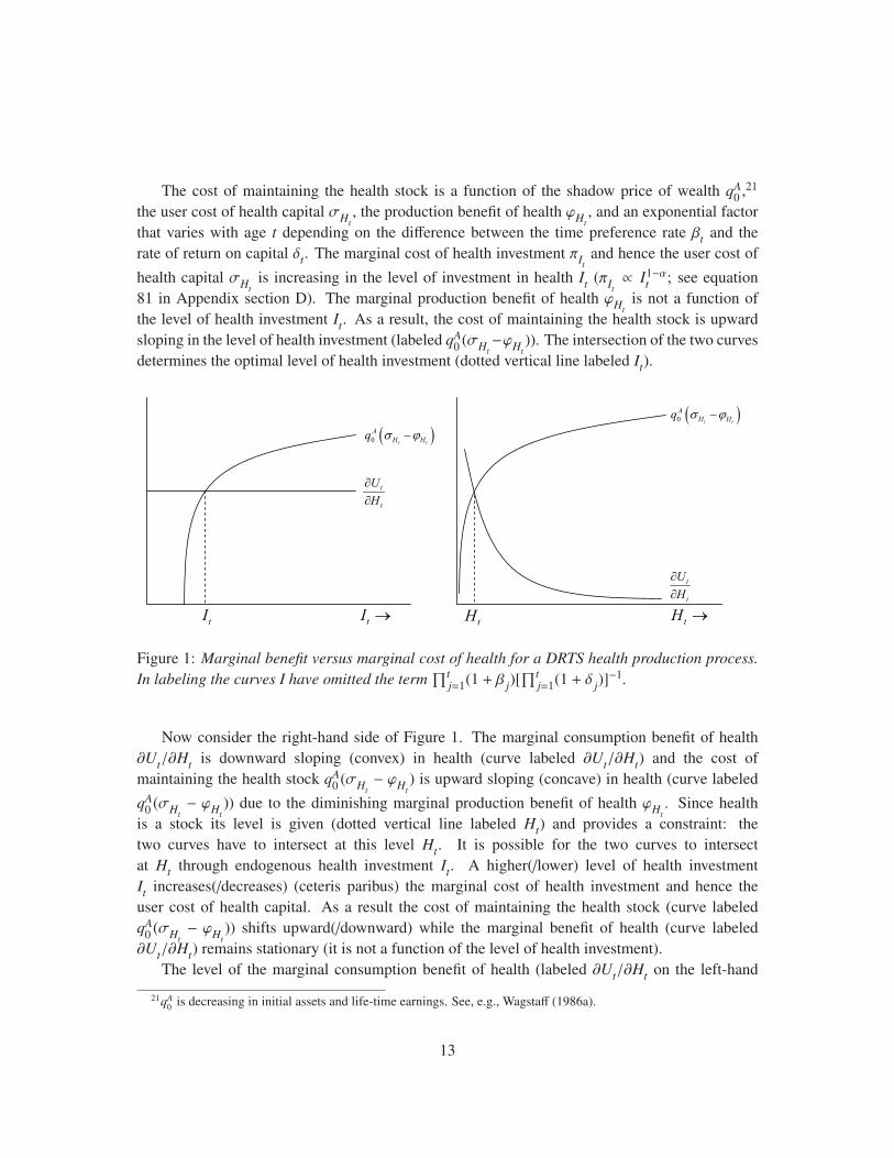
3.1.2 Constant returns to scale

Figure 2 provides a stylized representation of the first-order condition (15) for health investment

for a CRTS health production process, as typically assumed in the health production literature:

it graphs the marginal benefit and marginal cost of health as a function of health investment It(left-hand side) and as a function of the health stock Ht (right-hand side). In the following I follow

the discussion in the previous section 3.1.1 and emphasize the differences with respect to a DRTS

health production process.

� �0 t t

AH Hq � ��

tI �

t

t

UH��

*tH

� �0 t t

AH Hq � ��

tH �

t

t

UH��

Figure 2: Marginal benefit versus marginal cost of health for a CRTS health production process.In labeling the curves I have omitted the term

∏tj=1(1 + β j)[

∏tj=1(1 + δ j)]

−1.

Consider the left-hand side first. Unlike the DRTS process, for a CRTS process the marginal

cost of health investment πIt, and hence the user cost of health capital σHt

, is independent of the

level of health investment It (πIt∝ I1−α

t = constant for α = 1; see equation 81 in Appendix

section D). Thus, not only the marginal utility of health ∂Ut/∂Ht but also the net marginal cost is

independent of the level of health investment It: this is shown as the horizontal solid lines labeled

14

qA0

(σHt− ϕHt

) and ∂Ut/∂Ht.

Because individuals cannot adjust their health instantaneously, the level of the health stock Htat age t is given and provides a constraint for the optimization problem at age t. Generally the

constraint provided by Ht will result in different values for the marginal benefit and marginal cost

of health: this is depicted by the two horizontal lines having distinct levels (they do not overlap).

The intersection of the two solid curves would determine the optimal level of health investment Itbut only in the peculiar case that both lines exactly overlap does such an optimal solution exist.

Thus for most values of the health stock no solution for health investment It exists.

Now consider the right-hand side of Figure 2. The consumption benefit of health ∂Ut/∂Htis downward sloping to represent diminishing marginal utility in health. The cost of maintaining

the health stock qA0

(σHt− ϕHt

) is upward sloping to represent diminishing marginal production

benefits of health ϕHt. As the graph shows, a unique level of health H∗t exists (dashed vertical line)

for which the consumption benefit of health equals the cost of maintaining the health stock. The

health production literature assumes this unique solution H∗t describes the “optimal” health path.

Turning again to the left-hand side of Figure 2, note that for this particular value of the health

stock H∗t the consumption benefit of health ∂Ut/∂Ht and the cost of maintaining the health stock

qA0

(σHt−ϕHt

) overlap (they both lie on the dashed horizontal line). Thus a solution for the level of

investment in health It exists, but any non negative value can be allowed: once more the optimal

level of investment in health It is not determined.

In order to illustrate that this result does not depend on the equivalence of the first-order

conditions (11) and (15) I show next that this result also holds for (11), the relation that is utilized

in the health production literature as determining the optimal level of health investment. The

first-order condition for health investment (11) equates the current marginal monetary cost of

investment in health πIt(left-hand side; LHS) with a function of the current and all past values

of the marginal utility of health ∂Us/∂Hs and the marginal production benefit of health ϕHs(0 ≤ s ≤ t) (right-hand side; RHS). The LHS of (11) is not a function of health investment as

the marginal monetary cost of health investment πItis independent of the level of investment for a

CRTS health production process. The RHS of (11) is also not a function of current investment Itbecause the marginal utility of health ∂Us/∂Hs and the marginal production benefit of health ϕHsare functions of the health stock Hs (0 ≤ s ≤ t) which in turn is a function of past but not current

health investment Is (s < t; see equation 21). Thus the first-order condition for health investment

(11) is not a function of health investment It and the level of health investment is not determined.

Ehrlich and Chuma (1990) have reached the same conclusion on the basis of a technical

argument. From equation (59) or (60) it follows that the marginal monetary cost of health

investment πItis the ratio of two Lagrange multipliers

πIt=

qHt

qAt. (22)

15

The right-hand side of (22) is not a function of health investment It by definition.22,23 For a CRTS

health production proces πItis also not a function of health investment It and hence the level of

health investment is not determined by the first-order conditon for health investment.

3.2 Variation in health and socioeconomic status

In this section I explore the effects of differences in health and socioeconomic status. I employ the

first-order condition (15) to explore the effects of differences in initial assets (section 3.2.1) and in

initial health (section 3.2.2) on the level of health investment It.

3.2.1 Variation in initial assets

Consider two optimal life time trajectories, different only (ceteris paribus) in their initial level of

assets, A0, and, A0 + ΔA0, and the resulting difference in the two optimal life time trajectories

qA0 → qA

0 + ΔqA0,A

Ct → Ct + ΔCt,A

It → It + ΔIt,A

Ht → Ht + ΔHt,A, (23)

where ΔqA0,A, ΔCt,A, ΔIt,A and ΔHt,A denote associated shifts in the shadow price of wealth qA

0

and in the optimal solutions for consumption Ct, health investment It and health Ht at each age

t. A higher capital endowment lowers the shadow price of wealth (i.e., negative ΔqA0,A). This in

turn affects the level of consumption Ct and health investment It over the life cycle. Gradually

differences in health investment It lead to differences in health Ht.

22As Isaac Ehrlich pointed out to me in a private communication, the co-state variables (Lagrangian multipliers)

cannot be a function of the flow of investment because they measure the value of the stocks of health capital and

monetary wealth, which are not affected by the flows of investment in health and earnings, respectively, although they

shift with time in current values. The mathematical proof is part of Pontryagin optimal control theory and the maximum

principle.23Grossman (2000) has questioned the argument by Ehrlich and Chuma (1990) noting (in a discrete time setting) that

the first-order condition for health investment (13) equates the current marginal monetary cost of investment in health

πIt(LHS) with a function of all future values of the marginal utility of health ∂Us/∂Hs and the marginal production

benefit of health ϕHs(t < s ≤ T − 1) (RHS). These in turn are functions of health and health is a function of all

past values of health investment Is (0 ≤ s < t; see equation 21). Thus the RHS of the first-order condition for health

investment (13) is a function of current health investment It (and, in fact, all future and all past values as well) and hence

a solution for health investment It ought to exist. This apparent discrepancy can be reconciled by noting that implicit

in the first-order condition for health investment (13) is the use of the final period t = T − 1 as the point of reference,

while the relation (21) for the health stock uses the initial period t = 0 as the point of reference. Consistently using the

initial period t = 0 as the point of reference, i.e., using the form (11) instead of (13) for the first-order condition for

health investment, one finds that the RHS of (11) is not a function of current investment as the health stock is a function

of past but not current health investment Is (s < t). Likewise, consistently using the final period t = T as the point of

reference, i.e., using the alternative expression Ht = HT /[∏T−1

i=t (1 − di)] −∑T−1

j=t Iαj /[∏ j

i=t(1 − di)] and comparing this

with the first-order condition (13) one finds that the first-order condition is independent of current health investment It.

16

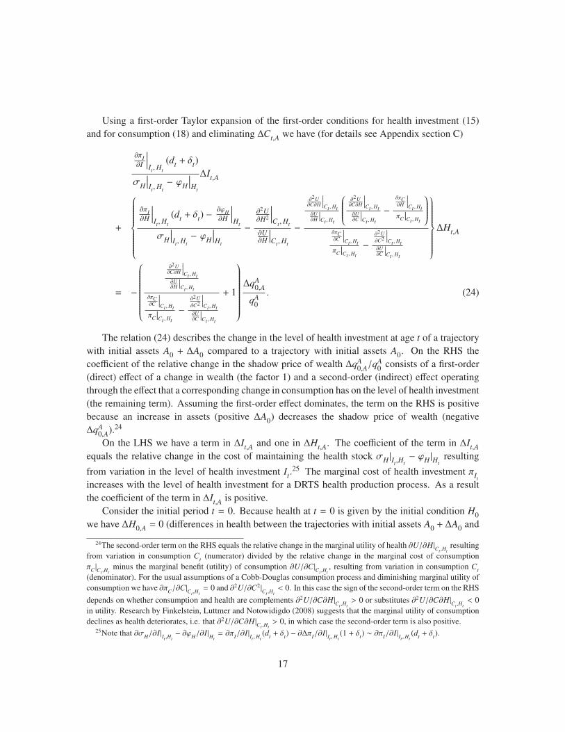
Using a first-order Taylor expansion of the first-order conditions for health investment (15)

and for consumption (18) and eliminating ΔCt,A we have (for details see Appendix section C)

∂πI∂I

∣∣∣∣It ,Ht

(dt + δt)

σH

∣∣∣It ,Ht− ϕH

∣∣∣Ht

ΔIt,A

+

⎧⎪⎪⎪⎪⎪⎪⎪⎪⎪⎨⎪⎪⎪⎪⎪⎪⎪⎪⎪⎩

∂πI∂H

∣∣∣∣It ,Ht

(dt + δt) −∂ϕH∂H

∣∣∣∣Ht

σH

∣∣∣It ,Ht− ϕH

∣∣∣Ht

−∂2U∂H2

∣∣∣∣Ct ,Ht

∂U∂H

∣∣∣Ct ,Ht

−

∂2U∂C∂H

∣∣∣∣Ct ,Ht

∂U∂H

∣∣∣Ct ,Ht

⎛⎜⎜⎜⎜⎜⎜⎝∂2U∂C∂H

∣∣∣∣Ct ,Ht

∂U∂C

∣∣∣Ct ,Ht

−∂πC∂H

∣∣∣∣Ct ,Ht

πC |Ct ,Ht

⎞⎟⎟⎟⎟⎟⎟⎠∂πC∂C

∣∣∣∣Ct ,Ht

πC |Ct ,Ht

−∂2U∂C2

∣∣∣∣Ct ,Ht

∂U∂C

∣∣∣Ct ,Ht

⎫⎪⎪⎪⎪⎪⎪⎪⎪⎪⎬⎪⎪⎪⎪⎪⎪⎪⎪⎪⎭ΔHt,A

= −

⎛⎜⎜⎜⎜⎜⎜⎜⎜⎜⎜⎜⎜⎜⎜⎜⎜⎜⎜⎝

∂2U∂C∂H

∣∣∣∣Ct ,Ht

∂U∂H

∣∣∣Ct ,Ht

∂πC∂C

∣∣∣∣Ct ,Ht

πC |Ct ,Ht

−∂2U∂C2

∣∣∣∣Ct ,Ht

∂U∂C

∣∣∣Ct ,Ht

+ 1

⎞⎟⎟⎟⎟⎟⎟⎟⎟⎟⎟⎟⎟⎟⎟⎟⎟⎟⎟⎠ΔqA

0,A

qA0

. (24)

The relation (24) describes the change in the level of health investment at age t of a trajectory

with initial assets A0 + ΔA0 compared to a trajectory with initial assets A0. On the RHS the

coefficient of the relative change in the shadow price of wealth ΔqA0,A/q

A0

consists of a first-order

(direct) effect of a change in wealth (the factor 1) and a second-order (indirect) effect operating

through the effect that a corresponding change in consumption has on the level of health investment

(the remaining term). Assuming the first-order effect dominates, the term on the RHS is positive

because an increase in assets (positive ΔA0) decreases the shadow price of wealth (negative

ΔqA0,A).24

On the LHS we have a term in ΔIt,A and one in ΔHt,A. The coefficient of the term in ΔIt,Aequals the relative change in the cost of maintaining the health stock σH |It ,Ht

− ϕH |Htresulting

from variation in the level of health investment It.25 The marginal cost of health investment πIt

increases with the level of health investment for a DRTS health production process. As a result

the coefficient of the term in ΔIt,A is positive.

Consider the initial period t = 0. Because health at t = 0 is given by the initial condition H0

we have ΔH0,A = 0 (differences in health between the trajectories with initial assets A0 + ΔA0 and

24The second-order term on the RHS equals the relative change in the marginal utility of health ∂U/∂H|Ct ,Htresulting

from variation in consumption Ct (numerator) divided by the relative change in the marginal cost of consumption

πC |Ct ,Htminus the marginal benefit (utility) of consumption ∂U/∂C|Ct ,Ht

, resulting from variation in consumption Ct(denominator). For the usual assumptions of a Cobb-Douglas consumption process and diminishing marginal utility of

consumption we have ∂πC/∂C|Ct ,Ht= 0 and ∂2U/∂C2|Ct ,Ht

< 0. In this case the sign of the second-order term on the RHS

depends on whether consumption and health are complements ∂2U/∂C∂H|Ct ,Ht> 0 or substitutes ∂2U/∂C∂H|Ct ,Ht

< 0

in utility. Research by Finkelstein, Luttmer and Notowidigdo (2008) suggests that the marginal utility of consumption

declines as health deteriorates, i.e. that ∂2U/∂C∂H|Ct ,Ht> 0, in which case the second-order term is also positive.

25Note that ∂σH/∂I|It ,Ht− ∂ϕH/∂I|Ht

= ∂πI/∂I|It ,Ht(dt + δt) − ∂ΔπI/∂I|It ,Ht

(1 + δt) ∼ ∂πI/∂I|It ,Ht(dt + δt).

17

with A0 occur at later ages). Because ΔH0,A = 0 an increase in assets (which lowers the shadow

price of wealth, i.e., negative ΔqA0,A) increases the level of initial health investment, i.e. positive

ΔI0,A (see equation 24).

A simple graph helps to illustrate this result. Figure 3 shows a stylized representation of

the first-order condition for inital health investment I0 (15) as a function of I0. A higher initial

endowment of capital (positive ΔA0) lowers the shadow price of wealth (negative ΔqA0,A), thus

shifting the net cost of maintaining the health stock downward (curve labeled (q0A + ΔqA

0,A)(σH −ϕH)|I0+ΔI0,A,H0

; first-order effect). A lower shadow price of wealth also increases the initial level

of consumption C0,26 potentially affecting the marginal utility of health (second-order effect). If

consumption and health are complements ∂2U/∂C∂H|Ct ,Ht> 0 in utility, the marginal utility of

health shifts upward (curve labeled ∂U/∂H|C0+ΔC0,A,H0). The net result is a higher level of initial

health investment I0 + ΔI0,A.

A higher initial endowment of capital (positive ΔA0) initially induces individuals to invest

more in health. As a result their health deteriorates slower. This addresses the criticism of Case

and Deaton (2005) that health production models do not predict differences in the effective health

deterioration rate with wealth.

� �0 0

0 ,

AH H I H

q � ��

0I �

0 0, 0,AC C H

UH

��

0 0,AI I 0I

0 0,C H

UH��

� �� �0 0, 0

0 0, ,A

A AA H H I I H

q q � �

�

Figure 3: Differences in initial assets: Marginal consumption ∂U/∂H and marginal productionbenefit ϕH of health versus the user cost of health capital at the margin σH as a function of initialhealth investment I0.

Now consider the next period (t = 1). Because of higher health investment ΔI0,A in the initial

period (t = 0) health will be higher in the next period ΔH1,A > 0 (t = 1). If the level of health

26See equation (77) and note once more that for the usual assumptions of a Cobb-Douglas consumption process and

diminishing marginal utility of consumption we have ∂πC/∂C|Ct ,Ht= 0 and ∂2U/∂C2|Ct ,Ht

< 0. Further, ∂U/∂C|Ct ,Ht> 0

and, for t = 0, ΔH0,A = 0.

18

investment remains higher in subsequent periods, both health trajectories will start to deviate, i.e.

ΔHt,A would grow over time. How would this affect the level of health investment?

The coefficient of ΔHt,A consists of a first-order effect (the first and second terms) and a

second-order effect (the third term). The first term is equal to the relative change in the cost of

maintaining the health stock σH |It ,Ht− ϕH |Ht

resulting from variation in health Ht. The marginal

cost of health investment πI |It ,Htincreases with the wage rate (opportunity cost of investing in

health and not working) which potentially increases with health (healthy individuals are more

productive), i.e. ∂πI/∂H|It ,Ht> 0. Diminishing marginal benefits of health imply ∂ϕH/∂H|Ht

< 0.

Thus the first term is positive. The second term equals the relative change in the marginal

consumption benefit (utility) of health ∂U/∂H|Ct ,Htresulting from variation in health Ht. The

second term is also positive for the usual assumption of diminishing marginal utility of health

∂2U/∂H2|Ct ,Ht< 0. Thus both first-order terms are positive.27 As a result, the difference in the

demand for health investment becomes smaller (smaller ΔIt,A) as the deviation in health between

the trajectories with initial assets A0 + ΔA0 and with A0 grows (growing ΔHt,A; see equation

24). Greater health reduces the demand for health investment (see also the discussions in sections

3.2.2 and 3.3). At some age the difference between the level of health investment could vanish

(ΔIt,A ∼ 0) and the effective health deterioration rate Ht+1 − Ht converge between the trajectory

with initial assets A0+ΔA0 and with A0.28 Despite this convergence, given similar initial endowed

health H0 and an initial period of higher levels of health investment, individuals with greater

endowed wealth remain healthier.

Other indicators of socioeconomic status such as life-time earnings and education behave

qualitatively similar to endowed wealth (initial assets). The exploration of the effect of variations

in these measures on health investment and health is outside the scope of this paper (but see section

3.3 and Galama and van Kippersluis [2010] for a discussion of the role of life-time earnings and

education). The effect of greater earnings over the life cycle on health differs from the effect of

greater endowed wealth in that the “wealth” effect is moderated by the higher opportunity cost of

time. The effect of education on health is similar to that of greater earnings over the life cycle, but

27The third term, describing a second-order effect, contains the same expression as the second-order term in the

coefficient of the relative change in the shadow price of wealth ΔqA0,A/q

A0

(which, following the earlier discussion in

section 3.2.1, is plausible positive) multiplied by the relative change in the marginal utility of health minus the relative

change in the marginal cost of consumption in response to a variation in health: (∂2U/∂C∂H|Ct ,Ht/(∂U/∂H)|Ct ,Ht

−(∂πC/∂H)|Ct ,Ht

/πC |Ct ,Ht. The marginal cost of consumption πC |Ct ,Ht

increases with the wage rate (opportunity cost of

devoting own time to consumption and not working) which potentially increases with health (healthy individuals are

more productive). If consumption and health are strong complements in utility (∂2U/∂C∂H)|Ct ,Ht/(∂U/∂H)|Ct ,Ht

>

(∂πC/∂H|Ct ,Ht)/πC |Ct ,Ht

the third term is positive and results in an elevated level of health investment (compared to a

situation where there is weak complementarity or substitutability in utility) in response to a higher health stock (positive

ΔHt,A).28Note that if at some age the difference in health investment ΔIt,A becomes negative, i.e., an individual with greater

endowed wealth (ΔA0> 0) would spend less on health (ΔIt,A < 0), the health difference in the next period t + 1 is

reduced (smaller ΔHt+1,A), which leads to a less negative or positive difference in the level of health investment ΔIt+1,A,

suggesting a process of gradual convergence in the effective rate of health deterioration Ht+1− Ht (where we have a

relatively constant ΔHt,A and small ΔIt,A).

19

with the additional effect of increasing the efficiency of health investment.

3.2.2 Variation in initial health

Consider two optimal life time trajectories, different only (ceteris paribus) in their initial level of

health, H0, and, H0 + ΔH0, and the resulting difference in initial (t = 0) health investment I0

I0 → I0 + ΔI0,H

C0 → C0 + ΔC0,H

qA0 → qA

0 + ΔqA0,H , (25)

where ΔI0,H , ΔC0,H and ΔqA0,H denote associated shifts in the optimal solution for initial health

investment I0, initial consumption C0 and in the shadow price of wealth qA0

.

Using a first-order Taylor expansion of the first-order conditions for health investment (15)

and for consumption (18), eliminating ΔC0,H , and (in order to simplify the discussion) omitting

second-order effects, we have

∂πI∂I

∣∣∣∣I0,H0

(d0 + δ0)

σH

∣∣∣I0,H0

− ϕH

∣∣∣H0

ΔI0,H

= −

⎧⎪⎪⎪⎪⎪⎨⎪⎪⎪⎪⎪⎩∂πI∂H

∣∣∣∣I0,H0

(d0 + δ0) − ∂ϕH∂H

∣∣∣∣H0

σH

∣∣∣I0,H0

− ϕH

∣∣∣H0

−∂2U∂H2

∣∣∣∣C0,H0

∂U∂H

∣∣∣C0,H0

⎫⎪⎪⎪⎪⎪⎬⎪⎪⎪⎪⎪⎭ΔH0, (26)

(this relation can be obtained by considering 24 for t = 0 and labeling the variations with Hinstead of A).29 The relation (26) describes the change in the initial level of health investment I0

of a trajectory with initial health H0 + ΔH0 compared to a trajectory with initial health H0. Under

the usual assumptions the first-order relation between health and health investment is negative.30

A simple graph helps to illustrate this result. Figure 4 shows a stylized representation of

the first-order condition for the inital level of health investment I0 (15) as a function of I0.

A higher initial endowment of health (positive ΔH0) lowers the marginal production benefit

of health ϕHtthus shifting the net cost of maintaining the health stock upward (curve labeled

29A higher level of initial health (positive ΔH0) enables a higher level of earnings (the production benefit of health),

thereby raising life-time earnings and lowering the shadow price of wealth (negative ΔqA0,H). A higher level of health

would thus increase the level of health investment through its effect on wealth. This wealth effect is however a second

order-effect in the sense that it operates through the effect of health on wealth, and therefore omitted from (26).30The marginal cost of health investment increases with health investment for a DRTS health production process

(i.e., (∂πI/∂I)|I0 ,H0> 0) and with the wage rate (opportunity cost of investing in health and not working) which

potentially increases with health (healthy individuals are more productive; i.e., (∂πI/∂H)|I0 ,H0> 0). Diminishing

marginal production benefit of health implies (∂ϕH/∂H)|H0< 0 and diminishing marginal consumption benefit (utility)

of health implies ∂2U/∂H2|C0 ,H0< 0.

20

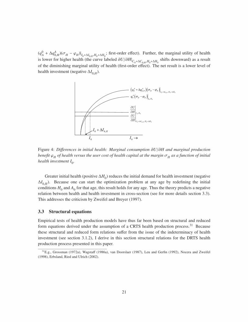
(q0A + ΔqA

0,H)(σH − ϕH)|I0+ΔI0,H ,H0+ΔH0; first-order effect). Further, the marginal utility of health

is lower for higher health (the curve labeled ∂U/∂H|C0+ΔC0,H ,H0+ΔH0shifts downward) as a result

of the diminishing marginal utility of health (first-order effect). The net result is a lower level of

health investment (negative ΔI0,H).

0I 0I �

0 0, 0 0,HC C H H

UH

��

0 0,C H

UH��

0 0,HI I

� �0 0

0 ,

AH H I H

q � ��

� �� �0 0, 0 0

0 0, ,H

A AH H H I I H H

q q � �

�

Figure 4: Differences in initial health: Marginal consumption ∂U/∂H and marginal productionbenefit ϕH of health versus the user cost of health capital at the margin σH as a function of initialhealth investment I0.

Greater initial health (positive ΔH0) reduces the initial demand for health investment (negative

ΔI0,H). Because one can start the optimization problem at any age by redefining the initial

conditions H0 and A0 for that age, this result holds for any age. Thus the theory predicts a negative

relation between health and health investment in cross-section (see for more details section 3.3).

This addresses the criticism by Zweifel and Breyer (1997).

3.3 Structural equations

Empirical tests of health production models have thus far been based on structural and reduced

form equations derived under the assumption of a CRTS health production process.31 Because

these structural and reduced form relations suffer from the issue of the indeterminacy of health

investment (see section 3.1.2), I derive in this section structural relations for the DRTS health

production process presented in this paper.

31E.g., Grossman (1972a), Wagstaff (1986a), van Doorslaer (1987), Leu and Gerfin (1992), Nocera and Zweifel

(1998), Erbsland, Ried and Ulrich (2002).

21

3.3.1 Simple functional forms

In order to obtain expressions suitable for empirical testing we have to assume functional forms

for model functions and parameters that cannot be observed directly, such as the health investment

production process It and the biological aging rate dt.

I specify the following constant relative risk aversion (CRRA) utility function:

U(Ct,Ht) =1

1 − ρ(Cζt H1−ζ

t

)1−ρ, (27)

where ζ (0 ≤ ζ ≤ 1) is the relative “share” of consumption versus health and ρ (ρ > 0) the

coefficient of relative risk aversion. This functional form can account for the observation that

the marginal utility of consumption declines as health deteriorates (e.g., Finkelstein, Luttmer

and Notowidigdo, 2008) which would rule out strongly separable functional forms for the utility

function, where the marginal utility of consumption is independent of health.

I make the usual assumption that sick time is a power law in health

st = Ω

(Ht

Hmin

)−γ, (28)

where γ > 0 so that sick time decreases with health. This choice of functional form has the

properties limHt→∞ st = 0 and limHt↓Hminst = Ω, where Ω is the total time budget as in (4).

Using equation (8) we have:

ϕHt= wtγΩHγ

minH−(1+γ)

t ,

≡ wtΩ∗H−(1+γ)

t . (29)

Investment in medical care It is assumed to be produced by combining own time and

goods/services purchased in the market according to a Cobb-Douglas CRTS production function

(Grossman, 1972a, 1972b, 2000)

It = μItm1−kI

t τkIIt, (30)

where μItis an efficiency factor and 1− kI and kI are the elasticities of investment in health It with

respect to goods and services mt purchased in the market (e.g., medical care) and with respect to

own-time τIt, respectively.

Analagously, consumption Ct is assumed to be produced by combining own time and

goods/services purchased in the market according to a Cobb-Douglas CRTS production function

Ct = μCtX

1−kCt τ

kCCt, (31)

where μCtis an efficiency factor and 1 − kC and kC are the elasticities of consumption Ct with

respect to goods and services Xt purchased in the market and with respect to own-time τCt,

respectively.

22

Following Grossman (1972a, 1972b, 2000) I assume that the more educated are more efficient

consumers and producers of health investment (based on the interpretation of education as a

productivity factor in own time inputs and in identifying and seeking effective care)

μIt= μI0

eρI E , (32)

where E is the level of education (e.g., years of schooling) and ρI is a constant.

Further, following Galama and van Kippersluis (2010) I assume a Mincer-type wage equation

in which the more educated and more experienced earn higher wages (Mincer 1974)

wt = wEeρwE+βx xt−βx2 x2t , (33)

where education E is expressed in years of schooling, xt is years of working experience, and ρw,

βx and βx2 are constants, assumed to be positive.

Lastly, following Wagstaff (1986a) and Cropper (1981) I assume the biological aging rate dtto be of the form

dt = d•eβt t+βξξt , (34)

where d• ≡ d0e−βξξ0 and ξt is a vector of environmental variables (e.g., working and living

conditions, hazardous environment, etc) that affect the biological aging rate. The vector ξtmay include other exogenous variables that affect the biological aging rate, such as education

(Muurinen, 1982).

3.3.2 Structural relation between health and medical care

A structural relation for the demand for medical goods and services mt can be obtained from

the first-order conditions for health investment (15) and for consumption (18) and the functional

relations defined in the previous section 3.3.1 (see section D in the Appendix for details)

b1itm

1−αit − (1 − α)m1−α

it mit = b2itH−1/χit + b3

itH−(1+γ)it , (35)

where I have defined the following functions

b1it ≡

[d•eβt ti+βξξit + δ − (1 − αkI) pmit

− αkIwit

], (36)

b2it ≡ b2

∗(qA

0i

)−1/ρχeαρI Ei p−(1−αkI )

mitw−[kC(1/ρχ−1)+αkI ]

it p−(1−kC)(1/ρχ−1)

Xit

(1 + βi

1 + δ

)−ti/ρχ

(37)

b3it ≡ b3

∗eαρI Ei p−(1−αkI )

mitw1−αkI

it , (38)

23

and the following constants

b2∗ ≡

[(1 − ζ)Λ]1/χ αkαkI

I (1 − kI)1−αkIμαI0

[k

kCC (1 − kC)1−kC μCt

]1/ρχ−1

, (39)

b3∗ ≡ αkαkI

I (1 − kI)1−αkIμαI0

Ω∗, (40)

Λ ≡ ζ1−ρρ

(ζ

1 − ζ)1−χ, (41)

χ ≡ 1 + ρζ − ζρ

, (42)

where the subscript i indexes the ith individual, and where the notation ft is used to denote the

relative change ft ≡ 1− ft−1

ftin a function ft. Further, I have assumed small relative changes (much

smaller than one) in the price of medical care pmit, wages wit and the efficiency of the health

investment process μIitand, for simplicity, assumed a constant discount factor βt = β and constant

rate of return to capital δt = δ.

A similar expression for own-time inputs τIitcan be obtained using (83). Further, one can

substitute the expression (33) for the wage rate wit to obtain an expression in terms of years of

schooling Ei and years of experience xit.

3.3.3 Pure investment and pure consumption models

Analytical solutions to the Grossman model are usually based on two sub-models (1) the

“pure investment” model in which the restriction ∂Ut/∂Ht = 0 is imposed and (2) the “pure

consumption” model in which the restriction ∂Yt/∂Ht = 0 is imposed. In this section I explore

the characteristics of these two sub models for the following reasons. First, the two sub models

represent two essential characteristics of health: health as a means to produce (investment) and

health as a means to provide utility (consumption) and exploring them separately provides insight

into these two distinct properties of health. Second, these restrictions allow one to obtain linearized

structural expressions. Last, the two sub-models are widely used in the health production literature

and exploring them allows for comparisons with previous research.

In the pure investment model health does not provide utility and hence ζ = 1 (see equation 27)

and b2it = 0, whereas in the pure consumption model health does not provide a production benefit

and hence ϕHit= 0 and b3

it = 0. We can obtain a structural linear relation for the demand for health

investment goods / services mit in the pure investment and pure consumption models as follows.

24

Pure investment For small mit and b2it = 0 we have (see equation 35)

(1 − α) ln mit ∼ ln b3it − ln b1

it − (1 + γ) ln Hit,

= ln b3∗ − (1 + γ) ln Hit + αρIEi − (1 − αkI) ln pmit

+ (1 − αkI) ln wit

− ln d• − βitt − βξξit − ln

⎧⎪⎪⎨⎪⎪⎩1 +

⎡⎢⎢⎢⎢⎢⎣δ − (1 − αkI) pmit− αkIwit

d•eβt ti+βξξit

⎤⎥⎥⎥⎥⎥⎦⎫⎪⎪⎬⎪⎪⎭ . (43)

Pure consumption For small mit and b3it = 0 we have (see equation 35)

(1 − α) ln mit ∼ ln b2it − ln b1

it −1

χln Hit,

= ln b2∗ −

1

χln Hit −

1

ρχln qA

0i + αρIEi − (1 − αkI) ln pmit

−[kC (1/ρχ − 1) + αkI

]ln wit − (1 − kC) (1/ρχ − 1) ln pXit

− ln d• − βtti − βξξit

− 1

ρχ

[ln(1 + βi) − ln(1 + δ)

]ti − ln

⎧⎪⎪⎨⎪⎪⎩1 +

⎡⎢⎢⎢⎢⎢⎣δ − (1 − αkI) pmit− αkIwit

d•eβt ti+βξξit

⎤⎥⎥⎥⎥⎥⎦⎫⎪⎪⎬⎪⎪⎭ . (44)

It is customary to assume that the term ln d• in equations (43) and (44) is an error term with

zero mean and constant variance ξ1(t) ≡ − ln d• (as in Wagstaff, 1986a, and Grossman, 1972a,

1972b, 2000) and that the term ln[1+ δt/dt − πIt/dt] (the last term in equations 43 and 44) is small

or constant (see, e.g., Grossman, 1972a, 2000),32 or that it is time dependent ln[1+δt/dt−πIt/dt] ∝ t

(e.g., Wagstaff, 1986a).

3.3.4 Reduced form relations

The solution for the health stock Ht follows from the dynamic equation (2) and using expressions

(32) and (82)

Ht = H0

t−1∏j=0

(1 − d j) +

(1 − kI

kI

)−αkI

μαI0eαρI E

t−1∑j=0

pαkIm j

w−αkIj mαj

t−1∏k= j+1

(1 − dk), (45)

where I have suppressed the index i for the individual.

The health stock Ht is a function of past levels of consumption of medical goods / services

m j ( j ≤ t − 1) and past biological aging rates d j ( j ≤ t − 1). In principle one can obtain reduced

32This would require that the rate of return to capital δt and changes in the wage rate wt and the price pmtand

efficiency μItof health investment goods/services in producing health investment are much smaller than the health

deterioration rate dt or that such changes follow the same pattern as changes in dt (so that the term is approximately

constant).

25

form expressions for the health stock Ht33 and for the demand for medical goods / services mt.

34

This excercise, however, results in complex expressions with arguably limited value for empirical

analyses. The reduced form solutions for the health stock Ht and the demand for medical goods

/ services mt are functions of the initial health stock H0, wealth qA0

(endowed assets and life-time

earnings) and the history of past prices of medical care pms, past prices of consumption goods /

services pXs, past wage rates ws, past biological aging rates ds and past rates of return to capital δs

(s < t). In addition, the demand for medical goods / services is also a function of the current price

of medical care pmt, the current price of consumption goods / services pXt

, the current wage rate

wt, the current biological aging rate dt and the current rate of return to capital δt (the health stock

does not depend on current values).

3.3.5 Discussion

The structural form (35) of the first order condition for health investment describes a direct

relationship between the demand for health investment goods / services mt (e.g., medical care), the

relative change in the demand for health investment goods / services mt and the health stock Ht.

For slow changes in the demand for health investment goods / services with time (small mt), the

demand for health investment goods / services mt falls with the level of health Ht. This is further

reflected in the elasticity of health investment goods / services with respect to health Ht, which,

for small mt, is negative (and a function of the health stock Ht)

σmt ,Ht=∂mt

∂Ht

Ht

mt= − 1

1 − α

⎡⎢⎢⎢⎢⎢⎢⎢⎣1χb2

t H−1/χt + (1 + γ)b3

t H−(1+γ)t

b2t H−1/χ

t + b3t H−(1+γ)

t

⎤⎥⎥⎥⎥⎥⎥⎥⎦ , (46)

where I have suppressed the index i for the individual. Similarly, the elasticity of health investment

goods / services mt with respect to health Ht (see equation 46) for the pure investment model

σPImt ,Ht= −1 + γ

1 − α, (47)

and the pure consumption model

σPCmt ,Ht= − 1

χ(1 − α), (48)

are negative, where the labels PI and PC refer to the pure investment and pure consumption model,

respectively. In other words, I find that the less healthy demand more and the healthy demand less

33Substitute the solutions for past consumption of medical goods / services mj ( j ≤ t − 1) obtained from (35) in

(45) and recursively substitute the expression for the health stock (45) for past values of the health stock to obtain an

expression for the health stock from which past levels of the health stock Hj ( j ≤ t − 1) and past values of consumption

of medical goods / services mj ( j ≤ t − 1) are removed (with the exception of initial health H0).

34Use (35) and recursively substitute the expression for the health stock (45) to obtain an expression from which past

consumption of medical goods / services mj ( j ≤ t − 1) and past levels of the health stock Hj ( j ≤ t − 1) are removed

(again with the exception of initial health H0).

26

medical goods / services. This prediction from the theoretical model is in line with what has been

observed in numerous empirical studies and addresses the criticism by Zweifel and Breyer (1997).

Assuming that both medical goods / services mt and time input τItincrease health investment

suggests 0 ≤ kI ≤ 1 (see equation 30), and if education E increases the efficiency of medical care

then ρI > 0 (see equation 32). Similarly we have 0 ≤ kC ≤ 1 (see equation 31).

For these assumptions and small changes mt, the demand for health investment goods/services

mt (see relations 35 and 36) decreases with the biological aging rate dt (and hence with

environmental factors that are detrimental to health ξt), the rate of return to capital δt (an

opportunity cost – individuals can invest in health or in the stock market) and increases with

price increases pmtand wage increases wt (it is better to invest in health now when prices pmt

and the opportunity cost of time wt are higher in the future). In addition, due to the consumptionaspect of health (health provides utility) the demand for health investment goods/services mt (see

relations 35 and 37 or 44) increases with wealth qA0

−1(the shadow price of wealth is a decreasing

function of wealth and life-time earnings),35 education E (through assumed greater efficiency of

health investment with the level of education) and decreases with the price of health investment

goods/services pmt. For ρχ < 1 the demand for health investment goods/services mt decreases

with the price of consumption goods/services pXt(for ρχ > 1 it increases) and with the wage rate

wt (opportunity cost of time) (for ρχ > 1 the effect of the wage rate wt is ambiguous)). And, due

to the production aspect of health (health increases earnings) the demand for health investment

goods/services mt (see relations 35 and 38 or 43) increases with education E (through assumed

greater efficiency of health investment with the level of education) and the wage rate wt (a higher

wage rate increases the marginal production benefit of health, and this outweighs the opportunity

cost of time associated with health investment) and decreases with the price of health investment

goods/services pmt.

The above discussion masks important effects of earnings and education. In our model of

perfect certainty an evolutionary wage change (along an individual’s wage profile) does not affect

the shadow price of wealth qA0

as the change is fully anticipated by the individual. Thus comparing

panel data for a single individual may reveal a higher wage rate wt to be associated with a lower

demand for medical goods / services mt due to a higher opportunity cost of time. However,

comparing across individuals, those who currently have a higher wage rate will in most cases

also have higher life-time earnings and thus a lower shadow price of wealth qA0

. This wealth effect

increases the demand for medical goods / services and competes with the opportunity cost of time

effect. Similarly, to account for the effect of education it is important not only to consider the

possible effect of a higher efficiency of health investment (the parameter ρI), as in the structural

35In principle, an expression for the shadow price of wealth qA0

can be obtained by using the life-time budget

constraint (which follows from integrating the dynamic equation 3), substituting the solutions for consumption

goods/services Xt, health Ht, and health investment goods/services mt and solving for qA0

(see, for example, Galama

et al. 2008). In practice, the shadow price of wealth qA0

cannot be solved analytically: it is a very complicated function

of the shadow price of health qHt, wealth (assets), education E and earnings, wages wt, prices pmt

, pXt, and health

deterioration rates (terms d•, βt and βξ) over the life cycle.

27

relations (35), (43) and (44), but also the effect that education has on earnings (opportunity cost

of time effect; see equation 33) and in turn on wealth (wealth effect). Plausibly, the wealth

effect dominates the opportunity cost effect. For example, Dustmann and Windmeijer (2000)

and Contoyannis et al. (2004) find a positive effect on health from a permanent wage increase and

a negative effect from a transitory wage increase. We expect then that the effect of education and

earnings is to increase the demand for health investment goods / services through a wealth effect

that may dominate the opportunity cost of time effect associated with higher earnings.36

Thus, in testing the theory it will be important to account for wealth. This can be done by

employing measures of wealth (endowed assets, life-time earnings) as proxies for the shadow price

of wealth qA0

or, following Wagstaff (1986a), by utilizing an approximation for qA0

(his equations

15 and 16).

3.4 Numerical simulations

In this section I present simulations of the model with a DRTS health production process and a

simple step process. I first discuss the step process for fixed length of life (section 3.4.1). I then

illustrate the properties of the model with numerical simulations accounting for endogenous length

of life (section 3.4.2).

3.4.1 Step process and fixed length of life

We start with the initial condition for health H0. Initial consumption C0 then follows from the

first-order condition for consumption (18), which, for the assumed functional forms in section

3.3.1, can be written as

Ct =

⎡⎢⎢⎢⎢⎢⎣qA0

ζπCt

∏tj=1(1 + β j)∏tj=1(1 + δ j)

⎤⎥⎥⎥⎥⎥⎦−1/ρχ

Hχ−1χ

t , (49)

where πCtis given by (19). Initial consumption C0 is a function of initial health H0, the price of

goods and services pX0, the wage rate w0 (the opportunity cost of not working) and the shadow

price of wealth qA0

. Next, the initial level of health investment I0 follows from the initial marginal

cost of curative care πI0(see expression 12) which is a function of the Lagrange multiplier qH

0and

the shadow price of wealth qA0

(πI0= qA

0/qH

0; see equations 59 and 60). The initial level of health

investment I0 is (through the initial marginal cost of curative care πI0) a function of the price of

goods and services pm0, the wage rate w0, education E, and the multipliers qA

0and qH

0. Thus, given

36Further, one may be tempted to conclude that individuals invest less in health care during middle and old age

because of the high opportunity cost of time associated with high earnings at these ages (see equation 33). However,

as health deteriorates with age the demand for curative care increases (see sections 3.2 and 3.3). If the latter effect

dominates, the model is capable of reproducing the observation that young individuals invest little, the middle-aged

invest more and the elderly invest most in curative care.

28

exogenous education, prices and wage rates, the initial level of health investment I0 and the initial

level of consumption C0 are functions of the endogenous Lagrange multipliers qA0

and qH0

.

Health in the next period H1 is determined by the dynamic equation (2). Assets in the next

period A1 follow from the initial condition for assets A0 and the dynamic equation for assets (3).

For the assumed functional forms in section 3.3.1 we have

At+1 = (1 + δt)At + wt

[Ω − τ∗It

It − τ∗CtCt − st

]− pXt

X∗t Ct − pmtm∗t It, (50)

where st, m∗t , τ∗It, X∗t , τ∗Ct

are defined in (28), (82), (83), (85) and (86).

Consumption C1 follows from the first-order condition for consumption (49), health

investment I1 follows from the first-order condition for health investment (11), (13), (14) or (15),

which for the assumed functional forms in section 3.3.1 can be expressed as

πIt=

1

1 − dt

⎡⎢⎢⎢⎢⎣πIt−1(1 + δt) −

1 − ζqA

0

C1−ρχt Hρ(χ−1)−1

t − wtΩ∗H−(1+γ)t

⎤⎥⎥⎥⎥⎦ . (51)

Health H2 and assets A2 in the next period are determined by the dynamic equations (2) and

(50) and so on. The solutions for consumption Ct, health Ht and health investment It for every

period t are functions of the two Lagrange multipliers qA0

and qH0

. In the final period, the two end

conditions for the final level of health HT = Hmin and the final level of assets AT determine the

Lagrange multipliers qA0

and qH0

.37

Some have argued that length of life is determined in an iterative process by the condition that

health at the end of life HT equal the minimum health stock Hmin (e.g., Grossman, 1998; Reid,

1998). These results are however based on a CRTS health production process and are the result

of the indeterminacy of health investment. The results do not hold for a DRTS health production

process as advocated here. This can be seen as follows. As the preceding discussion shows, the

end conditions HT = Hmin and AT are met for fixed length of life T because the solutions for

assets, consumption, health and health investment (and having used the initial conditions H0 and

A0) are functions of the Lagrange multipliers qA0

and qH0

. Applying the end conditions AT and

HT determines the Lagrange multipliers qA0

and qH0

for fixed T . Thus, in the health production

literature, as pointed out by Ehrlich and Chuma (1990), length of life T is exogenous (fixed) in the

absence of the required terminal (transversality) condition.

3.4.2 Simulations with endogenous mortality

In this section I simulate the model for a particular set of parameter values. The purpose of this

exercise is to illustrate some properties of the model. Other parameter choices are possible and

a full exploration of the model’s properties would require exploring a wide range of parameter

values. Ultimately one would like to estimate the model with panel data to test its ability to

describe human behavior. This is beyond the scope of this paper.

37Alternatively one could start with the final period t = T −1 and use recursive back substitution. Reaching the initial

period, the two initial conditions for health H0

and assets A0

determine the Lagrange multipliers qA0

and qHT−1

.

29

20 30 40 50 60 70 80t

20

40

60

80

100H�t�

30 40 50 60 70 80t

�100

100

200

300

A�t�

20 30 40 50 60 70 80t

0.02

0.04

0.06

0.08

0.10I�t�

20 30 40 50 60 70 80t

20

40

60

80

100

120

140

C�t�

30 40 50 60 70 80t

0.2

0.4

0.6

0.8

1.0h�t�

30 40 50 60 70 80t

�10

10

20

30

40

50Y�t�

Figure 5: Health (H(t); top-left panel), assets (A(t); $ thousands; top-right panel), health

investment (I(t); center-left panel), consumption (C(t); center-right panel), healthy time (h(t);fraction of total time Ω; bottom-left panel), annual earnings (Y(t); $ thousands per year;

bottom-right panel)

Figure 5 shows the results of model simulations using the step process and equations presented

in the above section 3.4.1. In the simulations I have used a period step size of one tenth of a year

30

and assumed annual wages of the form

wt = 10e{1.31383×10−3[70(t−20)−(t−20)2]} $ (thousands), (52)

starting at age t = 20 when the individual begins work life until she retires at a fixed retirement

age R = 65. This Mincer-type wage equation starts with annual wages of $ 10, 000 per year at age

t = 20 and peaks at $ 50, 000 per year at age t = 55 after which it gradualy declines till the age

of retirement R = 65 after which wages wt are zero. In addition I use the following parameters:

α = 0.5, γ = 10 (sick time increases significantly only upon approaching end of life, i.e., as Htapproaches Hmin),38 H0 = 100, HT ≡ Hmin = 15, A0 = AT = 0 $ (thousands) (no bequests),

Ω = 0.1 year (the total time available in a period equals the time step size), kI = kC = 0 (health

investment It and consumption Ct consist of purchases in the market, no own time inputs),39

pmt= 0.2 $ per medical good/service unit, pXt

= 0.2 $ per consumption good/service unit,

μIt= 0.01, μCt

= 1, ρ = 0.8, ζ = 0.95 (high relative “weight” of consumption versus health

in providing utility), a constant aging rate dt = d0 = 0.06 (per year), a constant return to capital

δt = δ0 = 0.03 (per year) and a constant subjective discount factor βt = β0 = 0.03 (per year).

I start with the initial values for health H0 and assets A0 and employ the Nelder-Mead method

(also called the downhill simplex or amoeba method; Nelder and Mead, 1965) to iteratively

determine the shadow price of wealth qA0

and of health qH0

that satisfy the end conditions AT and

HT . I use the usual values αNM = 1, γNM = 2, ρNM = 0.5 and σNM = 0.5 for the Nelder-Mead

reflection, expansion, contraction and shrink coefficients, respectively.

Optimal length of life is determined by maximizing the “indirect utility function” VT (10) with

respect to length of life T . I find T = 82.0 years.

Health Ht (top-left panel of Figure 5) gradually declines with age t and life ends at age

T = 82.0 years. Health deteriorates somewhat slower during the ages 50 to 65, coinciding with

increased levels of health investment It (center-left panel of Figure 5). The demand for health

investment consists of two components. The first component is driven by the production benefit

of health and follows a hump shaped pattern similar to the earnings profile Yt (bottom-right panel

of Figure 5). Health investment serves to maintain health in order to reduce sick time and hence

increase earnings Yt. Because of the parameter choice kI = 0 there is no opportunity cost of time as

the individual does not spend own-time on health investment. As a result, the production benefit of

health is roughly proportional to the wage profile (equation 52). The second component is driven

by the desire of individuals to be healthy (consumption benefit) and to live long lives (increases

38Note that this choice of γ allows for a “realistic” relation between health and sick time but does not give rise to

large medical expenditures near the end of life. The parameter γ affects sick time, not health, and individuals decide on

the level of health investment based on the utility that health provides (note that after retirement there is no production

benefit of health).39This simplification helps avoid corner solutions in which the time budget constraint is not satisfied. This is because

for this choice healthy time ht = Ω − st is always positive after retirement, even as st approaches Ω as Ht approaches

Hmin

. After retirement income Yt and time spend working τwtare zero. Further, for kI = kC = 0 no time is devoted to

health investment τIt= 0 or to consumption τCt

= 0.

31

life-time utility). This component gradually increases with age. Thus the simulation suggests that

solutions are feasible in which health investment increases near the end of life.

One possible explanation for the gradual rise in health investment near the end of life is that

the simulations suggest that optimal length of life, at least for this set of parameters, coincides with

the condition that the change in the health stock with age equal zero at the end of the last period.

If the rate of change were positive, health would be below Hmin some time before it eventually

returned to Hmin at the end of the last period T − 1, a condition that is not allowed since length

of life is defined by the first time an individual’s health reaches Hmin.40 If the rate of change

were negative, adding a period extends life and provides additional utility (again, for this set of

parameters). Thus as individuals approach end of life they slow their effective rate of change in

health (Ht+1 − Ht approaches zero) through more and more health investment.

At a price pmt= 0.2 $ per medical good/services unit her expenditures on health investment

goods/services pmtmt peak at about $ 1,800 per year at around age 55. The fact that such

humped-shape profiles are generally not observed in medical expenditure data sets, at least not

as sizeable as the simulation shows, suggests that the production benefit of health (compared

to the consumption benefit of health) may be smaller in real life than is simulated. Again, the

simulations are to illustrate the model’s characteristics and attempts to estimate the model are left

to future research.

The individual’s assets At (top-right panel in Figure 5) initially deplete till about age 50 as

she borrows to fund her consumption Ct (center-right panel of Figure 5) and health investment Itneeds. She builds up savings between ages 50 and the age of retirement (65) and depletes these

savings by end of life. Consumption is relatively constant with age. At a price pXt= 0.2 $ per

consumption good/service unit her expenditures on consumption goods/services pXtXt are about $

28,000 per year.

Healthy time ht (bottom-left panel of Figure 5) starts to decline rapidly around the age of

retirement. While some of this can be explained by a drop in health investment It following

retirement, this is mostly due to the steep functional relation assumed between health Ht and sick

time st (equation 28 for γ = 10).

The simulations further show that solutions are feasible for which the biological aging rate is

constant, despite the common perception that the biological aging rate needs to increase with age

in order to ensure that health falls with age and life is finite (e.g., Grossman, 1972a, 2000; Ehrlich

and Chuma, 1990; Case and Deaton, 2005).

40To the best of my knowledge the health production literature has failed to observe that the optimization problem

allows for solutions where the health stock falls below Hmin

before the end of life. I explicitly discard such solutions in

the numerical simulations.

32

4 Discussion and conclusions

I have presented a theory of the demand for health, health investment and longevity, building on

the human capital framework for health, in particular the work by Grossman (1972a, 1972b) and

Ehrlich and Chuma (1990) and related literatures.

My contribution to the health production literature is as follows. First, I argue for a different

interpretation of the health stock equilibrium condition, one of the most central relations in the

health production literature: this relation determines the optimal level of health investment (not the

health stock), conditional on the level of the health stock. Consistently employing the alternative

interpretation allows me to simplify the theory and develop the health production literature further

than was previously possible. This is because the equilibrium condition for the health stock (15) is

of a much simpler form than the condition (11) which is typically utilized to determine the optimal

level of health investment. There are several implications of this interpretation that I discuss in

more detail below.

Second, the alternative interpretation of the first-order condition necesitates DRTS in the health

production process or no solution for health investment exists. I therefore revisit the debate on the

indeterminacy of health investment under the widely used assumption in the health production

literature of a CRTS health production process and show that under this assumption the first-order

condition for health investment (11 or 15) is not a function of health investment, and thus health

investment is not determined. This widely used assumption represents a degenerate case with

problematic properties. While this is no new result (Ehrlich and Chuma, 1990) I provide intuitive,

less technical and additional arguments in its support. Revisiting this debate is important because

the implications of the indeterminacy are significant and because the debate does not appear to

have settled in favor of a DRTS health production process as illustrated by its lack of use in the

health production literature. Besides technical reasons that suggest a CRTS health production

process is restrictive, the different experiences of developing and developed countries suggest

that the economic principle of eventually diminishing returns applies to health production. Quite

modest increases in expenditures on health input (food, sanitation) have relatively large impacts

on health in the developing world whereas large increases in resources in the developed world

have a relatively modest impact on health (e.g., Wagstaff, 1986b).

Third, I explore in detail the implications of the alternative interpretation of the first-order

condition and of the properties of a DRTS health production process. In particular the simpler

form (15) allows me to utilize a stylized representation of the first-order condition for health

investment to obtain an intuitive understanding of its properties. I find that for a DRTS health

production process and the usual assumptions of diminishing marginal utility and diminishing

marginal benefits a unique optimal solution for health investment exists (i.e., the indeterminacy is

removed). The optimal level of health investment decreases with the user cost of health capital

(i.e., with the price of medical goods / services, the wage rate [the opportunity cost of not working],

the biological aging rate and the return to capital [the opportunity cost of investing in, e.g., the

stock market rather than in health]) and increases with wealth (endowed assets and life-time

33

earnings) and with the marginal consumption and marginal production benefit of health (because

both are decreasing in health, the demand for health investment decreases with health).

Further, I find that for every level of the health stock a unique optimal level of health investment

exists. Thus I find no support for the concept of an “optimal” level of the health stock as utilized

in the health production literature, in particular the notion that individuals may seek to adjust

their health to this “optimal” level in case their health deviates from it. I find that individuals do

not aspire to a certain level of health. Instead, given any level of their health stock, individuals

decide about the optimal level of health investment. Thus one does not need to assume that any

discrepancy between the actual and the “desired” health stock is dissipated instantaneously and

on a continual basis.41 Theoretically there is no justification for the assumption of a continual

adjustment process and empirical work by Wagstaff (1993) suggests non-instantaneous adjustment

better describes the health production process.

The simpler form of the first-order condition for health investment (15) allows me to

investigate the effect of changes in initial conditions such as initial assets, initial health and

education on the level of health investment and consumption by studying the effect of variations

on the optimal solutions (see section 3.2). I find that the wealthy and more educated invest more

in health and that their health deteriorates at a slower pace. As a result, given similar initial health

endowments, they remain healthier as they age and live longer. Not only does this confirm the

directional predictions made earlier by Ehrlich and Chuma’s (1990) analysis, but the relations

I derive in section 3.2 also allow for an understanding of the underlying mechanisms that lead

to the predicted outcome. Calbrated simulations by Ehrlich and Yin (2005) of a related model

(Ehrlich, 2000) which treats length of life as uncertain, and life expectancy as partly the product

of individuals’ efforts to self-protect against mortality and morbidity risks also finds that greater

endowed wealth and higher wages over the life cycle increase life expectancy.

Further, I find a negative relation (in cross-section) between health and the level of health

investment: the healthy demand fewer medical goods / services than the less healthy. This is an

important new result that addresses a significant critique of health production models by Zweifel

and Breyer (1997; see for more details below).

The simpler form of the first-order condition for health investment (15) also allows me to

derive structural relations between health and health investment (e.g., medical care) that are

41For the CRTS health production process the model is characterised by a so-called “bang-bang” solution as one has

to assume that in the first period individuals adjust their health to its “optimal” level by investing a large positive or

negative (depending on the direction of the adjustment) amount of medical care (or other forms of health investment;

e.g., Wolfe, 1985; Ehrlich and Chuma, 1990; Grossman, 2000). But even if the health stock is at the “desired” level,

health investment (and with it the health stock; see equation 2) is still undetermined as any level of investment is allowed

(see discussion in section 3.1.2). Further, even if at some age t an individual’s health stock is at the “desired” level H∗t ,

it is not guaranteed that the health stock will subsequently evolve along this particular health path H∗s (ages s > t)because for a given level of health both the marginal benefit of health ∂Ut/∂Ht and the cost of maintaining the health

stock qA0(σHt

− ϕHt) are determined by exogenous parameters and there is no mechanism to ensure that the two are

equal. Thus in a formulation with a CRTS health production process one has to assume that any discrepancy between

the actual and the “desired” health stock is dissipated not just once but on a continual basis.

34

suitable for empirical testing. These structural relations contain the CRTS health production

process as a special case, thereby allowing empirical tests to verify or disproof this common

assumption in the health production literature.

Finally, I show that for a DRTS health production process length of life is not endogenously

determined and that an additional condition for optimal length of life is needed (see also, Ehrlich

and Chuma, 1990; Seierstad and Sydsaeter, 1987; Kirk, 1970). I numerically solve the model to

properly include the role of endogenous length of life. These simulations show that for plausible

parameters health investment increases near the end of life and that length of life is finite as a

result of limited life-time resources (the budget constraint) and if medical technology cannot fully

offset biological aging.

Thus I find that a DRTS health production process addresses five consistent criticisms of the

characteristics and predictions of health production models that have been made in the literature.

First, as Ehrlich and Chuma (1990) have also shown, by introducing DRTS in the health production

process the indeterminacy problem of health investment is addressed.

Second, I have shown that a DRTS health production process is capable of reproducing the

observed negative relation between health and the demand for medical care (sections 3.2 and 3.3),

addressing the criticism by e.g. Wagstaff (1986a) and Zweifel and Breyer (1997). This result

follows directly from the first-order condition for health investment (as one would expect for such

a fundamental feature of the demand for medical care). A CRTS health production process, on the

other hand, predicts that the relation between health and investment in health is positive. In other

words, the healthy are those that invest more in health (e.g., equation 13 in Wagstaff, 1986a; see

also Galama and Kapteyn, 2009). Empirical studies strongly reject this prediction: the negative

relationship between health and medical care is found to be the most statistically significant of

any relationship between medical care and any of the independent variables in several empirical

studies (see, e.g., Grossman, 1972a; Wagstaff, 1986a, 1993; Leu and Doppman, 1986; Leu and

Gerfin, 1992; van Doorslaer, 1987; Van de Ven and van der Gaag, 1982; Erbsland, Ried and

Ulrich, 2002).42

Third, Case and Deaton (2005) argue that while health production models can explain

differences in the level of health between socioeconomic status (SES) groups they cannot explain

differences in the rate of health deterioration between SES groups. In other words, health

production models cannot account for the observed widening of disparities in health by SES with

age. In section 3.2 I show that for a DRTS health production process the wealthy and more

42Grossman (2000; pp. 369-370) shows that the model does not always produce the incorrect sign for the relationship

between health and investment in medical care. For the pure investment model and assuming that the biological aging

rate dt increases with age (a necessary assumption for the health stock to decline with age in a CRTS formulation),

he finds that investment in medical care increases with age while the health stock falls with age if the elasticity of

the marginal production benefit of health with respect to health is less than one (Grossman refers to this as the MEC

schedule). The requirement that the biological aging rate increase with age is another artifact of the indeterminacy of

health investment. I do not have to rely on characteristics of exogenous functions such as the biological aging rate

(apart from assuming that aging is detrimental to health, i.e. dt > 0) to obtain a negative relation between health and

health investment or to ensure that life is finite (see the criticism by Case and Deaton, 2005).

35

educated invest more in health and consume more and that their health deteriorates at a slower

pace.43 As a result, given similar initial health endowments, they remain healthier as they age and

live longer. It is plausible that as the disparity in health widens the deteriorating health of low-SES

individuals induces them to begin to invest more in health than their high-SES peers (e.g., due to

the negative relation between health and investment in health). Thus the model could reproduce

both the observed initial widening and the subsequent narrowing of the SES health gradient.

Fourth, Usher (1975) has pointed to the lack of “memory” in health production model solutions

(e.g., Usher 1975, p. 220).44 Casual observation and introspection suggests that our health

depends on initial and past conditions: healthy individuals are those that began life healthy and

that have invested in health over time. Indeed, in the alternative interpretation of the first-order

condition presented here, health is not determined by the condition for “optimal” health (15) but

by the dynamic equation (2), which can be written (using 5) in the form (21). Thus, the solution

for the health stock Ht is a function of the initial health stock H0 and the history of past health

investments Is and past biological aging rates ds (s < t). As a result I find the health stock to be a

complex function of the initial health stock H0, initial assets A0, education E and the entire history

of prices, wages and environmental conditions (see the discussion in section 3.3.4).

Fifth, Case and Deaton (2005) note that in the health production literature “ . . . if the rateof biological aging is constant, which is perhaps implausible but is hardly impossible, (and if theinterest rate is as least as large as the rate of time preference), people will “choose” an infinite life. . . ”45 Thus, to ensure that life is finite and health falls with age it is necessary to assume that the

biological aging rate increases with age (∂dt/∂t > 0). In the interpretation of the theory presented

here, however, it is not required that the biological aging rate dt increase with age in order for

health to decrease with age and in order for life to be finite. This follows intuitively from the

dynamic relation (2; or in alternative form: equation 21) for health. If medical technology cannot

fully repair the health of individuals for certain diseases (e.g., low efficiency of medical care will

result in small It) then the health stock will decrease with age. Solutions are possible not only

for a biological aging rate that increases with age, but also for constant or decreasing biological

43For a CRTS health production process, however, the effective health deterioration rate ∂Ht/∂t depends on the rate of

the biological aging rate ∂dt/∂t (another artifact of the indeterminacy of health investment). Thus if low SES individuals

have more rapidly increasing aging rates ∂dt/∂t a model with a CRTS health production process could reproduce the

observed widening of health disparities by SES. It seems plausible that the aging process dt is more rapid for low SES

individuals through, e.g., environmental factors such as detrimental living and working conditions, but it is not a priori

clear that low SES individuals also have faster rates of the biological aging rate ∂dt/∂t (e.g., Case and Deaton, 2005).44The structural- and reduced-form solutions for health Ht and the reduced-form solution for health investment It and

the demand for medical goods / services mt derived and utilized in the health production literature are functions only of

current parameter values (e.g., equations 4-2, 4-6 and 4-7 in Grossman, 1972a; equations 42, 45 and 46 in Grossman,

2000; equations 11, 12 and 14 in Wagstaff, 1986a; see also Galama and Kapteyn, 2009). Initial and past conditions

appear to have been “forgotten”.45For a constant biological aging rate health decreases with age only if the time preference rate βt exceeds the return

to capital δt (and increases if the reverse is true). This follows from the first-order condition (15) if interpreted as

a condition for the “optimal” level of the health stock. See also equation 13 in Grossman, 1972b, equation 11 in

Grossman, 2000, or equation 6 in Case and Deaton (2005).

36

aging rates with age. The numerical simulations in section 3.4 provide an illustration based on a

constant biological aging rate with age. This addresses the criticism by Case and Deaton (2005)

that health production models are characterized by complete health repair.

In sum, I find health investment to be a decreasing function of health, that the health of wealthy

individuals declines more slowly and that they live longer, that current health status is a function of

the initial level of health and the histories of prior health investments made, that health investment

rapidly increases near the end of life and that length of life is finite as a result of limited life-time

resources (the budget constraint) and if medical technology cannot fully offset biological aging. I

find no support for the common notion that individuals aspire to a certain “optimal” level of the

health stock. Rather, given any level of their health stock, individuals decide about the optimal

level of health investment.

Empirical estimation of the model is needed to test the assumptions and the theoretical

predictions presented in this work and to contrast these with the predictions of alternative health

production models. To this end I have provided structural form relations in section 3.3.2.

37

ReferencesBolin, K., Jacobson, L. and Lindgren, B. (2001), “The family as the producer of health - When

spouses are Nash bargainers”, Journal of Health Economics, 20: pp. 349-362.

Bolin, K., Jacobson, L. and Lindgren, B. (2002a), “Employer investments in employee health –

implications for the family as health producer”, Journal of Health Economics, 21: pp. 563-583.

Bolin, K., Jacobson, L. and Lindgren, B. (2002b), “The family as the health producer – When

spouses act strategically”, Journal of Health Economics, 21: pp. 475-495.

Bolin, K., Lindgren, B., Lindstrom, M., and Nystedt, P. (2003), “Investments in social capital –

implications of social interactions for the production of health”, Social Science and Medicine,

56(12): pp. 2379-2390.

Case, A. and Deaton, A. (2005), “Broken down by work and sex: how our health declines”,

in: David A. Wise (ed.), Analyses in the Economics of Aging, The University of Chicago Press,

Chicago, pp. 185-212.

Contoyannis, P. and Rice, N. (2001), “The impact of health on wages: evidence from the British

Household Panel Survey”, Empirical Economics, 26: pp. 599-622.

Contoyannis, P., Jones, A.M. and Rice, N. (2004), “The dynamics of health in the British

Household Panel Survey”, Journal of Applied Econometrics, 19(4): pp. 473-503.

Cropper, M.L. (1977), “Health, investment in health, and occupational choice”, Journal of

Political Economy, 85: pp. 1273-1294.

Cropper, M.L. (1981), “Measuring the benefits from reduced morbidity”, The American

Economic Review, Papers and Proceedings of the Ninety-Third Annual Meeting of the AmericanEconomic Association, 71(2): pp. 235-240.

Cutler, D.M., Lleras-Muney, A. and Vogl, T. (2010), “Socioeconomic status and health:

dimensions and mechanisms”, Oxford Handbook of Health Economics, forthcoming.

Currie, J. and Madrian, B.C. (1999), “Health, health insurance and the labour market”, In:

Ashenfelter O, Card, D. (eds.), Handbook of labour economics, 3: pp. 3309-3415, Amsterdam:

Elsevier Science B.V.

Dustmann, C., and Windmeijer, F. (2000), “Wages and the demand for health – A life cycle

analysis”, IZA Discussion Paper 171, Germany.

38

Ehrlich, I. and Chuma, H. (1990), “A Model of the demand for longevity and the value of life

extension”, Journal of Political Economy, 98(4): pp. 761-782.

Ehrlich, I. (2000), “Uncertain lifetime, life protection, and the value of life saving”, Journal of

Health Economics, 19(3): pp. 341-367.

Ehrlich, I. and Yin, Y. (2005), “Explaining diversities in age-specific life expectancies and values

of life saving: a numerical analysis”, The Journal of Risk and Uncertainty, 31(2): pp. 129-162.

Erbsland, M., Ried, W. and Ulrich, V. (2002), “Health, health care, and the environment:

econometric evidence from German micro data”, In: Econometric Analysis of Health Data, John

Wiley & Sons, Ltd, pp. 25-36.

Galama, T.J., Kapteyn, A., Fonseca, F., Michaud, P.C. (2008), “Grossman’s health threshold and

retirement”, RAND Working Paper, WR-658.

Galama, T.J. and Kapteyn, A. (2009), “Grossman’s missing health threshold”, RAND Working

Paper, WR-684.

Galama, T.J. and van Kippersluis, H. (2010), “A theory of socioeconomic disparities in health

over the life cycle”, RAND Working Paper, WR-773.

Grossman, M. (1972a), “The Demand for health - A theoretical and empirical investigation”, New

York: National Bureau of Economic Research.

Grossman, M. (1972b), “On the concept of health capital and the demand for health”, Journal of

Political Economy, 80(2): pp. 223-255.

Grossman, M. (1998), “On optimal length of life”, Journal of Health Economics, 17: pp. 499–509.

Grossman, M. (2000), “The human capital model”, In: Culyer, A.J. and Newhouse, J.P. (Eds.),

Handbook of Health Economics, Elsevier Science, Volume 1, pp. 347-408.

Jacobson, L. (2000), “The family as producer of health - an extension of the Grossman model”,

Journal of Health Economics, 19: pp. 611-637.

Kirk, D. (1970), Optimal control theory: an introduction, Prentice-Hall.

Leu, R.E. and Doppman, R.J. (1986), “Gesundheitszustandsmessung und nachfrage nach

39

gesundheitsleistungen”, In: Wille, E. (Hrsg.), Informations- und planungsprobleme in offentlichenaufgabenbereichen, Frankfurt am Main/Bern/New York: Lang 1986, pp. 1-90.

Leu, R.E. and Gerfin, M. (1992), “Die nachfrage nach gesundheit - ein empirisher test des

Grossman-modells (Demand for health - an empirical test of the Grossman model)”, In:

Oberender, P. (Ed.), Steuerungsprobleme im gesundheitswesen, Baden-Baden: Nomos, pp. 61-78.

Liljas, B. (1998), “The demand for health with uncertainty and insurance”, Journal of Health

Economics, 17(2): pp. 153-170.

Mincer, J.A. (1974), “Schooling, experience, and earnings”, Columbia University Press.

Muurinen, J-M. (1982), “Demand for health: a generalized Grossman model”, Journal of Health

Economics, 1: pp. 5-28.

Muurinen, J-M., and Le Grand, J. (1985), “The Economic analysis of inequalities in health”,

Social Science and Medicine, 20(10): pp. 1029-1035.

Nelder, J.A. and Mead, R. (1965), “A simplex method for function minimization”, Computer

Journal, 7: pp. 308–313.

Nocera, S. and Zweifel, P. (1998), “The demand for health: an empirical test of the Grossman

model using panel data”, In: Zweifel, P. (Ed.), Health, the medical profession and regulation,

Kluwer academic publishers, Boston/Dordrecht/London, pp. 35-49.

Oniki, H. (1973), “Comparative dynamics (sensitivity analysis) in optimal control theory”,

Journal of Economic Theory, 6: pp. 265–283.

Ried, W. (1996), “Willingness to pay and cost of illness for changes in health capital depreciation”,

Health Economics, 5: pp. 447-468.

Ried, W. (1998), “Comparative dynamic analysis of the full Grossman model”, Journal of Health

Economics, 17: pp. 383-425.

Seierstad, A. and Sydsaeter, K. (1977), “Sufficient conditions in optimal control theory”,

International Economic Review, 18(2): pp. 367-391.

Seierstad, A. and K. Sydsaeter (1987), “Optimal control theory with economic applications”, In:

Bliss, C.J. and Intriligator, M.D. (Eds), Advanced textbooks in economics, Volume 24, Elsevier,

North Holland.

40

Sydsaeter, K., Strom, A. and Berck, P. (2005), “Economists’ mathematical manual”, ISBN-10

3-540-26088-9, 4th ed., Springer Berlin, Heidelberg, New York.

Usher, D. (1975), “Comments on the correlation between health and schooling”, In: N.E.

Terleckyj, ed., Household Production and Consumption (Columbia University Press for the

National Bureau of Economic Research, New York), pp. 212-220.

Van de Ven, W. and van der Gaag, J. (1982), “Health as an unobservable: A MIMIC-model of the

demand for health care”, Journal of Health Economics, 1: pp. 157-183.

Van Doorslaer, E.K. (1987), “Health, knowledge and the demand for medical care”, Assen, 171,

ISBN 90-232-2335-7.

Van Doorslaer, E.K., Van Kippersluis, H., O’Donnell, O., Van Ourti, T. (2008), “Socioeconomic

differences in health over the life cycle: evidence and explanations”, Netspar Panel paper prepared

for the Netspar Panel Day 16 October, 2008, Tilburg.

Wagstaff, A. (1986a), “The demand for health: some new empirical evidence”, Journal of Health

Economics, 5: pp. 195-233.

Wagstaff, A. (1986b), “The demand for health: theory and applications”, Journal of Epidemiology

and Community Health, 40: pp. 1-11

Wagstaff, A. (1993), “The demand for health: an empirical reformulation of the Grossman

model”, Health Economics 2: pp. 189-198.

Wolfe, J.R. (1985), “A model of declining health and retirement”, The Journal of Political

Economy, 93(6): pp. 1258-1267.

Zweifel, P. and Breyer, F. (1997), Health Economics, Oxford University Press, New York.

41

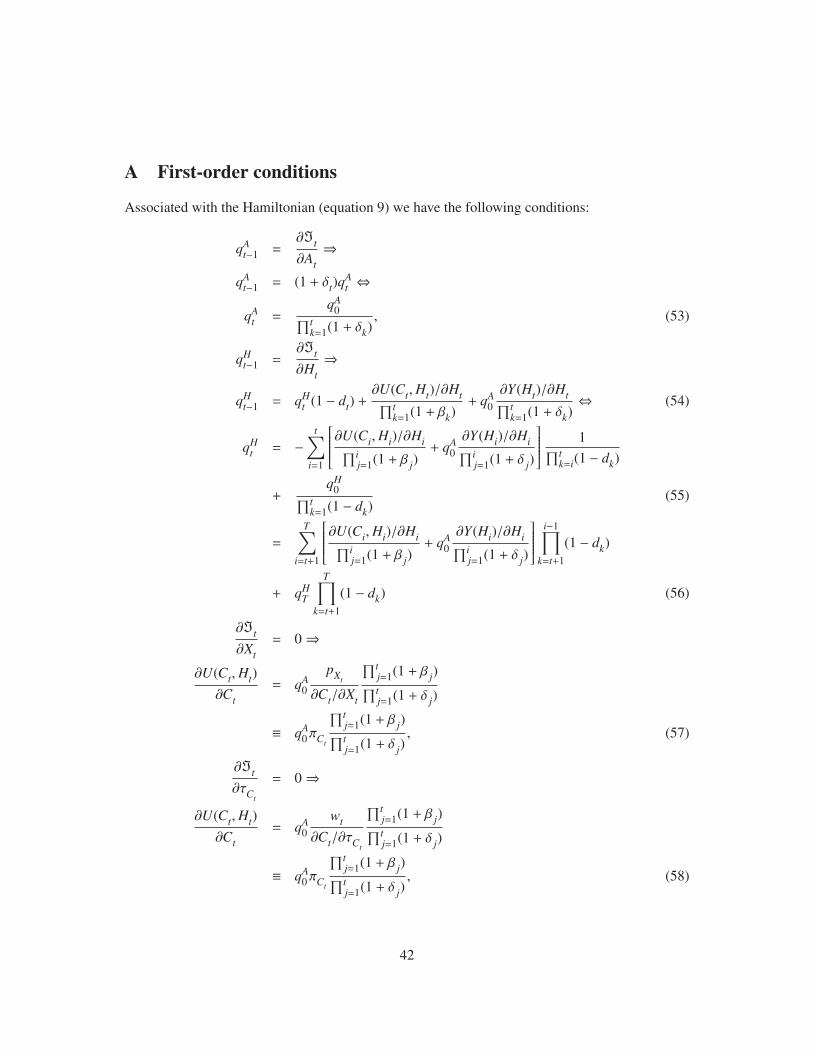
A First-order conditions

Associated with the Hamiltonian (equation 9) we have the following conditions:

qAt−1 =

∂�t

∂At⇒

qAt−1 = (1 + δt)q

At ⇔

qAt =

qA0∏t

k=1(1 + δk), (53)

qHt−1 =

∂�t

∂Ht⇒

qHt−1 = qH

t (1 − dt) +∂U(Ct,Ht)/∂Ht∏t

k=1(1 + βk)+ qA

0

∂Y(Ht)/∂Ht∏tk=1(1 + δk)

⇔ (54)

qHt = −

t∑i=1

⎡⎢⎢⎢⎢⎢⎢⎣∂U(Ci,Hi)/∂Hi∏ij=1(1 + β j)

+ qA0

∂Y(Hi)/∂Hi∏ij=1(1 + δ j)

⎤⎥⎥⎥⎥⎥⎥⎦ 1∏tk=i(1 − dk)

+qH

0∏tk=1(1 − dk)

(55)

=

T∑i=t+1

⎡⎢⎢⎢⎢⎢⎢⎣∂U(Ci,Hi)/∂Hi∏ij=1(1 + β j)

+ qA0

∂Y(Hi)/∂Hi∏ij=1(1 + δ j)

⎤⎥⎥⎥⎥⎥⎥⎦i−1∏

k=t+1

(1 − dk)

+ qHT

T∏k=t+1

(1 − dk) (56)

∂�t

∂Xt= 0⇒

∂U(Ct,Ht)

∂Ct= qA

0

pXt

∂Ct/∂Xt

∏tj=1(1 + β j)∏tj=1(1 + δ j)

≡ qA0πCt

∏tj=1(1 + β j)∏tj=1(1 + δ j)

, (57)

∂�t

∂τCt

= 0⇒

∂U(Ct,Ht)

∂Ct= qA

0

wt

∂Ct/∂τCt

∏tj=1(1 + β j)∏tj=1(1 + δ j)

≡ qA0πCt

∏tj=1(1 + β j)∏tj=1(1 + δ j)

, (58)

42

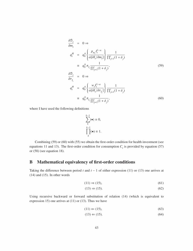
∂�t

∂mt= 0⇒

qHt = qA

0

⎧⎪⎪⎪⎨⎪⎪⎪⎩pmt

I1−αt

α[∂It/∂mt]

⎫⎪⎪⎪⎬⎪⎪⎪⎭ 1∏tj=1(1 + δ j)

≡ qA0 πIt

1∏tj=1(1 + δ j)

, (59)

∂�t

∂τIt

= 0⇒

qHt = qA

0

⎧⎪⎪⎨⎪⎪⎩ wtI1−αt

α[∂It/∂τIt]

⎫⎪⎪⎬⎪⎪⎭ 1∏tj=1(1 + δ j)

≡ qA0 πIt

1∏tj=1(1 + δ j)

, (60)

where I have used the following definitions

k−1∑k

(•) ≡ 0,

k−1∏k

(•) ≡ 1.

Combining (59) or (60) with (55) we obtain the first-order condition for health investment (see

equations 11 and 13). The first-order condition for consumption Ct is provided by equation (57)

or (58) (see equation 18).

B Mathematical equivalency of first-order conditions

Taking the difference between period t and t − 1 of either expression (11) or (13) one arrives at

(14) and (15). In other words

(11)⇒ (15), (61)

(13)⇒ (15). (62)

Using recursive backward or forward substitution of relation (14) (which is equivalent to

expression 15) one arrives at (11) or (13). Thus we have

(11)⇐ (15), (63)

(13)⇐ (15). (64)

43

Naturally, this result is also true in a continuous time formulation. In this case the first-order

condition for health investment It can be written as (notation follows the discussion in section 2)

πI(t)e− ∫ t

0δ(u)du = πI(0)e

∫ t0

d(u)du

−∫ t

0

[1

qA(0)

∂U(s)

∂H(s)e−

∫ s0β(u)du + ϕH(s)e−

∫ s0δ(u)du

]e∫ t

s d(u)duds, (65)

or, in terms of the terminal point t = T

πI(t)e− ∫ t

0δ(u)du = πI(T )e−

∫ T0δ(u)du e−

∫ Tt d(u)du

+

∫ T

t

[1

qA(0)

∂U(s)

∂H(s)e−

∫ s0β(u)du + ϕH(s)e−

∫ s0δ(u)du

]e−

∫ st d(u)duds. (66)

Differentiating (65) or (66) with respect to t one obtains

∂U(t)∂H(t)

= qA(0)[σH(t) − ϕH(t)

]e∫ t

0[β(s)−δ(s)]ds. (67)

Using the Leibniz integral rule to differentiate (analogous to taking the difference between two

time periods in discrete time) the first-order condition for health investment (65) or the alternative

expression (66) with respect to t one obtains the alternative expression (67). In other words

(65)⇒ (67), (68)

(66)⇒ (67). (69)

From (67) we obtain a first-order differential equation in πI(t)

∂πI(t)∂t

= πI(t)[d(t) + δ(t)] − ϕH(t) − ∂U(t)∂H(t)

1

qA(0)e−

∫ t0

[β(u)−δ(u)]du, (70)

which can be solved (analogous to backward or forward substitution in discrete time)

πI(t) = πI(t′)e

∫ tt′ [d(u)+δ(u)]du

−∫ t

t′

[1

qA(0)

∂U(s)

∂H(s)e−

∫ s0

[β(u)−δ(u)]du + ϕH(s)

]e∫ t

s [d(u)+δ(u)]duds. (71)

For t′ = 0 we obtain (65) and for t′ = T we obtain (66). Thus we have

(65)⇐ (67), (72)

(66)⇐ (67). (73)

44

C Variation in initial assets

Consider a variation in initial assets as in (23). The first order condition for health investment (15)

∂U∂H

∣∣∣∣∣Ct+ΔCt,A,Ht+ΔHt,A

=

{πIt

∣∣∣∣It+ΔIt,A,Ht+ΔHt,A

(dt + δt) − ΔπIt

∣∣∣∣It+ΔIt,A,Ht+ΔHt,A

(1 + δt) − ϕHt

∣∣∣∣Ht+Δt,A

}

×(qA

0 + ΔqA0,A

) ∏tj=1(1 + β j)∏tj=1(1 + δ j)

, (74)

leads, using a first-order Taylor expansion, to the following expression

∂2U∂C∂H

∣∣∣∣Ct ,Ht

∂U∂H

∣∣∣Ct ,Ht

ΔCt,A =ΔqA

0,A

qA0

+

⎡⎢⎢⎢⎢⎢⎢⎢⎢⎢⎢⎣∂πI∂H

∣∣∣∣It ,Ht

(dt + δt) −∂ϕH∂H

∣∣∣∣Ht

σH

∣∣∣It ,Ht− ϕH

∣∣∣Ht

−∂2U∂H2

∣∣∣∣Ct ,Ht

∂U∂H

∣∣∣Ct ,Ht

⎤⎥⎥⎥⎥⎥⎥⎥⎥⎥⎥⎦ΔHt,A

+

∂πI∂I

∣∣∣∣It ,Ht

(dt + δt)

σH

∣∣∣It ,Ht− ϕH

∣∣∣Ht

ΔIt,A, (75)

where I have omitted second-order terms.46

Similarly, from the first order condition for consumption (18)

∂U∂C

∣∣∣∣∣Ct+ΔCt,A,Ht+ΔHt,A

=(qA

0 + ΔqA0,A

)πC

∣∣∣Ct+ΔCt,A,Ht+ΔHt,A

∏tj=1(1 + β j)∏tj=1(1 + δ j)

, (76)

we have ⎛⎜⎜⎜⎜⎜⎜⎜⎜⎜⎜⎝∂πC∂C

∣∣∣∣Ct ,Ht

πC

∣∣∣Ct ,Ht

−∂2U∂C2

∣∣∣∣Ct ,Ht

∂U∂C

∣∣∣Ct ,Ht

⎞⎟⎟⎟⎟⎟⎟⎟⎟⎟⎟⎠ΔCt,A = −⎛⎜⎜⎜⎜⎜⎜⎜⎜⎜⎜⎝∂πC∂H

∣∣∣∣Ct ,Ht

πC

∣∣∣Ct ,Ht

−∂2U∂C∂H

∣∣∣∣Ct ,Ht

∂U∂C

∣∣∣Ct ,Ht

⎞⎟⎟⎟⎟⎟⎟⎟⎟⎟⎟⎠ΔHt,A −ΔqA

0,A

qA0

. (77)

Last, combining (75) with (77) to eliminate ΔCt,A we obtain (24).

D Structural relations for empirical testing

From the utility function (27) and the first-order conditions (15) and (18) it follows that

Ct =ζ

1 − ζσHt− ϕHt

πCt

Ht, (78)

46Such as, e.g., terms in (∂ΔπI/∂I)|It ,HtΔIt,A and ΔqA

0,A(∂πI/∂H)|It ,HtΔHt,A.

45

and

Ht = (1 − ζ)Λ(qA0 )−1/ρ

(σHt− ϕHt

)−χπχ−1/ρCt

∏tj=1(1 + β j)

−1/ρ∏tj=1(1 + δ j)

−1/ρ, (79)

Ct = ζΛ(qA0 )−1/ρ

(σHt− ϕHt

)1−χπχ−1/ρ−1Ct

∏tj=1(1 + β j)

−1/ρ∏tj=1(1 + δ j)

−1/ρ, (80)

where Λ and χ are defined in (41) and (42).

Using equations (12) and (30) we have

πIt=

p1−kImt

wkIt

α kkII (1 − kI)

1−kI μIt

I1−αt ≡ π∗It

I1−αt , (81)

mt =

(1 − kI

kI

)kI

μ−1It

p−kImt

wkIt It ≡ m∗It

It, (82)

τIt=

(1 − kI

kI

)−(1−kI )

μ−1It

p1−kImt

w−(1−kI )

t It ≡ τ∗ItIt. (83)

Using equations (19) and (31) we have

πCt=

p1−kCXt

wkCt

kkCC (1 − kC)1−kC μCt

, (84)

Xt =

(1 − kC

kC

)kC

μ−1Ct

p−kCXt

wkCt Ct ≡ X∗Ct

Ct, (85)

τCt=

(1 − kC

kC

)−(1−kC)

μ−1Ct

p1−kCXt

w−(1−kC)

t Ct ≡ τ∗CtCt. (86)

From (16), (29), (79), (81) and (84) follows

a1t I1−α

t − (1 − α)I1−αt It = a2

t H−1/χt + a3

t H−(1+γ)t , (87)

where

a1t ≡

[dt + δt − (1 − kI)pmt

− kIwt + μIt

], (88)

a2t ≡

[(1 − ζ)Λ(qA

0 )−1/ρ]1/χ

(π∗It)−1(πCt

)1−1/ρχ

∏tj=1(1 + β j)

−1/ρχ∏tj=1(1 + δ j)

−1/ρχ, (89)

a3t ≡ wt(π

∗It)−1Ω∗, (90)

where the notation ft is used to denote the relative change ft ≡ 1 − ft−1

ftin a function ft and we

have assumed small relative changes in the price of medical care pmt, wages wt and the efficiency

of the health investment process μIt.

46

Using (82) and (87) and the functional relations defined in section 3.3.1 we obtain a structural

relation (35) between health investment goods and services mt purchased in the market and the

stock of health Ht.

47