a convex programming approach for generating guaranteed passive approximations to tabulated...

IEEE TRANSACTIONS ON COMPUTER-AIDED DESIGN OF INTEGRATED CIRCUITS AND SYSTEMS, VOL. 23, NO. 2, FEBRUARY 2004 293

A Convex Programming Approach for GeneratingGuaranteed Passive Approximations to

Tabulated Frequency-Data

Carlos P. Coelho, Joel Phillips, and L. Miguel Silveira

Abstract—In this paper, we present a methodology for generatingguaranteed passive time-domain models of subsystems described bytabulated frequency-domain data obtained through measurement orthrough physical simulation. Such descriptions are commonly used torepresent on- and off-chip interconnect effects, package parasitics, andpassive devices common in high-frequency integrated circuit applications.The approach, which incorporates passivity constraints via convexoptimization algorithms, is guaranteed to produce a passive-system modelthat is optimal in the sense of having minimum error in the frequencyband of interest over all models with a prescribed set of system poles.We demonstrate that this algorithm is computationally practical forgenerating accurate high-order models of data sets representing realistic,complicated multiinput, multioutput systems.

Index Terms—Behavior modeling, convex optimization, convex program-ming, interconnect modeling, rational fitting, system identification.

I. INTRODUCTION

As system integration evolves and tighter design constraints must bemet, it becomes necessary to account for the nonideal behavior of in-creasing numbers of elements in integrated circuit systems. In systemsoperating at high frequencies, such as RF, high-speed digital, and opto-electronic interface circuits, the nonideal effects can have complicatedfrequency dependence that must be accurately modeled. Reliable de-sign tools must be available that accurately account for the behaviorof both designed-in devices, such as integrated inductors and surfaceacoustic wave (SAW) filters, as well as parasitics, such as package ef-fects. Frequently, these tools must simulate behavior in the time-do-main and time-domain system verification is made difficult since oftenonly frequency-domain descriptions of these subsystems are available.Furthermore, it is normally the case that such descriptions involve tab-ulated frequency-dependent scattering parameter or admittance ma-trices. Usually, the available data is sampled, incomplete, noisy, andcovers only a finite range of the spectrum, which makes fitting a modelto the data a difficult task.

One approach to time-domain simulation of frequency-described de-vices is to synthesize a state-spacemodel whose frequency behavior ap-proximates the original device in the frequency band of interest. Manyapproaches have been proposed for the related problems of model gen-eration, rational approximation, and system identification (for surveyssee [1] and [2]). Very roughly speaking, the most widely used tech-niques for generation of general-purpose linear models are based onleast-squares rational approximations [3]–[12] and the specific tech-niques differ in the ways of fitting the data and means of enhancing

Manuscript received May 3, 2002; revised October 16, 2002 and January 24,2003. This paper was recommended by Associate Editor C.-J. R. Shi.

C. P. Coelho is with INESC ID/Cadence European Laboratories, 1000 Lisboa,Portugal, and also with the Department of Electrical Engineering and ComputerScience, Massachusetts Institute of Technology, Cambridge, MA 02139 USA(e-mail: [email protected]).

J. Phillips is with Cadence Berkeley Laboratories, Cadence Design Systems,San Jose, CA, 95134 USA (e-mail: [email protected]).

L. M. Silveira is with INESC ID/Cadence European Laboratories, 1000–029Lisboa, Portugal, and also with the Department of Electrical and Computer En-gineering, IST—Technical University of Lisbon, 1000–029 Lisboa, Portugal(e-mail: [email protected]).

Digital Object Identifier 10.1109/TCAD.2003.822107

numerical robustness. Other popular techniques include pointwise col-location [13], moment-based approaches [4], [14], [15], and subspacemethods [16], [17].

In the model-generation problem, there are several subproblems,which consistently reappear: numerical stability of the procedure,accuracy and convergence of the approximation, stability of the model,and compactness of the representation. It seems fairly straightforwardat this point to achieve moderate accuracy when approximating lowto moderate order systems, and to do so while guaranteeing internalstability. Some algorithms use postprocessing techniques to achievestability, the most common technique being to delete unstable poles orreflect them into the left half-plane, then refit the now-stable model toregain accuracy [3], [14], [16], but a priori enforcement of stabilityis also possible [10], [16]. With some effort, it is possible to providesufficient numerical robustness to allow generation of models ofvery high order (more than a hundred poles) at high accuracy with amoderate computational cost [18]. In particular, we point out the useof orthogonal basis techniques [18], [19] that remove the intrinsicill-conditioning from approximation procedures, and the existenceof robust fixed-point and optimization procedures [18], [20] for poleestimation. It is also understood how to remove redundancy frommodel descriptions, in order to achieve the most compact modelpossible, via model-reduction procedures that can preserve passivityconstraints in the final models [21], [22]. However, at this point, nosingle scheme that we are aware of can simultaneously satisfy all theconstraints on a practical method, particularly in a design-automationenvironment where engineers who wish to generate models frommeasured data are not likely to be experts in rational approximation.

Our main concern in this paper is to generate models that are well-behaved when used in later time-domain simulation. Typically, the bestway to ensure good model behavior is to require that the state-spacemodels not only have frequency responses that match the available data,but that they also possess stability and passivity properties similar tothose of the physical system that they represent. Specifically, we seekpassive models of passive systems. Otherwise, nonphysical anomaliesmay be introduced into the time-domain simulation. In the worst case,the time-domain simulation may become unstable and exhibit rapid,exponentially growing, oscillations in the simulated waveforms.

In this paper, we present our latest progress toward an efficient algo-rithm that can produce guaranteed passive models by construction. Weseek an approach with rigorous, global guarantees on positive-realness,thus, passivity, whose accuracy loss due to imposition of the passivityconstraint is as small as possible. The approachwe describe here is opti-mization-based and assumes that a stable matrix rational function (i.e.,a state-space model with poles in the left half of the complex plane)has already been generated, and that the pole estimates are sufficientlygood for the desired level of approximation accuracy. Any convenientrational approximation algorithm [1], [2], [16], [18], [20] can be usedto generate this initial approximation. The remaining model quantities(the matrix “numerator”) are then recalculated such that the error be-tween the original data set and the model’s frequency response is min-imized under the constraint that the model be passive. The passivityconstraint is imposed by requiring that the state-space model that is fitsatisfies the positive-real lemma.

With this approach, the objective function and the constraints areconvex functions of the optimization variables, so convex programmingalgorithms can be applied [23]. These algorithms are guaranteed to findan optimal solution, thus generating the best rational approximationpossible under the constraints of passivity and a given pole structure.Failure of the algorithm provides proof that either the pole estimateswere “bad,” or the data cannot be approximated by a passive model.

0278-0070/04$20.00 © 2004 IEEE

294 IEEE TRANSACTIONS ON COMPUTER-AIDED DESIGN OF INTEGRATED CIRCUITS AND SYSTEMS, VOL. 23, NO. 2, FEBRUARY 2004

This paper is structured as follows. In the next section, we providebackground information on passive systems and positive realness. InSection III, we present the efficient formulation of the positive real con-strained multivariable fitting problem. Section IV considers aspects ofpractical implementation of the techniques, particularly considerationsinvolved when using the special model structures proposed in [18] and[20], and comparisons to suboptimal approximation strategies. Finally,in Section V, experimental results illustrating the use of the proposedformulations to generate models for several real-world examples arepresented.

II. CONSTRAINTS FOR PASSIVE-MODEL GENERATION

A. Passivity and Positive-Realness

Many physical systems (such as networks composed of resistors, ca-pacitors and inductors) are passive, meaning that they do not generateenergy. Interconnected passive systems are passive [24]. Stable systemsdo not possess this closure property. This distinction between stable andpassive systems is of immense importance when generating models forsimulation. A stable model, composed with other stable or even passivemodels, may not lead to a stable system and may lead to nonphysical orunstable simulations, depending on the properties of the other modelsand the overall system the models are connected to. This instabilitycannot be predicted at the time the model is created. In contrast, if amodel of a passive system is passive, it is then known that the modelin and of itself cannot result in unstable simulations. Therefore, our al-gorithm must incorporate appropriate conditions for the model to beguaranteed passive.

The admittance and impedance parameter matrices of passive elec-trical networks are positive real matrix rational functions [25]. A squarematrix functionH(s) is said to be positive real if it satisfies

H(s) is analytic; for Re[s] > 0 (1)

H(s) = H(�s); for Re[s] > 0 (2)

H(s) +H(s)H � 0; for Re[s] > 0: (3)

Similarly, if a scattering-parameter matrix formulation is used, H(s)must be bounded real; condition (3) is replaced by I�HH(s)H(s)�0 for Re[s] > 0. In the above,H denotes complex conjugate,HH de-notes Hermitian transpose, and�0 in amatrix context denotes semidef-initeness. For further references on passivity and the more general con-cept of dissipativity see, for example, [24] and [26]–[30].

Much previous work on passive-model generation attempts to usepoint-by-point frequency-domain positive-real conditions directly. Acommon misconception is that if the given data is passive, then a suf-ficiently good fit to the data will result in a passive model, or that pas-sivity can be assured by introducing additional grid points (points at dc,at infinite frequency, points in between) where passivity is enforced.Fundamentally, however, fitting data at a set of discrete points does notgenerally represent a strong enough constraint to ensure positive- orbounded-realness over the entire axis1 as the behavior of the model out-side the data range, or between the points, cannot be controlled. Amoresubtle problem with nonglobal constraints is that since the best-fit pas-sive model can never be a better fit than the best-fit nonpassive model,an optimal fitting process will tend to choose models that trade pas-sivity for goodness of fit. That is, even if the model satisfies the localconstraints, it is likely to be globally nonpassive, such as by being non-passive at high frequencies, well outside the given data range, or be-tween the highest finite data-point frequency and “infinite” frequency.

1See [27] and [31] for an example, in a scalar context, of a sufficiently strongpointwise constraint.

Ironically, this sort of problem is unlikely to be detected by visual in-spection of the frequency-domain model, but will create considerablehavoc in time-domain simulation.

Recently proposed model-generation techniques utilize local posi-tive-realness constraints at a finite number of discrete points [32]–[37]combined with heuristic band-limiting [32], [33] arguments, possiblywith additive compensation of the transfer function in-[35] and/or out-[34] of the approximation interval. Therefore, passivemodels cannot beguaranteed in all cases, or require introducing additional constraints onthe behavior of the transfer function. These constraints can be difficultto remove, leading to models that are not as compact as possible. An-other class of approaches enforces global positive-definite constraintson individual subsystems (such as pole-residue pairs) [38], [39] thatsum together to form the transfer function. Requiring that each sub-system be positive-real ensures that the sum is positive-real in turn, butwe shall show that it also over-constrains the modeling problem whichmay lead to inaccurate models.

An effective model generation procedure must be based on a con-straint that guarantees positive- (or bounded-) realness of the transferfunction at all points on the imaginary axis, but should not over-con-strain the approximation problem. The constraint must admit all modelsthat are passive, otherwise, it would be possible to generate data setsthat cannot be fit accurately. The approaches in [32], [33], and [35] donot satisfy the first condition and the methods in [33], [34], [38], and[39] do not satisfy the second. We desire a constraint that can ensureglobal positive-realness, but that is only as restrictive as necessary, i.e.,within the model class it should be both sufficient and necessary.

B. Positive-Realness Constraints

We now review formulation of sufficient and necessary conditionsfor passive-model generation. In the remainder of the paper, withoutloss of generality, we will work with admittance/impedance-parameterdescriptions of networks, whose transfer functions must be positive-real. In this paper, we will be mainly concerned with matrix rationalfunctions that originate from state-space models

dx

dt= Ax(t) +Bu(t); y(t) = Cx(t) +Du(t) (4)

for generic multiinput, multioutput systems, with transfer functionH(s) = D+C(sI�A)�1B. Here, generically, for a system with minputs andm outputs,A 2

n�n is the state matrix,B 2 n�m is theinput matrix, C 2

m�n is the output matrix, andD 2m�m is the

direct term, giving instantaneous input-output interaction. The centraltool in relating passivity of state-space models to positive-realness ofthe transfer function is the Positive Real Lemma [26], [30].Theorem 1 (Positive Real Lemma): Let (A;B;C;D) describe a

state-space model whose transfer function is given by H(s) = D +C(sI � A)�1B. For simplicity, we will require that the state-spacesystem described by (A;B;C;D) be controllable.2 Further, supposethat H(s) has all of its poles either in the left-half plane or on theimaginary axis, in which case they are simple. If there exists aK = KT

such that the linear matrix inequalities (LMIs)

�ATK�KA �KB+CT

�BTK+C D+DT� 0 (5)

K � 0 (6)

are satisfied, thenH(s) is positive-real. Conversely, ifH(s) is positive-real, then the LMIs (5)–(6) are feasible, i.e., aK exists such that (5)–(6)are satisfied.

2Posing positive-realness via the dual of these equations would have observ-ability as a necessary condition.


One special case and one extension remain to be mentioned. First,suppose it is desired to constrainD = 0. The inequality in (5) shouldbe replaced by

�ATK�KA � 0 and KB = CT

: (7)

Second, suppose it is desired to include the term proportional to s inthe transfer function, so thatH(s) = sY1 +D +C(sI �A)�1B.For positive-realness, the term sY1 must be lossless [28]; Y1 mustsatisfy

Y1 = Y1;T

; Y1 � 0 (8)

and in addition the remaining proper part of the transfer function,D+C(sI �A)�1B, must be positive-real, i.e., A;B;C;D must satisfy(5)–(6).

III. CONVEX OPTIMIZATION STRATEGY

In this section, we will describe our methodology for generatingguaranteed passive time-domain models of frequency-described sub-systems. Our strategy is based on two fundamental observations. First,over the past decade, empirical evidence has accumulated to indicatethat stable rational approximations of tabulated data may be generatedat moderate computational cost. We have previously demonstrated [18]algorithms for numerically robust, stable approximation of very com-plicated data with high-order (more than 100 poles) models. Second,we note that the positive-real constraints are affine (thus convex) in bothC and D. This suggests an algorithm based on a fixed pole structure,i.e., fixed A, that computes C and D in such a way that the overallmodel is passive and meets the approximation constraints. Estimationof a fixedB is also required for this approach, however, as we shall seein Section IV-A, with a particular implementation choice we can avoidestimation of B as well. Since the LMI constraints are convex, with aconvex formulation of the error constraints, we can obtain an algorithmthat can find an optimal approximation in polynomial time [40].

Therefore, as the starting point of our algorithm, we assume that asuitable pole structure is available. The pole estimates could come froma variety of sources, and it it not critical to our approach from whencethey come. A likely possibility is that an initial rational approximationhas been performed, but this approximation is not positive-real. Otherpossible sources for the pole structure include Laguerre-type models[41] and nonlinear eigenvalue problems [42]. It is, therefore, assumedthat a stable matrix rational function (i.e., a state-space model with nopoles in the right half of the complex plane) has already been gener-ated, and that the pole estimates are sufficiently good for the level ofapproximation accuracy desired. Any convenient rational approxima-tion algorithm [1], [2], [18], [19], [43] can be used to generate this ini-tial approximation. There is reasonable hope to believe in the successof the overall approach, since, for an accurate rational approximationto be generated, it must have been possible to have good pole estimatesfor the poles that are relevant to the frequency band of interest.

Care should be taken to distinguish our proposed strategy from the“nearest positive-real model” techniques proposed in [36], [37], and[44]. We advocate computing a first model (not necessarily positive-real), retaining the poles, and then recomputing a positive-real modelthat is a best fit to the original data, whereas in the “nearest positive-realmodel” approach, the second model is chosen “close” to the first, non-passive model. This approach can lead to very inaccurate models, be-cause the stable, but not passive, model may have large deviations frompassivity out-of-band, much larger than its deviations from the datain-band. The “nearest positive-real model” can be a very poor matchto the original data, because it must try to compensate for the large (butirrelevant) deviations from positive-realness of the first model.

Next, we formulate the optimization problem.

A. Formulating Optimization Objectives

Assume that we are given admittance or impedance parameter ma-trices of a system ~H(s) for a set ofN frequency points s1 through sNand that a stable matrix rational-function model already exists.

Let Hp;q(s) denote the (p; q) entry of the model transfer functionH(s) = D+sY1+C(sI�A)�1B. Let ~Hp;q(sk) be the measuredvalue of the data for entry (p; q) at the kth frequency point. Let k from1 to N and, for simplicity and without loss of generality, let p; q eachrange from 1 tom, wherem is thus the number of inputs and of outputsof the system.

The problem at hand is to determine C;D;Y1 such that a costfunction is minimized, with constraints on the errorHp;q � ~Hp;q . Themost common constraints are entry-wise absolute-error constraints andconstraints on the weighted least-squares error, taken over frequency

N

k=1

wk;p;qkHp;q(sk)� ~Hp;q(sk)k2

2 < tp;q: (9)

Because N may be large, (9) may lead to a very large number of con-straints. For example, we will be interested in treating problems whereN > 1000 and p; q range from 2 up to 12. In these cases, it is desir-able to generate the most compact form possible for the constraints.The least-squares constraint in particular can be further compressed.

LetBq denote the qth column ofB and, likewise, letCp denote thepth row ofC, so thatHp;q(sk) = sY1p;q+Dp;q+Cp(skI�A)�1Bq.LetDq;Y

1

q denote the qth column ofD;Y, respectively. Let ep de-note the pth column of the identify matrix. Let Fp;q 2 2N�m andGp;q 2

2N be defined as (for the kth row)

Fp;q(k; :) =wp;q;kRe[J(sk)] k � N

wp;q;k�NIm[J(sk�N)] k > N(10)

Gp;q(k) =wp;q;kRe[ ~Hp;q(sk)] k � N

wp;q;k�NIm[ ~Hp;q(sk�N)] k > N(11)

where

J(s) = BTq (Isk �A

T )�1eTq seTq :

Also, let Xp be the pth column of

X =

CT

DT

(Y1)T: (12)

Now, we can writeN

k=1

wk;p;qkHp;q(sk)� ~Hp;q(sk)k2

2 = kFp;qXp �Gp;qk: (13)

Now, let us perform the decomposition

Qp;qRp;q = Fp;q (14)

whereQTQ = I andR is full rank, via a singular value decompositionor rank-revealing QR factorization. We now have

jFp;qXp �Gp;qj = (Fp;qXp �Gp;q)T (Fp;qXp �Gp;q)

= ETp;qEp;q + �2

p;q (15)

where

�2

p;q = GTp;q(I�Qp;qQ

Tp;q)Gp;q (16)

and

Ep;q = (Rp;qXp �QTp;qGp;q): (17)

With these definitions, the least-squares constraint (9) becomes

ETp;qEp;q + �

2

p;q � tp;q: (18)

We have written these equations using only real quantities, therebyconstrainingC;D;Y1 to be real as well. The quantity �p;q has an in-


teresting interpretation. In the absence of positive-realness constraints,�p;q would be the minimal achievable error obtainable, were we to cal-culate the optimalC;D;Y1 in an entry-wise fashion, i.e., to treat each~Hp;q(sk) as a single-input, single-output (SISO) system. Because in amultiinput, multioutput (MIMO) system the entries are not indepen-dent, and because positive-realness introduces additional constraints,�p;q will turn out to give a lower bound on the achievable accuracy ofthe fit.

With this notation, we can state the optimization problem as

minimize t(C;K;D;Y1)

subject to : Eqs. (5), (6), (8)ETp;qEp;q + �2p;q � tp;q

t � 0

tp;q � tfor 1�p;q�m

: (19)

It should be clear that we could choose many other optimizationgoals. For example, minimizing the maximum least-squares error overthe transfer function entries. We may also fix t at some acceptablevalue, thus bounding themaximum allowable error, andminimize someother function of the free variables. For example, minimizing Tr(K)(where Tr() denotes the trace of a matrix) is a possible strategy toachieve a minimal degree solution with bounded error.

It is sometimes desirable to introduce additional constraints on thevariables [C;D;Y1]. For example, we may wish to fix D or Y1

to a specific value, such as zero, or a value chosen to enforce specificbehavior at infinite frequency, or at dc. Such a fixed value must, ofcourse, be admissible, i.e., satisfyD+DT

� 0 or (8) as appropriate.It is tempting to suggest estimating an admissible D or Y1 a priori,subtracting it from the initial data, and fitting the remainder with a pos-itive-real function [35], but this approach leads to suboptimal fits. In-stead, we introduce additional linear constraints into the optimizationformulation, or create a parameterization of the solution vectorX thatincludes the constraint.

B. Semidefinite Formulation and Solution

In (19), both the objective function and the constraints are convexfunctions of tp;q;K;C;D, andY1. The most straightforward way tosolve these equations is to use the Schur complement [23] to transformeach quadratic inequality in (19) to a linear matrix inequality (LMI),e.g., (18) may be transformed to

tp;q � �2p;q ETp;q

Ep;q I� 0: (20)

This optimization problem can be solved using standard semidefiniteprogramming techniques [45], as was proposed in [46]. The resultsobtained showed that the cost of computing the models, measured asthe number of floating point operations, exhibited rapid growth withn, the order of the state-space model. This is primarily because thepositive-real and Schur-form error LMI constraints introduce a largenumber of constraints, and the introduction of the K variable causesthe number of unknowns to grow quadratically with model order. Infact, the cost of forming the matrix needed to compute the step direc-tion in each iteration of the optimization procedure is roughly O(n6)if no structure or sparsity is exploited. Thus, although the semidefiniteprogram (SDP) problem formulation and solution procedure is straight-forward, its use is limited to relatively small problems, n � 20 or so.

C. Structure-Exploiting Formulation (SEF) and Solution

One way to reduce the cost of solving the convex optimizationproblem is to seek a more efficient formulation of the constraint func-tions. Several structure-exploiting techniques [47]–[49] for solvingoptimization problems with LMI constraints have recently beenproposed. We have adopted an approach with a reparameterization

similar to that suggested in [44] for the SISO case. Further exploitationof the positive-real problem structure motivated by [47], along withadditional initial transformations, allow us to reformulate the problemin a form that enables sparsity to be exploited in the computations.

The first step to a more efficient procedure is to reformulate theproblem to remove the explicit LMI constraint (5). Consider again thepositive-realness constraint, which by introducing a matrix Z may bewritten as

Z = ZT =Z11

Z12

(Z12)T Z22

=�A

TK�KA �KB+CT

�BTK+C D+DT � 0: (21)

If the system described by [A;B;C;D] is positive-real, then a Z > 0exists. Again, recalling that A;B are fixed, we note that the set ofZ (which is convex) parameterizes the set of feasible C;D. We willuse this idea to preeliminate the constraint (5) from the optimizationproblem. Let us suppose we are given such a Z. Then,

�ATK�KA = Z11

: (22)

This is a Lyapunov equation for K. Given A and Z11;K is uniquelydetermined.We use vec, mat notation, andKronecker product identities[50] to write a closed-form solution to (22). Recall that the vec operatorforms a vector from a matrix by stacking its columns

veca11 a12

a21 a22=

a11

a21

a12

a22

(23)

and that the mat operator reverses this operation. The Kroneckerproduct of two matrices J 2 m�n;K 2 p�q is the block matrixJ K 2

mp�qn

JK =

J11K J12K � � � J1nK

J21K J22K � � �...

. . .

Jm1K � � � JmnK

: (24)

The basic Kronecker product identity for matrix equations is

JKL =M ! (LT J) vec(K) = vec(M): (25)

Inner products in the matrix space may be notated as

vec(A)T vec(B) = Tr(ATB) (26)

where Tr() denotes trace, when convenient.With this notation, (22) is equivalent to

T vec(K) = vec(Z11) (27)

where T = �I AT�A

T I, so that

K = mat T�1vec(Z11) : (28)

This parameterizesK as in [44], but for our problem, a more efficientparameterization is available. Noting that

CT = KB+ Z12 (29)

and that the optimization constraints (17) and (18) involve C, we seethat what is desired is a parameterization ofKB directly.

Specifically, for each r; p, we desire a matrix Pr;p such that the r; pentry of KB is given by (KB)r;p = Tr(Pr;pZ) = �Tr;pvec(Z) forsome vector �Tr;p [we used the identity in (26)]. Now, since

vec(KB) = (BT I)vec(K) (30)

= (BT I) T�1vec(Z11) (31)

= (T�T B I)T

vec(Z11) (32)


then noting that each column of B I is of the form Bp er , whereBp is the pth column of B, and er is the rth unit vector, we see that

�r;p = T�T (Bp er): (33)

By introducing the matrix Pr;p = mat(�r;p), which will be conve-nient below, we may also write

Pr;p = mat(�r;p) = mat T�T (Bp er) (34)

or, if we seek a solution where Pr;p is symmetric

Pr;p = mat T�T (Bp er) + mat T�T (Br eq)T

: (35)

Note that, by letting Pr;p = mat(T�T (Bp er));Pr;p can be ob-tained by solving the Lyapunov equation

APr;p +Pr;pAT = �Bpe

Tr (36)

and then taking the symmetric solution. Finally, since the symmetricpart of D is parameterized by Z, we only need to introduce the extravariableD(a) = �(D(a))T to represent the nonsymmetric part ofD.Then, we have a complete formulation for positive-real constrained ap-proximation with fixed A;B:

minimize t(Z;Y1)

subject to: t � 0; Z = ZT � 0; Y1 = (Y1)T � 0

tp;q � tEp;q = Rp;qXp �Q

Tp;qGp;q

Cp;r = �Tr;pvec(Z) + Z12r;p

Dp;q = Z22p;q +D

(a)p;q

ETp;qEp;q + �2p;q � tp;q for 1�p; q�m

: (37)

The second step to a more efficient procedure is to avoid the matrixconstraints introduced by forming the Schur complement. This is doneby recognizing that the constraint (18) is a second-order cone con-straint [51], [52]. It is more efficient to use an algorithm that treats theseconstraints directly, rather than translating to the form (20) needed forsemidefinite programming.

The remaining issues to be addressed are how the vectors � canbe computed efficiently, and if the optimization problem (37) can besolved quickly. The two questions are related. AsB 2 n�m, the costof computing the Pr;p is at most the cost of the solution of mn Lya-punov equations, which can be done in O(mn4) time using standardtechniques. This is already an improvement over [44], and of lowercomplexity than the SDP formulation. However, it is possible to im-prove this number.

The third step to a more efficient procedure is to manipulate A toa form in which the matrices � (or, equivalently, the vectors �) aresparse. This is the case if the solutions of the Lyapunov (36) are sparse.Generally, the solutions of a Lyapunov equation (Pr;p in this case) aredense, even if the matrix A is sparse. However, we are free to per-form an arbitrary state transformation to the matrixA before enteringthe fitting procedure. This is a reflection of the fact that only preser-vation of the poles is really necessary for our procedure, the coordi-nate system is irrelevant. In addition, (36) has a sparse right-hand sidematrix. For each Lyapunov equation, the matrix Bpe

Tr is nonzero in

only one column. For suitably chosen sparseA, this can lead to sparsePr;p. In particular, if A is chosen to be block-diagonal, the Pr;p willbe block-sparse. As a result, they can be computed more efficiently.For a block-diagonal matrix A of rank n with size-k blocks (so thereare n=k blocks), the cost of computing all the P is O(mk2n2). Ide-ally, we would reduce the matrixA to block-diagonal form with size-1(real pole) or size-2 (complex pole) blocks, but it is not always pos-sible to perform this computation in a numerically stable way. It ispossible, however, to reduce to blocks each of which contain well-sep-arated groups of eigenvalues [53] and such blocks are usually muchsmaller than n.

Algorithm 1 shows the final fitting procedure. As a side note, wepoint out that, while in this procedure, we do not explicitly computeK, it is easily obtained from Z11 by solving the Lyapunov (22).

Algorithm 1 SEF Matrix Fitting AlgorithmObtain matrices [A;B], withA stable, in a convenient

canonical form.Compute the matrices Pr;p from (36).Formulate the optimization problem as in (37).Solve (37) for Z;Y1 using mixed semidefinite/second-

order cone programming.Extract and return [C;D;Y1].

IV. PRACTICAL IMPLEMENTATION

A. Single-Input, Multiple-Output (SIMO) Model Representations

The formulations in the previous section apply to an MIMO of ar-bitrary structure. However, the most effective fitting algorithms we areaware of [18], [20] use models with special internal structure. In par-ticular, these methods represent MIMO systems as a set of SIMO sys-tems, because it seems that in the fitting context, the SIMO-like struc-ture achieves the best compromise between robustness, accuracy, andmodel size. Of course, the overall system is still MIMO, and the pas-sivity constraints must apply to theMIMO system, it is just the internalstructure that is SIMO-like.

The SIMO-like representation of a multivariable m-port system (minputs and m outputs) is modeled by the concatenation of m SIMOstate-space models (see [46] for details). Note that when we generatea system of this structure, with no constraints on theC-matrix entries,and no necessary relation between the blocks of A, the system willbe minimal in the generic case. However, were we to take an arbitraryexisting, minimal, MIMO system and recast it into the SIMO form, thenew (SIMO) representation will always be nonminimal. In particular,if the order of each SIMO system is n, the concatenated MIMO systemwould have (m� 1)n nonobservable modes.3

It is, therefore, reasonable to wonder if or when the fitting processcan generate nonminimal models. This turns out to be rare and, to seethis, consider the case where the model approximation is poor. Thiscan occur from poor pole estimates, or from choosing too low a modelorder. If the model was nonminimal, we could delete the offendingstates, obtaining exactly the samemodel response with exactly the sameerror, but with a lower order model. Such a model is unlikely to bethe optimum fixed-pole model of a given order, because the degreesof freedom corresponding to the deleted modes were not utilized inthe fitting process. It is possible, however, that when accurate modelsare obtained, the SIMO structure results in models with redundant in-formation, models that have some very weak modes. After the fittingis complete, we can eliminate any states with small influence on thetransfer function via a model-order reduction procedure, such as trun-cated balanced realization model-reduction techniques. Since we de-sire final models that are passive, we must use a passivity-preservingreduction algorithm [21].

A second interesting aspect of the SIMO representation is that itmakes the fixed-pole fitting procedure insensitive to the estimation ofthe B matrix. From the SIMO structure, it is clear that each columnof the transfer function can be fit independently, and introduce no con-straints on each other. Suppose that theAk;k are in diagonal form. Con-sider the (p; q) entry of the transfer function. Only the product of theentries in the vectorsCp;q andBq;q enter the expression for the transferfunction, so for any fixed Bq;q , we may obtain any desired residue byadjusting only C. Since the transfer function is invariant under sim-

3It would still be fully controllable.


ilarity transformations of the internal states, we see that, in fact, thechoice of B is arbitrary with this representation.

This is interesting since we know we will obtain, for a givenA, theoptimal choice ofC;D;Y1, and since the only invariant informationinA is the pole structure, we now conclude that if the pole locations arereasonable the algorithm is guaranteed to produce an accurate model.It also makes clear that there is no real additional advantage in using aSISO structure.

B. Suboptimal Fitting Strategies

In this section, we will discuss some schemes that seek computa-tional simplicity by avoiding the complex constraints imposed by thepositive-real lemma, but are intended to produce passive models. Gen-erally speaking, these schemes are either not guaranteed passive, orare suboptimal, in the sense that they introduce conditions that aresufficient to ensure passivity, but are not necessary. As a result, theyover-constrain the model that is generated. For simple data, particu-larly SISO data, this is often not a problem, as the additional constraintsare few and weak. However, for complex data with many input/outputpairs, the deterioration in accuracy can be severe.

First, we discuss the method in [38]. Suppose that we assume ablock-diagonal form for the matrixA. In addition, let us constrainK tohave the same block-diagonal structure. This is equivalent to requiringthat the contribution to the transfer function from each pole or pole-pairbe itself positive-real, i.e., applying the positive-real constraint to eachof the internal subsystems associatedwith each pole. In [38], theMIMOsystem was represented by multiple SISO systems, or, equivalently, theresidue matrices for each pole were allowed to be rank-m instead ofrank-1. The subsystem associated with each unique pole or pole-pairwas required to be positive-real, which again is equivalent to assuminga block-diagonal form for the matrixK, with blocks conformal to theblocks in A corresponding to unique poles. Since the methods pro-posed in Section III always generate the optimal K for a given polestructure, they will always be at least as accurate as the method of[38], and generally more accurate, since the optimalK is almost neverblock-diagonal in general coordinates. A similar analysis can be ap-plied to all other algorithms that rely on postprocessing B;C;D, orY1 to achieve passivity since these can be interpreted as special in-

stances of a fixed-pole fitting algorithm.We will now briefly discuss the incremental fitting algorithm in-

troduced in [46]. This algorithm reduces the quadratic increase of thenumber of variables with the number of ports. It was proposed that thefitting of a multiport system be split in a series of smaller problems,based on the premise that if a matrix function is positive-real, its minorsare also positive-real matrix functions. It was proposed that the fittingprocess start by approximating all the diagonal elements of the rationalfunction matrix, then determine the sub and super-diagonal blocks ofminors of increasing order on the diagonal. On average this procedurewas found to be faster by a constant factor, usually about five. However,it was found that this improvement was achieved at the occasional costof some accuracy loss, particularly in the off-diagonal elements of thetransfer function, where the fitting procedure is over-constrained.

V. RESULTS

In this section, we discuss results from applying the proposed al-gorithms to generate models of several multivariable passive systems.We used standard optimization packages to perform the experiments,SDPPack [54] for the smaller problems and SeDuMi [55] for the larger.Throughout this section, we have chosen a variety of examples and polegeneration techniques to demonstrate that we can effectively work withdifferent model structures (SISO, MIMO, SIMO, etc.), and differentstarting models (e.g., from [16], [18], and [35]).

Fig. 1. Multivariable passive constrained fit of the admittance matrix of a coilinductor. This shows the approximation to the Y entry of the admittancematrix.

Fig. 2. Passive model fit to nonreciprocal lumped circuit.

A. General Robustness, Flexibility, and Accuracy

The first examples will show the general effectiveness, robustness,and flexibility of the method. Specifically, not only does the proposedapproach generate models passive by construction, but it can be usedto obtain high-order, highly accurate approximants for complicated fre-quency-data systems.

In the first example, a 36th-order model for the admittance matrixof a two-port coil inductor is generated. First, the algorithm presentedin [18] is used to obtain an initial approximation. This approximation,while accurate, is found not to be passive. Using the techniques pro-posed in this paper, the pole estimates are kept, but the full MIMOmodel is recomputed. The frequency response of the diagonal Y2;2entry is shown in Fig. 1. Even considering the higher-order approxi-mation, the accuracy of the fit model is very good over all data points.

For our second example, we consider a lumped RLC circuit con-structed to be nonreciprocal by including a gyrator element. Initialpole estimates were generated using the approach of [35]. Results ofan order-7 constrained-rational fit are shown in Fig. 2. This exampleillustrates that our fitting and reduction approaches are valid for nonre-ciprocal systems which do not have a symmetric model representation,


(a) (b)

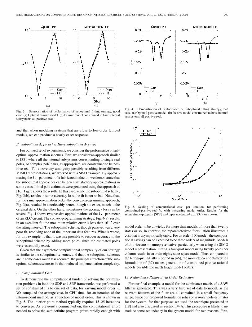
Fig. 3. Demonstration of performance of suboptimal fitting strategy, goodcase. (a) Optimal passive model. (b) Passive model constrained to have internalsubsystems all positive-real.

and that when modeling systems that are close to low-order lumpedmodels, we can produce a nearly exact response.

B. Suboptimal Approaches Have Suboptimal Accuracy

For our next set of experiments, we consider the performance of sub-optimal approximation schemes. First, we consider an approach similarto [38], where all the internal subsystems corresponding to single realpoles, or complex pole pairs, as appropriate, are constrained to be pos-itive-real. To remove any ambiguity possibly resulting from differentMIMO representations, we worked with a SISO example. By approxi-mating the Y11 parameter of a fabricated inductor, we demonstrate thatthe suboptimal approaches can be given satisfactory approximations insome cases. Initial pole estimates were generated using the approach of[16]. Fig. 3 shows the results. In this case, while the suboptimal scheme,Fig. 3(b), results in some accuracy loss, the fit is not so bad. Note that,for the same approximation order, the convex-programming approach,Fig. 3(a), resulted in a noticeably better, though not exact, match to theoriginal data. On the other hand, sometimes the accuracy loss can besevere. Fig. 4 shows two passive approximations of the Y11 parameterof an RLC circuit. The convex-programming strategy, Fig. 4(a), resultsin an excellent fit: the maximum relative error is less than 10

�4 overthe fitting interval. The suboptimal scheme, though passive, was a verypoor fit, resolving none of the important data features. What is worse,for this example, is that it was not possible to recover accuracy in thesuboptimal scheme by adding more poles, since the estimated poleswere essentially exact.

Given that the asymptotic computational complexity of our strategyis similar to the suboptimal schemes, and that the suboptimal schemesare in some casesmuch less accurate, the principal attraction of the sub-optimal schemes seems to be their reduced implementation complexity.

C. Computational Cost

To demonstrate the computational burden of solving the optimiza-tion problems in both the SDP and SEF frameworks, we performed aset of constrained fits to one set of data, for varying model order n.We computed the average cost, in CPU time, for an iteration of theinterior-point method, as a function of model order. This is shown inFig. 5. The interior point method typically requires 15–25 iterationsto converge. As previously commented on, the computational effortneeded to solve the semidefinite program grows rapidly enough with

(a) (b)

Fig. 4. Demonstration of performance of suboptimal fitting strategy, badcase. (a) Optimal passive model. (b) Passive model constrained to have internalsubsystems all positive-real.

Fig. 5. Scaling of computational cost, per iteration, for performingconstrained-positive-real-fit, with increasing model order. Results for thesemidefinite-program [SDP] and reparameterized SEF (37) are shown.

model order to be unwieldy for more than models of more than twentystates or so. In contrast, the reparameterized formulation illustrates acost that is asymptotically cubic. For an order-100 model, the computa-tional savings can be expected to be three orders of magnitude. Modelsof this size are not unrepresentative, particularly when using the SIMOmodel representation. Fitting a four-port model using twenty poles percolumn results in an order eighty state-space model. Thus, compared tothe technique initially reported in [46], the more efficient optimizationformulation of (37) makes generation of constrained-passive rationalmodels possible for much larger model orders.

D. Redundancy Removal via Order Reduction

For our final example, a model for the admittance matrix of a SAWfilter is generated. This was a very hard set of data to model, as therelevant features of the filter are all contained in a small frequencyrange. Since our proposed formulation relies on a priori pole estimatesfor the system, for that purpose, we used the technique presented in[18] and also discussed in Section IV-A. This procedure is likely to in-troduce some redundancy in the system model for two reasons. First,


Fig. 6. Multivariable passive constrained fit of the admittancematrix of a SAWfilter. Figures shows the frequency response of the Y entry for the originaldata, a full MIMO model and a the result of a passivity-preserving reductionalgorithm.

Fig. 7. Time-domain response of the nonreciprocal circuit, driven by pulsesource. Solid line: original circuit. Dash line: fourth order rational fit model.(+) seventh order rational fit model. The seventh order model is a near-exactmatch.

it is desirable to have techniques that are robust with respect to er-rors in order estimation. An effective strategy is to “over-estimate” thenumber of poles that are needed to achieve a given accuracy level, fitthe high-order model, then optimally compress it for simulation. Thisis often more practical than trying to obtain precise a priori estimatesof the order needed to fit a given data set. Second, to generate the polestructure, we used the technique presented in [18] and, as discussed inSection IV-A, when the full MIMO model starts from a concatenationof SIMO models, it is quite possible that there are system dynamicsthat, within approximation error, are taken into account more than once.(In reality, due to numerical roundoff, it is unlikely that we will see theexact same pole estimate twice. More likely, we will see two poles verynear to one another.) We, therefore, apply a model reduction step [21]as discussed in Section IV-A. For this example, the full MIMO modelis a 60th order system. In Fig. 6 we show the original data, the fre-quency response of the full (passive) MIMO model, and the frequencyresponse of a 24th order (passive) reduced-order model. As can be seen

from the plot, the accuracy of the reduced-order model is quite good:the actual accuracy of the reduced-order model is completely control-lable. This result shows that substantial reduction is attainable usingappropriate model-order reduction techniques, showing that it can bebetter to seek an accurate, passive, even if somewhat redundant, modelsince reduction is possible as a postprocessing step.

E. Time-Domain Simulation

For our final result, we show results of time-domain simulation. Weconsider the nonreciprocal circuit from Fig. 2. Fig. 7 shows a resultfrom time-domain simulation when this model is inserted into a testbench with capacitive feedback and excited by a pulse source. Botha fourth-order model, which gives a poor frequency domain fit, anda seventh order model, are shown in Fig. 7. The higher-order modelshows a good match in the time domain.

VI. CONCLUSION

In this paper, a methodology was presented for generating guaran-teed passive models of frequency-described subsystems. It was arguedthat while algorithms exist that can robustly generate an arbitrarily ac-curate approximation to a system’s admittance or impedance function,guaranteeing passivity is a harder problem. To solve it, the modelingproblem is formulated as a fixed-pole positive real constrained rationalapproximation problem which in turn is reformulated as a convex op-timization problem with LMI constraints. By exploiting the particularstructure of the positive-real constraints, an efficient formulation wasobtained that makes it possible to construct accurate, guaranteed-pas-sive models of quite complicated data, leading to MIMO models withorder exceeding one hundred, at acceptable computational cost. Thissolution is the best that can be achieved for a given pole structure. Inparticular, our approach subsumes all “post-processing” techniques.

Several extensions of this work are apparent. While we have fo-cused on the positive-real case in this paper, it should be clear that pre-cisely parallel techniques can be used to perform approximation withbounded-real constraints under the semidefinite and second-order-coneformulations, as the bounded-real constraints are also convex in the ap-proximation variablesC;D. This formulation could also be used to im-pose robustness constraints on approximations of nonpassive systemsthat may have energy gain.

ACKNOWLEDGMENT

The authors would like to thank L. Daniel andM. Tian for interestingdiscussions on the topic of positive-real rational approximation.

REFERENCES

[1] A. Bultheel and B. De Moor, “Rational approximation in linear systemsand control,” J. Comput. Appl. Math., vol. 121, pp. 355–378, 2000.

[2] R. Pintelon, P. Guillaume, Y. Rolain, J. Schoukens, and H. V. Hamme,“Parametric identification of transfer functions in the frequency do-main—A survey,” IEEE Trans. Automat. Contr., vol. 39, pp. 2245–2260,Nov. 1994.

[3] L. M. Silveira, I. M. Elfadel, J. K. White, M. Chilukura, and K. S. Kun-dert, “Efficient frequency-domain modeling and circuit simulation oftransmission lines,” IEEE Trans. Comp., Packag. Manufact. Technol. A,vol. 17, pp. 505–513, Nov. 1994.

[4] T. Nguyen, “Transient analysis of lossy coupled transmission lines usingrational function approximations,” in Proc. 2nd Topical Meeting Elect.Perform. Electron. Packag., 1993, pp. 172–174.

[5] D. B. Kuznetsov and J. E. Schutt-Ainé, “Optimal transient simulation oftransmission lines,” IEEE Trans. Circuits Syst. I, vol. 43, pp. 110–121,Feb. 1996.

[6] E. K. Miller, “Model-based parameter estimation in electromagnetics:Part I. Background and theoretical development,” IEEE Antennas Prop-agat., vol. 40, pp. 42–52, Feb. 1998.


[7] Y. Tanji and M. Tanaka, “A new order-reduction method of interconnectnetworks characterized by sampled data via orthogonal least-square al-gorithm,” in Proc. Int. Symp. Circuits Syst., vol. 5, 1999, pp. 543–546.

[8] W. T. Beyene and J. E. Schutt-Ainé, “Accurate frequency-domain mod-eling and efficient circuit simulation of high-speed packaging intercon-nects,” IEEE Trans. Microwave Theory Tech., vol. 45, pp. 1941–1947,Oct. 1997.

[9] J. E. Bracken and Z. J. Cendes, “Asymptotic waveform evaluation forS-domain solution of electromagnetic devices,” IEEE Trans. Magn., vol.34, pp. 3232–3235, Sept. 1998.

[10] W. Beyene and J. Schutt-Aine, “Efficient transient simulation of high-speed interconnects characterized by sampled data,” IEEE Trans. Comp.Packag. Manufact. Technol. A, vol. 21, pp. 105–114, Mar. 1998.

[11] M. Celik and A. Cangellaris, “Efficient transient simulation of lossypackaging interconnects using moment-matching techniques,” IEEETrans. Comp., Packag., Manufact. Technol. A, vol. 19, pp. 64–73, Mar.1996.

[12] M. Elzinga, K. Virga, L. Zhao, and J. L. Prince, “Pole-residue formu-lation for transient simulation of high-frequency interconnects usinghouseholder LS curve-fitting techniques,” IEEE Trans. Comp., Packag.,Manufact. Technol. A, vol. 23, pp. 142–147, Mar. 2000.

[13] P. D. Olivier, “Approximating irrational transfer functions using La-grange interpolation formula,” Inst. Elect. Eng. Proc. D: Contr. TheoryApplicat., vol. 139, pp. 9–12, 1992.

[14] E. Chiprout and M. S. Nakhla, “Analysis of interconnect networks usingcomplex frequency hopping (CFH),” IEEE Trans. Computer-Aided De-sign, vol. 14, pp. 186–200, Feb. 1995.

[15] R. Achar and M. Nakhla, “Efficient transient simulation of embeddedsubnetworks characterized by s-parameters in the presence of non-linear elements,” IEEE Trans. Microwave Theory Tech., vol. 46, pp.2356–2363, Dec. 1998.

[16] T. McKelvey, H. Akçay, and L. Ljung, “Subspace-based multivariablesystem identification from frequency response data,” IEEE Trans. Au-tomat. Contr., vol. 41, pp. 960–979, July 1996.

[17] K. Kottapalli, T. K. Sarkar, Y. Hua, E. K. Miller, and G. J. Burke, “Accu-rate computation of wide-band response of electromagnetic systems uti-lizing narrowband information,” IEEE Trans. Microwave Theory Tech.,pp. 682–687, Apr. 1991.

[18] C. P. Coelho, J. R. Phillips, and L. M. Silveira, “Robust rational functionapproximation algorithm for model generation,” in Proc. 36th DesignAutomation Conf., New Orleans, LA, June 1999, pp. 207–212.

[19] Y. Rolain, R. Pintelon, K.Q. Xu, and H. Vold, “On the use of orthogonalpolynomials in high order frequency domain system identification andits application to modal parameter estimation,” in Proc. 33rd IEEEConf.Decision Contr., FL, 1994, pp. 3365–3373.

[20] R. Gustavsen and A. Semlyen, “Rational approximation of frequencydomain responses by vector fitting,” IEEE Trans. Power Delivery, vol.14, pp. 1052–1061, July 1993.

[21] J. Phillips, L. Daniel, and L. M. Silveira, “Guaranteed passive bal-ancing transformations for model order reduction,” IEEE Trans.Computer-Aided Design, vol. 22, pp. 1027–1041, Aug. 2003.

[22] C. Coelho, J. R. Phillips, and L. M. Silveira, “On generating compact,passive models of frequency-described systems,” in Proc. Symp. Integr.Circuits Syst., Porto Alegre, Brazil, Sept. 2002.

[23] S. Boyd, L. E. Ghaoui, E. Feron, and V. Balakrishnan, “Linear ma-trix inequalities in control theory,” in SIAM Studies in Applied Math-ematics. Philadelphia, PA: SIAM, 1994, vol. 15.

[24] J. C. Willems, “Dissipative dynamical systems,” Arch. Ration. Mech.Anal., vol. 45, pp. 321–393, 1972.

[25] O. Brune, “Synthesis of a finite two-terminal network whose driving-point impedance is a prescribed function of frequency,” J. Math. Phys.,vol. 10, pp. 191–236, 1931.

[26] B. D. O. Anderson, “A system theory criterion for positive real ma-trices,” SIAM J. Contr., vol. 5, pp. 171–182, 1967.

[27] B. D. O. Anderson, M. Mansour, and F. J. Kraus, “A new test for strictpositive realness,” IEEE Trans. Circuits Syst. I, vol. 42, pp. 226–229,Apr. 1995.

[28] B. D. O. Anderson and S. Vongpanitlerd, Network Analysis and Syn-thesis. Englewood Cliffs, NJ: Prentice-Hall, 1973.

[29] R. Curtain, “Old and new perspectives on the positive-real lemma insystems and control theory,” Zeitschrift für AngewandteMathematik undMechanik, vol. 79, pp. 579–590, 1999.

[30] H.L. Trentelman and J.C. Willems, “The dissipation inequality andthe algebraic riccati equation,” in Communications and Control Engi-neering Series, S. Bittani, A. Laub, and J. C. Willems, Eds. Berlin,Germany:

Springer-Verlag, 1991, ch. 8, pp. 197–242.[31] C. P. Coelho, J. R. Phillips, and L. M. Silveira, “Optimization-based

passive constrained fitting,” in Proc. Int. Conf. Computer Aided-Design,Nov. 2002, pp. 775–781.

[32] M. Elzinga, K. Virga, and J. L. Prince, “Improve global rational approx-imation macromodeling algorithm for networks characterized by fre-quency-sampled data,” IEEE Trans. Microwave Theory Tech., vol. 48,pp. 1461–1468, Sept. 2000.

[33] K. L. Choi and M. Swaminathan, “Development of model libraries forembedded passives using network synthesis,” IEEE Trans. Circuits Syst.II, vol. 47, pp. 249–260, Apr. 2000.

[34] R. Achar, P. Gunupudi, M. Nakhla, and E. Chiprout, “Passive inter-connect reduction algorithm for distributed/measured networks,” IEEETrans. Circuits Syst. II, vol. 47, pp. 287–301, Apr. 2000.

[35] B. Gustavsen and A. Semlyen, “Enforcing passivity for admittance ma-trices approximated by rational functions,” IEEE Trans. Power Syst., vol.16, pp. 97–104, Feb. 2001.

[36] H. J. Marquez and C. J. Damarem, “On the design of strictly positive realtransfer functions,” IEEE Trans. Circuits Syst. I, vol. 42, pp. 214–218,Apr. 1995.

[37] C. Damaren, H. Marquez, and A. Buckley, “Optimal strictly positivereal approximations for stable transfer functions,” Inst. Elect. Eng. Proc.Contr. Theory Applicat., vol. 143, no. 6, pp. 537–542, 1996.

[38] J. Morsey and A. C. Cangellaris, “PRIME: Passive realization of in-terconnect models from measured data,” in Proc. IEEE 10th TopicalMeeting Elect. Perform. Electron. Packag., 2001, pp. 47–50.

[39] T. Mangold and P. Russer, “Full-wave modeling and automatic equiva-lent-circuit generation of millimeter-wave planar and multilayer struc-tures,” IEEE Trans. Microwave Theory Tech., vol. 47, pp. 851–858, June1999.

[40] Y. Nesterov and A. Nemirovskii, Interior-Point Polynomial Algorithmsin Convex Programming. Philadelphia, PA: SIAM, 1995.

[41] L. Daniel and J. Phillips, “Model order reduction for strictly passiveand causal distributed systems,” in Proc. 39th Design Automation Conf.,New Orleans, LA, June 2002, pp. 46–51.

[42] J. R. Phillips, E. Chiprout, and D. D. Ling, “Efficient full-wave electro-magnetic analysis viamodel-order reduction of fast integral transforms,”in Proc. 33rd Design Automation Conf., Las Vegas, NV, June 1996, pp.377–382.

[43] Y. Rolain, J. Schoukens, and R. Pintelon, “Order estimation for lineartime-invariant systems using frequency domain identification methods,”IEEE Trans. Automat. Contr., vol. 42, pp. 1408–1417, Oct. 1997.

[44] B. Dumitrescu, “Parametrization of positive-real transfer functions withfixed poles,” IEEE Trans. Circuits Syst. I, vol. 49, pp. 523–526, Apr.2002.

[45] L. Vandenberghe and S. Boyd, “Semidefinite programming,” SIAMRev.,vol. 38, no. 1, pp. 49–95, 1996.

[46] C. Coelho, J. R. Phillips, and L. M. Silveira, “A convex programmingapproach to positive real rational approximation,” in Proc. Int. Conf.Computer Aided-Design, Santa Clara, CA, Nov. 2001, pp. 245–251.

[47] L. Vandenberghe, “Interior-point methods for semidefinite program-ming problems in signal processing and control,” presented at theSIAM Conf. Linear Algebra Signals, Syst., Contr., 2001.

[48] Y. Genin, Y. Nesterov, and P. V. Dooren, “The analytic center of LMI’sand Riccati equations,” in Proc. Eur. Contr. Conf., Paper F143, Karl-srhue, Germany, 1999.

[49] Y. Genin, Y. Hachez, Y. Nesterov, R. Stefan, P. V. Dooren, and S. Xu,“Positivity and linear matrix inequalities,” Eur. J. Contr., 2001.

[50] R. A. Horn and C. R. Johnson, Topics in Matrix Analysis. Cambridge,MA: Cambridge Univ. Press, 1991.

[51] M. Lobo, L. Vandenberghe, S. Boyd, and H. Lebret, “Applications ofsecond-order cone programming,” Lin. Algebra Applicat., vol. 284, pp.193–228, 1998.

[52] F. Alizadeh and D. Goldfarb, “Second-Order Cone Programming,”Tech. Rep. RRR, Rep. No. 51–2001, RUTCOR, Rutgers Univ., NewBrunswick, NJ, 2001.

[53] G. H. Golub and C. F. V. Loan,Matrix Computations. Baltimore, MD:Johns Hopkins Univ. Press, 1989.

[54] F. Alizadeh, J. P. Haeberly, M. Nayakkankuppam, M. L. Overton, and S.Schmieta. (1997) Sdppack User’s Guide. Comput. Sci. Dept., New YorkUniv. [Online]. Available: http://www.cs.nyu.edu/faculty/overton/sdp-pack/sdppack.html.

[55] J. Sturm, “Using SeDuMi 1.02, a MATLAB toolbox for optimizationover symmetric cones,” Optim. Meth. Softw., vol. 11–12, pp. 625–653,1999.

a convex programming approach for generating guaranteed passive approximations to tabulated...

Documents