Expert Systems With Applications 43 (2016) 117–130

Contents lists available at ScienceDirect

Expert Systems With Applications

journal homepage: www.elsevier.com/locate/eswa

A cooperative coevolutionary algorithm for the Multi-Depot Vehicle

Routing Problem

Fernando Bernardes de Oliveira a,c, Rasul Enayatifar a, Hossein Javedani Sadaei a,Frederico Gadelha Guimarães b,∗, Jean-Yves Potvin d

a Graduate Program in Electrical Engineering, Federal University of Minas Gerais, Av. Antônio Carlos 6627, 31270-901 Belo Horizonte, MG, Brazilb Department of Electrical Engineering, Universidade Federal de Minas Gerais, UFMG, Belo Horizonte, Brazilc Departamento de Computação e Sistemas, Universidade Federal de Ouro Preto, UFOP, João Monlevade, MG, Brazild Centre interuniversitaire de recherche sur les réseaux d’entreprise, la logistique et le transport (CIRRELT), Université de Montréal, C.P. 6128, succursale

Centre-ville, Montréal, Québec, Canada H3C 3J7

a r t i c l e i n f o

Keywords:

Multi-Depot Vehicle Routing Problem

Vehicle routing

Cooperative coevolutionary algorithm

Evolution strategies

a b s t r a c t

The Multi-Depot Vehicle Routing Problem (MDVRP) is an important variant of the classical Vehicle Routing

Problem (VRP), where the customers can be served from a number of depots. This paper introduces a coop-

erative coevolutionary algorithm to minimize the total route cost of the MDVRP. Coevolutionary algorithms

are inspired by the simultaneous evolution process involving two or more species. In this approach, the prob-

lem is decomposed into smaller subproblems and individuals from different populations are combined to

create a complete solution to the original problem. This paper presents a problem decomposition approach

for the MDVRP in which each subproblem becomes a single depot VRP and evolves independently in its do-

main space. Customers are distributed among the depots based on their distance from the depots and their

distance from their closest neighbor. A population is associated with each depot where the individuals rep-

resent partial solutions to the problem, that is, sets of routes over customers assigned to the corresponding

depot. The fitness of a partial solution depends on its ability to cooperate with partial solutions from other

populations to form a complete solution to the MDVRP. As the problem is decomposed and each part evolves

separately, this approach is strongly suitable to parallel environments. Therefore, a parallel evolution strategy

environment with a variable length genotype coupled with local search operators is proposed. A large num-

ber of experiments have been conducted to assess the performance of this approach. The results suggest that

the proposed coevolutionary algorithm in a parallel environment is able to produce high-quality solutions to

the MDVRP in low computational time.

© 2015 Elsevier Ltd. All rights reserved.

1

o

M

g

n

p

t

m

a

r

f

p

(

p

r

r

r

V

w

2

&

p

h

0

. Introduction

A Vehicle Routing Problem (VRP) is a generic name for a large class

f combinatorial optimization problems (Doerner & Schmid, 2010;

ontoya-Torres, Franco, Isaza, Jiménez, & Herazo-Padilla, 2015). The

oal is to find a set of routes for serving customers with a certain

umber of vehicles in a given environment. In the classical VRP, a

roblem instance is specified by a set of customers to be served with

heir corresponding locations and demands and other primary infor-

ation such as distance between two costumers, distance between

customer and the depot, number of vehicles and vehicle capacity

∗ Corresponding author. Tel.: +55 3134093419.

E-mail addresses: fboliveira25@gmail.com (F.B. de Oliveira),

.enayatifar@gmail.com (R. Enayatifar), hjavedani@gmail.com (H.J. Sadaei),

redericoguimaraes@ufmg.br, frederico.g.guimaraes@gmail.com (F.G. Guimarães),

otvin@iro.umontreal.ca (J.-Y. Potvin).

e

(

t

S

h

c

ttp://dx.doi.org/10.1016/j.eswa.2015.08.030

957-4174/© 2015 Elsevier Ltd. All rights reserved.

Baldacci & Mingozzi, 2009). In a solution, each vehicle leaves the de-

ot and executes a route over a certain number of customers before

eturning to the depot, while insuring that the total demand on the

oute does not exceed vehicle capacity. In some cases, a maximum

oute duration (or distance) constraint is enforced. The Multi-Depot

ehicle Routing Problem (MDVRP) is a variant of the classical VRP in

hich more than one depot is considered (Cordeau & Maischberger,

012; Escobar, Linfati, Toth, & Baldoquin, 2014; Subramanian, Uchoa,

Ochi, 2013; Vidal, Crainic, Gendreau, Lahrichi, & Rei, 2012).

The number of studies on the MDVRP is rather limited when com-

ared to the classical VRP. A survey of these studies, based on either

xact methods or heuristics, can be found in Montoya-Torres et al.

2015). In recent years, evolutionary-based metaheuristics proved

o be a popular approach to address this problem, as described in

ection 3. But, in spite of this popularity, no coevolutionary algorithm

as yet been proposed in the literature for the MDVRP. As the problem

an be easily decomposed into a number of single-depot VRPs, with a

118 F.B. de Oliveira et al. / Expert Systems With Applications 43 (2016) 117–130

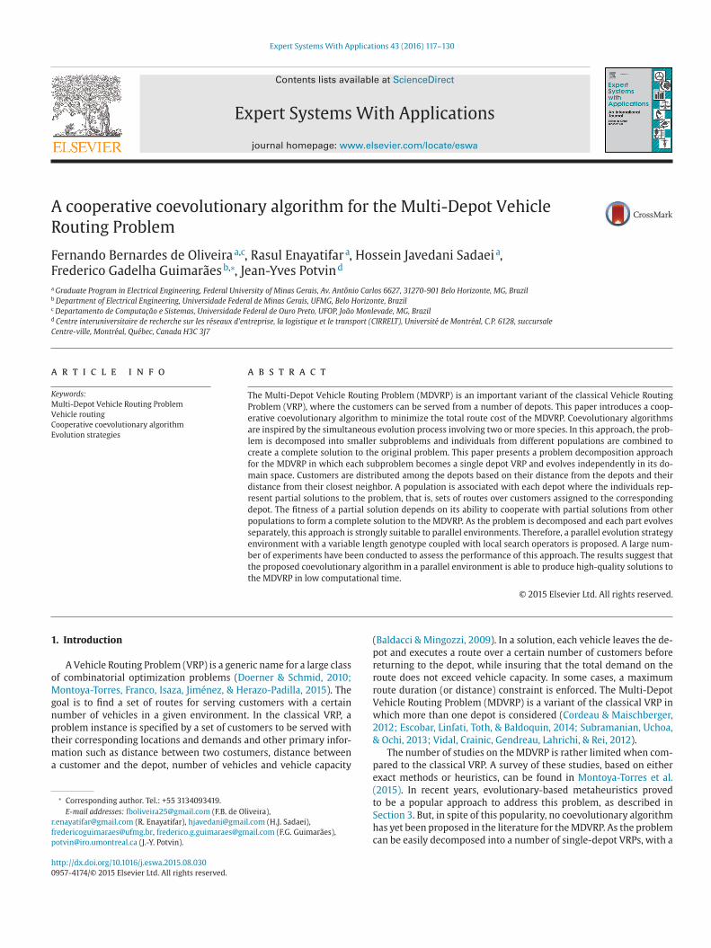
Fig. 1. MDVRP solution.

V

A

s

M

N

N

N

N

N

i

y

x

y

T

g

c

a

C

c

v

h

a

t

2

i

m

s

M

B

C

i

c

a

t

w

(

c

population of partial solutions associated with each depot, a coevolu-

tionary approach looks relevant. Each partial solution or individual in

a population corresponds to vehicle routes defined over the subset of

customers assigned to the corresponding depot. Although each pop-

ulation can evolve separately, this evolution is guided by the ability

of each individual to form good complete solutions with individu-

als from the other populations. This is the problem-solving approach

proposed in this work.

The remainder of this paper is organized as follows. First,

some preliminaries about the MDVRP and coevolution are found in

Section 2. Section 3 presents a literature review. Sections 4 and 5 de-

scribe the proposed methodology while Section 6 reports computa-

tional results. Future avenues for research are proposed in the con-

clusion in Section 7.

2. Preliminaries

In this section, some preliminary information about the mathe-

matical formulation of the MDVRP and cooperative coevolutionary

algorithms are presented.

2.1. Multi-Depot Vehicle Routing Problem formulation

As mentioned earlier, the MDVRP is a variant of the classical VRP

where more than one depot is considered (Montoya-Torres et al.,

2015). Fig. 1 shows a typical solution of this problem with two

depots and two vehicle routes associated with each depot. Typi-

cally, the fleet of vehicles is limited and homogeneous (Cordeau &

Maischberger, 2012; Escobar et al., 2014; Montoya-Torres et al., 2015;

Subramanian et al., 2013; Vidal et al., 2012).

Basically, a solution to this problem is a set of vehicle routes such

that: (i) each vehicle route starts and ends at the same depot, (ii)

each customer is served exactly once by one vehicle, (iii) the to-

tal demand on each route does not exceed vehicle capacity (iv) the

maximum route time is satisfied and (v) the total cost is minimized

(Montoya-Torres et al., 2015).

The MDVRP can be formalized as follows. Let G = (V, A) be a com-

plete graph, where V is the set of nodes and A is the set of arcs. The

nodes are partitioned into two subsets: the customers to be served,

C = {1, . . . , N}, and the multiple depots VD = {N + 1, . . . , N + M},with VC ∪ VD = V and VC ∩ VD = �. There is a non-negative cost cij as-

sociated with each arc (i, j) ∈ A. The demand of each customer is di

(there is no demand at the depot nodes). There is also a fleet of K

identical vehicles, each with capacity Q. The service time at each cus-

tomer i is ti while the maximum route duration time is set to T. A

conversion factor wij might be needed to transform the cost cij into

time units. In this work, however, the cost is the same as the time

and distance units, so wi j = 1.

In the mathematical formulation that follows, binary variables xijk

are equal to 1 when vehicle k visits node j immediately after node i.

uxiliary variables yi are also used in the subtour elimination con-

traints.

inimize

N+M∑

i=1

N+M∑

j=1

K∑

k=1

ci jxi jk , (1)

subject to:

+M∑

i=1

K∑

k=1

xi jk = 1 ( j = 1, . . . , N); (2)

+M∑

j=1

K∑

k=1

xi jk = 1 (i = 1, . . . , N); (3)

+M∑

i=1

xihk −N+M∑

j=1

xh jk = 0 (k = 1, . . . , K; h = 1, . . . , N + M); (4)

+M∑

i=1

N+M∑

j=1

dixi jk ≤ Q (k = 1, . . . , K); (5)

+M∑

i=1

N+M∑

j=1

(ci jwi j + ti

)xi jk ≤ T (k = 1, . . . , K); (6)

N+M∑

=N+1

N∑

j=1

xi jk ≤ 1 (k = 1, . . . , K); (7)

N+M∑

j=N+1

N∑

i=1

xi jk ≤ 1 (k = 1, . . . , K); (8)

i − yj + (M + N)xi jk ≤ N + M − 1;for 1 ≤ i �= j ≤ N and 1 ≤ k ≤ K; (9)

i jk ∈ {0, 1} ∀ i, j, k; (10)

i ∈ {0, 1} ∀ i; (11)

he objective (1) minimizes the total cost. Constraints (2) and (3)

uarantee that each customer is served by exactly one vehicle. Flow

onservation is guaranteed through constraint (4). Vehicle capacity

nd route duration constraints are found in (5) and (6), respectively.

onstraints (7) and (8) check vehicle availability. Subtour elimination

onstraints are in (9). Finally, (10) and (11) define x and y as binary

ariables.

In the original formulation of the MDVRP, a fixed number of ve-

icles is allocated to each depot. In our work, though, the search is

llowed to consider a larger number of vehicles (at a penalty cost in

he objective). This is discussed in Section 5.

.2. Coevolutionary algorithms

Coevolutionary algorithms are a class of evolutionary algorithms

nspired by the simultaneous evolution process involving two or

ore species. Recently, various engineering problems have been

olved with this approach (Blecic, Cecchini, & Trunfio, 2014; Chen,

ori, & Matsuba, 2014; Ladjici & Boudour, 2011; Ladjici, Tiguercha, &

oudour, 2014; Wang & Chen, 2013a; Wang, Cheng, & Huang, 2014).

oevolutionary algorithms are categorized into two groups depend-

ng on the type of interaction among the species, which can be either

ompetitive or cooperative. Competitive coevolution can be viewed as

n arms race, that is, individuals in the populations compete among

hemselves. One group attempts to take advantage over another,

hich responds with an adaptive strategy to recover the advantage

Katada & Handa, 2010). A biological example is the predator–prey

ompetitive coevolution, in which the evolution of one population

F.B. de Oliveira et al. / Expert Systems With Applications 43 (2016) 117–130 119

Fig. 2. Cooperative coevolutionary algorithm with problem decomposition.

a

v

a

I

fi

m

o

a

E

s

A

f

p

i

a

c

i

l

t

n

m

a

l

d

o

f

t

t

i

s

e

e

m

t

2

e

L

3

t

f

S

q

3

k

s

p

i

h

T

l

o

A

c

M

P

h

i

a

u

G

a

C

u

a

t

h

n

t

2

Y

s

I

d

i

E

n

h

t

d

ffects the evolution of the other. This approach has been used in

irtual and simulated evolution (Ebner, 2006) and also for evolving

gent behaviors or artificial players for games (Engelbrecht, 2007).

n cooperative coevolution, the interaction among species is bene-

cial for all or, at least, does not cause any damage. The species

ay live together in the same area and one population needs the

ther ones to survive and evolve. Typically, species cooperate to

ttain a global benefit. This is the case in symbiosis, for example

ngelbrecht (2007).

In a cooperative coevolutionary algorithm, each population repre-

ents a part of a complex decomposable problem (Engelbrecht, 2007).

ccordingly, the true fitness of an individual can only be obtained

rom its interaction with other individuals from the same or other

opulations. Each individual receives a reward or punishment, be-

ng rewarded when it interacts well with the others while getting

punishment otherwise. A cooperative coevolutionary algorithm is

onsidered in this work because the problem can be decomposed

nto smaller subproblems, each one evolving in parallel. Partial so-

utions for those subproblems cooperate to create a complete solu-

ion for the MDVRP. In this situation, a competitive strategy would

ot be suitable because a complete solution is obtained from infor-

ation gathered from all subproblems and there is no competition

mong these subproblems. Fig. 2 depicts a general cooperative coevo-

utionary algorithm with decomposition. A complex problem is first

ecomposed into smaller subproblems. Each population is evolved

n its subproblem and, after a number of generations, individuals

rom these populations are combined to create complete solutions to

he original problem. Through this process, it is possible to compute

he fitness of these complete solutions. Some feedback information

s then returned to each population, such as the best solution found

o far, any required updates to the individuals in the population,

tc.

Coevolutionary algorithms can be distinguished from traditional

volutionary algorithms by their evaluation process (Ficici, 2004). As

entioned above, individuals can only be evaluated through interac-

ion with other individuals from the same or different populations.

Fitness sampling (Engelbrecht, 2007) or fitness assessment (Luke,

013) defines how individuals are combined for the purpose of fitness

valuation. These methods are the followings (Engelbrecht, 2007;

uke, 2013):

(a) All versus all. All possible combinations of individuals from all

populations are considered. This method is very expensive and

can be appropriate for populations with only a few individuals.

(b) Random. Individuals are randomly selected from the coevolv-

ing populations. This method is less expensive than the previ-

ous one and the number of evaluations is typically a parameter

of the method.

(c) All versus best. All individuals of one population are combined

with the best individuals from other populations. This is re-

peated for each population.

(d) Tournament sampling. This process consists of selecting in-

dividuals from each population based on their fitness. Then, a

tournament is performed among all selected individuals to de-

termine a winner. This is typically used in competitive models.

(e) Shared sampling. Only individuals with higher shared fitness

are combined to favor individuals that are significantly differ-

ent from the others in a population.

. Literature review

The literature review focuses on the main issues addressed in

his work. First, Section 3.1 introduces evolutionary-based algorithms

or the MDVRP, followed by parallel algorithms for the MDVRP in

ection 3.2. Then, Section 3.3 is devoted to known applications of se-

uential and parallel coevolutionary algorithms.

.1. Heuristics for the Multi-Depot Vehicle Routing Problem

Evolutionary algorithms (EAs) use a set of candidate solutions,

nown as a population, and heuristic mechanisms to evolve it like

election and reproduction (also called genetic operators). Evolution

roceeds from one generation to the next until a stopping condition

s satisfied (Engelbrecht, 2007; Luke, 2013). Evolutionary algorithms

ave been widely used to solve the VRP, as surveyed in Potvin (2009).

he main contributions with regard to the MDVRP are reported be-

ow.

Genetic algorithms (GAs) are probably the most widely used class

f evolutionary algorithms and were applied as well to the MDVRP.

comprehensive survey of different types of GAs for the MDVRP

an be found in Karakatic and Podgorelec (2015), while GAs for the

DVRP, among other VRP variants, are also described in Gendreau,

otvin, Bräumlaysy, Hasle, and Løkketangen (2008). With regard to

ybrids, a simulated annealing-based solution acceptance criterion

s applied after reproduction in Chen and Xu (2008). The Clarke

nd Wright savings heuristic and the nearest neighbor heuristic are

sed in Ho, Ho, Ji, and Lau (2008) to create initial solutions for the

As. A combination of simulated annealing, bee colony optimization

nd GA is also proposed in Liu (2013). Vidal et al. (2012) and Vidal,

rainic, Gendreau, and Prins (2014) introduce a powerful hybrid GA

sing neighborhood-based heuristics and population-diversity man-

gement schemes to address many different types of VRPs, including

he MDVRP.

Particle swarm optimization (PSO) is inspired by the social be-

avior of agents, such as swarms and birds flock. Individuals are

amed particles, flying in the search space according to simple rules

hat combine local and global information (Engelbrecht, 2007; Luke,

013). This problem-solving methodology was used in Wenjing and

e (2010) for solving the MDVRP.

In addition to EAs, some noteworthy heuristics were proposed to

olve the MDVRP. Tabu Search (TS) has been used in several contexts.

n particular, Renaud, Laporte, and Boctor (1996) and Cordeau, Gen-

reau, and Laporte (1997) use this heuristic for some VRP problems

ncluding MDVRP. A hybrid granular TS algorithm was proposed by

scobar et al. (2014). Those authors introduce the idea of granular

eighborhoods, in which the search process uses restricted neighbor-

oods for each customer defined by a granularity threshold value.

An adaptive large neighborhood search (ALNS) approach was in-

roduced by Pisinger and Ropke (2007). It was applied to solve five

ifferent variants of the VRP, including the MDVRP.

120 F.B. de Oliveira et al. / Expert Systems With Applications 43 (2016) 117–130

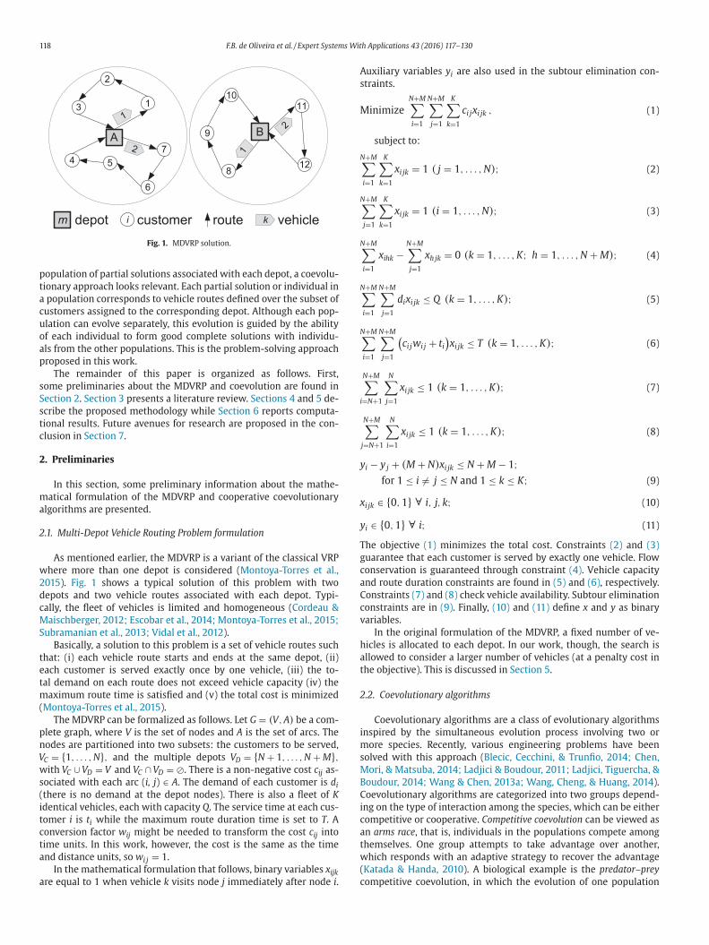
Fig. 3. Problem decomposition: assignment of customers to depots.

4

i

m

s

s

d

a

c

o

t

e

t

T

p

r

i

t

h

(

1

e

i

t

d

c

t

k

t

w

p

p

d

p

The method developed by Subramanian et al. (2013) combines an

exact procedure based on the set partitioning formulation with an

Iterated Local Search (ILS). A Mixed Integer Programming solver is

used for the exact procedure.

3.2. Parallel algorithms for the Multi-Depot Vehicle Routing Problem

A few parallel algorithms for the MDVRP are reported in the lit-

erature. A parallel version of Ant Colony Optimization (ACO) is in-

troduced in Yu, Yang, and Xie (2011). In this work, the MDVRP was

simplified through the definition of a single virtual depot, while in-

suring that the capacity constraint of each vehicle is satisfied. The

algorithm was implemented using a distributed coarse-grained en-

vironment composed of eight computers each equipped with a Pen-

tium processor (3 GHz with 512 MB RAM).

A parallel iterated Tabu Search (TS) is proposed in Maischberger

and Cordeau (2011) and Cordeau and Maischberger (2012). In the first

paper, some preliminary results are reported on eight classes of VRPs

including the MDVRP. The algorithm was run on a cluster made of 128

nodes (each with a 3 GHz Xeon processor). The second paper reports

results over four VRP variants, including the MDVRP, as well as other

variants with time windows.

3.3. Coevolutionary algorithms

In this section, we review different applications of CAs. Note that a

discussion about sequential and parallel versions of CAs can be found

in Popovici and De Jong (2006). The authors show in particular how

different population update strategies can impact the overall perfor-

mance. The authors empirically demonstrate the superiority of the

parallel version over the sequential one on benchmark functions, us-

ing a number of different metrics.

A competitive model with three populations is used in Li,

Guimarães, and Lowther (2015) to solve constrained design problems.

The first population is made of candidate solutions from the design

space while the other populations represent disturbances due to un-

certainties. Li and Yao (2012) propose a cooperative coevolutionary

algorithm in a particle swarm environment. They apply it to large

scale optimization problems on functions with up to 2000 variables.

Other methodologies using particle swarm and coevolution can also

be found in Aote, Raghuwanshi, and Malik (2015) and Chen, Zhu, and

Hu (2010).

A study on sequential and parallel versions of a cooperative

coevolutionary algorithms based on the ES(1+1) evolution strat-

egy is presented in Jansen and Wiegand (2003) 2004). The au-

thors identify situations where a cooperative scheme could be

inappropriate, like problems involving non separable functions.

Depending on the decomposition method or the characteris-

tics of the function, the coevolutionary algorithm could even be

harmful.

As far as we know, the coevolutionary paradigm has never been

applied to the MDVRP. With regard to vehicle routing in general, a

large scale capacitated arc routing problem is addressed in Mei, Li,

and Yao (2014) using a coevolutionary algorithm. In this work, the

routes are grouped into different subsets to be optimized and prob-

lem instances with more than 300 edges are solved. A multi-objective

capacitated arc routing problem is also studied in Shang et al. (2014).

A coevolutionary algorithm is presented in Wang and Chen (2013b)

for a pickup and delivery problem with time windows. To minimize

the number of vehicles and the total traveling distance, the authors

use two populations: one for diversification purposes and the other

for intensification purposes. In the scheduling domain, a competi-

tive coevolutionary quantum genetic algorithm for minimizing the

makespan of a job shop scheduling problem is reported in Gu, Gu,

Cao, and Gu (2010).

. Cooperative coevolutionary model for the MDVRP

A cooperative coevolutionary model with problem decomposition

s proposed here to solve the MDVRP. The main contribution of this

ethod is the computational efficiency resulting from the decompo-

ition of the problem into subproblems. Each subproblem becomes a

ingle depot VRP and evolves independently in its domain space. The

ecomposition approach considers the depots separately and assigns

subset of customers to each one. Some overlap is possible, that is,

ustomers might be associated with one or more depots depending

n their neighbors (other customers or depots). An evolving popula-

ion is associated with each subproblem and the (partial) solutions in

ach population must then cooperate to form a complete solution to

he MDVRP. In this section, we explain the decomposition approach.

hen, Section 5 describes the evolution process for solving the sub-

roblems.

Each customer is assigned to a depot using the two following

ules:

1. The closest depot.

2. The closest depot to the closest neighbor node (if different

from the one in rule 1).

When the two rules identify the same depot, the assignment

s obvious. When the two rules identify two different depots, then

he conflict must be addressed in some way. Fig. 3 illustrates

ow these rules are applied. In the figure, there are three depots

nodes A–C) and 20 customers (nodes 1–20). For customer 1, rule

identifies A as the closest depot. Then, rule 2 identifies the clos-

st neighbor to customer 1 as customer 2, whose closest depot

s also A. Thus, customer 1 can only be assigned to depot A. In

he figure, all white nodes can only be assigned to their closest

epot.

Now, let us consider customer 6. Rule 1 identifies B as the

losest depot. Then, rule 2 identifies the closest neighbor to cus-

omer 6 as customer 7, whose closest depot is A. Since we do not

now if it is better to assign customer 6 to depot A or B, cus-

omer 6 is initially assigned to both depots. That is, this customer

ill be part of the two evolving populations associated with de-

ots A and B. It implies that there is some overlap among the sub-

roblems. In Fig. 3, all gray nodes are assigned to two different

epots.

The assignment procedure is further detailed in Algorithm 1 . The

rocedure starts with the set of customers V , the set of depots V ,

C D

F.B. de Oliveira et al. / Expert Systems With Applications 43 (2016) 117–130 121

Algorithm 1: Assignment of customers.

1 assignCustomers(VC,VD, A)

2 for i ← 1 to N do // for each customer i

// Rule 1: closest depot3 mi ← getClosestDepot(VD, i);

4 insert(Ami, i);

// Rule 2: depot of the closest neighbor5 j ← getClosestNeighbor(VC, i);

6 m j ← getClosestDepot(VD, j);

7 if (mi �= m j) then // Different depots8 insert(Am j

, i);

9 end if

10 end for

11 return(A1 . . . AM);

12 end

Fig. 4. Cooperative coevolutionary model for the MDVRP.

a

t

m

t

i

p

i

A

(

c

t

p

p

a

a

o

o

t

e

M

i

t

s

b

a

c

p

o

e

l

p

Algorithm 2: CoES —general scheme.

1 CoES(VC,VD, A, N, M, Q))

2 A1 . . . AM ← assignCustomers(VC,VD, A);

3 [P1 . . . PM] ← initializePopulations(A1 . . . AM,μ,α);

4 S ← createCompleteSolutions(P1 . . . PM);

5 f ← evaluateSolutions(S);

6 s∗ ← getBestSolution();

7 startModules();

8 return(s∗);

9 end

Fig. 5. Giant tour representation and the obtained routes.

5

p

e

G

a

s

l

o

a

a

b

E

e

T

t

t

t

2

l

a

i

b

s

i

i

S

5

w

c

v

o

a

t

b

a

t

e

s well as the set of arcs A. In Line 3 the closest depot mi to cus-

omer i is selected according to rule 1 and inserted in the assign-

ent group Amiof depot mi (Line 4). The closest neighbor to cus-

omer i is defined as customer j (Line 5) and the closest depot to j,

dentified as mj, is selected according to rule 2. The depots are com-

ared in Line 7. If the two depots are different (mi �= mj), customer

is also inserted in the allocation group Am jof depot mj (Line 8).

fter processing all customers, the assignment groups are returned

Line 11).

After this decomposition, each subproblem becomes a classi-

al single depot VRP for a subset of customers identified by the

wo assignment rules above. Given that the gray nodes are du-

licated, a repair operator will be needed to obtain a valid com-

lete solution (see Section 5.5). Each subproblem is solved with

n evolutionary algorithm, in which each individual represents

partial solution to the MDVRP. Fig. 4 illustrates the structure

f the proposed coevolutionary model. For each depot, there is

ne population which evolves and searches the best routes for

he set of customers assigned to it. Then, one individual for

ach population is selected to create a complete solution for the

DVRP.

A decomposition approach is particularly interesting for problem

nstances with a low degree of interdependency (coupling) between

he subproblems. For example, customer 19 in Fig. 3 should clearly be

erved by depot C. It is unlikely that good solutions will be obtained

y assigning this customer to depots A or B, and these solutions are

utomatically eliminated through the decomposition approach. It is

lear that some degree of interdependency exists among the sub-

roblems for the instance illustrated in Fig. 3, due to the presence

f gray nodes.

This model is strongly suitable for a parallel environment where

ach population evolves separately and cooperates with other popu-

ations to solve the problem. A parallel architecture for this model is

roposed in the next section.

. Parallel evolution strategy

A parallel environment exploiting the evolution strategy (ES)

aradigm, called CoES, supports the evolution of our cooperative co-

volutionary model. Evolution strategy (Engelbrecht, 2007; Freitas,

uimarães, Pedrosa Silva, & Souza, 2014; Luke, 2013) is an evolution-

ry algorithm using mutation as the main operator to generate new

olutions. ES was chosen because each subproblem has a variable

ength representation (genotype) and the design of a recombination

perator in this case would be rather cumbersome (see Section 5.2).

The proposed parallelization scheme, which is operational under

synchronous updates, is shown in Algorithm 2. CoES first receives

ll required information about the problem, in particular the num-

er of customers (N), number of depots (M) and vehicle capacity (Q).

ach population is initialized with μ individuals (Line 3), which are

ncoded using the representation scheme presented in Section 5.1.

he initialization procedure uses a semi-greedy method to insert cus-

omers from a given list. Parameter α defines the number of cus-

omers in this list, as discussed in Section 5.2. Complete solutions are

hen created with a Random fitness sampling strategy (Engelbrecht,

007) (Line 4). Here, individuals from each initial population are se-

ected randomly to create complete solutions. It should be noted that

nother strategy is used in the following populations, as explained

n Section 5.5. In Line 5, all complete solutions are evaluated and the

est one is selected (Line 6). Then, a number of parallel modules are

tarted (Line 7). At the end, the best complete solution to the MDVRP

s returned (Line 8).

The representation and initialization procedures are described

n Sections 5.1 and 5.2. The parallel modules are introduced in

ection 5.3.

.1. Representation

Individuals from each population are represented by a giant tour,

ithout route delimiters. It is basically a single sequence made of all

ustomers assigned to a depot, as shown in Fig. 5(a). Since each indi-

idual in a population corresponds to a particular depot and subset

f customers, the length of the giant tour is likely to change (vari-

ble genotype). Individual routes are created from this giant tour with

he Split algorithm (Prins, 2004), which can optimally extract feasi-

le routes from a single sequence. In constrained problems, the Split

lgorithm can be relaxed at the beginning to allow infeasible routes

hat violate one or more constraints. During the execution of the co-

volutionary algorithm, this relaxation is progressively reduced to

122 F.B. de Oliveira et al. / Expert Systems With Applications 43 (2016) 117–130

Algorithm 3: Populations initialization.

1 initializePopulations(A1 . . . AM,μ,α)

2 for i ← 1 to M do

3 for j ← 1 to μ do

4 if ( j == 1) then // Greedy construction5 ind j ← greedy(Ai);

6 else // Semi-Greedy construction7 ind j ← semiGreedy(Ai, α);

8 end if

9 end for

10 insert(Pi, ind j);

11 end for

12 end

Fig. 6. Architecture of the parallel modules in CoES.

Algorithm 4: Start Modules.

1 startModules()

2 start ← FALSE;

3 createThread(Monitor());

4 createThread(PE());

5 createThread(CSE());

6 createThread(EG());

7 start ← TRUE;

8 end

Fig. 7. Population Evolve module.

p

u

E

u

l

c

s

t

p

5

t

l

t

λd

s

p

i

t

t

converge toward feasible routes. Fig. 5(b) illustrates two routes that

could be obtained from the giant tour representation in 5(a).

5.2. Initialization

The population initialization procedure is shown in Algorithm 3 .

The first individual in each population is constructed with the Nearest

Insertion Heuristic (NIH) (Bodin, Golden, Assad, & Ball, 1983) while

the other ones are constructed with a semi-greedy approach based

on NIH. With regard to the first individual, the closest customer to

the depot is first inserted in the giant tour. Then, the next customer

to be inserted is the one which is closest to the previous one. This is

repeated until the giant tour is complete.

Based on this greedy heuristic, a semi-greedy variant generates

the remaining individuals. The first customer is selected at random.

Then, the remaining customers are sorted based on their distance

from the previous one. A restricted candidate list (RCL) is created with

the α best-ranked customers and the next customer to be inserted is

selected at random in the RCL. This is repeated until the giant tour is

complete.

5.3. Parallel modules and coordination

The parallel modules are executed until a stopping criterion, based

on the execution time, is met. Fig. 6 depicts the architecture of these

modules within CoES as well as their communication scheme.

The Start Modules procedure is shown in Algorithm 4 . It is called

in Line 7 of Algorithm 2 to create a thread for each module and to

initialize the environment. A start flag is used to indicate that each

module should wait until all modules have been initialized. At the

beginning of the procedure, the flag is set to FALSE (Line 2). At the

end, the start flag is set to TRUE (Line 7) so that all modules can be

executed.

The Monitor module manages the parallel processes and transmits

information about the MDVRP problem. When the time-based stop-

ing criterion is met, all modules are terminated by the Monitor mod-

le and the best solution is returned.

The Population Evolve (PE) module evolves each population with

S. The Complete Solutions Evaluate (CSE) module combines individ-

als from different populations to create and evaluate complete so-

utions. In addition, it applies local search heuristics to improve the

omplete solutions. The Elite Group (EG) module maintains an elite

et of complete solutions, and also applies local search heuristics to

hese elite solutions. The various modules mentioned above are ex-

lained in detail in the following sections.

.4. Population Evolve (PE) module

The Population Evolve (PE) module manages the ES-based evolu-

ion by creating a thread for each population. Within a thread, the evo-

ution process is run sequentially. This is represented in Fig. 7. Note

hat the ES-based evolution is highlighted in the gray box of Fig. 7.

With regard to the ES-based population evolution, each one of the

offspring is generated as follows. First, a parent is selected at ran-

om, so that each parent generates λ/μ offspring on average. The

elf-adaptive procedure updates the number of mutations (strategy

arameter σ ) using a binomial distribution B(n, p). The distribution

s computed with n equal to the number of customers in the giant

our (genotype length) and p equal to 0.5. The mutation is applied

o the giant tour by selecting two different random positions and

F.B. de Oliveira et al. / Expert Systems With Applications 43 (2016) 117–130 123

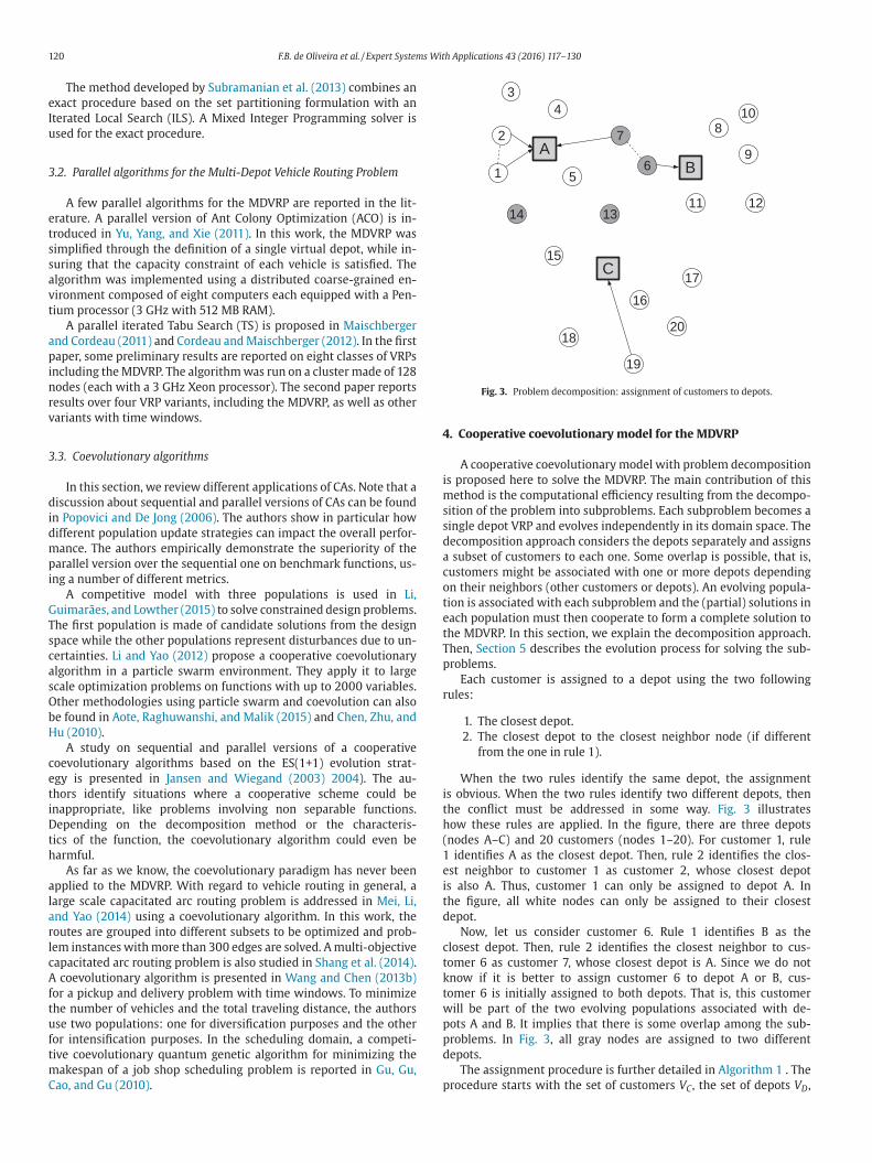
Fig. 8. Complete Solutions Evaluate module.

b

T

t

n

t

w

i

f

i

a

t

b

r

e

t

l

i

s

o

a

d

s

W

t

(

c

p

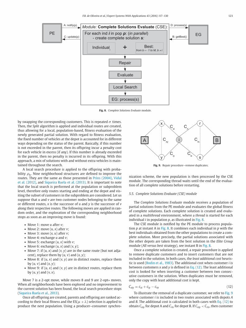
Fig. 9. Repair procedure—remove duplicates.

n

m

t

5

p

o

a

i

t

b

p

t

m

t

i

t

b

c

u

o

C

w

a

o

y swapping the corresponding customers. This is repeated σ times.

hen, the Split algorithm is applied and individual routes are created,

hus allowing for a local, population-based, fitness evaluation of the

ewly generated partial solution. With regard to fitness evaluation,

he fixed number of vehicles at the depot is accounted for in different

ays depending on the status of the parent. Basically, if this number

s not exceeded in the parent, then its offspring incur a penalty cost

or each vehicle in excess (if any). If this number is already exceeded

n the parent, then no penalty is incurred in its offspring. With this

pproach, a mix of solutions with and without extra vehicles is main-

ained throughout the search.

A local search procedure is applied to the offspring with proba-

ility ρls. Nine neighborhood structures are defined to improve the

outes. They are the same as those presented in Prins (2004), Vidal

t al. (2012), and Siqueira Ruela et al. (2013). It is important to note

hat the local search is performed at the population or subproblem

evel, therefore only routes starting and ending at the depot and vis-

ting the subset of customers in the subproblem are considered. Let us

uppose that u and v are two customer nodes belonging to the same

r different routes, x is the successor of u and y is the successor of v

long their respective routes. The following moves are applied in ran-

om order, and the exploration of the corresponding neighborhood

tops as soon as an improving move is found:

• Move 1: move u after v;• Move 2: move (u, x) after v;• Move 3: move (x, u) after v;• Move 4: exchange u and v;• Move 5: exchange (u, x) with v;• Move 6: exchange (u, x) and (v, y);• Move 7: if (u, x) and (v, y) are in the same route (but not adja-

cent), replace them by (u, v) and (x, y);• Move 8: if (u, x) and (v, y) are in distinct routes, replace them

by (u, v) and (x, y);• Move 9: if (u, x) and (v, y) are in distinct routes, replace them

by (u, y) and (v, x).

Move 7 is a 2-opt move, while moves 8 and 9 are 2-opt∗ moves.

hen all neighborhoods have been explored and no improvement to

he current solution has been found, the local search procedure stops

Siqueira Ruela et al., 2013).

Once all offspring are created, parents and offspring are ranked ac-

ording to their local fitness and the ES(μ + λ) selection is applied to

roduce the next population. Using a producer–consumer synchro-

ization scheme, the new population is then processed by the CSE

odule. The corresponding thread waits until the end of the evalua-

ion of all complete solutions before restarting.

.5. Complete Solutions Evaluate (CSE) module

The Complete Solutions Evaluate module receives a population of

artial solutions from the PE module and evaluates the global fitness

f complete solutions. Each complete solution is created and evalu-

ted in a multithread environment, where a thread is started for each

ndividual i in population p, as illustrated in Fig. 8.

The CSE module is notified by the PE module to process popula-

ion p at instant A in Fig. 8. It combines each individual in p with the

est individuals obtained from the other populations to create a com-

lete solution. More precisely, the partial solutions associated with

he other depots are taken from the best solution in the Elite Group

odule (All versus best strategy), see instant B in Fig. 8.

Once a complete solution is created, a repair procedure is applied

o remove duplicate customers and to insert customers that are not

ncluded in the solution. In both cases, the least additional cost heuris-

ic is used (Bodin et al., 1983). The additional cost when customer i is

etween customers x and y is defined in Eq. (12). The least additional

ost is looked for when inserting a customer between two consec-

tive customers in the solution. When duplicates must be removed,

nly the copy with least additional cost is kept.

xiy = cxi + ciy − cxy (12)

To illustrate the removal of a duplicate customer, we refer to Fig. 9

here customer i is included in two routes associated with depots A

nd B. The additional cost is calculated in both cases with Eq. (12) to

btain Cxiy for depot A and Cris for depot B. If Cxiy < Cris, then customer

124 F.B. de Oliveira et al. / Expert Systems With Applications 43 (2016) 117–130

Fig. 10. Repair procedure—insert customer.

Fig. 11. Elite Group module.

(a) Initial solution

(b) Guiding solution

Fig. 12. Path-Relinking!.

v

f

t

d

r

t

g

t

t

f

c

i

t

i

t

i

b

t

t

6

t

d

e

e

stances are Euclidean and the time units are the same as the distance

1 The MDVRP instances might also be obtained in https://github.com/

fboliveira/MDVRP-Instances .

i is kept in the route of depot A and the duplicate is removed from the

route of depot B.

When inserting a customer in a solution, all insertion positions

between two consecutive customers are considered and the least cost

one is chosen. In Fig. 10, customer i is inserted between customers x

and y in a route of depot A.

The complete solution is evaluated and submitted to a local search

procedure with probability ρls. The local search is based on the same

moves than those presented in Section 5.4. However, it is now pos-

sible for a customer to be moved from one depot to another, thus

changing individuals in the populations. This is the reason for the

population update at instant C in Fig. 8. After the update, the PE mod-

ule is notified and can restart.

Each complete solution created is sent to the EG module at instant

D in Fig. 8. The module checks if the complete solution can be part of

the elite group, as it is explained next.

5.6. Elite Group (EG) module

The Elite Group (EG) module maintains a set of τ elite complete

solutions, including the best solution to the MDVRP found so far. This

is illustrated in Fig. 11. Assuming that a complete solution is submit-

ted by the CSE module, the EG module will try to add the solution to

the elite group. If there are less than τ solutions in the elite group,

the solution is automatically added. Otherwise, the new solution can

enter the elite group only if it is better than the worst solution in the

group, in which case it replaces the latter.

The local search for the elite group operates in two steps, called

PR and RI, where PR stands for Path Relinking and RI for Route Im-

provement. The local search is run in a multithread environment with

a thread for each solution in the elite group.

PR uses each solution in the elite group as an initial solution and

the best solution so far as the guiding solution. To apply PR in this

setting, the difference between an initial solution i and the guiding

solution g must be calculated. We assume that each customer in a

solution is characterized by the vehicle serving this customer and the

corresponding depot. For each customer, the triplet (customer, depot,

ehicle) from the guiding solution is added to set � when it differs

rom the initial solution.

We refer to Fig. 12 for an example. In this figure, we have one ini-

ial solution (Fig. 12a) and a guiding solution (Fig. 12b). There are two

epots A and B, 12 customers and two vehicles at each depot (rep-

esented by the pentagons numbered 1 and 2). The difference be-

ween the initial and guiding solutions corresponds to the nodes in

ray, namely customers 2 and 11. Thus � = {(2, B, 2), (11, A, 1)}. The

riplets in � are then processed one by one to progressively modify

he initial solution. That is, the customer in the first triplet is removed

rom its route in the initial solution and reinserted in the route indi-

ated by the depot and vehicle of the guiding solution. A new solution

s obtained which is closer to the guiding solution. The procedure is

hen applied again using the new solution and the second triplet. This

s repeated until all triplets are done. It is hoped that a solution bet-

er than the guiding solution will emerge along the path between the

nitial and guiding solutions.

The RI improvement procedure is applied to the solution returned

y PR. This procedure is the local search mentioned in Section 5.5. If

he solution obtained at the end is better than the best solution, then

he elite group is updated.

. Computational results

The performance of the proposed CoES algorithm was assessed

hrough a number of computational experiments. They were con-

ucted on the 33 MDVRP benchmark instances taken from the lit-

rature (Cordeau et al., 1997; Cordeau & Maischberger, 2012; Escobar

t al., 2014; Subramanian et al., 2013; Vidal et al., 2012).1 These in-

F.B. de Oliveira et al. / Expert Systems With Applications 43 (2016) 117–130 125

Table 1

Selected parameter values.

Parameter Lower bound Upper bound

Tmax 600 s 1800 s

Tupd 300 s 600 s

μ 20 100

τ 5 50

ρls 0.2 0.8

u

h

w

c

u

i

p

6

p

p

μt

p

ρ

f

t

T

f

t

e

t

a

o

c

p

a

t

s

T

v

i

(

a

A

b

s

fi

s

s

a

t

e

p

Table 2

Significant factors and interac-

tions.

Factor/interaction p-value

μ < 2−16

τ 0.035

μ:ρls:τ 0.016

Table 3

Final parameter values.

Parameter Value

Tmax 1800 s

Tupd 600 s

μ 20

τ 50

ρls 0.2

20 100

0

2

4

6

8

Number of individuals

10 50

0

2

4

6

8

Elite group size

Fig. 13. Boxplots of the two main factors.

20.5

0.0.

2

20.5

0.0.

8

0

1

2

3

4

5

6

7

Interaction with Pls rate

20.5

0.0.

2.60

0.30

0

20.5

0.0.

2.18

00.3

00

20.5

0.0.

2.60

0.60

0

20.5

0.0.

2.18

00.6

00

0

1

2

3

4

5

6

7

Interaction with Tmax and Tupd

Fig. 14. Boxplots of interactions.

o

t

B

a

p

r

nits. They are divided into S1 (P01 − P23) and S2 (P24 − P33)2 and

ave various sizes ranging from 48 to 360 customers, see Table 4.

The algorithm was implemented in C++ 113 and all experiments

ere run on a computer with two 2.50 GHz Intel Xeon (E5-2640) pro-

essors with 12 cores per CPU and 96 GB RAM. The computer was run

nder the Ubuntu 14.04.1 LTS operational system.

A first experiment was realized to set the parameter values, as it

s discussed in Section 6.1. A comparison with the best solutions re-

orted in the literature follows in Section 6.2.

.1. Parameter settings

The algorithm stops when it reaches either the allowed total com-

utation time Tmax or the maximum computation time without im-

rovement to the best solution Tupd. Also, the number of individuals

in each population and the maximum number of complete solu-

ions in the elite group τ must be defined. Finally, the local search

rocedure in the PE and CSE modules are applied with a probability

ls.

After some preliminary tests and using some values commonly

ound in the literature, lower and upper bound values were de-

ermined for the above parameters. These values are presented in

able 1.

As there are two values (levels) for each parameter (factors), a 2k

actorial experiment was designed to study the impact of each fac-

or as well as their interactions. There are five factors with two lev-

ls each, resulting in 32 observations (25) for each instance. Selecting

he instance in group S1 (P01 − P23) from the benchmark, we obtain

total of 736 observations (i.e., 32 × 23). Given the large number

f factors and total observations, an experiment with a single repli-

ation was performed. In this situation, the Sparsity-of-effects princi-

le applies, that is, the main effects and low-order interactions usu-

lly dominate. Then, we can use an experiment with one replica-

ion and combine highest-order interaction for calculating the mean

quare error (Campelo, 2015, Chap. 12; Montgomery & Runger, 2011),

he response variable corresponds to the gap between the solution

alue obtained by CoES and the best-known solution value reported

n Vidal et al. (2012).

The experiment is performed with the analysis of variance

ANOVA) method from the R-Project (Core Team, 2015). Among other

ssumptions, ANOVA requires a normal distribution for the residuals.

s the number of samples is large, they are approximately normal

ecause of the Central Limit Theorem (CLT) and this assumption is

atisfied.

Table 2 reports only the significant factors and interactions identi-

ed by ANOVA. In this case, the null hypothesis states that there is no

ignificant impact and a p-value smaller than 0.05 invalidates this as-

umption. Table 2 shows the significant factors identified by ANOVA

long with their corresponding p-value.

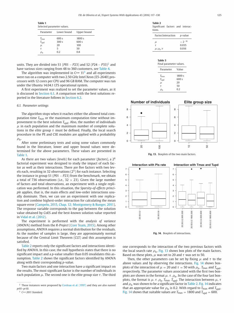
Two main factors and one interaction have a significant impact on

he results. The most significant factor is the number of individuals in

ach population μ. The second one is the elite group size τ . The third

2 Those instances were proposed by Cordeau et al. (1997) and they are also named

r01–pr10.3 C++ 2011 Standard.

p

p

a

t

F

ne corresponds to the interaction of the two previous factors with

he local search rate ρls. Fig. 13 shows box plots of the main factors.

ased on these plots, μ was set to 20 and τ was set to 50.

Then, the other parameters can be set by fixing μ and τ to the

bove values and by observing the interactions. Fig. 14 shows box-

lots of the interaction of μ = 20 and τ = 50 with ρls, Tmax and Tupd,

espectively. The parameter values associated with the first two box-

lots are shown in the format μ. τ. ρls. In the case of the four last box-

lots, the format is μ. τ. ρls. Tmax .Tupd. The interaction between μ, τnd ρls was shown to be a significant factor in Table 2. Fig. 14 indicates

hat an appropriate value for ρls is 0.2. With regard to Tmax and Tupd,

ig. 14 shows that suitable values are Tmax = 1800 and Tupd = 600.

126 F.B. de Oliveira et al. / Expert Systems With Applications 43 (2016) 117–130

Table 4

CoES(λ = μ): results.

Inst M N Q T Average values Best cost

Time (s) Cost

P01 4 50 80 ∞ 1.00 (*) 576.87 576.87

P02 2 50 160 ∞ 0.50 475.06 473.87

P03 3 75 140 ∞ 2.50 643.57 641.19

P04 8 100 100 ∞ 189.70 1011.42 1007.40

P05 5 100 200 ∞ 26.60 752.39 750.11

P06 6 100 100 ∞ 77.30 877.86 876.50

P07 4 100 100 ∞ 24.20 893.36 888.41

P08 14 249 500 310 803.40 4474.23 4450.37

P09 12 249 500 310 513.30 3904.92 3895.70

P10 8 249 500 310 719.90 3680.02 3666.35

P11 6 249 500 310 396.20 3593.37 3569.68

P12 5 80 60 ∞ 0.90 (*) 1318.95 1318.95

P13 5 80 60 200 0.00 (*) 1318.95 1318.95

P14 5 80 60 180 0.00 (*) 1360.12 1360.12

P15 5 160 60 ∞ 107.00 2549.65 2526.06

P16 5 160 60 200 8.20 (*) 2572.23 2572.23

P17 5 160 60 180 14.70 2733.80 2709.09

P18 5 240 60 ∞ 429.10 3781.66 3771.35

P19 5 240 60 200 72.60 (*) 3827.06 3827.06

P20 5 240 60 180 190.20 4094.86 4058.07

P21 5 360 60 ∞ 554.90 5668.97 5608.26

P22 5 360 60 200 214.00 5708.78 5702.16

P23 5 360 60 180 529.30 6159.90 6129.99

P24 1 48 200 500 0.00 849.17 849.17

P25 2 96 195 480 630.80 1271.39 1269.56

P26 3 144 190 460 123.60 1768.13 1759.77

P27 4 192 185 440 580.80 2057.50 2041.76

P28 5 240 180 420 321.00 2362.75 2314.72

P29 6 288 175 400 724.40 2690.01 2674.53

P30 1 72 200 500 0.60 (*) 1070.85 1070.85

P31 2 144 190 475 254.00 1650.96 1633.34

P32 3 216 180 450 652.50 2160.76 2139.78

P33 4 288 170 425 472.80 2844.32 2825.90

Average 261.70 2445.57 2432.67

S1 211.98 2694.69 2682.55

S2 376.05 1872.58 1857.94

Table 5

CoES(λ = μ): comparison with results of the literature—best values.

Instance CGL ITS ILS-RVND-SP HGSADC+ ELTG

P01 0.00 0.00 0.00 0.00 0.00

P02 0.00 0.07 0.07 0.07 0.07

P03 −0.61 0.00 0.00 0.08 0.00

P04 0.07 0.64 0.64 0.82 0.64

P05 −0.43 0.01 0.01 0.01 0.01

P06 −0.15 0.00 0.00 0.00 0.00

P07 −0.40 0.73 0.73 0.73 0.42

P08 −0.72 1.41 1.62 1.77 1.80

P09 −0.64 0.90 0.94 0.96 0.38

P10 −1.30 0.97 0.96 0.97 1.01

P11 −0.31 0.62 0.67 0.67 0.69

P12 0.00 0.00 0.00 0.00 0.00

P13 0.00 0.00 0.00 0.00 0.00

P14 0.00 0.00 0.00 0.00 0.00

P15 −0.32 0.82 0.82 0.82 0.82

P16 0.00 0.00 0.00 0.00 0.00

P17 −0.41 0.00 0.00 0.00 0.00

P18 1.64 1.85 1.85 1.85 1.85

P19 0.00 0.00 0.00 0.00 0.00

P20 0.00 0.00 0.00 0.00 0.00

P21 1.31 2.44 2.44 2.44 2.44

P22 −0.24 0.00 0.00 0.00 0.00

P23 −0.16 0.84 0.84 0.84 0.57

P24 −1.41 −1.41 −1.41 −1.41 −1.41

P25 −3.45 −2.89 −2.89 −2.89 −3.17

P26 −3.08 −2.44 −2.44 −2.44 −2.44

P27 −2.51 −0.80 −0.80 −0.85 −1.08

P28 −3.88 −0.71 −0.71 −1.09 −1.49

P29 −3.38 −0.12 −0.23 −0.28 −1.32

P30 −1.95 −1.72 −1.72 −1.72 −1.72

P31 −2.56 −1.89 −1.89 −1.90 −1.93

P32 −1.70 0.31 0.31 0.26 −0.54

P33 −8.54 −1.82 −1.68 −2.10 −2.92

Average −1.06 −0.07 −0.06 −0.07 −0.22

S1 −0.12 0.49 0.50 0.52 0.47

S2 −3.25 −1.35 −1.35 −1.44 −1.80

s

u

o

b

1

w

t

i

e

o

d

o

i

t

W

T

w

a

m

T

w

e

s

S

C

b

The final parameter settings for the CoES algorithm are summa-

rized in Table 3. The comparison with other algorithms in the next

section is based on these parameter values.

6.2. Comparison with other methods

The performance of our CoES was compared with the best heuris-

tics proposed for the MDVRP, namely, the Tabu Search (CGL) (Cordeau

et al., 1997), the adaptive large neighborhood search (ALNS) (Pisinger

& Ropke, 2007), a fuzzy logic guided genetic algorithm (FLGA) (Lau,

Chan, Tsui, & Pang, 2010), a parallel iterated Tabu Search heuris-

tic (ITS) (Cordeau & Maischberger, 2012), a hybrid algorithm com-

bining Iterated Local Search and Set Partitioning (ILS-RVND-SP)

(Subramanian et al., 2013), a hybrid genetic algorithm with adaptive

diversity control (HGSADC+) (Vidal et al., 2014) and a hybrid Granular

Tabu Search (ELTG) (Escobar et al., 2014).

CoES was run 10 times on all benchmark instances, using the pre-

viously defined parameter settings. To remove any factor that could

impact the performance, the order of execution of all replicates was

randomized. Note that heuristics CGL and ELTG were run only once

on each instance and the value reported was used to compare with

the best value of CoES.

The results from CoES are shown in Table 4. The instance name is

in column Inst, M is the number of depots, N is the number of cus-

tomers, Q is the vehicle capacity and T is the maximum duration time

of a vehicle route (∞ means that there is no time constraint). The

next two columns present the average values for the processing time

(in seconds) and for the solution cost. When (∗) appears, the same

olution was produced by CoES in each of the 10 runs. The last col-

mn shows the best solution cost obtained by CoES.

The best and mean solution values, when compared with the

ther methods, are shown in Tables 5 and 6, respectively. These ta-

les report the gap (in %), that is,

00 × (ZCoES − Zlit)

Zlit

here ZCoES is the solution value of CoEs and Zlit the value of one of

he other methods (as reported in the literature). A negative value

ndicates that CoES performs better. The Average line reports the av-

rage gap over all instances. The lines S1 and S2 show the average gap

ver the instances in each subset. In the tables, the entries in bold in-

icate that the same or better solution values were obtained by CoES

ver the corresponding method.

With regard to the solutions reported in Table 4 labeled with (∗),

t should be noted that the gap with the other methods in Table 6 for

hose instances is always null (gap = 0.00) or negative (gap < 0.00).

hen considering the gap between CoES and the other methods in

able 6 for the mean values, the average over all test instances is al-

ays smaller than 0.5%. It is less than 0.9% for subset S1, while it is

lways negative for S2, indicating that CoES provides an improve-

ent over each method in this case. When considering the gap in

able 5 for the best values, the average over all test instances is al-

ays negative. It indicates that CoES provides an improvement over

very method. The trend observed for the mean values is also ob-

erved here: there is generally a positive gap in the case of subset

1, but a more important negative gap for S2. Thus, we conclude that

oES performs better on subset S2.

As HGSADC+ uses an evolutionary approach, some analyses have

een performed using average costs and time for that method as a

F.B. de Oliveira et al. / Expert Systems With Applications 43 (2016) 117–130 127

Table 6

CoES(λ = μ): comparison with results of the literature—mean values.

Instance CGL ALNS FLGA ITS ILS-RVND-SP HGSADC+ ELTG

P01 0.00 0.00 0.00 0.00 0.00 0.00 0.00

P02 0.25 0.32 0.32 0.32 0.32 0.32 0.32

P03 −0.25 0.37 0.37 0.37 0.37 0.46 0.37

P04 0.47 0.53 0.98 1.01 1.04 1.08 1.04

P05 −0.13 0.01 0.04 0.31 0.29 0.31 0.31

P06 0.00 −0.58 −0.55 0.16 0.16 0.16 0.16

P07 0.16 0.45 0.61 1.29 1.29 1.29 0.98

P08 −0.18 1.20 0.81 1.60 1.83 2.07 2.35

P09 −0.41 0.32 −0.29 0.92 1.05 1.14 0.62

P10 −0.93 0.36 0.28 1.17 1.25 1.33 1.39

P11 0.35 0.56 0.32 1.27 1.33 1.30 1.36

P12 0.00 −0.01 0.00 0.00 0.00 0.00 0.00

P13 0.00 0.00 0.00 0.00 0.00 0.00 0.00

P14 0.00 0.00 0.00 0.00 0.00 0.00 0.00

P15 0.61 1.19 1.42 1.77 1.77 1.77 1.77

P16 0.00 −0.07 −0.24 0.00 0.00 0.00 0.00

P17 0.50 0.91 0.91 0.91 0.87 0.91 0.91

P18 1.92 1.21 1.43 2.13 2.13 2.13 2.13

P19 0.00 −0.30 −0.35 0.00 −0.01 0.00 0.00

P20 0.91 0.74 0.78 0.91 0.91 0.91 0.91

P21 2.40 3.04 2.59 3.55 3.55 3.55 3.55

P22 −0.13 −0.23 −0.42 0.12 0.05 0.12 0.12

P23 0.33 1.10 1.00 1.33 1.33 1.31 1.06

P24 −1.41 −1.41 −1.41 −1.41 −1.41 −1.41 −1.41

P25 −3.32 −2.75 −3.16 −2.75 −2.84 −2.75 −3.03

P26 −2.62 −2.10 −2.30 −2.00 −1.99 −1.98 −1.98

P27 −1.75 −0.17 −0.90 −0.17 −0.17 −0.04 −0.32

P28 −1.88 1.07 −1.20 1.09 1.05 1.35 0.56

P29 −2.82 0.09 −1.43 0.26 0.18 0.51 −0.75

P30 −1.95 −1.72 −1.72 −1.72 −1.72 −1.72 −1.72

P31 −1.51 −0.83 −0.94 −0.87 −0.85 −0.83 −0.87

P32 −0.74 1.14 0.40 1.02 1.19 1.29 0.43

P33 −7.94 −1.57 −2.58 −1.47 −1.32 −0.83 −2.28

Average −0.61 0.09 −0.16 0.34 0.35 0.42 0.24

S1 0.26 0.48 0.44 0.83 0.85 0.88 0.84

S2 −2.59 −0.83 −1.52 −0.80 −0.79 −0.64 −1.14

Fig. 15. Average gap based on the ratio between customers and depots.

r

s

b

s

e

e

i

a

t

I

t

a

i

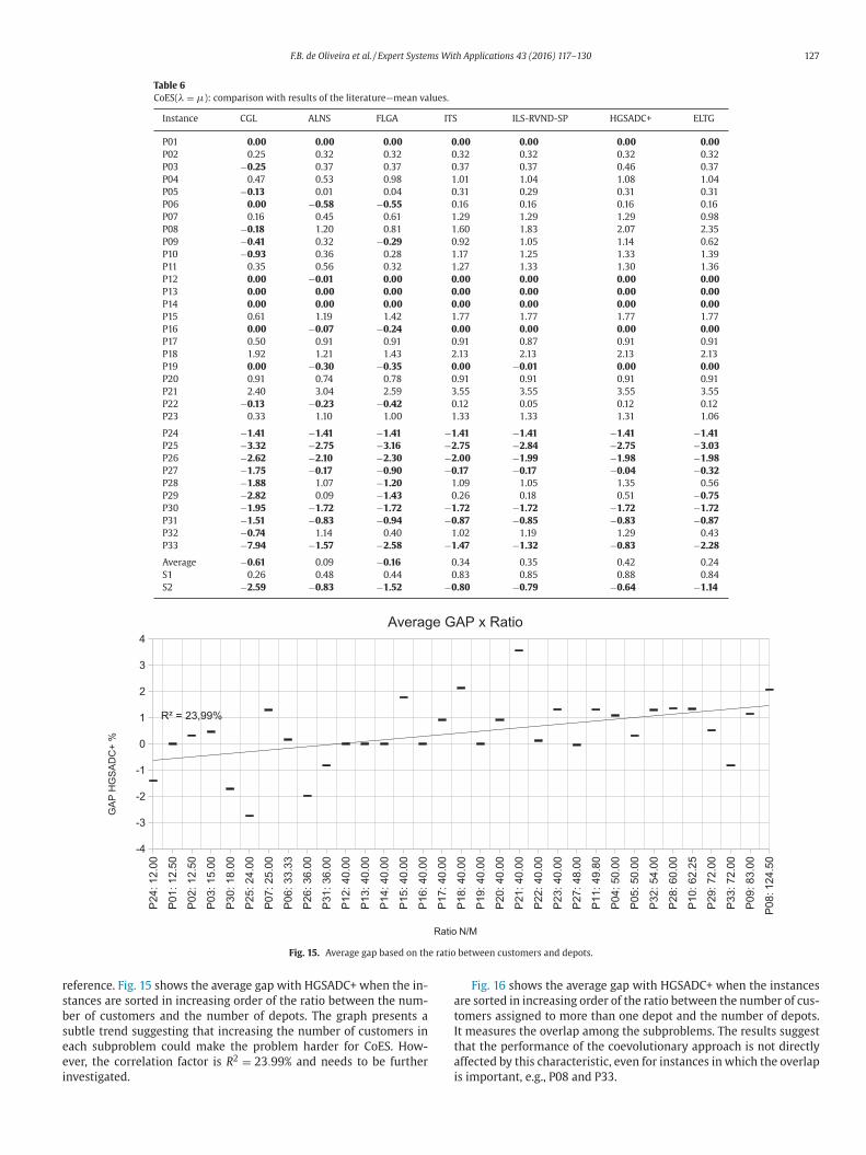
eference. Fig. 15 shows the average gap with HGSADC+ when the in-

tances are sorted in increasing order of the ratio between the num-

er of customers and the number of depots. The graph presents a

ubtle trend suggesting that increasing the number of customers in

ach subproblem could make the problem harder for CoES. How-

ver, the correlation factor is R2 = 23.99% and needs to be further

nvestigated.

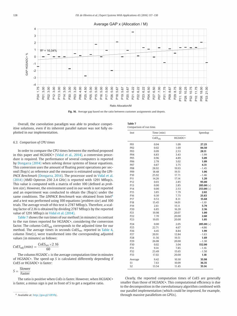
Fig. 16 shows the average gap with HGSADC+ when the instances

re sorted in increasing order of the ratio between the number of cus-

omers assigned to more than one depot and the number of depots.

t measures the overlap among the subproblems. The results suggest

hat the performance of the coevolutionary approach is not directly

ffected by this characteristic, even for instances in which the overlap

s important, e.g., P08 and P33.

128 F.B. de Oliveira et al. / Expert Systems With Applications 43 (2016) 117–130

Fig. 16. Average gap based on the ratio between customer assignments and depots.

C

Table 7

Comparison of run time.

Inst Time (min) Speedup

CoESadj HGSADC+

P01 0.04 1.09 27.25

P02 0.02 1.69 84.50

P03 0.09 2.53 28.11

P04 6.83 3.43 −1.99

P05 0.96 4.89 5.09

P06 2.78 3.02 1.09

P07 0.87 3.75 4.31

P08 28.92 19.93 −1.45

P09 18.48 19.51 1.06

P10 25.92 17.71 −1.46

P11 14.26 17.14 1.20

P12 0.03 2.85 95.00

P13 0.00 2.85 285.00 (∗)

P14 0.00 2.53 253.00 (∗)

P15 3.85 7.79 2.02

P16 0.30 7.75 25.83

P17 0.53 8.31 15.68

P18 15.45 14.01 −1.10

P19 2.61 15.11 5.79

P20 6.85 16.20 2.36

P21 19.98 20.07 1.00

P22 7.70 20.00 2.60

P23 19.05 20.00 1.05

P24 0.00 2.05 205.00 (∗)

P25 22.71 4.67 −4.86

P26 4.45 8.84 1.99

P27 20.91 12.84 −1.63

P28 11.56 19.51 1.69

P29 26.08 20.00 −1.30

P30 0.02 3.04 152.00

P31 9.14 7.85 −1.16

P32 23.49 15.65 −1.50

P33 17.02 20.00 1.18

Average 9.42 10.50 35.98

S1 7.63 10.09 36.35

S2 13.54 11.45 35.14

s

Overall, the coevolution paradigm was able to produce compet-

itive solutions, even if its inherent parallel nature was not fully ex-

ploited in our implementation.

6.3. Comparison of CPU times

In order to compare the CPU times between the method proposed

in this paper and HGSADC+ (Vidal et al., 2014), a conversion proce-

dure is required. The performance of several computers is reported

by Dongarra (2014) when solving dense systems of linear equations.

This conversion uses the amount of floating point operations per sec-

ond (flop/s) as reference and the measure is estimated using the LIN-

PACK Benchmark (Dongarra, 2014). The processor used in Vidal et al.

(2014) (AMD Opteron 250 2.4 GHz) is reported with 1291 Mflop/s.

This value is computed with a matrix of order 100 (defined as prob-

lem size). However, the environment used in our work is not reported

and an experiment was conducted to obtain the (flop/s) under the

same conditions. The LINPACK Benchmark was obtained from Intel4

and a test was performed using 100 equations (problem size) and 100

trials. The average result of this test is 2787 Mflop/s. Therefore, a scal-

ing factor of 2.16 is obtained by dividing 2787 Mflop/s by the reported

value of 1291 Mflop/s in Vidal et al. (2014).

Table 7 shows the run times of our method (in minutes) in contrast

to the run times reported for HGSADC+, considering the conversion

factor. The column CoESadj corresponds to the adjusted time for our

method. The average times in seconds CoESsec reported in Table 4,

column Time(s), were transformed into the corresponding adjusted

values (in minutes) as follows:

oESadj(min) = CoESsec×2.16

60

The column HGSADC+ is the average computation time in minutes

of HGSADC+. The speed-up S is calculated differently depending if

CoES or HGSADC+ is faster:

S = Slower

Faster

The ratio is positive when CoEs is faster. However, when HGSADC+

is faster, a minus sign is put in front of S to get a negative ratio.

4 Available at: http://goo.gl/1ZEYbj .

t

o

t

Clearly, the reported computation times of CoES are generally

maller than those of HGSADC+. This computational efficiency is due

o the decomposition in the coevolutionary algorithm combined with

ur parallel implementation (which could be improved, for example,

hrough massive parallelism on GPUs).

F.B. de Oliveira et al. / Expert Systems With Applications 43 (2016) 117–130 129

7

s

p

l

p

p

p

c

l

H

T

c

t

m

u

d

i

t

s

t

c

m

e

e

e

A

c

t

m

A

F

a

d

p

N

g

g

s

R

A

B

B

B

C

C

C

C

C

C

C

D

D

E

E

E

F

F

G

G

H

J

J

K

K

L

L

L

L

L

L

L

M

. Conclusion and future work

This paper proposed a cooperative coevolutionary algorithm to

olve the MDVRP. In this algorithm, each depot is associated with a

opulation with its assigned customers. Individuals in each popu-

ation represent partial single-depot solutions to the problem. Each

opulation evolves separately, but the quality of an individual de-

ends on its ability to cooperate with partial solutions from other

opulations to form a good complete solution to the MDVRP.

The results show that our coevolutionary algorithm produces

ompetitive solutions when compared with the best known so-

utions, even improving some of them. Besides, it is faster than

GSDAC+, which is the best method reported in the literature.

he benefit of our approach comes from its ability to decompose

omplex problems into simpler subproblems and evolve solutions

o the subproblems in parallel. The decomposition approach also

akes the method more scalable. In large MDVRP instances, it is

nlikely that customers close to a depot will be allocated to a

istant depot. Therefore, the coevolutionary algorithm incorporates

mportant characteristics of a problem instance and allows a reduc-

ion of the search space. Moreover, the evolutionary engine leads to

impler representations and genetic operators. Finally, the coevolu-

ionary algorithm proposed in this work would greatly benefit from

loud computing architectures, cluster computing and GPU program-

ing.

One interesting avenue of research would be to integrate math-

matical programming into the local searches (matheuristic). Since

ach subproblem reduces to a single-depot VRP, the use of math-

matical programming within each population could be beneficial.

dditionally, other sophisticated local search strategies could be in-

orporated into the EG module, like Tabu Search. Finally, we intend

o improve the parallel implementation by exploiting GPU program-

ing for the PE, CSE and EG modules.

cknowledgments

F. B. Oliveira would like to thank the financial support from CAPES

oundation, Ministry of Education of Brazil, grant BEX 0295/14-0, for

warding the scholarship for the visit period at CIRRELT in Université

e Montréal.

R. Enayatifar and H. Javedani Sadaei would like to thank the sup-

ort given by the Brazilian Agency CAPES.

F. G. Guimarães would like to thank the support given by the

ational Council for Scientific and Technological Development (CNPq

rant no. 312276/2013-3), Brazil.

J.-Y. Potvin would like to thank the Natural Sciences and En-

ineering Research Council of Canada (NSERC) for its financial

upport.

eferences

ote, S., Raghuwanshi, M., & Malik, L. (2015). A new particle swarm optimizer with

cooperative coevolution for large scale optimization. In S. C. Satapathy, B. N. Biswal,S. K. Udgata, & J. Mandal (Eds.), Proceedings of the third international conference on

frontiers of intelligent computing: Theory and applications (FICTA) 2014. In Advancesin intelligent systems and computing: vol. 327 (pp. 781–789). Springer International

Publishing. doi:10.1007/978-3-319-11933-5_88.aldacci, R., & Mingozzi, A. (2009). A unified exact method for solving different

classes of vehicle routing problems. Mathematical Programming, 120(2), 347–380.

doi:10.1007/s10107-008-0218-9.lecic, I., Cecchini, A., & Trunfio, G. A. (2014). Fast and accurate optimization of a

GPU-accelerated {CA} urban model through cooperative coevolutionary particleswarms. Procedia Computer Science, 29(0), 1631–1643. 2014 International confer-

ence on computational science http://dx.doi.org/10.1016/j.procs.2014.05.148.odin, L., Golden, B., Assad, A., & Ball, M. (1983). Routing and scheduling of vehicles and

crews: The state of the art. Computers & Operations Research, 10(2), 63–211.

ampelo, F. (2015). Lecture notes on design and analysis of experiments. Version2.11, creative commons BY-NC-SA 4.0. https://github.com/fcampelo/Design-and-

Analysis-of-Experiments.hen, H., Mori, Y., & Matsuba, I. (2014). Solving the balance problem of massively multi-

player online role-playing games using coevolutionary programming. Applied SoftComputing, 18(0), 1–11. http://dx.doi.org/10.1016/j.asoc.2014.01.011.

hen, H., Zhu, Y., & Hu, K. (2010). Discrete and continuous optimization based on multi-swarm coevolution. Natural Computing, 9(3), 659–682. doi:10.1007/s11047-009-

9174-4.

hen, P., & Xu, X. (2008). A hybrid algorithm for multi-depot vehicle routing problem.In IEEE international conference on service operations and logistics, and informatics,

2008. IEEE/SOLI 2008: vol. 2 (pp. 2031–2034). doi:10.1109/SOLI.2008.4682866.ordeau, J.-F., Gendreau, M., & Laporte, G. (1997). A tabu search heuristic for periodic

and multi-depot vehicle routing problems. Networks, 30(2), 105–119.ordeau, J.-F., & Maischberger, M. (2012). A parallel iterated tabu search heuristic

for vehicle routing problems. Computers & Operations Research, 39(9), 2033–2050.

http://dx.doi.org/10.1016/j.cor.2011.09.021.ore TeamR. (2015). R: A language and environment for statistical computing. Vienna,

Austria: R Foundation for Statistical Computing.oerner, K., & Schmid, V. (2010). Survey: Matheuristics for rich vehicle routing prob-

lems. In M. Blesa, C. Blum, G. Raidl, A. Roli, & M. Sampels (Eds.), Hybrid metaheuris-tics. In Lecture notes in computer science: vol. 6373 (pp. 206–221). Berlin, Heidelberg:

Springer. doi:10.1007/978-3-642-16054-7_15.

ongarra, J. J. (2014). Performance of various computers using standard linear equationssoftware (Linpack benchmark report). Technical report, CS-89-85.University of Ten-

nessee Computer Science.bner, M. (2006). Coevolution and the red queen effect shape virtual plants. Genetic

Programming and Evolvable Machines, 7, 103–123. doi:10.1007/s10710-006-7013-2.ngelbrecht, A. (2007). Computational intelligence: An introduction. Wiley.

scobar, J., Linfati, R., Toth, P., & Baldoquin, M. (2014). A hybrid granular tabu search

algorithm for the multi-depot vehicle routing problem. Journal of Heuristics, 20(5),483–509. doi:10.1007/s10732-014-9247-0.

icici, S. G. (2004). Solution concepts in coevolutionary algorithms. Waltham, MA, USA:(Ph.D. thesis). Faculty of Brandeis University.AAI3127125

reitas, A. R. R., Guimarães, F. G., Pedrosa Silva, R. C., & Souza, M. J. F. (2014). Memeticself-adaptive evolution strategies applied to the maximum diversity problem. Op-

timization Letters, 8(2), 705–714. doi:10.1007/s11590-013-0610-0.

endreau, M., Potvin, J.-Y., Bräumlaysy, O., Hasle, G., & Løkketangen, A. (2008). Meta-heuristics for the vehicle routing problem and its extensions: A categorized bibli-

ography. In B. Golden, S. Raghavan, & E. Wasil (Eds.), The vehicle routing problem:Latest advances and new challenges. In Operations research/computer science inter-

faces: vol. 43 (pp. 143–169). US: Springer. doi:10.1007/978-0-387-77778-8_7.u, J., Gu, M., Cao, C., & Gu, X. (2010). A novel competitive co-evolutionary quantum

genetic algorithm for stochastic job shop scheduling problem. Computers & Opera-

tions Research, 37(5), 927–937. Disruption management http://dx.doi.org/10.1016/j.cor.2009.07.002.

o, W., Ho, G. T., Ji, P., & Lau, H. C. (2008). A hybrid genetic algorithm for the multi-depot vehicle routing problem. Engineering Applications of Artificial Intelligence,

21(4), 548–557. http://dx.doi.org/10.1016/j.engappai.2007.06.001.ansen, T., & Wiegand, R. (2003). Sequential versus parallel cooperative coevolutionary

(1+1) EAS. In The 2003 congress on evolutionary computation, 2003. CEC ’03: vol. 1(pp. 30–37). doi:10.1109/CEC.2003.1299553.

ansen, T., & Wiegand, R. P. (2004). The cooperative coevolutionary (1+1) EA. Evolution-

ary Computation, 12(4), 405–434.arakatic, S., & Podgorelec, V. (2015). A survey of genetic algorithms for solving

multi depot vehicle routing problem. Applied Soft Computing, 27(0), 519–532.http://dx.doi.org/10.1016/j.asoc.2014.11.005.

atada, Y., & Handa, Y. (2010). Tracking the red queen effect by estimating features ofcompetitive co-evolutionary fitness landscapes. In 2010 IEEE congress on evolution-

ary computation (CEC) (pp. 1–8). doi:10.1109/CEC.2010.5586188.

adjici, A., & Boudour, M. (2011). Nash–Cournot equilibrium of a deregulated electric-ity market using competitive coevolutionary algorithms. Electric Power Systems Re-

search, 81(4), 958–966. http://dx.doi.org/10.1016/j.epsr.2010.11.016.adjici, A., Tiguercha, A., & Boudour, M. (2014). Nash equilibrium in a two-

settlement electricity market using competitive coevolutionary algorithms.International Journal of Electrical Power & Energy Systems, 57(0), 148–155.

http://dx.doi.org/10.1016/j.ijepes.2013.11.045.

au, H., Chan, T., Tsui, W., & Pang, W. (2010). Application of genetic algorithms to solvethe multidepot vehicle routing problem. IEEE Transactions on Automation Science

and Engineering, 7(2), 383–392. doi:10.1109/TASE.2009.2019265.i, M., Guimarães, F., & Lowther, D. A. (2015). Competitive co-evolutionary algorithm for

constrained robust design. IET Science, Measurement & Technology, 9(2), 218–223.doi:10.1049/iet-smt.2014.0204.

i, X., & Yao, X. (2012). Cooperatively coevolving particle swarms for large scale

optimization. IEEE Transactions on Evolutionary Computation, 16(2), 210–224.doi:10.1109/TEVC.2011.2112662.

iu, C.-Y. (2013). An improved adaptive genetic algorithm for the multi-depot vehiclerouting problem with time window. Journal of Networks, 8(5), 1035–1042.

uke, S. (2013). Essentials of metaheuristics (2nd). Lulu. Available for free athttp://cs.gmu.edu/˜sean/book/metaheuristics/

aischberger, M., & Cordeau, J.-F. (2011). Solving variants of the vehicle routing prob-

lem with a simple parallel iterated tabu search. In J. Pahl, T. Reiners, & S. Voß (Eds.),Network optimization. In Lecture notes in computer science: vol. 6701 (pp. 395–400).

Berlin and Heidelberg: Springer. doi:10.1007/978-3-642-21527-8_44.

130 F.B. de Oliveira et al. / Expert Systems With Applications 43 (2016) 117–130

S

V

V

W

W

W

W

Y

Mei, Y., Li, X., & Yao, X. (2014). Cooperative coevolution with route distance groupingfor large-scale capacitated arc routing problems. IEEE Transactions on Evolutionary

Computation, 18(3), 435–449. doi:10.1109/TEVC.2013.2281503.Montgomery, D., & Runger, G. (2011). Applied statistics and probability for engineers

(5th). John Wiley & Sons.Montoya-Torres, J. R., Franco, J. L., Isaza, S. N., Jiménez, H. F., & Herazo-

Padilla, N. (2015). A literature review on the vehicle routing problem with mul-tiple depots. Computers & Industrial Engineering, 79(0), 115–129. http://dx.doi.org/

10.1016/j.cie.2014.10.029.

Pisinger, D., & Ropke, S. (2007). A general heuristic for vehicle routing prob-lems. Computers & Operations Research, 34(8), 2403–2435. http://dx.doi.org/

10.1016/j.cor.2005.09.012.Popovici, E., & De Jong, K. (2006). Sequential versus parallel cooperative coevolutionary

algorithms for optimization. In IEEE congress on evolutionary computation, 2006.CEC 2006 (pp. 1610–1617). doi:10.1109/CEC.2006.1688501.

Potvin, J.-Y. (2009). State-of-the art review-evolutionary algorithms for vehicle routing.

INFORMS Journal on Computing, 21(4), 518–548. doi:10.1287/ijoc.1080.0312.Prins, C. (2004). A simple and effective evolutionary algorithm for the vehi-

cle routing problem. Computers & Operations Research, 31(12), 1985–2002.http://dx.doi.org/10.1016/S0305-0548(03)00158-8.

Renaud, J., Laporte, G., & Boctor, F. F. (1996). A tabu search heuristic for the multi-depot vehicle routing problem. Computers & Operations Research, 23(3), 229–235.

http://dx.doi.org/10.1016/0305-0548(95)O0026-P.

Shang, R., Wang, Y., Wang, J., Jiao, L., Wang, S., & Qi, L. (2014). A multi-populationcooperative coevolutionary algorithm for multi-objective capacitated arc rout-

ing problem. Information Sciences, 277, 609–642. http://dx.doi.org/10.1016/j.ins.2014.03.008.

Siqueira Ruela, A., Gadelha Guimaraes, F., Rabelo Oliveira, R., Neves, B., PeixotoAmorim, V., & Fraga, L. (2013). A parallel hybrid genetic algorithm on cloud com-

puting for the vehicle routing problem with time windows. In 2013 IEEE in-

ternational conference on systems, man, and cybernetics (SMC) (pp. 2467–2472).doi:10.1109/SMC.2013.421.

ubramanian, A., Uchoa, E., & Ochi, L. S. (2013). A hybrid algorithm for a class ofvehicle routing problems. Computers & Operations Research, 40(10), 2519–2531.

http://dx.doi.org/10.1016/j.cor.2013.01.013.idal, T., Crainic, T. G., Gendreau, M., Lahrichi, N., & Rei, W. (2012). A hybrid genetic al-

gorithm for multidepot and periodic vehicle routing problems. Operations Research,60(3), 611–624. doi:10.1287/opre.1120.1048.

idal, T., Crainic, T. G., Gendreau, M., & Prins, C. (2014). Implicit depot assignmentsand rotations in vehicle routing heuristics. European Journal of Operational Research,

237(1), 15–28. http://dx.doi.org/10.1016/j.ejor.2013.12.044.

ang, H.-F., & Chen, Y.-Y. (2013a). A coevolutionary algorithm for the flexible deliveryand pickup problem with time windows. International Journal of Production Eco-

nomics, 141(1), 4–13. Meta-heuristics for manufacturing scheduling and logisticsproblems http://dx.doi.org/10.1016/j.ijpe.2012.04.011.

ang, H.-F., & Chen, Y.-Y. (2013b). A coevolutionary algorithm for the flexible deliveryand pickup problem with time windows. International Journal of Production Eco-

nomics, 141(1), 4–13. Meta-heuristics for manufacturing scheduling and logistics

problems http://dx.doi.org/10.1016/j.ijpe.2012.04.011.ang, X., Cheng, H., & Huang, M. (2014). QoS multicast routing protocol oriented

to cognitive network using competitive coevolutionary algorithm. Expert Systemswith Applications, 41(10), 4513–4528. http://dx.doi.org/10.1016/j.eswa.2014.01.

020.enjing, Z., & Ye, J. (2010). An improved particle swarm optimization for the multi-

depot vehicle routing problem. In 2010 International conference on E-business and

e-government (ICEE) (pp. 3188–3192). doi:10.1109/ICEE.2010.803.u, B., Yang, Z. Z., & Xie, J.-X. (2011). A parallel improved ant colony optimization for

multi-depot vehicle routing problem. Journal of the Operational Research Society,62(1), 183–188.