A Coordination-Based Algorithm for Dedicated Destination Vehicle Routing inB2B E-Commerce

Tsung-Yin Ou1, Chen-Yang Cheng2, Chun Hsiung Lai3 and Hsin-Pin Fu1,*

1Department of Marketing and Distribution Management, National Kaohsiung University of Science and Technology, Taiwan2Department of Industrial Engineering and Management, Taipei University of Technology, Taiwan3Department of Enterprise Information and Industrial Engineering, Tunghai University, Taiwan

�Corresponding Author: Hsin-Pin Fu. Email: hpfu@nkust.edu.twReceived: 09 March 2021; Accepted: 09 May 2021

Abstract: This paper proposes a solution to the open vehicle routing problem withtime windows (OVRPTW) considering third-party logistics (3PL). For the typicalOVRPTW problem, most researchers consider time windows, capacity, routinglimitations, vehicle destination, etc. Most researchers who previously investigatedthis problem assumed the vehicle would not return to the depot, but did not con-sider its final destination. However, by considering 3PL in the B2B e-commerce,the vehicle is required back to the nearest 3PL location with available space. Thispaper formulates the problem as a mixed integer linear programming (MILP)model with the objective of minimizing the total travel distance. A coordinaterepresentation particle swarm optimization (CRPSO) algorithm is developed toobtain the best delivery sequencing and the capacity of each vehicle. Results ofthe computational study show that the proposed method provides solution withina reasonable amount of time. Finally, the result compared to PSO also indicatesthat the CRPSO is effective.

Keywords: Third-party logistics; open vehicle routing problem with timewindows; dedicated destination

Notationst: Iteration index, t = 1…Ti: Particle index, i = 1…Id: Dimension index, d = 1…Du: Uniform random number in the interval [0,1]w(t): Inertia weight in the tth iterationvid(t): Velocity of the ith particle at the dth dimension in the tth iterationxid(t): Position of the ith particle at the dth dimension in the tth iterationPid: Personal best position (pbest) of the ith particle in the dth dimensionPgd: Global best position (gbest) in the dth dimensionCp: Personal best position acceleration constantCg: Global best position acceleration constantXmax: Maximum position value

This work is licensed under a Creative Commons Attribution 4.0 International License, whichpermits unrestricted use, distribution, and reproduction in any medium, provided the originalwork is properly cited.

Computer Systems Science & EngineeringDOI:10.32604/csse.2022.018432

Article

echT PressScience

Xmin: Minimum position valueXi: Vector position of the ith particle, [xi1, xi2, … xiD]Vi: Vector velocity of the ith particle, [vi1, vi2, … viD]Pi: Vector personal best position of the ith particle, [Pi1, Pi2, … PiD]Pg: Vector global best position, [Pg1, Pg2, … PgD]Ri: Set of vehicle routes corresponding to the ith particleDi: Set of distances between vehicles and destinations corresponding to ith particleΨ(Xi): Fitness value of Xi

1 Introduction

In B2B e-commerce, logistics is viewed as an increasingly important activity. Regardless of industry,most e-businesses rely on logistics management to enhance their competitiveness [1]. Despite theimportance of logistics management, e-businesses tend to focus primarily on developing their coreabilities (e.g., R&D, product, marketing). Logistics and other non-core activities often are outsourced toother companies [2]. Independent third-party logistics (3PL) companies provide professional, integrateddistribution services and information technology to help decrease fixed and variable costs of logistics [3].With the rapid development of electronic commerce, e-businesses are facing new challenges in thelogistics supply chain and are partnering extensively with 3PL firms to deliver products on time, increasecustomer satisfaction, decrease logistics costs and increase profits.

Logistics professionals must take many constraints into account in order to plan optimal distributionroutes that consider customer demand, vehicle routing, vehicle capacity, etc. Together, these constraintsassociated with delivery logistics are called the vehicle routing problem (VRP) [4]. Ref. [5] solved onlinepick-to-sort order batching problem for managing frequent arrivals in B2B e-commerce. Ref. [6] appliedthe meta-heuristic method of ant colony optimization (ACO) to an established set of vehicle routingproblems (VRP). The VRP can be divided into two types: the Hamiltonian cycle (traditional VRP, wherethe vehicle returns to the depot), and the Hamiltonian path (the open vehicle routing problem, or OVRP,where the vehicle does not need to return to the depot). Thus, routing destination is the biggest differencebetween the VRP and the OVRP.

In this paper, we propose a solution to the open vehicle routing problem with time windows (OVRPTW)considering 3PL. In the problem, a 3PL company leaves its vehicles at its client’s depot until they are loaded.Post-delivery, vehicles do not return to the depot, but to the nearest 3PL company location with availablespace. In most previous OVRPTW literature that considered 3PL, a vehicle’s final destination was notconsidered. However, in this research, we not only consider common constraints in OVRPTW such asvehicle capacity, but also a 3PL constraint in which the vehicles must return to a 3PL company location ·a limitation of destination. We propose a mixed integer linear programming (MILP) model that considersthese practical characteristics. In this research, we use a classical OVRPTW formulation with 3PLconsiderations to solve an experimental problem set. Due to the computational complexity of the model,we designed a coordinate representation particle swarm optimization (CRPSO) algorithm to obtain thenear-optimal vehicle routing plan with the objective of minimizing total travel distance.

The rest of this paper is organized as follows. In Section 2, we review the literature on related VRPsconsidering 3PL and OVRPTW. In Section 3, we present the proposed MILP model for the problem andthe CRPSO algorithm used to obtain the solutions. In Section 4, we present a computational study thatdemonstrates the excellent performance of the CRPSO algorithm. Finally, in Section 5 we summarize theresults of this research and suggest a possible direction for future research.

896 CSSE, 2022, vol.40, no.3

2 Literature Review

Many enterprises outsource non-core functions such as distribution logistics to promotecompetitiveness; in response to this trend, the 3PL sector is growing rapidly [2]. Increasingly, VRPresearchers also are considering 3PL. [7] presented a web-based decision support system (DSS) for wastelube oils collection and recycling operations considering cooperation with a 3PL company. Because thelogistics function is outsourced to a 3PL company, vehicle routing begins from the depot and ends at a3PL location. This feature of delivery is similar to our research. In the study, the DSS system enablesschedulers to tackle reverse supply chain management problems interactively and can be applied torealistic reverse logistical planning problems [8].

Baykasoglu and Kaplanoglu proposed a multi-agent based load consolidation decision-makingapproach considering many kinds of logistics mechanisms, including in-house logistics systems and 3PL,so as to improve the logistics efficiency of enterprises [9]. Amorim et al. formulated models for a case ofperishable goods with a mix of fixed and loose shelf lives. When the shelf life of product did not matchthe distribution plan, it would be outsourced to a 3PL company. The results show that the economicbenefits derived from using an integrated approach depend greatly on the freshness level of deliveredproducts [10]. Moon et al. extended the VRPTW to the VRPTW with overtime and outsourcing vehicles(VRPTWOV), which allows overtime for drivers and the possibility of using outsourced vehicles. Theydeveloped a mixed integer programming model, a genetic algorithm (GA) and a hybrid algorithm basedon simulated annealing to demonstrate the efficiency of their solution [11]. In this paper, we extendresearch in this important area by proposing a solution to an experimental problem set that incorporates3PL considerations into a classical OVRPTW formulation.

Routing destination is the biggest difference between VRP and OVRP. VRP is called the Hamiltoniancycle, and OVRP is called the Hamiltonian path [12]. All other constraints, such as vehicle capacity, timewindows, etc. are the same. OVRP was not as important as VRP in the early 1980s. Schrage was the firstto classify routing types and define OVRP with the objective of minimizing the number of routes(i.e., vehicles) and total cost [13].

OVRP is a very common problem in daily life, especially in logistics, transportation and other similarindustries. Several scholars have proposed solutions to problems in these contexts. Sariklis and Powellproposed a two-stage model based on a minimum spanning tree to solve a vehicle routing decisionproblem [14]. Li et al. developed a hybrid ant colony algorithm (ACO) combined with taboo search (TA)to solve OVRP [15]. Fleszar et al. proposed variable neighborhood search (VNS) to determine thecustomer service sequence [16]. OVRPTW (the focus of this research) extends OVRP by considering theconcept of time windows. Recently, researchers have proposed solutions to such problems. Repoussiset al. proposed a comprehensive mathematical model to capture all aspects of OVRPTW, which theysolved using a greedy look-ahead route construction heuristic algorithm [7].

In most of the extant literature, researchers solved VRP, VRPTW, OVRP and OVRPTW as individualproblems. Unlike previous studies, however, this paper addresses a new topic: OVRPTW considering 3PL.Since OVRPTW is NP-hard, most researchers have solved such problems using heuristic algorithms [16].However, due to the computational complexity of the model, it was necessary to develop an algorithmbased on particle swarm optimization (PSO) to solve the proposed problem. Since a standard PSOalgorithm cannot be applied to discrete problems directly, the encoding and decoding methods are critical.Ai and Kachitvichyanukul proposed a PSO algorithm for solving a vehicle routing problem withsimultaneous pickup and delivery (VRPSPD) as well as a capacitated vehicle routing problem (CVRP)[17,18]. The solution representation for VRPSPD with n customers and m vehicles is a (n + 2m)dimensional particle. The decoding method starts by transforming the particle into a priority list ofcustomers and a priority matrix of vehicles to serve each customer. The vehicle routes are constructed

CSSE, 2022, vol.40, no.3 897

based on the customer priority list and the vehicle priority matrix. Applying this encoding method, wepropose a coordinate representation particle swarm optimization (CRPSO) algorithm to obtain the optimalsolution. The designed algorithm with n customers and m vehicles yields (n + 2m + m) dimensions foreach particle. The encoding and decoding methods are described in detail in Section 4.

3 OVRPTW Considering 3PL

3.1 Problem Description

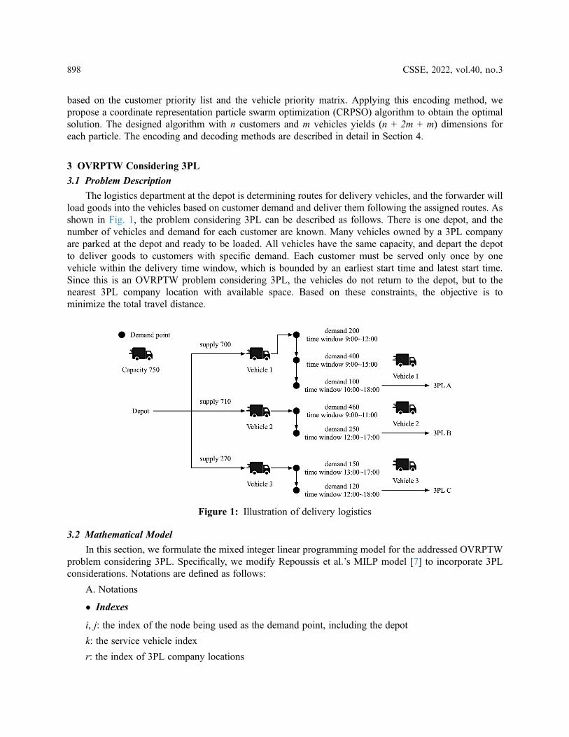
The logistics department at the depot is determining routes for delivery vehicles, and the forwarder willload goods into the vehicles based on customer demand and deliver them following the assigned routes. Asshown in Fig. 1, the problem considering 3PL can be described as follows. There is one depot, and thenumber of vehicles and demand for each customer are known. Many vehicles owned by a 3PL companyare parked at the depot and ready to be loaded. All vehicles have the same capacity, and depart the depotto deliver goods to customers with specific demand. Each customer must be served only once by onevehicle within the delivery time window, which is bounded by an earliest start time and latest start time.Since this is an OVRPTW problem considering 3PL, the vehicles do not return to the depot, but to thenearest 3PL company location with available space. Based on these constraints, the objective is tominimize the total travel distance.

3.2 Mathematical Model

In this section, we formulate the mixed integer linear programming model for the addressed OVRPTWproblem considering 3PL. Specifically, we modify Repoussis et al.’s MILP model [7] to incorporate 3PLconsiderations. Notations are defined as follows:

A. Notations

� Indexes

i, j: the index of the node being used as the demand point, including the depot

k: the service vehicle index

r: the index of 3PL company locations

Figure 1: Illustration of delivery logistics

898 CSSE, 2022, vol.40, no.3

� Sets

N: the set of customers including node of the depot, where i or j = 1.

V: the set of vehicles

PL: the set of 3PL locations

� Parameters

C: capacity of each vehicle

qi: demand of customer i

cij: the cost from node i to node j, i ≠ j

tij: travel time from node i to node j, i ≠ j

dij: the distance from node i to node j, i ≠ j

wk: fixed cost for the acquisition of vehicle k

[ei,li]: time window, i ∈ N, where

ei: the earliest service start time for customer i

li: the latest service start time for customer i

si: service time of customer i

pi: departure time from customer i

ai: arrival time to customer i

� Variables

xkij ¼1 if customer j is visited after customer i by vehicle k0 otherwise

�(1)

zk ¼ 1 if vehicle k is active0 otherwise

�(2)

Ykir ¼

1 if 3PL r is visited after customer i by vehicle k0 otherwise

�(3)

C. Mixed integer linear programming model

We formulated a mixed integer linear programming model for the addressed OVRPTW problemconsidering 3PL. We describe the objective function and constraints below.

Objective function

MinXVj j

k¼1

XNi¼1

XNj¼1

dijxkij (4)

The objective function is to minimize the total travel distance.

Subject to

XVj j

k¼1

XNi¼1

xkij ¼ 1; 8j ¼ 2; 3;…N (5)

CSSE, 2022, vol.40, no.3 899

XVj j

k¼1

XNj¼1

xkij ¼ 1; 8i ¼ 2; 3;…N (6)

Constraints (5) and (6) ensure that exactly one vehicle arrives at and departs from each customerand the depot.

xkij � zk ; 8i; j ¼ 2; 3;…N ;8k ¼ 1; 2;…; Vj j (7)

Constraint (7) is relative to x and z variables, ensuring that all customers are visited by activevehicles.

XNi¼1

xkiu�XNj¼1

xkuj ¼ 0;8k ¼ 1; 2;…; Vj j; 8u ¼ 1; 2;…;N (8)

Constraint (8) guarantees the flow continuance for each vehicle route.

XNi¼1

qiXNj¼1

xkij

!� C; 8k ¼ 1; 2;…; Vj j (9)

Constraint (9) ensures that the total service quantity of each vehicle does not exceed its capacity.Xði;jÞ2S�S

xkij � Sj j � 1; 8S � N : 2 � Sj j � N ; 8k ¼ 1; 2;…; Vj j (10)

Constraint (10) eliminates sub-tour routes.

aj � ðpi þ tijÞ � ð1� xkijÞM ;8k ¼ 1; 2;…; Vj j;8i; j ¼ 1; 2;…;N (11)

aj � ðpi þ tijÞ þ ð1� xkijÞM ;8k ¼ 1; 2;…; Vj j;8i; j ¼ 1; 2;…;N (12)

Constraints (11) and (12) are related to time windows and ensuring feasible schedules for vehicles. Ifcustomers i and j are scheduled consecutively on the route of vehicle k, the arrival time of customer j isequal to the departure time of customer i plus the travel time between these two customers, where M is alarge number.

ai � pi � Si;8i ¼ 2; 3;…N (13)

ei � pi � li;8i ¼ 2; 3;…N (14)

Constraints (13) and (14) insure that the relationships between arrival time, departure time and servicetime are compatible with customer i’s time window.

pi ¼ 0 (15)

Constraint (15) sets the departure time of all vehicles from the depot to be zero.

xkij 2 0; 1f g; 8i; j ¼ 1; 2;…N ; 8k ¼ 1; 2;…; Vj j (16)

zk 2 0; 1f g; 8i; j ¼ 1; 2;…N ;8k ¼ 1; 2;…; Vj j (17)

Lastly, constraints (16) and (17) define variables x and z for each vehicle k. So far, Eqs. (1) to (17)describe the standard VRPTW formulation without considering the “open” routing concept.

900 CSSE, 2022, vol.40, no.3

XNj¼2

xk1j � 1;8k ¼ 1; 2;… Vj j (18)

XNj¼2

xki1 ¼ 0;8k ¼ 1; 2;… Vj j (19)

Constraints (18) and (19) specify such “open” characteristics. Constraint (18) guarantees that everyvehicle will depart from the depot to service a sequence of customers, and constraint (19) ensures that novehicles will return to the depot. So far, Eqs. (1) to (19) comprise the classical OVRPTW model. In thiscase, we need the following constraint:

XNþPL

r¼Nþ1

Ykir ¼ 1 (20)

Constraint (20) ensures that the final destination for each vehicle is a 3PL company location. It is worthmentioning the difference between our problem and the original problem solved by [7]. Equation (20) limitsthe end point of each vehicle’s route to a 3PL company location. That is, when a vehicle finishes making itsdeliveries, it returns to a specific destination.

3.3 CRPSO Algorithm

We developed a coordinate representation particle swarm optimization algorithm to search for near-optimal solutions of the appropriate customer sequence and determine the feasible capacity of eachvehicle based on coordinate dimensions and evolutionary processes. To evaluate the fitness values of thecoordinate-coded dimensions obtained from the particle swarm optimization algorithm, we first developeda customer sequencing assignment procedure to determine the customer delivery priorities. Then, we usedcoordinate representation to generate a vehicle priority matrix and a destination priority matrix. In orderto construct vehicle routes, vehicle capacity must be limited. Following the procedures described in theprevious section with the associated constraints, the travel distance for each vehicle route can becalculated as the fitness value of each particle dimension. The CRPSO is repeated until the terminationcondition is satisfied.

Particle swarm optimization was proposed by Eberhart and Kennedy [19]. PSO was first intended tosimulate social behavior as a stylized representation of the movement of a group of organisms (e.g., a flockof birds or a school of fish). [20] propose that PSO achieves better specific work output across a range ofalgorithm control parameters and converges to optimum solution with lower computation cost. [21]implement Particle swarm optimization (PSO) and artificial bee colony (ABC) optimization methods tothe histogram stretching technique in parameter selection process. [22] also integrate Particle swarmoptimization (PSO) to obtain the optimal parameter combination of the regularization parameter c andthe kernel function width coefficient in least squares support vector machine (LSSVM). The newlycombined methodology provides better generalization ability, and higher prediction accuracy forhighway cost prediction in complex environments. In PSO, a swarm of P particles serves as a searchingagent for a specific problem solution. The searching strategy of PSO requires updating the new positionand velocity for the next iteration based on the current velocity of each particle (vi), the personal bestexperience of each particle (xp(i)), and the global best experience of all particles (xg). The procedure ofcalculating the new velocity and the position of every particle in the next iteration could be shown inthe mathematical model. Equation (21) shows that the new velocity of the particle is updated using thecurrent position and the current velocity. Each particle moves the new position in the next iterationaccording to the Equation (22).

CSSE, 2022, vol.40, no.3 901

vid t þ 1ð Þ ¼ w � vid tð Þ þ c1r1 xp idð Þ tð Þ � xid tð Þ� �þ c2r2 xgd tð Þ � xid tð Þ� �(21)

xid t þ 1ð Þ ¼ xid tð Þ þ vid t þ 1ð Þ (22)

where vid (t) represents the velocity of the dth dimension of the ith particle in the tth iteration. The variable xid(t)

represents the position of the dth dimension of the ith particle in the tth iteration. The variable w represents theinertia weight, c1 is the self-cognition acceleration coefficient, and c2 is the social cognition accelerationcoefficient, r1 and r2 are two separately generated, uniformly distributed random numbers in the range [0,1].

The CRPSO framework for solving OVRPTW considering 3PL in this paper is based on theObject Library for Evolutionary Techniques [23]. The notations and a description of the algorithm areprovided below.

CRPSO Framework

1) Set iteration t = 1. Initialize I particles as a population, generate the ith particle with random position Xi

in the range [Xmax, Xmin]. Velocity Vi = 0 and personal best Pi = Xi for i = 1…I.

2) For i = 1…I, decode Xi to a set of vehicle routes Ri and vehicle destinationDi (see decoding method inSection 4.3).

3) For i = 1…I, compute the performance measurement of Ri and Di, i.e., the total travel distance for allroutes, and set this as the fitness value of Xi, represented byΨ(Xi).

4) Update pbest, for i = 1…I, update Pi = Xi, if Ψ(Xi) < Ψ(Pi).

5) Update gbest, for i = 1…I, update Pg = Pi, if Ψ(Pi) < Ψ(Pg).

6) Update the velocity and the position of each ith particle

wðtÞ ¼ wðTÞ þ ðt–TÞ=ð1–TÞ½wð1Þ–wðTÞ (23)

vidðτþ 1Þ ¼ wðtÞvidðtÞ þ CpuðPid–xidðtÞÞ þ CguðPgd–xidðtÞÞ (24)

xidðt þ 1Þ ¼ xidðtÞ þ vidðt þ 1Þ (25)

If xid (t + 1) > Xmax, then

xidðt þ 1Þ ¼ Xmax (26)

vidðt þ 1Þ ¼ 0 (27)

If xid (t + 1) < Xmin, then

xidðt þ 1Þ ¼ Xmin (28)

vidðt þ 1Þ ¼ 0 (29)

7) If the stopping criterion is met, i.e., t = T, stop. Otherwise, t = t + 1 and return to step 2.

8) Decode Pg as the best set of vehicle routes found, R* + D* with its corresponding performancemeasurement Ψ(Pg).

3.4 Solution Representation of CRPSO

The solution representation of vehicle routes is one of the key elements for an effective implementationof CRPSO to solve OVRPTW considering 3PL. The solution representation in CRPSO of OVRPTWconsidering 3PL with n customers and m vehicles consists of (n + 2m + m) dimensional particles, asshown in Fig. 2. Each dimension of a particle is encoded as a real number. Hence, the solutionrepresentation is divided into four parts: the customer priority list, the vehicle priority matrix, the 3PL

902 CSSE, 2022, vol.40, no.3

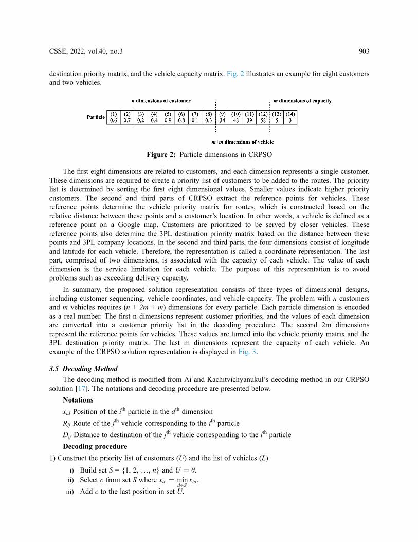
destination priority matrix, and the vehicle capacity matrix. Fig. 2 illustrates an example for eight customersand two vehicles.

The first eight dimensions are related to customers, and each dimension represents a single customer.These dimensions are required to create a priority list of customers to be added to the routes. The prioritylist is determined by sorting the first eight dimensional values. Smaller values indicate higher prioritycustomers. The second and third parts of CRPSO extract the reference points for vehicles. Thesereference points determine the vehicle priority matrix for routes, which is constructed based on therelative distance between these points and a customer’s location. In other words, a vehicle is defined as areference point on a Google map. Customers are prioritized to be served by closer vehicles. Thesereference points also determine the 3PL destination priority matrix based on the distance between thesepoints and 3PL company locations. In the second and third parts, the four dimensions consist of longitudeand latitude for each vehicle. Therefore, the representation is called a coordinate representation. The lastpart, comprised of two dimensions, is associated with the capacity of each vehicle. The value of eachdimension is the service limitation for each vehicle. The purpose of this representation is to avoidproblems such as exceeding delivery capacity.

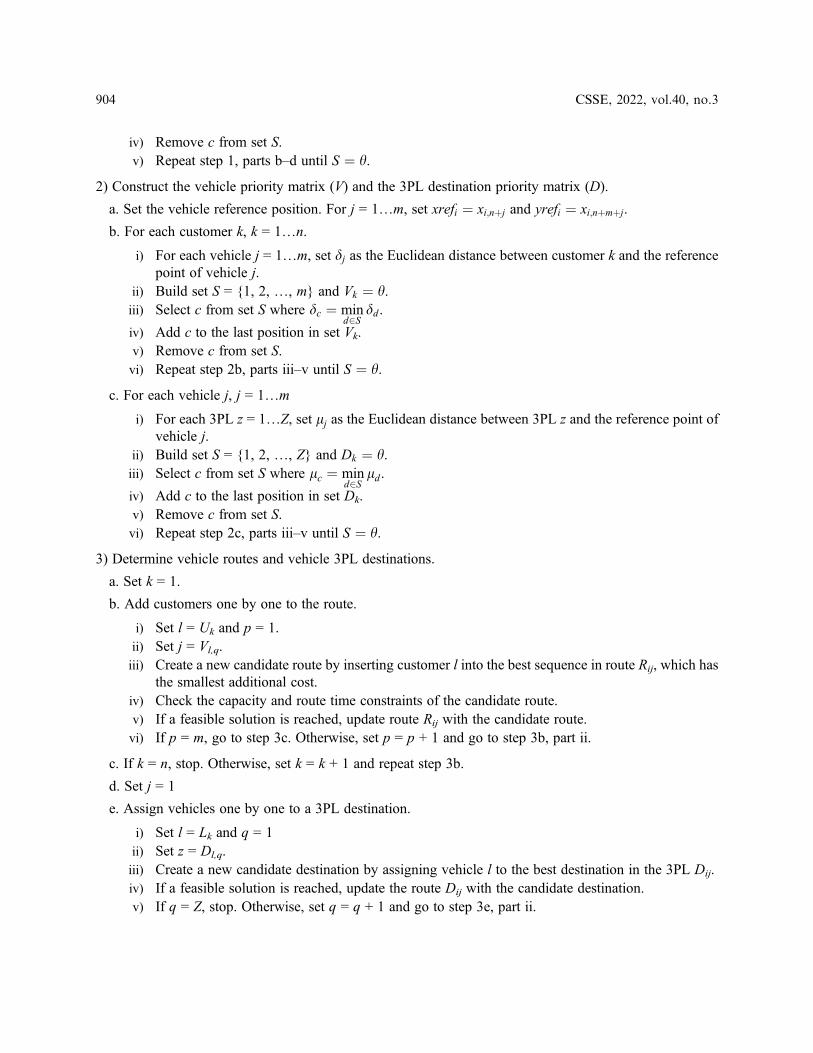
In summary, the proposed solution representation consists of three types of dimensional designs,including customer sequencing, vehicle coordinates, and vehicle capacity. The problem with n customersand m vehicles requires (n + 2m + m) dimensions for every particle. Each particle dimension is encodedas a real number. The first n dimensions represent customer priorities, and the values of each dimensionare converted into a customer priority list in the decoding procedure. The second 2m dimensionsrepresent the reference points for vehicles. These values are turned into the vehicle priority matrix and the3PL destination priority matrix. The last m dimensions represent the capacity of each vehicle. Anexample of the CRPSO solution representation is displayed in Fig. 3.

3.5 Decoding Method

The decoding method is modified from Ai and Kachitvichyanukul’s decoding method in our CRPSOsolution [17]. The notations and decoding procedure are presented below.

Notations

xid Position of the ith particle in the dth dimension

Rij Route of the jth vehicle corresponding to the ith particle

Dij Distance to destination of the jth vehicle corresponding to the ith particle

Decoding procedure

1) Construct the priority list of customers (U) and the list of vehicles (L).

i) Build set S = {1, 2, …, n} and U ¼ h.ii) Select c from set S where xic ¼ min

d2Sxid .

iii) Add c to the last position in set U.

Figure 2: Particle dimensions in CRPSO

CSSE, 2022, vol.40, no.3 903

iv) Remove c from set S.v) Repeat step 1, parts b–d until S ¼ h.

2) Construct the vehicle priority matrix (V) and the 3PL destination priority matrix (D).

a. Set the vehicle reference position. For j = 1…m, set xrefi ¼ xi;nþj and yrefi ¼ xi;nþmþj.

b. For each customer k, k = 1…n.

i) For each vehicle j = 1…m, set dj as the Euclidean distance between customer k and the referencepoint of vehicle j.

ii) Build set S = {1, 2, …, m} and Vk ¼ h.iii) Select c from set S where dc ¼ min

d2Sdd.

iv) Add c to the last position in set Vk.v) Remove c from set S.vi) Repeat step 2b, parts iii–v until S ¼ h.

c. For each vehicle j, j = 1…m

i) For each 3PL z = 1…Z, set lj as the Euclidean distance between 3PL z and the reference point ofvehicle j.

ii) Build set S = {1, 2, …, Z} and Dk ¼ h.iii) Select c from set S where lc ¼ min

d2Sld.

iv) Add c to the last position in set Dk.v) Remove c from set S.vi) Repeat step 2c, parts iii–v until S ¼ h.

3) Determine vehicle routes and vehicle 3PL destinations.

a. Set k = 1.

b. Add customers one by one to the route.

i) Set l = Uk and p = 1.ii) Set j = Vl,q.iii) Create a new candidate route by inserting customer l into the best sequence in route Rij, which has

the smallest additional cost.iv) Check the capacity and route time constraints of the candidate route.v) If a feasible solution is reached, update route Rij with the candidate route.vi) If p = m, go to step 3c. Otherwise, set p = p + 1 and go to step 3b, part ii.

c. If k = n, stop. Otherwise, set k = k + 1 and repeat step 3b.

d. Set j = 1

e. Assign vehicles one by one to a 3PL destination.

i) Set l = Lk and q = 1ii) Set z = Dl,q.iii) Create a new candidate destination by assigning vehicle l to the best destination in the 3PL Dij.iv) If a feasible solution is reached, update the route Dij with the candidate destination.v) If q = Z, stop. Otherwise, set q = q + 1 and go to step 3e, part ii.

904 CSSE, 2022, vol.40, no.3

4 Computational Results

This section compares the performance of the developed CRPSO algorithm to PSO using problems ofthe same scale, and evaluates the quality of the CRPSO solution by analyzing the computational results. Thissection consists of three parts: benchmark instances, parameter settings and PSO dimensions, and acomparison table. We tested our research experiments using Solomon’s 56 VRPTW benchmark instances[24] on a computer equipped with an Intel(R) Core(TM) i5-3210M 2.50GHz CPU and 4 GB RAMrunning the Microsoft Windows 7 operating system.

4.1 Benchmark Instances

We tested the proposed heuristic on three different data sets [24]. Solomon’s 56 VRPTW benchmarkproblems consist of six sets (C1, C2, R1, R2, RC1, RC2), each of which contains between 8 and12 problems; each data set has 100 nodes. C, R, and RC represent three different types of customer sets.C represents Clustered customers, R indicates randomly (uniformly) distributed customers, and RCrepresents Semi-clustered customers; that is, a combination of clustered and randomly (uniformly)distributed customers.

Figure 3: CRPSO solution representation

CSSE, 2022, vol.40, no.3 905

Moreover, C, R and RC problems can be further classified into two types: type 1 (C1, R1, RC1)problems have short time windows and small vehicle capacities, and type 2 (C2, R2, RC2) problemshave long time windows and large vehicle capacities. However, the proposed problem in this paper isOVRPTW considering 3PL, so the problem set differs from Solomon’s data [24]. Therefore, we dividedthe original 100 nodes in the experimental problem set into two groups; we assigned the first 90 nodes ineach problem to customers, and the remaining 10 nodes to 3PL companies. After a vehicle makes its finaldelivery, it must return to the nearest 3PL location with available space. Vehicle destinations are limitedto the 10 3PL nodes, but the capacity of each 3PL location is limited to three (i.e., only three vehiclescan return to each 3PL location). Hence, each vehicle must be assigned to a 3PL location according tothe 3PL destination priority matrix. If the nearest 3PL is full, the vehicle will return to the nearestlocation with available space.

4.2 Parameter Settings and PSO Dimensions

The parameter settings in PSO and CRPSO include population size as 100, iteration as 200, Cp as 2 andCg as 2. A PSO problem with n customers and m vehicles consists of (n + m) dimensional particles. Eachdimension in each particle is encoded as a real number, and the solution representation is divided intotwo parts. The first part is used to create a customer priority list by sorting the dimensional values.Smaller values indicate higher priority customers. The second part is same as the capacity dimensionin CRPSO.

4.3 Comparison Table

The proposed CRPSO algorithm and PSO was implemented using the Visual Studio C# programminglanguage. Some criteria can be used to evaluate the effectiveness of the developed CRPSO algorithm. Onecommon criterion is the solution gap between the optimal solution of PSO and the best solution found by theCRPSO algorithm. The experiments verify the solution to determine the improvement rate for travel distance.The solution gap is defined as below [25].

Solution Gapð%Þ ¼ S � B

B� 100% (30)

where B is the optimal solution obtained from the PSO result, and S is the optimal solution of theCRPSO algorithm.

All 56 data sets from Solomon’s problems [24] are tested and the results are shown in Tab. 1. In the table,TD is travel distance, NV is the number of vehicles used, and CPU is the computational time in seconds. Theobjective in this research is to minimize the total travel distance, that is, TD is viewed as an indicator ofsolution quality that enables the PSO and CRPSO solutions to be compared. Overall, the proposedCRPSO algorithm is effective at finding the shortest path to service all customers. Compared to the PSOresult, the average travel distances for all three problem types are shorter, as indicated by the solutiongap. Beyond the solution gap, NV is another important index to discuss.

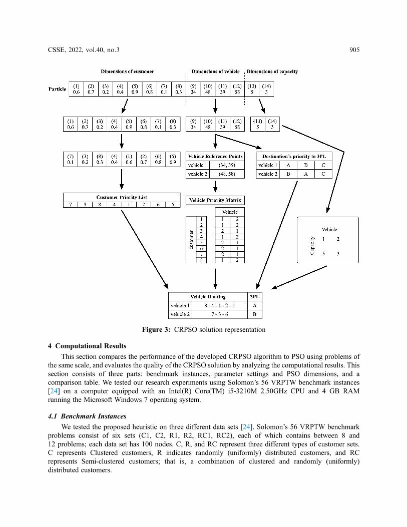
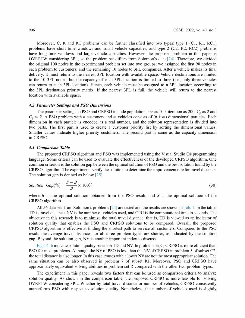
Figs. 4–6 indicate solution quality based on TD and NV. In problem set C, CRPSO is more efficient thanPSO for most problems. Although the NVof PSO is less than the NVof CRPSO in problem 5 of subset C2,the total distance is also longer. In this case, routes with a lower NVare not the most appropriate solution. Thesame situation can be also observed in problem 7 of subset R1. Moreover, PSO and CRPSO haveapproximately equivalent solving abilities in problem set R compared with the other two problem types.

The experiment in this paper reveals two factors that can be used as comparison criteria to analyzesolution quality. As shown in the comparison table, the proposed CRPSO is more feasible for solvingOVRPTW considering 3PL. Whether by total travel distance or number of vehicles, CRPSO consistentlyoutperforms PSO with respect to solution quality. Nonetheless, the number of vehicles used is slightly

906 CSSE, 2022, vol.40, no.3

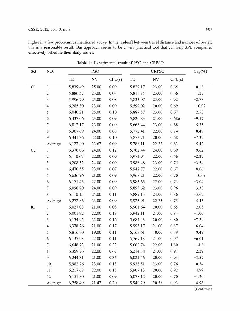
higher in a few problems, as mentioned above. In the tradeoff between travel distance and number of routes,this is a reasonable result. Our approach seems to be a very practical tool that can help 3PL companieseffectively schedule their daily routes.

Table 1: Experimental result of PSO and CRPSO

Set NO. PSO CRPSO Gap(%)

TD NV CPU(s) TD NV CPU(s)

C1 1 5,839.49 25.00 0.09 5,829.17 23.00 0.65 −0.18

2 5,886.57 23.00 0.08 5,811.75 23.00 0.66 −1.27

3 5,996.79 25.00 0.08 5,833.07 25.00 0.92 −2.73

4 6,285.30 23.00 0.09 5,599.02 20.00 0.69 −10.92

5 6,040.21 25.00 0.10 5,887.57 23.00 0.67 −2.53

6 6,437.06 23.00 0.09 5,820.83 21.00 0,686 −9.57

7 6,012.17 23.00 0.09 5,666.44 23.00 0.68 −5.75

8 6,307.69 24.00 0.08 5,772.41 22.00 0.74 −8.49

9 6,341.36 22.00 0.10 5,872.71 20.00 0.68 −7.39

Average 6,127.40 23.67 0.09 5,788.11 22.22 0.63 −5.42

C2 1 6,376.06 24.00 0.12 5,762.44 24.00 0.69 −9.62

2 6,110.67 22.00 0.09 5,971.94 22.00 0.66 −2.27

3 6,208.32 24.00 0.09 5,988.48 23.00 0.75 −3.54

4 6,470.55 23.00 0.07 5,948.77 22.00 0.67 −8.06

5 6,636.96 21.00 0.09 5,967.21 22.00 0.70 −10.09

6 6,171.45 22.00 0.09 5,983.65 22.00 0.73 −3.04

7 6,098.70 24.00 0.09 5,895.62 23.00 0.96 −3.33

8 6,110.15 24.00 0.11 5,889.13 24.00 0.86 −3.62

Average 6,272.86 23.00 0.09 5,925.91 22.75 0.75 −5.45

R1 1 6,027.03 21.00 0.08 5,901.64 20.00 0.65 −2.08

2 6,001.92 22.00 0.13 5,942.11 21.00 0.84 −1.00

3 6,134.95 22.00 0.16 5,687.43 20.00 0.80 −7.29

4 6,378.26 21.00 0.17 5,993.17 21.00 0.87 −6.04

5 6,816.80 19.00 0.11 6,169.61 18.00 0.89 −9.49

6 6,137.93 22.00 0.11 5,769.13 21.00 0.97 −6.01

7 6,648.73 21.00 0.22 5,660.74 22.00 1.80 −14.86

8 6,359.76 22.00 0.67 6,214.38 21.00 0.97 −2.29

9 6,244.31 21.00 0.36 6,021.46 20.00 0.93 −3.57

10 5,982.76 23.00 0.13 5,938.51 23.00 0.76 −0.74

11 6,217.68 22.00 0.15 5,907.13 20.00 0.92 −4.99

12 6,151.80 21.00 0.09 6,078.12 20.00 0.70 −1.20

Average 6,258.49 21.42 0.20 5,940.29 20.58 0.93 −4.96(Continued)

CSSE, 2022, vol.40, no.3 907

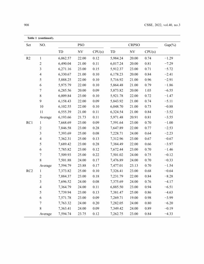
Table 1 (continued).

Set NO. PSO CRPSO Gap(%)

TD NV CPU(s) TD NV CPU(s)

R2 1 6,062.57 22.00 0.12 5,984.24 20.00 0.74 −1.29

2 6,490.04 21.00 0.11 6,017.24 20.00 0.81 −7.29

3 6,271.16 23.00 0.15 5,912.37 23.00 0.71 −5.72

4 6,330.67 21.00 0.10 6,178.23 20.00 0.84 −2.41

5 5,888.25 22.00 0.10 5,716.92 21.00 0.96 −2.91

6 5,975.79 22.00 0.10 5,864.48 21.00 0.79 −1.86

7 6,285.56 20.00 0.09 5,873.82 20.00 1.03 −6.55

8 6,009.84 23.00 0.10 5,921.78 22.00 0.72 −1.47

9 6,158.43 22.00 0.09 5,843.92 21.00 0.74 −5.11

10 6,102.55 22.00 0.10 6,048.70 21.00 0.73 −0.88

11 6,555.39 21.00 0.11 6,324.54 21.00 0.84 −3.52

Average 6,193.66 21.73 0.11 5,971.48 20.91 0.81 −3.55

RC1 1 7,668.69 23.00 0.09 7,591.64 23.00 0.70 −1.00

2 7,846.58 23.00 0.28 7,647.89 22.00 0.77 −2.53

3 7,393.69 25.00 0.08 7,228.71 24.00 0.64 −2.23

4 7,362.31 25.00 0.13 7,312.96 23.00 0.67 −0.67

5 7,689.42 23.00 0.28 7,384.49 22.00 0.66 −3.97

6 7,785.82 23.00 0.12 7,672.44 23.00 0.70 −1.46

7 7,509.93 25.00 0.22 7,501.02 24.00 0.75 −0.12

8 7,501.88 24.00 0.17 7,476.89 24.00 0.70 −0.33

Average 7,594.79 23.88 0.17 7,477.01 23.13 0.70 −1.54

RC2 1 7,373.82 25.00 0.10 7,326.41 23.00 0.68 −0.64

2 7,884.37 23.00 0.18 7,231.79 22.00 0.84 −8.28

3 7,696.52 24.00 0.08 7,375.69 24.00 0.76 −4.17

4 7,364.79 24.00 0.11 6,885.50 23.00 0.94 −6.51

5 7,739.94 23.00 0.13 7,381.47 25.00 0.86 −4.63

6 7,571.78 23.00 0.09 7,269.71 19.00 0.98 −3.99

7 7,763.32 24.00 0.20 7,282.05 24.00 0.80 −6.20

8 7,363.41 24.00 0.09 7,349.42 24.00 0.89 −0.19

Average 7,594.74 23.75 0.12 7,262.75 23.00 0.84 −4.33

908 CSSE, 2022, vol.40, no.3

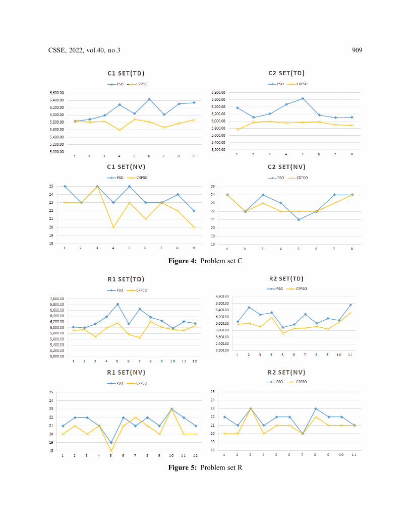
Figure 4: Problem set C

Figure 5: Problem set R

CSSE, 2022, vol.40, no.3 909

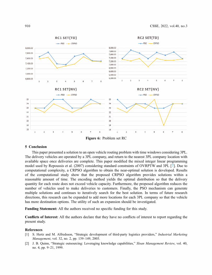
5 Conclusion

This paper presented a solution to an open vehicle routing problem with time windows considering 3PL.The delivery vehicles are operated by a 3PL company, and return to the nearest 3PL company location withavailable space once deliveries are complete. This paper modified the mixed integer linear programmingmodel used by Repoussis et al. (2007) considering standard constraints of OVRPTW and 3PL [7]. Due tocomputational complexity, a CRPSO algorithm to obtain the near-optimal solution is developed. Resultsof the computational study show that the proposed CRPSO algorithm provides solutions within areasonable amount of time. The encoding method yields the optimal distribution so that the deliveryquantity for each route does not exceed vehicle capacity. Furthermore, the proposed algorithm reduces thenumber of vehicles used to make deliveries to customers. Finally, the PSO mechanism can generatemultiple solutions and continues to iteratively search for the best solution. In terms of future researchdirections, this research can be expanded to add more locations for each 3PL company so that the vehiclehas more destination options. The utility of such an expansion should be investigated.

Funding Statement: All the authors received no specific funding for this study.

Conflicts of Interest: All the authors declare that they have no conflicts of interest to report regarding thepresent study.

References[1] S. Hertz and M. Alfredsson, “Strategic development of third-party logistics providers,” Industrial Marketing

Management, vol. 32, no. 2, pp. 139–149, 2003.

[2] J. B. Quinn, “Strategic outsourcing: Leveraging knowledge capabilities,” Sloan Management Review, vol. 40,no. 4, pp. 9–21, 1999.

Figure 6: Problem set RC

910 CSSE, 2022, vol.40, no.3

[3] M. Christopher, Logistics & supply chain management. New York: Pearson Publishing, 2016.

[4] G. B. Dantzig and J. H. Ramser, “The truck dispatching problem,”Management Science, vol. 6, no. 1, pp. 80–91, 1959.

[5] K. H. Leung, C. K. Lee and K. L. Choy, “An integrated online pick-to-sort order batching approach for managingfrequent arrivals of B2B e-commerce orders under both fixed and variable time-window batching,” AdvancedEngineering Informatics, vol. 45, pp. 101–125, 2020.

[6] J. E. Bell and P. R. McMullen, “Ant colony optimization techniques for the vehicle routing problem,” AdvancedEngineering Informatics, vol. 18, no. 1, pp. 41–48, 2004.

[7] P. P. Repoussis, C. D. Tarantilis and G. Ioannou, “The open vehicle routing problem with time windows,” Journalof the Operational Research Society, vol. 58, no. 3, pp. 355–367, 2007.

[8] P. P. Repoussis, D. C. Paraskevopoulos, G. Zobolas, C. D. Tarantilis and G. Ioannou, “A web-based decisionsupport system for waste lube oils collection and recycling,” European Journal of Operational Research, vol.195, no. 3, pp. 676–700, 2009.

[9] A. Baykasoglu and V. Kaplanoglu, “A multi-agent approach to load consolidation in transportation,” Advances inEngineering Software, vol. 42, no. 7, pp. 477–490, 2011.

[10] P. Amorim, H.-O. Günther and B. Almada-Lobo, “Multi-objective integrated production and distribution planningof perishable products,” International Journal of Production Economics, vol. 138, no. 1, pp. 89–101, 2012.

[11] I. Moon, J.-H. Lee and J. Seong, “Vehicle routing problem with time windows considering overtime andoutsourcing vehicles,” Expert Systems with Applications, vol. 39, no. 18, pp. 13202–13213, 2012.

[12] M. Dorigo, V. Maniezzo and A. Colorni, “Ant system: optimization by a colony of cooperating agents,” IEEETransactions on Systems, Man, and Cybernetics, Part B: Cybernetics, vol. 26, no. 1, pp. 29–41, 1996.

[13] L. Schrage, “Formulation and structure of more complex/realistic routing and scheduling problems,” Networks,vol. 11, no. 2, pp. 229–232, 1981.

[14] D. Sariklis and S. Powell, “A heuristic method for the open vehicle routing problem,” Journal of the OperationalResearch Society, vol. 51, no. 5, pp. 564–573, 2000.

[15] X. Li, P. Tian and S. C. Leung, “An ant colony optimization metaheuristic hybridized with tabu search for openvehicle routing problems,” Journal of the Operational Research Society, vol. 60, no. 7, pp. 1012–1025, 2009.

[16] K. Fleszar, I. H. Osman and K. S. Hindi, “Avariable neighbourhood search algorithm for the open vehicle routingproblem,” European Journal of Operational Research, vol. 195, no. 3, pp. 803–809, 2009.

[17] T. J. Ai and V. Kachitvichyanukul, “Particle swarm optimization and two solution representations for solving thecapacitated vehicle routing problem,” Computers & Industrial Engineering, vol. 56, no. 1, pp. 380–387, 2009a.

[18] T. J. Ai and V. Kachitvichyanukul, “A particle swarm optimization for the vehicle routing problem withsimultaneous pickup and delivery,” Computers & Operations Research, vol. 36, no. 5, pp. 1693–1702, 2009b.

[19] R. Eberhart and J. Kennedy, “A new optimizer using particle swarm theory. Paper presented at the MHS’95,” inProceedings of the Sixth International Symposium on Micro Machine and Human Science, Nagoya, Japan, 1995.

[20] J. Clarke, L. McLay and J. T. McLeskey Jr, “Comparison of genetic algorithm to particle swarm for constrainedsimulation-based optimization of a geothermal power plant,” Advanced Engineering Informatics, vol. 28, no. 1,pp. 81–90, 2014.

[21] A. Elbir, H. İlhan and N. Aydın, “The implementation of optimization methods for contrast enhancement,”Computer Systems Science and Engineering, vol. 34, no. 2, pp. 101–107, 2019.

[22] X. Wang, S. Liu and L. Zhang, “Highway cost prediction based on LSSVM optimized by initial parameters,”Computer Systems Science and Engineering, vol. 36, no. 1, pp. 259–269, 2021.

[23] S. Nguyen, T. J. Ai and V. Kachitvichyanukul, Object library for evolutionary techniques ETLib: User’s guide.Thailand: High Performance Computing Group, Asian Institute of Technology, 2010.

[24] M. M. Solomon, “Algorithms for the vehicle routing and scheduling problems with time window constraints,”Operations Research, vol. 35, no. 2, pp. 254–265, 1987.

[25] T.-L. Chen, J.-T. Lin and S.-C. Fang, “A shadow-price based heuristic for capacity planning of TFT-LCDmanufacturing,” Journal of Industrial and Management Optimization, vol. 6, no. 1, pp. 209–241, 2010.

CSSE, 2022, vol.40, no.3 911