€¦ · a cornputer system for predicting heat-affected zone (haz) hardness and weld €eaues...

NOTE TO USERS

Page(s) not included in the original manuscript are unavailable from the author or university. The

manuscript was microfilmed as received.

This reproduction is the best copy available.

UMI

Predicting the Features of Structural Steel Welds

with Internet Technology

Shunsuke Morinishi, B.Eng.

A thesis submitted to the Facdty of Graduate Studies and Research

in partial tULfilment of the requirements for the drgree of

Master of Engineering

Ottawa-Carkton hstitute for Mechanical and Arrospacr E n g i n e e ~ g

Depanment of Mechanical and Aerospace Engineering

Carle ton University

Ottawa, Ontario

Canada

National Library Bibliothèque nationale du Canada

Acquisitions and Acquisitions et Bibliographie Services services bibliographiques

395 Wellington Street 395, rue Wellington OttawaON K1A ON4 ûttawa ON KiA O N 4 Canada Canada

The author has granted a non- exclusive licence allowing the National Library of Canada to reproduce, loan, distribute or sel1 copies of this thesis h microform, paper or electronic formats.

The author retains ownership of the copyright in this thesis. Neither the thesis nor substantial extracts fiom it may be printed or otberwise reproduced without the author's permission.

L'auteur a accordé une licence non exclusive permettant a la Bibliothèque nationale du Canada de reproduire, prêter, distribuer ou vendre des copies de cette thése sous la forme de microfiche/nlm, de reproduction sur papier ou sur format électronique.

L'auteur conserve la propriété du droit d'auteur qui protège cette thèse. Ni la thèse ni des extraits substantiels de celle-ci ne doivent être imprimés ou autrement reproduits sans son autorisation.

A cornputer system for predicting heat-affected zone (HAZ) hardness and weld

€eaues (size and shape of the weld bead), originally coded by Chan [l-9, 101 but herein

re-coded for the world wide web, is descnbed in this thesis. In faa the web version

consists of two systems: a "passive" Java based system intended for remote processing,

and an "active" neural network semer system, coded with PHP (Personal Home Page

Tools) and mySQL (Sequential Query Language), a data base management language

intended for central processing.

The passive system is based on the regression algorithms of Yurioka [l-7, 81,

Teresalci [ l-5,6] and S w k i [14] for computing H M hardness and on the work of

Chandel [Z-6, 71 for computing weld feanires. In addition, a module based on fiilly

trained neural networks for computing both HAZ hardness and weld features originated

by Chan [l-9,10) has been re-coded for web implementation. Since the passive weld

design tools are to be downloaded for remote processing by users, they have been coded

with the Java language because it is relatively p1atfon-n independent and therefore

available to almost anyone familiar with the world wide web.

The active weld design tools consist of BPN (backpropagation network) modules

designed for training on the server. Users are expected to submit training data in HTML

format (via a web browser - Netscape or Microsofi Explorer) to the server which accepts

and translates it for BPN processing. Among other things this permits "custom" training

which is an important consideration because the welding process is not al1 that well

Predicting Weld Features W~th Inteniet Teckmolam

controlled and operator traditions often &éct the outcorne. M e r training the BPN modei

is then stored dong with the training data in a server database. Users can recall the model

for computing HAZ hardness or weld features as required.

One of the advantages of the active system is that user data and models are to be

captured by the server. By so doing, it is anticipated that a large data base of weld sizes

and shapes, and HAZ hardnesses, documented agauist operating parameters, can be

assembled for the benefit of the entire welding engineering community. Central server

processing to provide a data base of users, and weld data, is original insofar as this

researcher knows. The research and methodology used to generate this system is

descnbed in this thesis.

1 would like to express my deepest appreciation to my thesis supervisors, Professor

Malcolm Bibby and Dr. Billy Chan for their continued interest, encourasement and -idance

provided during this thesis program and throughout my study at Carleton university.

For the help 1 received in dealing with the web server system (PHP. MySQL, Apache), 1

extend my sincerest thanks to Roy Gibbons fiom the Faculty of Graduate Studies, and Kenji

I d fiom the Department of Computer Science.

I thank Professor Bibby and the Department of Mechanical and Aerospace Engineering,

Carleton University for their financial support. 1 would also like to thank all my fnends and the

staff of the Depariment of Mechanical and Aerospace Engineering at Carleton university for

their help and co-operation.

Finally, 1 would like to present this thesis to my beloved parents.

... I l l

Tdle of Contents

Page

Table of Contents

Lit of Figures

List of Tables

Nomenclature

Chapter One Int?oduction - 1.1 Weld Problem

1.2 Weld Models 1.3 Web Based Weld Pmperty Estimating Tool

Chapter Two Background 2. t Fusion WeId 2.2 WeId Structure and Metallurgy 2.3 Computational Models b Re ession Analysis I gr 2.3.1 The 800 to 500 C Cooling Time

2.3.2 HAZ Hardness Regression Models 2.3.2.1 Suzuki Model 2.3.2.2 Teresaki Mode11 2.3.2.3 Teresaki Model II 2.3 -2.4 Yurioka Model 1 2.3.2.5 Yurioka Mode1 II

2.3.3 Predicting Weld Features 2.3.3.1 Chandel Weld Features mode1

2.4 Computational Models by BackpropagationNetwork (BPN) 2.4.1 Backpropagation Network (BPN)

2.4.1.1 Falrnan's Derivative 2.4.1.2 ûther issues of Backpropagation Network

2.4.2 BPN HA2 Hardness Model 2-4.3 BPN Weld Features Mode1

2.5 A Web B a d Internet "Weldsofi" System

Chapter Tbree n e Web Based Regression System 3.1 The Regression Cooling Time Module

3.1.1 Venfication of The Regression Cooling Time Module 3 -2 The Regression HAZ Hardness Module

3.2.1 Verification of the Regression HAZ Hardness Module 3.3 The Regression Weld Features Module

3.3.1 Verifkation of the Regression Weld Features Module 3.4 Cornputer Requirements for the Web Based Regression System

Chapter Four The Web Based B P . System 4. I Tne BPEi Cooiing Time Module

4.1.1 Verification ofthe BPN Cooling Time Module 4.2 The BPN H M Hardness Module

4.2.1 Verification of the BPN HA2 Hardness Module 4.3 The BPN Weld Features Module

4.3.1 Verification of the BPN Weld Features Module 4.4 Cornputer Requirernents for the Web Based BPN System

Cha pter Five Web BPN Server System for Modeling ~ h e Welding Process 5.1 Hardware and Installed Applications Software 5.2 S ystern Implementation

5.2.1 Raw Data Submission Module 5.2.2 Selecting Training Data 5.2.3 Training Module 5.2.4 Weight Data Submission Module 5 2.5 BPN Cdculation Module 5.2.6 Data View Module

5.3 BPN Training Module Verificat ion 5.3.1 The XOR Problem 5.3 -2 The Cwling Time Problem 5.3.3 The tIAZ Hardness Problem

Chapter Six General Dismwbn

Cha pter S even Conclusions and Cunfrrfrrbutionr

Chapter Eight Futare Work

References

Appendix 1 Cooling Time Data

Appendix II AMC A Hardness Data

Appeodix III Gas Metal Arc Weld Size Data

Appendix IV SAW Experimentd Cooling Time

Appendix V Yurioka et al Experimental HAZ Hardness Data

Figure

L&s of Figure

Fusion welding with a positive polaity. 8

Three weId regions at a t-joint 10

Detaïled cross sectional area of a fusion weld and ironcarbon (steel) diagram

1 1

Schematic thermal cycle typical of a fixed position adjacent to a fusion weld

Weld heat fi ow rnorphology assumed in the RosenthaVAdams analyses.

HAZ CHC diagram.

Schematic diagram to define the constant K in the Sunrki approach for

cdculating HAZ hardness.

Schematic diagrarn to identie the feahires in the Chandel weld

features model.

Basic ANN structure.

Single node function.

A backpropagation network.

Simplified network weight - error relationship.

Weld bead rnodel cross section with bay len-gh and angle definition.

Flow diagram for the regression cooling time module.

User interface for the regession cooling time module.

vii

3 -3 Input area for the regession cooling time 53

3 -4 Parametnc study input area for the regression cooling time module. 54

3.5 Parametric output (coolhg time against voltage). 54

3.6 Message window for the regression cooling time module. 54

3.7 Comparison of calculated cooling tirnes (Adams model) with measured values: (A) 0-200 seconds range, (B) O - 60 seconds range). 57

3 -8 Flow diagram for the regression HAZ hardness module. 58

3.8 User interface for calculating HAZ hardness given (a) welding parameters and the chernical composition of the workpiece, (b) a measured cooling time and the chernicd composition of the workpiece. 59

3.1 1 Results ana (a) from 3-9a and (b) fiom 3-9b. 61

3.1 2 Parametric snidy input area for the regression HAZ hardness modules. 6 1

3.13 Plotting area for the regression HAZ hardness modules (a CHC is shown). 61

3.14 Comparison of meaaired (AMCA data) with calculated HA2 hardnesses: (a) Yurioka X, @) Yurioka II, (c) Terasaki I, (d) Terasaki II, (e) Suniki. 64

3.15 Flow diagram for the regression weid features module. 65

3.16 User interface for the regression weld features module. 66

3.17 Input area for the regreuion weld features module.

3.18 Output area for the regression weld features module.

3.19 Pictorial presentation of the regression weld features module. 67

3.20 Comparison of calnilated (Chandel rnodel) with meanired weld feanires

viii

(Northem college investigation - C2S gas cover): (a) bead height, @) bead width, (c) penetration, (d) deposited area, (e) fusion a r a 69

Comparison of calculated (Chandel model) with measured weld features (Northem college investigation - M 2 gas cover): (a) bead height, (b) bead width, (c) penetration, (d) deposited area, (e) fusion area.

Flow diagram for the BPN cooling time module.

User interface of the BPN cooling time module.

Input area for the BPN cooling time module.

Parametric study input area for the BPN.

Plot area for the BPN mling time module.

Cornpaison of measured cooling time with calailated values (a) O - 2005 1-5 BPN stnichire, (13)O - 200s, 2 4 3 BPN structure, (c) O - 60s, 1-5 BPN senidure, (d) O - 60s, 2 4 3 BPN structure.

Flow diagram for the BPN HAZ nardness module.

User interface for the BPN HAZ hardness module.

Input area for the BPN HAZ hardness module.

Parametric study input area for the BPN KAZ hardness.

Plot area for the BPN HA2 hardness module.

Chernical input area for the BPN H M hardness module.

Comparison of BPN calculated HAZ hardness

with measured values : (a) 1-4 BPN stnicture (b) 2 4 3 NPN structure. 8 1

Flow diagram for the BPN weld features module. 82

User interface for the BPN weld features module.

Input area for the BPN weld features module.

Result area for the BPN weld features module. 84

Plot area for the BPN weld features module. 84

Comparison of BPN calculated weld feature with measured values (Northem College investigation - C25 gas cover) (a) bead height, (b) bead width, (c) penetration, (d) bay length, (e) deposit area, (f) fusion area. 86

Comparison of BPN calculated weld features with measured values (Northem College investigation - MZ gas cover) (a) bead height, @) bead widtb, (c) penetration, (ci) bay lengtb, (e) deposited area, (f) fusion area. 87

Host - client cornputer configuration. 91

Flow diagram for the raw data submission module. 95

Generd data form for the raw data submission module. 96

General data confirmation screen for the raw data submission module. 97

Detailed data form for the raw data submission module. 98

Detailed data screen for the raw data subrnission module. 99

Raw data submission completion screen.

Flow diagrarn for the selecting training data.

Desired data condition input screen for the selecting training data.

List of raw data sets for the seiecting training data.

Detailed screen for the selecting training data

Data seleetion completion screen for the selecting training data.

Flow diagram for the training module.

General training conditions form for the training module.

List of training data sets for the training module.

5.16 Training condition summary screen for the training module. 1 07

5.17 Training cornpletion screen for the training moduie. 108

5.18 Training incomplete screen for the training module. 108

5.19 Weight set summary screen for the training module. 1 09

5.20 Weight set subrnission camplete screen for the training module. 110

5.21 Flow diagram for the weight submission module. 110

5.22 General infcrmation submission form for the weight data submission module. 112

5.23 General information confirmation screen for the weight data set submission module. 113

5.24 Detailed information submission form for the weight submission module. 114

5.25 Detail information confirmation screen for the weight submission module. 115

5.26 Weight data submission complete screen for the weight data set submission module. 116

5.27 Flow diagram for the BPN calculation module.

5.28 List of weight data set for the BPN caiculation module.

5.29 Input data submission form for the BPN calculation module. 118

5.30 Calculation resuh for the BPN caiculation module. 119

5.3 1 Flow diagram for the data view module. 120

5.32 Desired data conditions for the data view module.

5.33 List of data for the data view module. 122

5.34 Detailed data format) for the data view module.

5.35 Detailed data (text format) for the data view module.

5.36 Graphical representation of XOR problem.

xii

List of Tables Table

2- 1

2-2

2-3

2-4

2-5

2-6

2-7

2-8

2-9

2- 1 O

3-1

4.1

4.2

4.3

5 , t

5 -2

5 3

5.4

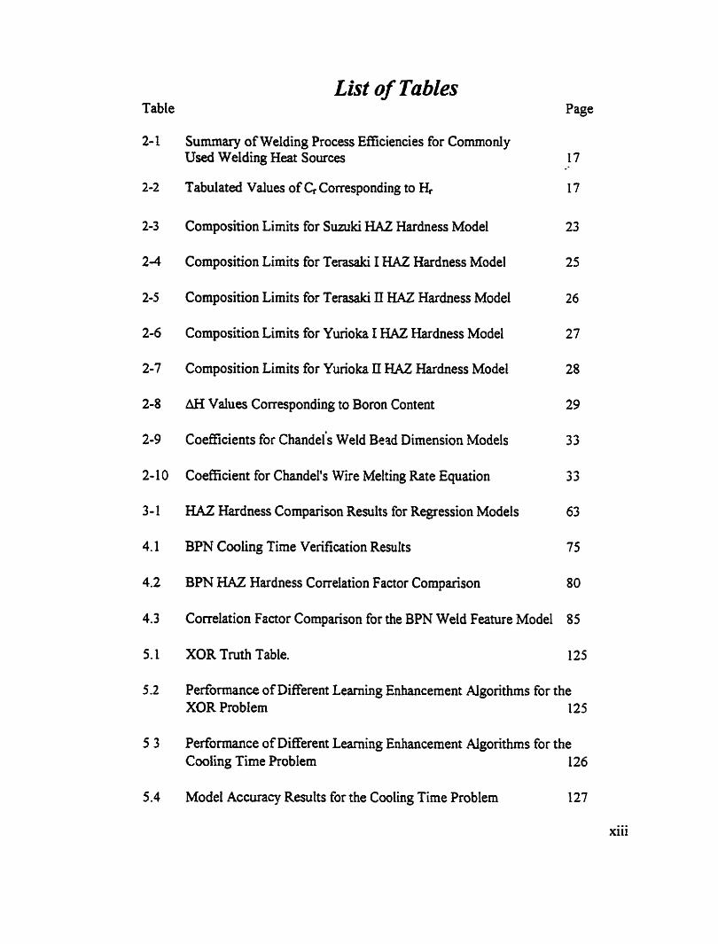
Summary of Welding Process Eficiencies for Comrnonly Used Welding Heat Sources

Tabulated Values of C, Corresponding to &

Composition Limits for S w k i HAZ Hardness Mode1

Composition Limits for Terasaki 1 KAZ Hardness Mode1

Composition Limits for Terasaki II KAZ Hardness Mode1

Composition Lirnits for Yurioka I HAZ Hardness Model

Composition Limits for Yurioka II HAZ Hardness Model

AH Values Corresponding to Boron Content

Coefficients for ~hande i s Weld B e d Dimension Models

Coefficient for Chandel's Wire Melting Rate Equation

HAZ Hardness Cornparison Results for Regression Models

BPN Cooling Time Verification Results

BPN HAZ Hardness Correlation Factor Cornparison

Page

17

17

23

25

26

27

28

29

33

33

63

75

80

Correlation Factor Cornparison for the BPN Weld Feature Model 85

XOR Truth Table. 125

Performance of Different Learning Enhancement Algonthms for the XOR ProbIem 125

Performance of Different Learning Enhancement Algorithms for the Cooling Time Problem 126

Mode1 Accuracy ResuIts for the Cooling Time Problem 127

Nomenclature

FZ - fusion zone HAZ - heat afEected zone IIW - the International Institute of Welding GMAW - gas metal arc welding SAW - submerged arc welding GTAW - gas tungsten arc welding bj - 80800 &O 50Q°C cooling tirne (sec j CTT - continuous cooling transformation CHC - characteristics hardness curve w10 - weight percent CE - IIW carbon equivalent (w/o) Pcm - Ito's carbon equivalent (w/o) CqI - C,Irr - Carbon equivalents (w/o) for Yurioka's first model CEi - CEm - Carbon equivalents (w/o) for Yurioka's second model B - boron content (w/o) C - carbon content (w/o) Cr - chromium content (w/o) Cu - copper content (w/o) Fe - iron content (w/o) Mn - rnanganese content (w/o) Mo - molybdenum content (w/o) Ni - nickel content (w/o) Nb - niobium content (w/o) Si - silicon content (w/o) V - vanadium content ( w/o) HVw - maximum HAZ hardness (VHN) b[3D] - thick plate cooling time fiom 800 to 500°C (sec) t~/~[2-D] - thin plate cooling time fiom 800 to 500°C (sec) k5[2.5-D] - intemediate plate cooling tirne from 800 to 500°C (sec) qpor - welding process efficiency (%) Q - heat input rate per unit Iength (J/s/mm) h, - plate thickness (mm) k - thema1 conductivity (J/(s.rnm.K)) Cp - volumetric specific heat ( ~ / ( m m ~ ~ ) ) 2 - plate initial temperature (OC) Cr - ratio of cooling time on thick plate to that on finite plate 1, - arc current (arnperes) V, - arc voltage (volts) S, - wire travef speed (mm/s) H, - relative plate thickness I - welding current (Amp) - weld feature model

V - arc voltage (volt) - weld feature model v - travel speed (rnmls) - weld feature model D - electrode diameter (mm) - weld feature rnodel L - electrïc extension (mm) - weld feature model MR - melting rate (ka) BW - bead width (mm) BH - bead height (mm) Pene - penetration length (mm) Al - deposited area (mm2) A2 - plate fusion zone (mm2) A - total fusion area (mm2) AI - artificial Intelligence ANN - artificial neural network BPN - backpropagation network I - input layer of backpropagation network H - hidden layer of backpropagation network O - Output layer of backpropagation network m - nurnber of input aodes e - intermediate input node n - number of hidden nodes r - intermediate hidden node t - nurnber o f output nodes g - intemediate output node @-m - weight between input and hidden layer w"-O' - weight between hidden and output layer a,b - counter P, - n-th daia set p - total number of training data set X\ - input of node 1, for data set P, yP", - target output at node Ot for data set P, F - transfer fwiction s*, - summation of node SO, - summation of node 4 E'- error of the network G - a general function notation q - leming rate AW - change in weight 6 - delta term RMS e m r - mot mean squared error a - momentun coefficient SD - standard deviation PHP - personal home page SQL - Smctured Query Language KIUL - Hypertext Markup Language

Chapter One

Zntruduciion Fusion welding is an important and often underestimated industrial process. In fact

80% of al1 steel tonnage is welded in one fom or another. Moreover, it is well understwd

that a joint (fasteneci by whatever means) is the critical area of a aeel stmcture or device. In

fact, dmost dl structural and device f~lures occur because ofjoint problems. The loss of

money and/or life when a pipeline or an airliner fails c m be devastating. The need for

research to improve the integrity of joints designed for structures and devices is therefore

evident .

In generai, welded joints are considered better than the alternatives (bolting, brazing,

etc.) because it is usually possible to match the strength of a weld to that of the base metal if

consumables are properly fonnulated and good welding technique is used. To a great

extent a properly designed weld provides continuity across the joint which combines the

workparts into one fiiily integrated syaem. The ideal joint is one where all mechanical

properties are perfectly matched to those of the workpiece so that the weld is in fact,

indistinguishable Eom the base metal.

1.1 Weid Probiems

Real welded joints are usually far fkom ideal. In praaicai terms joint strength

ovemtches base metal strength which c m cause non-uniform sain distributions when

extemal service loads are applied. Moreover, triaxial residual stresses fiom the welding

process are inevitably present even before the weld is put into service. But beyond

M c t i n a Weld Fahues With ùitmet Tochnolw

simple mechanical strength, it is not possible to match other important properties such as

toughness; fatigue strength and corrosion resistance, which renden welded joints wlnerable to

failure by several mechanisms, other than overload [l-11. The heat-afFected zone (HA Z), i.e.,

the base metal region adjacent to the weld that is inevitabiy adversely affected by the heat fiom

the welding pro-, is generally recognized as the most dificult area to cuntrol. Often the

toughness, fiitigue and stress corrosion properties of this region are iderior to those of the

unaffected base metd. Moreover, welding engineers are, more or iess, hoaage to the properties

that appear in this region because the chemistry of the base material cannot be changed in

general, although heat input adjustments, preheat andfor postheat provide some masure of

control. Nonetheless, HAZ properties often Iimit the service pe~ormance of welded joints.

Notwithstanding what was said in the last paragraph, it is the formation of so called cold

cracks (sometimes terrned underbead or hydrogen induced cracks) in the HAZ that is the most

serious limitation of the welding process. When the material next to the weld is heated, it is

autenitized. When austenite cools it decomposes and if it cools relatively rapidly, as it does in

many welding situations, the decomposition produa is a hard and bnttie phase called martemite.

At the sarne time hydrogen and vnter Kpor f?om the electrode coating and fluxes, and water

vapor fiom the atmosphere breaks dom chemically in the arc and nascent hydrogen is injected

into the weld pool. From the weld pool some of the hydrogen diffuses into the HAZ. The

combination of hard, brinie martensite, hydrogen h m the arc and residud tensile stresses that

form in the HAZ are conditions that favor the formation of cold aacks. They form spontaneously

in the temperature range flom about 250 OC to room temperature as the weld cools or in some

Chapter 1 htroduction 2

Predicting Wdd Feaîures With Internet Technologv

cases their formation may be delayed for anywhere up to five days after completion of

the weld. This is a well known characteristic of hydrogen cracking under other

circumstances (e-g. corrosion situations) and has ied to the term "delayed cracking".

It is evident fiom the description above that cold cracks can fom in the HAZ

men before a weld is put into service. They are very dangerous, because when such a

weld is loaded, high stress concentrations build up amund such crack tips, which can

cause them to propagate rapidly in a brittie manner to failure. In kct, pre-existing HA2

cold crack defects is a significant cause of weld failures [1-21.

Cold crack formation can be avoided if the welding conditions can be arranged to

lirnit the HAZ hardness level. In practice a h i t of about 320 VPN is imposed in most

routine welding situations [1-31. For highly loaded applications such as pipelines, a lirnit

of ZSOVPN is ofien specified. As it tum O* in service stress corrosion cracking is also

very sensitive to HAZ hardness and this also gives rise to the necessity of limiting the

hardness in this region.

1.2 Weld Models

In view of the importance of HAZ hardness in engineering practice, several

researchers have proposed regression based models for caiculating the level that would be

expected, given the welding parameters (aiment, voltage, welding speed, etc.) and

workpiece chemicai composition Included in these are the models of Suzuki [Ml,

Teresaki 11-5,6], and Yurioka [l-7,8]. These are the mon recent and seemingly the best

available, and are therefore the models that were included in the recent software system

generated by Chan for this purpose. A review of al1 hardness models may be found in Chan's

worQ199].

In addition to the regression based models, Chan [ 1 - 10, 1 1 ] proposed a neural network

system for determining HAZ hardnesses. This system has the advantage that it can be custom

"tminedn to accommodate welding traditions and skilis at one or another job shop or

manufactwing facility. Universal systems such as regression models are at best oniy approximate

because the welding process, even under well controlled automated manufaauring conditions, is

somewhat variable. Characterizhg such a system to ensure an unequivocal and accurate

operating description is difficult and yet regression and physical modeling requires this to be the

case. This is not to say that regression models are not usefùl; quite the contrary - practitioners

- find them very useful, even though it is well understuod that they may not be entirely accurate in

one situation or another. However, with neural technology, the traditions of a job shop or a

manufactunng operation can be capturai implicitly by "training" with data relevant to the

situation at hand. In this way the neural network system is expected to be flexible and sensitive

to local welding tradition.

Chan recently generated a software system including both regression and neural network

algorithm for predicting H M hardnesses [ l-9,l O], and for anticipating the size and shape of the

weld fusion zone. Like HAZ hardness, the size and shape of a weld are important to the welding

engineering community. However, in this case it is largely a productivity issue although weld

properties are also integral with weld features. Welding is costly in fact it is one of the principal

costs of metal mamfacniring and fabrication In general deep penetration, narrow welds are

Predicting Weld Ftatures With Internet Tezhnoiogy

considered to provide the highest productivity, but such welds are often difficult to arrange and

their integrity can be problematic. If the penetration is too deep, burn through dificulties c m

arise, especially for thin plate situations. On the other hand insufficient penetration of the root

region may occur when the heat input is smail. Moreover, most joints are "prepared" before

welding and there are a whole range of weld geumetry issues that must be taken into account to

optimize productivity on the one hand and weld properties (e.g. avoiding cold cracking, etc.) on

the other.

The regressionheural network system generated by Chan has been well received. In

particular, the n e u d network approach is thought to be the way to analyze process situations

such as welding where physical modeling is very diffiailt and where there is uncertainty in the

regression approach. However, this researcher hastens to add that physical modeling is very

important. Even though the neural network approach is usefbl, it does not yield any

understanding of the underlying physics and mechanisrns involved. In the end physical modeling

is the only way the welding process will be fblly understood and controlled.

1.3 Web Based Weld Propertv Estimatine Tool

A web based version of the Chan system is descnbed in this thesis. The objective of

generating a web based version of the system is to make it available to the world at large and, in

particular, to those in the engineering community who would have an interest in it. m i l e

publishing the details of the system in contemporary journals has been done, it is a large nep

f?om there to working code. If the entire system were to be instailed and housed on a web

Chapter 1 Introduction

Predictinp WeId Features WitR Internet TechnoIow

server, anyone who wants to access and use it can do so without having to regenerate the

code.

There are essentialiy three modules in the web based system. The fim module is

a re-coded Java based version of the regression module first established by Chan. By re-

coding with the Java Intemet lanpage; it is made available to dmost al1 Internet uen

since such a system is relatively pladorm independent. Usen c m download this module

to their remote penonal cornputers and use it in a straightforward manner, i.e., welding

parameten are submitted and caiculated HAZ hardnesses or weld features are returned.

In Mme sense this can be viewed as a universal system for calculating HAZ hardness and

weld features.

In addition, a second Java module, based on a pre-trained neural network is

included in the web system. In practice using this module is similar to the way the

regression module is used and it cm be considered universal in the same sense. [t serves

as a second output for determining HAZ hardness or weld features which is usehl

considering the uncertainty in such calcuiations.

To permit Zustom trainingw as discussed previously, an untrained neural network

module has been made available to usen as part of the web system. However, the neural

network module is to be used only on the server via remote control fiom any web

connected worksution, Le., down Ioading wilI be prohibited. Usen of the web based

system will be asked to leave their names and affiliations, their training data, and their

hained models. In this way it is anticipated that a worldwide database of researchen,

Pdictinn Weld Features With Intemet Technolosy

practitioners, welding data, and several tmined models wiil be assembied for the benefit

of the entire welding community.

While the system is not yet in practice (the issue of semer maintenance has still to

be decided), the equivaient of a rnanufacturing "pilot plant" has been generated for this

thesis. The welding technology bais for the system is reviewsd in the following section.

Chapter 1 Introduction - .

Chapter Two

Background

To understand fblly the proposed web based system for predicting HAZ hardness and

weld features, it is necessary to review the welding process itself (section 2. l), the metallurgical

changes that give rise to the mechanica! properties of a defa free weld, the occurrence of

underbead cracks that so limit weid performance in service (section 2.2), and finally the HAZ

hardness and weld shape algonthms that are to be incorporated into the system (section 2.3, 2.4,

and 2.5).

2.1 Fusion Weld

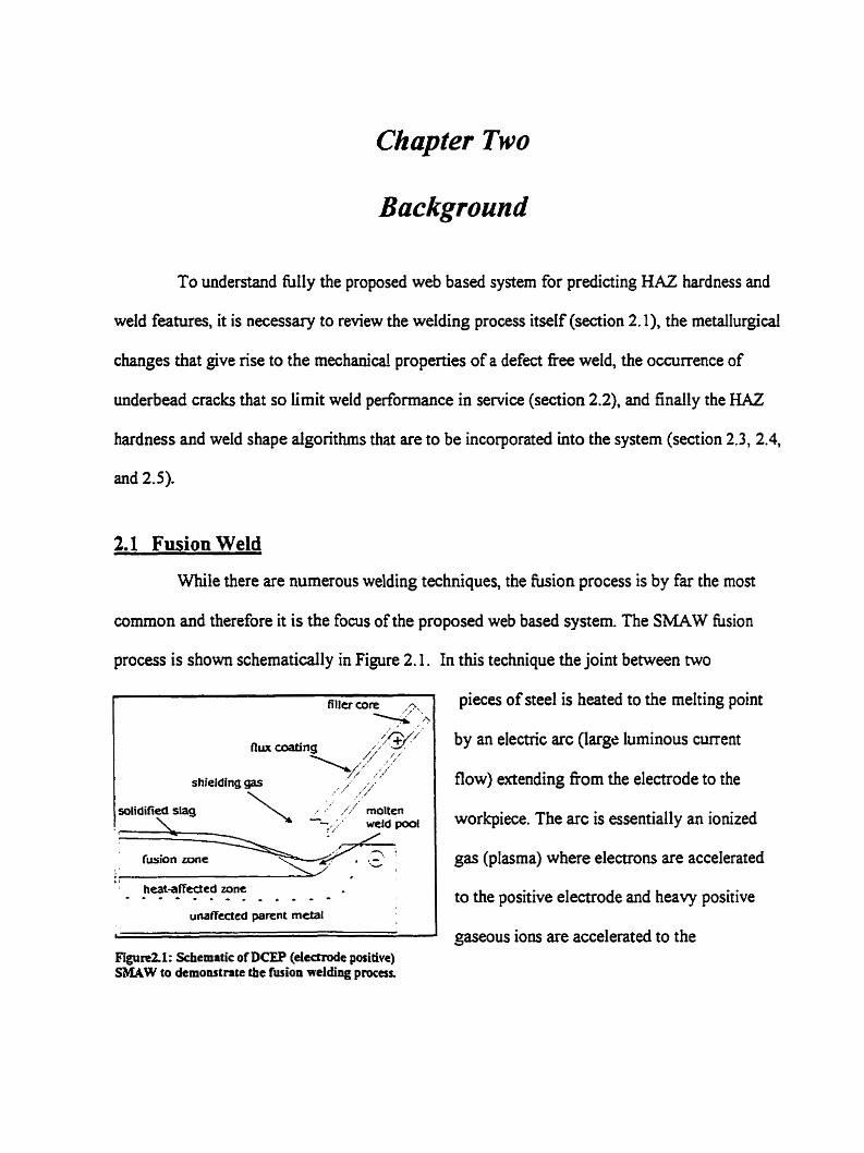
Whik there are numerous welding techniques, the fusion process is by far the most

common and therefore it is the focus of the proposed web based system. The SMAW fusion

process is show schematically in Figure 2.1. In this technique the joint between two

heatafFeded zone

unaffecîcd parent metal

Fïigure21: Schematic of DCEP (dectrode positive) SMAW to demonstrate the fuion we1ding procesr

pieces of steel is heated to the melting point

by an electric arc (iarge luminous curent

flow) extending from the electrode to the

workpiece. The arc is essentially an ionized

gas (plasma) where electrons are accelerated

to the positive electrode and heavy positive

gaseous ions are accelerated to the

Predictinp Weld Features With intemet Technology

negatively charged workpiece. When electrons strike the electrode and ions strike the

workpiece they lose kinetic energy which appears as heat. The intense heat of the arc causes a

local molten pool to f o m under the arc which re-solidifies to fuse the joint which in twn,

foms one continuous workpiece. The electrode not only serves as an essential electncal

element for the arc, but it is also the source of filler material for the joint. Mon joints are

shaped to a V or K configuration for alignment purposes and to receive molten filler metal

fiom the electrode. As the welding proceeds, the electrode is consumed and eventually has to

be replaced.

As shown in Figure 2.1, a typical electrode is covered with a flux coating which, upon

melting, forms a shielding gas and a slag layer on the molten pool. Both the shielding gas and

the slag layer serve to protea the pool from atmospheric oxidation. If there were not some

form of protection for the molten pool, oxide inclusions would otherwise seriously degenerate

the mechaaical propertîes of the joint.

The arrangement shown in Figure 2.1 above is known as the shielded metal arc (SMA)

process or sometimes called rnanual welding. An automatic version of this is the gas metal arc

(GiviA) process where a continuous wire feed replaces discrete length electrodes so that

continuous welding is possible. In addition, an inert gas, such as COt or argon, replaces the flux

that protects the molten pool. A review of other automatic welding processes such as the

submerged arc, plasma arc, electron beam or laser processes may be found in reference [2-261.

While joints are prepared in most welding situations, the arrangement show in Figure

2.1, where the weld is deposited on the surfàce of a workpeice, may be interpreted

C haptcr 2 Background

Predictine Weld Features Wth Internet Technoloey

as bead-on-plate (BOP). BOP welds are used to simulate joint welding situations for

expenrnental purposes rather than for joining paris per se. The BOP procedure is

relatively simple and tecechnical erroa are rninimized with such an arrangement so that

ski11 related parameten such as the heat input efficiency can be used with some

confidence. Moreover, BOP we!ds have b c n used extensivety by researchers to

study the welding process in generd and there is considerable experience with this

configuration. For example, the heat flow morphology is relatively well understood for

the BOP situation which is an important consideration. Yet the information gathered

from such investigations can, in generd, be a&pted to other more common welding

configurations and situations. In fact, the databases that fonn the basis for the web based

KAZ hardness, and weld features system described in this thesis are derived pnmanly

fiom GMA BOP weld expenmentr.

2.2 Weld Structure and Metalturgv

1 Hear~ectedzone I Figurc2.2: Th= wefd regions at a t- joint (FL HAL and d i & & base met& shmn scticmaticaiIy for a T joint configuration. A h shoun is an undcrbead crack which c;t? form in some c ~ m t a n c e s ) .

The intense heat source used in the fusion

welding process induces crystal growth in the

base metal adjacent to the joint In fact, three

distinctive regions form in a welded joint: the

fusion zone (FZ), the heat affected zone ( H M )

and unaffected parent metal as show

schematicaily in Figure 2.2. The microsmicture

changes rather dramatically from one zone to

-

Chapter 2 Background

Predictine Weld Features With Intemet Technolo~

another and therefore the mechanical propedes wouid be expected so v q with position

accordingl y.

A detailed cross section of

a fusion welded joint (Figure 2.3)

is shown together with pan of the

iron-carbon phase diagram to be

used for explanation purposes. To

understand the mechanisrns that

give rise to the microstnictures

and zones that appear adjacent to a

fusion wetd, it is first necessary to Figure2.3: Detailed cross section area o f a fusion weid and iroaurbon (steel) phase diagram [2-21.

appreciate the thermal changes that ammpany the process. Each fixed position adjacent

to the weld centerline experiences a thermal cycle similar to that shown schematically in

Figure 2.4.

As the heat source approaches a particular fixed position, the temperature first

inmeases, reaches a maximum (peak temperature) and then decreases. It is intuitive that

peak temperature decreases with distance fiom the weld centerline. Where the peak

tempera- exceeds the melting temperature (approximately 1 500 OC), fi Iler and base

metai melt during heating and re-solidifies upon cooling to form the hision zone (FZ) - region (a) in Figure 2.3. The grain rnorphology in this region is a coarse gained

columnar m c t u r e containing a dendntic subsmicture that refl ects the solidification

mechanism. Adjacent to the FZ is the KAZ, which can be divided further into four


Predictino Wetd Features With Internet Technology

subsections; the grain growth zone (b), the reciystdlized zone (c), the partially

transformed zone (d) and a tempered zone (e). Rapid grain growth is experienced in the

range from the mefting temperature to about ! 100°C. This leads to a relatively coane

grained equiaxed zone - region (b). The range of peak temperatures for the recrystallized

zone (cl is Rom about 1 100 O C to the Aj

(autenite-femte phase boundary). The

microstructure in this region is relatively fine-

grained because the phase transformation causes

recrstalIization but there is limited time and

temperatme for grain growth to mur. Region

(d) where the peak temperatme is between A3

the J

Figure 2.4 Schematic thermal cycle typical of a furcd position adjacent to a fusion wdd (2-31. (Note the 800°C to 500°C coolmg time which is uscd to charactcrizc a weld t h d cycle.)

and Al (eutectoid temperature) is called the partially transformed zone. Since the peak

ternperature does not reach A3 in this region, there is only partial austenitization and

mixed grains (original base metal femte/pearIite and decomposeci austenite products) CO-

exist. Peak temperature below Ai (approximately 720°C for carbon steel) but above

about 580 O C gives rise to the so-called tempered zone - region (e), there is some

recrystallization if there has been prior cold work in this region; othenvise not much else

happens. 580°C is approximately the lower limit of significant thermal activity in steels

and therefore peak temperatures below this temperature leave the base metai virtuaily

unaffected.

While the above discussion explains the occurrence of the FZ, and the HAZ

(together with subzones), it is not possible to rationaiize the microstnictures that might

Ptedictinn Weld Features With internet Tecfmolopy

occur in these regions frorn the equilibriurn diagram in the sarne way. This is because the

austentite decomposition products that are to be expected, depend on the rate of cooling.

If the cooling rate is hi& a high hardness, brittle decomposition product called

rnartensite appean in the HAZ. On the other hand if the cooling rate is not as fast, less

brittle products such as bainite or femtdpearlite form. The most sensitive produa is

martensite and as discussed in the introduction section, this is the phase that gives nse to

underbead cold crack formation (Figure 2.2).

It has become customary to characterize the cooling behavior of a weld by its

800°C to 500°C cooiing time t8/5. Among other things, this is the transformation range

(austenite decomposition) and as such it is considered to be the most sensitive region of

the thermal cycle. While cooling times would reasonably be expected to vary across a

we14 it tums out that the weld centerline cooling time does not differ substantially from

the cooling time of the coane grained KAZ [2-41, which as noted eariier is the mon

sensitive region of a weld. It is therefore, customary to speak of one single weld cooling

time for a fusion weld. Cooling times range from about 1s for a very small weld to about

100s for a very large weld. KAZ martensite c m be expected in the low cooling time

(high cooling rate) range, whereas there is less tendency for the formation of martensite

when the cooling t h e is high (slow cooling rate).

However, the tendency to fom manensite in the HAZ depends not only on the

cooling time but also on the "hardenability" of steel which, in tum, is a fmction of the

grain size and chemicai composition- The larger the austenite grain size, the greater the

tendency for martensite formation. As it tums out, the effect of grain size on

C hapter 2 Background

Predjctinn WeId Featiires With Interna Technotogy

hardenability is substantial - so much so that there is, in general, Iittle concem for the HAZ other

than the coarse grained region next to the FZ. Moreover, the "richer" the chernical composition,

the higher the hardenability and the greater the tendency for martensite to f o m It is well known

that carbon has the greatest effect of d l alloy additions on hardenability and therefore it is

customary to express the hardenability of the HAZ of steel welds in terms of a so-called "carbon

q u i d e n t " (CE).

Finally, the hardness of the coane grained HAZ depends not only on the tendency for

martensite to form in that region but dso on the inherent hardness of the martensite itself. To a

fist approximation, the hardness of martensite depends oniy on the carbon content. Therefore,

low carbon mensites are relatively soft and less prone to cracking t h higher carbon

martemites. In this regard the carbon content of filler materiais (electrode compositions) is

nomally kept intentionally low (Cc 0.05w/o) compared with base compositions of

O.O5w/o<C<0.3w/o [2-51. Because of this, the maximum hardness of a weld is usually found in

the HAZ, with the exception of Iow carbon microally steels where the carbon content ofthe filler

can exceed that of the base metal. To compensate for the loss of strength in the FZ, as a result of

low carbon levels, the low alloy content (Mn, Si, Cr, Ni Mo primarily) usually exceeds that of

the base metal. This of course, leads to high hardenability and encourages the formation of

martensite. However, the martensite so fomed is usually of low hardness and less sensitive to

cracking than the relatively higher hardness manensite of the coarse grained W.

It is apparent from the foregoing discussion that HAZ hardness is a fùnction of cooling

time, low alloy content (Le., hardenability) and carbon ievel (reflected by the inherent martensite

Predicting Weld Features With Internet TechnoIo&

hardness) of the base metal. Therefore, these factors must be included in any models for

predicting maximum HAZ hardness. HAZ hardness formulations are discussed in the

following section.

2.3 Computational Models bv Regression Analvsis

To compute HAZ hardness fiom the regression expressions aMilable for this purpose,

it is frst of ail necessary to determine a cooling time f?om the welding parameters. An

experimentai value (measured by injecting a thennocouple into the weld pool) can be used

but more often than not it is not available. If it is not available then it is necessary to calculate

it fiom the welding parameters. The cooling time is then submitted dong with the chernical

composition of the base material to the hardness models ( S d , Yunoka (two models) and

Teresaki (two models)) to determine HAZ hardness. The background necessary to calculate

cooling times and subsequently HAZ hardness is given in 2.3.1 and 2.3,2 respectively. In

2.3.2, there are five subsections, one for each HA2 model implemented for web system. In

addition, weld feahires modeling is dwcribed in 2.3.3 and the regression model of Chandel et

al [2-6,7] for this purpose is doaimented in 2.3.3.1. The background necessary to understand

the neural network technique used in this thesis for calculating HAZ hardness and for

estimating weld features is given in 2.4.1, 2.4.2, and 2.4.3, and the proposed web based systern

is discussed in 2.5.

2.3.1 The 800 to 500 OC Cooling: Time Mode1

As discussed in the last section, it is usually neces- to caicuiate an 8 0 0 ~ ~ to 500 OC

coolhg time, b5, h m the input welduig parametm (voltage, cumnt, welding speed, preheat


Predictîng Weld Fatures With Internet Technologv

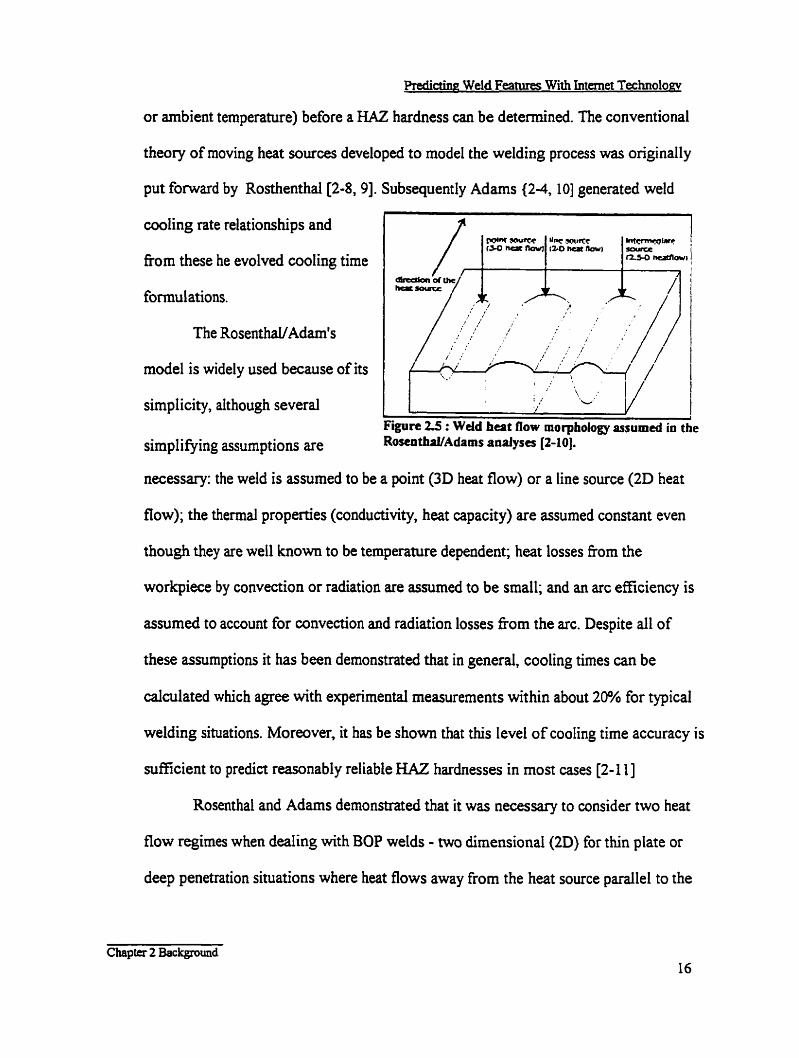
or arnbient temperature) before a HAZ hardness can be detennined. The conventional

theory of moving heat sources developed to mode1 the welding process was originally

put fonvard by Rosthenthal[2-8,9]. Subsequently Adams {2-4,101 generated weld

cooling rate relationships and

from these he evolved cooling time

formulations.

The RosenthaVAdamts

mode1 is widely used because of its

simplicity, although several I ' t' v I Figure L5 4: Wdd heat flow morphoIogy assumed in the - -

simplifiing assurnptions are RosuithrYAdarns anaiysa (2-la.

necessary: the weld is assumed to be a point (3D heat flow) or a Iine source (2D heat

flow); the thermal properties (conductivity, heat capacity) are assumed constant even

though they are well known to be temperature dependent; heat losses fkom the

workpiece by convection or radiation are assumed to be small; and an arc eEciency is

assumed to account for convection and radiation losses from the arc. Despite dl of

these assumptions it has been demonstrated that in general, cooling times can be

calculated which agree with experimental measurements within about 2Ph for typical

welding situations. Moreover, it has be show that this level of cooling time accuracy is

sufficient to predict rea~nably reliable HAZ hardnesses in mon cases [2-111

Rosenthal and Adams demonstrated that it was necessary to consider two heat

flow regimes when dealing with BOP welds - two dimensional (2D) for thin plate or

deep penetration situations where heat flows away from the heat source parallel to the

Chaptn 2 Background

Predicting Weld Features Wiîh Internet Technolow

plane ofthe workpiece (Figure 2.5) and three dimensional (3D) where the workpiece is

thick and heat flows not oniy parallel to the plane of the workpiece but also in the

through thickness direction. if the heat flow is intermediate, i.e., mked 2D/3D, it is

treated as a mixed morphology situation and is referred to as 2.SD heat flow. The Adams

ccoling time relationsfiips for 3D, 2 0 and 2.SD sinrations are as follows:

Table 2-1 Sumrnary of Welding Process Efficiencies for Commonly Used Welding Heat Sources

Process S W W SAW GMAW GTAW FCAW Efficiency % 80 95 70 40 70

Table 2-2 Tabulated Values of Cr Correspondhg to Hr

Equation 2- I

1 I ~ , Q t,,[2-D] = - 1 P - c 1 ( ) ' [( 500 - )'] Equation 2-2

2nkCp h, 800 - T,

Equation 2-3

where Q is the welding process energy input rate pet length in (Jlmm):

Equation 2-4

qros is the welding process efficiency (Table 2- L ), k is the thermal conductivity (0.025

J/(mm.s.K) is used), T, is the initial plate temperature, C, is the volumetric specific kat

(0.006 J ! ( ~ ' K ) is used), h, is the plate thickness in mm, Cr is a transition cooling time

Predictine Wcid Fcatirrcs With Intemet Technolo~y

parameter- the ratio of the thick plate cooling time to that of the finite plate (discussed

below) and L, Va, and S, are arc current in amperes, voltage in volts, and wire travel

speed in r n d s respectively.

The appropnate kat flow relationship to be used is determined by a relative

thickness parameter (Hr) defined as:

IfHr is greater than 1, the 3D relationship is used. If the Hr value is Iess than 0.3,

the 2D cooling mode1 is appropriate. In the Hr range between 0.3 and 1, the 2.5D mode1

is applied. Values of the parameter, Cr, are obtained fiom Table 2-2 corresponding to the

calculated value of Hr.

In the web based system described in this thesis, Equation 2-5 is computed to

identm th2 heat flow regime. Then a cooling time is calculated with one of the

relationships, equations 2-1 to 2-3, whichever is appropriate. The cooling time so calculated

is then submitted to one of the modeis document& in the next section to calculate a HAZ

hardness.

2.3.2 HA2 Hardness Regression ModeIs

The HAZ hardness regression models originated by Suniki [2-121, Teresaki [2-

13, 141 and Yurioka [2- 1 5,161 are incorporateci in the web based software described in

this thesis. While there are several other similar regression models in the literature, it is

widely held that these models are the best available. For example it is well known that

Chapter 2 Background 18

9

these models are based on high quality databases and thai they are well documented, i.e,

the cornpositional iimits are well defined in each case, among other things. In general

these models predict relatively accurate HAZ hardnesses if the compositional limiis are

respect& At the same time the cornpositional limits incorporate a relatively wide range

of low alloy and microalloy steels which are the matends of mon interen XI

praaoners.

There is a case to be made for including all available models in the wrb systrm

becaw they are regression based and therefore the accuacy and range of applicability is

always open to question It is the view of many researchers and practitioners that

computations from a wide range of models would provide a better bais for making

judgment. This was the philosophy uxd by Chan who reviewed al1 modcls and includcd

them in his original work [2- 17. However, it was decided that for this investigation,

including al1 models unnecessarily complicates the software. This is an important

consideration when impiementing the system on the web. ïherefm in the end it was

decided to irnplament oniy the Suzuki, Teresaki and Yurioka models. Othrr regession

expressions can be added in funire, if this is found to be a deficiency.

It is well understd in metaliurgical science that a phase diagram such as that

shown in Figure 2.3 is a fundamental and usefiii temperature/composi tion map of phases

under equilibrium conditions. Yct the thermal situation during welding is certainly not

equiiibnurn during cooling aithough it can reasonabiy be assumai when the joint is being

heated Transformation rates increase exponentially widi temperatm. Therefore during

the heating part of the thermal cycle, phase changes take place quickiy and it is wideiy


Predictài~ Weld Feattms With Intemet Tcchnology

held that near equilibrium can be assumed. This is why the phase diagram is used to

rationalize the extent of the HAZ as discussed in section 2.2 (Figure 2.3). However phase changes

are much more sluggish in the cooling part of the cycle and in partiailar hardened phases

includig the bainites and martensite c m form under relatively high cooling rate conditions.

In conventiond hait ndng, standard CCT diagrams (continuous cooling transformation

diagrams) are used to predict the phases that would be expected in one situation or another. CCT

diagrams generally reflect the material property known as hardenability, i.e., the greater the

tendency to form hardenable products, the greater the hardenability. It is well known that the

hardenability of a steel depends both on alloy content and austenite grain size. However, it is

difficult to apply standard CCT diagrams to the welding situation because the austenitization

temperature is high in the corne grained KAZ region and the ccoling time is short, quite unlike

anything enmuntered in normal heat treating. Therefore special CCT diagrams are used for the

welding situation where the mling tirne nom 800 OC to 500'~ is the abscissa rather than heat

treating time at temperature.

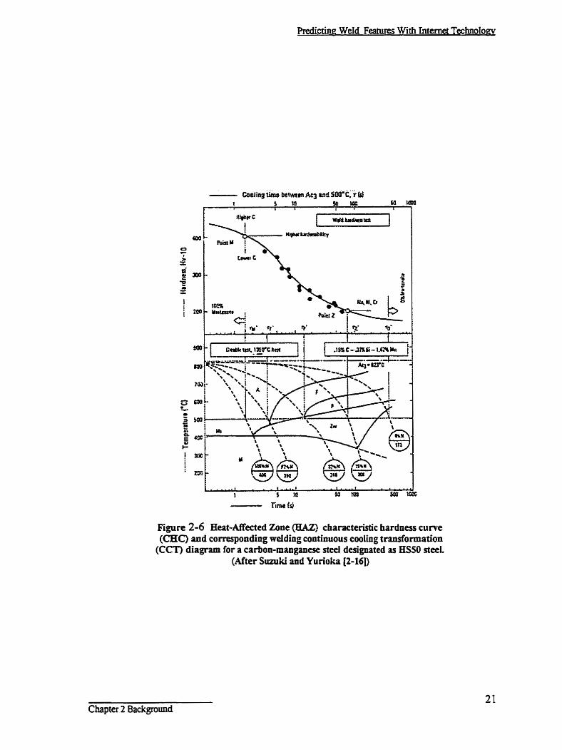
Figure 2.6 shows the HAZ hardness distribution that corresponds to the welding CCT

diagram. Where the cooling time is short, the hardness is high because martensite is expected in

this regime. As the cooiing time increases, bainite andior, femte and pearlite can form, and the

hardness drops. The shape of the hardnessfcooling time curve is characteristic and has been

called the characteristic hardness curve (CHC). Models for predicting HA2 hardness are al[

based on the CHC. The problem reduces to predicting the CHC for a given chemistry and

cooling time.

Predicting WeId Feahues With Internet TechnoIogy

Figure 2-6 Heat-M'cd Zone (HAZ? characteristic hardaess curve (CHQ and corre~ponding welding continuous coolhg transformation

(CCT) diagram for a carbon-manganese steel designated as HS50 steel (After Suaiki and Yurioka [2-161)


Predictina Weld Feanim Wirh Inremet Technology

2.3.2.1 Suzuki Model

Suzuki [2-121 some time ago suggested a backward logistic function to simulate

the CHC as follows:

Equation 2-6

where:

Hm, = the HAZ hardness (W)

& = base metal hardness (WIN)

bs = weld center line 800 to 500 O C cooling time (s)

The comant K is the dzerence between the martensite hardness and base hardness as

s h o w in the Figure 2-7.

Iog (a

Figure 2-7 : Schtmatic diagram to defme the constant K in the Suuiki approach for dculating tFAZ hardnes

K is a function oîcomposition as follows:

K = 169 + 454C - 36Si - 79Mn - 57Cu - lZNi - 53Cr -122M0 - 169Nb -7089B

Equation 2-7

The constanfs &, a and Y are detemined fiom the reiationships:

&=884C+287-K Equation 2-8

aK = 478 + 3364C - 256Si + 66Ni - 408Mo -1321V - 1559Nb Equation 2-9

Y = 4.085 + 2.07C + 0.495% + 0.655Cu + 0.122 Ni+ 0.222 Cr - 0.788 Mo t 30B Equation 2-10

the appropriate weight percentage (w/o) is to be substituted where chernid syrnbois

appear in these equations. The Suzuki relationship is vaiid for low alloy and microalloy

compositions containing carbon in the range as show in Table 2-3.

TaMe 2 3 : Composition Limits for the Suzuki BAZ Hardneu Modd

C hapter 2 Background

[ Alloying Element WtOh range C

1

0.0 17 - 0.33 Si j 0.05 - 0.65 t 1

, M n 1 0.45 - 2.06 1 I

1 CU 1 0.00 - 0.47 I

! Ni / 0.00 - 2.09 I

1 ~r / 0.00 - 1 .O6 1

i Mo / 0.00 - 0.66 d

/ V 1 0.00 - 0.07 j ~b 1 0.00 - 0.06 ! Ti 1 0.00 - 0.02 - - -

1 B 1 0.00 - 0.0023 1

Predictin~ U'eld Features Wirh Intemet fechnolw

23.2.2 Terasaki Mode1 I

Teresaki proposed two independent formulations [2- 13,2- 14 1 to simulate the

C w . The fust mode1 fmulation can be seen as follow-ng:

For ts/5 Iess than or equal to h:

&= 812C + 293 Equation 2- 1 1

For greater than k( :

where

Si Cr Mo H,, =164 C c - + - + - + V + N b + 7 B ( 2 7 2

Equation 2.12

Equation 2- l3

Equation 2-14

log t~ = 2SC, - 1.27 Equation 2- 15

Equation 2-16

where

HvM = hardness of 100% rnartensite (WN)

= hardness of 0% martensite (WIN)

r~ = 800 to 500 O C cooiinp time for 100% martensite transformation (s)

C, = carbon equivalent

This (Table 2-4) is the chernical composition limitation for Terasaki 1 mode!.


Predictin~ WeId Feanires With Internet Technoloev

Table 2-4 Composition Limits for the Tenuici 1 HAZ Hardnas Modd

2.3.2.3 Teresaki Mode1 II

The Tereasaki HAZ hardness equation that approximates the CHC is as

follows:

HV = ( ~ m - ~ v o ) a c p ( - 0 . 0 5 ( t ~ ~ - t ~ ) ~ } + HVO Equation 2- 1 7

Where Hvm is the HAZ hardness corresponding to 100 w/o manensite:

Hm=812C +293

Hvo is the HAZ hardness corresponding to O w/o martensite:

Hvo = 293C + 47Mn + 48Si + 44Cr + 91Mo + 8Ni + 165V +

Equation 2- L 8

95Nb + 794B + 87

Equation 2- 19

The

A =

constants A and t, are evaluated as follows:

5.1C + 1.7Si - 0.39Mn + 0 . m - 1 - 3 0 - 0.8Mo + 6.4V + 3Ni - 45B + 0.29

Equation 2-20

log(t,) = 0.83 ~an(8C)+0.64Mn+0.38M+0.73CrH).76Mo + 0.65Cu + 150B - 1.505

Equation 2-2 1

Chapîer 2 Background

Predictiq Weld Featurcs Wit h Intemet Technoloq

The Teresaki II b i t s are shown in Table 2-5.

Table 2-5: Composition Limits for the Tcmsaki II KAZ Eardnçss Weld Modd

Yurioka proposed two relationships, one for low alloy materials and a second for

Alloying Element C

higher alloy tmnsfonnable steels [2-15,161. At the sarne time Yurioka's formulations

Wt% range 0.04 - 0.26

incorporateci multiple carbon expidents instead of thc single carbon cquivalent foms

proposed by Teresaki and Sund«. - Rie Yurioka relationship forlow-alloy steels

(sometimes cded the Yurioka 1 formulation) is as follows:

Equation 2-22

where:

Cesi = C + Sin4 + Mn16 + Cd15 + NU40 - Mo/4 +VI5 + Nb!5 + IOB + Cr/6

Equation 2-23

CcpnXC-Si/30+Mn/5+Cu/5+Ni/20+Cr/4+Mo/6+10B Equation2-24

The chernical composition limits for the Yurioka 1 mode1 are show in Table 2-6.

Chapter 2 Background;

Predicîin~ Weid Features Wtth Intmet T ~ h n o l w y

Table 2-6: Composition Limits for Y~trioh I W Esrdness WeId Modei

Alloying Element 4

&/O range I

Tl,e first equivdent, CqI, is dominant where the cooling tirnes are long,

. L., CI .-ICI.. .,,A ,-king C)C I~ I - tlU kiC&iess conditions while the second carbon equivalent, Cqn,

dominates in the transition region between the critical cooiing times for 100% and 0%

2.3.2.5 Yurioka Modei II

The second Yurioka mode1 [2-161 was developed for higher alloy transfomiable

steels as show in Table 2-7 below. Aithough transformable higher ailoy materiais are

quite different than the low alloy and microailoy materiais considered in the Suniki and

Teresaki models, i k y are included here because this extends the range of applicability of

the web system which will undoubtedly appeal to usen.

C hapter 2 Backgroundl

Predicting Weld Features With interner Tedinolopu

The formulation for this model is as follows:

Hvmax = 220 + 442~ (1 -0 .3~~ ) + 65tanh y

+[ 68 + 402~(1-0.3e) - 59tanh y] arctan x

Tabk 2-7 : Composition Limitr for Yurioka II EAZ Bnrdness Weid Model

1 Ailoying Element Wtoh range

Equation 2-25

C Si Mn

where:

0.00 - 0.80 ! 0.00 - 1.20 0.00 - 2.00

Equation 2-26

Equation 2-27

I Cu [ Ni

Equation 2-28

CEn = C + Sin4 + Mn/S + Cu/lO + Ni/18 + Cd5 + Mo/2.5 + V/5 + Nb/3

0.00 - 0.90 0.00 - 10.00

CEDI = C p + Md3.6 + Cd20 + Ni/g + Cr/5 + Mo14

where

CE[- IL ui = carbon equivafents

Cp = effective carbon

= C


I Cr , 0.00 - 10.00 +

[ MO 1 0.00 - 2.00

Equation 2-29

Equation 2-30

Predictim Weld Fcatures With htemeî Technoloev

=0,25 + C/6 if C >0.3 wt% Equation 2-3 1

AH = increase in hardenability due to boron for S 5 0.0 16 wt% and 4 5 60 ppm;

AH values are determined fiorn Table 2-8.

fil = (0.02-Nyo.02

where: N is the nitmgen content in percentage weight.

Equation 2-32

Table 218: AX Values Corresponding to Bron Content

Bonn Content (ppm) AH value

While these algorithms are straightforward in pnnciple, it is necessary to code them for

the web based system. As discussed previously the coding syaem selected was the Java applet

technology. Java applets cm be dodoaded fiom a web semer for rernote use. Moreover, they

are relatively platform independent and therefore can be accessed by a wide range of users

2.3.3 Predicting Weld Features

In addition to HAZ hardness, a system for predicting weld shape and size has been

incorporateci into the web system Weld size is an important feature for productivity and

cos issues. It is aiso integrally related to heat-input, microstructure, hardness, strength and


Redictim Weld Feahvcs With Intema Technoloay

toughness [section 2.11. Therefore, a module for predicting weld size and shape should be

helpful to practicing engineers in several ways.

Formulating a fundamentai physics based model for predicting weld size and shape is not

easily achieved since the welding process is very cornplex and not well understood. In particular

the physics of the arc and its interaction with a workpiece is difficuit to characterize. On the

other hand, several semi-empirical models for determining weld size and shape based on

regression techniques are available for the web system. A review of these models is given in

some previous work by Chan [2-171. Based on the Chan review and the need to use a model

where the coding and cornputer requirements are reasonable, the model selected for

impiernentation is that due to Chandel [2-6,7]. While there are models other than those of

Chandel in the literature, this is the only model incorporated in the web system, prirnarily to keep

the size and complexity of the applet system reasonable.

2.3.3.1 Chandel Weld Features Mode1

The Chandel model assumes that the features for GMAW welds cm be described by a

regression relationship of the fonn:

Feume = I O ~ P V V ~ D ~ L ~ Equation 2-33

where 'Feature' is either bead width @W) in mm, bead height (BH) in mm, penetration (Pene) in

min or total fusion area (A) in mm2 and I, V, S, D, L are welding current (amperes), arc voltage

(volts), wire speed (rnmls), electrode diameter (mm) and electrode extension (mm) respectively

as show in Figure 2.8.

Predictinn Weld Features With htemet Technoiogy -

Wefding WeidQeometry: BW = bead width

vo - arc voltage BH bead height Sp - wire travei speed Pene = penetration

1 Le = elextrode extension A i - deposit a r a De = electrade diameter A2 - plate bien area

1 ht - plate thickness A = AL+A2 - Cotai fusion area

Figure 2 4 Schematic diagram to identify the features in the Chandel weid features modeL

The a, b, c, d, e and K in equation 2-33 are constants which depend on electrode

polarity and the shielding gas composition. Weld size and shape are assumed

independent of the chemical composition of the steel which is a reasonable fim

approximation. Weld efficiency is assumed to be constant and is implicitly incorporated

in the relationships, so obtained. The a, b, c, d, e and K values for each feanire are

tabulated in Table 2-9. It should be noted that this regession analysis is really only

valid for GMAW, BOP welds. However, the results of these computations form a

usenil bais for estimating weld size and shape for situations other than BOP.

With the coefficients from Table 2-9, ail of the weld features referred to above

can be calculated, with the exception of the deposit area and the fusion area. However,

Chandel also generated a meIting rate expression for calculating the deposit area:


Pndicîinc Weld Feature~ With Internet Technolcm

where:

I = welding current (Amp)

V - arc voltage (Volt)

D = electrode diameter (mm)

L = electrode extension (mm)

w, x, y, and z are given in Table 2-10

The deposit area A l can be calculateci from the melting rate as follows:

A1 = 35.47*(MR/v)

where:

Equation 2-14

AI = deposited a r a (mm2)

MR = melting rate (k*)

v = mvel speed (mm/s)

It follows that the plate fusion area can be detemhed as die ciifference b e ~ e e n the total

fused area (Table 2- 12a) and the deposit ara:

M = A - A l Equation 2-36

where:

A2 = plate fusion area (mm')

A 1 = deposited area (mm2)

A = total weld bead area (mm')

Redicting Weld F e a m With Intemet Technology

Table 2-9a Coeffiaents for Chandeh Weld Bead Dimension Modeb (C-25 Shiddbg Gas and + ~ e Electrode PoIarity)

Dimension K a b c d e

A -2.350 1.689 0.260 4.850 -0.630 0.253 5

BW -0.218 0.181 0.860 4.614 0.567 0.0106

BH -1382 1.200 -0.690 4.450 - 1.360 0.3800

Pme -4.030 2.050 O. 142 4.530 4.860 -0.0630

Table 2-9b CocffiCcnb for Chandef's Wdd k d Dimcnsion Md& (C-25 Shielding Gts and -ve Elearode Polarity)


A -1.517 1.377 0.271 4.905 4.298 O. 1900

BW -1.500 0.520 0.272 4.570 0.275 0.000 1

BH 4.460 0.690 -0.460 -0.360 -0.660 0.3370

Pene -3.250 1.740 -0.093 -0.366 -0.460 -0.0630

Table 2-9b Coefficients for Chandel's Weld Bead Dimension Modds (M-2 ShieldiapI Gas and +vt Eltctrodc PoiariW)

Dimension K a b c d e A -2,290 1.615 0.202 -0.835 -0.680 0.3400 BW - 1 .O04 0.534 0.660 4.307 0.146 0.0258 BH - 1,440 1.070 4.540 -0.450 -1.370 0.4900 Pene -3.500 0.535 2.610 -0.340 -0.876 -0.6890

Table 2-9d Coeffiaents for Chanders Weid Bead Dimension Models 05-2 Shielding Gas and -ve EIearode Pohrity)


A 4.544 1.123 -0.0378 4.815 0.0320 0.166

BW 4.900 1.030 -0.2300 4.550 -0.0052 O. 128

BH 4.380 0.235 4.0SSO -0.320 4.2070 O. 120

Pene 14.420 1.246 1.8152 4,183 -0.236û 4.567

Table 2-10 Cocffiaent for Chandel's W i n Meiting Rate Equation Shielding Electrode w x Y z Gas - Polari'r

C-25 +ve 0.0230 0.000460 0.000003û6 4-50 C-25 4% 0.0 195 0.000158 0.00000 100 0.39 M-2 +ve 0.0200 0.000540 0~00000 100 4.56 M-2 -ve 0.0268 0.000360 0.00000 100 0.1 1

This completes the background necessary to implement a web based system for

predicting weld features. The Chandel algorithm for determining size and shape is coded

PrcdictiriP Weld Feaîurcs wth Intemet Technolonv,

in tenns of the Java applet system which is housed on a sewer and down loaded by users for

remote processing as needed.

2.4 Com~utational Models for CBPN) Processing

The database available for regresion purposes and the number of parameters used in

the d y s i s usually limits the applicability of the analysis. -4s a renilt, tle final mcdel c3n

be limited if new sensitive panuneters are found in later study. Since regression methods are

essentially a w e W n g technique, it becomes difficult to modie the finai model by adding

or reducing parameten or by changing the limits of the data Usually, modieing a

regression expression requires restamng the analysis as a new problem. As a result, creating

a model can be time consuming and the effective life cycle can be relatively short. In

principle, the back propagation network (BPN) technique, does not suffer the Iimitations of

regression analyses. BPN can identi@ and map both trends and relationships between input

and output data with relative ease even when these relationships are relatively wmplex (i.e.

when there are many factors involved).

This propetty is usefi11 for modeling the welding process to predict HAZ hardness, or

weld size and shape because, among other things, several input parameters (voltage, current,

welding speed, plate thickness, and chernical composition, etc.) are necessary to provide an

unequivocal characterization of the process. In addition inputhutput relationships may be

non-linear and this tw can create uncertainty in either regression or physical modeling. In

principle the BPN rnapping process can deal wit h multiple input/output parameters and non-

linear relationships.


Predictintz Weld Features With Imemer Techwlopl 1

Figure 2-9 Basic ANN structure.

2.4.1 Back~ropagation Network (BPN)

The basic concepts of the BPN method are captured fiom the mechanism that is

thought to controi the biological nervous system. In pnnciple it seems to be a relatively

simple mechanism that can be simulated by cornputer to solve complex physical

probIems. A general artificial neural network (ANN) consists of a series of weighted

nodes connected together in a manner that simulates biological neurons. Usuaiiy, the

nodes are arranged to have a layered structure- There are interlayer nodal comec tions

but no nodal connections within Iayen. A typical structure consisting of an input Iayer, a

hidden Iayer, and an output Iayer is shown in Figure 2-9. The input layer accepts

information (e-g welding parameters) whife the output layer yields calculated results


Redictinn Weld F e a m With Intemec Technology

nich as HAZ hardness, cooling time a d o r weld feahres. Hidden nodes and layers

constihite the intemai representation of the network Information is manipulated

intemally to identity and fix the trends and relationships that exist between the input and

output data. Thus, the number of hidden layers and the number of nodes in each layer are

adjusted to reflect the nature of the problem at hand. Basically the number of nodes and

layers depends on the complexity of the problem.

AIthough a BPN network can achieve complex tasks with a combination of nodes,

a single node has two simple functions: nimation and transfer as shown in Figure 2.10.

With summation ail incorning weighted signais, that reflect nodal activity, are combined.

Mathematically summation for the hidden nodes is expressed as follows:

L - summioa lundioa F- Lransler_ri?ndron

Figure L1D Single node function.

where :

Equation 2-3 7

Si = surn at the ith node

= incoming signal from the h* node


W, = weight between the hUL node and i* node

The outgoing signal depends on both the summation resuit (S) and the transfer

function (F) used for this purpose. Any one of several transfer functions could be used -

such as a step function, a ramp funaion, a sigrnoidal funaion. S-shaped curves, etc. The

sigrnoidal bct ion was selected for this study because, among other things, both the

function and its derivative are continuous, which is similar to the response of biological

neurons. It has the form:

Equation 2-38

With summation the weights are adjusted for each link and the input signais are

thereby converted into output signais. In theory, there is a set of weights that custom

tailon the system so that it will respond correctiy in a specific domain for each problem.

The search for the correct set of weights (specific to each problem) is called

network training or learning. It is necessary to have a training data set (usually

experimental data) frorn which the network acquires knowledge. It is important to select

the training data set so that it cuven the entire domain of the problem. For example,

maximum and minimum &ta should be included in the training selection.

In addition to the training data it is important to have a test data set which can be

used to ven@ the integrity of the system. Usually, any expenmentd data that is not

selected as training data set becomes test data In this thesis, the expenmental database

consisteci of HAZ hardness values or weid size and shape parameters, as the case may be

against the corresponding welding parameters - voltage, current, welding speed, etc. In

each case, generaiiy, about 20-30 measured HAZ hardnesses (or weld sjzes and shapes)

are selected h m the database of up to 100 sets to train the system.

The training method used in this thesis is 'kror backpropagation" [2- 181. The

principle is to optimize its weight set so that differences (enon) between the original

experirnental data set and the corresponding output dat3 set h m the BPN are minimizzd

In detail, the error (E) is found by making use of the least square method:

which basicai 1 y reflects the ciifference between the network output signal (O") and the

corresponding target output signal (Ot) from the training data set Once this difference

reaches an acceptable to lemce level by changing weights in the network, the Iearning is

said to be complete.

Chapter 2 Backgound

Pdictinn Weld Features With intemet Technology

1 I I l

hput Signals

Weighted Weightd Links (Wi) Links (Mj)

inpm Layer HiddenLayer Ourput Layer (hi (9 Ci)

Figure 2.11 A bickpmpqation network

The enor backpropagation Iearning process can be seen in Figure 2.1 1. Fint, w e i g h

between the last hidden layer (next to the output layer) and the output layer are adjusted

initially based on the enor found from Equation 2-39. Then the weights in the next to the l a s

hidden layer are adjusted and so on until the input layer is reached. In other words weld

predictions are cmied out in a forward direction, while weight adjustments are propagated

back through the syaem (Figure 2.1 1). Bias nodes (B) [1-18, 191 are extra nodes that have

been added to every layer except for the output layer as shown in Figure 2.1 1. The purpose of

this is to stabilize the training process by providing an intemal reference for each layer.


Predicting Weld Features With Internet Technology

The weights connecting the output layer and the last hidden Iayer are adj usted in

the following way:

AYj = q I J , +a A W ~ Equation 240

where: q = the l e d g rate

fi =hidden layer node

6j = delta tenn (mount to be changed bas4 on the error obtained)

i = hidden layer node index

j = output layer node index

a = momentum coefficient (value between O and 1)

~lir-' = weight adjustment tem fiom prerious p3th

The leaming process is tnggered by the delta terni, which is based on the error detected

according to:

6, = F(S, X1- F(S,)XOt - O n ) Equation 3 4 1

From Equatian 240 and 41, those weightq are adjusted based on the delta terni

(6), the lezving rate (q) aod the mornentum coefficient (a). The Ieaming rate (q) a n be

viewed as the step sire in the search for the optimum weight set, thus learning can be

accelerated or decreased by adjusting the leaming rate. However, the learning rate m u t

be cansidered carefully hecause the desired weight set may be missed if the step size (Le.

leaning rate) is set tao large. On the other hand the whole search process becomes slow if

the Ieaming rate parameter is set too low. Figure 2-12 shows a simplified weight-

error relationship for training From this figure, the learning rate has significant influence


on the ske of the width, which is Iabeled as

"change of weight". The momentum

parameter is used so that the search is

not trapped by a local minimum as shown

in Figure 2-12. Because of the nature

of the leaming rate and the momentun

coefficient, they should have positive

values between O and 1 [2- 181.

Figure 2-12 Simplifiai network weight - e m r niationsiiip.

Errors are backpropagated to refine the weights comecting the input and hidden

Equation 2-42

It should be noted that the delta equation, Equation 2-42, is different from the previous

one, Equation 240. This is because the weight adjuaments for an input-hidden layers

involves a previous layer (hidden-out layer, in this case).

After the first pattern (set of data) has been mbmitted to the network, the weights

nd rd are adjusted accordingIy as documented above. Thereafter the 2 , 3 , and al1 other sets

(up to the Ph pattern) are submitted to the network and after each submission, the

weights are adjusted. A complete set of patterns (data sets) submitted to the network

during learning is said to be an "epochn. Usually many epochs are necessary for learning

Chaptcr 2 Background 41

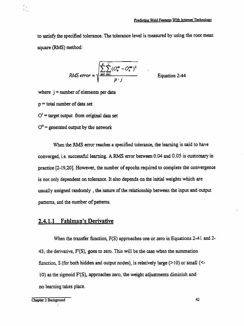
to sa&@ the specined tolerance. The tolerance level is measured by using the root mean

square (RMS) method:

Equaîion 2-44

where j = amber of elanents per data

p = total number of clata set

0' = target output tiom original data set

O" = generated output by the network

When the RMS error reaches a specified tolerance, the learning is said to have

converged, Le. successful learning. A R h 6 error between 0.04 and 0.05 is customary in

practice [2-19,201. However, the number of epochs required to complete the convergence

is not only dependent on tolerance. It also depends on the initiai weights which are

usually assigned randomly , the nature of the relationship between the input and output

patterns, and the number of patterns.

When the transfer fiindon, F(S) approaches one or zero in Equations 2-41 and 2-

43, the derivative, F(S), goes to zero. This d l be the case when the summation

funnion, S (for both hidden and output nodes), is relatively large (X 0) or smdl (c-

10) as the sigmoid F(S), approaches zero, the weight adjustments dùninish and

no learning takes place.

Fahlman [2-211 proposeci a slight adjustment to the derivative of the sigrnoid

function, Equation 2-38, by adding 0.1 to the equation:

F1(s )4 . 1 + [ l -F(S) ]F(S) Equation 2-45

The modified value, 0.1, is arbitrary selected, but it is important to keep the network

leaming. In the original code Fahiman's derivative was applied only to the hidden-output

layer. However, Chan et al [2-221 suggea that the modified derivative should be applied

to al1 layers.

2.4.1.2 Other Issues with the Bacbro~agation Network

In addition to the basic mathematics and enhancements of the backpropagation

network, there are some other considerations for applying the network to real practical

service. Ail input and output data are n o d i z e d between the upper and lower

boundaries The selection of limits is important for the se~ceabili ty of a production

shed network. Since the transfer function is limited to the range between zero and one,

the network output is also limited to this range. Because of this, extrapolation beyond the

upper and lower limits is not possible. Therefore, it is necessary to do normalization

before training aarts. Moreover, if the range of the upper and Iower limits is set too

narrowly, the applicability of the network will be limited. On the other hand, if the range

is set too wide, the network near the limits becomes unreliable. In this application, the

output will be one or zero if the sumation, S, approaches positive and negative infinity

respectively for the sigmoid tramfer function. Therefore, the maximum and minimum

Predicth Weld Features With Internet Technology

data are normalized to 0.05 and 0.95 of the span respectively. Changing the range may

also improve the leaming time and accuracy of the network prediction.

2.4.2 BPN HAZ Hardness Model

The HAZ hardness BPN mode1 used for the web system in this investigation was

first established by Chan [2-221. The input parameters for this system are the 8 0 0 ~ ~ to

5 0 0 ~ ~ cooling time, t&, the carbon content (wfo) and the carbon equivalents (Pcm

proposed by Ito and Bessyo[2-231, and CE attributed to Yunoka and Suniki [2-241):

Equation 2-46

Equation 2-47

As discusseû in Section 2.2, a carbon equivalent refiects the hardenability of a steel.

In principle hardenability could be accounted for by considering each element

individually as an input parameter. However, the complexity of the network increases

considerably with each parameter added to the input nodes as the relationships in section

2.4.1 would indicate. In fact, with a relatively complete analysis for a typical low alloy

steel of some 10-12 elements, the network complexity becomes unreasonable. Therefore

some combination of elements is necessary to sirnpliQ this problem. Several carbon

equivalents have been suggested in the literature but CE and Pcm are those most widely

accepted with regard to cold cracking. Since there is a relationship between H M

hardness and cold cracking, it is not unreasonable to use these same w b o n equivalents

for the web based hardness system. Indeed this was the philosophy used by Swuki who

proposed two HAZ hardness formulations NSC-S (CE) and NSC-S (Pcm) in an effort to

-- - .-


Prediaing Wefd Features With Internet TechnoIo=

uni@ cold cracking and HAZ hardness technology[Z- 121. Both carbon equivalents are

included because it is said that Pcm is supenor to CE when the cooling duration is

relatively short, while CE is a better representation where cooling times are relatively

long. Moreover, it is well known that Pcm correlates better with the cracking behavior of

rnicroalloy steels and low alloy steels with carbon content less than 0.17 wfo while CE

correlates better for carbon levels in excess of 0.17 w/o [2-121. By including both carbon

equivalents, the BPN system uses them both during training to correlate input with output

as appropriate.

Carbon content is also incorporated separately since it essentially detemiines the

hardness of martensite as discussed in section 2.2, in addition to its hardenability role

refleaed through the carbon equivaient formulations. The cooling time reflects the

welding parameters (Le., arc curent, voltage, travel speed, and plate thickness) and their

effea on HAZ hardness. It is worth noting that the coolhg time is determined by a

separate neural network where the input parameters are the welding conditions.

By combining the two BPN models (one for tas, and one for HAZ hardness), the

HAZ hardness can be prediaed in VHN. Chan found that the most successfil BPN

configuration for the KAZ hardness problem was two hidden layers with 5 and 3 nodes

(including bias nodes) and a single hidden layer with 4 hidden nodes (including a bias

node) for cooling time respectively. Therefore these same configurations were used for

the web based mode1 in this investigation.


2.4.3 BPN WeId Features Mode1

Chan [2-221 also developed a BPN system for predicting weld features which is

incorporated into the web system. The input parameten are welding voltage, current,

welding speed, plate thickness, process eficiency and gas cover (M-2 or C-25). The

fusion area, which is similar to the one for the Chandel weld feahire mode1 (section

2 . 3 . ) In addition a new parameter was introduced, called bay length. The new

parameter reflects the unique shape in the plate fusion area (Figure 2.13) for deep

petration welds. The region where the weld m o w s is called the bay area It has k e n

found that, quite by accident, the natural bay angle seems to be about d8 (22.5 degrees)

and it is therefore only necessary to determine the length by BPN means [ 2-81.

P

I lower-bead plate \laver-bead bay angie ' ' fusion , bay length

area ,,/

Figure 2-13 Wdd bead modd cross section with bay Iength and angle definition.

A parabolic cuve has been used to represent the deposited area from the predicted

parameten, bead width (BW) and bead height (BH) :

y = - & c b Equation 248

where:


b=BH Equation 2-50

Two intenecting parabolic curves are used to represent the plate fusion shape in

tems of the parameters, penetration, bead width and bay length The bay length is used

to fix the intersection of the two curves [2-221. The top part of the shape is expressed in

terins of one parabola as follows:

Y' = c(x+d) Equation 2-5 1

while the lower part takes the form of the other parabolic expression:

y = ex' -f Equation 2-52

where:

Equation 2-53

d = BW/2 Equation 2-54

Equation 2-55

f = Pene Equation 2-56

xi, y1 is the point of intersection of the two parabolas which is determined fiom the

following:

Equation 2-57

Equation 2-58

where i = bay length (mm)


Predictina Weid Features Wah Interne Technologv

From these equations, a computer generated pictorial shape of a GMAW weld is

possible. Chan found that the weld shape subsequently generated by BPN and presented

in terms of parabolic curves represents the GMAW welding process quite well. Such a

system is undoubtedly usefid to welding engineen in practice. The next step in the

development of computer tools for welding and manufacturing engineen is to ma! this

software widely available by modifymg it for use on the world wide web system as

discussed previously.

2.5 A Web Based Internet uWeidsoft" Svstem

As described above, Chan [2-17,221 developed a usefùl regression software

systern on the one hand, and a BPN software system on the other, for predicting cooling

times b s , HA2 hardnesses and weld features (size and shape) from the input welding

parameters for the GMAW process. The Chan software systern is one of the first

comprehensive cornputer tool sets for engineers who must specify welding procedures

and conditions in practike. It is easy to demonstrate that this system can save both time

and money because, arnong other things, the weld size and shape parameters are

productivity issues and HM hardness is a weld quality indicator.

The Chan system is knom to be quite usehl for those in the reseanh community

who read and follow such weld process developments. Moreover, a commercial version

of the system is marketed by the American Weiding Society, among othen. Yet with

rapidly increasing use of the Intemet, it has been suggested that this would be a way of

bringing this software to the attention of a greatiy expanded audience of welding and

fabrication engineers.

. - -- -


P r e d i h Weld Features With Intemet Technolw

While everyone is aware of the Internet, it is worth a brief description of how it

may be used in the context of the web system described above, It is well understood that

the Intemet rnay be viewed in its simplest fom as a network of cornputers comected

generally by telephone lines or by some other means of electronic communication. If the

"weldsoft" system is made available on a "server", then in principle, anyone, anywhere

with a computer connected to the Intemet can access it. Moreover, since the software is

hosted on a server, upgraduig would be &ed out centraily, and from a user point of

view, hdshe is always using the most updated version of the software. For exarnple, such

a systern could be housed on the Cambridge University server available through the

courtesy of Professor K Bhadeshia, Department of Materials Science, for this purpose

[2-251. There are, however, significant computer issues that must be addressed before this

can be realized.

The Intemet world wide web (WWW) is a standardized method of publishing

information on the Intemet, using a computer language calleci the Hyper Text Markup

Language (HTML). When the location of the desired information is known the-address in

the f o m of a Universal Resource Location (UN,), is submitted to a browser (Netscape or

Explorer), which in tum reaches out to access the server. Once the comection is

established, information is retumed in HTML form, and decoded by the browser.

Java is another comput er language designed for Intemet applications. This

language has more functionality than HTML. It is capable of traditionai computer

processing such as calculations and graphies, while IiTML is lirnited to text

Predictin~ WeId Features With Intemet Technoloey

enhancements of one sort or another. Moreover, s d l e d applets can be creaîed with

Java. Essentially the Java operating system is transmitted with the application in applet

fom to the user's cornputer. In this way the system is more or less plaaorm independent

and an applet c m be customized with instructions to provide great flexibility.

In this thesis applets for calculating K4Z hardness and wdd fean~es arc

presented The fifit system consists of applets based on the regression relationships

detailed above. A second system is based on a BPN system first established by Chan It

consists of applets pre-aained to calculate HAZ hardness and weld features. This

might seem like duplication especially since the accuracy and range of applicability of

both systems is similar. However, there is considerable uncertainly when doing

calculations which are regression or neural network based and the redundancy offered by

the two systems is useful for the practitioner. It provides confidence if both systems are

in reasonable agreement or a waming if they are not in agreement.

Whle the Java applet software tools for the welding process represents a

considerable step forward, a third untrained BPN system is proposed Like the previous

BPN systern it is designed to caicuiate HAZ hardness and weld features, but unlike the

previous system processing is to take place on the server. Essentially it wodd permit

"custom training" by users who wouid submit training data As discussed previously

welding practice is not entirely universal and there are differences in the industry based

on traditions and expen'ences. Many of these can be captured with custom training and

therefore providing an untrained web based system will undoubtedly be use hl to the

welding commUNty.


Predictinsz Weld Featutes Wih interna Technoloq

But over and above the training issue, a server system would permit capturing

user details and their training data A database of users and training data would serve the

welding and engineering communities well. Arnong other things it could well encourage

"electronic" collaborations on a large scale by providing access to a large database of

experience and sofhMTe tools for processing. However, ananging for data capture md

processing on a server gives nse to several as yet unanswered research issues. A

description of the system and a discussion of the issues is included in the foilowing

sections.


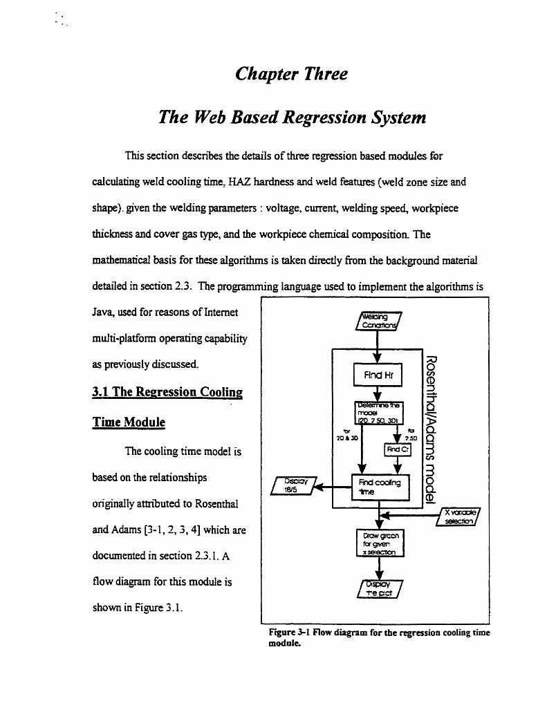
Chqter Three

The Web Based Regression System

This section describes the details of three regression based modules fOr

calculating weld cooling hme; HAZ hardness and weld fattues (weld zone sie and

shape). given the welding parameten : voltage, curent, welding speed, workpiece

thichess and cover gas type, and the workpiece chemical composition The

mathematical bais for these dgorithms is taken directly fiom the background material

detailed in section 2.3. The progmmming language used to implement the algorithms is

Java, used for reasons of Intemet

multi-platforni operating capability

as previously discussed.

3.1 The Regression Coolinp:

Time Module

The cooling time mode! is

based on the relationships

originally attncbuted to Rosenthal

and Adams [3- 1 , t , 3,4] which are

documented in section 2.3.1. A

flow diagram for this module is

show in Figure 3.1.

figure 3-L Flow diagram for the mgrasion cooling tirne modale,

Predictins Weld Feahlres with Internet Technoloq

The welding parame ters (voltage, cwent, travel speed, process e fficienc y,

ambient temperature and wotkpiece

thickness) are subrnitted to the

cooling time module. The energy

input is first cdcdated accordine to

equation 24. The energy input is

multiplied by a process efficiency

to generaîe a heat input (J/mm) and

this together with workpiece

thickness is used to determine the

heat flow regime (2D, 2.5D or 3D)

figure 3-2 User interface for the regnuion cooling time module

according to equation 2-5 as discussed in section 2.3.1. With this decision in hanci, the

cooling time is then caiculated with one of the 2D,

2.5D or 3D relationships (equations 2-1,2-2 or 2-3),

whichever is appropriate.

Mile the calculation is straïghtfonvard in

principle, user convenience is an important

consideration. In this regard a convenient user

interface has also k e n generated using the Java

program language as shown in Figure 3-2. It consists

of three separate work areas. The welding parameten Figure $3 la put area for the regression cooiiag tirnc,

Chapter 3 Web B a d Rewnion Model

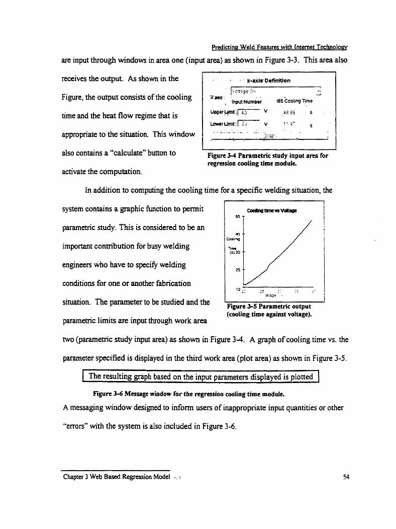
Predicting Weld Feamm with [ntemet Technoloa

are input through windows in area one (input area) as shown in Figure 3-3. This area also

receives the output As shown in the

Figure, the output consists of the cooling

time and the heat flow regime that is

appropriate to the situation This window

also contains a "caiculate" button to I Figure 3-4 Pammetric study input a m for I regttssion coohg tirne module

activate the computation.

In addition to computing the cooling time for a specific welding situation, the

system contains a graphic fiinction to permit

parametric midy. This is considered to be an

important contribution for busy welding

engineea who have to specify welding

conditions for one or another fabncation

situation. The parameter to be studied and the

parametic limits are input through work area

L

Figure 3-5 Parametrie output (cooling time against voltage).

parameter specified is displayed in the thxrd work area (plot area) as shown in Figure 3-5.

1 The resulting graph based on the input parameters displayed is plotted 1 Figure 3-6 Masage window for the rcgression eoaling time module

A messaging window designed to infom users of inappropriate input quantities or other

"errors" with the system is also included in Figure 3-6.

Chapter 3 Web Based Regmion Mode1 -.:

rnctine WeId Features with internet Technalogv

3.1.1 Verification of the Rwression Cooling Time Module

To test the validity of this module, calculated data have been compared with

experimental data as shown in Figure 3-7. The experimental data used for this purpose

were taken from the research of Kohno [3-51- 25 submerged arc welds, the work of

Yunoka 13-61 - 9 shieldd metal arc wdds, and the researth of Signes 12-71 - 56 gas

metal arc welds.

It is apparent that the calculated values for mling time for the range between O to

60 seconds are reasonably accurate or at least in reasonable agreement with rneasured

values. However, the calculated values dnft considerably high when the measured values

exceed this value (60-200 seconds). This is not a serious limitation because situations

where the cooling times exceed 60 seconds are large welds where there is little W

hardening. Therefore crack formation due to HAZ hardening is not normally a problem in

this range. Moreover, large pass welds using a technique like the submerged arc process

are much less common than smaller multipass joints using a technique Iike the gas

shielded metal arc process. Nonetheless, the experience of this investigation suggests that

the web based cooling time software should be limited to cooling M e s of 60 seconds or

less.

It is intereshg to speculate why the calculated cooling times are higher than the

measu~ed values for larger welds. In fact Figure 3-7 (A) would suggest that at 200 seconds

(measured), the calculated time is nearly three time that at about 600 seconds. The difficulty

is almost certainiy due to the importance of workpiece radiation and wnvective tosses in the

neighborhood of the joint when the heat input is high. The Adams relationships used

Chapter 3 Web B a d Regession Mode1 55

Predicting Weld Feahires with hternet Tectuiolo~

in this software assumes conductive heat transfer only, which seems valid for cooling

times of 60 seconds or less. However it would seem that a mode1 that indudes radiation

heat tramfer would have to be used for cooling tirnes greater than 60 seconds.

Chapter 3 Web Based Regrcssion M d

Predictin~ WeId Feahires with Intemer Technolopy

Cooling Time Comparison Up to 200 seconds

Experirnental values (s)

Figure 3-7 (A)

Cooling Tirne Comparison Up to 60 seconds

Figure 3-7 (B)

Figure 3-7 Cornparison of caicuhted cooiing tirna (Adams mode! cooüng tinte estimation) with m e n s u d vaiua: (A) O - 200 sema& rangc, (B) O - 60 seconds range)

Chapter 3 Web Based Etegession Mode[

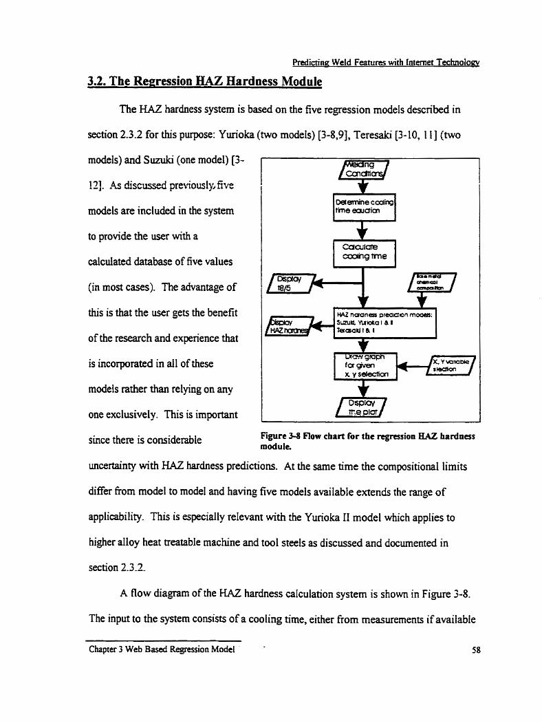
Predinin~ Weld Features with Intemet Technoloq

3.2. The Regression HA2 Hardness Module

The HAZ hardness system is based on the £ive regression models described in

section 2.3.2 for this purpose: Yurioka (two models) [3-8,9], Teresaki [3- 10, 1 1 ] (two

models) and Suniki (one model) [3-

1 21. As d i s c ~ e d preriously, five

models are included in the systern

to provide the user with a

calculated database of five values

(in moa cases). The advantage of

this is that the user gets the benefit

of the research and experience that

is incorporated in dl of these

models rather than relying on any

one exclusively. This is important

since there is considerable Figure 3-8 Flow chart for the rrgrrrsion BAZ bardnesr module,

uncertainty with HAZ hardness predictions. At the same time the compositional limits

differ from mode1 to mode1 and having five models available extends the range of

applicability. This is especially relevant with the Yurioka II model which applies to

higher alloy heat treatable machine and tool steels as discussed and documented in

section 2.3 -2-

A fiow diagrcim of the KAZ hardness calculation system is shown in Figure 3-8.

The input to the system consists of a cooiing time, either from measurements if avaiiable

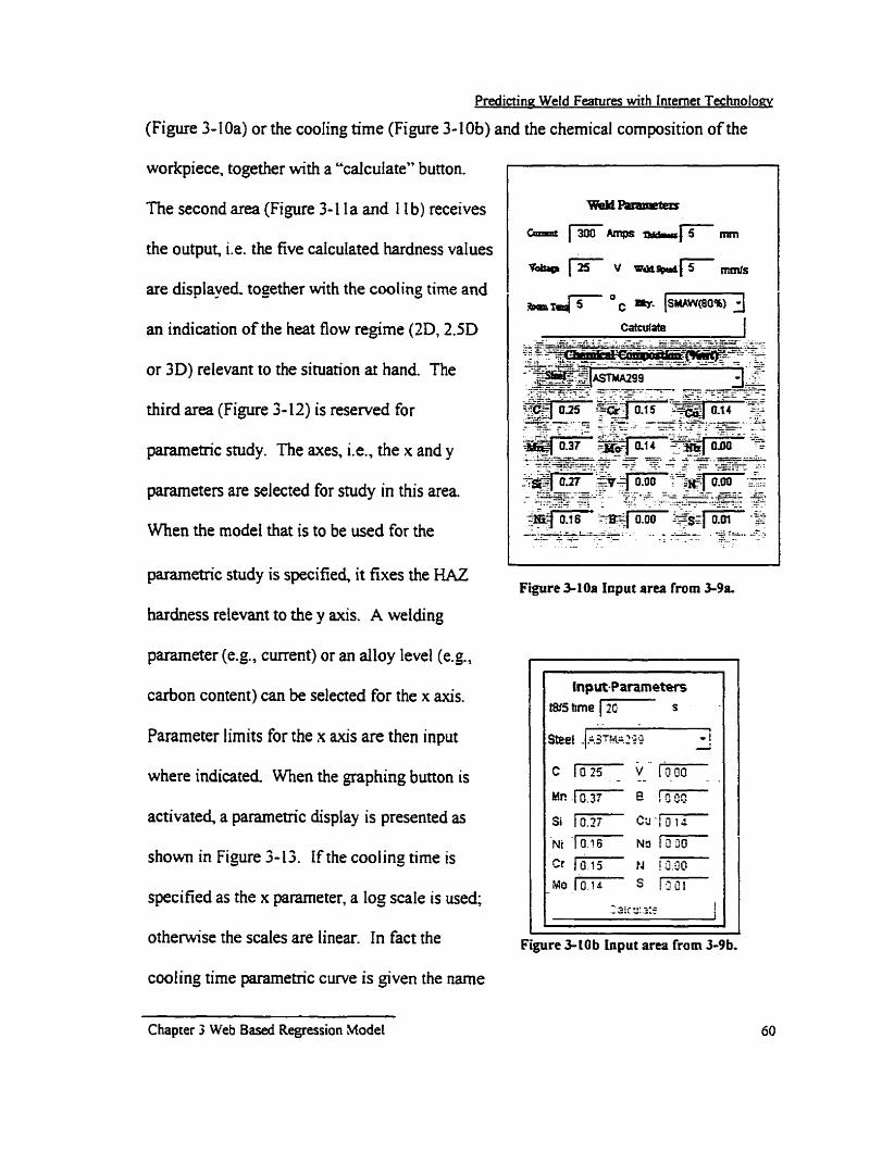
Predictinp Weld Features with Internet Technology

(Figure 3-1 Oa) or the cooling time (Figure 3- 1 Ob) and the chernical composition of the

workpiece, together wiîh a "calculate" bunon.

The second area (Figure 3- 1 1 a and I 1 b) receives

the output, i.e. the five calculated hardness values

are dis~laved . - together with the cooling time and

an indication of the heat flow regime (2D, 2.SD

or 3D) relevant to the situation at hand. The

third area (Figure 3- L 2) is reserved for

parametric snidy. The axes, i-e., the x and y

parameten are selected for study in this area.

When the mode1 that is to be used for the

parametric study is specified, it fixes the HAZ

hardness relevant to the y axis. A welding

pariuneter (e.g., current) or an alloy level (e.g.,

carbon content) can be selected for the x axis.

Parameter limits for the x axis are then input

where indicated When the graphing button is

activated, a pararnetric display is presented as

shown in Figure 3- 13. If the cool ing time is

specified as the x parameter, a log scale is used;

otherwise the scales are linear. In fact the

cooiing tirne parametnc curve is given the narne

Figure S10a Input area from 3-9%

Input-Parameters -1

I - - - -

Figure S E O b input arta from 3-9b.

Chapter 3 Web Based Regression Modet

Ptedicting Weld Features with Internet Technoiogy

"Characteristic Hardness Curve" (CHC), a

concept that was discussed in the background

section 2-3.2.

With this system, welding parameten

and workpiece chernical composition cm be

selecred for any given welding situation. Thus,

ultimately, it is possible to estixnate the

optimum combination of workpiece chernicd

composition and input welding parameters, or

Hardness Preàlatïon in VHN

'Yuhoka t TemsaM I SuaiM

254.9? 234.98 245.82

yurioka I I terasaid I I 21 9.43 21 5.64

Figure 3-1 1 b Résulu area from 3-9b.

at the very least the software provides some reference data for specifying the welding

conditions.

I

F'iure 3-12 Parametric study input area for the regremion BAZ hardncss modules.

Figure 3-13 Hotting a n a for the regression BAZ hardness modules (a CHC is shown).

3.2.1 Verification of the Regression HAZ Hardness Module

To test the vdidity of the HAZ hardness module, calcdated data have been

compared with experimental data as shown in Figures 3-14. The experimentai data used

for this purpose were taken fiom an AMCA research report [3- 131. The c hemical

- - -

Chapter 3 Web Based Regression Model

Predicting Weld Features with hternet technolom

compositions and welding conditions for three different microalloy steels are given in Appendk

II. The carôon content of the microdoy steels mged nom 0.05 to 0.12 w/o, and the IIW and

Ito's carbon equivalents ranged from 0.405 to 0.448 and 0.200 to 0.247 respectively. The

correlation factors, the average value of absolute merence between rneasued and generated

values, and standard deviations of the ciifferences are ail containecl in Table 3-1. These three

factors describe the characteristics of the data distribution. Generaliy, it is apparent from Figure

3-14 and Table 3-1 that there is reasonably good agreement between the measured and calculated

values for a i i models for these particular sieels.

Chapter 3 Web Based RcgéESIon Modd

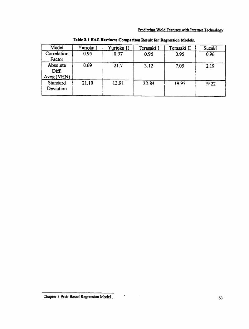
Predicrine Weld Featum with Imernet Technoloqy

Table 3-1 KAZ 8.rdnar Cornparison RauIt for Reerruion Moddr -

- -

Chapter 3 yeb Based Regression Model

Mode1 Correlation

Factor Absolute

Diff. Aveg. (VHN)

Standard Deviation

Yurioka1 0.95

0.69

l

21.10

Yurioka II 0.97

21.7

13.9 t 22.84

t l

19.97 1 9.22 i

Terasaki 1 0.96

3.12

Terasaki II 0.95

Suniki 0.96

7.05 1 2.19 I

Figure 3-14 (b)

= = X O m G Q

-Y*urrmI

Figrire 3-14 (c)

Figure 3-14 Cornparison of rner~ored ( M C A investigation) with dcuiatcd E U hardness : (a) Yurioka L, (b) Yunoka IL (e) Temaki I (cf) TerasaLi Q, (e) Smuki.

Chapter3 Web Based Regression Mode1

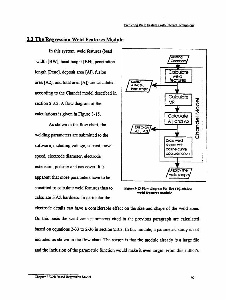
Predictmp: Weld Feahués with intemd Techology

3.3 The Regression Weld Features Module

In this system, weld features (bead

width PWJ, bead height [BII], penetration

length pene], deposit area [Al], &sion

area [A2], and total a m i [A]) are dculated

according to the Chandel mode1 described in

section 2.3.3. A flow diagram of the

calculations is given in Figure 3- 1 5.

As shown in the flow chart, the

welding parameters are submitted to the

software, including voltage, men t , travel

speed, electrode diameter, electrode

extension, polarity and gas cuver. It is

apparent that more parameters have to be

specified to calculate weld features than to

calculate HAZ hardness. In particular the

Calculate 2l

Wd shape /"""/ Fïgurr 3-15 Flow diagmm for the regression

weld featurea module

electrode details can have a considerable effect on the size and shape of the weld zone.

On this bais the weld zone parameters cited in the previous paragraph are caiculated

based on equaticns 2-33 to 2-36 in seaion 2.3 -3. In this module, a parametric study is not

included as shown in the flow chart. The reason is that the module already is a large file

and the inclusion of the parametric function would make it even Iarger. From this author's

Chapta 3 Web Basxi RegtesSon Mode1

Predictina Weld Features with lnternet Technology

experience, an applet file of more than 30K bytes is problematic because among other

things of the limitation of a 56K modem. Currentiy its file size reached 3 1K bytes,

rhus the parametric hction has not been included.

The user interface for this module is 7 1 I-LzZF- shown in Figure 3-14. Similar to the other

T U m t r p r i a l -

user interfaces descnibed previousl y for àic"m/'59

managing the cooling tirne and HA2

hardness calculations, there are three work

areas. The first consists of windows to input 1 . cbir

- -

the welding parameter% t"gether lMith a draw figure 3-L6 User iatulsiee for the regrrrsioi wdd features module.

button (Figure 3- 1 7). The second receives the calculated

weld features (Figure 3-1 8) and the third is reserved for a

presentation o f the approlcimate sbape of the weld based

on the cdculated parameters (Figure 3- 19). The

approximate shape is drawn by judiciously fitting a semi-

ellipse for the upper-bead (deposited area) and a cosine

curve for the lower-bead (fusion area) [3-15, 16, 171. The

validity of this has been shown in the work presented by

Chan [3-141. Figure $17 Input area for the tegrasion wdd features module.

Weld features calcuiatioas and pictorial presentations are expected to be

usefbi for practicing welding engineen. Arnong other things, weld area can be a

productivity parameter. Welding is usually one of the cost-effective joining methods and

Chapter 3 Web Based Regression Mode1 66

Predictina Weld Fearures with Intemet Tahnoloq

Figure 3-1 8 Output area for the regression wdd fa tuns rnoduk

the largest weld area possible would seem to be a logical objective. However, there are

rnany considerations that limit this objective. For example the weld must be consistent

with the joint size and preparation. In addition weld shape can sometirnes give rise to

serious stress concentration problems. There are many such considerations for which the

weld features module can be helpful.

3.3.1 Verification of the Regression Weld Features Module

To test the vaiidity of the weld features module, data provided from the

experimental investigation conducted at Northem College [3- 191 for C25 and M2 cover

gases were selected Caiculated values are plotteO âgîiiist rfieasured vaiues for each weld

feature in Figures 3-20 and 3-2 ! for C25 and M2 cover gas respectively.

It is apparent that there are significant differences between the calculated and

measured values. In general the caiculated deposit and fusion areas are considerably

larger than the measured values. At the same Sme dculated bead width and penetration

are considerably less than measured. At first glance this may seem surprising, but it is

likely explained by the contention that the welding process is very dificuit to controi

precisely enough to generate a univenal regression expression for weld fames. It is

Chapter 3 Web B a d Regression Model

8

postulateci that digerences in welding tradition and ski11 between the Chandel and the Northem

Coliege investigations could account for the difrences observed. In this regard, the BPN system

desdbed in section 2.4 is likely a better method to use for determining weld features.

3.4 Cornputer Reauirements for the Web Based Remession Svstem

The prirnary cornputer consideration when creating a Java based system for the Intemet is

that users must have considerable workstation wmputational power. As discussed previousl y

the primary advantage of a Java based system is that it is designed to mn with several different

operating systems (windows, uni& the apple system, etc.). This is only possible because a Java

code interpreter, necessary to decode a prograrn, is located in the user's Java-enabled browser.

Because of this extra step, the client's machine mua have enough additional computational

power to execute the Java program. At this point in time, the minimum requirement for ninning

the Intemet software described in this thesis is a Pentium CPU processor with 32Mb RAM.

To run the web based system describeci in this thesis, the user machine must have a Java

interpreter or a Java V i a 1 Machine (version 1.1.5 compatible), JVM, installed. MS Intemet

Explorer 4, Netscape 4 or later versions are the most curnmonl y used Java 1.1.5 compatible

NM. Nahirally, if the version of the Java program is more recent than the local Java interpreter

(Le. the user's NM is outdated), it (the interpreter) is not able to convert the Java code for the

operating system, which means that the prograrn cannot be executed at the local site. Version

compatibility can be easily checked; for example a menu cdled "Java Console7' in Netscape

contains the Java version numbers to be checked.

Cbapter 3 Web Based Regression Mode1

Bcad Hught Compahsn for C25 Shielding Oas

lcrin~ Weld Features with bternet Technolo~ Bc;rd Wàth Cornparison for C25 Shidcting

Gas

Figure 3-20

1 2 3 4

Exp«an«itVdur (mm)

Oeposited Area Compariosn for C25 Shieldlng Gas

5 70 15 a3 25 30 35

Etprn~ntrlvihi. (ma)

Figure 3-20 (d)

e S20 (b)

d

Fusion Area Cornparison for C25 Shiefding Gas

18

16

1 14 - 0 = 12 3 O 0 10 a 1 8 U

6

4

4 6 8 10 12 14 j6 18

Expadiri.nM Vme ( m m

Figure 3-20 (e) Figue MO ~ o m ~ & s o a of calcuiated (Chandel modei) with measured weld features (Northern Coiiege investigation - C25 gas cover): (a) bead height, @) bead widtb, (c) penetration, fd) deposit area, (e) fusion area.

Chapter 3 Web based Regression Modei

Figure 3-21 (a)

ii

Predictinn Weld Feanires with b e r n a Technolom rn

Figure Deposited Arsl Compariosn for H2 Shklding Gas 1

3-21 (b)

- [c)

Fusion A m Cornparison for MZ Shieidiing Cas

Figure 3-21 Cornparison of dcdated (Chandd modeI) with measured weId features (Northera Colkge investigation - M2 gas cwer): (a) bead height, (b) bead width, (c) penetration, (d) deposit area, (el Won area

Chapter 3 Web Based Regression Mode1

Chapter Four

The Web Based BPN System In many . w y s thissectionparalleis- seciion 3.- . p e m t a t i of%& .baseci. - -. .

software modules for computing the weld process modeling parameten - coolhg time,

HAZ hardness and weld featues are descnbed in sections 4.1,4.2 and 4.3 respectively.

However, the software modules developed in section 3 are regression baseci, whereas

these same modules are BPN based in this section. Cdculated values are compared with

experimental quaneities to evaluate the validity of the algorithms. In fact the sarne

expenmental data is used in section 4 as was used to evaluate the algorithms in section 3

so that the BPN methodology cm be compared directly with regiession rechnology for

weld process modeling. FinalIy software and hardware issues with regard to BPN based

applets are discussed briefly in section 4.4.

It should be noted that while a great deal has ken said about the flexibility of

BPN for custorn training to suit the special needs of one or another user, the BPN

modules descnid in this section are presented without a retraining capability. ïhey are

intended as "universal" models in the same sense that the "regression" models are

intended to be generai. In this way they are easy to use and therefore web '%Îendly7'. At

the same tirne they provide additional information for users over and above the regression

computations for making process decisions in practice. Inasmuch as weld process

computations are tenuous at best, redundant information in this regard is valuable for

practitioners.

Web based BPN training is reserved for the investigation described in section 5.

Predictinp Weld Feanirrs with Intemet Technolopy

4.1 The BPN Cooiing Time Module - - .- ------

Two f u l l ~ trained BPN cooling time modules were developed by Chan [4-11 for k

stand alone PC application. In

this work these were rnodified

and recoded as Java based 1 I

applets for use on the web. The

BPN methodology used to

structure these modules is

d e s c n i Mly in section 24.

The configurations of each of

for @en m 1

these modules are respectively: 1 Figure 4-1 Flow diagrnrn for the BPN cooling time modulc

layer with 5 hidden nodes; and 2

layen with 5 hidden nodes in the

first layer and 3 hidden nodes in

the second layer. A bias node is

included in each case. For the

purposes of this thesis the fim

model is designated as the 1-5

module while the second model is

designated as 2-SB. Figure 4-2 User interface of the BPN cooiiig time module.

A fîow diagram of the cooling tirne system is shown in Figure 4- 1. The wdding

paramerers: voitage, current, travel s peed, am bient temperature, workpiece thickness and

Chapter 4 Web Based BPN Synem 73

Predictin~ Weld Features with Intemet Technolop

process efficiency are submitted to the software in the usual manner. Additionally, a

BPN mode1 described by its structure (1-5 or 2-93 ) is

selected for panunetric study. A11 of this information is

essentially processed according to the methodology

described in t chapter 2

A user interface, similar to the one described in

section 3 for cooling the computations, has been

generated for this BPN module as show in Figure 4-2.

It consists of three work areas. The first work area .

(Figure 4-3) is a m g e d to accept the welding

parameters. In addition, two outputs for each BPN

mode1 as well as the comesponding heat input based on

the welding parameters are displayed in this area when

the "calculate" button is activated The second area is

resented for parametric study (Figure 44). A welding

parameter is selected for the x-axis with parameter

lirnits while a BPN rnodel is selected for the y-axis.

When the "graph " button is activated, a graphics

Figure 4-3 Lnput a m for the BPN cooling time module.

--

Figure 4 4 Parametnc study input area for the BPN.

display appean as shown in Figure 4-5. As mentioned previously, a parameaic study

capability is very useful in practice.

Chapter 4 Web Based BPN System

Predictin~ Weld Features with Internet Technolog

4.1.1 Verification of the BPN Cooling Time Module

To test the validity of the system, calculated &ta have k e n compared with

experimentai data as show in Figure 4-6. In fact the expenmental data set selected for

cornparison is identical to the set selected to evduate the regression cooling module

(Figure 3-7 - section 3.1.1). in this way the BPN methodology can be compared diredy

with the regession technoiogy for determining weld cooling times.

It should be noted that the Chan system was trained with cooling time data ranging

fiom about 3 to 60 seconds. Therefore it wodd be expected to predict cooling times

reasonably well in this range but would be suspect for cooling times outside this range.

Indeed this is the case as shown in Figure 4-6. As suggested previously, noncornpliance

beyond 60 seconds is Iikely due to a change in the kat transfer mechanism for higher

heat welds. As noted in section 3 it wouid seem that conduction 1s the primary mode of

heat tramfer where cooling times are less than 60 seconds. For cooling times in excess of

60 seconds radiation begins to play a part thereby accelerating the cooling. Beyond that,

it wouid be expected bgsed on conduction only.

Of course a change in mechanisrn such as this can be managed implicitly by

retraining the BPN system with data exiending to 200 seconds. However, KAZ

hardening or cold cracking problems are rare where cooling times exceed 60 seconds. At

the same time rraining to 300 seconds wouid have the effect of decreasing the sensitivity

of the module in the O to 60 seconds range. Inasmuch as this module is to be used

without custorn training by usen, Le., it is seen to be a -univerdW module, the decision


Predictinsz Weid Features with Intemet Technology

was made to use the Chan system h n e d only to 60 seconds. Obviously this software

rnust then be limited to cooling times of less than 60 seconds in practice.

It is aiso apparent from the results (Table 4-1 and Figures 4-6) that the 2 4 3 BPN

structure is somewhat more accurate than the 1-5 model. Intuitively a multi-Iayered

structure wodd seem to be more flexible and therefon: sdapt bmer to the complexiq of

experimental results. However, the added cornplexit. of multi-layered systems can cause

computational difficulties and inaccuracies. Certaidy, it would seem that the 2-5/3 is

close to optimum.

Table 4-1 BPN Cooiing Time Vcrification Result

- -- --

Chapter 4 Web Based BPN System . . -

BPN Structure

Correlation Factor (0-200) Correlation Factor CO-60)

1 Iayer 5 Hidden Node I 2 layen 5 and 3 Hidden i Nodes

0.82 1 0.88 0.83 1 0.94

Predini- Weld Fearures with Inremet Technolo~

O 50 100 150 200 bipritnriitrl v w (s)

Figure 4-6 (a)

Codhg T i Cornparison UUng 1-5 BPN Sbucîure during Os to 60s

O 20 40 60 80 100

Ex~erfmrrrtrl Value (s)

figure 4-6 (c)

Cooling T i Cornpaison Using 2613 BPN Structure

l bepartmant value (s) I Figure 4-6 (b)

Cooüng Tune Compankon Ushg 2613 BPN Structure !

1 Expcrimeed Vdùi (s)

Figure 4-6 (d)

Figure 46 Cornparison O?' mevu& coofing tïme with caicuiated values (a) O - 200s. 1-5 BPN stnicturc, (b) O - 2 O O q 2-5/3 BPN s a u ~ t u ~ (c) O - 60% 1-5 BPN nruaurr, (d) O - 60s 2-Si3 BPN suuctum

Chapter 4 Web Baseci BPN System

Prediccina Weld Feanrres with inremet Technoiooy

4.2 The BPN HAZ Hardness Module

In addition to the cooling tirne system, two fully trained BPN models for

predicting W - k b s - wew

also developed by Chan [4-11. It

is well to be reminded that the

Chan work was intended for stand

alone PC implementation. In this

work, the Chan models were

rnodified and recoded as Java

applets for web implementation

A flow diagram for this

module is showing in Figure 4-7.

A cooling time, either rneasured

experimentally or calculated with

the cooling time module, and the

plate chenhl composition are

submitted to the software. The

c hemical composition is

processed as a carbon content and

two carbon equivalents (CE

and/or Pm). Based on the plate

1-1 the dot

F@rc 4-7 Flow diagram for the BPN HA2 hardoas module

Figure 4-8 User interface for the BPN BA2 hardness module.

c hemical composition, those two carbon equivalents are O btained from eq uations 7-47 *

Chapta 4 Web Based BPN Syaem 77

Predictina Weld Features with Internet TahnoIo~y

and 2 4 8 respectively, as discussed in the

background material for this thesis (section

2.4). It should be noted that both CE and Pcm

are used in the BPN rnethod The intelligence

software decides which carbon equivalent is to

be use4 in one welding situation or another,

as an intuitive decision, based on its training.

The BPN algorithm necessary for processing

the input information is fuUy descrïbed in

section 2-4

The user interface for this module is

shown in Figure 4-8. It has three work areas

consistent with the structure dl of the

interfaces in this thesis. The first work area

consists of windows for receiving the weIding

parameters and the wo carbon equivalents.

The output HAZ hardnesses fiom the two

models ( 1 4 and 2-93) aisu appear in this area

when the calculate button (Figure 4-9) is

activateci-

1 1 Figure 4-9 input a m for the BPN H M hardness module.

Y* [I hidden twrm 4 nodes

Figure 610 Pammetric study input area for the BPN BAZ hardness,

Figurc 4-1 1 Plot area for the BPN AAZ hardness moduIe,


Predi- Weld Feanires with Inteniet Technologv

The second work area pennits parametric

study and graphical presentation, sirnilar to the

regression HA2 module describeci in section 3.2.

is shown in Figure 4- 10. Wïndows are provideci to i 1 Figure 4-12 Chmical input a m

input the parameter to be studied (x axis) and for for the BPN HAZ hardness. - -

fixing the Limits. In addition the BPN mode1 is specifiedb axis -1-4 mode1 or the 2 4 3

model according to its structure). The draw bunon generates a graphical. presentation nich

as that shown in Figure 4 1 1.

The third work area is used to calculate a carbon equivalent (CE and Pcm) values for the

welding situation at hand (Figure 4- 12). To an experienced welding engineer a carbon

equivalent is a usefbl measure of weldability even in the absence of an other calculations.

Therefore these calculations are set forth prominently in the interface.

4,2,1 Verification of the BPN KAZ Hardness Module

The experimentai data used to evaluate the BPN HAZ module is taken from the

AMCA study [42] consistent with the regression module study (section 3.2). In total

there were 18 data sets used for the regression module evaluation.

The results of the HA2 BPN evaluation study are contained in Figures 4- 13 and

in Table 4-2. In general there does not seem to be much to choose between the two

models (1-4 or 243). Both models provide similar accuracy. Similarly, the accuracy of

the regression module can be compared with that of the BPN module. In generai there

seems to be Iittle improvement in the BPN module, (e.g., compare with Table 3-1,

Chapter 4 Web Bascd BPN Systan

section 3 -2 with Table 4-2). In this particular case the BPN computations consistently

underestimated the AMCA measured hardnesses although the differences were not great.

Since the system was trained with generd data fiom a mimber of sources, this is not

surprising. It may mean, for example, that the AMCA rneasurements were consistently low,

although there codd be any number of other reasons. As mentioned before in this thesis, one

of the difficulties with BPN is thM these kinds of discrepancies are obswed and an

explanation in terrns of the physical basis for observed differences is generally not possible.

In principle, a custom model could be generated by training with AMCA data which would

ensure agreement. However, there is not enough data available, and in any event the

objective of the experiment, in this partiailar case, was to suggest a more universal BPN

model. As mentioned previously redundant computations are usefil in practice and therefore

this module is expeaed to be weii received by web users.

TabIe 4-2 BPN EAZ Hardness Cordation Factor Compvison

Chapter 4 Web Based BPN Systern

Model

Correlation Factor DSerence Factor DiEerence Standard Deviation

1 layer 5 hidden nodes 0.973 21.83

2 layers 5 and 3 hidden nodes 0.972 23.47

14.13 1 15.28

Predictin~ Weid Features with Imernet Tecfmolopv

I I HAZ Hardness Compajfson

I Using 14 BPN Stmcture I

I 1

200 250 300 350 400 450 500 1 I ~qwrimbnam value I

Figure 4-13 (a)

I I HAZ Hardness Cornparison

! Using 2-513 BPN Stnicture

Figure 4-1 3 (II)

figure 4-13 Cornparison of BPN Wcuiated iiA2 badness with mtrrnrcd vaiues : (a) 14 BPN stmcture (b) 2-93 NPN stntctum

Chapa 4 Web Baseci BPN Systern 8 1

Redictin~ Weld Features with Internet Technoloqy

4 3 The BPN Weld Features Module

In addition to cooling time and HAZ hardness modules, a BPN system for

determining the size and shape of a weld (GMAW process) was originated by Chan, for

use with a stand alone PC system. A Java applet version of the Chan system for

implementation on the web is described in this section.

F i r e 4-14 Flow diagram for the BPN wcld fertures module

A flow diagram for caiculating weld size and shape is shown in Figure 4-14. In

actual fact the BPN system for this purpose consists of six tmhed networks designed to

weld area The welding parameters, voltage, curent, travel speed, workpiece thickness

and gas cover are subrnitted to the systern. From these geometrical parameten a pictonal

Chapter 4 Web Based BPN Systern 82

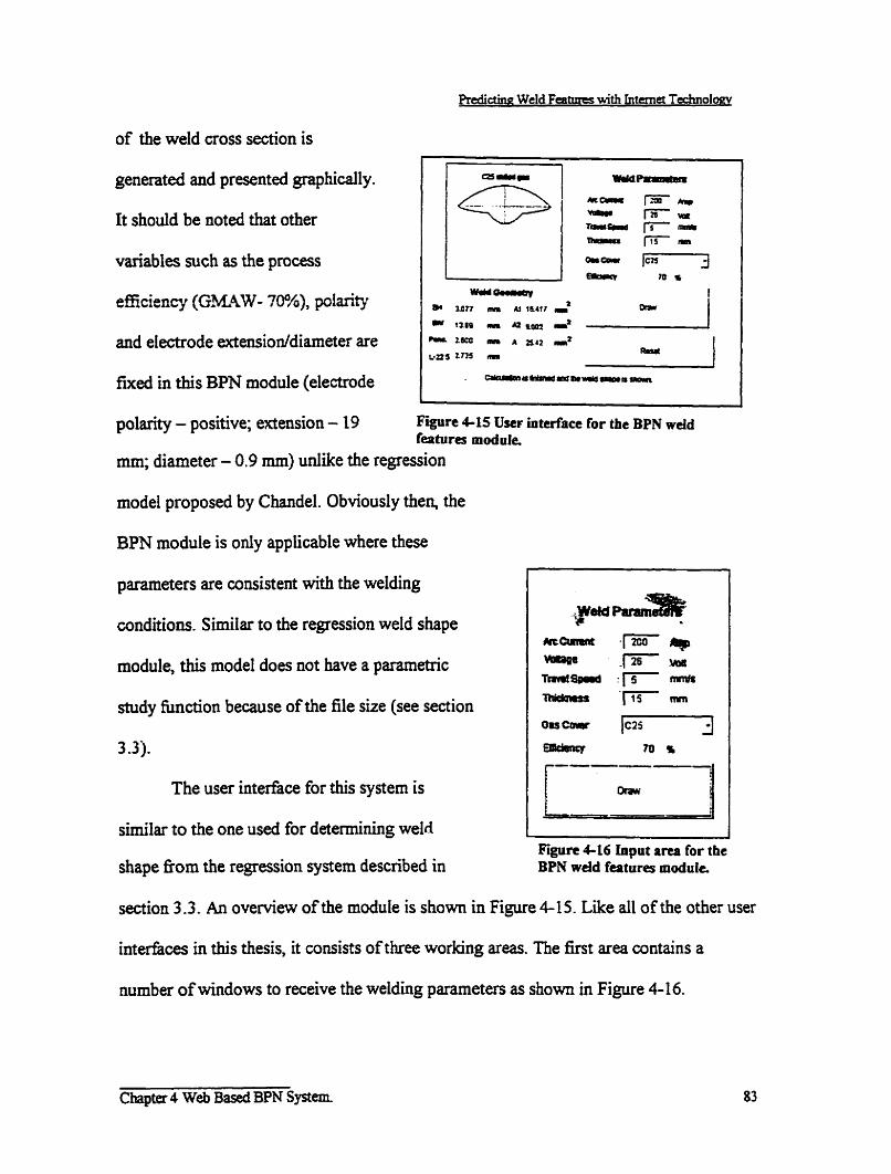
of the weld cross section is

generated and presented graphically.

It should be noted that other

variables such as the process

efficiency ( G M W - ?O%), pl*

and electrode extensioddiameter are

fixed in this BPN module (electmde

polanty - positive; extension - 19 Flgnre 4-15 User intvface for the BPN wdd fe~tures moduJe.

mm; diameter - 0.9 mm) d i k e the regrasion

model proposed by Chandel. Obviously then, the

BPN module is only applicable where these

parameters are consistent with the welding

conditions. Similar to the regression weld shape

module, this model does not have a pararnetric

study h c t i o n because of the file size (see section

3 -3 j.

The user interface for this system is

sirnilar to the one used for determinkg weld

shape f h m the regression system described in Figure 4-16 Input a m for the BPN wdd fatures rnoduie.

section 3 -3. An overview of the module is shown in Figure 4-15. Like al1 of the other user

interfàces in this thesis, it consias of three working areas. The first area contains a

nurnber of windows to receive the welding parameten as shown in Figure 4-16.

Figure 617 Rcsuit area for the BPN weld katurcs moduic

Predictinar Weld Features with Intemet Technoloqy 1

4

Figure 4-18 Plot aru for the BPN wdd ftatures modulc

The second work area receives the cdculated size and shape parameters as show

in Figure 4-17 and the third area is for a graphical display of the approximaze size and

shape of the weld, based on these parameters (Figure 4- 18). The shape is generated

acmrding to equations 2-48 to 2-58, following the system origidly pioposed by Chan

[4-11. in addition to the three work areas, there is a reset button and an error bar for

indicating the statu of the calculation

4.3.1 Verifkation of the BPN Weld Features Module

Like the cooling time and HAZ hardness evaluations, the data set selected for

evduating the web based weld size and shape algonthm is the same as that seleaed to

study the r e p s i o n counterpart, Le., the algorithm originally established by Chandel [4-

3,4]. The data base consists of weld cross sectional maurements taken from a large

number of GMAW beadsn-plate welds conducted a few years ago by Northem College

for the Carleton welding process research program [4-51. The data base consists of some

192 GMAW bead on plate welds ranging from 0.45 Id/mm to 1.43 kJ/mm with CC25 and

M2 gas cover. Al1 weld parameters were sectioned for the BPN mode1 training and cross

sectional measurements @ead width, bead height, penetration, deposit area and fiised


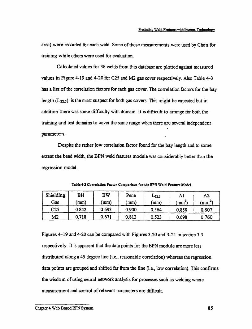
Weld Faîurcs with Intcrnct Tcchnoloey

are.) were recordeci for each weld. Some of these measurements were used by Chan for

training while others were used for evaluation.

Caiailated values for 36 welds fiom this database are plotted against measured

values in Figure 4-19 and 4-20 for C25 and M2 gas cover respectively. Aiso Table 4-3

has a list of the correlation ficton for each gas cover. The correlation factors for the bay

length fiz5) is the most suspect for both gas covers. This might be expected but in

addition there was some difficulty with domain. It is difiailt to arrange for both the

training and test domains to wver the sarne range when there are several independent

parameters.

Despite the rather low correlation factor found for the bay length and to some

extent the bead width, the BPN weld features module was considerably better than the

regression model.

Table 4-3 Cordation Factor Cornparison for the BPN Weld Feaairt Mode1

Figures 4-19 and 4-20 can be compared with Figures 3-20 and 3-21 in section 3.3

respectively. It is apparent that the data points for the BPN module are more less

distnbuted dong a 45 degree line (Le., reasonable correlation) whereas the regression

data points are grouped and shified fhr h m the line (i-e., low correlation). This confms

the wisdom of using neural network analysis for processes çuch as welding where

rneasurement and control of relevant parameters are difftailt.

Shielding Gas C25 M 2

chaPkr 4 Web Based BPN Synem

BH (mm) 0.842

0,718

B W (mm) O .693

0.67 1

Pene

(mm) 0.900

0,813

h.5

(mm) 0.564

0.523

AI

(mm2) 0.858

0.698

A2

(mm2) 0.807

0.760

I mtbnenbl Vdue (mm) I

I

1.5 r i

la 2 25 3 3 5

Exp.rbneritrl vdue (mm)

Figure 4-19 (c) BPN Deposaed Aha Comparisori

with C25 Cover Ga+

s ta 15 20 25 Experhierdtl Value (mm21

Figure 619 (c)

*v.irlrimii 3 5

Figure 4-19 (d) BPN Fusion h a Cosn9rifori

with C25 Cwer Gas

Fipm CUCompuisan of with measund wdd fentures (Northun College iwestr*gatioo - C Z gar cover): (a) bead heighZ (b) bead ddth , (c) penetration, (d) petration, (e) deposit area, (f) fusion a m

Chapter 4 Web baseci BPN System

r i r e 4-20 (e)

Pdictinn Weld Features Wnh Intenet Technolopy: BPN BW Cornpanson

8 10 12 14 16 18 20

m e (mm)

F i i r e 4-20 (b) BPN -5 Bay Lmgth Cornparison

Wrth M2 Cover Gas

FÏgtrre 4-20 (d) BPN Fusion h a Compvison

with M2 Covcr Gas

Figure 4-20 Cornparison of caiculated BPN wdd features with measured wdd features (Norihem Coiiege investigation - M î gas covu): (a) bead height, @) b u d width, (c) penetration, (ci) penetraîion, (e) deposit a m , (f) fusion area.

Chapter 4 Web B a d BPN Systern

4.4 Com~uter Reauirements for the Web Based BPN Svstem

The cornputer requirements for the BPN modules demibed in this section are

basically the same as those described in the section 3 for the regression modules since

both systerns have been coded using the Java prognim language. However, this is only

the case because there is no "training" for the BPN modules described in this section It

shauld be noted that as soon as there is training, the need for cpu resources increases

enormously. This is the situation for the web system described in chapter 5 where

training is assurned to take place in the web semer. This is disaisseci at length in that

section.

Predictinn Weld Feanires With Inremet Technotoay

Chapter Five

Web BPN Semer System for Modeling the Welding Process

fhis section dwribes the irnpiementation of the back propagation network (BPN)

weld process modeling system designed for the Internet The objective that is unique to

this work is to insist that BPN training take place on the server and thereby capture the

identity of the user, hisher raw experimental data and hisher eventual trained network

mode1 or models as the case may be. The raw data that is to be capturai consists of the

welding parameters such as voltage, cunenc welding speed, preheat temperature,

workpiece thickness, etc., and measured output quantities such as weld cooling times,

HAZ hardnesses and eventuaily weld sizes and shapes. The models that are to be

captured are trained neural networks that can r e m output calculated quantities such as

cooling times, HPIZ hardnesses, weld size and sbape, given arbitrary input welding

parameten voltage, current, welding speed, workpiece dimensions, etc. By capturing

these data centraily, a really large data base can be accurnulated fkom the contri butions of

many users which aui be used for the benefit of the entiie welding engineering

community.

The rnethodology used for this section has ken taken directly h m the

background material in section 2.4. The hardware and software used to generate the

system is descriid in section 5.1. The BPN weld process modeling system essentidly

consists of five software modules implemented on a semer which can be activated fiom a

-

Chapter 5 Web BPN Server Systern for Modeling the Weld Process 89

Predicting Weld Feahrre~ With Inteniet Technolow

user workstation These five modules are desigoated as follows: a raw data submission

module, a training module, a weight data submission module, a module for predicting

weld characteristics given the input welding parameters and a &ta view module. These

modules are descri i in section 5.2. The system was tested to evaluate its reliability by

comparing calculated values for bj with ithmeasured values. The cornparison is detaiied in

section 5.3.

5.1 Hardware and InstaIIed Amhcations Software

The first issue that &ad to be &ait with was that of a suitable semer. It seems that

the computational dernands of neuml network wodd be unreasonable for most

servers that are set up for more gened Intemet tm&c. Because of this, server

administraton (at Carleton and elsewhere) were reluctant to permit BPN training and

would not provide access. In the end it was decided that a server would eventually have

to be dedicated to the BPN weld pro- modeling problem But before committing to a

fully implemented on-line Internet server, local experirnentation to generate a workable

network and sort out a number of potentiaf problems was considerd necessary.

Therefore the system descri'bed in this chapter consists of two cornputers - one which

funaions as a server dedicated to weldhg process BPN modeling and the other a remote

PC workstation which functions as a user machine,

Chapter 5 Web BPN Setver S ystem for Modeling @e Weid Process

Predidna Weld Features With Imernet Technoloq

The wmputet environment for the development of on-line weld process neural

network modehg is show schematically in Figure 5-1. The two cornputen used in this

investigation will be referred to as the host

and client machines. They were Pertium PCs,

200 Mhertz machines. Each computer had

both a network card and was comected to the

other in a network contiguration While this

simple oetwork consists of only a host and

client for the purposes of developrnent, there

would be several client machines in a Mly

working on-line system in practice.

Communications and database applications

software were installed on the host computer

for recording information conceming the Figure 5-1 Host - dient computer confiuratioo

usen, raw experimentai weld procws data (welding parameters and measured weld

characteristics) and calculated (aained) BPN weights. In addition, computational

software for processing these data with BPN training was installed Once the BPN

network is trained for a given set of raw input da@ the BPN network weights are

recorded for fuhire reference, and it (the network) is ready to accept arbitrary welding

parameters and return calculated weld charactenistics to the user. With this configuration,

the only requirement of the client computer is a web browser to submit and access

infornation fiom the host computer.

- - --

C hapter 5 Web BPN Server S ystem for Modefing the WeId Process

Predictine Wefd Fegtures Wflh Imernet Technoloay

Linux was seIected as the host operating system primarily because it is designed

as network software, i.e., it is relatively easy to establish the host-client cornputer

relationship with Linux. In view of recent Linux developments in the commercial worid,

this wouid seem to have been a good choice. Moreover, Linux is considerably more

flexible for an application such as this, than altematives nich as Windows NT.

Following the installation of the operating system, a web server communications

software application cdled "Apache", was iastalled. Apache serves the host by receiving

information from a network client or nom the Intemet generally. The database

application MySQL was then installeci to pemiit recordhg the niw welding data, user

information and the nodal weights calculated fiom BPN training. It is couvenient to

think of the host machine as serving two environments, the web on the one hand and the

database on the other, These will be referred to as the web server and the riatahace Server

in the foiiowing discussion even though the hardware srver is one single hon machine.

FoIlowing the installation of the Apache communications software and the

MySQL database application software, the development environment was established by

instdling the computational software PHP - personai home page. Ln many ways PHP is

the server equivalent of the Java deveioprnent software except that it (PR) is designed

for host processing whereas Java is designed for remote deplopent The prirnary

b c t i o n of PHP is to carry out the network mathematical caiculations necessary for

m g . However, over and above this, PHP acts to interface the database server and the

web server. For example, a database request fiom an Internet user is facilitated by the

PHP software. The third fiinction of the PHP software is to create html pages for the

- --

Chapter 5 Web BPN Servet System for Modeling the WeId h c e s s

Preditina WeId Features With internet Technotoay

system. The software is quite flexible in this regard and the content of the html pages, so

generated, can be easily adapteci to the needs of the user or the requirements of the

system. For example, a raw data submission fonn can be easily changed to accommodate

the number of input/output data elements in any given data set and the number of data

records n d e d for training.

- -

Chapter 5 Web BPN S e m System for .Mode@ the WeId Ptocess

Predictinn Weld Featufes With Mernet TehnoIony

5.2 Svstem Im~lementation

In its sirnplest form the server systern for rnodeling the welding process consists of

the following five steps-for o d i n g - S O A w a r e modules: . . ..

raw data submission to the host cornputer,

training dam seleaion h m the submitted data or from &ta otherwise stored in the

host machine;

network training,

nodal weights stored in the host database;

trained module ready for use - output weld characteristics computed fkom arbitrary

input welding parameters (within the b i t s of the training).

Al1 modules are self contained, and the results of each can be stored in the host

database if necessary. Even though each module is independent, usen m u t go through ail

modules if they are to generate a useful working mode1 starting fiom raw experimental

data. In addition to the five modules identifiai above there is a sixth module incorporated

in the system - the "Data View Module". It is somewhat supplementary to the five

operational modules referred to above, but nonetheless very important The significance

of this module is detailed below. The foliowing describes each module in more detail.

In the interests of clarhy, the following data terminology (elernen~ record, set) are

hereby defined explicitly. An "elernenf' is the term used to refer to one quantity of the

data whether input or output, such as a voltage, a current, or a HAZ hardness. A "record"

refers to the input welding parameters that fix a welding situation and the correspondhg

output quantities (cwling time, HAZ hardness, weld size and shape). For the HAZ

Chapter 5 Web BPN Server System for Mddmg the Weld Process 94

Redictine Weld F e a ~ e s With internet Technolonv

hardness problem, a record would consist of the combination of relevant input welding

parameters - current, voltage, travel speed, plate thickness, and preheat, and the

corresponding output quantity, HA2 hardness. In this case there are six input elements

and one output elernent A &ta "set" refers to the entire collection o f records used for

generating a BPN module. One training data set contains several records and =ch record

contains several elements.

5.2.1 Raw Data Submission Module

The data submit module permits the submission

of both general information regardhg the data and user,

and detailrd idonnation, ie., the raw experimental data

weded for training. The infoxmation flow from the

client machine to the ho3 cornputer. The process

involved for this module is shown generally in the flow

diagram, Figure 5-2. The general Uiformation includes

the user's identity and email address, a password for

accessing the information, type of data (selected from a

predefined list), a short description of the data set, the

number of input/ourput elements, the total number of

input data records in the set, and submission method

The client interface screen form for the submission of

the general idormation is shown in the Figure 5-3.

When al1 of the gened information has been detailed on

Chapter 5 Web BPN S e m r System for Modehg the Weld RwrJs

Submission

Subrnission Cornpletion 1 """ fFciure 5 n 1

Figure 5-2 Flow diagram for the raw daîa submkion module.

Predictina Weld Features Wth internet Techno Ioa

screen, a confirmation screen is retunied (Figure 54). Following confirmation, the next

screen prompts for detailed welding parameter (voltage, currenf etc.) input and

corresponding output (cooling time, HAZ hardness, etc.) information (Figure 5-5).

- .

Badc to

BPN Training Data Set input ~ ~ m t Form ~ n f ~ ~

For Weld Application

Yom emaü addren: Ismorinis@chat. carlet.

Figure 5-3 Gaeral data submhioa form fbr the taw data submksioo modulc

The detailed information includes inpdoutput m e , and the numerical value of each

element For example, in the case of the cooling time problem, plate thickness, heat input

and preheat temperature are submitted as input elements while bs is the output element

Several cooling time records (inputloutput) are detailed on the screen which forms the raw

data set. When al1 of the records in the data base have been detailed on screen and

Chapter 5 Web BPN M e r Systern for Modding the Weld Process

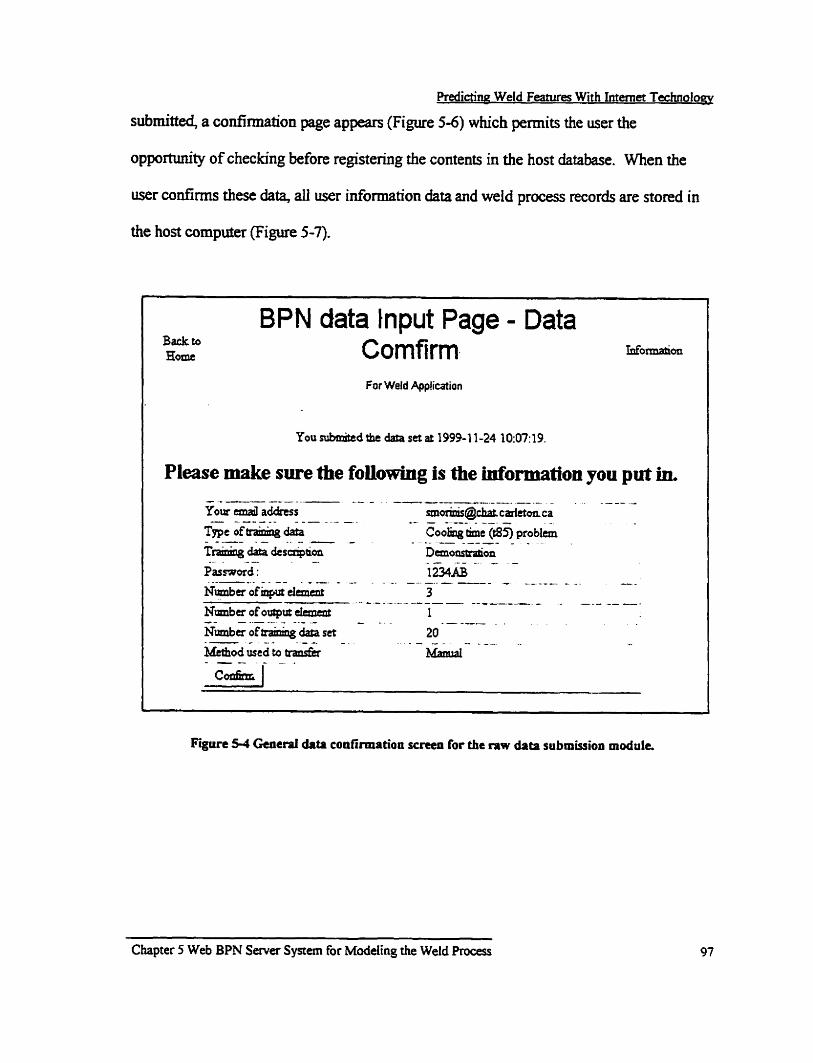
Predictina Weld Fearures With Interna Technoiogv

submitted, a confimation page appears (Figure 5-6) which permits the user the

oppomuiity of checking before r e g i s t e ~ g the contents in the host database. When the

user confirms these data, ali user information data and weld process records are stored in

the host cornputer (Figure 5-7).

BPN data Input Page - Data Cornfirm. For Weld App!icaion

YOU W d the dag set at 1999-1 1-24 10:07:19.

Please make sure the following is the iaformation you put in.

Figure 5-4 Generai data coafirmation s c n e n for the raw data submission module

Chapter 5 Web BPN Server System for Modehg the Weld Process

Predictinn Weld Features W a h Intemet Technology

Backb Home

BPN data Input Manually

This is the 3rd page of thP RPN dati input

- --* - -1 - -- _ I - - - - - - - - - 4 - - - .-

. . . - - - . - -- -r-- .Z. - --- ---- &&Lx 1 k t ) : . . ...---.-- .-.. _ . . . - .

Figure 5 5 Dulûed data subiaission form for the nw data SU bmkion modale.

Chapter 5 i'eb BPN Semer Srjtern For Modeling the Weld Process

Ba& to Home BPN data Input Page 4 (5 pages) ~ ~ 0 ~ 1

For Weld Applicaian I

Fwre 5-6 Detctiled data subrnUsion scmn for the mw data submbion moduk

Cbapter 5 We& BPN S a v a System for Modeling the Weld Process

Predictina Weld Features Wah berner Technolony

This is the last page of the BPN data input

Last step for data submision

Figure 5-7 Raw data subrnission complction scma.

5.2.2 Selectine Training Data

The bn ing &ta select module ailom usen to select training data from al 1 of the

raw data that raides in the host cornputer. A fIow

diagram for this module is shown in Figure 5-8.

For one reason or another a user may not have any

raw experimental data to work with or may not

choose to draw training data fiom that submitted to

the host In this case, the uscr cm initiate a search

ofthe host cornputer for data that is appropriate to

hisher situation by using keywords in the data

description or an email address that is associated

with a given set of data, or by simply listing al1

available mw data sets (Figure 5-9). In this Figure,

the keyword used for this presentation was cbdemo".

Data Conditions

Selectable R a w Dcrta Set

Figure 18 Flow diagram for the selaing training data modale.

- -

Chapto 5 Web BPN S a v a Symm for Modehg the Weld Rooen

Predictine Weld Features With latema Technoloav

When the search is complete, the list of the raw data sets will be displayed with

submission date, mail addresses of those who submitted &ta, type of data, description of

the data and the raw data ID index number (Figure 5-10). The data ID is an index number

for the data set, and clicking the link under the data ID number b ~ g s forward more

infoxmation regarcling the data set seledon ES show in Fiyre 5-1 1. The input'output

elements are identified, and the set records are listed together with check boxes. Those

records that are needed for training are checked and are then registered in the &tabase as

training data (Figure 5- 12).

f 1 B*. Home

BP N Training Data Selection

I For Weld &plicatian

Fïgure 5 9 D a i d data condition input suce. for the Kketing tnining data modulc

Back to Dataset Selection For Training Home L b d m


Subrnission Rate Earnil Addtess Type Of ~escriptioo ~ a t a ID Data

- - .--- - - ---- 19991 1-24 [email protected] ... Cooling rime 6ernonmation .. Data 1 O:O7:45

. * - - - - @35) problem set8 - - - -

Figare 5-10 List of mw data set for the rdecthg trrinhg data module

Cùapter 5 Web BPN Senta System for Moâeling the Weld Process 10 1

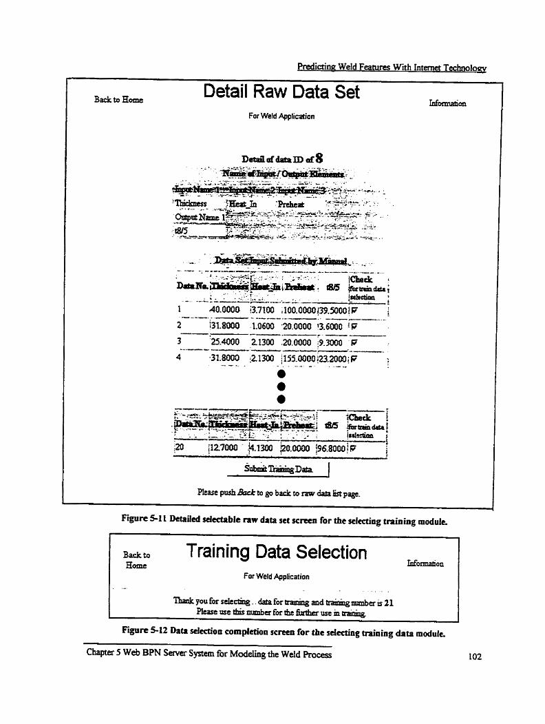
Redidnn Weld Features With btmnt Technoioey -

Backt0 Eomt Detail Raw Data Set M d a n


Training Data Selection For Weld Agplication

. - - , . -

Figure S I 2 Ihta sclcction completion SC- for the sdecthg ûainhg data module.

Chapter 5 Web BPN Savn System for ModdiDg the Weld Rocess

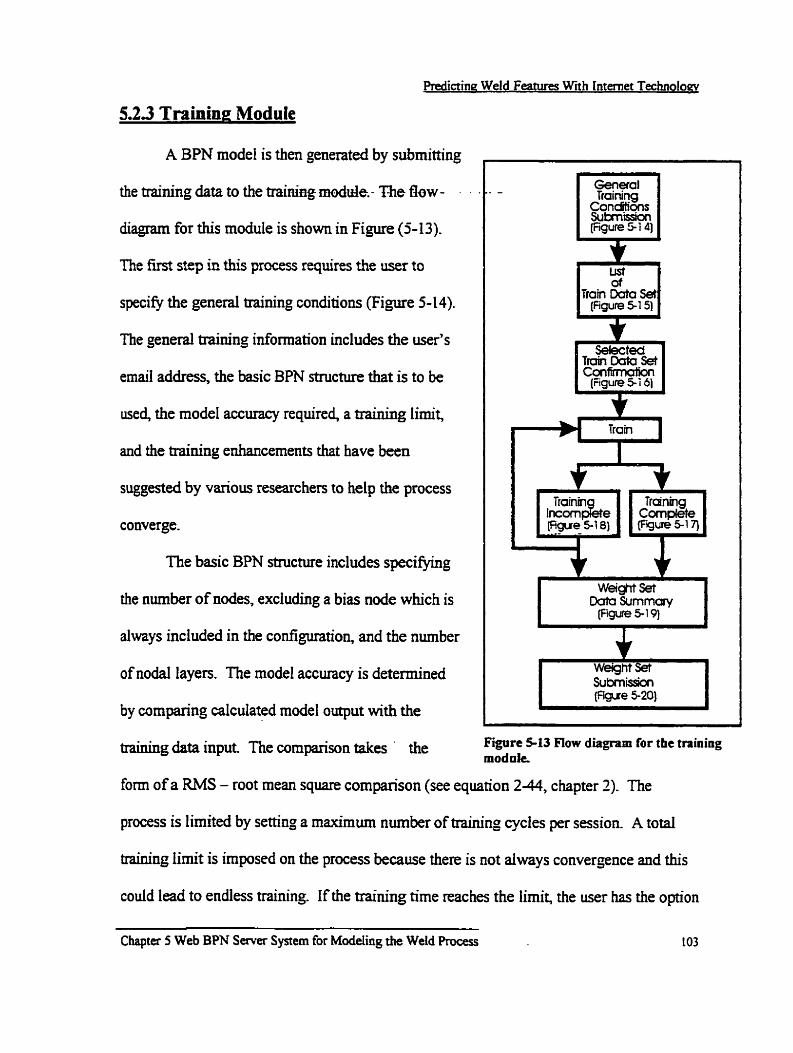
5.23 Training Module

A BPN mode1 is then generated by submitting

the training data to the training modide- The flow-

diagram for this module is shown in Figure (5- 13).

The tirsi step in this process requires the user to

s p i @ the general training conditions (Figure 5-14).

The general training information includes the user's

email address, the basic BPN structure that is to be

used, the mode1 accuracy required, a training Iimit,

and the training enhancements that have ken

suggested by various researc hem to help the process

converge.

The basic BPN structure includes specifjmg

the number of nodes, excluding a bias node which is

always included in the configuration, and the nurnber

of nodal layen. The mode1 accuracy is determineci

by cornpiring calculated mode1 output with the

Gepyal Training

Conditions S u b m i i (Figure 31 4)

Tram -ç'

training data input The cornparison takes ' the Figure 513 Fiow diagram for the training module

fom of a RMS - root mean square cornparison (see equation 2 4 , chapter 2). The

process is Iimited by setting a maximum number of training cycles per session. A total

training Iimit is imposed on the process because there is not always convergence and this

could lead to endless training. If the training time reaches the iimit, the user has the option

Chapter 5 Web BPN Server System for Modeling the Weld Process L03

Ptedictina Weld Features With Internet Techno1op;y

of restarîing or aborting the nin The available trainhg enhancernents are controlled by

the mornentum and through the use of Fahlman's derivative formulation These are

detailed in chapter 2, specifidly equations 2-42 and 245 respectively.

When d l of the information has ken provided to the module and the system is

prompteci to move fo~~ard, a list of the trahine data is retumed to the client cornputer

(Figure 5- 15). The list contains informafion about each data set, such as the submission

date, type of data, number of input/output elements, and number of records in the data set

A training data set is selected h m among tbose available and a confirmation of

submission appean as show in Figure 5-16. The screen also contains a summary of the

training session parameters - information regarding the BPN structure, detailed

information about the training dara set and the initial weights for training, which are

assigneci randomly between 0.5 and 4.5. When all of this information is confimed it is

submitted to the training module and training begins.

The training may be temiinated in one oftwo ways. If the RMS value specified in

the conditions for aaining is reached the training stops and a screen like that shown in

Figure 5- 1 7 appears. Basically, the screen contains the nodal weights determined from the

training On the other han& if the training does not reach RMS value within the specified

training period, the user is given the option of terminahg or restarting the training

(Figure 5-1 8). If the user elects to continue, the training resumes where it left off;

othenvise, the incomplete weight set is stored to the host cornputer if the user so decides

(Figure 5-1 9).

Chapter 5 Web BPN Semer Systern fat Modehg the Weld Process

Predictinn Weld Features With Intmet Technoloay

BPN Calc. Training Function For Weld Application

User Information Y o m d a d d r e s s : lsmorinis@chat. carleton. ca

BPN Calcnlntion Option

Figure 5-14 G e n d training condition submission form for the tirining module.

Chapter 5 Web BPN Server System for Modeiing the WeId Process

Predictina Weld Features With htemet Technolo~

Back to Home Available Training Data List

10 emes (out of 22 torail Number of Submission Tmie 'Type of Data

l n p ~ l 9 S A 1-25 Cooling tirne

- . Number of Nurnber of . Data

Dataset - =* - - - - - - - -- --- --

Data Set

l9%11-25 Cooling tirne 00: 24:56 (@S) ...

- . --- Data Set

21 r

I W S I 1-24 Cuoling tirne 21 :48:38 (tas) ...

- *

1993-1 7-21 Cooling tirne 08: 24: 23 (t8S) ...

- - - - - 'AI1 Records Nex 10 records

figure 515 List of train data set for the training modulc

Chapter 5 Web BPN Saver System for Modding the Weld Roass

Predictinp Weld Fea&ures With Intefnet Technoloay

Badcto BPN Train Condition Comfirmation Hame I n f ' a n

For Weld Applicttion

You rubmittd the data set ar 1999-1 1-25 lO:O9: 17.

---- - -- -- - - - - - - - - p i

N&a ofhidden 1 - - - - - - C - - - -- - -- - - - - - - .Nwher of nodes in fiddm hyer 5 - -- -- - - -- - -- - - - . N d e r ofinput cLmaa 3 t

.- - - - --- - - - - Nirmbu of output rlcmrnt 1 - - - - - - -- -- --- --- Nmba of minhg data sa 20 !

I n p r n ~ ~ ~ p h u * - - - t- -- - - - - - --- - - -- - - -ers Ha*-In - - - - - - - - - - - - - - - - Prchaat - - - a6 - -

3.710 l?E000- Sut 1 40.00û - - 39.500 Sat2 37.800 -

.. - - - - - - - 1.060 20.000 3.600 4 - - ---- - -

set 3 =y400 2 130 20.000 9.300 - - - - - - - - -.- - - - - - - - - * _ - Set4 31.800 2 130 155,000 23.200

--- -- - - - - ----- ~ e t - ~ 12700 - --- 2.1311 20.000 24.400 - - - - - - --- -- - - - - - _ --- Sat2û 12700 4.130 20.000 96.800

-.. - - .

Hidem Nodr 3 ---

0.010 -- -0,440

1

F i r e 5-16 Training condition summa y scmn for the training module.

Chapter 5 Web BPN Semer System for Modding the Wdd Rocas

Pdict inp Weld Fea~rres Wth htemet Technology

r d

BPN Training data Page I ~ * ~ ~ ~ For Weld Application MOrmatirn 1

RMS mur L 0.30022 +the CO- O ~ O

d Figure 5-17 Training completion screen for the m i a g module

I

BPN Training data Page I H- f p f d o n

I For Wefd Agplication I

Training maynot done due to counter and îhe rms vaiuc is 0.29208 and thc R-EbS Pahtt k 0.04 wim coliater of 6

The dcuk ion has not beutrrtched the speci6ed RMS due . DO yoa~~ a n r to contmue ûaining?

4 figure 5 1 8 Training incomplete screen for the tmhing modulc

Chapta 5 Web BPN S a v a Sy~em for Modeling the Weld Pm-.

Predidnn Weld Features Wfih interna Technoloq

Ba.cktoHornt BPN Training Result InfbimatiO1l


Fire 519 Wcîght set summary screen for the training modult

4

Chapta 5 Web BPN Serva System for Moddiiig the Weld Pmcess

Redictinn Weld Features With hernet TechnoIoav

I Back t~ E ~ c BPN Training - LAST PAGE- ~ ~ r m a t i ~

for Weld Application

Th;rnlrc for training the data set.

I Ba& !O PFPT =tu2

Figure 5.20 Weight set submhioii cornpletc scrcen for the tror-ning module

5.2.4 Weight Data Submission Module

This is the module designed for submitting

the weight data set submission to database in the host

cornputer. The process involved for this module is

shown in a flow diagram (Figure 5-21). The process

here is similar to that used to subrnit raw data to the

database. The infornation is of two types, general

ulfomation and detailed weight data. The fim

interface requires the input of the general infomiation

(Figure 5-22). The general information includes the

user's identiv and email address, a short description

of the data set the number of input/output nodes

(elements) and the submission method When the

general information is sent to the daîabase a screen

0 Figure 521 Fiow diagnm for the weight submission module.

aises calling for the detailed information (Figure 5-24) after the general information is

confinned (Figure 5-23). The detailed information inciudes input'o utput name, eac h

inputloutput range and the numerical weight data For example, in the case of the mling

Chapter 5 Web BPN Server System for Modehg the Weld Proass . 110

tune problem, plate thickness, heat input to the process, and preheat temperature are

submitted as input names, while &ps is used for the output name together with the

conespondhg training ranges. The user then submits weight numbers h m the training

(previous modde) as shown in the Figure. When these data are documented on the

screen, a confirmation page is displayed (Figure 5-25) for checkhg purposes &fore

registering the contents to the database. Ifthe user c o d ï m s the content al1 the records are

stored in the host computer data base (Figure 5-26).

Chapter 5 Web BPN Smer Synmi for M o d e h g the Weld Pmceu

Predictinp Weld Featwes Wnh intemet Technology

Back to

BPN Trained Weight Data Hom Set Input Form M-OLI


N d a r af'nodes h the second h Ü b n 1 -Pteasc se&&-

Figure 5-22 GtDerPl information submission f om for the weight data submission module.

Chapter 5 Web BPN Server Synem for Modering the Weid R o ~ s

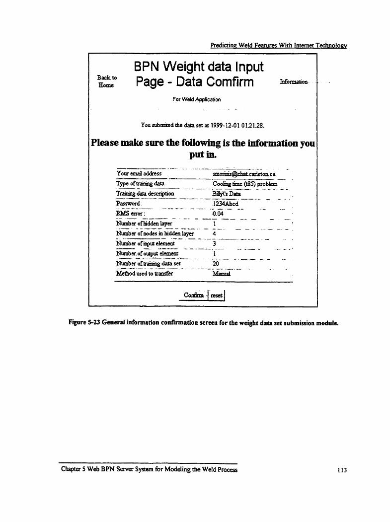
Predictih~ Weld Featum Wi t h Imemer Technoiooy

Back to

BPN Weight data Input Home Page - Data Comfirm I P f o ~ ~


You submiotd thc data set at 1999-12-01 01:21:28.

PIease make sure the foUowing is the information you put in.

Figore S23 Gea~ml bformation confirmation semen for the weight data set submksioa module

Chapte 5 Web BPN Server System for Modding the Weld Pmcen

Predictinn Weld Features Wfih Mernet TechnoIosy

Back to Home

BPN Weight Data input faformation


You NbmiÉ tht data set at l999-l2-O 1 01:2I:58.

Epre 5-24 Detailai hformntion submission form for the wu'ght subminion moduk

Chapter 5 Web BPN SaverSyncm for Moddlig the Weld Process

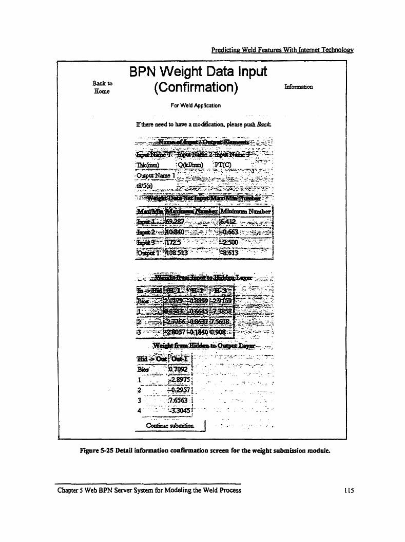
Predictina Weid Featums WÏth Intemet Technolopv


- . . . - - - - - -

Ifthm w d to hm a mo&&on, plcase push k k

Fiire 5-25 Detail i n f o ~ t i o n confirmation screen for the weight submission module

Chapter 5 Web BPN Server System for Modding the Weid Prwss

Predicrinor Weld Features With lnternet Technoiopy

Back to Last step for BPN weight

~ ~ m c data subrnision ~ormarioa

Far WIld Application l 'Lhank you for the wei& chta submission Pieaseckk~togobackto&cmainmrrnri

Fipn S26 W+ht data suhmk<im cnmplete .wma for the weight chta -set suhmioion m d u l r

5.2.5 BPN Caledation Module

When the training is complete the nodal

weights can be used to generate a weld process

model, custom generated to match the choice of

the training data As mentioned several times in

this thesis, custorn training is important because

it implicitiy takes into account variables that

anse nom operator skill and elsewhere that

cannot othewise be quantified. I f the mode1 is

generated with training data from the wr's job

shop or rnanufâctunng operation, then the model

implicitiy incorporates operator tradition and

other effects unique to that operation. This is not

possible d e n universal models (regression,

physical rnodeling) that have been generated

ekewhere are us&

List

Weig ht Data (Figure 5-28)

Input Data

Submission [Figure 5-29]

Calculation Result

(Figure 5-30]

Figure 5-27 Flow d i m Cor the BPN dcuiation module

C hapter 5 Weô BPN Saver Systern for Modeiing the Wetd Rocess

Predictina Weld Feahires With Zntemet Technolonv

The BPN cdculation module is essentiaily the weld process mode1 arising from the

training. Users can subrnit arbitrary welding &.suneten (within the limits of the training)

and calculateci output quantities are returned. The flow diagram for this module is show

in Figure 5-27. The first step in this process is selecting a set of weights. A list of

available BPN models (Le. list of weight sets) in the host cornputer is displayd oii the

screen as shown in Figure 5-28. Listeù in the display are bahhg subrnission date, email

address of the trainer, the type of trainhg data, data description, and aaining ID (an index

nuinber for each set of weights). From this information usen can decide which set of

weights are consistent with their needs. In many w e s the user wïll also have been the

''trainer" in which case he/she will use die set of weights that was detennined during the

training session. However in other cases, potentiai users may not have training data and in

that case they c m still select fiom among those models (training weights) that are

contained in the data base.

A weight set is selected by c l i chg the training ID index number on the screen,

which among other things, b ~ g s forward a screen that lists the limits of each of the input

data elements (Figure 5-29). For example, if the training covers the welduig current range

150-300 amps, then calcuiations are oniy valid within this current range. When the

welding parameters have been submitted, the calculate button is activateci and output

quantities (cooling time, HAZ hardness, etc.) are displayed on the screen (Figure 5-30).

Chapter 5 Web BPN Semer Systern for Modeling the Weld Process

Predictina Weld Features Wah Intemet Technoloav

Back to

Weight Database lnside List Home For Calculation rdbmati~

Far Weld Application

- - -- 10 entries (ouf of 322 total) - .--- - --- - - - -- - . - - TIme mf Description Train ID Subrnission Eamil Addnss

- 1 99S1 1-25 - Cooling ,Trained-on-line. Wet ohr Set

. - 00: 14: 15 - - 322

1 99Ç.11-20 am@ mer Trained-onJine. VVeioht Sei 1 6: 20%

- - - .- 321

1 99S11-20 shun@ Orner ~rained-on-line: VVeioht Set 04:44: 1 3 - -- - -- al 1999.11-20 shun@ m e r test on ~ov26- Weioht Set 04:34:44 -- - * - - - 319

1 9 9 W 1-1 9 HAZ@NOV18 Hardness ~rained-on-fine. Weiaht Set l6:OO:28

f -- - - - - -- ---y

318

Figure 5-2û List o f weight dita set for the BPN alcuhtioo module.

Back to Komt

Detait Weight Data Set For Wald &plication

PLarepushWtogobackro~data6rrpagt .

Fiire S29 Input data submkion fonn for the BPN dcdat ion module.

Ehapter 5 Web BPN Semr System for Modding the WeId Roctss

Predictina Weld Features With Intemet Technology

Back to Home

Detait Weight Data Set For WeM Application

Phse push Back to go back to raw data k page - -

Figure 5-30 C.aicuiation muit for the BPN dculation modulc

5.2.6 Data View Module

The &ta view module dlows users to see both raw experimental data and the

weight data sets in the host cornputer. It is necessary to view the data in this way when

trying to decide the applicability of one or another mode1 in practice. Therefore, this is a

very usefui module in the system. The flow diagmm for this module is shown in Figure 5-

3 1. A search facility is available in the module that will list the data sets requested as

show in Figure 5-32. The search retums a list containing the data submission date, the

email address of the trainer, the type of data, a description of the data and a data ID index

nurnber. Wiîh that information a user can display the raw input experimental data or

weight data set by activating the data ID index number as shown in Figure 5-33.

Chapter 5 Web BPN Server Systern fOC Modding the Weld Process

Prcdictmg Weld Fesbaes With Intanet Technolw

These data can also be displayed in "text

format", as shown in Figure 5-34. By saving the

information to a client local hard drive, the file can

be used with the NNWorks software.

It may be recalled that the NNWorks

software is the PC stand alone version of the BPN

wntained in this thesis. It was authored by Dr. B.

Chan (5-1). The downloaded raw data can be used

to train NNWorks for one application or another

while the weight data can be used to generate a

Mly working NNWorks mode1 directly. This is a

ûesired Data

Condifions [Figure 532)

(figure 5-33] IMI Detailed

[Figure 5-34]

very important contribution it essentidy is Figure $31 Fiow diagram of the data view moduie

another way of using the Internet to assist the welding community in exchanging useful research

data and weld process modeling information It has been fouad that training on an Intemet

server is iimited. The diniculty is that the PHP generated software for BPN training wnmmes

considerable cornputhg resources and may occupy a server for long periods of time which is

not very good in a practical sense. By downioading the raw data and using NNworks the

training is carried out locally with efficient software and then there is little problem with

cornputhg resources; yet useful data has been exchanged and the user enjoys vimially dl the

benefits of the server training system. Moreover, if the server is occupied with training, it is not

accessible to other users and this wiil lead to fnstration and problems in practice. This or

Chap ter 5 Web BPN %mer Systan fa MaMing the Weld Fhxes 120

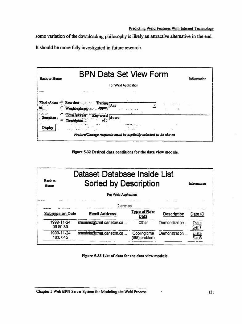
Redictine Weld Features Wnh intanet Technolooy

some variation of the downloading philosophy is likeiy an amactive alternative in the end.

It should be more fully investigated in future research

Back to Home BPN Data Set View Form

For Weld App!icatian . -- .- a

F î r e 5-32 D a M data conditions for the data view module

Dataset Database lnside List Sorted by Description

-- - - ---- . . . 2 -

2 emies ----- - - -.--- - - * - - - - ---

Subrnission Date Eamil Address Of R a ~ Description Data ID - --- -

Data - -- - -- 19991 1-24 srnorinis@chatcar(eton.ca ... Orner Demonstration ... C m 09: 50: 35 .-. 7 -- --- - -

- -- 1993-1 1-24 [email protected] ... Cooiing time Dernonsta~on ... ~-315

1 0:07:45 - - (t85) problem 3: 8 - -- -- - -- - - --

Fgure 5-33 List of data for the data view modale.

Chapter 5 Web BPN S a v a System for Modehg the Weld Process

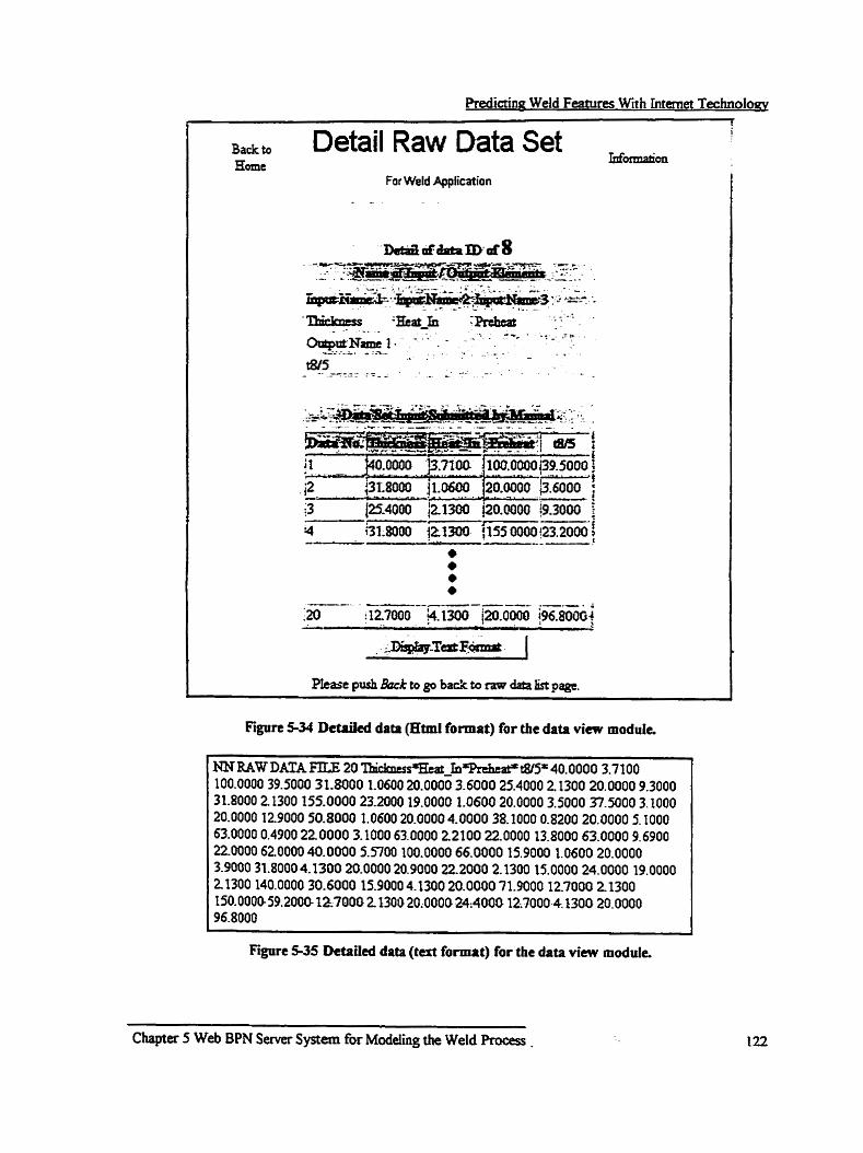
Predictino WeId Features With Intemet Technolopv !

Detail Raw Data Set ! Bade to Eamt WOzmation

For Weld Aqplication

PkastpushBmcktop backtornadatalllpagc.

Figttre 1 3 4 DcWed data (Html format) for the data v i m module.

& I Figure 5-35 Detniled data (tat format) for the data vkw module.

C w e r 5 Web BPN S e m r System for Modeling the WeId Proan -

Predictina Weld Faturcs Wth Intemet Technoloay

5 3 BPN Training Module Ve,rïfi~ation

Verification of the Internet weld process modeling system included both teting

the performance of the BPN training module and measuring the accuracy of the output

quantities dculated w*th a trained model. Performance was tested because there were

difficdties with the trairiirig process. It seans that serm ûaiaining is time consuming,

much more so tban stand alone PC training. There may be many reasons for this, the

efficiency of the PHP application software compared with Ci+, the complexity of the

semr systern, etc. The exclusive-or @OR) problem is one that is widely used to test

neural network systems and therefore it was incorporated in this study to examine

performance. Since the cwling t h e and the KAZ hardness problems were used by Chan

to test his system when he generated W o r k s , the stand alone version of the server

system descn i in this thesis, they aiso formed part of the test study. The complexity of

the test networks rangeci fiom simple (an exclusive-or, XOR, problem), to medium (the

cooling tune problem) to cornplex (the HAZ hardness problern).

For d l perfomance tests, the network initiai weights were set randornly benveen

+0.5 and 4.5 [5-21, and al1 input and output parameters were normalized between 0.95

and 0.05 (see chapter 2 4 1 - 1 ). The Ieaming process was not limiteci in this case but

continued until the RMS fimit was reached When the training was completed, the

number of leaming cycles otherwise calied epochs was recordeci Four separate leaming

trials were camed out for each probfem, except for the HAZ hardness problern where the

training time became measonably long. In that case the term "urueasonably long tirne"

became the result of the test,

Chapter 5 Web BPN Semer System for Modeiing the We td Process <

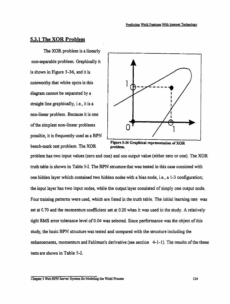
PrcdiPrcdictirig: Weld Features With internet Technology

5.3.1 The XOR Problem

The XOR problem is a linearfy

non-separable problem Graphically it

is shown in Figure 5-36, and it i s

noteworthy that white spots in this

diagram cannot be sepanited by a

straight line graphically, Le., it is a

non-linear problem. Because it is one

of the simplest non-linear problems

possible, it is âequently used as a BPN

bench-mark test problem. The XOR Figrrre 5-36 Graphieal representation o f XOR pro blem.

. . -

problem has two input values (zero and one) and one output value (either zero or one). The XOR

tmth table is shown in Table 5-1. The BPN stmcture that was tested in this case consisted with

one hidden layer which contained two hidden nodes with a bias node, Le., a 1-3 configuration;

the input layer has two input nodes, while the output layer cunsiaed of simply one output node.

Four training patterns were used, which are listed in the truth table. The initial learning rate was

set at 0.70 and the momenturn coefficient set at 0.20 when it was used in the study. A relatively

tight RMS ermr tolerance level of 0.04 was selected. Since performance was the object of this

study, the basic BPN structure was tested and compared with the structure including the

enhancernents, momenturn and Fahlman's denvative (see section 4- 1 - 1). The results of the these

tests are shown in Table 5-2.

Chaptcr 5 Web BPN Saver System for Modehg the Weld Rocess

Predictinu Weld F e u e s With Intemet Technolqy

Table 5-1 XOR Tmth Table

Table S 2 Pedormanct o f Differeat Learning Enbancement Algantbm for the XOR Problem

Input 1 O 1 O

1 Basic Momentum 1 Momentum with 1 1 1 (NO enhancement) 1 (a= 0.20) 1 Fahlman7s derivative 1

Input 2 O O 1

Output O I 1

As the table shows both enhancements improve the performance of the learning

O 1

Trid 1 Trid 2 Triai 3 Trail4

t Average

process, especially the combination o f the Faidman's derivative and momentum. In this

1

case the average leaming time was decreased some 30%. This is strong evidence that the

(epoch) (min) 1633 (4)

extra wmplexity of including both momentun and Fahiman's derivative is certainiy

5.3.2 The Cooüng Time Problem

(epoch) (min) 2097 ( 5 )

The cooling t h e problem is considered to be more cornplex than the XOR

(epo~h) (min) 1266 (3)

problem because it includes some noisy data (scatter in the resuits) and there are more

2306 (6) 1 1471 (3)

data records per set avaifable for training The experiment reported in this work

1325 (3) 1361 (3) 1705 (4) 1414 (3)

243 1 (6) 2 173 (5) 2136 (5)

paralleleci the work of Chan's [5- 11 who useci three input etements (heat inpu& plate

I

1934 (4) 1894 (4) 1849 (4)

thickness, and arnbient temperature) and one output element ( W 5 cooling time) with one

hidden layer which had 5 nodes including a bias node. Chan used this arrangement to

Chapter 5 Web BPN Server Systern for Modeling the Weld Process

pndicting Weld Feahaes Wi?h Intanet Technology

test the performance of the stand alone PC BPN system incorporated in NNWorks and it

seemed like a good idea to use the same configuration for cornparison purposes. Twenty data

records [ 5 4 , 5,6,7] were used in the training which are listed in the Appendix 1. The results are

tabulated in Table 5-3. The results dernonstrate conclusively that the combination of the two

enhancements is most &&ive in reducining the training tirne. Once again, using the enharicement

combination provided the best overail epoch reduction

As expected, the training thne is considerably longer for the cooling time problem than it

is for the XOR problem (compare Table 5-2 with 5-3). It seems reasonable to suppose that this is

because there is more data for training in the cooling time problem and then again the added

complexity uiat there is with this problem also likely contributes to the increase in training time.

In effect, training the cooling time network takes about twice as long as the XOR probiem

Moreover, the training for this problem with the Intemet semer system took about 20 times as

long as the same test with NNWorks as documenteci by Chan [5-11. There may be many reasons

for this but it is Orely due to merences in Server generated PHP software rather than the more

efficient C* software used by Chan.

Table 5-3 Performance of Differcnt Ira- Enhanament AlgorittÜriJ for the Cooüng T i e Problern

Basic (No enhancements)

Chapter 5 Web BPN Sem6system for McdeliBg îhe Weld Raas

Triai 1 TriaI 2 Trial 3 Tnal4

Average

Morne- (a = 0.20)

Momentum with Fahlman's Denvative

(epoch number) (min) 4090 (57) 5626(78) 405 1 (5 6) 3999(56) 444 1(62)

(epoch number) (min) 2966(4 1) 2360(33) 378 l(52) 3038(42) 3036(42)

(epoch nun: 206 1 1768 1526 1914 1817

Table 5-4 Madel Accurrcy Resuit For The Cao@ Tirne Probiem

However, the correlation factor and the standard deviation of the difference between

m e a ~ u ~ e d and calnilateci values would indicate that it û a fairly acairate system -

CorreIat ion Factor Average Diff Standard Deviaticin

certainly this kind of accuracy would be welcomed by the welding cummunity.

5.3.3 The H A 2 Hardness Probiem

The H A 2 hardaess problem selected for testing was taken directly from the study

of Yurioka [5-31, which consias of four inputs elements (coolhg time, two carbon

equivalents, and a carbon content) and one output element (HA2 hardness). ?hirty data

records were used to train this model, the details of which are documented in Appendix

II. Because the problem is much more cornplex than the XOR and cooling time

problems, the BPN structure consisted of 8 nodes in a single hidden layer, four nodes for

the input and a single output node. The combination of Fahiman's derivative and

momentum enhancements were used for this experiment.

The calculation tune for the hardness problem was much longer than that for the

cooling time problem. Though both enhancements were incorporated the time to

convergence was considered unreasonably long (greater than one day) and the test was

Trial 1 0.96 4.73 3.70

aborted It is not reasonable to tie up a server with training for days at a time. Moreover,

training times this Iong can lead to numerical difficulties such as round-off errors and

basic reliability can becorne a problem The time consuming dificulty is likely software

Chapter 5 Web BPN Semer Systan for Modehg the weld Process

Trial 4 0.97 4.70

Trial 2 ( Tria1 3

3.37 1 3.37 1 3.46

0.97 4.55

0.97 4.57

Predictina Weld Features Wrth Internet Tectuiology

efficiency as mentioned above with regard to the cooling t h e problem. This is certaidy

an issue for future re~eafch and development before the system can be deployed.

While BPN server weld process rnodeling has k e n demonstrated and al1 the

necessary elements are in place, there is considerably more work to be done.

Nonetheless, the principk of semer training and mode1 deplojlment, together *ith

accumulating user identities and raw data has been established. It is for future thesis

tesearchers to sort out some of the difficulties that have been identified in this thesis and

to bring the system into practice.

Chapter 5 Web BPN Semer System for Modeiing the Wetd Process

Predictine Weld Fearures With Intemet Technoloqy

Chapter S '

General Discussion

The general objective of this thesis was to bring the weld process modeii.ng

software, that was initially generated by Chan [6-11, to the Intemet for the benefit of the

welding engineering community at large. While the Chan software is in the marketplace

under the name of Weldsofi (regession based software) and NNworks (neural network

based software), it is not used to the extent that might be expectd, and yet it bas b e n

said that this software is very useful for practicing engineers in the welding and

fabrication industries. The basic premise of this thesis is that Intemet availability would

address this problem. In this regard, Intemet Java applet versions of both Weldsoft and

NNworks have been presented in this thesis which in efEect addresses the objective

dircdy.

in addition to the Java applets, a server based BPN weld process modeling facility

has bem demonstrated which adds an imporiant dimension to the issue of availability. In

this system, Intemet users submit raw experirnental data to a dedicated weld process

server, whereupon BPN training takes place. At the same tirne the raw experimental

training data and information conceming the user is captured by the server and made

available to the welding engineering community as a whoIe. Moreover, the trained

mode1 is captured by the server and dso made available to usen at large. The potential

of this system for capturing and assembling a reaily large database is considered to be an

important contribution for the benefit of entire welding community-

Chapter 6 General Discussion -

Predictma Weld Feahats With Intanet Technology

Java applets perform well especially the applet for cornputing cooling time (800

to 500 OC) and fiom this the applet for calailating H A 2 hardness. The software applets

reside in a central Intemet server and are downioaded to.a user on demand. A

convenient user intefice form has been incorporateci in the HAZ hardness mode1

containhg windows for aü input quantities. Welding parameters (voltage, aurent,

welding speed, arc efficiency and workpiece thickness), and the workpiece chemical

composition are input through the interface form Calailated HAZ hardnesses are

retrrmed. Parametric study is possible whereby HAZ hardness as a finction of any of

the welding parameters or workpiece chemical composition variables can be displayed

in graphical form. The reliability of the software has ben confirmed by comparïng

calculated HAZ hardnesses with m e a d values. There is little else to add but to

declare that the objective, insofar as calculating cooling times and HAZ hardnesses is

concerned, has been met.

lava applets have also been presented for cornputing weld size and shape,

similar to the software containeci in Weldsoft and NNworks. By and large, the Java

applets are similar to the Weldsoft and NNWorks software. Both technologies

incorporate convenient user interfaces and both have been verified against experimental

measurernents. However, the applet software does not yet permit parametric study

whereas the stand alone PC software does have a parametric study fàcility. The primary

reason for this is that, among other things, there is not enough room on one interface to

resenre space for pafametric graphical display in this module. This researcher opted for

the simplicity of a single interface where the calcufated results and a display of the weld

Chapter 6 Genaal Diçcussion 130

Predicting Weld Feahlres With Intemet Technolony

cross section can be presented on one screen One or two m e r screens would be

necessary for parametric display and for a display presenting the effect of polarity and

gas cover which is contained in the stand done version There is a lot to be said for the

simplicity of the one screen display presented in this thesis. Nonetheless, a suggestion

for M e r work would be that the parametric snidy and plarity/_eas cover screens could

and probably should be added at sorne time in the fûture.

It shouid be noted that the Java applet systems may be considered "univenal" in

the sense that the algorithms are meant to be applied to a wide range of welding processes

and welding configurations. This is useful because it preserves the simplicity of

traditional mearch where modeling is always intended to be universal as long as the

assumptions and conditions under which the mode1 was generated are consistent with the

application The diffculty with the welding process in this regard is that it is not in

general a fuily controlled process where the set conditions define the resdt. The culture

of the welding community is such ?hat operator skill and tradition are involveci in the

process and these c m o t be quantified In this sense the so-called universai rnodels are

lirnited and practitioners must know that the results of such caiculations are at best

approximations. Perhaps the best feaîure of such models is the possibility of parametnc

study where engineen can study the effect of one or another variable on the expected

output.

However, n e d network technology offers the researchers and engineen tools

that are able to address the problem of ski11 and culture based parameters, at least in part.

As long as welding professionals are consistent, neural network software " l e m s what to

Chapter 6 G d Discussion 13 I

expect &orn them in terms ofoutput and computations can implicitly take skiil and tradition into

account, In particular BPN welding models can be custorn generated for a job shop or even for a

single welding operator. This was Chan's intent when he introduced the software NNworks to the

weldiag community a few years ago. While NNworks has certainly had an impact on the welding

community, the objective ofthis thesis is to make it available on the Intemet and to insid that

training take place on the server. By insisting on central processing, trained models can be stored

and made available to the welding community as a whole; but even more than that the raw

experimentai data used for aaining cm be captured almg with the identity of those who elect to

use the process. A large database of training data would be a vaiuable resource for the welding

community as a whole. Data q d t y and reliability would certainly be an issue with such a

system. However, presumably users wodd select only those data for which they had confidence.

However, generating an on-he BPN system for modeling the welding process has not been

easy. In fact it has meant a great deal of work. One of the Erst obstacles faced by the author was

arranging for server s e ~ c e s . In the begiming it was assumed that either a university server or an

industrial server could be found where administraton would be willing to house the weld modeling

sohare. However, it was found that most serven do not have the cumputational or database

development applications. Beyond this most administrators were concemed that the computing

resources necessary to run the weld modeling system would be excessive and in addition,

maimainkg such a system would be dificuit. In view of these dÎfEculties, it was conciuded that a

dedicated aistom configureci server wouid have to be used for this program. Therefore, it became

necessary to learn server technology and not only conventional server technology but advanced

Chapter6 ccnrcaiDiscussion 132

Predictinn Weld Features With Intemet Technoloay

server computational fùnctionaiity as well. While server technology is interesting this

was not part of the initial objective.

Nonetheless, this researcher persevered, assembled a local network consisting of a

m e r and a client machine. A server operating systenq ccmmunications software,

computational software and database software were instailed and a BPN weld modeling

system generated. Interface software was arranged for the convenience of users. In fact

this system is faithful to the original objective in ail respects. Usen submit their raw

experimental data (cooling times, HAZ hardnesses, etc.; and welding parameters) to the

system which are stored in the database together with information on the user. Training

data is selected (on-line) fiom a rernote client machine and submitted to the training

server software. Training is done within the server and a set of training weights rehrnred

to the user and to the database for central storage. The system is then ready to accept

arbitrary welding conditions (within the limits of the training) and return calailateci

outputs (HM hardnesses, etc.). In effect this accornplishes the objective of making the

BPN system available to Intemet users in the welding commUNty and at the same time a

registry of users, experimental data and aistom designed models is stored in the database

for general use. Moreover, the on-line system eliminates a lot of upgrading problems

because the software is stored in the host cornputer and a one time upgrade in the server

automaticdl y upgrades ail the soflware for users.

Whife the objective has been demoastrated, there are difficulties that will have to

be addressed before the system is ready to be fully implemented on-line. The fkst is the

length of tirne necessary for training. As documented in section five, several hours are

C hapter 6 G e n d Discussion 133

Predictina Weld F e a m Wfih Internet Techoloqy

necessary in some cases to baiSn a single model. While training is going on, the server is

Iargely dedicated to this activity. During this t h e the server is either not functiond for

other users and at best,it meam a very slow response for other hctions such as

communicating with the database. This will not be workable in practicey as Intemet usen

are accustomeci to instant response of some b d . It wodd seem that a dramatic increase

in server cornputhg resources or a ciramatic increase in the efficiency of the training

software would be needed to solve this problem It may be that a dedicated

computational cornputer could be arranged in parailel with the server, whereby training

jobs would be spooled for processing and the weights retumed sequentially to the

database. C l d y more work is needed to address this problem.

Altematively, this researcher has suggested that the ûaining data could be

downloaded to client machines for off-line training with NNworks. in fact the "Data

Viewn module is designeci for that purpose. The dificulty with this is that there is no

guarantee tbat the user wodd resubrnit M e r trallied module to the server, nor is there

any guarantee that the user wouid Ieave hidher niw tmining data It would essentially be

an hoaor system. On the other hand, it would give use^^ access to dl of the data and

models that have be registered in the database. It seem to this author that this kind of

"data exchange" philosophy offen considerable potential and it shouid be considered

carefully in the future.

Another difficulty with the current demonstration systern is file tramfer. For the

convenience of users, automatic file transfer technology between modules should be

irnplemented As it now stands raw data and weight set submission are transfemed

Predictirip Weld Features With internez Technolocq

manually between modules, and there is aiways the possibility of transfer error, quite

apart from the inconvenience. Yet this is not as easy as one mi@ suppose. It is not

possible to send data in normal text format, since it has to be registered in the database

software. To do this, special fomiattng is required. Data -fer from one format to

another is tmublesome at the moment but is something that should be addresseci in future

work

While there are difficulties with the demonstration system that have to be

addressed before it becornes a fully implemented Internet system, this author would

contend that the principle of on-line, caphlnng user iiormation and

experimental data has been established Captrned data is then availabie to any w r in

keeping with Intemet tradition Thus the objective of making the weld process modeling

software widely available to the weiding engineering commuuity has been met

Chapter 6 General Discussion

c m

Chapter Seven

Conclusions and Cunfnbutions

1 ) Java venions- of the PC standabne weld process software "WeWft" and +

'Wnworks" for computing HAZ hardnecses md w l d fêatwes (weld sk and shpe)

have been presented. The software is housed on a centrai Intemet server and

downloaded in response to client request for off-line remote processing.

2) To evaluate the Java software computed values of HAZ hamesses and weld ske and

shape have k e n compared with experimentally measured values and geaeral

agreement was found

3) A server system that accepts raw irairing data fiom clients and r e m trained cusiorn

generated weld proçess models to the user has been presented At the same time user

information, raw training data and trained models are captirred by the server database

for general use by the welding c ~ m m ~ t y .

4) The training process causes host cornputer overioad, which would not be acceptable

for such a system in practice. Further work will be necessary to address this probiem.

5 ) There is a need for automated data exchange between modules in the server system

which will also have to be addressed before this system becomes practical.

Chaptet 7 Conclusions and Comributions

Predictiw Weld Features with Internet Techoloqy

Chapter Eighf

Future Work The shortcomings of both the applet remote processing system and the on-line server

system have been discussed at length in the thesis, especially in the general discussion

Therefore they will only be listed here as a summary:

1. A parametric study faciiity should be added to the weid featllfes Java applet In al1

likelihood this would involve arranping for two additional user screens, one for

graphical presentation and one to present pictorial weld cross -on representations

depicting the effect of poiarity and gas cover.

2. The difficulty of excessive training time for the on-line BPN weld process system

m u t be addresseci This might involve mon efficient software, or it might involve a

cornputer paraileled with the server and dedicated to training only. A spooling

system would have to be arrangeci for processing training jobs sequentiaily and

weights would then be remed to the database for recording.

3. The data exchange principle put forward by the author whereby, training data is

pmided fiom the server to the client for training off-line with NNworks rnight be

developed to address the training time problem. in this way remote client machines

could be used to provide the cornputing resources necessary for training. The server

wodd then be free for communication with clients.

Chapter 8 Future Work

Weki Featurcs with Intemet TcchnoIoq

4. Automatic &ta exchange between modules should be developed to avoid the inconvenience

and potential for emr caused when cornputeci results are transfened manually.

5. The weld features BPN system should be extended by training and testing with data for

welding processes other than GMAW, e-g., SMAW, SAW, FCAW, etc.

While many other suggestions couid be put foxward the five suggested here would

undoubtedly move the technology a long way toward a fully working system. !t is the authors

view that these are the issues that shotdd receive priority and focus.

Chapter 8 Future wo*

Refemces References for Chapter 1

1-1) Shiegiey J. E., Mtchel L. O., Mechanical Engineering Design, 4%dition, McGraw-HilI Book Company 1983, p 175.

1-2) Bibby, MJ., Yurioka, N., Ghetto, J. and Chan, B., "Predctive Methodr for Mmtogng HMugen in Welding Applicatiolls". White paper prepared for the International Workshop on "Managing Hydrogen in Welding Applications, h w a , October 6-8, 1998, Proceedings, pp 1 - 15.

1-3) Yurioka N., Impact of Weld'mg Research on Steel Composition Development, Materiais and Design, Vol. VI, No.4 1985, 19pgs.

1-4) Suzuki H, Carbon Equivalent and Maximum Hardness, Transaction of Japanese Welding Society, 1984, Vol. 15, No. 1, p 25

1-5) Satoh K., Terasaki T., Estimation of H A . Hardness, Jap. Weld. Society. General Meeting, 1979, Vo1.25, p 98.

1-6) Terasaki T., Study ofpredictive Equations of Thermal Factor and Hardness Related with Weld Cold Cracking, Iron and Steel Japan, 1981, Vol. 19, p 145.

1-7) Yurioka N., Ohisita S., Tanehiro H., Shidy on Carbon Equivalent to Assess Cold Cracking Tendency and Hardness in Steel Welding, Proc. Conference On Pipeline Welding in the 80's. March 1981.

1-8) Yurioka N., Okumura M., Kasuya T., Prediction of HAZ Hardness of Transformable Steels, Metai Construction, Apd, 1987, p 217R

1-9) Chan B., Software For Welding Engiaeen, Masters Thesis, Department of Mechanical and ~ e r o s ~ a c e Engineering, Carleton University., 1990.

1-10) Chan B., Predicting Weld FeaGires Using Artificiai Neural Network Technology, Doctoral Thesis, Department of Mechanical and Aerospace Engineering, Carleton University., 1996, p57.

1-1 1) Chan, B., Bibby, MX, and Holtz, N., Redîcting HAZ Hardness with Artifcial Neural Networks, Canadian MetailurgicaI Quarterly, Vol 3 4 No. 4, 1996, pp3 53-3 56.

References for Chapter 2

2-1) Easterling K, Introduction To The Physical Metallurgy Of Welding, 2* editioq Butterworth- Heinemann 1992, p 2.

2-2) Easterling K, Introduction To The Physical MetalIurgy Of Welding, 2d edition, Butterworth- Heinemann 1.992, p 126.

139

Easterling K., Introduction To The Physical Metallurgy Of Weldiag, 2& edition, Butt erworth-Heinemann 1992, p2.5.

Adams. C. M. Jr., Cooling Rates and Peak Temperatures In Fusion Welding., Welding Research Supplement, May 1958, p210s

Yurioka N., Impact of Welding Research on Steel Composition Development, Materials and Design, Vol. VL, No.4, 1985,19pgs.

Chandel R S., Mathematical Modeling of GMAW Feahires, Modeling and Control of Casting and Welding Process IV, 1988, p109.

Chandel R S., An Investigation into the Electrode and Plate Melting Efficiencies of SAW and GMAW Processes, Report MTL 89-10(J), Metals Technology Laboratories, CANMET/EMR, Governrnent of Canada, Ottawa, Ontario, KIA OG1, 1989.

Rosenuial D., Mathematical Theory of Heat D i s t r i i o n During Welding and Cutîing, AWS Welding Journal, Vo1.21 NOS, May 1941, p220s.

Rosenthal D., The Theory of Moving Sources of Heat and Its Application. to Metal Treatments, Transaction of ASME, Vol.43, No. 1 1, 1 946, p849.

2- 1 0) Jhaveri P., Moffit W. 6. Adams C. M Jr., The Effect of Plate Thickness and Radiation on Heat Flow in Welding and Cuttîng, Welding Journal, Vol. 41, No. 1, 1962, pl2.

2-1 1) Yurioka N., Impact of Welding Research on Steel Composition Development, Materials and Design, Vol. VI, N0.4, 1985,19pgs.

2-12) Suzuki K, Carbon Equivalent and Maximum Hardness, Transactions of the Iapanese Welding Society, 1984, Vo1.15, No. 1, p z .

2-1 3) Satoh .K., Terasaki T., Estimation of HAZ Hardness, Jap. Weld. Society. General Meeting, 1979, Vo1.25, p98.

2-14) Terasaki T., Study of Predictive Equations of Thermal Factor and Hardness Related with Weld Cold Cracking, Iron and Steel Japan, 198 1 Vol. 19, p 145.

2- 1 5) Yurioka N., Ohisita S., Tanehiro H-, Shidy on Carbon Equivalent to Assess Cold Cracking Tendency and Hardness in Steel Welding, Proc. Conf On Pipeline Welding in the 80's, March 1981.

Yurioka N., Okumura M., Kaniya T., Prediction of HAZ Hardness of Transfonnable Steei, Metal Construction, Apnl, 1987, p 2 17R.

Chan B ., S o k e For Welding Engineers, Master Thesis, Department of Mechanical and Aerospace Enginee~g, Carleton U., 1990, pp 12-5 1.

Rumelhart D. F., &ton G., Williams R J., Leaming Interna1 Representation by Error Propagation, in Parailel Distributed Processing, Vol. 1, edited by Rumelhart and MeClelland, Cambridge Mq the ha Press, 1986, pp 3 18-3 62.

Dixon R, Neural Nets: Building on Nature's Design, Course Notes, Carleton Professional Development Center, Ottawa, A p d 1993.

Ebehart R C., Dobbins R W., (editors), Neural Network PC Tools: A Practical Guide, Academic Press, Inc., San Diego, CA, 1990, pp 40-43, pp 240-242.

Fahlman S. F., Faster L e d g Variations on Backpropagation: An Empirical Study, in Proceedings of 1988 Connectionist Models Sumer Schooi, D.S. Touretzky, O. Hùlton, T. Sejnowski, (editors), Morgan, Kauhan, 1988.

Chan B ., Predicting Weld Features Using Artificial Neural Network Technology, Doctoral Thesis, Department of Mechanical and Aerospace engineering, Carleton U., 1996, pp 57-86.

ho Y., Bessyo, K., Weldability Formula of High Strength Steels related to Heat- AEected-Zone Cracking, 1 1 W Doc., IX-57668, 1968, pp 145, Transaction of Japanese Welding Society, 1968, Vo1.37, No.9, pp 983-991, 1 1 W Doe. M-63 1 - 69, 1969, Iâpgs.

Sudci , It, Carbon Equivalent for Steel Weldability, 11 W Doe., IX-1230-82, 1982, Dpgs.

Bhadeshia K, Materials Algorithms Project, httdlwww mmi - ac ui~mad.

William Oates (editor), Welding Handbook, Vol. 2, Welding Processes, edition, American Welding Society, 1996.

Reference for Chapter 3

3- 1) Rosenthal D., Mathematical Theory of Heat Distribution During Welding and Cutting, AWS Welding Jorn& V01.21 NOS, May 1941, pp22Os-234s

3-2) Rosenthal D., The Theory of Moving Sources of Heat and Its Application to Metal Treatments Transaction of ASME, Vo1.43, No. 1 1, 1946, pp 849-869.

Jhaveri P., Moffit W. G. Adams C. M. Jr., The Effécî of Plate Thickness and Radiation on Heat Flow in Welding and Cutting, WeIding Journal, Vol. 4 1, No. 1, 1962, pp12.

Adams. C. M. Jr., Cooling Rates and Peak Temperatures In Fusion Welding., Welding Research Supplement, May 1958, pp2 10s - 215s.

Kohno R, Jones S. B., An Initial Snidy of Arc Energy and thermal Cycles in the Submerged Arc Welding of Steel. the Welding Institute; IIW ûoc., 8 111 978/PE, Dec. 1978. Yurioka N., Oshita S., Tamehiro H., Study on Carbon Equivalent to Assess Cold Cracking Tendency and Hardness in Steel Welduig,, Proc. C o d On Pileline Welding in the 803, 198 1, 15pgs., JWS WM-784480, 1 1 pgs, 1980.

Signes E. G., A Simplified Method of Calculating Cooling Rates in Mild and Low Alloy Steel Weld Metals, Welding J o d , Vol. 5 1, OctOber 1972, pp475s.

Yurioka N., Ohisita S., Tanehiro H, Study on Carbon Equivaient to Assess Cold Crachg Tendancy and Hardness in Steel Welding, Roc. Cod. ûn Pipeline Welding in the 807s, March 1981.

Yurioka N., Okumura M, Kaçuya Tw Prediction of HAZ Hardness of Transformable Steel, M e t . Construction, Apd, 1987, pp 217R

Satoh K, Terasaki T., Estimation of HAZ Hardness, Jap. Weld Society. Generai Meeting, 1979, Vol. 25, pp 98.

Terasaki T., Study of Predictive Equations of Thermal Factor and Hardness Relateci with Weld Cold Cracking, Iron and Steel, Japan, 1981 Vol. 19, pp 145.

S u d K, Carbon Equivalent and Maximum Hardness, Transaction of Japanese Welding Society, 1984, Vol. 1 5, No. 1, pp 25-33

Bala S. R, Pond S., Weldablility and Fomablility of Two Candidate Stels for Offshore Structure and Arctic Vessels, AMCA Intemationai Ltd, Repon No. 1 - 1834141F, December 1983, Part B: Table2, Table B2.1.

Chan B., Software For Welding Engineers, Master Thesis, Deparunent of Mechanicd and Aeros~ace Engineerine, Carleton U.. 1990- DD 12-5 1-

Chan B., Chandel R, Bibby M-, A Software System for Cornputhg the Size and Shape of GMA (Gas Metal Arc) Welds, ASME J o d of Engineering for industry, presented at ASME, Production Engineering Division, 199 1 Winter Annual Meeting, Atlanta Hilton and Towers, Deccember 1-6, 199 1, ' Welding and Ioining Processes', ASME PED Vol. 5 1, Welding and Joining Rocesses, 199 1, pp 2 15-225.

Chan B., Bibby M. Yang L. J.. Chandel R7 A Discussion of Algorithms of Predicting Submerged Arc Weld Shapes with Workpiece Edge Reparatioa, Manufacturing Science and Engineering, PED-vo. 64, presnted at the 1 1 4 ~ a n n d ASME AM^ Winter Meeting in New Chieans, Nov. 29 - Dec. 3, 1993.

Chan B., Bibby M., Chandel R, A Software System for Anticipating the Size and Shape ofsubrnerged Arc Welds, Journal of Material Processing Technology, Vol 40., No. 3 4 , pp 249-262, Jan. 1994 (also presented at the Asia Pacific Conference on Material Processing, Singapore, March, 1993). Chan B., Predicting Weld Feahires Using Artificial Neural Network Technology, P h D. Thesis, Department of Mechanical and Aeroçpace engineering, Carleton U., 1996.

Beaudoin M, Expanding the Cariaon University Weldsoft Package, Graduate Technicd Report, Welding Engineering Technology Department, Northern Collage at Kîrkland Lake, April, 1993.


Chan B., Predicting Weld Features Using Artificid Ne& Network Technology, Ph D. Thesis, Department of Mechanical and Aerospace engineering, Carleton U., 1996.

Bala S. R, Pond S., Weldablility and Formablility of Two Candidate Steels for Offshore Structure and Arctic Vessels, AMCA International Ltd, Report No. 1 - 183414/F, December 1983, Part B: Tablez, Table B2.1.

Chandel R S., Mathematicai Modeling of GMAW Features, Modeling and Contml of Casting and Welding Process N, 1988, pp 109- 120.

Chandel R S., An Investigation into the Electrode and Plate Melting Efficiencies of SAW and GMAW Processes, Report Mn. 89- 10(5), Metals Technology Laboratories, CANMETEMR, Govemment of Canada, Ottawq Ontario, K1A OGl, 1989.

4-5) Beaudoin M-, Expanding the Carieton University Weldsoft Package, Graduate Technical Repo* Welding Engineering Technology Department, Northem C d k g ~ & K & & Lake,-A& -1-993: - - - -


Chan B., Predicting Weld Features Using Artificid Neural Network Technology, Ph D. Thesis, Department of Mechanical and Aerospace engineering, Carleton U., 1996.

Dixon R, Neural Nets: Building on Nature's Design, Course Notes, Carleton Professional Development Center, Oûawa, Apd 1993.

Yurioka N., Oshita S., Tamehiro K, Shidy on Carbon Equivdent to Assess Cold Cracking Tendency and Hardness in Steel Welding,, Roc. C o d On Pileline WeIding in the ~ O ' S , 198 1, lspgs., J W S WM-784-480,lI pgs, 1980.

Rcxiruges P.E.L.B., R-ogenon J. K, How Weld Metd Thermal Cycles Detemine the Toughness of SAWs, Welding and Metal Fabrication, April 1980, pp 183- 192.

Van Adrichem Th. J., Kas J., Caiculation, Measurement and Simulation of Weld Thermal Cycles, Smit-Weld N. V. Nijmegen., Holectecniek, Netherlands, June 1971, Vol. 1, NO. 1, pp 2-1 1.

Bibby M. J., St Louis M., TrauttmansdorfYF., Goldak J. A, Predicring the Fusion and HAZ Efardness of WeIds, A Report to AMCA Corporation, Carleton University, Febniary 18,1983.

Bala S. R, Pond S., Weldabitity and Fomuibility of Two Canadiate Steels for Offshore Smcture and Arctic Vessels, AMCA International Ltd, Report No. 1 - 1 8 0 14E, December 1983, Part B: Table3, Table B2.1.


6-1) Chan B., Predicting Weld Features Using Artificid Neural Network Technology, P h D. Thesis, Department of Mechanical and Aerospace engineering, Carleton U., 1996.

Cooling Time Data

This appendix is composed of three different groups of cooling time data. They

were all used for verieng the cooling tirne s o h e u d ~ d b e d in chapten 3 md 4 The

fist set is extracted form the work of Kohno et [3-51 which is based on the submerged

welding process. The second set is gas metai arc weld cooling times from the work of

Signes et al [3-71. The Iast set of cooling time is based on the shielded metal arc weld

investigation of Yurioka et al [3-81.

Mict inn Weld Fe9turés With Interner Technoloqy

Yurioka et al [3-81 SMAW bs experimentd data (qF= 0.80 for calculating heat input).

flow ( m d s ) (mm) ( k h r n ) 3-D 24 1 120 3.58 ( 20 0.64 20 1 3.01

Predictinn Weld Features With Internet Technolw

Signes et ai [3-7] entire GMAW bs experirnental data ( T ] ~ = 0.7 for caiculating heat input).

Heat 1 Voltage 1 Curent 1 Speed 1 Thickness [ Heat in 1 Preheat 1 &/s

25.5 2.20 21.1 9.80 25.5 3.30 204 64.20 25.5 1.65 204 15-90 25.5 2-75 149 28.70 25.5 3.30 93.3 3 1 -50 25.5 2.20 93.3 13.80 25.5 3.30 21.1 20.60 19.1 3.30 93.3 77.90 19.1 2.20 93.3 23.80 19.1 1-65 ai. i 7-95 12.7 1-10 149 23.40 25.5 2.20 304 28.20 25.5 2.20 204 32.10 25.5 2.20 149 18.70 25.5 2.20 93.3 15-20 19.1 1.65 204 33.30

Appendix I CooIing Time Data 148

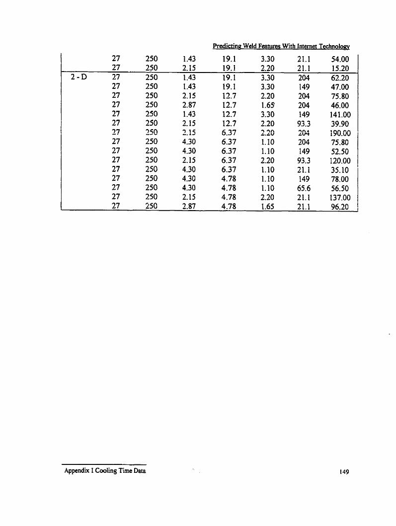
Prodictine Weld Femms With Internet Technolm

Appendk 1 Cooling rune Data

AMCA Hardness Data

AMCA [3-131 HAZ hardness data were used for venfying the network hardness

laiowledge as outlined in Cbapter 3 and 4. The onginai study includes both 800 to 500

O C cooling t h e and HA2 hardness. The coolkg time data are included in Appendix IV

as the work of Bala et al 13- 131.

A MCA Experimental HAZ Hardness Data /3-131.

AMCA SAW t8,s experimental data are listed in Appendix IV.

AMCA 13- 131 tested steels chernical composition. - --

Steel C Mn Si Cr Mo V Ni Cu P S Nb AI N CE Pcm BI 0.05 0.42 0.23 033 0.21 0.002 1.03 1.06 0.01 0.009 0.042 0.023 0.010 0.448 0.200

AMCA HAZ Hardness (VI-IN) [3- 131.

r

hls (s) 3.1 5.0 6 4 10,O 13,8 2 1.5 31 ,O 48.5 62.0

Steet BI 308 277 27 1 267 254 246 246 250 250

I

Steel 82 - 379

350 306 283 281 -.

265 238 246 -- 238

Steel B3 433 340 348 308 290 277 246 238 227 --

Appendix III

Gas MdaZ Arc Weld Size Data

Note from thesis supervisor W. Bibby: The data that was to occupy pages 153-164

were to corne from the weld size and shape investigation h m Northern College [ 5 4 ] -

182 sets of GMAW data with C25 and M2 cover gas. These data were used as the

training and verifmition information for the weId size and shape features module. Mr.

Morinishi did not finish this section but the data may be found in the doctoral thesis of

Dr. Billy Chan [SI].

NOTE TO USERS

Page(s) not included in the original manuscript are unavailable from the author or university. The

manuscript was microfilmed as received.

This reproduction is the best copy available.

UMI

SA W Experimental Cooling Time

The following are the submergeci arc weld 800 to 5 0 0 ~ ~ woling times - data

gathered from four individual works: Rodniges et al [54], Adrichem et ai [5-51, Bibby et

al [Ml, and Bala et al [5-71. These &ta were used for training and verifjring the cooling

time networks as outlined in Chapter 5.

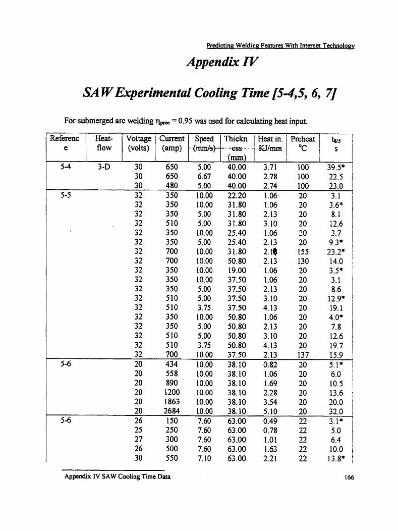
Predictina Weldinn Features With Internet Technolony

For submerged arc welding q, = 0.95 was used for calculating heat input

Appendix IV SAW Cmling Time Data 1 66

Referenc ' Heat- ' Voltage

5-4 3-D 30 650 5.00 40.00 3-71 100 39.5" 30 650 6.67 40.00 2-78 100 22.5

Curent (amp) (volts) e

Speed - (mmk)--- fiow

bs s

Thiclai -ess- - (mm)

Heatin Qfm

heheat O C

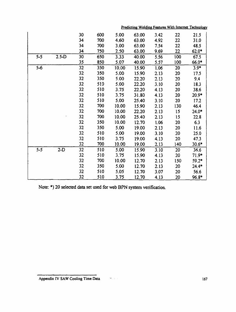
Preditina Weldina Features With Intemet Technoloay

Note: *) 20 selected data set used for web BPN system veification

Experimental H M Hardness Data

The following are the original HAZ hardness data £?om the work of Yurioka et ai

[3-6]. These data were used to train and test the backpropagetion networks for estimating

HAZ hardness, given the 800 to 500 OC cooling time and steel chemical composition as

describecl in chapters 3 and 4. Hardnesses, cooling times and the chemical compositions

of the fourteen steels used in the investigation are included in this Appendk

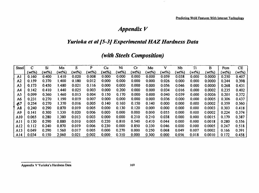
Predictinu Weld Features Internet Technol~gy

Steel

Yurioka et al /5-31 Experimental HAZ Harthess Data

(with Steels C'position)

Appendix V Yuriaka's Hardness Daia

Pcm CE (w%) (wt%) 0.250 0.407 0.244 0,398 0.268 0.431 0.235 0,402 0.201 0.372 0.306 0,437 0.359 0.560 0,303 0.418 0.224 0.374 O. 179 0,387 0,280 0.556 0.247 0.518 O, 166 0,391 0.172 0.458

Predictina Weld Features W i ~ h Internet Techn~logy

Notes : *) The 30 sets of training data,

Appendix V Yurioka's Hsrdness Data

€¦ · a cornputer system for predicting heat-affected zone (haz) hardness and weld €eaues...

Documents