a coupled in-situ measurement of temperature and kinematic

HAL Id: hal-01737079https://hal-mines-albi.archives-ouvertes.fr/hal-01737079

Submitted on 18 Apr 2018

HAL is a multi-disciplinary open accessarchive for the deposit and dissemination of sci-entific research documents, whether they are pub-lished or not. The documents may come fromteaching and research institutions in France orabroad, or from public or private research centers.

L’archive ouverte pluridisciplinaire HAL, estdestinée au dépôt et à la diffusion de documentsscientifiques de niveau recherche, publiés ou non,émanant des établissements d’enseignement et derecherche français ou étrangers, des laboratoirespublics ou privés.

A coupled in-situ measurement of temperature andkinematic fields in Ti-6Al-4V serrated chip formation at

micro-scaleMahmoud Harzallah, Thomas Pottier, Rémi Gilblas, Yann Landon, Michel

Mousseigne, Johanna Senatore

To cite this version:Mahmoud Harzallah, Thomas Pottier, Rémi Gilblas, Yann Landon, Michel Mousseigne, et al.. Acoupled in-situ measurement of temperature and kinematic fields in Ti-6Al-4V serrated chip for-mation at micro-scale. International Journal of Machine Tools and Manufacture, Elsevier, 2018,10.1016/j.ijmachtools.2018.03.003. hal-01737079

https://hal-mines-albi.archives-ouvertes.fr/hal-01737079

https://hal.archives-ouvertes.fr

A coupled in-situ measurement of temperature andkinematic fields in Ti-6Al-4V serrated chip

formation at micro-scale

M. Harzallaha, T. Pottiera∗, R. Gilblasa, Y. Landonb, M. Mousseigneb, J. Senatoreb

a Institut Clement Ader (ICA), Universite de Toulouse, CNRS, Mines Albi, UPS, INSA, ISAE-SUPAERO, Campus Jarlard, 81013 Albi CT Cedex 09, France

b Institut Clement Ader (ICA), Universite de Toulouse, CNRS, Mines Albi, UPS, INSA, ISAE-SUPAERO, 3 rue Caroline Aigle, 31400 Toulouse, France

Keywords

Primary shear zoneDigital image correlationInfrared Thermographymicro scaleFast imaging

Abstract

The present paper describes and uses a novel bi-spectral imaging apparatus ded-icated to the simultaneaous measurement of kinematic and thermal fields in or-thogonal cutting experiment. Based on wavelength splitting, this device is usedto image small scale phenomenon (about 500×500µm area) involved in the gener-ation of serrated chips from Ti-6Al-4V titanium alloy. Small to moderate cuttingspeeds are investigated at 6000 images per second for visible spectrum and 600images per second for infrared measuresments. It allows to obtain unblurred im-ages. A specific attention is paid to calibration issue including optical distortioncorrection, thermal calibration and data mapping. A complex post-processingprocedure based on DIC and direct solution of the heat diffusion equation is de-tailed in order to obtain strain, strain-rate, temperature and dissipation fieldsfrom raw data in a finite strains framework. Finally a discussion is addressedand closely analyzes the obtained results in order to improve the understandingof the segment generation problem from a kinemtatic standpoint but also for thefirst time from an energetic standpoint.

Introduction

The constant interest in understanding and mastering the ma-chining processes has led researchers to focus more and moreclosely on the cutting phenomeon. In recent years, variousmodelling attemps has met with the need of reliable mea-surements to either discriminate and/or validate models [37].The use of post-mortem analysis such as chip morphologyand SEM analysis [57, 67, 17, 61, 60] remains the most com-mon approach. Force components measurement in real timetrough Kistler dynamometer is also very popular and has be-come almost dogmatic in machining research [53, 33]. Tem-perature measurement using thermo-couples inserted either inthe part or in the tool insert has also been investegated to reg-ister macro scale heat generation [24]. The use of such globalquantities (chip morphology, cutting force and tool tempera-ture) has proven worthy but limits the understanding of localphenomena such as strain distribution and temperature gen-eration.

To overcome this very issue, some studies have been ded-icated to the assessement of in-situ measurement of thermo-mechanical quantities. The use of Quick Stop Devices hasbeen widely developped in the machining field with some in-tresting results [12, 34, 30]. More recently, full-field measure-ment techniques have been successfully implemented for ma-chining purpose. They offer a real-time and in-situ insight ofthe thermomechanical fields through surface measurements.Such data exhibit of course a different nature from those

within the bulk of the material but remain valuable eitherfor phenomena understanding or for model validation. Per-forming full-field measurements of any nature in cutting con-ditions exhibits two major difficulies i) the size of the observedarea and ii) the rapidity with which the phenomenon occurs.These papers can be sorted in two main categories: strainsmeasurements and infrared (IR) temperature measurements.

Though strain measurements at micro-scale are well doc-umented in a SEM environnement [27, 21, 52], the speedrequirement in cutting condition has prevented researchersto adopt this approach to obtain experimental data. Fewstudies have focused on such measurement, in quasi-staticor dynamic conditions, through optical microscopy [29, 42].Indeed, optical microscopy can easily be coupled with highspeed imaging and thus offer a way to work around thetwo difficulties mentioned in the above. The use of Digi-tal Image Correlation (DIC) has enabled the computation ofstrains and strain rates at microscale and low cutting speed(Vc = 6.10−4m.min−1) along continuous chips in [13] and athigher speed (Vc = 6 m.min−1) in serrated chips in [15, 44].Nevertheless, this technique requires unblurred images andis thus often used at low-to-moderate cutting speed. Athigher cutting speed, Particle Image Velocimetry (PIV) is of-ten preferred eventhough it cannot be used for serrated chips[19, 23, 22]. One noticeable exception is the work of Hijaziand Madhavan [28] which have developed a complex dedi-cated device composed of four non-intensified digital camerasset in dual frame mode to perform a 4 unblurred images ac-

∗Tel. +33 (0)5 63 49 30 48e-mail: [email protected]

Harzallah et al. – 2018 2

quisition at 1 MHz and thus use DIC to retreive strains. Morerecently, the improvement of high-speed camera spatial res-olution enable Baizeau et al. [6] to perform DIC at highercutting speed (Vc = 90 m.min−1) , this work is not directlyfocused on the chip formation but rather on residual stressesin the generated surface and is thus performed at a lowermagnification.

Temperature measurement at tool tip within the infraredwaveband have been investigated in the early 2000’s by var-ious works includig the pioneer work of [47] which uses IRpyrometry. However, thermographical studies are very sel-dom at high magnification. The completion of thermal mea-surments by corresponding kinematic measures at the samelocation has been adressed at micro scale by Bodelot et al.[8] with a spatial resolution of 21µm/pixel for the IR frames.The work of Arrazola et al. in [3, 2] also presents thermalmeasurement in the mid-wave IR band (3 − 5µm) using ahome developped IR-microscope. It allowed the measurementof temperature fields with a resolution of 10µm/pixel and anexposure time of 2ms, at a cutting speed of 400m/min. Oth-ers authors have developed various experimental apparatusto obtain temperature fields at high cutting speeds (above100m.min−1) for continuous chips [54, 18, 32, 59, 5]. At suchcutting speed, the scale of the problem imposes to use highexposure time, therefore, the obtained images are blurred(time-convoluted) and can thus only be processed when athermal steady state is reached. The simultaneous measure-ments of strains and temperatures through the same opticalpath have been first performed by [4, 63]. The authors useSchwarzschild reflective optics to acheive a 15X magnifica-tion and a cold mirror reflects the visible light to a visiblecamera and transmits infrared light to a mid-wave thermalcamera. More recently Zhang et al. [66] have proposed adual camera measurement of serrated chip generation usinga two side configuration. This technique, well known for ten-sile tests proposes to capture visible images on one side ofthe sample and IR-fields on the other side. Authors acheivethe acquisiton of thermal images at 60Hz with a spatial res-olution of 25µm/pix. Accordingly, only small cutting speed2−4m/min are investigated. Finally the work of [26] presentsthermal measurement at very small intergation time (10µs)and 700Hz in the midwave IR band, this allows to obtainunblurred and transient thermal images with a resolution of33µm/pix and a cutting speed up to 100m.min−1.

1 Experimental Setup

1.1 Orthogonal cutting apparatus

Tests are performed in othogonal cutting configuration usinga dedicated device made of a fixed tool and a linear actuator.This latter is fixed on the working plate of a conventionnalmilling maching while the tool is fixed on the spindle head(see Fig.1). The feed is set to f = 250µm using the Z-axiswheel. The chosen cutting tools are made from uncoated car-bide and exhibit a rake angles of 0. The depth of cut isd = 2.7mm, the length cut is 120mm and the cutting speedsare ranging from 3m.min−1 to 15m.min−1. The typical ge-ometry of the segments generated at these two cutting speedsis depicted in Fig.2d. The three components of the cuttingforce are recorded through a Kistler dynamometer.

1.2 Imaging apparatus

The proposed imaging device is inspired by the one presentedin [4]. The key feature being a spectral separation of theincoming flux though a cold mirror that enables imaging attwo different wavelengths, one dedicated to visible images (forDIC purpose) and the other to IR images (temperature mea-surments). The chosen configuration is slightly different inthe present paper since the IR flux is here focused by reflec-tion along the optical path. An off-axis parabolic mirror isused instead of a germanium tube lens thus preventing fromchromatism throughout the IR spectrum (0.9µm− 20µm).

Lighting is performed from two high power LEDs(1040lm) one is embedded in the imaging system and pro-vide diffuse axial illumination, the other is set outside and isfocused directly on the sample thus providing a directionalillumination. This latter is also added a low-pass filter toprevent stray IR illumination.

The camera on the visible optical path is a Photron Fast-cam SA3 set at 6000fps and an exposure time of 25µs. Theimage resolution is 512× 512 pixels.

The dimensioning of the thermographic line depends onthe expected thermal range. Recent works, in the field oforthogonal cutting [5, 59], with different cutting conditions(speed, angle and material), provides a glance at the expectedtemperature range of Tmin = 200C to Tmax = 550C. In or-der to choose the most suited detector, it is classical to referto the cross-checking of Planck’s laws calculated at the twoextremes temperatures of the range (Eq.1). Indeed, for ablackbody at a given temperature, 95% of the emitted fluxis between 0.5λmax and 5λmax, where λmax is provided byWien’s displacement law.

λ1 = 0.52898

Tmin

λ2 = 52898

Tmax

(1)

Therefore, the optimal spectral band for this temperaturerange is [3.1− 17.6]µm. The commercially available detectoroffers wavelength range of [3− 5]µm for InSb or MCT detec-tors (Mid-Wave IR) or [8−12]µm for microbolometer. In thepresent paper, the ability of Mid-Wave IR cameras to reachhigher acquisition rates, up to 9 kHz with sub-windowingmode, have led to consider this latter type of detector.

Accordingly, the camera on the IR optical path is a FLIRSC7000 set at 600fps and an exposure time of 50µs. The de-tector is sub-windowed at 1/4 in order to increase the amountof frames per second. It receives radiations through the 1mm-thick silicon beam-splitter of which the measured averagetransmittance is Tλ ≈ 0.66 for wavelengths ranging from 3µmto 5µm. The IR-image resolution is 160× 128 pixels.

1.3 Material and samples

The studied material is Ti-6Al-4V titanium alloy, it presentstwo advantages in the scope of this study: it is industri-ally machined at relatively low cutting speed (typ. below60m.min−1) and it is known to generate serrated chips evenat very low cutting speed [44]. This latter feature being re-lated to the poor thermal conductivity of titanium alloys (typ.below 10 W.m−1.K−1). The microstruture has been investi-gated through SEM and exhibits almost equiax grains with anaverage size of 19.2µm. The observed surface of the sample


IR Camera

CMOS high speed Camera

Si splitter

beam splitter 50R/50T

off-axis parabolic

miror

power LED + focus

Schwarzschild

objective

tube lens

VIS optical path

IR optical path

Sample

Linear

accuator

Tool

Kistler dynamometer

Conventional

milling

machine

Sample

holder

Figure 1: a)Orthogonal cutting device and imaging apparatus. b) Schematic of the VIS-IR imaging apparatus

is polished and etched to exhibit microstructure, this matterbeing used as a natural speckle for DIC (Fig.2a-b).

With such surface treatment, the spectral emisivity ofthe sample is measured from Fourier transform infrared spec-troscopy. The emissivity spectrum is depicted in Fig.2c. Thespectral emissivity ελ is here assumed to equal its averagevalue over the wavelentgh range of the camera denoted ε.It is also assumed to remain constant within the consideredtemperature range [20].

The mass density ρ, the specific heat Cp and the thermalconductivity k are functions of the temperature. Accordingto [7, 9], they are chosen to evolve linearly in-between theboundaries given in Tab.1.

2 Calibrations and optical caracter-izations

2.1 Metric calibration

The size of the observed area and the amount of optical trans-mission from object to detectors leads to question either theexact magnification of the apparatus and the possible distor-tions along both visible and IR optical paths.

For magnification assessement purpose, images of cali-brated lines (50 lpm and 31.25 lpm) were captured by bothcameras (see Fig. 3a-d). Then a Fast Fourrier Trans-form of the image provide the pixel period of the patternwhich lead to a metric ratio of 1.133µm/pixel for the visiblecamera (Photron Fastcam SA3) and knowing that the pixelpitch of this camera is 17µm, the obtained magnification isMvis ≈ 15.00. The same procedure applied to the IR opticalpath leads to a metric ratio of 1.981µm/pixel and a magifi-cation of MIR ≈ 15.14 (detector pitch ≈ 30µm).

2.2 Distortions correction

For distortion purpose, image pairs exhibiting rigid body mo-tion along X and Y axis (the horizontal and vertical axis

of the image frame respectively) are captured by both cam-era. The sample is being translated using a two-axis mi-crometric translation stages for a prescribed translation ofupresx = 50µm, then upresy = 50µm. DIC is then performedbetween these images in order to assess the imposed displace-ment such that:

δx(X) = umeasx (X)− upresx

δy(X) = umeasy (X)− upresy

(2)

where δx(X) and δy(X) are the components of the disor-tion field. Thus, assuming that optical distortions are zero atthe center of the image (δx(0, 0) = δy(0, 0) = 0), the value ofthe constant upres can be assessed and the distortions esti-mated. Fig.3b-e reads the shape and magnitude of δx(X) andδy(X) for both visible and infrared imaging. Finally, thesenoised distortion fields are approximated through the modelpresented in [62] and used for DIC purpose in [43]. Thislatter proposes to approximate the distortions through thecorrection of radial, decentering and prismatic componentsas follows:

δx(X) = x

(r1ρ

2 + r2ρ4 + r3ρ

6)

+ 2d1xy + d2

(3x2 + y2

)+ p1ρ

δy(X) = y(r1ρ

2 + r2ρ4 + r3ρ

6)

+ 2d2xy + d1

(x2 + 3y2

)+ p2ρ

(3)

where ρ =√x2 + y2 is the distance to the optical center.

A simplex optimization algorithm is used to estimate the sixparameters of each model and resulting distortion fields aredepicted in Fig.3c-f. It can be seen that the optical distor-tions exhibit similar order of magnitude for the two imagingwavelengths although the mirrors alignements issues lead todifferent shapes of the distortion fields. All subsequent dis-placement and temperature measures presented in this paperare corrected accordingly.

2.3 Image and speckle quality

No special treatment is applied on the sample surface, andthe visible microstructure is used as a spekle for the DIC


(a) (b)

(d)

2.5 3 3.5 4 4.5 5 5.5

0

0.5

1

Wavelength (in µm)

Spectral Emissivity

𝜖λ

(c)

3m/min 15m/min 500µm 500µm

Figure 2: (a) SEM image of a typical Ti-6Al-4V equiax microstructure. (b) Microstructure as-seen from the visible imagingline. The texture is used as a speckle for DIC. (c) Mid-wave infrared emmission spectrum of the sample surface. (d) Typicalchip geometry obtained at 3m.min−1 and 15m.min−1.

ρ ε Cp kkg ·m−3 − J · kg−1 ·K−1 W ·m−1 ·K−1

20C 4450 0.37 560 6.7550C 4392 0.37 750 9.7

Table 1: Chosen material parameters for Ti-6Al-4V [7, 9, 20].

a)

Vis

ible

IR

50 lpm target

c) e)

31.25 lpm target

512x512

frame

160x128

frame

b) d) f)

Figure 3: a) and b) Visible and infrared images of calibrated targets of 50 lines per millimeter(lpm) and 31.25 lpm. c) andd) Shapes and magnitudes (in pixel) of the measured distortion fields along x and y axis for the visible and IR optical path.e) and f) Approximation of the distortion fileds from the model presented in (Eq.3). Results in pixel.


algorithm. Estimating the measurement uncertainties ofspeckle related DIC techniques, is known to be a complextask [10, 40]. Lots of studies have been addressed in thisfield and the point of the present paper is not to discuss anyfurther in this matter. Hence two estimation approaches arehere adressed in order to assess the most suited subset size.

The first approach tested here is the so-called Mean Inten-sity Gradient [39], it provides an estimation of displacementprecision (standard deviation). In the present work the imageMIG is δf = 10.52, the measurement noise is assessed fromthe substraction of two motionless images and its standarddeviation equals σ = 3.53 pix. Hence the standard deviationof the displacement can be approximated from:

std(u) ≈√

2σ

n ∗ δf(4)

where n is the subset size (in pixel). Hence, assuming a cho-sen subset size of 16×16 pix, the expected standard deviationof the measured displacements is about 0.03 pix.

The second approach is the use of rigid body motion suchas detailed in [56]. This approach is close to the one used insection 2.2. Two images exhibiting a translation motion arecaptured and displacement are computed and compared tothe imposed one. It allows assessing both precision (randomerror) and accuracy (systematic errors) though this latter re-quires to know the accuracy of the translation stage. For thisreason, only the random error is here estimated and equals0.035 pix for a subset size of 16×16 pix. The two approachesprovides approximatively the same magnitude of the disper-sion. Hence, cumulating such error over 50 images lead to anmaximal error or 1.5 pix and therefore lead to errors on strainbelow 10% (if a 16× 16 pix extensiometric basis is used).

2.4 Thermal calibration

Small scale calibration of IR cameras remains a challengingtask for the thermography community. Either a specific lens isdesigned for microscopic observation, and calibration is thenclassical [49], or the camera is used without lens and the in-coming radiation is focused on the detector array [31]. How-ever, the approach presented in this latter work performs thecalibration of the thermal flux ratio at two different wave-lengths (bichromatic thermography), not an absolute one. Inthe present paper, among the two imaging paths, only one isin the infrared spectrum and thus prevents from the use ofthe bichromatic approach. The goal is then to perform anaccurate thermal calibration (with the smallest interpolationerror), at small scale. To do so, several precautions must berespected.

First of all, and as each pixel exhibits a different spectraland electronical response than its neighbours, a Non Unifor-mity Correction (NUC) is necessary. The method used in thispaper is the Two Point Correction (TPC), which classicallycorrects the offsets φ and gains K of each pixel of coordinateX on the average response over every pixels. The relation be-tween the output current of a given pixel and the read digitallevel is given by

Id(X, T ) = K(X)Icurrent(X, T ) + φ(X) (5)

For calibration sake, two input images are required: adark and a bright image. They are obtained by placing anintegrating sphere (Optronics Laboratories OL400) in front

of the camera and adjusting the lamp supplying current (seeFig.4a).

The second step of the calibration procedure is the ther-mal calibration. This step consists in visualizing a blackbodyat different temperatures with the camera, and to choose andparametrize a model which best fits the experimental points(digital level versus temperature). The chosen model is theso-called effective extended wavelength model proposed by[51], which is recalled hereafter :

I0d(T ) = Kwexp

(− C2

λxT

)with

1

λx= a0 +

a1

T+a2

T 2(6)

where I0d(T ) is the averaged signal provided by the pixels

viewing the blackbody at a temperature T . Kw, and the aiare the radiometric parameters. Then the parameters identi-fication is performed through the use of a black body set at10 temperatures Ti ranging from 20C to 550C (Fig.5b):

log(I0d(Ti)

)= log (Kw)− C2a0

Ti− C2a1

T 2i

− C2a2

T 3i

(7)

At small scales, an important source of error is the Sizeof Source Effect (SSE), which includes the illumination of thedetector array by stray light and detector overwhelming [64].It is then necessary to install a pinhole between the blackbody and the camera. The obtained image with a 200µmpinhole is depicted in Fig.4b, only the illuminated pixels areused for calibration. It is also verified with other pinholes(100µm and 50µm) that the incoming flux is no longer af-fected below 200µm.

A 3rd degree polynomial fit is then used to assess the ra-diometric parameters (error to the black body measurementare depicted in Fig.5c). The absolute error is always inferiorto 7C, and is higher for low temperatures, where the detec-tivity of the pixels becomes very low (i.e. the photoresponseversus the flux of each pixels behaves non-linearly).

Once the calibration performed, in the measurement step,the emissivity must be known to infer true temperature, asdefined in the following equation :

ε(T ) =Id(T )

I0d(T )

⇒ I0d(T ) =

Id(T )

ε(T )(8)

Combining Eq.(7) and Eq.(8) then gives

log

(Id(T )

ε(T )

)− log (Kw) +

C2a0

T+C2a1

T 2+C2a2

T 3= 0 (9)

where ε(T ) = ε is assumed to be constant over the consid-ered temperature range [20]. The computation of the truetemperature T at each pixel from the measured intensityId(T ) is obtained by solving this latter equation. In prac-tice, this is performed through the Cardano’s method.

3 Measurement Post-processing

3.1 Digital Image Correlation

The DIC computations has been performed with 7D soft-ware [58]. The quality of the obtained images have led toconsider the use of incremental correlation [41, 55]. Thischoice relies on several considerations: very significant strains,microstructure transformation, out-of-plane motion, materialdecohesion and changing lighting (disorientation). Therefore,the likeness of image no.1 and n is poor and prevent from a


b) a) Intergrating Sphere

IR camera

Optical Apparatus

200µm

Figure 4: a) NUC correction using integrating sphere setup. b) Infrared image of the blackbody at 300C through a 200µmpinhole (image at full frame 320× 256 pixels).

0 100 200 300 400 500 600 0

500

1500

2000

2500

3000

3500

Black Body Temperature (in °C)

0

1

2

3

4

5

6

7

8

0 100 200 300 400 500 600

Black Body Temperature (in °C)

Model

err

or (i

n °

C)

ti=50µs

Id (

DIG

ITA

L L

EV

EL)

Black Body

Pin Hole Aperture

IR Camera

Optical Apparatus

1000

measures model

a) b) c)

Figure 5: a) Experimental setup for black body measurement. b) Camera signal as a function of blackbody temperature and

correponding fit. c) Fit error of the black body measurements Imeasuredd − Ifitd .


straight forward use of classical DIC. The matching of imagen− 1 and n is obtained with better results than images no.1and n. The counterpart is that such incremental approach re-quires serveral numerical processings in order to compute thecumulated displacements and strains. Fig.6 depicts the res-olution scheme used to retreive global displacement. Indeed,in such resolution scheme, the incremental displacements ∆ukare obtained (in pixel) at nodes of the correlation grid so that:

∆uk (Xk) (10)

where Xk = (X,Y )k are the correlation grid coordinates(identical for every image in the image coordinate system butdifferent in the local coordinate system), k being the imagenumber. Accordingly, X0 = x0 = (X,Y )0 is the intial co-ordinates of the tracked points. This only information doesnot enable the estimation of strains (whether in initial or fi-nal configuration) since material tracking can not be achieved,cumulating strain and different location is just not right. Theevaluation of the deformed coordinates xk = (x, y)k at everystep/images of the deformation process is performed incre-mentally through triangular bi-cubic interpolation.

xk = xk−1 + ∆uk (xk−1) (11)

with

∆uk (xk−1) =

3∑i=1

φi(xk−1)×∆uk (Xk) (12)

where the φi are classical triangular cubic shape functions.Finally the total cumulated displacement is then obtained as:

uk (xk) = xk −X0 (13)

3.2 Strain Computation

The point of the present experiment is to offer a straightforward comparison of the local mechanical fields betweenexperimental conditions and numerical simulations. For thispurpose, strain fields are computed from the observed dis-placements. In a finite strain framework the polar decompo-sition of the strain gradient tensor at instant k states

F = RU = VR (14)

where R is the rotation matrix, and U and V are sym-metric matrices describing the deformations. In most finiteelement softwares, explicit solvers return various measures ofstrains. However Eulerian strains such as the Hencky’s strainH (a.k.a. logarithmic strain) or the so-called Swainger’sstrain N (a.k.a. nominal strains) are usually prefered in suchconfiguration [1]. Hence, experimental strain measures areobtained from:

H = lnV and N = V − I (15)

where I stands for the identity matrix. The computationof the strain gradient tensor thus becomes the only prerequi-site for strains assessement and is performed from

Fk = ∇X0uk + I (16)

The space derivative in (Eq.16) leads to a significant issuein experimental conditions: the presence of noise on the mea-sure of uk. In order to address this issue, a filtering method

should be applied on uk prior to any calculation. For thispurpose, a modal projection approach is chosen such as de-scribed in [45] and allows to approximate the displacementby:

uk(X0) ≈

(N∑p=1

αxpQp(X0) ,

N∑p=1

αypQp(X0)

)(17)

where the Qp(X) are the N first eigen modes of a shellsquare plate. The αp are the corresponding modal coordi-nates. The gradient then reads:

∇X0u(X0) ≈

(∑Np=1 αxp

∂Qp(X0)∂X

∑Np=1 αxp

∂Qp(X0)∂Y∑N

p=1 αyp∂Qp(X0)∂X

∑Np=1 αyp

∂Qp(X0)∂Y

)(18)

Finally, interpolation is used again to obtain the displace-ment gradient, and thus the strains over the deformed gridxk as

∇X0uk(xk) = ∇X0

uk(X0 + uk(X0)) (19)

3.3 Thermal imaging post-treatment

The measurement of surface temperature as such is of limitedinterest since it has to be matched with the generated powersinvolved in the cutting phenomenon. Indeed, as pointed bymany authors [36, 24] most of the generated heat is extractedalong with the chip. It therefore affects the cutting forcebut only very remotely the generated surface. Accordingly,the thermal information is mostly intresting from an energybalance point of view and in order to investigate the tightcouplings between constitutive equations and temperature.Let’s recall the specific form of the heat diffusion equation inthe Lagrangian configuration applied to a 2D thermographicframework (readers should refer to Appendix A for detail onthe establishement of such relation and its related hypothe-sis).

ρCp

(∂θ

∂t+ ~v · ~∇θ

)−k1

(~∇θ)2

−k∆2θ+2hθ

d+

2σε

d(T 4−T 4

r ) = w′ch

(20)where:

• θ = T (x, t) − T0 is the difference between the currentsurface temperature field and the initial state wherethe temperature T0 is assumed to be homogeneous andequal to the room temperature.

• ρCp

(∂θ∂t + v∇θ

)is the inertial term that reads the

temperature evolution at a given location (x, t). Vari-able v stands for the velocity vector field.

• k1

(~∇θ)2

−k∆2θ is the diffusion (Laplace’s) term. Note

that∇ is the two dimensionnal gradient and ∆2 the two-dimensionnal Laplace operator.

• 2hθd + 2σε

d (T 4−T 4r ) is the convective and radiative heat

losses over the front and back faces of the sample. σhere stands for the Stefan-Boltzman constant. h isthe heat transfer coefficient arbitrary chosen to equal50W.m−2.K−1 (forced convection) and d is the depthof cut.


Incremental

Displacements

X0=x0 x1

X1=X0

DIC

Δu2(x1) interpolated

x1

x1

x0

Image no.1 Image no.0 Image no.2

DIC

Δu2(X1) correlation

Δu1(X0) correlation

Cumulated

Displacements

x2

Figure 6: Illustration of the computation scheme used to assess the cumulated displacement from incremental correlation.

• w′ch = d1 is the heat source term and equals the intrinsicdissipation d1 in absence of the thermoelastic couplings(see Appendix A).

• The material parameters are then ρ = ρ1θ+ρ0 the massdensity, Cp = C1θ + C0 the specific heat, k = k1θ + k0

the thermal conductivity. The values and dependenciesof these parameters to temperature are disscused in theabove within the section 1.3.

The objective is here to compute the left hand side termsfrom the measured quantities (T (x, t) and T0) and the ma-terial parameters in order to provide an estimation of theinvolved power in the cutting phenomenon w′ch. In practice,the computation of the Laplace operator over noisy data re-quired the use of filtering. The chosen approach relies on thesame projection used for strains (see Eq.17). In addition, thetime derivative requires to evaluate the temperature in a La-grangian framework while thermography provides it in Eule-rian configuration. Hence, Motion Compensation Techniqueis used to retreive the material evolution of temperature fromthe fixed pixel evolution. Such approach is classical nowadayand is not detail any further here; readers can refer to [50, 46]for more details.

4 Results

4.1 Test at Vc = 3m.min−1

The captured images consititues a film depicting the genera-tion of 197 segments. Fig.8a presents 5 raw images of one sin-gle segment generation process (segment no.101). In additionit is worth mentionning that no drift of the thermomechani-cal quantities is observed during the cut. A total of 62 visibleimages and 6 thermal images are captured for this segment.For reading and comparison purpose, images are labelled bytheir number and the percentage of the segment formation.The first image (0%) being the image where the segment firsttouches the tool and the last image (100%) being the imageexhibiting a displacement of 50µm after the segment beingfully formed. It is seen from the raw images and Fig.8b that

a crack continuously propagates along the primary shear band(denoted ZI in the following). Fig.7a depicts the fluctuationsof the cutting force. It can be seen that the cutting force peaksjust prior the crack initiation (around 30%) and drops signif-icantly when the crack reaches completion (about 60%). Themagnitude of the force fluctuations equals 150 N meaning atenth of the overall force. The average cutting force over thewhole segment formation is Fc = 1611 N . The Fast FourierTransform of the force signal provided in Fig.8b show a typi-cal spectrum of a sum of two Gaussian distributions where themain peak matches the segmentation frequency (110 Hz) andthe secondary correspond to the oscillations during the earlystages of the segment generation (clearly visible in Fig.7a).

It can be seen from the strain depicted in Fig.8c that thethree stages process described in [44] is clearly visible. Thefirst two images (prior to 30% progression) show a diffusedeformation within the segment bulk, included in-between0.3 and 0.8. Latter on, strains slowly converge to a localizedzone ahead of the tool tip (clearly visible from 40%). Startingfrom this stage, strains accumulate in ZI and lead to materialfailure. A crack propagates moving away from the tool tip.From image no.49 (80% and subsequent), the segment is fullyformed and is extracted. It therefore undergoes rigid bodymotion and strains accumulation stops.

The strain rate field depicted in Fig.8d is of localized na-ture in the early stages of the process. Strains are accumlatedat the same location all along the segment generation process.There is no clear evidence of any motion of the shearing zoneconversly to previouly published results [35]. The primaryshear zone model seems therefore particularly suited fromthese obsevations. Indeed, strain is generated by the factthat material particules are geometrically forced through thisband and exit it with a strain that almost no longer evolvesafterward (Fig.8c).

The temperatures imaging do not prompt any clear lo-calisation within ZI before 60% (i.e. the end of segmentgeneration). The maximum temperature do not evolves sig-nificantly during the sequence, only ranging from 317C to360C. However, the temperature gradient is significant inspace. The min/max range within the same image roughlyequals 300C. Indeed, the main temperature rise seems to oc-


Cutting force fluctuation frequency (in Hz) 0 50 100

Cutt

ing f

orc

e (in N

)

1550

1600

1650

1700

150 200 250 300 0

0.2

0.4

0.6

0.8

1

0 5 10 15 20

0 20 10 7 5 4 3

Fast

Fourier

Tra

nsf

orm

𝑓

1550

1600

1650

1700

Times (in ms)

Segment n

Segment n+1

a) b)

Figure 7: a) Fluctuations of the cutting force over the generation of segment n0.101 and no.102 versus time. b) Fast FourierTransform spectrum of the whoole force signal at Vc = 3m.min−1.

cur during the transit of a material point through the strainrate line (ZI). It is also worth noticing that the maximumtemperature location is not in the direct vicinity of the tool.Such consideration lead to consider that heat generated in ZI(from plasticity and damage) prevails over the heat generatedin the secondary and tertiary shear zone (due to friction overthe rake or draft face).

Conversly to temperature, the computed heat source(Fig.8f) localizes during the early stage of segementation andalmost simultaneously with the strains (depicted in Fig.8c).The dissipated power evolution also exhibits three stages: atfisrt, up to image no.6, the dissipated power is low (about1.7 × 1012 W.m−3) and is concentrated close to the tool.Then, from a progression in-between 20% to 60%, the dis-sipated power increases within ZI from 2 × 1012 W.m−3 to3.2 × 1012 W.m−3. The source also sligthly progress right-ward (i.e. along the shear band from the tool tip to the freesurface). Finally, it is seen from image no.49 (80%) that evenwhile the crack propagation is completed, and that strainaccumulation stalls, the generated power remains high andpeaks around 3.2 × 1012 W.m−3. It is also visible from thefirst image that when the generation of segment n starts theinput mechanical power is split in two locations, the first con-sists in the sliding of the segment n−1 over the segment n andthe second is the early stage of generating segment n. Indeed,it is clearly visible that a second source lights up beneath thesliding band and close to the tool tip.

4.2 Test at Vc = 15m.min−1

At such cutting speed 248 segment are generated and with aframe rate of 6000 FPS the generation of a single segmentlast 11 images. Fig.9a depicts 5 images spread over the seg-ment no.107 generation process. Comparatively, with a cap-ture frequence of 600 FPS only one thermal image is acquiredduring the process and corresponds to a 40% progression. Forthis very reason, the other thermal images presented in Fig.9eare not otained from the investigated segment but from othermeasured segments but at the same stages of the segmenta-tion progression. For this test, the average cutting force overthe whole segment formation equals Fc = 1516 N .

The crack progression differs from the one presented for acutting speed of 3 m.min−1 (Fig.8b). Indeed, the crack doesnot progess from 0% to 40% and suddenly propagates almostall the way to the free surface at image no.6 (60%). The

pheneomon therefore seems to be more brutal at high cuttingspeed. This observation is confirmed by the investigation ofthe strain field depicted in Fig.9c. Eventhough these latterexhibit the same kind of diffused strain within the segmentbulk (about 0.7), the shear localization within ZI appearslater (at 60% instead of 20% or 40%). It is also worth notic-ing that the total strain reached at 80% (i.e. at failure) is1.5 which is lower than its counterpart at lower cutting speed(1.7).

The strain rates fields exhibit similar features regardlessof the cutting speed. Their magnitude obviously increaseswith the cutting speed but in a linear manner. Indeed, onewould expect that multiplying the cutting speed by 5 wouldincrease the strain-rate magnitude by the same ratio, which isalmost the case here. Hence, the difference of crack propaga-tion nature is explained by the only fact that strain at failuredecreases as the thermomechanical loadings increases.

As expected, the temperature rises higher as the cuttingspeed increases and reaches a maximum of 548C. It is alsoseen that the localization of the thermal fields is more obvi-ous at such cutting speed even at the very early stages. Inaddition, it is observed that the maximum temperature de-creases in the early stage of segment generation (between 10%and 20%) then increases again while the crack reaches com-pletion. This could be explained by the fact that the heatsource image at 10% actually reads two primary shear zones,the one at the tool tip (which leads to generate the observedsegment) and another one, higher along the tool rake face,correponding to the previous segment.

From this perspective, the thermal dissipation fields de-picted in Fig.9f are consistent with the observation made at3 m.min−1. Indeed, the heat source originates from the sub-surface at the tool tip then spreads and moves rigthward alongZI . It is also noticed that the dissipation band is narrower.The magnitude of the source however rises question since itappears to be only multiplied by a factor of roughly 3 whilethe cutting speed and the strain rate are increased by a factorof 5. This leads to conclude that segmentation in ZI (wherethe heat source are higher) do not develops at iso-energy. Inaddition, it is worth noticing that the dissipation prompts at80% has exactly the same shape and magnitude that image at0% (not depicted in Fig9). This illustrates the cyclic naturemachining under such conditions.


FastCam 9414

0

image 13 image 6 image 25 image 42 image 50

FastCam 9424 FastCam 9434 FastCam 9444 FastCam 9454 Essai 039 –

(3m/min - 0°) Feston alpha

0

0.34

0.68

1.7

1.02

1.36

Tmax=317°C Tmax=329°C Tmax=347°C Tmax=360°C

240

1200

480

720

960

360

88

156

224

292

20

20% 10% 40% 60% 80%

Tmax=323°C

d1max=2.56 d1

max=3.14 d1max=2.95 d1

max=3.22 d1max=2.57 3.2x1012

.64x1012

1.3x1012

1.9x1012

2.6x1012

0

200 µm

Deq

Heq

d1

(d)

(c)

(b)

(a)

(f)

(e)

T (°C)

(s-1)

(W.m-3)

Figure 8: a) Raw images of the chosen segment at 3m.min−1, images no.6, no.13, no.25, no.42 and no.50 (final image isno.62). b) Crack evolution along the primary shear zone. c) Logarithmic equivalent strain. d) Equivalent strain rate (ins−1). e) Measured temperature (in C). f) Intrinsic dissipation (specific mechanical power in W.m−3).


FastCam 3337

0.3

0.6

1100

13

8.2

10.6

image 2 image 1 image 4 image 6 image 8

FastCam 3338 FastCam 3340 FastCam 3342 FastCam 3344 Essai 041 –

(15m/min - 0°) Feston Gamma

d1

1.5

0.9

1.2

0.00 5500

2200

3300

4400

EXACT=120 EXTRAP img 119 (Flir) EXTRAP img 121 (Flir) EXTRAP img 114 (Flir)

EXTRAP img 112(Flir)

550

126

232

348

444

20

20% 10% 40% 60% 80%

d1max=7.94 d1

max=9.46 d1max=9.49 d1

max=9.04 d1max=8.30

0

Tmax=541°C Tmax=507°C Tmax=505°C Tmax=533°C

9.5x1012

1.9x1012

3.8x1012

5.7x1012

7.6x1012

0

200 µm

Deq

Heq

d1

(d)

(c)

(b)

(a)

(f)

(e)

T (°C)

(s-1)

(W.m-3)

Tmax=548°C

Figure 9: a) Raw images of the chosen segment at 15m.min−1, images no.1, no.2, no.4, no.6 and no.8 (final image is no.10).b) Crack evolution along the primary shear zone. c) Logarithmic equivalent strain. d) Equivalent strain rate (in s−1). e)Measured temperature (in C). f) Intrinsic dissipation (specific mechanical power in W.m−3).


5 Discussion

The use of coupled measurement provides a valuable insightof serrated chips generation phenomenon from which someconclusions can be drawn but it also rises many subsequentquestions. The present disscussion aims at summarizing andsorting the obtained information.

5.1 Force measurements

First, as seen from the heat source assessement, the gener-ation of segment n partially overlap in time the generationof segments n − 1 and n + 1. This explains the difficulty inpost-processing macroscopic measurment such as force mea-surements. Indeed, the variations of the force applied by asegment on the rake face cannot be measured from dynamo-metric measurements since the force applied by segment nsum up with the force applied by segment n+ 1 or n− 1 [15].It is also seen that the overall cutting force decreases as thecutting speed increases (from 1611 N down to 1516 N). Thisresults is easily explained by the addition of thermal softening(significant between 300 and 550C [14]) and the stick-slipnature of the friction phenomenon at low cutting speed [65].

5.2 Kinematic fields

Second, eventhough the strain fields are heterogeneous inspace and in time, it seems that the strains always cumu-late at the same location. As seen from strain rates field,the straining band is fixed in space and only fluctuates inmagnitude over time. In addition, other tests performed withdifferent rake angles (not presented here) suggest that theshape of the straining zone (its angle) is strongly related tothe cutting geometry (feed and rake angle). This is clearly aperspective to the present work [25].

The equivalent strain at failure is smaller at high cuttingspeed eventhough the temperature in ZI is higher. A firstexplanation for this phenomenon would be that the loss ofductility due to the viscous behaviour of metal overtakes thethermal softening in this range of thermo-mechanical load-ing. Another explanation would be related to the nature ofthe strain field itself. Indeed, as seen from the heat sourcescomputations, the primary shear band narrows as strain rateincreases which pleads for a strain path closer to pure shearthan its counter-part at low cutting speed. This latter expla-nation seems to be confirmed by the detailed results presentedin Fig.10 in which it is seen that at small cutting speed, thedeformation in ZI is a mix of shear and compression while at15 m.min−1, shear is clearly the main straining mode.

5.3 Thermal informations

From a thermal stand point, the maximum temperature isalways observed within ZI and away from the tool. Onecan therefore assumed that the temperature measured froma thermocouple positioned within the insert do not reads theproper temperature of ZI . Consequently, it is hard to ex-trapolate from such measure the value of τf the shear frictionstress and therefore the generated heat flux along ZII com-monly defined as [24]:

q = βslηf · τf · Vsl (21)

where Vsl is the sliding velocity and ηf the part of thefrictional work converted into heat. βsl is the ratio of the fric-tional power entering the material (1 − βsl being the powerratio entering the tool). Indeed, the thermal softening of thematerial in ZI is the leading factor of the stresses at tool/chipinterface (i.e. ZII) and a proper knowledge of temperaturedistribution in ZI is therefore a key issue in assessing anyenergetic quantity in ZII .

Although most of the heat ultimately ends up in chip, it isseen that the temperature spreads significantly beneath thetool (i.e. in the generated surface) for both cutting speeds.Further investigations are required to link this heat peak tothe residual stresses distribution in the generated surface.

As expected, multiplying the cutting speed by five do notmultiply the temperature variation (θ = T (x, t)− T0) by fivebut only by 1.5 while the maximum dissipated power withinZI (see Fig.8f and Fig.9f) is roughly multiplied by 3. Thissimple observation challenges the adiabaticity hypothesis of-ten set within the three shear zones Zi. If the dissipation ismultiplied by 3, under adiabatic conditions, the temperaturevariation should by multiplied by 3 as well, which is not thecase, meaning that the heat is somehow diffusing. Indeed, itis also observed that the second term (the so-called Laplace’sterm) of the heat diffusion equation Eq.(20), is clearly notnegligible before the inertial term (ρCpθ) especially at smallcutting speed. As seen in Fig.11, at 15m.min−1, these twoterms exhibits the same order of magnitude, eventhough thethermal conductivity of titanium allows is small.

5.4 Local Powers

From an energy stand point, it is also noticed in Fig.11,that the convective and radiative thermal losses on the sideof the sample are negligible. It is also reasonnable to as-sume that even if extrapolated at higher cutting speeds (typ.60m.min−1) it remains negligible despite the presence of T 4.Alike the thermal losses, the variation of kinetic energy issmall and will remain so, regardless of the cutting speed. Un-der such hypothesis and those exposed in Appendix A, theclassical power balance becomes (local formulation):

w′ext = −w′int + k = w′e + w′a + k

⇒ w′ext ≈ w′a(22)

where w′ext and w′int are the external and internal specificpower, w′e and w′a are the elastic and anelastic powers and kis the variation of kinetic energy.

Zone I: Heat is mainly generated within ZI . Indeed, atboth cutting speed, the dissipated powers at stake and thetemperatures in ZII and ZIII are significantly lower than inZI . However, plasticity may not, on it’s own, be responsiblefor the observed dissipated power in ZI . Indeed, recalling thatFig.8f and Fig.9f read the left hand side terms of Eq.(20) andassuming that plasticity is the only phenomenon involved inthe thermal rise within ZI , it classically comes that the spe-cific dissipated power equals [16]:

w′ch = βw′a = β (σ : εp) (23)

where β is the so-called Taylor-Quinney coefficient. Notethat the thermo-elastic coupling is here neglected before plas-ticity [11]. Hence, assuming a constant value of β of 0.8 ([38]),it comes that the maximal value of the equivalent Von-Misesstresses roughly equal 2.1GPa for the test at 15m.min−1 and


-0.8 -0.6 -0.4 -0.2 0 -1

Minor strain

Majo

r st

rain

c)

0.2

0.4

0.6

0.8

1

0

3 m/min

image no.42 (60%)

200μm

Tool

a)

15 m/min

image no.6 (60%)

200μm

Current position

Former/future positions

Tool

b)

Figure 10: a) Trajectory of the considered point, up to material failure, for the test at 3 m.min−1. b) Trajectory of theconsidered point, up to material failure for the test at 15 m.min−1. c) Strain path up to failure for both considered points(cutting speed) in the strain principal plane.

0 3 1.6 0.8 2.4

x1012

Inertial term

-1 1.5 0.5 -0.5 0

x108

Specific kinetic power

x1012

0 6 4 2

Laplace term

x1012

0 4.6 2.3 6.9 9.2

Specific calorific power

0 1.6 0.8 0.4 1.2

x107

Boundary conditions

W.m-3 W.m-3 W.m-3 W.m-3 W.m-3

1

Figure 11: Shares of power contribution for the test at 15m.min−1 (progression 40%) unit is W.m−3. a) Inertial term. b)Diffusive (Laplace) term. c)boundary condtion term. d) Intrinsic dissipation. e) Kinetic term.


3.3 GPa for the test at 3 m.min−1 which seems largly over-estimated. Such calculation is, of course, too coarse but leadto consider that, especially at small cutting speed, other phe-nomenon are involved (damage, segment-over-segment fric-tion, phase transition, recrystalization...) and that other dis-sipative terms should be padded to the right hand side ofEq.(22).

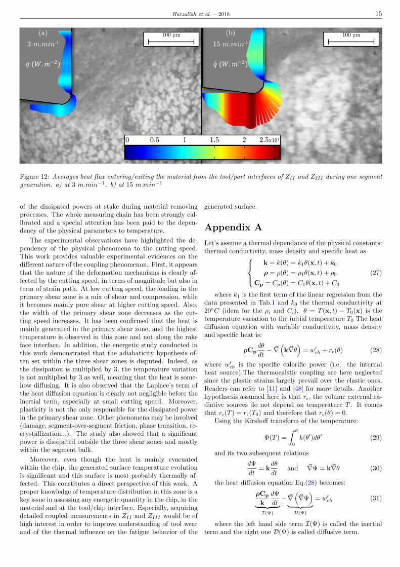
Zones II and III : The presented measurements mainlyfocused on the primary shear zone. Nonetheless they providevaluable information on other dissipatives zones (namely ZIIand ZIII). Indeed, from the thermal information it is possi-ble to assess the heat flux transfering between the tool andthe material. The Neumann boundary condition provides theincoming surface heat flux which can be compared to Eq.(21)as:

q = −k∂θ∂x

= βslηf · τf · Vsl − h(Tw − Ttool) (24)

Hence, evaluating the temperature gradient over the ma-terial frontier ∂Ω provides the heat fluxes depicted in Fig.12for both ZII and ZIII . It can be seen that the power gener-ated by friction in ZII is not sufficient to overcome the naturalflux heading from the hot segment toward the tool (cooler).It is also seen that increasing the cutting speed slightly in-creases the outbound heat flux. However, this increase is notproportional to the cutting speed and is to be matched withthe tool temperature (see Eq.(24)). Regarding Eq.(24), it canbe concluded that in ZII , the current tool temperature Ttoolis of the utmost importance for whoever wants to relate toolwear to the incoming thermal flux. Indeed, if Ttool is no longeran unknown variable, a given set of parameters βsl, ηf and hleads to a possible assessement of the last unknown variable:τf a key variable in machining operations.

In ZIII heat is entering the material, meaning that thegenerated surface is hot and slowly diffuses within the ma-terial. It is seen that the cutting speed strongly affects thesurface temperature beneath the tool which doubles between3 m.min−1 and 15 m.min−1 (approximatively 140C and300C). This ratio of 2 is also observed between the heatflux in ZIII depicted in Fig.12. No discontinuity is observedin the incoming flux which leads to consider that there is nocontact between the tool and the part along the clearanceface.

5.5 Global Powers

From a global stand point, it is worth recalling that the overallinput power of the cut is the cross product of the cutting forcewith the cutting speed and that the internal energy balancealows to write that:

W ′ext = Fc · Vc = −W ′int + K = W ′e +W ′a + K (25)

where K is the variation of kinetic energy, W ′int is the in-ternal power, W ′e the elastic power, W ′a the anelastic power,all being expressed in Watts. Hence, by neglecting the elas-tic power and K before the anelastic power, it is possible toevaluate the part of energy consumed in each of the threezones from the spatial intergation of the specific dissipationw′ch = βw′a depicted in Fig.8f and Fig.9f. It therefore comes:

W ′ext =d

β

∫⋃IV

i=I Zi

w′chdS (26)

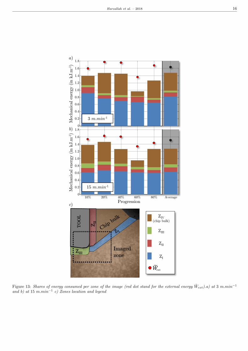
where d is the depth of cut, Zi is the surface area of thezones ZI , ZII and ZIII and ZIV is the remaining surface cor-responding to the imaged sub-surface of the sample and thebulk of the chip segment as depicted in Fig.13. The volumeintegration is performed under the strong assumption thatthe heat source is of homogeneous nature along the depthof the sample. Finally, dividing this quantity by the cuttingspeed results in obtaining Wext expressed in J.m−1; the en-ergy required to perform 1 meter of cut. Fig.13 depicts forthe 5 instants of each tests, the shares of energy consumedby each of the three zones (ZI , ZII , ZIII) and in the rest ofthe imaged area ZIV (denoted bulk & sub-surface in Fig.13).Various considerations can be made from such representation:

• As expected from the force measurements interpreta-tion, the overall consumed energy decreases as the cut-ting speed increases (which is consistant with classicaldynamometric observation).

• The dissipation in the segment bulk and in the sub-surface (i.e. outside of the three indentified and wellknown shear zones) is far from negligible. It is con-sistent with the strains measurments presented in theabove where it is seen that smaller but significant de-formation occurs within the bulk of the segment.

• The dissipation in the segment bulk suddenly dropswhen the crack propagation reaches completion (seeFig.13 progression 60% for both tests).

• The energy dissipated through plasticity in the sub-surface of ZII and ZIII slightly increases with the cut-ting speed, especially for ZIII . The interpretation of(Eq.23) leads to assume that the plastic deformation inthese zones also increases with the cutting speed.

• For most of the investigated instants, the internal en-ergy comes close to the external one. Meaning that mostof the energy is used within the captured area. How-ever, a part of the input energy is consumed outside ofthe image. Further investigations would be required tosort out if this energy is used to deform the subsurface(left of ZIII) or the top section of ZI both unseen fromthe imaging apparatus.

Conclusions and Perspectives

In this paper, the development and the implementation ofan original imaging apparatus dedicated to the simultaneousmeasurement of strain and temperature fields at small scale ispresented. The proposed experiment enables the monitoringof a 500× 500µm area at the tool tip using both visible andinfrared cameras. The study provides a novel and valuable in-sight to essential thermomechanical couplings and in-processmechanical phenomena involved in the generation of serratedchips and thus gives a new understanding of essential cuttingprocess mechanics occurring during the orthogonal cuttingof Ti-6Al-4V. The developed numerical post-processing alsoconstitutes an original contribution since it provides fieldsinformation at various time steps of the serrated chip gen-eration progression. Strain, strain-rates, temperatures, dis-sipated powers along with displacement, velocity and crackprogression are obtained at each pixel from both kinematicand thermal/energy measurement. It allows the assessment


3 m.min-1

100 µm 100 µm

0 1 2 1.5 2.5x107

0.5

15 m.min-1

𝑞 (𝑊.𝑚−2)

(b)

𝑞 (𝑊.𝑚−2)

(a)

3 m.min-1

Figure 12: Averages heat flux entering/exiting the material from the tool/part interfaces of ZII and ZIII during one segmentgeneration. a) at 3 m.min−1. b) at 15 m.min−1

of the dissipated powers at stake during material removingprocesses. The whole measuring chain has been strongly cal-ibrated and a special attention has been paid to the depen-dency of the physical parameters to temperature.

The experimental observations have highlighted the de-pendency of the physical phenomena to the cutting speed.This work provides valuable experimental evidences on thedifferent nature of the coupling phenomenon. First, it appearsthat the nature of the deformation mechanisms is clearly af-fected by the cutting speed, in terms of magnitude but also interm of strain path. At low cutting speed, the loading in theprimary shear zone is a mix of shear and compression, whileit becomes mainly pure shear at higher cutting speed. Also,the width of the primary shear zone decreases as the cut-ting speed increases. It has been confirmed that the heat ismainly generated in the primary shear zone, and the highesttemperature is observed in this zone and not along the rakeface interface. In addition, the energetic study conducted inthis work demonstrated that the adiabaticity hypothesis of-ten set within the three shear zones is disputed. Indeed, asthe dissipation is multiplied by 3, the temperature variationis not multiplied by 3 as well, meaning that the heat is some-how diffusing. It is also observed that the Laplace’s term ofthe heat diffusion equation is clearly not negligible before theinertial term, especially at small cutting speed. Moreover,plasticity is not the only responsible for the dissipated powerin the primary shear zone. Other phenomena may be involved(damage, segment-over-segment friction, phase transition, re-crystallization...). The study also showed that a significantpower is dissipated outside the three shear zones and mostlywithin the segment bulk.

Moreover, even though the heat is mainly evacuatedwithin the chip, the generated surface temperature evolutionis significant and this surface is most probably thermally af-fected. This constitutes a direct perspective of this work. Aproper knowledge of temperature distribution in this zone is akey issue in assessing any energetic quantity in the chip, in thematerial and at the tool/chip interface. Especially, acquiringdetailed coupled measurements in ZII and ZIII would be ofhigh interest in order to improve understanding of tool wearand of the thermal influence on the fatigue behavior of the

generated surface.

Appendix A

Let’s assume a thermal dependance of the physical constants:thermal conductivity, mass density and specific heat as

k = k(θ) = k1θ(x, t) + k0

ρ = ρ(θ) = ρ1θ(x, t) + ρ0

Cp = Cp(θ) = C1θ(x, t) + C0

(27)

where k1 is the first term of the linear regression from thedata presented in Tab.1 and k0 the thermal conductivity at20C (idem for the ρi and Ci). θ = T (x, t) − T0(x) is thetemperature variation to the initial temperature T0 The heatdiffusion equation with variable conductivity, mass densityand specific heat is:

ρCpdθ

dt− ~∇

(k~∇θ

)= w′ch + rε(θ) (28)

where w′ch is the specific calorific power (i.e. the internalheat source).The thermoealstic coupling are here neglectedsince the plastic strains largely prevail over the elastic ones.Readers can refer to [11] and [48] for more details. Anotherhypothsesis assumed here is that rε, the volume external ra-diative sources do not depend on temperature T . It comesthat rε(T ) = rε(T0) and therefore that rε(θ) = 0.

Using the Kirshoff transform of the temperature:

Ψ(T ) =

∫ θ

0

k(θ′)dθ′ (29)

and its two subsequent relations

dΨ

dt= k

dθ

dtand ~∇Ψ = k~∇θ (30)

the heat diffusion equation Eq.(28) becomes:

ρCp

k

dΨ

dt︸︷︷︸I(Ψ)

− ~∇(~∇Ψ)

︸︷︷︸D(Ψ)

= w′ch (31)

where the left hand side term I(Ψ) is called the inertialterm and the right one D(Ψ) is called diffusive term.


10% 20% 40% 60% 80% 0

0.2

0.4

0.6

0.8

1.0

1.2

1.4

1.6

Progression

Mec

hanic

al en

ergy (

in k

J.m

-1)

1.8

Average

0

0.2

0.4

0.6

0.8

1.0

1.2

1.4

1.6

Mec

hanic

al en

ergy (

in k

J.m

-1)

1.8 a)

ZIII

TO

OL

ZII

ZIV

(chip bulk)

ZIII

ZII

ZI

ext

3 m.min-1

15 m.min-1

b)

c)

Imaged

zone

Figure 13: Shares of energy consumed per zone of the image (red dot stand for the external energy Wext).a) at 3 m.min−1

and b) at 15 m.min−1 c) Zones location and legend


The key point here is that the available experimental datado not read the third dimension of the temperature fileds(along z). Indeed the thermal information is of surface na-ture and therefore requires to integrate the relation Eq.(31)over the z direction (through-thickness dimension). for thispurpose the through thickness average of fields varaibles mustbe defined as:

• =1

d

∫ d

0

•dz (32)

where d is the thickness of the sample (i.e. the depth ofcut). This imposes the set two main hypothesis [16]:

i) The calorific power w′ch is constant through thickness :w′ch = w′ch

ii) The heat conduction is much greater than the ther-mal losses (radiative and convective) of the front andback faces. It therefore comes that the averaged tem-perature through thickness can be approximated by themeasured surface temperature θ ≈ θ(z = 0) ≈ θ(z = d).

the integrated diffusive term then becomes:

D =1

d

∫ d

0

(∂2Ψ

∂x2+∂2Ψ

∂y2+∂2Ψ

∂z2

)dz

=1

d

∂2

∂x2

∫ d

0

Ψdz +1

d

∂2

∂y2

∫ d

0

Ψdz +1

d

[∂Ψ

∂z

]d0

=

[∂2Ψ

∂x2+∂2Ψ

∂y2

]+

1

d

[k∂θ

∂z

]d0

= ∆2Ψ +1

d

[k∂θ

∂z

]d0

(33)

where ∆2 is the two-dimensional Laplace operator such as

∆2Ψ = ~∇ ·(~∇Ψ)

= ~∇ ·(k(θ)~∇θ

)= ~∇ ·

(k1θ ~∇θ + k0

~∇θ)

= k1~∇ · θ ~∇θ + k0

~∇ · ~∇θ

= k1

(~∇θ · ~∇θ + ~∇ · ~∇θ × θ

)+ k0∆2θ

= k1

(~∇θ2 + ∆θ × θ

)+ k0∆2θ

= k1

(~∇θ)2

+ k∆2θ

(34)

and ∇ is here the two-dimensional gradient. The integratedinertial term I is expressed through the partial derivative ofΨ and the Liebniz intergration rule as:

I =1

d

∫ d

0

ρCp

k

dΨ

dtdz

=ρCp

kd

d

dt

∫ d

0

Ψdz

=ρCp

k

dΨ

dt

= ρCpdθ

dt

= ρCp

(∂θ

∂t+ ~v · ~∇θ

)(35)

where ~v = ~v(x, t) is the 2D velocity vector field. Finally,it should be noticed that the right hand side term of eq.(33)reads the boundary condition of the front and back faces ofthe sample. Therefore, assuming a convective/radiative con-ditions on these faces and an room temperature denoted Trthat equals the intitial temperature T0, one can write that:

−[k∂θ

∂z

]d0

= 2hθ + 2σε(T 4 − T 4r ) (36)

and the completed heat diffusion of the problem at instantt can be expressed as:

ρCp

(∂θ

∂t+ ~v · ~∇θ

)− k1

(~∇θ)2

− k∆2θ +2hθ

d+ . . .

2σε

d(T 4 − T 4

r ) = w′ch

(37)Remark: under such formalism, the use of a Stefan-

Boltzmann condition imposes to express the tempratures Tand Tr = T0 in Kelvin (and not in Celsius)

References

[1] Abaqus, Inc. ABAQUS Theory guide : version 6.12-1.Providence, RI, USA : ABAQUS, 2016.

[2] J.P. Arrazola, I. Arriola, and M.A. Davies. Analysis ofthe influence of tool type, coatings, and machinabilityon the thermal fields in orthogonal machining of AISI4140 steels. CIRP Annals - Manufacturing Technology,58:85–88, 2009.

[3] P.J. Arrazola, I. Arriola, M.A. Davies, A.L. Cooke, andB.S. Dutterer. The effect of machinability on thermalfields in orthogonal cutting of aisi 4140 steel. CIRP An-nals - Manufacturing Technology, 57:65–68, 2008.

[4] I. Arriola, E. Whitenton, J. Heigel, and P.J. Arrazola.Relationship between machinability index and in-processparameters during orthogonal cutting of steels. CIRPAnnals - Manufacturing Technology, 60:93–96, 2011.

[5] J. Artozoul, C. Lescalier, O. Bomont, and D. Dudzinski.Extended infrared thermography applied to orthogonalcutting. Applied Thermal Engineering, 64:441–452, 2014.

[6] T. Baizeau, S. Campocasso, G. Fromentin, F. Rossi, andG. Poulachon. Effect of rake angle on strain field dur-ing orthogonal cutting of hardened steel with c-bn tools.Procedia CIRP, 31:166–171, 2015.

[7] D. Basak, R.A. Overfelt, and D. Wang. Measurementof specific heat capacity and electrical resistivity of in-dustrial alloys using pulse heating techniques. Interna-tional Journal of Thermophysics, Vol. 24, No. 6, Novem-ber 2003, 24(6):1721–1733, 2003.

[8] L. Bodelot, E. Charkaluk, L. Sabatier, and P. Dufrenoy.Experimental study of heterogeneities in strain and tem-perature fields at the microstructural level of polycrys-talline metals through fully-coupled full-field measure-ments by digital image correlation and infrared thermog-raphy. Mechanics of Materials, 43(11):654 – 670, 2011.


[9] M. Boivineau, C. Cagran, D. Doytier, V. Eyraud, M. H.Nadal, B. Wilthan, and G. Pottlacher. Thermophysi-cal properties of solid and liquid ti-6al-4v (ta6v) alloy.International Journal of Thermophysics, 27(2):507–529,2006.

[10] M. Bornert, F. Bremand, P. Doumalin, M. Dupre, J-C. Fazzini, M. Grediac, F. Hild, S. Mistou, J. Molimard,J-J. Orteu, L. Robert, Y. Surrel, P Vacher, and B. Wat-trisse. Assessment of digital image correlation measure-ment errors: Methodology and results. Experimental Me-chanics, 49:353–370, 2008.

[11] T. Boulanger, A. Chrysochoos, C. Mabru, andA. Galtier. Calorimetric analysis of dissipative and ther-moelastic effects associated with the fatigue behaviorof steels. International Journal of Fatigue, 26:221–229,2004.

[12] J. Buda. New methods in the study of plastic deforma-tion in the cutting zone. CIRP Annals, 21:17–18, 1972.

[13] S.L. Cai, Y. Chen, G.G. Ye, M.Q. Jiang, Wang H.Y.,and L.H. Dai. Characterization of the deformation fieldin large-strain extrusion machining. Journal of MaterialsProcessing Technology, 216:48–58, 2015.

[14] M. Calamaz, D. Coupard, and F. Girot. A new mate-rial model for 2d numerical simulation of serrated chipformation when machining titanium alloy ti-6al-4v. In-ternational Journal of Machine Tools and Manufacture,48(3-4):275–288, 2008.

[15] M. Calamaz, D. Coupard, and F. Girot. Strain field mea-surement in orthogonal machining of a titanium alloy.Advanced Materials Research, 498:237–242, 2012.

[16] A. Chrysochoos and H. Louche. An infrared imageprocessing to analyse the calorific effects accompanyingstrain localisation. International Journal of EngineeringScience, 38:1759–1788, 2000.

[17] C. Courbon, T. Mabrouki, J. Rech, D. Mazuyer, F. Per-rard, and E. D’Eramo. Further insight into the chip for-mation of ferritic-pearlitic steels: Microstructural evo-lutions and associated thermo-mechanical loadings. In-ternational Journal of Machine Tools & Manufacture,77:34–46, 2014.

[18] M.A. Davies, A.L. Cooke, and E.R. Larsen. High band-width thermal microscopy of machining. CIRP Annals -Manufacturing Technology, 54(1):63–66, 2005.

[19] E.P. Gnanamanickam, S. Lee, J.P. Sullivan, and S. Chan-drasekar. Direct measurement of large-strain deforma-tion fields by particle tracking. Measurement science andtechnology, 20:095710 (12p), 2009.

[20] L. Gonzalez-Fernandez, E. Risueno, R.B. Perez-Saez,and M.J Tello. Infrared normal spectral emissivity ofti-6al-4v alloy in the 500 - 1150 k temperature range.Journal of Alloys and Compounds, 541:144–149, 2012.

[21] A. Guery, F. Hild, F. Latourte, and S. Roux. Slip activi-ties in polycrystals determined by coupling dic measure-ments with crystal plasticity calculations. InternationalJournal of Plasticity, 81:249–266, 2016.

[22] Y. Guo, M. Efe, W. Moscoso, D. Sagapuram, K.P. Trum-ble, and S. Chandrasekar. Deformation field in large-strain extrusion machining and implications for deforma-tion processing. Scripta Materialia, 66:235–238, 2012.

[23] Y. Guo, C. Saldana, W.D. Compton, and S. Chan-drasekar. Controlling deformation and microstructureon machined surfaces. Acta Materialia, 59:4538–4547,2011.

[24] B. Haddag, S. Atlati, M. Nouari, and M. Zenasni. Anal-ysis of the heat transfer at the tool-workpiece interfacein machining: determination of heat generation and heattransfer coefficients. Heat Mass Transfer, 51:1355–1370,2015.

[25] M. Harzallah, T. Pottier, J. Senatore, M. Mousseigne,G. Germain, and L. Landon. Numerical and exper-imental investigations of ti-6al-4v chip generation andthermo-mechanical couplings in orthogonal cutting. In-ternational Journal of Mechanical Sciences, 134(Supple-ment C):189 – 202, 2017.

[26] J.C. Heigel, E. Whitenton, B. Lane, M.A. Donmez,V. Madhavan, and W. Moscoso-Kingsley. Infrared mea-surement of the temperature at the tool-chip interfacewhile machining ti-6al-4v. Journal of Materials Process-ing Technology, 243:123–130, 2017.

[27] E. Heripre, M. Dexet, J. Crepin, L. Gelebart, A. Roos,M. Bornert, and D. Caldemaison. Coupling between ex-perimental measurements and polycrystal finite elementcalculations for micromechanical study of metallic mate-rials. International Journal of Plasticity, 23:1512–1539,2007.

[28] A. Hijazi and V. Madhavan. A novel ultra-high speedcamera for digital image processing applications. Mea-surement Science and Technology, 19(8):1–11, 2008.

[29] A. Icoz, L. Patriarca, M. Filippini, and Beretta S. Strainaccumulation in tial intermetallics via high-resolutiondigital image correlation (dic). Procedia Engineering,74:443–448, 2014.

[30] S.P.F. Jaspers and J. Dautzenberg. Material behaviourin metal cutting: Strains, strain rates and temperaturesin chip formation. Journal of Materials Processing Tech-nology, 121:123–135, 2002.

[31] Andrew Justice, Ibrahim Emre Gunduz, and Steven F.Son. Microscopic two-color infrared imaging of nial re-active particles and pellets. Thin Solid Films, 2016. The43rd International Conference on Metallurgical Coatingsand Thin Films.

[32] R.V. Kazban, K.M. Vernaza Pena, and J.J. Mason.Measurements of forces and temperature fields in high-speed machining. Experimental Mechanics, 48(3):307–317, 2008.

[33] F. Klocke, D. Lung, S. Buchkremer, and I. S. Jawahir.From orthogonal cutting experiments towards easy-to-implement and accurate flow stress data. Materials andManufacturing Processes, 28(11):1222–1227, 2013.


[34] R. Komanduri and R.H. Brown. On the mechanics ofchip segmentation in machining. Journal of engineeringfor industry, 103:33–51, 1981.

[35] R. Komanduri, T. Schroeder, J. Harza, B. Turkovich,and D. Flom. On the catastrophic shear instability inhigh-speed machining of an aisi 4340 steel. J. Eng. Ind.,104:121–131, 1982.

[36] F. Kone, Czarnota C., B. Haddag, and M. Nouari. Fi-nite element modelling of the thermo-mechanical behav-ior of coatings under extreme contact loading in dry ma-chining. Surface & Coatings Technology, 205:3559–3566,2011.

[37] T. Mabrouki and J.-F. Rigal. A contribution to a qual-itative understanding of thermo-mechanical effects dur-ing chip formation in hard turning. Journal of MaterialsProcessing Technology, 176:214–221, 2006.

[38] J.J. Mason, A.J. Rosakis, and G. Ravichandran. Onthe strain and strain rate dependence of the fraction ofplastic work converted into heat: an experimental studyusing high speed infrared detectors and the kolsky bar.Mechanics of Materials, 17:135–145, 1994.

[39] B. Pan, Z. Lu, and H. Xie. Mean intensity gradient: Aneffective global parameter for quality assessment of thespeckle patterns used in digital image correlation. Opticsand Lasers in Engineering, 48:469–477, 2010.

[40] B. Pan, H. Xie, Z. Wang, K. Qian, and Z. Wang. Studyon subset size selection in digital image correlation forspeckle patterns. Optics express, 16:7037–7048, 2008.

[41] Bing Pan, Wu Dafang, and Xia Yong. Incrementalcalculation for large deformation measurement usingreliability-guided digital image correlation. Optics andLasers in Engineering, 50:586–592, 2012.

[42] A. Perrier, F. Touchard, L. Chocinski-Arnault, andD. Mellier. Mechanical behaviour analysis of the inter-face in single hemp yarn composites: Dic measurementsand fem calculations. Polymer Testing, 52:1–8, 2016.

[43] J.-E. Pierre, J.-C. Passieux, J.-N. Perie, F. Bugarin, andL. Robert. Unstructured finite element-based digital im-age correlation with enhanced management of quadra-ture and lens distortions. Optics and Lasers in Engi-neering, 77:44 – 53, 2016.

[44] T. Pottier, G. Germain, M. Calamaz, A. Morel, andD. Coupard. Sub-millimeter measurement of finitestrains at cutting tool tip vicinity. Experimental Me-chanics, 54(6)(6):1031–1042., 2014.

[45] T. Pottier, H. Louche, S. Samper, H. Favreliere, F. Tou-ssaint, and P. Vacher. Proposition of a modal filteringmethod to enhance heat source computation within het-erogeneous thermomechanical problems. InternationalJournal of Engineering Science, 81:163–176, 2014.

[46] T. Pottier, M-P. Moutrille, J-B. Le-Cam, X. Balandraud,and M. Grediac. Study on the use of motion compensa-tion techniques to determine heat sources. Applicationto large deformations on cracked rubber specimens. Ex-perimental Mechanics, 49:561–574, 2009.

[47] N. Ranc, V. Pina, G. Sutter, and S. Philippon. Tempera-ture measurement by visible pyrometry: Orthogonal cut-ting application. J. Heat Transfer, 126(6):931–936, 2003.

[48] D. Rittel. On the conversion of plastic work to heatduring high strain rate deformation of glassy polymers.Mechanics of Materials, 31:131–139, 1999.

[49] M. Romano, M. Ryu, J. Morikawa, J.C. Batsale, andC. Pradere. Simultaneous microscopic measurements ofthermal and spectroscopic fields of a phase change mate-rial. Infrared Physics And Technology, 76:65 – 71, 2016.

[50] T. Sakagami, T. Nishimura, T. Yamaguchi, and N. Kubo.A new full-field motion compensation technique for in-frared stress measurement using digital image correla-tion. Jounal of Strain Analysis, 43:539–549, 2008.

[51] Thierry Sentenac and Remi Gilblas. Noise effect oninterpolation equation for neai infrared thermography.Metrologia, mar 2013.

[52] J.C. Stinville, M.P. Echlin, D. Texier, F. Bridier,P. Bocher, and T.M. Pollock. Sub-grain scale digitalimage correlation by electron microscopy for polycrys-talline materials during elastic and plastic deformation.Experimental Mechanics, 56(2):197 – 216, Feb 2016.

[53] S. Sun, M. Brandt, and M.S. Dargusch. Characteristicsof cutting forces and chip formation in machining of ti-tanium alloys. International Journal of Machine Toolsand Manufacture, 49(7):561 – 568, 2009.

[54] G. Sutter, L. Faure, A. Molinari, N. Ranc, and V. Pina.An experimental technique for the measurement of tem-perature fields for the orthogonal cutting oin high-speedmachining. International Journal of Machine Tools andManufacture, 43(7):671–678, 2003.

[55] Z. Tang, J. Liang, Z. Xiao, and C. Guo. Large deforma-tion measurement scheme for 3d digital image correlationmethod. Optics and Lasers in Engineering, 50(2):122–130, 2012.

[56] K. Triconnet, K. Derrien, F. Hild, and D. Baptiste. Pa-rameter choice for optimized digital image correlation.Optics and Lasers in Engineering, 47:728–737, 2009.

[57] Asier Ugarte, Rachid M’Saoubi, Ainhara Garay, and P.J.Arrazola. Machining behaviour of ti-6al-4v and ti-5553all0oys in interrupted cutting with pvd coated cementedcarbide. Procedia CIRP, 1:202 – 207, 2012. Fifth CIRPConference on High Performance Cutting 2012.

[58] P. Vacher, S. Dumoulin, F. Morestin, and S. Mguil-Touchal. Bidimensional strain measurement using digitalimages. Proc. Inst. Mech. Eng., 213:811–817, 1999.

[59] F. Valiorgue, A. Brosse, P. Naisson, J. Rech, H. Hamdi,and J-M. Bergheau. Emissivity calibration for temper-atures measurement using thermography in the contextof machining. Applied Thermal Engineering, 58:321–326,2013.

[60] Vincent Wagner, Arnaud Vissio, Emmanuel Duc, andMichele Pijolat. Relationship between cutting conditionsand chips morphology during milling of aluminium al-2050. The International Journal of Advanced Manufac-turing Technology, 82(9):1881–1897, Feb 2016.


[61] Qingqing Wang, Zhanqiang Liu, Bing Wang, QinghuaSong, and Yi Wan. Evolutions of grain size and micro-hardness during chip formation and machined surfacegeneration for ti-6al-4v in high-speed machining. TheInternational Journal of Advanced Manufacturing Tech-nology, 82(9):1725–1736, Feb 2016.

[62] J. Weng, P. Cohen, and M. Herniou. Camera calibrationwith distortion model and accuracy evaluation. IEEETransactions on Pattern Analysis and Machine Intelli-gence, 14(10):965–980, 1992.

[63] E.P. Whitenton. An introduction for machining re-searchers to measurement uncertainty sources in ther-mal images of metal cutting. International Journal ofMachining and Machinability of Materials, 12(3):195 –214, 2012.

[64] H. W. Yoon, D. W. Allen, and R. D. Saunders. Meth-ods to reduce the size-of-source effect in radiometers.Metrologia, 42:89–96, April 2005.

[65] F. Zemzemi, J. Rech, W. Ben Salem, A. Dogui,and P. Kapsa. Identification of a friction modelat tool/chip/workpiece interfaces in dry machining ofaisi4142 treated steels. Journal of Materials ProcessingTechnology, 209(8):3978 – 3990, 2009.

[66] D. Zhang, H. ZhaDing, and H. Ding. A study on the or-thogonal cutting mechanism based on experimental de-termined displacement and temperature fields. ProcediaCIRP, 46:35 – 38, 2016.

[67] X.P. Zhang, R. Shivpuri, and A.K. Srivastava. Role ofphase transformation in chip segmentation during highspeed machining of dual phase titanium alloys. Journalof Materials Processing Technology, 214(12):3048 – 3066,2014.

a coupled in-situ measurement of temperature and kinematic

Documents