a covariant approach to the quantisation of a rigid body … · for a rigid body according to the...
TRANSCRIPT
arX
iv:m
ath-
ph/0
5110
20v1
5 N
ov 2
005
A covariant approach to
the quantisation of a rigid body
Marco Modugno1, Carlos Tejero Prieto2, Raffaele Vitolo3
1Department of Applied Mathematics “G. Sansone”, University of Florence
Via S. Marta 3, 50134 Florence, Italy
email: [email protected]
2Department of Mathematics, University of Salamanca
Plaza de la Merced 1-4, 37008 Salamanca, Spain
email: [email protected]
3Department of Mathematics “E. De Giorgi”, University of Lecce
Via per Arnesano, 73100 Lecce, Italy
email: [email protected]
Preprint 2005.11.01. - 08.30.
Abstract
This paper concerns the quantisation of a rigid body in the framework of “co-variant quantum mechanics” on a curved spacetime with absolute time.
The basic idea is to consider the multi-configuration space, i.e. the configurationspace for n particles, as the n-fold product of the configuration space for one particle.Then we impose a rigid constraint on the multi-configuration space. The resultingspace is then dealt with as a configuration space of a single abstract ‘particle’. Thesame idea is applied to all geometric and dynamical structures.
We show that the above configuration space fits into the general framework of“covariant quantum mechanics”. Hence, the methods of this theory can be appliedto the rigid body.
Accordingly, we find exactly two inequivalent choices of quantum structures forthe rigid body. Then, we evaluate the quantum energy and momentum operatorsand the ‘rotational part’ of their spectra. We provide a new mathematical interpre-tation of two-valued wavefunctions on SO(3) in terms of single-valued sections of anew non-trivial quantum bundle. These results have clear analogies with spin.
Key words: Covariant classical mechanics, covariant quantum mechanics, rigid body.
1

2
MSC2000: 81S10,58A20,58C40,70G45,70E17,70H40,81Q10,81V55.
Acknowledgments
We would like to thank G. Besson, S. Gallot, A. Lopez Almorox, J. Marsden, G. Modugno,Mi. Modugno, L. M. Navas and D. Perrone, for useful discussions.
This work has been partially supported by MIUR, Progetto PRIN 2003 “Sistemi integra-
bili, teorie classiche e quantistiche”, GNFM and GNSAGA of INdAM, and the Universities of
Florence, Lecce and Salamanca.

Contents 3
Contents
Introduction 4
1 Covariant quantum mechanics 81.1 Classical scheme . . . . . . . . . . . . . . . . . . . . . . . . . . . . . . . . . 81.2 Quantum scheme . . . . . . . . . . . . . . . . . . . . . . . . . . . . . . . . 10
2 Rigid body classical mechanics 142.1 One–body mechanics . . . . . . . . . . . . . . . . . . . . . . . . . . . . . . 142.2 Multi-body mechanics . . . . . . . . . . . . . . . . . . . . . . . . . . . . . 15
2.2.1 Configuration space . . . . . . . . . . . . . . . . . . . . . . . . . . . 152.2.2 Center of mass splitting . . . . . . . . . . . . . . . . . . . . . . . . 162.2.3 Multi–electromagnetic field . . . . . . . . . . . . . . . . . . . . . . . 18
2.3 Rigid body mechanics . . . . . . . . . . . . . . . . . . . . . . . . . . . . . 192.3.1 Configuration space . . . . . . . . . . . . . . . . . . . . . . . . . . . 192.3.2 Rotational space . . . . . . . . . . . . . . . . . . . . . . . . . . . . 202.3.3 Tangent space of rotational space . . . . . . . . . . . . . . . . . . . 222.3.4 Induced metrics . . . . . . . . . . . . . . . . . . . . . . . . . . . . . 242.3.5 Induced connection . . . . . . . . . . . . . . . . . . . . . . . . . . . 272.3.6 Induced electromagnetic field . . . . . . . . . . . . . . . . . . . . . 272.3.7 Spacetime structures . . . . . . . . . . . . . . . . . . . . . . . . . . 302.3.8 Dynamical functions . . . . . . . . . . . . . . . . . . . . . . . . . . 30
3 Rigid body quantum mechanics 323.1 Quantum structures . . . . . . . . . . . . . . . . . . . . . . . . . . . . . . 323.2 Quantum dynamics . . . . . . . . . . . . . . . . . . . . . . . . . . . . . . . 34
4 Rotational quantum spectra 374.1 Angular momentum in the free case . . . . . . . . . . . . . . . . . . . . . . 374.2 Energy in the free case . . . . . . . . . . . . . . . . . . . . . . . . . . . . . 384.3 Spectra with electromagnetic field . . . . . . . . . . . . . . . . . . . . . . . 42
References 44

4 Contents
Introduction
A covariant formulation of classical and quantum mechanics on a curved spacetimewith absolute time based on fibred manifolds, jets, non linear connections, cosymplecticforms and Frolicher smooth spaces has been proposed by A. Jadczyk and M. Modugno [28,29] and further developed by several authors (see, for instance, [8, 30, 31, 34, 53, 61, 48]).We shall briefly call this approach “covariant quantum mechanics”. It presents analogieswith geometric quantisation (see, for instance, [18, 20, 40, 56, 55, 62] and referencestherein), but several novelties as well. In fact, it overcomes typical difficulties of geometricquantisation such as the problem of polarisations; moreover, in the flat case, it reproducesthe standard quantum mechanics, hence it allows us to recover all classical examples (see[48] for a comparison between the two approaches).
Here, we discuss an original geometric formulation of classical and quantum mechanicsfor a rigid body according to the general scheme of “covariant quantum mechanics”. Ourmethod, based on the classical multi–body and rigid model developed in detail in [49]and on the covariant quantum mechanics, seems to be a new approach, which is able tounify different cases on a clean mathematical scheme.
We start with a sketch of the essential features of the general “covariant quantummechanics” following [29, 31, 32, 61]. The classical theory is based on a fibred manifold(“spacetime”) over time, equipped with a vertical Riemannian metric (“space–like met-ric”), a certain time and metric preserving linear connection (“gravitational connection”)and a closed 2–form (“electromagnetic field”). The above objects yield a cosymplectic 2–form on the first jet space of spacetime (“phase space”), in the sense of [13]. This 2–formcontrols the classical dynamics. The quantum theory is based on a Hermitian line bun-dle over spacetime (“quantum bundle”) equipped with a Hermitian universal connection,whose curvature is proportional to the above classical cosymplectic 2-form. This quantumstructure yields in a natural way a Lagrangian (hence the dynamics) and the quantumoperators.
In view of the formulation of classical mechanics of a rigid body in the framework ofthe above scheme, we proceed in three steps [49].
Namely, we start with a flat spacetime for a pattern one–body mechanics.Then, we consider an n-fold fibred product of the pattern structure as multi-spacetime
for the n-body mechanics. A geometric ‘product space’ for n-body mechanics has beendeveloped by several authors in different ways (see, for instance, [12, 14, 44, 29, 49]. Inparticular, our approach is close to that in [12] for the ‘rotational’ part of the rigid bodydynamics, it can be easily compared with [45], and is close to [14] for the formulation ofquantum structures.
Moreover, we consider the subbundle of the multi–spacetime induced by a rigid con-straint as configuration space for the rigid body mechanics. We can prove that this con-figuration space fulfills the requirements of the spacetime assumed in “covariant quantummechanics”; hence, the general machinery of covariant classical and quantum mechanicscan be easily applied to the rigid body.

Contents 5
Next, we proceed with the quantisation of the rigid body. We discuss the existenceand classification of the inequivalent quantum structures over the rigid configurationspace. Quantum structures are pairs consisting of a hermitian complex line bundle and ahermitian connection on it whose curvature is proportional to the cosymplectic 2-form. Itturns out that there are two possible quantum bundles: a trivial and a non trivial one. Thetransition functions of the non-trivial bundle are constant, hence both the trivial and thenon-trivial bundle are endowed with a flat hermitian connection. Such connections can bedeformed by adding the classical Poincare–Cartan form to produce two non-isomorphicquantum structures.
Then, we evaluate the classical ‘translational’ and ‘rotational’ observables of position,momenta ad energy and the corresponding quantum operators.
Finally, we explicitly compute the spectra of the rotational momentum and energyquantum operators for all quantum structures, in the case of vanishing electromagneticfield (‘free’ rigid body). The computations existing in the literature for the spectra of arigid body in some special electromagnetic fields can be recovered in our scheme analo-gously to the previous procedure by means of the quantum structure associated with thetrivial quantum bundle (see, for instance, [1, 2, 3, 4, 7, 9, 10, 11, 16, 21, 23, 25, 26, 27,36, 39, 41, 42, 43, 46, 47, 50, 51, 52, 54, 57, 58, 59, 60]).
The non-trivial quantum structure is an original feature of our paper in the frameworkof covariant quantum mechanics; for a similar result from the viewpoint of geometricquantisation, see [58]. The non-trivial quantum bundle provides a clear mathematicalsetting and interpretation of the double–valued wavefunctions formalism. Indeed, severalauthors have consider double–valued wavefunctions (see, for instance, [3, 7, 11, 21, 41, 47,50]). Sometimes [11, 47], these functions have been discarded because they are supposedto break the continuity of the quantum rotation operator. However, in our approach, nocontinuity is broken if we allow the existence of a non trivial quantum bundle. Schrodingerrefused to consider double-valued wavefunctions. But by some authors [37] is was arguedthat the probability density must be single valued, hence double-valued wavefunctionsmust be accepted because their square is single-valued.
However, the most important contribution on this problem was given by Casimir inhis Ph.D. thesis [9]. On p. 72 Casimir explains that the two-valuedness is due to thenon-contractibility of the space of rotations:
. . . To a curve connecting ξ , η , ζ , χ with −ξ , −η , −ζ , −χ there corre-sponds a closed motion that cannot be contracted; it may be changed into arotation through 2π . Accordingly, we may say: the two-valuedness of the ξi[coordinates on R4 restricted to S3 ], . . . , the possibility of two-valued rep-resentations, are based on the kinematical fact that a 2π rotation cannot becontracted.
In our opinion, our non-trivial quantum bundle is a modern topological model imple-menting the above features: it appears exactly because the fundamental group of SO(3)is Z2 .
6 Contents
As far as we know, in all cases in which the spectrum of molecules has half–integereigenvalues, this value can be attributed to the spin of constituent particles. It meansthat nature chooses always, by a superselection rule, the trivial bundle. On the otherhand, our scheme foresees the non trivial bundle as another theoretical possibility. Evenif this one seems to have no actual physical reality, it could be taken as basis for a kind of“semi–classical model of spin”, by taking into account the scheme of covariant quantummechanics for a spin particle [8]. Indeed, some authors have considered such a possibility,by following other approaches (see, for instance [3, 7, 21, 24]).
In this paper we compute spectra only with respect to a fixed inertial observer. How-ever, as a by-product of the covariant approach to quantum rigid systems, we couldcompute spectra also with respect to accelerated observers. In experiments it often hap-pens that spectra come from sources which do not have inertial motion with respect tothe laboratory. It is customary to add ad hoc terms to the standard Schrodinger oper-ator in order to fit most spectral lines. Our framework allows one to obtain covariantSchroedinger operators with respect to accelerated frames. Hence, in principle, it shouldbe possible to compute explicitly (possibly by means of numerical analysis techniques)the spectra. But this issue is left to future investigations.
In this paper we will not touch the issue of reduction. In particular, it would be in-teresting to check if the Guillemin–Sternberg conjecture [22] (see also [19]) holds in thecase of a free rigid body. (We recall that the Guillemin–Sternberg conjecture states thecommutation between the reduction and the quantization procedures.) In fact, the groupSO(3) acts as a group of symmetries on a free rigid body. A cosymplectic reduction pro-cedure (analogous to the Marsden–Weinstein reduction procedure) could be formulated.A similar analysis has been carried out in [36] in order to formulate a geometric prequan-tization (see also [52] for similar results under stronger hypotheses). The coadjoint orbitsof constant angular momentum turn out to be spheres S2 . It would be very interestingto investigate the interplay between the two inequivalent quantum structures of the rigidbody and the possible quantum structures of coadjoint orbits, especially in view of thefact that their topologies are different. But this will be the subject of future work.
From a physical viewpoint, our model can describe extremely cold molecules. In fact,vibrational modes are of great importance in quantum dynamics, unless the temperatureis extremely low. A different approach to the quantisation of a rigid body is providedby the so called ‘pseudo-rigid body’ [16, 44, 60], by considering a potential with suitablewells confining bodies to be near to a rigid constraint. This approach seems to be morephysical than ours, but it is more complicated. Indeed, we think that our approach can beconsidered a useful model, due to its simplicity. Even in the purely classical descriptionof rigid bodies one can follow two ways: i) a more physical but very complicated one,by considering forces bounding the constituent particles and by referring to the limitcase when these forces freeze the distances between the particles; ii) a more ideal andmuch simpler one, by considering the rigid constrained body, regardless of the physicalorigin of the constraint. The scheme of covariant quantum mechanics allows us to apply a

Contents 7
viewpoint analogous to the second approach mentioned above to the quantum mechanicsof a “rigid body”.
We assume manifolds and maps to be C∞ . If M and N are manifolds, then the sheafof local smooth maps M → N is denoted by map(M , N) .

8 1 Covariant quantum mechanics
1 Covariant quantum mechanics
We start with a brief sketch of the basic notions of “covariant quantum mechan-ics”, paying attention just to the facts that are strictly needed in the present paper.We follow [29, 31, 32, 33, 35, 53, 61]. For further details and discussions the readershould refer to the above literature and references therein.
In order to make classical and quantum mechanics explicitly independent from scales,we introduce the “spaces of scales”. Roughly speaking, a space of scales has the algebraicstructure of IR+ but has no distinguished ‘basis’. The basic objects of our theory (metric,electromagnetic field, etc.) will be valued into scaled vector bundles, that is into vectorbundles twisted with spaces of scales. We shall use rational tensor powers of spaces ofscales. In this way, each tensor field carries explicit information on its “scale dimension”.
Actually, we assume the following basic spaces of scales: the space of time intervals
T , the space of lengths L , the space of masses M .We assume the Planck’s constant ~ ∈ T∗ ⊗ L2 ⊗ M . Moreover, a particle will be
assumed to have a mass m ∈ M and a charge q ∈ T∗ ⊗ L3/2 ⊗ M1/2 .
1.1 Classical scheme
G.1 Assumption. We assume:- the time to be an affine space T associated with the vector space T := T ⊗ IR ,- the spacetime to be an oriented manifold E of dimension 1 + 3 ,- the time fibring to be a fibring (i.e., a surjective submersion) t : E → T ,- the spacelike metric to be a scaled vertical Riemannian metric
g : E → L2 ⊗ S2V ∗E ,
- the gravitational connection to be a linear connection of spacetime
K : TE → T ∗E ⊗TE
TTE ,
such that ∇[K]dt = 0 and ∇[K]g = 0 , and whose curvature R[K] is “vertically sym-metric”,
- the electromagnetic field to be a closed scaled 2–form
F : E → (L1/2 ⊗ M1/2) ⊗ Λ2T ∗E .
The spacelike orientation and the metric g yield the spacelike scaled volume form ηand its dual η .
With reference to a given particle with mass m and charge q , it is convenient toconsider the rescaled sections
G := m~ g : E → T ⊗ S2V ∗E and q
~ F : E → Λ2T ∗E .

1.1 Classical scheme 9
We shall refer to fibred charts (x0, xi) of E , where x0 is adapted to the affine structureof T and to a time scale u0 ∈ T . Latin indices i, j, . . . and Greek indices λ, µ, . . . willlabel space–like and spacetime coordinates, respectively. For short, we shall denote theinduced dual bases of vector fields and forms by ∂λ and dλ . The vertical restriction offorms will be denoted by the check “ ∨ ” .
We have the coordinate expression G = G0ij u0 ⊗ di ⊗ dj . The coordinate expression
of the condition of vertical symmetry of R[K] is Riλjµ = R
jµiλ .
A motion is defined to be a section s : T → E .
We assume the first jet space of motions J1E as phase space for classical mechanics ofa spinless particle; the first jet prolongation j1s of a motion s is said to be its velocity . Wedenote by (xλ, xi
0) the chart induced on J1E . We shall use the natural complementarymaps d : J1E × T → TE and θ : J1E ×E TE → VE , with coordinate expressionsd = u0 ⊗ (∂0 + xi
0 ∂i) and θ = (di − xi0 d
0) ⊗ ∂i . We set θi ≡ di − xi0 d
0 .
An observer is defined to be a (local) section o : E → J1E .
An observer o is said to be rigid if the Lie derivative L[o] g vanishes.
Let us consider an observer o .
A chart (x0, xi) is said to be adapted to o if oi0 ≡ xi
0 o = 0 . We obtain the mapsν[o] : TE → VE : X → X − o ydt(X) and ∇[o] : J1E → T∗ ⊗ VE : e1 − o(e) . We definethe observed component of a vector v ∈ TE , to be the spacelike vector ~v[o] := ν[o](v) .Accordingly, if s is a motion, then we define the observed velocity to be the section∇[o] j1s : T → T∗ ⊗ VE .
We define the observed kinetic energy and momentum, respectively, as the maps
K[o] := 12G(∇[o],∇[o]) : J1E → T ∗E and Q[o] := θ∗ G(∇[o]) : J1E → T ∗E ,
with coordinate expressions K[o] = 12G0
ij xi0 x
j0 d
0 and Q[o] = G0ij x
j0 θ
i .
We define the magnetic field and the observed electric field , respectively, as
~B := 12i(
∨
F )η and ~E[o] := −o yF .
Then, we obtain the observed splitting
F = −2dt ∧ ~E[o] + 2ν∗[o](i( ~B)η
).
The linear connection K yields an affine connection Γ of the affine bundle J1E → E ,with coordinate expression Γ
λi00µ = K
λiµ , and the non linear connection γ := d yΓ :
J1E → T∗ ⊗ TJ1E of the fibred manifold J1E → T , with coordinate expression γ =u0 ⊗ (∂0 + xi
0 ∂i + γ0i0 ∂
0i ) , where γ
0i0 := K
hik x
h0 x
k0 + 2K
hi0 x
h0 + K
0i0 . Moreover,
Γ yields the 2–form Ω := G(ν[Γ] ∧ θ) : J1E → Λ2T ∗J1E . We have the coordinateexpression Ω = G0
ij (di0 − γ
0i0 d
0 − Γh
i0 θ
h) ∧ θj , where Γh
i0 ≡ Γ
hi00k x
k0 + Γ
hi000 . The
2–form Ω turns out to be closed, in virtue of the assumed symmetry of R[K] , and non

10 1 Covariant quantum mechanics
degenerate as dt∧Ω ∧Ω ∧Ω is a scaled volume form of J1E . Thus, Ω turns out to bea cosymplectic form.
There is a natural geometric way to “merge” the gravitational and electromagneticobjects into joined objects, in such a way that all mutual relations holding for gravitationalobjects are preserved for joined objects. Later on, we shall refer to such joined objectsand we can forget about the two component fields, in many respects. In particular, wedeal with the joined 2–form Ω := Ω + 1
2q~F and the joined connection γ = γ + γe ,
where γe turns out to be the Lorentz force γe = −G♯∨
(d yF ) .We obtain dΩ = 0 and dt ∧Ω ∧ Ω ∧Ω = dt ∧Ω ∧Ω ∧ Ω . Thus, also Ω turns out to
be a cosymplectic form.The joined 2–form Ω rules the classical dynamics in the following way.The closed form Ω admits local “horizontal” potentials of the type A↑ : J1E → T ∗E ,
whose coordinate expression is of the type A↑ = −(12G0
ij xi0 x
j0 −A0) d
0 + (G0ij x
j0 +Ai) d
i ,that is, for each observer o , of the type A↑ = −K[o] + Q[o] + A[o] , where A[o] := o∗A↑ :E → T ∗E .
We define the (local) Lagrangian L[A↑] := d yA↑ : J1E → T ∗E and the (local) mo-
mentum P[A↑] := θ∗VEL[A↑] : J1E → T ∗E , with expressions L[A↑] = (12G0
ij xi0 x
j0 +
Ai xi0 + A0) d
0 and P[A↑] = (G0ij x
j0 + Ai) θ
i . Indeed, the Poincare–Cartan form Θ =L[A↑] + P[A↑] associated with L[A↑] turns out to be just A↑ .
Moreover, given an observer o , we define the (observed) Hamiltonian H[A↑, o] :=−o yA↑ : J1E → T ∗E and the (observed) momentum P[A↑, o] := ν[o] yA↑ : J1E →T ∗E , with coordinate expressions H[A↑, o] = (1
2G0
ij xi0 x
j0−A0) d
0 and P[A↑, o] = (G0ij x
j0+
Ai) di , in adapted coordinates. We obtain also the scaled function ‖P[A↑, o]‖2 , with co-
ordinate expression ‖P[A↑, o]‖20 = G0
ij xi0 x
j0 + 2Ai x
i0 +Gij
0 AiAj .The Euler–Lagrange equation, in the unknown motion s , associated with the (local)
Lagrangians L[A↑] turns out to be the global equation ∇[γ]j1s = 0 , that is ∇[γ]j1s =γe j1s . This equation is just the generalised Newton’s equation of motion for a chargedparticle in the given gravitational and electromagnetic field. We assume this equation tobe our classical equation of motion.
1.2 Quantum scheme
A quantum bundle is defined to be a complex line bundle Q → E , equipped with aHermitian metric h with values in C⊗Λ3V ∗E . A quantum section Ψ : E → Q describesa quantum particle.
A local section b : E → L3/2 ⊗ Q , such that h(b,b) = η , is a local basis. We denotethe local complex dual basis of b by z : Q → L∗3/2 ⊗ C . If Ψ is a quantum section, thenwe write locally Ψ = ψb , where ψ := z Ψ : E → L∗3/2 ⊗ C .
The Liouville vector field is defined to be the vector field I : Q → VQ : q 7→ (q, q) .Lets us consider the phase quantum bundle Q↑ := J1E ×E Q → J1E .If Q[o] is a family of Hermitian connections of Q → E parametrised by the observers
o , then there is a unique Hermitian connection Q↑ of Q↑ → J1E , such that Q[o] = o∗Q↑ ,

1.2 Quantum scheme 11
for each observer o . This connection is called universal and is locally of the type Q↑ =χ↑[b] + iA↑[b] ⊗ I↑ , where χ↑[b] is the flat connection induced by a local quantum basisb and A↑[b] is a local horizontal 1–form of J1E . The map Q[o] 7→ Q↑ is a bijection.
We define a phase quantum connection to be a connection Q↑ of the phase quantumbundle, which is Hermitian, universal and whose curvature is R[Q↑] = −2 iΩ ⊗ I↑ .
A phase quantum connection Q↑ is locally of the type Q↑ = χ↑[b]+ iA↑[b]⊗I↑ , whereA↑[b] is a local horizontal potential for Ω .
We remark that the equation dΩ = 0 turns out to be just the Bianchi identity for aphase quantum connection Q↑ .
A pair (Q,Q↑) is said to be a quantum structure.
Two quantum bundles Q1 and Q2 on E are said to be equivalent if there exists anisomorphism of Hermitian line bundles f : Q1 → Q2 over E (the existence of suchan f is equivalent to the existence of an isomorphism of line bundles). Two quantumstructures (Q1,Q
↑1) and (Q2,Q
↑2) , are said to be equivalent if there exists an equivalence
f : Q1 → Q2 which maps Q↑1 into Q↑
2 .
A quantum bundle is said to be admissible if it admits a phase quantum connection.Actually, the following results holds.
Let us consider the cohomology H∗(E, X) with values in X = IR , or X = Z , theinclusion morphism i : Z → IR and the induced group morphism i∗ : H∗(E,Z) →H∗(E, IR) .
The difference of two local horizontal potentials for Ω turns out to be a locally closedspacetime form. Therefore, we can prove that the de Rham class [Ω]R naturally yields acohomology class [Ω] ∈ H2(E, IR) .
1.1 Proposition. [61] We have the following classification results.
1) The equivalence classes of complex line bundles on E are in bijection with the 2ndcohomology group H2(E,Z) .
2) There exists a quantum structure on E , if and only if
[Ω] ∈ i2(H2(E,Z)
)⊂ H2(E, IR) ≃ H2(J1E, IR) .
3) Equivalence classes of quantum structures are in bijection with the set
(i2)−1([Ω]) × H1(E, IR)/H1(E,Z) .
More precisely, the first factor parametrises admissible quantum bundles and the sec-ond factor parametrises phase quantum connections.
The quantum theory is based on the only assumption of a quantum structure, sup-posing that the background spacetime admits one.
G.2 Assumption. We assume a quantum bundle Q equipped with a phase quantumconnection Q↑ .
12 1 Covariant quantum mechanics
All further quantum objects will be derived from the above quantum structure bynatural procedures.
We have been forced to assume that Q↑ lives on the phase quantum bundle Q↑ becauseof the required link with the 2–form Ω . On the other hand, in order to accomplish thecovariance of the theory, we wish to derive from Q↑ new quantum objects, which areobserver independent, hence living on the quantum bundle. For this purpose we follow asuccessful projectability procedure: if V ↑ → J1E is a vector bundle which projects on avector bundle V → E , then we look for sections σ↑ : J1E → V ↑ which are projectableon sections σ : E → V and take these σ as candidates to represent quantum objects.
The quantum connection allows us to perform covariant derivatives of sections of Q
(via pullback). Then, given an observer o , the observed quantum connection
Q[o] := o∗Q↑ yields, for each section Ψ : E → Q , the observed quantum differential
and the observed quantum Laplacian, with coordinate expressions
o
∇λ ψ = (∂λ − iAλ)ψ ,
o
∆0 ψ =(Ghk
0 (∂h − iAh)(∂k − iAk) +∂h(G
hk0
√|g|)
√|g|
(∂k − iAk))ψ .
We can prove that all 1st order covariant quantum Lagrangians [31] are of the type(we recall that m/~ has been incorporated into G and A[o])
L[Ψ] = 12
(i (ψ ∂0ψ − ψ ∂0ψ) + 2A0 ψ ψ
−Gij0 (∂iψ ∂jψ + AiAj ψ ψ) − iAi
0 (ψ ∂iψ − ψ ∂iψ) + k ρ0 ψ ψ) √
|g| d0 ∧ d1 ∧ d2 ∧ d3 ,
where ρ0 = Gij0 Rhi
hj is the scalar curvature of the spacetime connection K and k ∈ IR is
an arbitrary parameter (which cannot be determined by covariance arguments).By a standard procedure, these Lagrangians yield the quantum momentum, the Euler–
Lagrange operator (generalised Schrodinger operator) and a conserved form (probabilitycurrent). We assume the quantum sections Ψ to fulfill the generalised Schrodinger equa-tion with coordinate expression (we recall that m/~ has been incorporated into G andA[o])
S0 ψ =( o
∇0 + 12
∂0
√|g|
√|g|
− 12
i (o
∆0 + k ρ0))ψ = 0 .
Next, we sketch the formulation of quantum operators.We can exhibit a distinguished Lie algebra spec(J1E) ⊂ map(J1E, IR) of functions,
called special phase functions , of the type f = f 0 12G0
ij xi0 x
j0 +f iG0
ij xj0 + f , where fλ, f ∈
map(E, IR) . Among special phase functions we have xλ , Pj , H0 and ‖P‖20 . The bracket
of this algebra is defined in terms of the Poisson bracket and γ .Then, by classifying the vector fields on Q which preserve the Hermitian metric and
are projectable on E and on T , we see that they constitute a Lie algebra, which is

1.2 Quantum scheme 13
naturally isomorphic to the Lie algebra of special phase functions. These vector fields canbe regarded as pre–quantum operators Z[f ] acting on quantum sections.
The sectional quantum bundle is defined to be the bundle Q → T , whose fibres Qτ ,with τ ∈ T , are constituted by smooth quantum sections, at the time τ , with compactsupport. This infinite dimensional complex vector bundle turns out to be F–smooth inthe sense of Frolicher [17] and inherits a pre–Hilbert structure via integration over thefibres. A Hilbert bundle can be obtained by completion.
We can prove that the Schrodinger operator S can be naturally regarded as a linearconnection of Q → T .
Eventually, a natural procedure associates with every special phase function f a sym-metric quantum operator f : Q → Q , fibred over T , defined as a linear combination ofthe corresponding pre–quantum operator Z[f ] and of the operator f 0 S0 . We obtain thecoordinate expression (we recall that m/~ has been incorporated into G and A[o])
fψ =(f − i fh (∂h − iAh) − i 1
2
∂h(fh√|g|)
√|g|
− 12f 0(
o
∆0 + k ρ0))ψ .
For example, we have
x0 ψ = x0 ψ , xi ψ = xi ψ ,
Pj ψ = −i (∂j + 12
∂j
√|g|
√|g|
)ψ , H0 ψ =(− 1
2(
o
∆0 + k ρ0) − A0
)ψ ,
‖P‖20 ψ =
(−Gij
0 AiAj − i∂h(A
h0
√|g|)
√|g|
− 2 i Ah0 ∂h − (
o
∆0 + k ρ0))ψ .
14 2 Rigid body classical mechanics
2 Rigid body classical mechanics
Now, we consider a rigid body and show how it can be quantised according tothe scheme of the above general theory.
The configuration space of the classical rigid body is formulated in three stepsaccording to [49]:
- we start with a flat “pattern spacetime” of dimension 1+3 for the formulationof one–body classical and quantum mechanics;
- then, we consider the n–fold fibred product of the pattern spacetime, equippedwith the induced structures, as the framework for n–body classical and quantummechanics;
- finally, we consider the rigid constrained fibred submanifold of the above n–fold fibred product along with the induced structures, as the framework for classicalrigid–body.
Then, we show that this configuration space fits the general setting of “covariantquantum mechanics” sketched in the previous section. Hence, that general schemecan be applied to this specific case.
2.1 One–body mechanics
Following the general scheme, we start by assuming a flat spacetime for one–body mechanics, which is called the pattern spacetime. All objects related to thispattern spacetime are called pattern objects
Let us consider a system of one particle, with mass m and charge q .
We assume as pattern spacetime a (1+3)–dimensional affine space E , associated withthe vector space E and equipped with an affine map t : E → T as time map.
From the above affine structure follow some immediate consequences.
The map Dt : E → T yields the 3–dimensional vector subspace S := Dt−1(0) ⊂E and the 3–dimensional affine subspace U := (id[T∗] ⊗ Dt)−1(1) ⊂ T∗ ⊗ E , which isassociated with the vector space T∗ ⊗ S .
Thus, t : E → T turns out to be a principal bundle associated with the abelian groupS . Moreover, we have the natural isomorphisms TE ≃ E × E , VE ≃ E × S andJ1E ≃ E × U .
We assume a Euclidean metric g ∈ L2⊗ (S∗⊗S∗) as a spacelike metric. Moreover, weassume the connection K induced by the affine structure as the gravitational connection.Furthermore, we assume an electromagnetic field F .
Thus, we obtain dΩ = 0 and dF = 0 . Moreover, because of the affine structureof spacetime, Ω and F turn out to be globally exact. We denote the global potentials(defined up to a constant) for Ω and F by A↑ and Ae .
We recall also the obvious natural action of the group O(S, g) on S .
A motion s and an observer o are said to be inertial if they are affine maps. Anyinertial observer yields a splitting of the type E ≃ T × P [o] , where P [o] is an affine

2.2 Multi-body mechanics 15
space associated with S . Any inertial motion yields an inertial observer o and an affineisomorphism P [o] ≃ S .
For each inertial observer o , we obtain the splitting A↑ = −K[o]+Q[o]+A[o] , whereA[o] ∈ E
∗is a constant 1–form.
2.2 Multi-body mechanics
We can describe the classical mechanics of a system of n particles moving in agiven gravitational and electromagnetic field by representing this system as a one–body moving in a higher dimensional spacetime equipped with suitable fields whichfulfill the same properties postulated for the standard spacetime.
In this way, we can use for a system of n particles all concepts and resultsobtained for a one–body.
2.2.1 Configuration space
We assume as configuration space for a system of n particles the n–fold fibredproduct of the pattern spacetime, called “multi–spacetime”. Then, the metric field,gravitational field and electromagnetic field naturally equip this multi–spacetimewith analogous “multi” fields.
Thus, the structure of multi–spacetime is analogous to that of pattern spacetime.The different dimension of the fibres in the two cases has no importance in manyrespects; hence, most concepts and results can be straightforwardly translated fromthe pattern case to the multi–case. Indeed, the multi–fields involve suitable weightsrelated to the masses and charges of the particles, in such a way that the mechanicalequations arising from the multi–approach coincide with the system of equationsfor the single particles.
So, we can formulate the classical mechanics of an n-body analogously to thatof a one–body equipped with the total mass and affected by the given multi–metric,multi–gravitational field and multi–electromagnetic field.
On the other hand, the multi–spacetime is equipped with the projections of thefibred product, which provide additional information concerning each particle.
All objects related to this multi–spacetime are called multi–objects and labelledby the subscript “mul” .
Let us consider a system of n particles, with n ≥ 2 , and with masses m1, . . . , mn andcharges q1, . . . , qn .
Then, we define the total mass m :=∑
imi , the i-th weight µi := mi/m ∈ IR+ andthe total charge q :=
∑i qi . Of course, we have
∑i µi = 1 .
In order to label the different particles of the system, we introduce n identical copies ofthe pattern objects Ei ≡ E , Si ≡ S , U i ≡ U , gi ≡ g , Fi ≡ F , for i = 1, . . . , n .
We assume the fibred product over T
Emul := E1 ×T. . .×
TEn ,
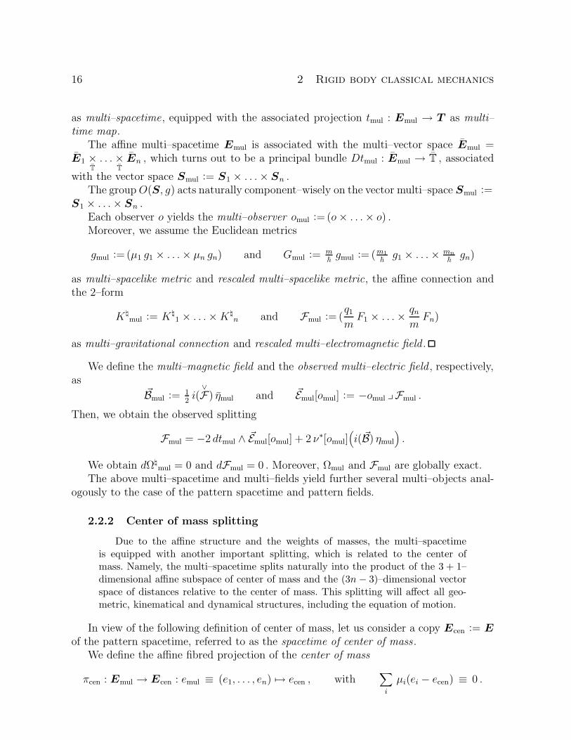
16 2 Rigid body classical mechanics
as multi–spacetime, equipped with the associated projection tmul : Emul → T as multi–
time map.The affine multi–spacetime Emul is associated with the multi–vector space Emul =
E1 ×T. . . ×
TEn , which turns out to be a principal bundle Dtmul : Emul → T , associated
with the vector space Smul := S1 × . . .× Sn .The groupO(S, g) acts naturally component–wisely on the vector multi–space Smul :=
S1 × . . .× Sn .Each observer o yields the multi–observer omul := (o× . . .× o) .Moreover, we assume the Euclidean metrics
gmul := (µ1 g1 × . . .× µn gn) and Gmul := m~gmul := (m1
~g1 × . . .× mn
~gn)
as multi–spacelike metric and rescaled multi–spacelike metric, the affine connection andthe 2–form
Kmul := K
1 × . . .×Kn and Fmul := (
q1mF1 × . . .×
qnmFn)
as multi–gravitational connection and rescaled multi–electromagnetic field .
We define the multi–magnetic field and the observed multi–electric field , respectively,as
~Bmul := 12i(
∨
F) ηmul and ~Emul[omul] := −omul yFmul .
Then, we obtain the observed splitting
Fmul = −2 dtmul ∧ ~Emul[omul] + 2 ν∗[omul](i( ~B) ηmul
).
We obtain dΩmul = 0 and dFmul = 0 . Moreover, Ωmul and Fmul are globally exact.
The above multi–spacetime and multi–fields yield further several multi–objects anal-ogously to the case of the pattern spacetime and pattern fields.
2.2.2 Center of mass splitting
Due to the affine structure and the weights of masses, the multi–spacetimeis equipped with another important splitting, which is related to the center ofmass. Namely, the multi–spacetime splits naturally into the product of the 3 + 1–dimensional affine subspace of center of mass and the (3n − 3)–dimensional vectorspace of distances relative to the center of mass. This splitting will affect all geo-metric, kinematical and dynamical structures, including the equation of motion.
In view of the following definition of center of mass, let us consider a copy Ecen := E
of the pattern spacetime, referred to as the spacetime of center of mass.We define the affine fibred projection of the center of mass
πcen : Emul → Ecen : emul ≡ (e1, . . . , en) 7→ ecen , with∑
i
µi(ei − ecen) ≡ 0 .

2.2 Multi-body mechanics 17
We can view the space of center of mass also in another way. In fact, let us considerthe 3–dimensional diagonal affine subspace idia : Edia → Emul . Clearly, the restrictionof πcen to Edia yields an affine fibred isomorphism Edia → Ecen . We shall often identifythese two spaces via the above isomorphism and write icen : Ecen → Emul .
Moreover, we define the center of mass space and the relative space to be, respectively,the 3–dimensional and the (3n− 3)–dimensional vector subspaces of Smul
Scen := vmul ∈ Smul | v1 = . . . vn , Srel := vmul ∈ Smul |∑
i
µi vi = 0 .
Of course, the natural action of O(S, g) on Smul restricts to a free action on Srel .
We set Erel := T × Srel .
Then, we obtain the affine fibred splitting over T
Emul → Edia ×T
Erel = Edia × Srel ≃ Ecen ×T
Erel = Ecen × Srel :
: emul 7→ (ecen, vrel) :=(πcen(emul), emul − idia(ecen)
).
We stress that the above splitting yields the natural projections Emul → Edia andEmul → Srel and the natural inclusion Edia → Emul , but it does not yield a naturalinclusion Srel → Emul .
The above splitting yields several other splittings.
2.1 Proposition. We have the following linear splittings of vector spaces
Emul → Ecen × Srel : (v1, . . . , vn) 7→( ∑
i
µi vi , (v1 −∑
i
µi vi , . . . , vn −∑
i
µi vi)).
E∗mul → E
∗cen × S∗
rel : (α1, . . . , αn) 7→( ∑
i
αi , (α1 − µ1 (∑
i
αi) , . . . , αn − µn (∑
i
αi))).
These splittings turn out to be affine fibred splittings over T orthogonal with respectto the rescaled metric Gmul .
The multi–metric gmul splits into the product of a metric gdia ≃ gcen of Edia ≃ Ecen
and a metric grel of Srel . We observe that gcen = g , in virtue of the equality∑
i µi = 1 .Therefore, the multi–metric Gmul splits into the product of the metric Gdia ≃ Gcen = m
~g
of Edia ≃ Ecen and the metric Grel = m~ grel of Erel .
The gravitational connectionKmul of the multi–spacetime Emul splits into the product
of a gravitational connection Kcen of Ecen and of a gravitational connection K
rel ofSrel . The connections K
cen and Krel coincide with the connections induced by the affine
structures of the corresponding spaces (because affine isomorphisms between affine spacespreserve the connections induced by the affine structures). Moreover, the connectionsK
cen and Krel preserve the metrics gcen and grel .

18 2 Rigid body classical mechanics
2.2.3 Multi–electromagnetic field
The splitting of the multi–spacetime yields a splitting of the multi–electromagneticfield.
2.2 Proposition. The isomorphism Ecen × Srel → Emul yields a splitting of Fmul
into the three components
Fmul = Fmul cen + Fmul rel + Fmul cen rel ,
where
Fmul cen : Emul → (L1/2 ⊗ M1/2) ⊗ Λ2T ∗Ecen ⊂ (L1/2 ⊗ M1/2) ⊗ Λ2T ∗Emul ,
Fmul rel : Emul → (L1/2 ⊗ M1/2) ⊗ Λ2T ∗Srel ⊂ (L1/2 ⊗ M1/2) ⊗ Λ2T ∗Emul ,
Fmul cen rel : Emul → (L1/2 ⊗ M1/2) ⊗ (T ∗Ecen ∧ T∗Srel) ⊂ (L1/2 ⊗ M1/2) ⊗ Λ2T ∗Emul ,
according to the following formula
Fmul cen(emul; vmul, wmul) =∑
i
qi
mFi(ei; vcen i, wcen i) ,
Fmul rel(emul; vmul, wmul) =∑
i
qi
mFi(ei; ~vrel i, ~wrel i) ,
Fmul cen rel(emul; vmul, wmul) =∑
i
qi
mFi(ei; vcen i, ~wrel i) +
∑
i
qi
mFi(ei; ~vrel i, wcen i) ,
i.e.
Fmul cen(emul; vmul, wmul) =
= −o(vcen)∑
i
qi
m~Ei[o](ei) · ~wcen[o] + o(wcen)
∑
i
qi
m~Ei[o](ei) · ~vcen[o]
+∑
i
qi
m~Bi(ei) · (~vcen[o] × ~wcen[o]) ,
Fmul rel(emul; vmul, wmul) =∑
i
qi
m~Bi(ei) · (~vrel i × ~wrel i)
Fmul cen rel(emul; vmul, wmul) =
= −o(vcen)∑
i
qi
m~Ei[o](ei) · ~wrel i +
∑
i
qi
m~Bi(ei) · (~wrel i × ~vcen[o]
)
+ o(wcen)∑
i
qi
m~Ei[o](ei) · ~vrel i −
∑
i
qi
m~Bi(ei) · (~vrel i × ~wcen[o]) .
for each emul ∈ Emul and vmul = vcen + ~vrel ∈ Emul = Ecen + Srel .
On the other hand, the inclusion icen : Ecen → Emul yields the scaled the 2–form
Fcen := i∗cenFmul = Fmul cen icen : Ecen → (L1/2 ⊗ M1/2) ⊗ Λ2T ∗Ecen ,

2.3 Rigid body mechanics 19
given by
Fcen(ecen; vcen, wcen) = qmF (ecen; vcen, wcen) .
If qi = kmi and F is spacelikely affine, then Fmul cen ≃ Fcen and Fmul cen rel = 0 .
2.3 Proposition. The potential Amul for Fmul splits as
Amul = Acen + Arel , where Acen : Emul → T ∗Ecen , Arel : Emul → T ∗Erel ,
with Acen(emul; vmul) =∑
iqi
mAi
(ei; vcen i
)and Arel(emul; vmul) =
∑i
qi
mAi
(ei; vrel i
).
We stress that, in general, each of the three components of the multi–electromagneticfield depends on the whole multi–spacetime and not just on the corresponding compo-nents. Hence, in general, the joined multi–connection Kmul does not split into the productof a joined multi–connection Kcen of Ecen and of a multi–connection Krel of Erel . As aconsequence, in general, the equation of motion of the multi–particle splits into a systemof equations for the motion of the center of mass and for the relative multi–motion, whichare coupled.
However, in the particular case when the pattern electromagnetic field F is constantand the charges are proportional to the masses (i.e., qi = kmi) the mixed term Fcen rel
vanishes. In this case, the rescaled multi–electromagnetic field Fmul splits truly with re-spect to the two components of the multi–spacetime Ecen and Srel . Therefore, also thejoined multi–connection splits with respect to Ecen and Srel . Hence, the equation of mo-tion of the multi–particle splits into a decoupled system of equations for the motion ofthe center of mass and for the relative multi–motion.
2.3 Rigid body mechanics
Finally, we achieve the scheme for a rigid body in the framework of “covari-ant classical mechanics”, by considering a space-like rigid constraint on the multi–spacetime and assuming as spacetime for the rigid body the constrained subbundleof the multi–spacetime, which is called rigid body spacetime. All objects relatedto this rigid–spacetime are called rigid–body objects and labelled by the subscript“rig” .
2.3.1 Configuration space
To carry on our analysis, we need a ‘generalised’ definition of affine space. Namely,we define a generalised affine space to be a triple (A,G, ·) , where A is a set, G a groupand · a transitive and free left action of G on A . Note that, for every a ∈ A , the ‘lefttranslation’ L(a) : G→ A : g 7→ ga is a bijection.
The generalised affine space A is naturally parallelisable as TA = A × g , where g isthe Lie algebra of G .
We consider a set lij ∈ L2 | i, j = 1, . . . , n, i 6= j, lij = lji, lik ≤ lij + ljk and

20 2 Rigid body classical mechanics
define the subsets
irig : Erig := emul ∈ Emul | ‖ei − ej‖ = lij , 1 ≤ i < j ≤ n → Emul ,
irot : Srot := vrel ∈ Srel | ‖vi − vj‖ = lij , 1 ≤ i < j ≤ n → Srel .
We set Erot := T × Srot .We stress that the rigid constraint does not affect the center of mass.The inclusion irig turns out to be equivariant with respect to the left action of
O(S, g) , because the rigid constraint is invariant with respect to this group.Then, the spacelike orthogonal affine splitting Emul = Ecen ×
TErel = Ecen × Srel
restricts to a splitting
Erig = Ecen ×T
Erot = Ecen × Srot .
Thus, we obtain a curved fibred manifold trig : Erig → T consisting of the fibredproduct over T of the affine bundles tcen : Ecen → T and trot : Erot → T , or, equivalently,consisting of the Cartesian product of the affine bundle tcen : Ecen → T with the spacelikesubmanifold Srot ⊂ Srel .
The 1st jet space of Erig splits as J1Erig ≃ (Ecen × U cen) × (T∗ ⊗ TSrot) .Each rigid observer o : E → J1E , induces an observer orig : Erig → J1Erig . In
particular, each inertial observer o ∈ U induces an observer orig ∈ U cen , which is stillcalled inertial .
The inclusion irig yields the scaled spacelike Riemannian metric
grig := i∗rig gmul : TErig ×Erig
TErig → L2 ⊗ IR .
In order to further analyse the geometry of Erig , it suffices to study Srot .
2.3.2 Rotational space
The geometry of Srot depends on the initial mutual positions of particles and is timeindependent. In particular, particles can either lie on a straight line, or lie on a plane, or“span” the whole space. This can be formalised as follows.
For each rrot ∈ Srot , let us consider the vector space
〈rrot〉 := span(ri − rj) | 1 ≤ i < j ≤ n
⊂ S .
We can prove that the dimension of this space depends only on Srot and not on thechoice of rrot ∈ Srig . We call this invariant number crot the characteristic of Srot . We canhave crot = 1, 2, 3 . We say that Srot is strongly non degenerate if crot = 3 , weakly non
degenerate if crot = 2 , degenerate if crot = 1 .We observe that the natural actions of O(S, g) on Srel restricts to Srot .

2.3 Rigid body mechanics 21
The inclusion irot turns out to be equivariant with respect to the left action of O(S, g) ,because the rigid constraint is invariant with respect to this group.
The action of O(S, g) on Srot is transitive.For each vrot ∈ Srot , let us call H [rrot] ⊂ O(S, g) the corresponding isotropy subgroup.We can see that:- in the strongly non degenerate case the isotropy subgroup H [rrot] is the trivial sub-
group 1 ;- in the weakly non degenerate case the isotropy subgroup H [rrot] is the discrete sub-
group of reflections with respect to 〈vrot〉 ;- in the degenerate case the isotropy subgroup H [rrot] is the 1 dimensional subgroup
of rotations whose axis is 〈rrot〉 ; we stress that this subgroup is not normal.Hence, we can prove that:– Srot is strongly non degenerate if and only if the action of O(S, g) on Srot is free;– Srot is weakly non degenerate if and only if the action of O(S, g) on Srot is not free,
but the action of SO(S, g) on Srot is free;– Srot is degenerate if and only if the action of SO(S, g) on Srot is not free.Of course, if n = 2 , then Srot is degenerate; if n = 3 , then Srot can be degenerate or
weakly non degenerate.Furthermore, we can prove that:– if Srot is strongly non degenerate, then Srot is an affine space associated with the
group O(S, g) ;– if Srot is weakly non degenerate, then Srot is an affine space associated with the
group SO(S, g) ;– if Srot is degenerate, then Srot is a homogeneous manifold with two possible distin-
guished diffeomorphisms (depending on a chosen orientation on the straight line of therigid body) with the unit sphere S2(L∗ ⊗ S, g) .
So, the choice of a configuration vrot ∈ Srot and of a scaled orthonormal basis in S ,respectively, yields the following diffeomorphisms (via the action of O(S, g) on Srot)
Srot ≃ O(S, g) ≃ O(3) , in the strongly non degenerate case;
Srot ≃ SO(S, g) ≃ SO(3) , in the weakly non degenerate case;
Srot ≃ S2 ≃ S2 , in the degenerate case,
where S2 ⊂ L∗ ⊗ S is the unit sphere with respect to the metric g .
From now on, for the sake of simplicity and for physical reasons of continuity, inthe non degenerate case, we shall refer only to one of the two connected components ofSrot . Accordingly, we shall just refer to the non degenerate case (without specification ofstrongly or weakly non degenerate) as to the degenerate cases.
2.4 Proposition. In the non degenerate case, by considering the isomorphism Srot ≃SO(3) , and the well known two–fold universal covering S3 ≃ SU(2) → SO(3) , we obtainthe universal covering S3 → Srot , which is a principal bundle associated with the groupZ2 [38, vol.1].
22 2 Rigid body classical mechanics
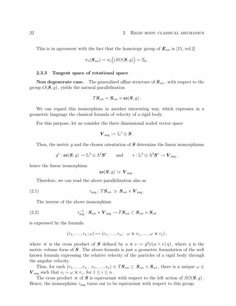
This is in agreement with the fact that the homotopy group of Erot is [15, vol.2]
π1(Srot) = π1
((SO(S, g)
)= Z2 .
2.3.3 Tangent space of rotational space
Non degenerate case. The generalised affine structure of Srot , with respect to thegroup O(S, g) , yields the natural parallelisation
TSrot = Srot × so(S, g) .
We can regard this isomorphism in another interesting way, which expresses in ageometric language the classical formula of velocity of a rigid body.
For this purpose, let us consider the three dimensional scaled vector space
V ang := L∗ ⊗ S .
Then, the metric g and the chosen orientation of S determine the linear isomorphisms
g : so(S, g) → L2 ⊗ Λ2S∗ and ∗ : L2 ⊗ Λ2S∗ → V ang ,
hence the linear isomorphism
so(S, g) ≃ V ang .
Therefore, we can read the above parallelization also as
(2.1) τang : TSrot ≃ Srot × V ang .
The inverse of the above isomorphism
(2.2) τ−1ang : Srot × V ang → TSrot ⊂ Srot × Srel
is expressed by the formula
(r1, . . . , rn ;ω) 7→ (r1, . . . , rn ; ω × r1, . . . , ω × r1) ,
where × is the cross product of S defined by u × v := g♯(i(u ∧ v) η) , where η is themetric volume form of S . The above formula is just a geometric formulation of the wellknown formula expressing the relative velocity of the particles of a rigid body throughthe angular velocity.
Thus, for each (r1, . . . , rn , v1, . . . , vn) ∈ TSrot ⊂ Srot × Srel , there is a unique ω ∈V ang such that vi = ω × ri , for 1 ≤ i ≤ n .
The cross product × of S is equivariant with respect to the left action of SO(S, g) .Hence, the isomorphism τang turns out to be equivariant with respect to this group.

2.3 Rigid body mechanics 23
The angular velocity of a rigid motion s : T → Erig is defined to be the map
ω := τang Tπrot ds : T → T∗ ⊗ V ang ,
where πrot : Erig → Srot is the natural projection map according to section 2.3.1.
We stress that the above geometric constructions use implicitly the pattern affinestructure. Hence, the angular velocity is independent of the choice of inertial observers.But, the observed angular velocity would depend on the choice of non inertial observers.
Degenerate case. According to a well–known result on homogeneous spaces, thetangent space of Srot turns out to be the quotient vector bundle
TSrot = Srot × so(S, g)/h[Srot] ,
where h[Srot] ⊂ Srot×so(S, g) is the vector subbundle over Srot consisting of the isotropyLie algebras of Srot .
Now, let us consider again the scaled vector space V ang := L∗ ⊗ S and define thequotient vector bundle over Srot
(Srot × V ang)/ ∼ ,
induced, for each rrot ∈ Srot , by the vector subspace 〈rrot〉 ⊂ V ang generated by rrot .
Then, by proceeding as in the non degenerate case and taking the quotient with respectto the isotropy subbundle, we obtain the linear fibred isomorphism
[τang] : TSrot ≃ (Srot × V ang)/ ∼ .
The inverse of the above isomorphism
[τang]−1 : (Srot × V ang)/ ∼ → TSrot ⊂ Srot × Smul
is expressed by the formula
(r1, . . . , rn ; [ω]) 7→ (r1, . . . , rn ; ω × r1, . . . , ω × r1) ,
where the cross products ω×ri turns out to be independent on the choice of representativefor the class [ω] .
Thus, for each (r1, . . . , rn , v1, . . . , vn) ∈ TSrot ⊂ Srot × Srel , there is a unique [ω] ∈(Srot × V ang)/ ∼|(r1,...,rn) such that vi = ω × ri , for 1 ≤ i ≤ n .
Clearly, each choice of the orientation of the rigid body yields a distinguished fibredisomorphism
TSrot ≃ TS2(L∗ ⊗ S, g) .

24 2 Rigid body classical mechanics
2.3.4 Induced metrics
The multi–metric of Smul induces a metric on Srot , which can be regarded alsoin another useful way through the isomorphism τang .
Even more, the standard pattern metric of V ang induces a further metric onSrot , which will be interpreted as the inertia tensor.
The inclusion irot yields the scaled Riemannian metric
grot := i∗rot grel : TSrot ×Srot
TSrot → L2 ⊗ IR .
We can regard this metric in another interesting way, which follows from the paral-lelisation through V ang .
For this purpose, the patter metric g can be regarded as a Euclidean metric of S
g : V ang × V ang → IR .
We can make the natural identifications O(V ang, g) ≃ O(S, g) .
Therefore, the isomorphism τang allows us to read grot as the scaled fibred Riemman-nian metric
σ := τ−1∗ang grot : Srot × (V ang × V ang) → L2 ⊗ IR
σ := τ−1∗ang grot :
(Srot × V ang)/ ∼
)×
Srot
(Srot × V ang)/ ∼
)→ L2 ⊗ IR ,
respectively, in the non degenerate and in the degenerate cases. Its expression is
σ(r1, . . . , rn ; ω, ω′) =∑
i
µi
(g(ri, ri) g(ω, ω
′) − g(ri, ω) g(ri, ω′)
)(2.3)
σ(r1, . . . , rn ; [ω], [ω′]) =∑
i
µi
(g(ri, ri) g(ω, ω
′) − g(ri, ω) g(ri, ω′)
),
respectively, in the non degenerate and in the degenerate cases.In the degenerate case, the above expression can be also written as
σ(r1, . . . , rn ; [ω], [ω′]) = g(ω, ω′)∑
i
µi g(ri, ri) ,
where ω and ω′ are the representatives of [ω] and [ω′] orthogonal to the ri’s .
Then, we obtain a further metric. In fact, the metric g of V ang can be regarded as afibred metric over Srot , which will be denoted by the same symbol,
g : Srot × (V ang × V ang) → IR
g :(Srot × V ang)/ ∼
)×
Srot
(Srot × V ang)/ ∼
)→ IR ,
2.3 Rigid body mechanics 25
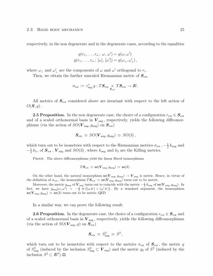
respectively, in the non degenerate and in the degenerate cases, according to the equalities
g(r1, . . . , rn ; ω, ω′) = g(ω, ω′)
g(r1, . . . , rn ; [ω], [ω′]) = g(ω⊥, ω′⊥) ,
where ω⊥ and ω′⊥ are the components of ω and ω′ orthogonal to ri .
Then, we obtain the further unscaled Riemannian metric of Srot
σrot := τ ∗ang g : TSrot ×Srot
TSrot → IR .
All metrics of Srot considered above are invariant with respect to the left action ofO(S, g) .
2.5 Proposition. In the non degenerate case, the choice of a configuration rrot ∈ Srot
and of a scaled orthonormal basis in V ang , respectively, yields the following diffeomor-phisms (via the action of SO(V ang, gang) on Srot)
Srot ≃ SO(V ang, gang) ≃ SO(3) ,
which turn out to be isometries with respect to the Riemannian metrics σrot , −12kang and
−12k3 , of Srot , V ang and SO(3) , where kang and k3 are the Killing metrics.
Proof. The above diffeomorphisms yield the linear fibred isomorphisms
TSrot ≃ so(V ang, gang) ≃ so(3) .
On the other hand, the natural isomorphism so(V ang, gang) → V ang is metric. Hence, in virtue ofthe definition of σrot , the isomorphism TSrot ≃ so(V ang, gang) turns out to be metric.
Moreover, the metric gang of V ang turns out to coincide with the metric − 12
kang of so(V ang, gang) . Infact, we have gang(ω, ω′) = − 1
2tr
((ω×) (ω′
×)). By a standard argument, the isomorphism
so(V ang, gang) ≃ so(3) turns out to be metric. QED
In a similar way, we can prove the following result.
2.6 Proposition. In the degenerate case, the choice of a configuration rrot ∈ Srot andof a scaled orthonormal basis in V ang , respectively, yields the following diffeomorphisms(via the action of SO(V ang, g) on Srot)
Srot ≃ S2ang ≃ S2 ,
which turn out to be isometries with respect to the metrics σrot of Srot , the metric gof S2
ang (induced by the inclusion S2ang ⊂ V ang) and the metric g2 of S2 (induced by the
inclusion S2 ⊂ IR3).

26 2 Rigid body classical mechanics
Inertia tensor. The fibred metric g of Srot allows us to regard the fibred metric σof Srot as a scaled symmetric fibred automorphism
σ : Srot → L2 ⊗ (V ∗ang × V ang) .
The scaled metric mσ , or the scaled automorphism mσ , are called the inertia tensor .The scaled eigenvalues of the inertia tensor are called principal inertia momenta and aredenoted by Ii ∈ map(Srot, L2 ⊗M⊗ IR) . Indeed, the principal inertia momenta turn outto be constant with respect to Srot .
In the non degenerate case, we have three principal inertia momenta. Then, threecases can occur:
I := I1 = I2 = I3 , spherical case ,
I := I1 = I2 6= I3 , symmetric case ,
I1 6= I2 6= I3 6= I1 , asymmetric case.
In the degenerate case, we have two coinciding principal inertia momenta
I := I1 = I2 =∑
i
mi g(ri, ri) .
In the spherical non degenerate case and in the degenerate case, we have
(2.4) grot =I
mσ .
Thus, we have studied the diagonalisation of σ with respect to g . In an analogousway, we can diagonalise grot with respect to σrot . Indeed, in this way we obtain the sameeigenvalues and the same classification, because the two diagonalisations are related bythe isomorphism τang .
The principal inertia momenta are related to the scalar curvature of the rotationalspace in the following way.
2.7 Proposition. The scalar curvature of Srot , with respect to the metric Grot , is[58]
ρrot =3 ~
2 I, sph. non deg. case, with I := I1 = I2 = I3 ,
ρrot =2 ~
I1−
~ I
2 I21
, sym. non deg. case, with I := I2 = I3 ,
ρrot =~
I1+
~
I2+
~
I3−
~ (I21 + I2
2 + I23 )
2 I1 I2 I3, asym. non deg. case,
ρrot =2 ~
I, deg. case, with I := I1 = I2 .

2.3 Rigid body mechanics 27
Moreover, since the splitting Erig = Ecen × Srot is orthogonal, the vanishing of thescalar curvature ρ yields ρrig = ρrot .
2.3.5 Induced connection
The multi–connection of the multi–spacetime induces naturally a connection onthe rigid configuration space, which splits naturally into the center of mass andrelative components.
We can easily state the following generalisation of a well known theorem due to Gauss[38].
2.8 Lemma. Let us consider a fibred manifold p : F → B equipped with a verticalRiemannian metric gF and a linear connection KF of F , which restricts to the fibres ofF → B and preserves the metric gF .
Moreover, let us consider a fibred submanifold G ⊂ F over B and the orthogonalprojection πG : TF |G → TG induced by gF .
Then, there exists a unique linear connection KG of G , which restricts to the fibres ofG → B and such that, for every pair of vector fields X, Y of G , we have πG(∇[KF ]XY ) =∇[KG]XY . Moreover, this connection KG preserves gG .
According to the above Lemma, the connectionKmul of Emul yields a linear connection
Krig of Erig , which preserves the time fibring and the metric grig .
Moreover, according to a standard result due to Gauss, the connection Krel of Srel
induces a connection κrot on Srot , which coincides with the Riemannian connection
induced by grot .
2.9 Proposition. By considering the splitting Erig = Ecen × Srot , the connectionK
rig splits into the product of the connections Kcen and κ
rot .
Proof. We have the splitting Kmul = K
cen × Krel . Moreover, the splitting Emul = Ecen × Srel
is orthogonal with respect to the metric gmul , hence the projection πErigsplits into the projections
Emul → Ecen and Emul → Srel .
Hence, Krig splits into the product of the connections K
cen and κrot . QED
2.3.6 Induced electromagnetic field
We analyse the pullback of the multi electromagnetic field on the rigid space-time. This is a 2–form on a 1+6 dimensional manifold in the non degenerate caseand on a 1+5 dimensional manifold in the degenerate case. We can express this2–form in terms of the pattern electric and magnetic fields.
We can decompose this form into three components: the center of mass compo-nent, the rotational component and the mixed component. In the particular casewhen the mixed component vanishes and the other two components depend onlyon the center of mass and rotational variables, these two components coincide with

28 2 Rigid body classical mechanics
the pullback of the multi electromagnetic field with respect to the center of massand rotational projections.
Indeed, we can prove that the pullback of the multi–electromagnetic field onthe rigid spacetime provides the suitable electromagnetic object for the correct ex-pression of the classical law of motion (in the context of our formulation of classicalmechanics of a rigid body interpreted as a classical particle moving in a higherdimensional spacetime).
Therefore, we shall assume this pullback also as the correct object for our for-mulation of quantum mechanics of a rigid body.
Non degenerate case. Let us start by studying the non degenerate case.
2.10 Proposition. The inclusion irig : Erig = Ecen × Srot → Emul yields the scaled2–form
Frig := i∗rigFmul ,
which splits into the three components
Frig = Frig cen + Frig rot + Frig cen rot ,
where
Frig cen : Erig → (L1/2 ⊗ M1/2) ⊗ Λ2T ∗Ecen
Frig rot : Erig → (L1/2 ⊗ M1/2) ⊗ Λ2T ∗Srot
Frig cen rot : Erig → (L1/2 ⊗ M1/2) ⊗ (T ∗Ecen ∧ T∗Srot) ,
according to the following formula
Frig cen(erig; vrig, wrig) =∑
i
qi
mFi
(ei; vcen i, wcen i
)
Frig rot(erig; vrig, wrig) =∑
i
qi
mFi
(ei; ω × ri, ψ × ri
)
Frig cen rot(erig; vrig, wrig) =∑
i
qi
mFi
(ei; vcen i, ψ × ri
)+
∑
i
qi
mFi
(ei; ω × ri, wcen i
),
for each
(erig, vrig) = (ecen, r1, . . . , rn ; vcen + ω × r1 + · · ·+ ω × rn) ∈ TErig ,
(erig, wrig) = (ecen, r1, . . . , rn ; wcen + ψ × r1 + · · · + ψ × rn) ∈ TErig ,

2.3 Rigid body mechanics 29
i.e.
Frig cen(erig; vrig, wrig) =∑
i
qi
m~Ei[o](ei) · (~vcen[o] − ~wcen[o])
+∑
i
qi
m~Bi(ei) ·
(~vcen[o] × ~wcen[o]
)
Frig rot(erig; vrig, wrig) =∑
i
qi
m
(~Bi(ei) · ri
) ((ω × ψ) · ri
)
Frig cen rot(erig; vrig, wrig) =∑
i
qi
m~Ei[o](ei) ·
((ω − ψ) × ri
)
+∑
i
qi
m
(~Bi(ei) · ψ
) (~vcen[o] · ri
)
−∑
i
qi
m
(~Bi(ei) · rrot i
) (~vcen[o] · ψ
)
−∑
i
qi
m
(~Bi(ei) · ω
) (~wcen[o] · rrot i
)
+∑
i
qi
m
(~Bi(ei
)· rrot i
) (~wcen[o] · ω
).
If qi = kmi and F is spacelikely affine, then Frig cen ≃ Fcen and Frig cen rot = 0 .
2.11 Proposition. The potential Arig := i∗rigAmul for Frig splits as
Arig = Arig cen + Arig rot , where Arig cen : Erig → T ∗Ecen , Arig rot : Erig → T ∗S∗ ,
with Acen(erig; vrig) =∑
iqi
mAi(erig i; vcen i) and Arel(erig; vrig) =
∑i
qi
mAi(erig i; vrot i) .
Degenerate case. The degenerate case can be studied in a similar way to the nondegenerate one.
Here, we just provide, as an example, an explicit description of a dipole, consisting of2 particles with opposite charges in a constant electromagnetic field. In this case, we have
Frig cen(e1, e2; vrig, wrig) =∑
i
qi
mF (vcen, wcen) = 0
Frig rot(e1, e2; vrig, wrig) = q1
mF (vrot 1, wrot 1) −
q1
m(m1
m2)2F (vrot 1, wrot 1)
= q1m2−m1
m22
F (vrot 1, wrot 1)
= 2 q1m2−m1
m22
~B · (vrot 1 × wrot 1)
Frig cen rot(e1, e2; vrig, wrig) = q1
mF (vcen 1, wrot 1) −
q1
mF (vcen 2, wrot 2)
+ q1
mF (vrot 1, wcen 1) −
q1
mF (vrot 2, wcen 2)
= q1
mF (vcen 1, wrot 1) + m1
m2
q1
mF (vcen 1, wrot 1)
+ q1
mF (vrot 1, wcen 1
)+ m1
m2
q1
mF (vrot 1, wcen 1)

30 2 Rigid body classical mechanics
= 2 q1
m2
~E[o] · (w0cen vrot 1) − v0
cen wrot 1))
+ 2 ~B · g(vrot 1 × ~wcen[o] + wrot 1 × ~vcen[o]) .
2.3.7 Spacetime structures
The previous results suggest a model for the classical mechanics of a rigid bodycompletely analogous to our one–body scheme.
We assume the fibred manifold trig : Erig → T as rigid–body spacetime. Moreover,we assume the metric grig := i∗rig gmul as the spacelike metric, the metric Grig = m
~grig as
the rescaled spacelike metric, the connection Krig = K
cen × κrig as the gravitational
connection, the 2–form Frig := i∗rig Fmul as the rescaled electromagnetic field , and the 2–form m
~Frig as the unscaled electromagnetic field .
The joined cosymplectic 2–form Ωrig induced by the above gravitational connection,the unscaled electromagnetic field and the rescaled metric coincides with the pullbackΩrig = i∗Ωmul .
Hence, Ωrig turns out to be a globally exact cosymplectic 2–form.
The velocity space of Erig splits as
J1Erig ≃ (Ecen × U cen) × (T∗ ⊗ TSrot) .
An inertial observer o yields the further splitting Ecen = T × P [o]cen .Given an inertial observer o , we shall refer to a spacetime chart (x0, xi, xα) adapted
to the observer and to the center of mass splitting. Here, indices i, j will label coordinatesof P [o]cen and α, β will label coordinates of Srot (e.g., Euler angles).
2.3.8 Dynamical functions
Here, we discuss the momentum and Hamiltonian functions and their splittinginto the translational and rotational components.
Let us choose a horizontal potential A↑rig for Ωrig and an inertial observer o .
They yield the rigid momentum and Hamiltonian
Prig := ν[o] yA↑rig : J1Erig → T ∗Erig , Hrig := −o yA↑
rig : J1Erig → T ∗Erig ,
which split asPrig = Pcen + Prot , Hrig = Hcen + Hrot ,
where
Pcen : J1Erig → T ∗Ecen , Prot : J1Erig → T ∗Erot ,
Hcen : J1Erig → T ∗Ecen , Hcen : J1Erig → T ∗Erot .

2.3 Rigid body mechanics 31
We have the coordinate expressions
Pcen j = Gcen0ij x
j0 + Acen i , Prot α = Grot
0αβ x
β0 + Arot α ,
Hcen 0 = 12Gcen
0ij x
i0 x
j0 −Acen 0 , Hrot 0 = 1
2Grot
0αβ x
α0 x
β0 − Arot 0 .
Clearly, Pcen and Prot can be identified with the angular momentum of the center ofmass and the angular momentum with respect to the center of mass, respectively.
In the general case they are coupled and not conserved.In the particular case when F = 0 , they are conserved and we obtain the decoupled
expressions
Pcen : J1Ecen → T ∗Ecen , Prot : J1Erot → T ∗Erot ,
Hcen : J1Ecen → T ∗Ecen , Hcen : J1Erot → T ∗Erot .

32 3 Rigid body quantum mechanics
3 Rigid body quantum mechanics
In the previous chapter we have described the classical framework of a rigidbody in analogy with the framework of a constrained one–body. Then, we approachthe quantisation of the rigid body according to the scheme of “covariant quantummechanics”, by analogy with the case of a one-body.
We define quantum structures, analyse their existence and classify them. Then,we evaluate the quantum operators and compute the spectra of the energy operatorin some cases.
3.1 Quantum structures
First, we analyse the existence and classification of quantum structures according toProposition 1.1.
The existence condition of the quantum structure is fulfilled due to the exactness ofΩrig :
[Ω] = 0 ∈ i2(H2(E,Z)
)⊂ H2(E, IR) ≃ H2(J1E, IR) .
So, we have just to compute all possible inequivalent quantum structures.
Non degenerate case. Let us start with the non degenerate case.
3.1 Proposition. We have just two equivalence classes of complex line bundles overErig . Clearly, one of these classes is the trivial one. Indeed, both of them admit quantumconnections.
Proof. The 2nd cohomology groups of Erig are [6]:
H2(Erig, Z) ≃ H2(Srig, Z) ≃ H2(SO(S, g), Z
)≃ Z2 ,
H2(Erig, IR) ≃ H2(Srig, IR) ≃ H2(SO(S, g), IR
)≃ 0 .
Then, according to Proposition 1.1, the equivalence classes of complex line bundles are in bijectionwith H2(Erig, Z) = Z2 and the equivalence classes of quantum bundles are in bijection with (i2)−1([Ω]) =(i2)−1(0) = Z2 . QED
We can produce two concrete representatives for the above equivalence classes of vectorbundles in the following way.
3.2 Lemma. The two inequivalent representations of Z2 on C yield the trivial Her-mitian line bundle Q+
rot and the non trivial Hermitian line bundle Q−rot , equipped with
flat Hermitian connections χ+rot and χ−
rot , respectively.These bundles admit an atlas with constant transition maps and the above flat con-
nections have vanishing symbols with respect to this atlas.
Proof. Let us consider the two inequivalent representations of Z2 on C
ρ+(1) = 1 , ρ+(−1) = 1 and ρ−(1) = 1 , ρ−(−1) = −1 .

3.1 Quantum structures 33
Then, the quotient of the trivial Hermitian line bundle Qrot = S3 × C → S3 with respect to theabove actions of Z2 yields, respectively, the associated trivial and non trivial Hermitian line bundles overSrot
Q+rot = S3 ×
ρ+
C and Q−rot = S3 ×
ρ−
C .
Moreover, the natural flat principal connection of the principal bundle S3 → SO(3) yields two flatHermitian connections χ+
rot and χ−rot on Q+
rot and Q−rot , respectively.QED
3.3 Proposition. The pullback with respect to the projection Erig → Srot yields atrivial and a non trivial Hermitian line bundle
Q+rig → Erig and Q−
rig → Erig ,
which are equipped with the pullback flat Hermitian connections χ+rig and χ−
rig , respec-tively.
3.4 Theorem. Let Erig be non degenerate. Then, the only inequivalent quantum
structures are of the type (Q+rig,Q
↑+rig) and (Q↑−
rig,Q↑−rig) , with
Q↑+rig = χ↑+
rig + iA↑+rig ⊗ I↑ and Q
↑−rig = χ↑−
rig + iA↑−rig ⊗ I↑ ,
where χ↑+rig , χ
↑−rig are the pullbacks of χ+
rig , χ−rig , and A↑+
rig , A↑−rig are two global horizontal
potentials for Ω .
Proof. According to Proposition 1.1, inequivalent quantum structures are in bijection with the set
(i2)−1([Ωrig]) × H1(Erig, IR)/H1(Erig, Z) = Z2 × 0 .
More precisely, the 1st factor parametrises admissible quantum bundles and the 2nd factor paramet-rises quantum connections.QED
In the following, we will specify the two possible trivial and non trivial cases by thesuperscripts + or − only when it is required by the context.
Degenerate case. Next, we analyse the degenerate case, following the same linesof the non degenerate case.
3.5 Proposition. We have countably many equivalence classes of complex line bun-dles with basis Erig and just one equivalence class of quantum bundles. Namely, this isthe trivial one.
Proof. The 2nd cohomology group of Erig is
H2(Erig, Z) ≃ H2(Srig, Z) ≃ H2(S2, Z
)≃ Z
H2(Erig, IR) ≃ H2(Srig, IR) ≃ H2(S2, IR
)≃ IR .
Then, according to Proposition 1.1, the equivalence classes of complex vector bundles are in bijectionwith H2(Erig, Z) ≃ Z and the equivalence classes of quantum bundles are in bijection with (i2)−1([Ω]) =(i2)−1(0) = 0 .QED

34 3 Rigid body quantum mechanics
3.6 Theorem. Let Erig be degenerate. Then, the only quantum structure is of the
type (Qrig,Q↑rig) , with
Q↑rig = χ↑
rig + iA↑rig ⊗ I↑ ,
where χ↑rig is the pullback of χrig and A↑
rig is a global horizontal potential for Ωrig .
Proof. According to Proposition 1.1, inequivalent quantum structures are in bijection with the set
(i2)−1([Ωrig]) × H1(Erig, IR)/H1(Erig, Z) = 0 × 0 .
More precisely, the 1st factor parametrises admissible quantum bundles and the 2nd factor paramet-rises quantum connections.QED
Distinguished representatives. In both non degenerate and degenerate cases, thefollowing facts hold.
3.7 Proposition. Let us consider a global observer o : Erig → J1Erig .The form −Krig[o] + Qrig[o] turns out to be a global horizontal potential for Ω .Then, in the particular case when F = 0 , we can choose a representative of the
quantum structure (Qrig, Q↑rig) in each equivalence class, such that Arig[o] = 0 .
Hence, the quantum differential turns out to be just the covariant differential ∇[χrig]associated with the flat connection(s) χrig and the observed quantum Laplacian turns outto be just the (spacelike) scaled Bochner Laplacian ∆[χrig, grig] of the quantum bundleinduced by the flat connection(s) χrig and the (spacelike) metric grig .
3.8 Proposition. The Hermitian quantum bundle can be written, up to an equiva-lence, as the fibred complex tensor product over T
Qrig = Qcen ⊗T
Qrot ,
where Qcen → Ecen is a Hermitian (trivial) quantum bundle over Ecen and Qrot → Erot
is a Hermitian quantum bundle over Erot .
Accordingly, each quantum section Ψrig can be written as a finite sum of tensor prod-ucts of the type Ψcen ⊗ Ψrot , which represent quantum states with decoupled center ofmass and rotational modes.
3.2 Quantum dynamics
Now, we apply the machinery of “covariant quantum mechanics” to each one ofthe above three possible choices of quantum structures.
We will not repeat the whole procedure, but only sketch the main differencesbetween the one–body case and the rigid body case. As one can expect, the mostremarkable facts are due to the splitting Erig = Ecen × Srot .
The approach will be formally similar in the three cases, but the equations willprovide different results, as we will see in the next section.
3.2 Quantum dynamics 35
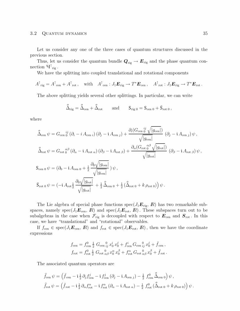
Let us consider any one of the three cases of quantum structures discussed in theprevious section.
Thus, let us consider the quantum bundle Qrig → Erig and the phase quantum con-nection Q↑
rig .
We have the splitting into coupled translational and rotational components
A↑rig = A↑
cen + A↑rot , with A↑
cen : J1Erig → T ∗Ecen , A↑rot : J1Erig → T ∗Erot .
The above splitting yields several other splittings. In particular, we can write
o
∆rig =o
∆cen +o
∆rot and Srig 0 = Scen 0 + Srot 0 ,
where
o
∆cen ψ = Gcenij0 (∂i − i Acen i) (∂j − iAcen j) +
∂i(Gcenij0
√|gcen|)√
|gcen|(∂j − iAcen j)ψ ,
o
∆rot ψ = Grotαβ0 (∂α − iArot α) (∂β − iArot β) +
∂α(Grotαβ0
√|grot|)√
|grot|(∂β − iArot β)ψ ,
Scen 0 ψ = (∂0 − iAcen 0 + 12
∂0
√|gcen|√|gcen|
)ψ ,
Srot 0 ψ = (−iArot12
∂0
√|grot|√|grot|
+ 12
o
∆cen 0 + 12(
o
∆rot 0 + k ρrot 0))ψ .
The Lie algebra of special phase functions spec(J1Erig, IR) has two remarkable sub-spaces, namely spec(J1Ecen, IR) and spec(J1Erot, IR) . These subspaces turn out to besubalgebras in the case when Frig is decoupled with respect to Ecen and Srot . In thiscase, we have “translational” and “rotational” observables.
If fcen ∈ spec(J1Ecen, IR) and frot ∈ spec(J1Erot, IR) , then we have the coordinateexpressions
fcen = f 0cen
12Gcen
0ij x
i0 x
j0 + f i
cen Gcen0ij x
j0 + f cen ,
frot = f 0rot
12Grot
0αβ x
α0 x
β0 + fα
rotGrot0αβ x
β0 + f rot .
The associated quantum operators are
fcen ψ =(f cen − i 1
2∂jf
jcen − i f j
cen (∂j − iAcen j) −12f 0
cen
o
∆cen 0
)ψ ,
frot ψ =(f rot − i 1
2∂αf
αrot − i fα
rot (∂α − iArot α) − 12f 0
rot (o
∆rot 0 + k ρrot 0))ψ .

36 3 Rigid body quantum mechanics
In particular, we have the following special phase functions
x0, xicen ∈ spec(J1Ecen, IR) , x0, xα
rot ∈ spec(J1Erot, IR) ,
Pcen j , ‖Pcen‖2 ∈ spec(J1Ecen, IR) , Prot α , ‖Prot‖
2 ∈ spec(J1Erot , IR) ,
Hcen 0 ∈ spec(J1Ecen, IR) , Hrot 0 ∈ spec(J1Erot, IR) .
and the associated quantum operators
xicen ψ = xi ψ , Pcen j ψ = −i (∂j + 1
2
∂j
√|gcen|√|gcen|
)ψ ,
Hcen 0 ψ =(− 1
2
o
∆cen 0 − Acen 0
)ψ ,
xαrot ψ = xα
rot ψ , Prot α ψ = −i (∂α + 12
∂α
√|grot|√
|grot|)ψ ,
Hrot 0 ψ =(− 1
2
o
∆rot 0 + k ρrot 0 − Arot 0
)ψ ,
and
‖Pcen‖20 ψ =
(Gij
cen 0Acen iAcen j − i(∂hA
hcen + 2Ah
cen (∂h − iAcen h))−
o
∆cen 0
)ψ
‖Prot‖20 ψ =
(Gαβ
rot 0Arot αArot β − i(∂αA
αrot + 2Aα
rot (∂α − iArot α))−
o
∆rot 0 − k ρrot 0
)ψ .

37
4 Rotational quantum spectra
4.1 Angular momentum in the free case
In this section, we analyse the implementation of angular momentum for a rigidbody in the framework of covariant quantum mechanics. We start by recalling therelevant facts concerning angular momentum in covariant classical mechanics. Inthis case it is well known that angular momentum appears as a conserved quantityof systems which are invariant under rotations. More precisely, in these systems theangular momentum can be interpreted as a momentum map for the action of therotation group. If we assume that this momentum map takes values in the specialfunctions then we associate with every element of the Lie algebra of the rotationgroup a quantum operator and we get in this way a Lie algebra representation whoseCasimir is the square angular momentum operator.
In the present paper we restrict ourselves to the case when F = 0 , although ourresults are valid in greater generality. The reader is referred to [53] for further details onsymmetries in covariant classical mechanics.
We consider the following group actions
SO(S, g) × (T × Srot) → T × Srot : (A, (τ, r)) 7→ (τ, A(r)) .
We would like to find the invariance of the dynamical structures with respect to theabove action. To this aim, we choose a global potential A↑ . We observe that A↑ splitsinto the sum A↑ = A↑
cen + A↑rot in an obvious way.
4.1 Proposition. The group SO(S, g) is a group of symmetries of the potentialA↑
rot . Moreover, the momentum map induced by the action of SO(S, g) is just the totalangular momentum with respect to the center of mass.
Proof. In fact, A↑rot reduces to the kinetic energy of particles with respect to the center of mass.
It is not difficult to prove that it is invariant with respect to orthogonal transformations (see [12]). Wehave the momentum map
J : so(S, g) → C∞(J1(T × Srot)) : ω 7→ J(ω) ≡ ω∗ Prot .
Here, ω∗ : Srot → TSrot : r 7→ ω(r) ; moreover, J1(T × Srot) = T × T∗ ⊗ TSrot . It is easy to show thatω∗ Prot(v) = Grot(ω(r), v) , where v ∈ T∗ ⊗ TSrot . We have the coordinate expression
J(ω) = (Grot)0αβ x
β0 (ω∗)α
The Hodge star isomorphism yields a natural Lie algebra isomorphism so(S, g) ≃ L−1 ⊗ S sendingthe Lie bracket of so(S, g) into the cross product. In this way, if ω ∈ so(S, g) and ω ∈ L−1 ⊗ S is thecorresponding element, then we can equivalently write
J : L−1 ⊗ S → C∞(J1(T × Srot)) : ω 7→ J(ω) ≡ Grel(r × v, ω) .
This proves the last part of the statement.QED

38 4 Rotational quantum spectra
The map J takes values into the space of special functions since J(ω) is a linearfunction of velocities for each ω ∈ so(S, g) . Hence, it makes sense to consider the lift ofJ(ω) to a quantum operator.
More precisely, by a composition of the momentum map with the lift of quantumfunctions to quantum operators we obtain the following representation of the Lie algebraso(S, g)
J : so(S, g) → Op(Q, Q) : ω 7→ J(ω).
If we consider a global observer o : Erig → J1Erig then according to [32] we have
J(ω) = i(X[J(ω)] y∇[o] + 1
2divη X[J(ω)]
)+ J(ω)[o]
but J(ω)[o] = 0 and divη X[J(ω)] = 0 since G0rot is a left invariant metric and X[J(ω)] is
the fundamental vector field associated with ω ∈ so(S, g) . Therefore
J(ω) = iX[J(ω)] y∇[o] .
Let us consider a basis ω1, ω2, ω3 of the Lie algebra so(S, g) which be orthonormalwith respect to the metric σrot (recall that σrot is isometric to −1
2k3 , where k3 is the
Killing metric of SO(3)).
4.2 Definition. The square angular momentum operator J2 is ~2C , where C is theCasimir of the Lie algebra representation J : so(S, g) → Op(Q, Q) , thus
J2 = ~2C = ~2(J(ω1) J(ω1) + J(ω2) J(ω2) + J(ω3) J(ω3)
).
4.3 Note. The differential operator C is exactly the pullback to Q of the BochnerLaplacian ∆[χrot] of the line bundle Qrot → Srot with respect to the connection χrot ofQrot and the Riemannian metric σrot of Srot .
4.2 Energy in the free case
In this section, we assume the simplifying hypothesis that the electromagneticfield vanishes. In such a case, the Schrodinger equation splits into the two decoupledSchrodinger equations for the center of mass and rotations. Clearly, the first one istrivial. So, we concentrate our attention just on the rotational Schrodinger equation.
We evaluate the spectra of rotational Hamiltonian for both non degenerate (fortrivial and non trivial quantum bundles) and degenerate cases.
In this section, we assume F = 0 .Moreover, we shall refer to a global inertial observer o : Erig → J1Erig and to a
representative of the quantum structure (Qrig,Q↑rig) in the unique equivalence class, such
that Arig[o] = 0 , according to Proposition 3.7.
Thus, let us consider the quantum bundle Qrot → Srot , which may be trivial or not,and the associated sectional quantum bundle Qrot → T .

4.2 Energy in the free case 39
Let us consider the quantum Hamiltonian operator
Hrot 0 = −12(
o
∆rot 0 + k ρrot 0) ,
where, according to our choices,
o
∆rot 0 = ∆[χrot, G0rot] = ∆[χrot,
m~0grot]
turns out to be just the (unscaled) metric Laplacian associated with the flat connectionχ and the Riemannian metric G0
rot . We stress that ∆[G0rot] does not depend on the choice
of an observer, as Srot is spacelike, whileo
∆rot 0 depends on the choice of the observer o ,which yields Arig[o] = 0 . Thus, the above equality holds just for that observer.
4.4 Lemma. [5, pag.145.] Let (M , g) → (M , g) be a Riemannian covering. Then,the eigenfunctions of the Laplacian ∆[g] are the projections on M of the projectableeigenfunctions of the Laplacian ∆[g] . Moreover, we have Spec ∆[g] ⊂ Spec ∆[g] .
4.5 Lemma. Let (M , g) → (M , g) be a Riemannian covering. Let Q → M be acomplex line bundle obtained as quotient of the trivial line bundle Q := M × C , withrespect to the equivalence relation induced by the covering. Moreover, let us suppose thatthe bundle Q → M is equipped with a flat connection χ obtained as quotient from thetrivial flat connection χ of the bundle Q → M . Let us consider the Bochner Laplacians∆[χ, g] and ∆[χ, g] of Q and Q , respectively. Then, the eigensections of the Laplacian∆[χ, g] are the projections to sections of Q → M of the projectable eigensections of theLaplacian ∆[χ, g] . Moreover, the corresponding eigenvalues are the same.
4.6 Lemma. [5, pag.159,160.] Let (Sn, g) ⊂ (IRn+1, g) be the standard sphere. Then,we have Spec ∆[g] = λd = −d (d+n−1) | d ≥ 0 .Moreover, the eigenspace Hd associatedwith λd consists of the restrictions to Sn of harmonic homogeneous polynomials of degreed of IRn+1 . We have dim Hd =
(n+d−2
d
)(2d+n−1
n−1) .
By Lemma 4.5 we can identify the Casimir operator C , which acts on sections ofthe line bundle Qrot → Srot , with an operator C acting on functions on S3 . One canprove (see [58, Lemma 7]) that C = 1
4∆[g] where ∆[g] is the Laplacian of the standard
Riemannian metric of S3 . Thanks to Lemma 4.6 we have
4.7 Theorem. The spectrum of J2 is
Spec(J2) =~ j(j + 1)
,
where j ∈ N in the trivial case and j ∈ 12
N in the non trivial case.
The complex multiplicity of the eigenvalue j(j + 1) is (2j + 1)2 .The eigensections with eigenvalue j(j + 1) are the projections to Qrot → Srot of the
restrictions to S3 of homogeneous harmonic complex polynomials in IR4 of degree 2j in
the trivial case and of degree 2j + 1 in the non trivial case.

40 4 Rotational quantum spectra
4.8 Theorem. Spherical, non degenerate case. The spectrum of Hrot 0 is
Spec(Hrot 0) =Ej =
~0
2 Ij(j + 1) + k
3 ~0
2 I
,
where j ∈ N in the trivial case and j ∈ 12
N in the non trivial case.
The complex multiplicity of the eigenvalue Ej is (2j + 1)2 .The eigensections of Ej are the projections to Qrot → Srot of the restrictions to S3 of
homogeneous harmonic complex polynomials in IR4 of degree 2j in the trivial case and of
degree 2j + 1 in the non trivial case.
Proof. We restrict our attention to − 12
o
∆rot 0 , since the contribution of the scalar curvature isobvious.
In virtue of Proposition 2.5 and formula (2.4), we have an isometry Srot → SO(3) , with respectto the metrics Grot 0 = m
~0grot = m
~0
Im
σrot and − 12
I~0
k3 , respectively. Hence, the standard two–fold
Riemannian covering S3 → SO(3) yields a two–fold Riemannian covering S3 → Srot , with respect to themetrics − 1
2I
~0g3 and Grot 0 = m
~0grot , respectively, where g3 is the metric induced on S3 by the Killing
metric of SU(2) via the natural identification S3 ≃ SU(2) .
We recall that Qrot can be obtained from the trivial bundle S3 ×C → S3 by a quotient (see Lemma3.2).
If g is the standard metric of the sphere then one has − 12
g3 = 4 g . Therefore, the Theorem follows
from Lemma 4.4, Lemma 4.5 and Lemma 4.6, by taking into account that the eigenspace Hd is projectableon Qrot if d is even or odd in the trivial case or in the non trivial case, respectively.QED
4.9 Corollary. Spherical, non degenerate case. The eigensections with eigenvalue Ej
are eigensections of the square angular momentum operator with eigenvalue ~20 j(j + 1) .
4.10 Lemma. Let us consider a symmetric rigid body. Let (X1, X2, X3) ⊂ V ang bean orthonormal basis, with respect to g , where X1 has the direction of the symmetryaxis.
The corresponding basis (denoted by the same symbol) of TSrot turns out to be leftinvariant and such that G0
rot(Xi, Xi) = Ii
~0.
Then, we obtain
o
∆rot 0 = ∆[χrot, G0rot] =
~0
2IC +
(~0
I3−
~0
I
)(X3 y∇[χrot] X3 y∇[χrot]
),
where X3 y∇[χrot] is regarded in a natural way as a differential operator acting on sectionsof Qrot .
Proof. We can write
∆[χrot, G0rot] =
~
I1
(X1 y∇[χrot]
)2+
~
I2
(X2 y∇[χrot]
)2+
~
I3
(X3 y∇[χrot]
)2. QED
We say that an eigenvalue depending on two parameters has arithmetical degeneracy
if it can be obtained from different pairs of values of the parameters.
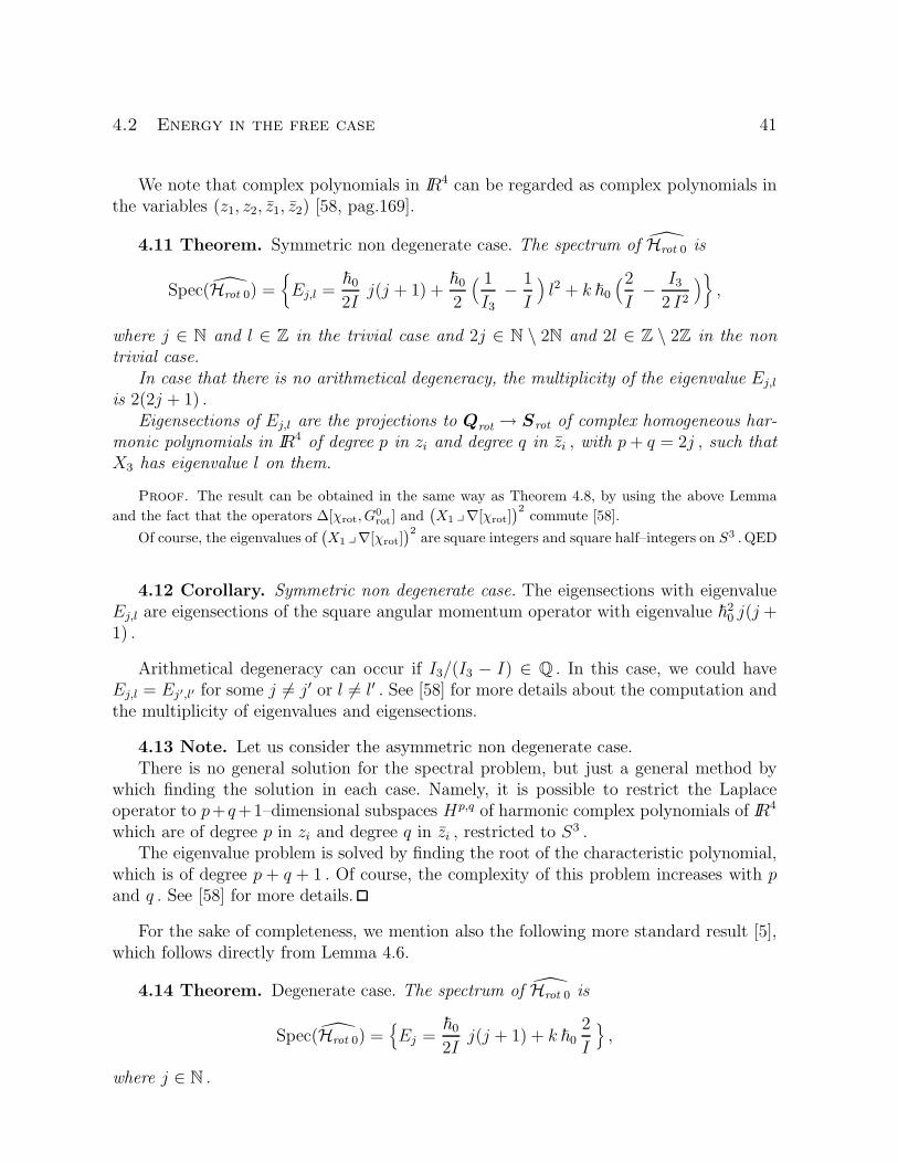
4.2 Energy in the free case 41
We note that complex polynomials in IR4 can be regarded as complex polynomials inthe variables (z1, z2, z1, z2) [58, pag.169].
4.11 Theorem. Symmetric non degenerate case. The spectrum of Hrot 0 is
Spec(Hrot 0) =Ej,l =
~0
2Ij(j + 1) +
~0
2
( 1
I3−
1
I
)l2 + k ~0
(2
I−
I32 I2
),
where j ∈ N and l ∈ Z in the trivial case and 2j ∈ N \ 2N and 2l ∈ Z \ 2Z in the non
trivial case.
In case that there is no arithmetical degeneracy, the multiplicity of the eigenvalue Ej,l
is 2(2j + 1) .Eigensections of Ej,l are the projections to Qrot → Srot of complex homogeneous har-
monic polynomials in IR4 of degree p in zi and degree q in zi , with p+ q = 2j , such that
X3 has eigenvalue l on them.
Proof. The result can be obtained in the same way as Theorem 4.8, by using the above Lemma
and the fact that the operators ∆[χrot, G0rot] and
(X1 y∇[χrot]
)2commute [58].
Of course, the eigenvalues of(X1 y∇[χrot]
)2are square integers and square half–integers on S3 . QED
4.12 Corollary. Symmetric non degenerate case. The eigensections with eigenvalueEj,l are eigensections of the square angular momentum operator with eigenvalue ~2
0 j(j +1) .
Arithmetical degeneracy can occur if I3/(I3 − I) ∈ Q . In this case, we could haveEj,l = Ej′,l′ for some j 6= j′ or l 6= l′ . See [58] for more details about the computation andthe multiplicity of eigenvalues and eigensections.
4.13 Note. Let us consider the asymmetric non degenerate case.There is no general solution for the spectral problem, but just a general method by
which finding the solution in each case. Namely, it is possible to restrict the Laplaceoperator to p+ q+1–dimensional subspaces Hp,q of harmonic complex polynomials of IR4
which are of degree p in zi and degree q in zi , restricted to S3 .The eigenvalue problem is solved by finding the root of the characteristic polynomial,
which is of degree p + q + 1 . Of course, the complexity of this problem increases with pand q . See [58] for more details.
For the sake of completeness, we mention also the following more standard result [5],which follows directly from Lemma 4.6.
4.14 Theorem. Degenerate case. The spectrum of Hrot 0 is
Spec(Hrot 0) =Ej =
~0
2Ij(j + 1) + k ~0
2
I
,
where j ∈ N .

42 4 Rotational quantum spectra
The multiplicity of the eigenvalue Ej is (2j + 1)2 .Eigensections of Ej are the harmonic complex polynomials in IR3 restricted to S2 of
degree 2j .
In this case, the system is again invariant under rotations and admits a momentummap which can be interpreted as the angular momentum. Proceeding in a similar way asabove we get
4.15 Corollary. Degenerate case. The eigensections with eigenvalue Ej are eigensec-tions of the square angular momentum operator with eigenvalue ~2
0 j(j + 1) .
4.3 Spectra with electromagnetic field
If the electromagnetic field does not vanish the computations of the spectramight become quite hard. However, specific problems can be faced.
Here, we sketch typical evaluations, with reference to the literature, showing howthey can be rephrased in our framework. Indeed, our non trivial bundle structureopens a possible geometric interpretation of the ‘two–valued’ wavefunctions, whichseems to be closely related to spin.
4.16 Example. (Stark and Zeeman effects.) The energy spectrum of a charged rigidbody rotating in a constant external electric, or magnetic field can be computed in ourframework along the lines of the previous section. The results fit the computations incoordinates that can be found in the literature [23, 10, 41, 47], but provide also a math-ematical framework for the half-integer part of the spectrum (which is usually discardedby invoking mathematical reasons).
For example, the energy eigenvalue equation in [23] can be reproduced by means of theanalysis of the electromagnetic field acting on a rigid system performed in section 2.3.6.In the case of trivial quantum bundle, the computation of the spectrum can be rephrasedword by word in our scheme. In the non trivial case, one should use half–integer valuesof angular momentum and repeat exactly the same computations.
In order to include in our scheme the anomalous Zeeman effect for a rigid body withspin rotating in a constant magnetic field, one should implement the spin in our covariantquantum mechanics according to [8].
4.17 Example. (Magnetic monopole). Let us consider a rigid body with a fixed pointat which a monopole is located. In this case we consider as electromagnetic pattern fieldthe field generated by the monopole. The main difference with the other examples ofelectromagnetic fields considered before is that the cosymplectic form Ω defines a non-trivial cohomology class. Therefore Ω does not admit global potentials. However, afterlifting all the structures to S3 (which is a fibration over Srot in both the non degenerateand degenerate cases), the quantum bundle becomes trivial and the computations areperformed very much in the same way as for the free rigid body. Another difference isthat the fixed point in the rigid body reduces the degrees of freedom to the rotational part.

4.3 Spectra with electromagnetic field 43
Therefore, in this case the analysis of the rotational part gives a complete description ofthe rigid body.
One of us [58] gave an exact solution to the spectral problem of a rigid rotator ina magnetic monopole field. We just recall that a magnetic monopole is a magnetic fieldwhich is proportional to the radial vector field in three–dimensional space.
Here follows the spectrum of the energy operator in the case of a symmetric rigidbody:
Spec(Hrot 0) =
Ej,l =
~0
2Ij(j + 1) +
~0
2
( 1
I1−
1
I
)l2 − ν0
‖~q‖
I3l +
ν20
~0
‖~q‖2
2I3+ k ρrot 0
,
where j ≥ 0 ,−j ≤ l ≤ j , j, l are integers, for the trivial quantum bundle, or half–integers,for the non trivial quantum bundle, ν is the magnetic charge of the monopole and ~q isthe center of charge of the monopole [58].

44 References
References
[1] R. Arens: A quantum dynamical, relativistically invariant rigid body system, Trans. A.M.S.147, (1970), 153–201.
[2] S. P. Baranovskii, V. V. Mikheev, I. V. Shirokov: Quantum Hamiltonian systems on
K-orbits: semiclassical spectrum of the asymmetric top, Teor. i Mat. Fiz. 129 n. 1 (2001),1311–1319.
[3] A. O. Barut, M. Bozic, Z. Mari’c: The Magnetic Top as a Model of Quantum Spin,Ann. of Phys. 214 (1992) 53–83.
[4] A. O. Barut, I. H. Duru: Path integral quantization of the magnetic top, Phys. Lett. A158 (1991), 441–444.
[5] M. Berger, P. Gauduchon, E. Mazet: Le Spectre d’une Variete Riemannienne, Lect.Not. Math. 194, Springer, 1971.
[6] R. Bot, L.W. Tu: Differential forms in algebraic topology, GTM 82, Springer–Verlag1982, Berlin.
[7] M. Bozic, D. Arsenovic: Quantum Magnetic Top, in “Quantization and Infinite–Dimensional Systems”, Eds.: J.–P. Antoine, Plenum Press, New York 1994, 223–229.
[8] D. Canarutto, A. Jadczyk, M. Modugno: Quantum mechanics of a spin particle in
a curved spacetime with absolute time, Rep. on Math. Phys., 36, 1 (1995), 95–140.
[9] H. Casimir: Rotation of a Rigid Body in Quantum Mechanics, Ph. D. Thesis, Wolters,Groningen 1931.
[10] J. H. Choi, D. W. Smith: Lower Bounds to Energy Eigenvalues for the Stark Effect in a
Rigid Rotator, J. Chem. Phys. 43, 10 (1965), S189–S194.
[11] C. Cohen–Tannoudji, B. Diu, F. Laloe: Quantum mechanics, vol. I and II, Interscience,1977.
[12] W. D. Curtis, F. R. Miller: Differentiable Manifolds and Theoretical Physics, Acad.Press, 1985.
[13] M. de Leon, G. M. Tuynman: A universal model for cosymplectic manifolds, J. Geom.Phys. 20 (1996), 77–86.
[14] H.–D. Doebner, H.–J. Mann: Vector bundles over configuration spaces: topological po-
tentials and internal degrees of freedom, J. Math. Phys. 38 (1997), 3943–3952.
[15] B. Dubrovine, S. Novikov, A. Fomenko: Geometrie contemporaine, Methodes et ap-plications, Vol. 1, 2, 3, Editions MIR, Moscou, 1979.
[16] C. Duval, J. Elhadad, M. J. Gotay, G. M. Tuynman: Nonunimodularity and the
quantization of the pseudo–rigid body, in “Hamiltonian Systems, Transformation Groupsand Spectral Transform Methods”, Eds.: J. Harnad and J. Marsden, Publications du CRM,Montreal 1990.
[17] A. Frolicher: Smooth structures, LNM 962, Springer–Verlag, 1982, 69–81.

References 45
[18] P. L. Garcıa: Cuantificacion geometrica, Memorias de la R. Acad. de Ciencias de Madrid,XI, Madrid, 1979.
[19] M. Gotay: Constraints, reduction and quantization, J. Math. Phys 27 (8) (1986), 2051–2066.
[20] M. Gotay: Obstruction to quantization, in “Proc. of the VII Conf. on Diff. Geom. and itsAppl.”, Brno 1998.
[21] T. Goto: Bohr–Sommerfeld’s Quantum Conditions and Rigid Body Rotation, Nuovo Cim.XXXI, 2 (1964) 397–401.
[22] V. Guillemin, S. Sternberg: Geometric Quantization and Multiplicities of Group Rep-
resentations, Inventiones Mathematicae 67 (1982), 515–538.
[23] J. Hajnal, G. Opat: Stark effect for a rigid symmetric top molecule: exact solution, J.Phys. B: At. Mol. Opt. Phys. 24 (1991), 2799–2805.
[24] A.J. Hanson, T. Regge: The relativistic spherical top, Ann. Physics, 87 (1974), 498-566.
[25] G. Herzberg: Molecular spectra and molecular structure I. Spectra of diatomic molecules,II. Infrared and Raman spectra of polyatomic molecules, Van Nostrand, New York, 1944.
[26] W. Hunziker: The Schrodinger eigenvalue problem for N -particle systems, Acta Phys.Austr., Suppl. XVII (1977), 43–71.
[27] T. Iwai: Classical and quantum mechanics of jointed rigid bodies with vanishing total an-
gular momentum, J. Math. Phys. 40, n. 5 (1999), 2381–2400.
[28] A. Jadczyk, M. Modugno: An outline of a new geometric approach to Galilei general
relativistic quantum mechanics,, in “Differential geometric methods in theoretical physics”,Eds.: C. N. Yang, M. L. Ge and X. W. Zhou, World Scientific, Singapore, 1992, 543–556.
[29] A. Jadczyk, M. Modugno: Galilei general relativistic quantum mechanics, Re-port of Department of Applied Mathematics, University of Florence, 1994, 1–215.http://www.dma.unifi.it/~modugno/
[30] J. Janyska, M. Modugno: Uniqueness Results by Covariance in Covariant Quantum
Mechanics, in “Quantum Theory and Symmetries”, Eds.: E. Kapuscik, A. Horzela, Proc. ofthe Second International Symposium, July 18–21, 2001, Krakow, Poland, World Scientific,London, 2002, 404–411.
[31] J. Janyska, M. Modugno: Covariant Schrodinger operator, Jour. Phys.: A, Math. Gen,35, (2002), 8407–8434.
[32] J. Janyska, M. Modugno: Covariant Quantum Mechanics, book in preparation, 2005.
[33] J. Janyska, M. Modugno: Hermitian vector fields and special phase functions, preprint,2005. http://arXiv.org/abs/math-ph/0507070
[34] J. Janyska, M. Modugno, D. Saller: Covariant quantum mechanics and quantum
symmetries, in “Recent Developments in General Relativity”, Eds.: R. Cianci, R. Collina,M. Francaviglia, P. Fre, Genova 2000, Springer–Verlag, Milano, 2002, 179–201.
[35] J. Janyska, M. Modugno, R. Vitolo: Semi–vector spaces, preprint 2005.

46 References
[36] G. John: On geometric quantization of the rigid body, in “Group theoretical methods inphysics”, Eds.: Wolf, Lect. Not. Phys. 135, 1980.
[37] S. Klimek-Chudy, W. Kondracki: On the θ-theories and the multivalued wave functions,Jour. Geom. Phys. 1 n.3 (1983), 1–12.
[38] S. Kobayashi, K. Nomizu: Foundations of differential geometry I - II, Interscience Pub-lishers, John Wiley & Sons, New York, 1969.
[39] I. V. Komarov: Remarks on Kovalevski’s top, J. Phys. A 34 (2001), 2111–2120.
[40] B. Kostant: Quantization and unitary representations, Lectures in Modern Analysis andApplications III, Springer–Verlag, 170 (1970), 87–207.
[41] L. Landau, E. Lifchitz: Mecanique quantique, Theorie non relativiste, Editions MIR,Moscou, 1967.
[42] R. G. Littlejohn, M. Reinsch: Gauge fields in the separation of rotations and internal
motions in the n–body problem, Rev. Mod. Phys. 69, 1 (1997), 213–275.
[43] R. G. Littlejohn, K. A. Mitchell: Gauge theory of small vibrations in polyatomic
molecules, in “Proc. conf. in honour of the 60th birthday of J. Marsden”, 408–428.
[44] P. Maraner: Monopole Gauge Fields and Quantum Potentials Induced by the Geometry
in Simple Dynamical Systems, Ann. of Phys. 246 (1996), 325–346.
[45] J. Marsden, T. Ratiu: Introduction to Mechanics and Symmetry, Texts in Appl. Math.17, Springer 1994.
[46] A. Martens: Quantization of an affinely-rigid body with constraints, Rep. Math. Phys. 51,n.2/3 (2003), 287–296.
[47] A. Messiah: Quantum Mechanics, vol. I and II, Dunod, 1959.
[48] M. Modugno, C. Tejero Prieto, R. Vitolo: Comparison between Geometric Quanti-
sation and Covariant Quantum Mechanics, in “Lie Theory and Its Applications in Physics -Lie III”, Eds.: H.-D. Doebner, V.K. Dobrev and J. Hilgert, Proc. of the Third InternationalWorkshop, 11 - 14 July 1999, Clausthal, Germany, World Scientific, London, 2000, 155–175.http://arXiv.org/abs/math-ph/0003029
[49] M. Modugno, R. Vitolo: The geometry of Newton’s law and rigid systems, preprint,2005.
[50] F. Pan, J. P. Draayer: Algebraic Solutions for the Asymmetric Rotor, Ann. of Phys.275 (1999), 224–237.
[51] M. Pavsic: Rigid particle and its spin revisited, http://arXiv.org/abs/hep-th/0412324
[52] M. Puta: On the dynamics of the rigid body with a single rotor and an internal torque,Rep. Math. Phys. 32, 3 (1993), 343–349.
[53] D. Saller, R. Vitolo: Symmetries in covariant classical mechanics, J. Math. Phys., 41,10, (2000), 6824–6842. http://arXiv.org/abs/math-ph/0003027

References 47
[54] A. K. S lawianowska, J. J. S lawianowski: Quantization of affinely rigid body in n
dimensions, Rep. Math. Phys 29 (1991), 297–320.
[55] J. Sniaticki: Geometric quantization and quantum mechanics, Springer–Verlag, New York,1980.
[56] J.–M. Souriau: Structures des systemes dynamiques, Dunod, Paris 1970.
[57] S. Tanimura, T. Iwai: Reduction of Quantum Systems on Rieman-
nian Manifolds with Symmetry and Application to Molecular Mechanics,http://arXiv.org/abs/math--ph/9907005.
[58] C. Tejero Prieto: Quantization of a rigid body in a magnetic monopole, Diff. Geom. andAppl., 14, (2001), 157–179.
[59] J. A. Toth: Eigenfunction localization in the quantized rigid body, J. Diff. Geom 43 (1997),844–858.
[60] M. Trunk: Algebraic Constraint Quantization and the Pseudo–Rigid Body,http://arXiv.org/abs/hep-th/9701112.
[61] R. Vitolo: Quantum structures in Galilei general relativity, Annales de l’Institut H.Poincare, 70, 1999.
[62] N. Woodhouse: Geometric quantization, 2nd Ed., Clarendon Press, Oxford, 1992.