a critical review of centrality measures in social networks
TRANSCRIPT

WI-
282
University of Augsburg, D-86135 Augsburg Visitors: Universitätsstr. 12, 86159 Augsburg Phone: +49 821 598-4801 (Fax: -4899) University of Bayreuth, D-95440 Bayreuth Visitors: F.-v.-Schiller-Str. 2a, 95444 Bayreuth Phone: +49 921 55-4710 (Fax: -844710) www.fim-rc.de
Discussion Paper
A Critical Review of Centrality Measures in Social Networks
by
Andrea Landherr, Bettina Friedl, Julia Heidemann1
1 At the time of writing this paper, Julia Heidemann was a research assistant at the Research Center Finance & Information Management and the Department of Information Systems Engineering & Financial Management at the University of Augsburg.
in: Business & Information Systems Engineering 2 (2010) 6, p. 371-385

A Critical Review of Centrality Measures in Social Networks Authors Andrea Landherr, Bettina Friedl, Julia Heidemann Social networks are currently gaining increasing impact especially in light of the ongoing growth of web-based services like facebook.com. A central challenge for the social network analysis is the identification of key persons within a social network. In this context, the article aims at presenting the current state of research on centrality measures for social networks. Given highly variable findings on the quality of various centrality measures, we also illustrate the tremendous importance of a reflected utilization of existing centrality measures. For this purpose, the paper analyzes five common centrality measures on the basis of three simple requirements for the behavior of centrality measures. Abstract Social networks are currently gaining increasing impact in light of the ongoing growth of web-based services like facebook.com. One major challenge for the economically successful implementation of selected management activities such as viral marketing is the identification of key persons with an outstanding structural position within the network. For this purpose, social network analysis provides a lot of measures for quantifying a member’s interconnectedness within social networks. In this context, this paper shows the state of the art with regard to centrality measures for social networks. Due to strongly differing results with respect to the quality of different centrality measures, this paper also aims at illustrating the tremendous importance of a reflected utilization of existing centrality measures. For this purpose, the paper analyzes five common centrality measures from literature on the basis of three simple requirements for the behavior of centrality measures. Key Words Social network, Interconnectedness, Centrality measures, Social network analysis 1 Introduction
Fundamental developments in information technology (IT) and especially the enormous growth of the
Internet are essential drivers for the increasing global interconnectedness of companies and
individuals. The targeted use of powerful IT thereby significantly facilitates the interaction of actors at
different locations and information exchange in real time. In this context, services subsumed under the
term Web 2.0, such as wikis, blogs, or online social networks, in which individuals are connected to
each other and share news, experiences, and knowledge, increasingly gain importance. The U.S.
market researcher Hitwise for instance reported in March 2010 that – as measured by the number of
visits – the online social network facebook.com replaced the search engine giant google.com as the
most visited U.S. website (Hitwise 2010). Moreover, according to a recent study by the Nielsen
Company about 66 % of global Internet users are actively using these new social communities each
month (The Nielsen Company 2009, p. 2). Given this development, it is not surprising that web-based
social networks have attracted the interest of many companies since a majority of their customers now
regularly uses these services and, in this way, exchanges on products and services (De Valck et al.
2009, p. 185).
The constitutive feature of social networks are the relationships between network members and hence
the network structure induced by the mutual connections (Zinoviev and Duong 2009). This
interconnectedness of an actor – i.e., his structural integration into the network – significantly
influences his communication and interaction, and therefore holds valuable information for companies
with regard to various corporate issues. Concerning viral marketing, for instance, the integration of
well-connected actors is of considerable importance in order to attract the attention of the largest

possible audience to a brand, a product, or a campaign (Kiss and Bichler 2008, p. 233; De Valck et al.
2009, p. 187). In product development and in particular in the identification of trends, the integration of
members who are taking a central position within their network is also of great advantage since these
actors have access to information on a variety of other actors (De Valck et al. 2009 S. 185).
The successful implementation of this exemplary list of business related issues and similar ones
requires the identification of those members (key persons) who are structurally very well integrated
into a social network. This identification is not only necessary for the success of business decisions,
but is particularly important in the context of time and budget constraints. In this context, taking
recourse to the social network analysis (SNA), which has already developed and discussed a variety
of centrality measures (CM) for the quantification of the interconnectedness of actors in social
networks, appears suitable. Therefore, the aim of this paper is (1) to show the current state of
research with regard to CM in social networks and (2) to illustrate the enormous importance of a
reflected utilization of existing CM in view of highly variable findings on the quality of various CM in
SNA.
The paper is organized as follows: In section 2, we first present the state of research on CM in social
networks. On this basis, we exemplarily formulate three simple general requirements for CM in section
3, which are used in section 4 to analyze five commonly applied CM from the literature on SNA. The
paper concludes with a summary of results and an outlook in section 5.
2 Social Networks
2.1 Structure and Characteristics of Social Networks
Based on Valente (1996) the term social network is understood in this paper as a "pattern of
friendship, advice, communication or support" (Valente 1996) between individual members or groups
of members within a social system (cf. also Burt and Minor 1983; Knoke and Kuklinski 1982; Scott
1991; Wellman 1988). Usually, a common goal, interest, or need of the various persons involved
constitutes the unifying element of such a network. Web-based social networks use the infrastructure
of the Internet to provide basic functionality for identity management (i.e., the presentation of oneself),
relationship management (i.e., managing one’s own contacts or cari the network), and visualization of
profiles and networks (Koch et al. 2007). In this way, the community feeling of the actors, which is a
central characteristic of such networks, can be achieved also without their direct physical presence
(Heidemann 2009). The features for relationship management and in particular the management of
contacts via contacts lists in web-based social networks especially enable maintaining casual
acquaintances which are often not kept alive in reality.
Taking a structural point of view, we can model the relationships within a social network as a graph G
with a set VG of nodes and a set EG of edges between these nodes. The set VG represents the
members of the social network, while the set EG refers to the relationships between them and thus
describes social ties and interaction potentials between the actors (Sabidussi 1966; Wassermann and
Faust 1994). The resulting network structure of a social network can also be represented by a matrix

A=(aij)∈{
entry axy
Fig. 1 Ex
Regardin
networks
overview
are one-
network)
Milgram
a surpris
phenome
both in th
and Milg
forms a
which ca
without
commen
relation w
social ne
homoge
al. 2006
highly in
individua
individua
that play
develope
CM in so
{0;1}nxn. The
y is 0. Fig. 1
xample of a s
ng the char
s (Newman a
w cf. Wasser
-sided relatio
) (Wasserma
realized alre
singly short c
enon", which
he offline an
gram 1969). G
single conn
an be analy
any relation
nts, however
with each ot
etworks are
neously acro
6; Mislove et
ntegrated me
al groups of
al members
y a central ro
ed within SN
ocial network
entry axy of
illustrates an
social netwo
racteristics o
and Park 200
mann and F
onships ((un
ann and Fa
eady in the 1
chain from a
h is also kno
d in the onlin
Given these
ected graph
yzed separa
nship to othe
r, focus on s
ther person
mostly sca
oss all memb
t al. 2007).
embers – so
f strongly int
of a social n
ole in a socia
NA. In the fol
ks.
this so-calle
n example of
ork
of social ne
03), we can
aust 1994). S
-)directed ne
aust 1994, p
960s that ev
n average o
own under th
ne world (e.g
findings we
. In addition
ately in term
er actors (K
social netwo
in a direct o
le-free netw
bers (e.g., B
Instead, in s
-called hubs
terconnected
network gene
al network it
llowing secti
ed adjacency
f the represe
tworks, whic
draw on a va
Social netwo
etwork) or d
p. 44). Furth
very person i
f six contact
he heading "
g., Dodds et
can assume
n, there migh
ms of interco
Kumar et al.
orks or those
r indirect wa
orks in whic
Barabási and
such networ
s (see Fig. 1d members.
erally differs
t appears ap
on we theref
y matrix is 1,
ntation of a s
ch highly di
ariety of exis
orks can e.g.
ifferent relat
hermore, the
is connected
ts (Milgram 1
"six degrees
al. 2003; Les
e that the maj
ht also be ot
onnectedness
. 2006; Misl
e subgraphs
ay. Furtherm
ch the numb
Bonabeau 2
rks many low
1) – exist. Th
Overall, the
significantly
ppropriate to
fore present
if (x,y)∈EG h
social networ
iffer from bi
sting knowled
be classified
ionship inten
e American
d to everyone
1967). This s
of separatio
skovec and H
jority of acto
ther smaller
s, as well a
love et al. 2
in which ea
ore, numero
ber of conta
2003; Ebel e
w-interconne
hese hubs a
e interconne
y. In order to
make use o
the state of
holds. Other
rk as a graph
iological or
dge from SN
d as to whet
nsities ((un-)
psychologist
e else in the
so-called "sm
on", can be o
Horvitz 2008
ors in a socia
groups of m
as isolated m
2007). The
ach person s
ous studies s
cts is not d
et al. 2002;
ected and on
act as a link
ctedness of
identify thos
of CM that ha
f research as
rwise, the
h.
technical
NA (for an
ther there
)weighted
t Stanley
world via
mall world
observed
8; Travers
al network
members,
members
following
stands in
show that
istributed
Kumar et
nly some
between
different
se actors
ave been
s regards

2.2 Interconnectedness and Centrality Measures in Social Networks
Since many years, the interconnectedness of actors in social networks has been a central issue of
SNA. Simplifying, the discussion is often limited to undirected, unweighted social networks. However,
even for these relatively simple graphs there is no uniform understanding of an actors’ centrality in a
social network (Borgatti and Everett 2006, p. 467). Instead, there are some very different concepts and
context-specific interpretations of the centrality of a node (Borgatti and Everett 2006, p. 467) that may
result from different objectives for the use of CM. In the following, we therefore firstly present four
basic concepts of centrality. In the simplest case, the number of a network member’s direct contacts is
a useful indicator of centrality. The advantage of this interpretation of an actor’s centrality, with degree
centrality (DC) as its standard representative (Nieminen 1974; Shaw 1954), is the relatively easy
interpretability and communicability of the results. A second approach is based on the idea that nodes
that have a short distance to other nodes and consequently may disseminate information on the
network very effectively are taking a central position in the network (Beauchamp 1965; Sabidussi
1966). A representative of this approach is closeness centrality (CC), where a person is seen as
centrally involved in the network if he requires only few intermediaries for contacting others and thus is
structurally relatively independent. Accordingly, the calculation of this CM includes the length of the
shortest paths to all other actors in the network. Further developments of CC even use the length of all
paths between the actors for the calculation (e.g., Newman 2005). A third approach, however, equates
centrality with the control of the information flow which a member of the network may exert based on
his position in the network. Thereby, it is assumed implicitly that the communication and interaction
between two not directly related actors depends on the intervening actors. The most prominent
representative of this concept is betweenness centrality (BC), where the determination of an actor’s
centrality is based on the quotient of the number of all shortest paths between actors in the network
that include the regarded actor and the number of all shortest paths in the network (Bavelas 1948;
Freeman 1977; Shaw 1954). The common characteristic of all networking concepts presented so far is
that only little or no attention is paid to indirect contacts, meaning they are not or only indirectly
included in the quantification of an actor’s centrality. This is where the so-called influence measures
come into play. These CM consider actors to be centrally involved in the network if their directly
connected network members stand in relation with many other well-connected actors. Some of the
best known of these recursively defined CM are the eigenvector centrality (EC) (Bonacich 1972), the
CM by Bonacich (Bonacich 1972), and the CM by Katz (Katz 1953). Besides these representatives of
the four basic concepts of centrality, a plethora of other CM has been defined over the years (see, e.g.
Bonacich and Lloyd 2001; Freeman et al. 1991; Lee et al. 2009; Rousseau and Zhang 2008) which,
e.g., enable the integration of edge weights or of directional connections or are suitable for specific
applications and network types. Usually, these CM represent modifications or enhancements of the
already discussed CM and thus are not elaborated in more detail in this article. For the mathematical
calculation of each CM different algorithms have been developed which may vary significantly in terms
of complexity. While the DC only requires to count the direct contacts of the n nodes in the network
(complexity of O(n)), the complexity of BC in unweighted graphs amounts to O(n·m) (Brandes 2001),

where m is the number of edges in the network.1 At the same time, this algorithm allows the
calculation of other distance-based CM, such as CC, for which Okamoto et al. (2008) discuss other
algorithms and heuristics. According to Kiss and Bichler (2008), the complexity of calculating the EC is
O(n2), whereas in case of Katz’s CM the inverting of the adjacency matrix initially induces a complexity
of O(n3). However, this complexity can be reduced by applying the algorithm of Coppersmith and
Winograd (1990) to O(n2.376).
Starting from the definition of different CM a lively discussion on the characteristics and the robustness
(e.g., in case of incorrect or incomplete data on the network structure) of different CM arose.
Accordingly, on the one hand, there exist numerous empirical studies that discuss the application of
CM using different real or simulated networks. On the other hand, much research exists which –
starting from the concept of different CM – derive conclusions about their properties or suitability for
different applications. Tab. 1 provides an overview of relevant contributions, which are classified
according to the dimensions of focus (empirical vs. conceptual), approach, and analyzed CM.
In the field of applying CM to real or simulated networks, e.g., Bolland (1988) discusses the
robustness of DC, CC, BC, and the CM by Bonacich in random and systematic variation of the
underlying network structure. This analysis shows that BC is generally very unstable with regard to the
variation of the network structure. In contrast, for DC and CC the centrality score usually varies only a
little in case of a random or systematic change of the underlying network structure. However,
according to the studies of Bolland (1988) the CM of Bonacich is the least sensitive one in terms of a
random or systematic variation of the network structure. A further contribution to the discussion on the
robustness of different CM is provided by Borgatti et al. (2006) who first define four different types of
error (adding or deleting an edge or a node) and then compare the CM DC, CC, BC, and EC with
regard to these different types of errors. The main finding of the study is that the four CM react very
similarly to manipulations of the network structure, with BC being a little bit worse than the other three.
Frantz et al. (2009) extend these investigations by differentiating five network topologies. They
conclude that the robustness of the four CM also depends on the particular topology of the network.
Furthermore, Costenbader and Valente (2003) also analyze the stability of different CM in presence of
incorrect or incomplete information on the structure of a network (e.g., for the analysis of a sample of
the network). In addition to the classic CM DC, CC, BC, EC, and the CM by Bonacich, their
investigation includes two more CM and they also extend their analysis to directed graphs. For
undirected, unweighted social networks they come to the conclusion that the centrality scores of
individual actors, which have been determined based on a sample of the overall network, have the
highest average correlations with the centrality scores of the individual actors in the overall network in
the case of EC (before DC, CC, and BC). Here, BC, however, comes off less successfully than the
other three CM, indicating a fundamentally distinct conception of centrality for this CM (Bolland 1988).
The investigations on the robustness of CM concerning the variation of the network structure
discussed here are very important since the connections between actors that are considered for an
analysis of social networks usually only present a distorted picture of the real social network for both
the offline and the online context. Therefore, using CM one is often confronted with the problem of 1 If an approximation rather than a precise calculation of the values of BC is sufficient, the faster algorithm of Bader et al. (2007) can be used.

incomplete information on the structure of the network or does not have the resources necessary to
measure the structure of large, complex networks in total. Therefore, the information on the
robustness of the used CM is highly relevant.
Tab. 1 Approaches to the Analysis of Centrality Measures
Authors Focus Approach Analyzed Centrality Measures
Bolland (1988)
conceptional & empirical
Analysis of the robustness and sensitivity of different centrality models under conditions of random and systematic variation introduced into a network
DC, CC, BC, CM by Bonacich
Borgatti (2005) conceptional
Discussion of various CM regarding their matching for different types of network flow
DC, CC, BC, EC
Borgatti et al. (2006) empirical Analysis of the robustness of CM under
conditions of imperfect data DC, CC, BC, EC
Costenbader and Valente
(2003) empirical Analysis of the stability of centrality
measures when networks are sampled
DC, CC, BC, EC, CM by Bonacich, Integration, Radiality
Freeman (1979) conceptional & empirical
Discussion of different concepts of centrality and application of related CM to different exemplary networks
DC, CC, BC
Freeman et al. (1980)
conceptional & empirical
Identification of an appropriate CM for the case of problem solution in groups DC, CC, BC
Gneiser et al. (2010) conceptional Development of requirements for a CM
for online social networks DC, CC, BC, PageRank-based CM
Kiss and Bichler (2008) empirical
Comparison of the performance of different CM regarding the identification of influencers in a network of calls from a telecom company
DC, CC, BC, EC, PageRank-based CM, Edge-weighted DC, HITS-based CM, SenderRank CM
Mutschke (2008) conceptional Discussion of various anomalies of CM DC, CC, BC
Nieminen (1974) conceptional Development of axioms for CM DC
Sabidussi (1966) conceptional Development of axioms for CM Various indices
Besides considerations on the robustness of different CM there is further research which identifies and
analyzes the differences in results when applying different CM. Mutschke (2008), for instance,
describes six anomalies (i.e., high centrality score of an actor using one CM but low centrality score
when using other CM at the same time) when applying the CM DC, BC, and CC and gives a possible
justification for each of these differences in the centrality of an actor. Further contributions focus on the
partly significant differences in the rankings of the different actors in a social network when using
different CM (e.g., Freeman 1979; Freeman et al. 1980; Kiss and Bichler 2008). Here, the ranking of
the actors is defined by the descending order of the centrality score of the respective CM. In this
context, when comparing the CM DC, CC, and BC for all possible graphs with five actors, Freeman
(1979) e.g. concludes that the order of the different actors varies enormously using different CM. This

observation is also confirmed by the work of Freeman et al. (1980), in which the CM DC, CC, and BC
are applied to other sample networks. In addition, this article evaluates the suitability of the three CM
to identify key persons in the context of "problem solving in groups". More recent contributions deal
with the capability of different CM for other applications (e.g., Borgatti 2006; Hossain et al. 2007; Kiss
and Bichler 2008; Lee et al. 2010; Gloor et al. 2009). For example, Kiss and Bichler (2008) investigate
the quality of different CM in terms of news dissemination in a telecommunications network. Their
analysis is based on a defined diffusion model. In addition to the classic CM DC, CC, BC, and EC the
authors also apply newer concepts (such as PageRank-based CM, the edge-weighted DC, a HITS-
based CM and a SenderRank CM) (Kiss and Bichler, 2008, pp. 236 f.). The main result of this
investigation is that the centrality of individual actors significantly differs when using various CM, with
the SenderRank CM and the relatively simple CM out-degree (a directed version of the DC) being
suited best for the identification of key persons in this application case. Hossain et al. (2007) consider
a similar issue by evaluating real-world data from the mobile sector as regards the four CM DC, CC,
BC, and EC in order to assess the relationship between the centrality of an actor and his possibilities
for disseminating information. It turns out that only by combining different CM the most important
actors for the dissemination of information can be identified. Lee et al. (2010) deal with a related
problem and analyze the suitability of the CM DC and BC as an indicator for the influence of individual
customers on the behavior of the entire customer base. For this purpose, the authors conduct various
field studies and evaluate the involved actors’ self-assessment and the assessment by others in terms
of their influence on other clients. The analysis shows that the BC is in both cases positively related to
opinion leadership, whereas out-degree centrality is only a good indicator in terms of self-assessment
of the surveyed actors. Moreover, Borgatti (2006) examines the quality of CM for the identification of
key individuals for the purpose of optimally diffusing something through the network on the one hand
and for the purpose of disrupting or fragmenting the network by removing nodes on the other hand.
The author concludes that the traditional CM CC is suited best for the first case, while in the second
case BC is preferable. Since these CM do not exhaustively solve the particular problems, Borgatti
(2006) additionally developed new CM that are better suited for the studied issues. Comparing the
results of current research on analyzing the centrality of individual actors in the application of various
CM as discussed above, it remains to be noted that different CM in some cases lead to considerably
different results in terms of the centrality of individual actors.
In addition to the previously discussed empirical work there are also some conceptual studies in the
SNA on the characteristics and underlying assumptions of CM. Bolland (1988) explains for each of the
CM DC, CC, and BC and the CM by Bonacich two assumptions on the nature of network flow, one
concerning the decay of resources (such as information) over distance and time and the other
concerning the paths through which resources are able to flow. He comes to the conclusion that
different CM are implicitly based on different assumptions on the losses that incur in transferring a
resource from one actor to another. While the DC assumes immediate deterioration of the transferred
resource after a transfer starts, BC and Bonacich’s CM assume no deterioration of the resource. In
case of CC, however, a gradual loss of the resource with increasing number of transfers is assumed.
Also Borgatti (2005) discusses different possibilities of network flow using some example cases for CM
and assigns appropriate CM to them. However, this assignment in Borgatti (2005) is merely

argumentative, i.e. he does not provide quantitative criteria for intersubjective verification of the
suitability of individual CM for certain applications. Other authors (e.g., Nieminen 1974; Sabidussi
1966) approach the question of the quality of a CM through the formulation of axiomatic requirements
on the characteristics and the behavior of CM. Also for the special case of online social networks first
contributions exist, aiming at a stronger focus on the characteristics (e.g., high relevance of indirect
contacts of an actor) of these web-based social networks when deriving requirements for a CM in
order to quantify the centrality of individual actors (see, e.g., Gneiser et al. 2010). However, this
research largely lacks the motivation or justification for why and in which cases the CM should meet
the requirements. Moreover, these requirements are partly of qualitative nature so that an
intersubjective assessment of their validity for different CM is difficult.
In summary, we can note that recent research on interconnectedness and CM in social networks has
defined different concepts of centrality and, based on these concepts, has developed different CM.
Furthermore, there are a number of both empirical and conceptual papers which compare different CM
and discuss their suitability for various applications, network types, and network flows. In this context,
the respective authors aim at the presentation and discussion of anomalies of different CM on the one
hand or at the identification of the CM that is most appropriate for the particular application case or
network flow on the other hand. In addition, the analysis of current research shows that different CM in
some cases provide considerably different results in terms of the centrality of individual actors.
Therefore, the selection of a CM requires the consideration of both the specifics of different CM and
the widely varying requirements of different application cases. Given the highly variable findings in
view of quality of different CM, this article focuses on the illustration of the enormous importance of a
reflective use of CM. Based on the findings of the SNA literature, in the following section we motivate
and formulate three simple general, quantitative, and thus intersubjectively testable properties of CM
in social networks, partly drawing on the work of Nieminen (1974) and Sabidussi (1966). The three
properties are then used for the analysis of some of the most widely discussed and used CM of SNA.
3 Properties of Centrality Measures in Social Networks
Formally, a measure to quantify interconnectedness of a node x in a graph G is a mapping
σG:VG→IR0+ which assigns a non-negative real number to each x∈VG, where a higher value of σG
indicates a better interconnectedness. In case of an identical network structure of two nodes x and y in
the network the application of the CM should have the same value σG(x)=σG(y) for both nodes
(Nieminen 1974, p. 333; Sabidussi 1966, p. 592). Two nodes x and y are thereby considered as being
identically structurally integrated into the network if a renaming of all nodes of the network is possible
in such a way that all existing edges remain and x is mapped to y, i.e. if an automorphism2 η:VG→VG
with y=η(x) exists. In Fig. 2, e.g., the nodes 1 and 5 as well as the nodes 2 and 4 are identically
integrated into the network in terms of structure since these nodes can be each mapped to each other
through 2→4, 4→2, 3→3, 1→5, 5→1 and the edges (1,2) (4,5) (2,3) (3,4) and (2,4) remain.
2 An automorphism is an isomorphism of a graph to itself, with two graphs G=(VG,EG) and G’=(VG’,EG’)
being referred to as isomorphic if a bijection η:VG→VG’ exists with (a,b)∈EG if and only if (η(a),η(b))∈EG’ for all a, b∈VG.

Fig. 2 Example of a network illustrating structural equivalence
In the subsequent motivation of three simple general properties of CM in undirected, unweighted
social networks we always assume a connected graph G. Furthermore, statements about the desired
behavior of a CM when adding a new edge are made. Thus, the network is transformed from a state 1
(with associated graph G) in a state 2 (with associated graph G‘). The removal of an edge exactly
corresponds to the opposite operation and is associated with the reversal of the statement. For this
reason, we only consider the case of adding an edge in the following.
With an additional relationship between a member x and another member y in the network the
opportunities for communication and interaction particularly increase if x gains a more direct
connection (i.e. of lesser distance dG(x,y)) to y. The distance dG(x,y) between the actors x and y is
thereby defined as the minimum length of all paths in G that lead from x to y. In this context, Davis
(1969, p. 549) assumes that the flow of information between two actors decreases in proportion to
their connection length. Thus, both the volume and the quality of the transmitted information between
two actors are usually higher the smaller their distance is. In addition, with a relatively low number of
contacts between two actors the contacting is normally faster and the individual actors tend to have a
higher willingness to disclose relevant information (Algesheimer and von Wangenheim 2006).
Moreover, trust in the message passed through the network is usually higher in the case of a greater
closeness of the actors to each other. Overall, an actor x thus holds a higher potential in terms of
information exchange in the presence of a more direct connection to an actor y than without the
additional connection. This should be positively reflected in the value of the CM of x, as expressed in
the following property one:
Property 1 [Monotonicity with respect to the distance of the actors]
If the distance of the actor x to at least one other actor y is reduced through an additional relationship in the network, the centrality score of x increases.
Formally, this means:
If VG=VG‘, v, w, x, y∈VG, v≠w, x≠y, (v,w)∉EG, EG‘=EGυ(v,w) and if for the distance between x and y due to the additional relationship between v and w dG‘(x,y)<dG(x,y) holds, it follows that σG‘(x)>σG(x).
Due to the symmetry of relations in this case it also follows that σG‘(y)>σG(y).
Furthermore, it is advantageous for the interaction in a social network if an actor can contact another
member on various paths (Davis 1969, p. 549). In this way, disruptions of the information flow along a
single path can be compensated on the one hand. On the other hand, the actor usually receives more
information on different paths from and about a larger number of indirect contacts. In addition, several
paths to another member generally contribute to trust. This is due to the fact that in this case several,
more direct contacts of an actor have a relationship to this member and thus independently indicate
his trustworthiness. Due to the benefits of a smaller distance between two actors, as already described

above, a path is more valuable the shorter it is. If there are multiple paths of shortest length from one
network member to another, this actor also becomes more independent from the influence of
individual actors in between (Freeman 1979, p. 221). Hence, an increase in the number of paths with
shortest length should positively affect the centrality score of x. This is stated in the following property
two:
Property 2 [Monotonicity with respect to the number of shortest paths]
If the number of paths with shortest length from an actor x to at least one other actor y increases through an additional relationship in the network, the centrality score of x increases.
Formally, this means:
If VG=VG’, v, w, x, y∈VG, v≠w, x≠y, (v,w)∉EG, EG’=EGυ(v,w) and if for the distance between x and y due to the additional relationship between v and w dG‘
(v,w)(x,y)=dG(x,y)3 holds, it follows that σG‘(x)>σG(x).
Due to the symmetry of relations in this case it follows that σG‘(y)>σG(y).
Based on the assumption of symmetrical relations, an additional relationship between the actors x and
y is always advantageous for both parties involved as they possibly gain a better access to the
network of each other due to the new relationship. If actor x was previously connected better than
actor y, so it is expected that this ranking of the actors in terms of their centrality score remains the
same after adding the new contact. This results from the fact that actor y can benefit from the network
of actor x at most to the same extent as x does, since x still has a more direct access to his (better
evaluated) network than y and vice versa. This is expressed through the following property three:
Property 3 [Receipt of the actors’ ranking]
With an additional relationship between two actors x and y the ranking of the two members does not change with respect to the CM.
Formally, this means:
If VG=VG’, x, y∈VG, x≠y, σG(x)>σG(y), (x,y)∉EG, EG’=EGυ(x,y) holds, it follows that σG‘(x)≥σG‘(y).
If even σG(x)=σG(y) holds, it follows that σG‘(x)=σG‘(y).
The properties 1 to 3 represent three simple general requirements for the behavior of CM in social
networks which may be desirable in various applications. In section 4 we now analyze some
representatives of the CM already presented in section two in more detail.
4 Analysis of Centrality Measures
In the following we at a time first formally define five CM and illustrate them by means of an example
network. Afterwards we analyze them with respect to the previously formulated properties. The
selection is limited to DC, CC, and BC as well as the two influence measures EC and the CM by Katz
being some of the most commonly used CM in SNA literature and thus provides a cross section of the
different basic concepts of centrality as presented in section two.
4.1 Degree Centrality
3 Here, dG‘
(v,w)(x,y) refers to the length of the shortest path between x and y which contains the edge (v,w). Since the path with the length dG‘
(v,w)(x,y) only exists after adding the edge (v,w), the number of shortest paths really increases in the case dG‘
(v,w)(x,y)=dG(x,y).

The DC σD represents the simplest CM and determines the number of direct contacts as an indicator
of the quality of a network member’s interconnectedness (Nieminen 1974, p. 333). Using the
adjacency matrix A=(aij) it can be formalized as follows:
∑=
=n
iixD ax
1)(σ (1)
As a consequence, the centrality score σD(x) for a node x is higher, the more contacts a node x has. In
the network of Fig. 3, e.g., it follows that σD(1)=1 since actor 1 has only one direct relationship with
actor 2. In contrast, actor 4 has a centrality score σD(4)=3.
Fig. 3 Example of a Network for the Illustration of Centrality Measures
Tab. 2 shows the values of the DC for all members of the example network. In addition, the actors’
ranking (in short "rank") is stated, i.e. their order in descending value of the DC. The actors 2, 4, 6, and
7 take rank 1 and thus are the best networked members when applying this CM.
Tab. 2 Results for Degree Centrality
Degree Centrality
Actor x 1 2 3 4 5 6 7 8 9 10
σD(x) 1 3 2 3 2 3 3 1 2 2
Rank 9 1 5 1 5 1 1 9 5 5
With respect of the properties 1 to 3 the major disadvantage of the DC is that indirect contacts are not
considered at all. Therefore, a reduction of the distance from one actor x to another actor y resulting
from an additional relationship in most cases does not increase the value of the CM.4 The
intensification of a connection of shortest length between x and y does also not increase the value of
this CM, since the DC only considers direct contacts. However, in an undirected, unweighted graph a
direct connection between the actors x and y can exist only once. Overall, the properties 1 and 2 are
therefore not met in general. In contrast, the DC satisfies property 3. Through a new relationship both
actors involved win one additional direct contact. So the DC of both members equally increases by 1
and the ranking of the actors, thus, always remains the same.
4.2 Closeness Centrality
4 An exception is the case that the new edge (x,y) is added and dG’(x,y)=1 results.

The CC σC is based on the idea that nodes with a short distance to other nodes can spread
information very productively through the network (Beauchamp 1965). In order to calculate the CC
σC(x) of a node x the distances between the node x and all other nodes of the network are summed up
(Sabidussi 1966, p. 583). By using the reciprocal value we achieve that the value of the CC increases
when reducing the distance to another node, i.e. when improving the integration into network.
Formally, this means (e.g., Freeman 1979, p. 225)
∑=
= n
i G
Cixd
x1
),(1)(σ (2)
For actor 4 in the network of Fig. 3 σC(4)=1/21 results. This is due to the fact that for the actors
x=2, 3, 5 dG(4,x)=1, for the actors x=1, 6 dG(4,x)=2, for the actors x=7, 10 dG(4,x)=3 and for the actors
x=8, 9 dG(4,x)=4 holds. Tab. 3 includes the centrality scores of all members in the network from Fig. 3
and their ranking when applying the CC.
Tab. 3 Results for Closeness Centrality
Closeness Centrality
Actor x 1 2 3 4 5 6 7 8 9 10
σC(x) 1/34 1/26 1/27 1/21 1/19 1/19 1/23 1/31 1/29 1/25
Rank 10 6 7 3 1 1 4 9 8 5
For the CC the shortening of the distance to at least one other actor when adding an additional
relationship leads to a smaller value of the denominator in formula (3). Consequently, in this case the
value of the CM of the considered actor increases and property 1 is satisfied. However, in formula (3)
only the distances between the different actors are taken into account. Therefore, a larger number of
paths with shortest length between two actors does not positively affect the value of this CM as
illustrated by the network 4a, where both before and after adding the additional connection (3,4)
σCG(1)=σC
G’(1)=1/4 holds, although in G' there are two paths of length 2 from actor 1 to actor 3. In the
network 4b the ranking of the actors 1 and 2 also changes. While initially σCG(1)=1/13=σC
G(2) holds,
σCG’(1)=1/10<σC
G’(2)=1/9 results after adding the connection (1,2). Consequently, property 3 is also
not fulfilled.
Network 4a Network 4b
Fig. 4 Closeness Centrality – Counterexamples to Property 2 and 3

4.3 Betweenness Centrality
In case of the BC σB a network member is considered to be well connected if he is located on as many
of the shortest paths between pairs of other nodes. The underlying assumption of this CM is that the
interaction between two non-directly connected nodes x and y depends on the nodes between x and
y. According to Freeman (1979, p. 223) the BC σB(x) for a node x is therefore calculated as
∑ ∑≠= ≠<=
=n
xii
n
xjijj ij
ijB g
xgx
,1 ,,1
)()(σ (3)
with gij representing the number of shortest paths from node i to node j, and gij(x) denoting the number
of these paths which passes through the node x.
For actor 9 in the network of Fig. 3, e.g., σB(9)=1/2+1/2=1 results since he is located on one of the two
shortest paths from the actors 7 and 8 to actor 10. The values of the BC for the other actors and their
ranking are listed in Tab. 4.
Tab. 4 Results for Betweenness Centrality
Betweenness Centrality
Actor x 1 2 3 4 5 6 7 8 9 10
σB(x) 0 8 0 18 20 21 11 0 1 6
Rank 8 5 8 3 2 1 4 8 7 6
The BC does not meet any of the required properties as is demonstrated by the networks of Fig. 5. In
the network 5a actor 1 has a centrality score of σBG(1)=3 before adding the connection (4,5) and a
centrality score of σBG’(1)=1 afterwards, although the distance to actor 4 is reduced through the new
relationship. Consequently, property 1 is violated. Network 5b shows that property 2 is also not
satisfied for BC. For actor 1 holds first σBG(1)=2 and after adding the connection (3,4) σB
G’(1)=0,5
although there are two paths of length 2 from actor 1 to actor 3 due to the additional relationship.
Moreover, the ranking of the actors 1 and 2 changes in network 5c. While both have the same
centrality score (σBG(1)=0=σB
G(2)) before adding the connection (1,2), afterwards
σBG’(1)=1,5>σB
G’(2)=0,5 holds. Consequently, property 3 is also not fulfilled for BC.
Network 5a Network 5b Network 5c
Fig. 5 Betweenness Centrality – Counterexamples to Property 1 to 3

4.4 Eigenvector Centrality
The EC σE is based on the idea that a relationship to a more interconnected node contributes to the
own centrality to a greater extent than a relationship to a less well interconnected node. For a node x,
the EC is therefore defined as (Bonacich and Lloyd 2001)
∑=
⋅⋅==n
jjjxxE va
Avx
1max )(1)(
λσ (4)
with v=(v1,…,vn)T referring to an eigenvector for the maximum eigenvalue5 λmax(A) of the adjacency
matrix A.
In Tab. 5 the values of the EC for the actors 1 to 10 in the network of Fig. 3 and the resulting ranking
of the actors are listed.
Tab. 5 Results for Eigenvector Centrality (with λmax(A)=2,41)
Eigenvector Centrality
Actor x 1 2 3 4 5 6 7 8 9 10
σE(x) 0,171 0,413 0,363 0,463 0,342 0,363 0,292 0,121 0,221 0,242
Rank 9 2 3 1 5 3 6 10 8 7
Just like the BC, the EC does not meet any of the required properties. This can be illustrated by
means of the networks from Fig. 6.6 In network 6a, actor 1 first has a centrality score of σEG(1)=0,602
and after adding the connection (4,6) of σEG’(1)=0,417 although the distance of actor 1 to actor 6 has
been reduced. This contradicts property 1. In network 6b the value of the CM decreases for actor 4
when adding the new connection (1,2) (σEG(4)=0,604>σE
G’(4)=0,530) although the relationship
between actor 4 and actor 2 has been intensified. Therefore property 2 is also not fulfilled. Regarding
property 3, network 6c can serve as a counterexample. Whereas before adding the connection (4,6)
actor 4 has a lower centrality score than actor 6 (σEG(4)=0,271<σE
G(6)=0,311), the ranking of both
actors changes due to the new relationship (σEG’(4)=0,435>σE
G’(6)=0,421). Even these simple example
networks demonstrate the additional problem that the results of the EC are harder to interpret and less
comprehensible than those of the previously described CM.
5 Being a non-negative, irreducible matrix, A always has a positive eigenvalue, which is equal to the spectral radius, and an associated eigenvector with only positive entries (Graham 1987, p. 131). 6 For detailed calculations and further details, see Appendix A.

Network 6a Network 6b Network 6c Fig. 6 Eigenvector Centrality – Counterexamples to Property 1 to 3
4.5 Katz’s Centrality Measure
According to Katz not only the number of direct connections but also the further interconnectedness of
actors plays an important role for the overall interconnectedness in a social network (Katz 1953).
Therefore, Katz includes all paths of arbitrary length from the considered node x to the other nodes of
the network in the calculation of his CM σK. The CM by Katz for the node x is thus defined as
xi
iiTK eAkx ⎟
⎠
⎞⎜⎝
⎛= ∑
∞
=11)(σ (5)
with 1=(1,1,...,1,1)T representing the nx1 vector consisting of ones only and ex=(0,..,0,1,0,...,0)T the
unit vector as well as k an arbitrary (usually positive) weighting factor.7 Since the corresponding
adjacency matrix A=(aij) only contains the values 0 and 1, the entry ãxy of the matrix Ã=Ai represents
the number of paths of length i from x to y (Katz 1953, p. 40). For the convergence of the series, k
must be smaller than the reciprocal value of the maximum eigenvalue λmax(A) of the adjacency matrix
A (Katz 1953, p. 42). This simplifies σK to
( ) xnnT
K eIkAIx −−= −1)(1)(σ (5’)
with In referring to the identity matrix of the dimension n=|VG|. The weighting factor k can then be
sometimes interpreted as the probability that a single relationship is useful for node x. This results
(assuming independence of probabilities) in a probability of k2 for a relation of second degree, and so
forth (Katz 1953, p. 41). In Tab. 6, the values of the CM by Katz and the resulting rankings for the
actors 1 to 10 of the example network from Fig. 3 are listed.
Tab. 6 Results for the Centrality Measure by Katz (with k=1/3, λmax(A)=2,41)
Centrality Measure by Katz
Actor x 1 2 3 4 5 6 7 8 9 10
σK(x) 1,91 4,72 3,99 5,25 4,06 4,91 4,30 1,77 3,23 3,38
Rank 9 3 6 1 5 2 4 10 8 7
In each case the CM by Katz meets the properties 1 and 2 since adding any new relationship in a
connected graph always leads to an increase in the interconnectedness of all actors in the network.
This is due to the fact that in a connected graph, a new relationship for any actor opens up additional
paths to all other actors in the network. The validity of the third property for the CM of Katz can be
7 In contrast to the work of Katz we abstain from normalizing the column sum of the adjacency matrix by multiplication with 1/(n-1). As a consequence, the result differs by a multiplicative constant from the outcome in the original work by Katz. In addition, under the assumptions described here, the CM by Katz differs only by a constant of the alpha centrality. Further details are outlined in Appendix B.

proven formally only under certain conditions. However, extensive simulation studies show that the
ranking of two actors in the CM σK does not change by adding an additional relationship.8
4.6 Summary and Comparison of Analysis Results
Tab. 7 summarizes the resulting rankings of the actors when applying the five considered CM to the
example network in Fig. 3. It becomes obvious that the actors 1 and 8 have the worst centrality scores
for all CM investigated. Apart from this, however, there are significant differences regarding the actors’
rankings when using different CM. Actor 3, for instance, is seen as poorly interconnected when
applying BC or CC, while he ranks in the midfield using the DC or the CM by Katz and reaches a top
position when applying the EC. In addition, it is striking that DC and BC generally do not sufficiently
differentiate the interconnectedness of individual members. Thus, e.g., the DC provides the same
value for the actors 2, 4, 6, and 7 although with all other CM the actors 4 and 6 are seen as (partly
significantly) better interconnected than actor 7. This is due to the fact that the DC only considers the
number of direct contacts and not their further interconnectedness (i.e., their indirect contacts). In
addition, the BC does not distinguish between actors who have only one contact and actors whose
contacts are completely interconnected. In both cases, such actors have an centrality score of 0 and
thus the last rank (see, e.g., actors 1, 3, and 8). This analysis shows that an actor’s centrality score
can vary considerably depending on the CM.
Tab. 7 Ranking Applying Different Centrality Measures
Rank Degree Centrality
Betweenness Centrality
Closeness Centrality
Eigenvector Centrality
Centrality Measure by
Katz 1 2, 4, 6, 7 6 5, 6 4 4
2 5 2 6
3 4 4 3, 6 2
4 7 7 7
5 3, 5, 9, 10 2 10 5 5
6 10 2 7 3
7 9 3 10 10
8 1, 3, 8 9 9 9
9 1, 8 8 1 1
10 1 8 8
Tab. 8 summarizes the results regarding the validity of the three properties for all CM presented in this
paper. It shows that the majority of the frequently used CM in SNA literature does not or not fully meet
the properties discussed in this article. Both the BC and EC, for instance, satisfy none of the desired
properties, while the DC and CC only fulfill one of the three properties. According to the findings of the
authors so far, among the five CM considered in this paper, only the CM by Katz meets all three
properties. However, the validity of the third property could only be validated by a simulation study
8 For detailed descriptions see Appendix C.

(see App
relatively
supplem
may ofte
responsi
its limita
regardin
Tab. 8 A
Ce
D
Betw
Clo
Eige
Centra
5 Summ
The com
major ca
proportio
induces
selected
of actors
many C
currently
state of
reflected
different
The pap
individua
the und
contribut
contribut
results f
network.
this cont
various a
surprisin
pendix C). T
y generic,
mentary relati
en lead to n
ible decision
ations. A CM
g the require
Analysis of C
entrality Me
Degree Centr
weenness Ce
oseness Cen
envector Ce
ality Measur
mary and Ou
mprehensive
auses of fund
on of the
k.com has a
an increase
activities in
s who are str
M have bee
y high import
research re
d use of the
CM.
er shows tha
al actors in s
erlying conc
tions analyzi
tions from SN
for the centr
. Furthermor
text, this pap
applications.
ngly only one
This result is
intuitively p
onship betw
not consider
n makers sho
M thus should
ements resul
entrality Mea
asure
rality
entrality
ntrality
entrality
re by Katz
utlook
IT penetrat
damental ch
world popu
about 400 m
e in the numb
areas such a
ructurally we
en developed
tance of web
garding CM
existing CM
at in the SNA
social netwo
cept of cen
ng and comp
NA literature
rality of indiv
re, depending
per exemplar
On the bas
e of the stud
all the more
plausible req
een two acto
red and pos
ould always
d not be sele
ting from the
asures – Sum
Prope
ion in all are
hanges in co
lation is ac
million mem
ber of comp
as marketing
ll integrated
d and discu
b-based socia
in social ne
in social ne
A literature a
orks. Thereby
trality. In ad
paring the pr
one can con
vidual actors
g on the app
rily presents t
sis of these p
died CM me
e astonishing
quirements
ors. It makes
sibly undesi
become awa
ected carele
e particular a
mmary
erty 1
eas of life a
mmunication
ctively using
mbers at the
anies that a
g or product d
into the netw
ssed in the
al networks,
etworks and
etworks given
variety of CM
y, four basic
ddition, ther
roperties and
nclude that d
s. This is als
plication case
three simple
properties we
eets all three
g as the pro
on the beh
s clear that th
irable side e
are of the inf
essly or arbit
application ca
Prope
and the enor
n behavior of
g web-base
beginning
re interested
developmen
work is of ma
SNA in rec
this paper a
(2) illustrati
n the widely
M exists to q
c concepts c
re are nume
d robustness
different CM o
so illustrated
e, different re
general pro
e analyzed fi
e properties,
perties prese
havior of C
he unreflectiv
effects. Agai
formation a
trarily. Instea
ase is necess
rty 2
rmous growt
f individuals
ed social n
of 2010 (fa
d in the use
t. In this con
ajor importan
cent decades
aimed at (1) i
ng the enor
varying find
quantify the in
an be distin
erous empir
s of different
often lead to
in this pape
equirements
perties which
ive different
, while the o
ented here c
CM when a
ve use of exi
inst this bac
CM may pro
ad, a careful
sary.
Proper
th of the Inte
. Hence, a s
networks tod
cebook 201
of such netw
text, the iden
nce. For this
s. On accou
dentifying th
rmous releva
ings on the
nterconnecte
guished acc
rical and co
CM. Regard
o significantly
er using an
for CM may
h may be de
CM and sho
other four C
constitute
adding a
isting CM
ckground,
ovide and
analysis
rty 3
ernet are
significant
day (just
0)). This
works for
ntification
purpose,
unt of the
he current
ance of a
quality of
edness of
cording to
onceptual
ing these
y different
example
y exist. In
esirable in
owed that
M satisfy
those only partially. This result is all the more astonishing as the properties can be considered as
relatively generic, intuitively plausible requirements for the behavior of CM when adding a
supplementary relationship. Consequently, decision makers should not uncritically rely on intuitively
obvious statements from the application of CM. Instead, the widely varying results provided by
different CM require an accurate analysis in relation to the relevant application.
The properties used to compare the CM, however, are derived based on some restrictive
assumptions. First, an undirected, unweighted network is assumed. In doing so, both the existence of
one-sided relations and relationships with different intensity or emotional ties between the actors are
neglected. Secondly, we also do not consider the interaction frequency of each member separately in
this paper. This, however, is an indicator of the actor’s actual contact intensity. Due to the fact that
such phenomena are difficult to be observed in practice, including such issues is often possible only
under extremely high cost. Third, the paper does not take cannibalization and saturation effects into
account, which sometimes arise when an actor can devote less time to maintaining existing
relationships as a result of adding new contacts. However, since new contacts may also lead to an
increase of activity in the network for many members, possible cannibalization effects are partially
compensated and are therefore difficult to be considered in general. Overall, the described limitations
result in a variety of possible starting points for future research that examines the properties and
behavior of different CM in a broader context. In addition, further research is needed with regard to
different concrete application scenarios of CM, the resulting requirements for the CM, and the concrete
integration of the results in each application scenario. Although the results from the application of a
CM – as presented in detail in this paper – thus should be considered in a differentiated manner, CM
still succeed in providing an idea of the involvement of different actors in a social network and can
provide valuable information for various application scenarios when used in a reflected way.
References
Algesheimer R, v. Wangenheim F (2006) A Network Based Approach to Customer Equity Management. JRM 5(1): 39-57
Bader DA, Kintali S, Madduri K, Mihail M (2007) Approximating Betweenness Centrality. Algorithms and Models for the Web-Graph. 5th International Workshop, WAW 2007, San Diego
Barabási A, Bonabeau E (2003) Scale-free networks. Sci. Am. 288(5):50-59
Bavelas A (1948) A mathematical model for group structures. Human Organization 7:16-30
Beauchamp MA (1965) An improved index of centrality. Behav. Sci. 10(2):161-163
Bolland JM (1988) Sorting out centrality: An analysis of the performance of four centrality models in real and simulated networks. Social Networks 10(3):233-253

Bonacich P (1972) Factoring and weighing approaches to status scores and clique identification. J Math Sociol 2(1):113–120
Bonacich P, Lloyd P (2001) Eigenvector-like measures of centrality for asymmetric relations. Social Networks 23(3):191-201
Borgatti SP (2005) Centrality and network flow. Social Networks 27(1):55-71
Borgatti SP (2006) Identifying sets of key players in a social network. Comput Math Organiz Theor 12:21-34
Borgatti SP, Carley KM, Krackhardt D (2006) On the robustness of centrality measures under conditions of imperfect data. Social Networks 28(2):124-136
Borgatti SP, Everett MG (2006) A graph-theoretic perspective on centrality. Social Networks 28(4):466-484
Brandes U (2001) A faster algorithm for betweenness centrality. J Math Sociol 25(2):163-177
Burt RS, Minor MJ (1983) Applied Network Analysis. Sage Publications Ltd., Newbury Park
Coppersmith D, Winograd S (1990) Matrix multiplication via arithmetic progressions. JSC 9:251-280
Costenbader E, Valente TW (2003) The stability of centrality measures when networks are sampled. Social Networks 25(4):283-307
Davis JA (1969) Social Structures and Cognitive Structures. In: Abelson et al. (eds) Theories of Cognitive Consistency. Rand McNally, Chicago
De Valck K, van Bruggen GH, Wierenga B (2009) Virtual communities: A marketing perspective. Decis.Support Syst. 47(3):185-203
Dodds PS, Muhamad R, Watts DJ (2003) An Experimental Study of Search in Global Social Networks. Science 301(5634):827-829
Ebel H, Mielsch LI, Bornholdt S (2002) Scale-free topology of e-mail networks. Phys. Rev. 66(3):035103-1-035103-4
Facebook (2010) Statistiken. http://www.facebook.com/press/info.php?statistics. Accessed 2010-03-16
Frantz TL, Cataldo M, Carley KM (2009) Robustness of centrality measures under uncertainty: Examining the role of network topology. Comp Math Organ Theory 15:303-328
Freeman LC (1977) A Set of Measures of Centrality Based on Betweenness. Sociometry 40(1):35-41
Freeman LC (1979) Centrality in social networks: Conceptual clarification. Social Networks 1(3):215-239
Freeman LC, Borgatti SP, Douglas RW (1991) Centrality in valued graphs: A measure of betweenness based on network flow. Social Networks 13(2):141-154
Freeman LC, Roeder D, Mulholland RR (1980) Centrality in Social Networks: II. Experimental Results. Social Networks 2(2):119-141

Gloor PA, Krauss J, Nann S, Fischbach K, Schoder D (2009) Web Science 2.0: Identifying Trends through Semantic Social Network Analysis. IEEE International Conference on Computational Science and Engineering, Vancouver
Gneiser M, Heidemann J, Landherr A, Klier M, Probst F (2010) Valuation of Online Social Networks Taking into Account Users’ Interconnectedness. To appear in: ISeBM Special Issue 130(2)
Graham A (1987) Nonnegative matrices and applicable topics in linear algebra, 1st edn. Ellis Horwood, Chichister
Heidemann J (2010) Online Social Networks - Ein sozialer und technischer Überblick.Informatikspektrum 33(3):262-271
Hitwise (2010) Facebook Reaches Top Ranking in US. http://weblogs.hitwise.com/heather-dougherty/2010/03/facebook_reaches_top_ranking_i.html. Accessed 2010-07-02
Hossain L, Chung KSK, Murshed STH (2007) Exploring Temporal Communication Through Social Networks. In: Baranauskas et al. (eds) INTERACT 4662(I):19-30
Katz L (1953) A new status index derived from sociometric analysis. Psychometrika 18(1):39-43
Kiss C, Bichler M (2008) Identification of influencers - Measuring influence in customer networks. Decis. Support Syst. 46(1):233-253
Knoke D, Kulinsik J (1982) Network Analysis. Sage Publications Ltd., Newbury Park CA.
Koch M, Richter A, Schlosser A (2007) Produkte zum IT-gestützten Social Networking in Unternehmen. Wirtschaftsinformatik 49(6):448-455
Kumar R, Novak J, Tomkins A (2006) Structure and evolution of online social networks. Proc. of the 12th ACM SIGKDD internat. conf. on Knowledge discovery and data mining:611-617
Lee S, Yook SH, Kim Y (2009) Centrality measure of complex networks using biased random walks. Eur. Phys. J. B, 68:277-281
Lee SHM, Cotte J, Noseworthy TJ (2010) The role of network centrality in the flow of consumer influence. Journal of Consumer Psychology 20:66-77
Leskovec J, Horvitz E (2008) Worldwide buzz: Planetary-scale views on a large instant-messaging network. Proc. of the 17th Internat. World Wide Web Conf., Beijing
Milgram S (1967) The small world problem. Psychol. Today 2(1):60-67
Mislove A, Marcon M, Gummadi KP, Druschel P, Bhattacharjee B (2007) Measurement and analysis of online social networks. Proc. of the 7th ACM SIGCOMM conf. on Internet measurement, San Diego
Mutschke P (2008) Zentralitätsanomalien und Netzwerkstruktur. Ein Plädoyer für einen "engeren" Netzwerkbegriff und ein community-orientiertes Zentralitätsmodell. In: Stegbauer C (eds) Netzwerkanalyse und Netzwerktheorie Ein neues Paradigma in den Sozialwissenschaften, VS Verlag für Sozialwissenschaften, Wiesbaden
Newman MEJ (2005) A measure of betweenness centrality based on random walks. Social Networks 27(1):39-54
Newman MEJ, Park J (2003) Why social networks are different from other types of networks. Physical Review E68(3):36122

Nieminen J (1974) On the centrality in a graph. Scand. J. Psychol. 15(1):332-336
Okamoto K, Chen W, Li XY (2008) Ranking of Closeness Centrality for Large-Scale Social Networks. In: Preparata FP, Wu X, Yin J (eds) Frontiers in Algorithmics, Springer-Verlag, Berlin Heidelberg:186-195
Rousseau R, Zhang L (2008) Betweenness centrality and Q-measures in directed valued networks. Scientometrics 75(3):575-590
Sabidussi G (1966) The centrality index of a graph. Psychometrika 31(4):581-603
Scott J (1991) Network Analysis: A Handbook. Sage Publications Ltd., Newbury Park
Shaw ME (1954) Group structure and the behavior of individuals in small groups. Journal of Psychology 38:139-149
The Nielsen Company (2009) Global Places and Networked Places - A Nielsen Report on Social Networking's New Global Footprint. http://blog.nielsen.com/nielsenwire/wp-content/uploads/2009/03/nielsen_globalfaces_mar09.pdf. Accessed 2009-06-29
Travers J, Milgram S (1969) An experimental study of the small world problem. Sociometry 32(4):425-443
Valente T (1996) Social network thresholds in the diffusion of innovations. Social Networks 18(1):69-89
Wassermann S, Faust K (1994) Social Network Analysis: Methods and Applications. Cambridge University Press, Cambridge
Wellmann B (1988) Structural analysis: From method and metaphor to theory and substance. In: Wellmann B, Berkowitz SD (eds) Social Structures: A Network Approach, Cambridge University Press, Cambridge
Zinoviev D, Duong V (2009) Toward Understanding Friendship in Online Social Networks. International Journal of Technology, Knowledge and Society 5(2):1-8

Appendix A: Counterexamples to the Properties 1 to 3 for Eigenvector Centrality
In the following we present the calculations regarding the counterexamples to the properties 1 to 3
when applying EC in more detail. The calculations were carried out using the software Octave.
Network 6a Network 6b Network 6c
Fig. 6 Eigenvector Centrality – Counterexamples to Property 1 to 3
Counterexample to Property 1:
The following calculations refer to the network 6a. First, we determine the adjacency matrix A of the
initial network (before adding the connection (4,6)). For this matrix, we calculate the maximum
eigenvalue and a corresponding eigenvector.
⎟⎟⎟⎟⎟⎟⎟⎟
⎠
⎞
⎜⎜⎜⎜⎜⎜⎜⎜
⎝
⎛
=
010000101000010001000001000001001110
A , 902,1)(max =Aλ ,
⎟⎟⎟⎟⎟⎟⎟⎟
⎠
⎞
⎜⎜⎜⎜⎜⎜⎜⎜
⎝
⎛
=
195,0372,0512,0316,0316,0602,0
)(Av
In the next step, we modify the network to the extent that a new relationship between the actors 4 and
6 is added. This results in the following modified adjacency matrix A’ for which the maximum
eigenvalue and a corresponding eigenvector are calculated:
⎟⎟⎟⎟⎟⎟⎟⎟
⎠
⎞
⎜⎜⎜⎜⎜⎜⎜⎜
⎝
⎛
=
011000101000110001000001000001001110
'A , 278,2)'(max =Aλ ,
⎟⎟⎟⎟⎟⎟⎟⎟
⎠
⎞
⎜⎜⎜⎜⎜⎜⎜⎜
⎝
⎛
=
457,0457,0584,0183,0183,0417,0
)'(Av
For actor 1 its centrality score first is σEG(1)=0,602 and after adding the connection (4,6) it is
σEG’(1)=0,417 although the distance of actor 1 to actor 6 is reduced. This violates property 1.

Counterexample to Property 2:
For network 6b we also initially determine the corresponding adjacency matrix A of the initial network
(before adding the connection (1,2)) and calculate the maximum eigenvalue and a corresponding
eigenvector.
⎟⎟⎟⎟⎟⎟
⎠
⎞
⎜⎜⎜⎜⎜⎜
⎝
⎛
=
0100110101010100010011000
A , 214,2)(max =Aλ ,
⎟⎟⎟⎟⎟⎟
⎠
⎞
⎜⎜⎜⎜⎜⎜
⎝
⎛
=
497,0604,0342,0155,0497,0
v
After adding the connection (1,2) the following modified adjacency matrix A’ results, for which the
maximum eigenvalue and a corresponding eigenvector are calculated:
⎟⎟⎟⎟⎟⎟
⎠
⎞
⎜⎜⎜⎜⎜⎜
⎝
⎛
=
0100110101010100010111010
'A , 481,2)'(max =Aλ ,
⎟⎟⎟⎟⎟⎟
⎠
⎞
⎜⎜⎜⎜⎜⎜
⎝
⎛
=
427,0530,0358,0358,0530,0
v
For actor 4 its centrality score first is σEG(4)=0,604 and after adding the connection (1,2) it is
σEG’(4)=0,530 although the contact of actor 4 to actor 2 is intensified by the new connection (1,2). This
violates property 2.
Counterexample to Property 3:
For network 6c we first also determine the associated adjacency matrix A of the initial network (before
adding the connection (4,6)) and calculate the maximum eigenvalue and a corresponding eigenvector.
⎟⎟⎟⎟⎟⎟⎟⎟⎟
⎠
⎞
⎜⎜⎜⎜⎜⎜⎜⎜⎜
⎝
⎛
=
0000010000001000010000010100000101011001010000010
A , 101,2)(max =Aλ ,
⎟⎟⎟⎟⎟⎟⎟⎟⎟
⎠
⎞
⎜⎜⎜⎜⎜⎜⎜⎜⎜
⎝
⎛
=
311,0311,0129,0271,0440,0653,0311,0
v .
After adding the connection (4,6) the following modified adjacency matrix A’ results, for which the
maximum eigenvalue and a corresponding eigenvector are calculated:
⎟⎟⎟⎟⎟⎟⎟⎟⎟
⎠
⎞
⎜⎜⎜⎜⎜⎜⎜⎜⎜
⎝
⎛
=
0000010000101000010000110100000101011001010000010
'A , 359,2)'(max =Aλ ,
⎟⎟⎟⎟⎟⎟⎟⎟⎟
⎠
⎞
⎜⎜⎜⎜⎜⎜⎜⎜⎜
⎝
⎛
=
236,0421,0185,0435,0421,0557,0236,0
v .
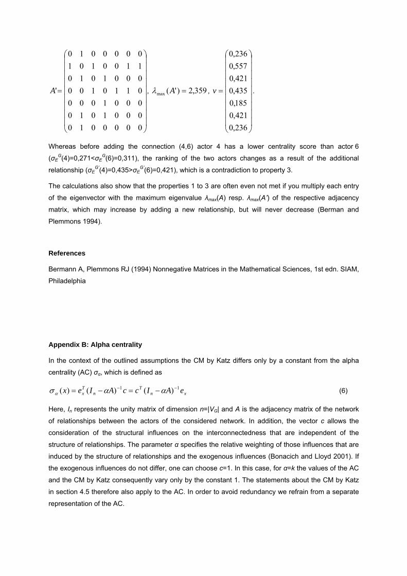
Whereas before adding the connection (4,6) actor 4 has a lower centrality score than actor 6
(σEG(4)=0,271<σE
G(6)=0,311), the ranking of the two actors changes as a result of the additional
relationship (σEG’(4)=0,435>σE
G’(6)=0,421), which is a contradiction to property 3.
The calculations also show that the properties 1 to 3 are often even not met if you multiply each entry
of the eigenvector with the maximum eigenvalue λmax(A) resp. λmax(A’) of the respective adjacency
matrix, which may increase by adding a new relationship, but will never decrease (Berman and
Plemmons 1994).
References
Bermann A, Plemmons RJ (1994) Nonnegative Matrices in the Mathematical Sciences, 1st edn. SIAM,
Philadelphia
Appendix B: Alpha centrality
In the context of the outlined assumptions the CM by Katz differs only by a constant from the alpha
centrality (AC) σα, which is defined as
xnT
nTx eAIccAIex 11 )()()( −− −=−= αασα (6)
Here, In represents the unity matrix of dimension n=|VG| and A is the adjacency matrix of the network
of relationships between the actors of the considered network. In addition, the vector c allows the
consideration of the structural influences on the interconnectedness that are independent of the
structure of relationships. The parameter α specifies the relative weighting of those influences that are
induced by the structure of relationships and the exogenous influences (Bonacich and Lloyd 2001). If
the exogenous influences do not differ, one can choose c=1. In this case, for α=k the values of the AC
and the CM by Katz consequently vary only by the constant 1. The statements about the CM by Katz
in section 4.5 therefore also apply to the AC. In order to avoid redundancy we refrain from a separate
representation of the AC.

References
Bonacich P, Lloyd P (2001) Eigenvector-like measures of centrality for asymmetric relations. Social
Networks 23(3):191-201
Appendix C: Comments on the validity of property 3 for the CM by Katz
Description of the Simulation:
The verification of whether the CM by Katz satisfies property 3 was analytically not possible in the
general case. Therefore, we simulated contiguous networks with 5 to 1000 nodes and examined the
effect of adding an edge (x,y) on the ranking of two previously not directly connected nodes x and y.
As the ranking of the newly connected nodes did not change having carried out approximately 1
million tests, we assumed that property 3 is met by the CM by Katz in general.
The networks and their modifications have been generated according to the following procedure: First,
we created a random binary matrix B. Since the adjacency matrix of the social network must be
symmetrical due to the symmetry of the relations, we mirrored the upper triangular part of the matrix B
downwards and obtain a symmetric matrix A. In a next step, all matrices which contain isolated nodes
(at least one row or column sum < 1) and thus apparently do not represent connected graphs are
rejected. For the remaining matrices we proceeded as follows: First the adjacency matrix A’ for a
modified network was calculated by identifying an entry with axy=0 and set a’xy=1 as well as a’yx=1, i.e.,
the graph received a new edge (x,y). Subsequently, we calculated the CM by Katz for both the matrix
A and matrix A’ for the nodes x and y and determined the ranking of the nodes before and after
modification of the network. Based on the described simulation study we assumed that property 3 is
satisfied when using Katz’s CM.
Partially Analytical Evidence:
For some special cases an analytical proof that property 3 is met by the CM by Katz is possible.
Therefore, we further present a formal proof of the validity of property 3 in more detail for these cases,
i.e. under certain restrictive assumptions, in the following. This consideration does not consider the
constant -1, which would be added as a result of the subtraction of the unit matrix in formula (5'),
because it is eliminated when calculating the difference in terms of the comparison of the ranking.
For the further deliberations the following denotations are used:
( ) ( )ijn akAIa =−= , ( ) ( )ijn bkAIb =−= −1 , ( ) ( )ijxy
n AkEkAIA ~~=−−=

and ( ) ( )ijxy
n BkEkAIB ~~ 1=−−=
−, with ( )xy
ijxy EE = describing the matrix whose entries – except
of the two entries xyxyE and xy
yxE – are null. The entries xyxyE and xy
yxE have the value 1 and thus
represent the added edge (x,y).
According to Sherman and Morrison (1950), by using the above denotations and applying the formula
twice to calculate the inverse of a matrix when changing one matrix entry in each case (by adding the
edge (x,y) the entries change at positions axy and ayx), we obtain the following expression:
[ ]
[ ]yyxxxyxy
xxyjxyxjxjyyixxyiyiy
yyxxxyxy
yyxxxyxyyjixxyijijyjixxyijijxyij
bbkkbkbbbkbbkkbbkbbkbb
bbkkbkbbbkbkkbbkbbkbbbkbbkbbkb
B
22
22
22
222
)1()1())((
)1()1())(())(1(~
−−−
+−+−+
+−−−
+−+−−+−−=
Hence, for ∑=
=n
iix
GK Bx
1
' ~)(σ and ∑=
=n
iiy
GK By
1
' ~)(σ it results that
[ ][ ]∑ ∑
= = −−
+−==
n
i
n
i yyxxxy
xxiyixxyix
GK bbkkb
bkbbkbBx
1 122
'
)1(
)1(~)(σ and [ ][ ]∑ ∑
= = −−
+−==
n
i
n
i yyxxxy
yyixiyxyiy
GK bbkkb
bkbbkbBy
1 122
'
)1()1(~)(σ
The difference between the centrality score of x and y in graph G‘, which results from adding the edge
(x,y), therefore is:
( ) ( ) ⎥⎦
⎤⎢⎣
⎡−−−−−
−−=Δ ∑ ∑
= =
n
i
n
iiyxxxyixyyxy
yyxxxy
G bkbkbbkbkbbbkkb 1 1
22' 11
)1(1
The denominator of this expression is abbreviated by yyxxxy bbkkbN 22)1(: −−= in the following.
Here, bxx-1≥0 holds. This can be justified by the fact that bxx-1 represents the number of paths in G
that are weighted according to their length that begin and end in x. Since this value is always positive
in a connected graph, bxx-1≥0 and thus also bxx>0 holds. Analogously, it follows that byy>0.
Property 3 comprises two statements. Sub-statement 1 refers to the ranking of two nodes that initially
have a different centrality score. The second part of property 3 makes a statement for nodes to which
the CM in the original graph assigns the same centrality score. Below, the two sub-statements are for
some special cases proven separately from each other.
Sub-statement 1)
To be shown:
)()()()( ''
11
yxbybx GK
GK
n
iiy
GK
n
iix
GK σσσσ ≥⇒=>= ∑∑
==
, i.e. 0)()( ''' ≥−=Δ yx GK
GK
G σσ

The four cases in which the first sub-statement of property 3 is satisfied in general for the CM by Katz
are outlined below:
a) Assumptions: yyxx bb > and 01 >−− xxxy kbkb
It follows from both assumptions that 01 >−− yyxy kbkb .
0)1()1( 22222 >−−>−−=⇒ xxxyyyxxxy bkkbbbkkbN
( ) ( )
[ ]{
[ ] 01111
111
0
1.00
1
1 1
'
11
>−=++−−−≥
≥⎥⎦
⎤⎢⎣
⎡−−−−−=Δ⇒
>
=>>
=
∑<∑= =
∑∑
∑ ∑==
32143421
n
iiy
Annwg
yyxx
n
iiyxxxyyyxy
bb
n
i
n
iiyxxxyixyyxy
G
bkbkbNbkbkbkbkbN
bkbkbbkbkbN N
iix
N
iiy
b) Assumptions: yyxx bb > and 01 =−− xxxy kbkb
It follows from both assumptions that 01 >=− xxxy kbkb (as k, bxx>0)
0)1()1( 22222 =−−>−−=⇒ xxxyyyxxxy bkkbbbkkbN
( ) ( ){
( )( )
011111
0
1010
1 1
' >−−=⎥⎦
⎤⎢⎣
⎡−−−−−=Δ⇒
>
==−−>>
= =∑∑ ∑321
44 344 21
n
iix
kbkb
yyxy
n
i
n
iiyxxxyixyyxy
G bkbkbNbkbkbbkbkbNxxxy
c) Assumptions: yyxx bb = and xxxy kbkb >−1
0)1()1( 22222 >−−=−−=⇒ xxxyyyxxxy bkkbbbkkbN
( ) ( ){
( ) 011111
0
1100
1 1
' >⎟⎠
⎞⎜⎝
⎛−−−=⎥
⎦
⎤⎢⎣
⎡−−−−−=Δ⇒
>
==>>
= =∑∑∑ ∑44 344 21
44 344 21
n
iiy
n
iixxxxy
n
i
n
iiyxxxyixyyxy
G bbkbkbNbkbkbbkbkbN
d) Assumptions: yyxx bb = , xxxy kbkb <−1 and xxxy kbkb <− |1|
0)1()1( 22222 <−−=−−=⇒ xxxyyyxxxy bkkbbbkkbN
( ) ( ) ( )
{( ) 011
11111
0
1100
111 1
'
>⎟⎠
⎞⎜⎝
⎛−−−=
=⎟⎠
⎞⎜⎝
⎛−−−=⎥
⎦
⎤⎢⎣
⎡−−−−−=Δ⇒
>
==<<
=== =
∑∑
∑∑∑ ∑
44 344 2144 344 21
n
iiy
n
iixxxxy
n
iiy
n
iixxxxy
n
i
n
iiyxxxyixyyxy
G
bbkbkbN
bbkbkbNbkbkbbkbkbN
In summary, the validity of the first sub-statement of property 3 can be proven for the CM by Katz, if
either (1) yyxx bb > and 01 ≥−− xxxy kbkb or (2) yyxx bb = and xxxy kbkb >−1 or alternatively
xxxy kbkb <−1 and xxxy kbkb <− |1| holds.

Sub-statement 2)
To be shown:
)()()()( ''
11
yxbybx GK
GK
n
iiy
GK
n
iix
GK σσσσ =⇒=== ∑∑
==
, i.e. 0)()( ''' =−=Δ yx GK
GK
G σσ
Assumptions: yyxx bb = and xxxy kbkb ≠− |1|
0)1()1( 22222 ≠−−=−−=⇒ xxxyyyxxxy bkkbbbkkbN
( ) ( )
( ) ( ) 01 111
111
10
1
1 1
'
=−=++−−−=
=⎥⎦
⎤⎢⎣
⎡−−−−−=Δ⇒
∑∑
∑ ∑
==
=
= =
n
iixyyxx
n
iixxxxyyyxy
n
i
n
iiyxxxyixyyxy
G
bkbkbNbkbkbkbkbN
bkbkbbkbkbN
43421
Under the conditions yyxx bb = and xxxy kbkb ≠− |1| the second sub-statement of property 3 is
satisfied when using the CM by Katz.
References
Sherman J, Morrison WJ (1950) Adjustment of an inverse matrix corresponding to a change in one
element of a given matrix. Ann. Math. Statist. 21(1):124-127