a current approach to morse and novikov theories · novikov inequalities, in quite a similar way as...
TRANSCRIPT
Universita degli Studi di Roma “La Sapienza”
Facolta di Scienze Matematiche, Fisiche e Naturali
Tesi di Dottorato
A Current Approach to Morse andNovikov Theories
Giulio Minervini
Relatore: Coordinatore del Dottorato:
Prof. Reese F. Harvey Prof. Alessandro Silva
Dottorato di Ricerca in MatematicaXIV CICLO


Introduction
The present work might be pictured in several different perspectives, accord-ing to which part of its is considered a target, which one a tool and whichan application. The results obtained are, in fact, linked to each other ina quite surprisingly strict way. The best choice to introduce and motivatethem is thus probably to describe how everything has been worked through.
The starting point is the fundamental article [13] by Harvey and Lawson,where the main results of Morse Theory on compact manifolds are retrievedin a new perspective. In particular, they construct a chain homotopy de-forming the deRham complex (of forms or of integral currents) into a finitedimensional complex of currents “the S-complex”, isomorphic to the so-called “Morse Complex”, giving a new, direct proof to the well-known factthat the latter computes the singular homology of the underlying manifold.The deformation of an object, e.g. a form α, is the asymptotic limit of thepullbacks limt φ
∗t (α) under the gradient flow of the function (convergence is
intended in the sense of currents).
A very important concept in [13] is the “finite volume technique”. Thistechnique works when one is able to bound the volume of a certain manifoldcalled the “graph of the flow”. In the case of the gradient flow of a Morsefunction, Harvey and Lawson assumed a technical hypothesis called “tame-ness” which allowed them to apply a blow up argument and desingularizethe graph of the flow, hence bounding its volume. The same hypothesis isalso assumed by Laudenbach in [17], dealing with the (a posteriori similar)problem of bounding the volume of stable manifolds in the same framework.Laudenbach too uses a blow up argument and describes the singularities ofthe stable manifolds as “conical”, conjecturing that the volume bound mightbe proved even without the “tameness” hypothesis, by “desingularizing thecone construction”. We recollect these and other preliminaries (in particularthe Boundary Value theory for systems of ODE’s) in the first chapter.
The second chapter is devoted to find bounds for the volume of the flowand of the stable manifolds of a certain class of flows with non-degenerate sin-gularities. The tameness hypothesis is removed, and the concept of “hornedstratification” is introduced to describe the singularities arisen. This model
iii

iv
turns out to be very useful and handy: horned stratified subsets define inte-gral currents, can be used as cycles for a homology theory over the integers,and at the same time have nice intersection properties. In the proofs, thetool that replaces the blow up (or “cone”) construction is the BoundaryValue theory.
In chapter three we apply the local results of the second chapter toobtain global informations. The finite volume technique is extended to anon-compact setting (a certain “weakly proper” condition is assumed inorder to compensate lack of compactedness) leading to a “non compact”Morse theory. The target is always to relate the analytic properties of aMorse function to some topological invariant of the underlying manifold.Though, of course, in a noncompact setting the results are different thanin the compact case, one might try to obtain them in somewhat the samefashion. We use the dynamics of the flow to define an analogous of the“Morse complex”, encoding the topological information. The “forward S-complex” is thus introduced, and the invariants involved are described asgroups of cohomology with “forward supports”.
Finally, the standard trick of inverting the time leads to a “forward/ba-ckward duality”, which restricts to Poincare-deRham duality if the potentialfunction is bounded. Here the proofs involve some tools by functional anal-ysis (in analogy with the proofs of deRham or Serre dualities), since thespaces might be infinite dimensional.
Once constructed a noncompact Morse theory, one looks for interestingexamples to fit in such a frame. The observation that flows arising in Novikovtheory are weakly proper suggests the attempt to relate the theories. Thisis done in chapter four.
In classical Novikov theory, cf. [22], one consider a closed 1-form withnondegenerate critical points and looks for relations between the dynam-ics of a gradient flow for the form and some topological invariant of theunderlying manifold and/or of the 1-form. Novikov, ref. cit, considered acovering of the manifold where the form is pulled back to an exact func-tion, which results of Morse type. He then introduced the “Novikov ring”and the “Novikov Complex”. The latter is made up of finitely generatedmodules over the Novikov ring, generators being in one-to-one correspon-dence with the critical points of the 1-form. This is the key to obtain theNovikov inequalities, in quite a similar way as in Morse theory one obtainsMorse inequalities. We construct a modified and arguably more naturalversion of Morse-Novikov theory, where the Novikov Ring is replaced by anew “Forward Laurent ring”. The theory results clarified in several ways.Geometrically, the Novikov complex is described as a subcomplex of thecomplex of currents, using the constructions in chapter three. Topologi-cally, the invariants are described in a new and concise way as “compact
v
forward cohomology”. A new duality called “Lambda duality” is providedfor the invariants obtained, as an application of the “forward-backward du-ality” proved in chapter three.
In chapter five, the previous results are extended to the case of functionsand forms with “Bott” singularities (i.e. singularities uniformly distributedalong regular submanifolds). The case of functions with Bott singularitieson a compact manifold using the approach by finite volume technique hadbeen considered by Latschev in his PhD thesis [18], which we generalize(and largely use!). Also, we construct a Novikov theory for forms with Bottsingularities in analogy with the approach in chapter four. Possible appli-cations and perspectives are discussed in a last section.
Finally, two appendixes are added to recollect results about currents andstratifications.
Acknowledgements
In the first place, I’d heartily like to thank my parents.I’d also like to express deep gratitude to my thesis advisor, prof. Reese
F. Harvey, and to my tutor, prof. Alessandro Silva, for their teachings, theirinterest in my work and their constant encouragement during these years.
I feel then pleased and honored to recall prof. Brendan Hasset, BlaineLawson and Piero Negrini for many useful suggestions, and prof. HariBercovici and Nicola Teleman, whose lessons deeply influenced my tasteof mathematics.
Finally, a warm greeting goes to the staff, faculty and students in MathDepartment at Rice University and to my dear friends Francesco P., Ric-cardo, Daniela, Luigi, Chun, Huey-ling, Simon, Adriano and Francesco E.,thanking the latters for some help with this thesis too.

vi
Contents
Introduction iii
1 Preliminaries 1
1.1 Morse Functions and The Morse Complex . . . . . . . . . . . 1
1.2 Finite Volume Flows . . . . . . . . . . . . . . . . . . . . . . . 3
1.3 The Boundary Value Technique . . . . . . . . . . . . . . . . . 5
2 Horned Stratifications and Volume Bounds 23
2.1 Problem and Counterexamples . . . . . . . . . . . . . . . . . 23
2.2 Horned Stratifications . . . . . . . . . . . . . . . . . . . . . . 26
2.3 Movements of Submanifolds . . . . . . . . . . . . . . . . . . . 32
2.4 Volume bound for the Flow and the Fundamental Morse Equa-tion . . . . . . . . . . . . . . . . . . . . . . . . . . . . . . . . 40
3 Non Compact Morse Theory 45
3.1 Forward Supports and the Morse Chain Homotopy . . . . . . 45
3.2 Realization of the Morse Complex . . . . . . . . . . . . . . . 49
3.3 Forward-Backward Duality . . . . . . . . . . . . . . . . . . . 52
4 Novikov Theory Revisited 55
4.1 Cyclic Coverings (Circle Valued Morse theory) . . . . . . . . 55
4.2 General Case . . . . . . . . . . . . . . . . . . . . . . . . . . . 59
4.3 Comparison with Novikov Theory . . . . . . . . . . . . . . . . 62
4.4 Lambda Duality . . . . . . . . . . . . . . . . . . . . . . . . . 65
5 Functions and 1-forms with Bott Singularities 67
5.1 The Boundary Value Technique . . . . . . . . . . . . . . . . . 67
5.2 Vector Fields and One Forms with Bott Singularities . . . . . 78
5.3 Applications and Perspectives . . . . . . . . . . . . . . . . . . 90
A Currents and Kernel Calculus 93
B Stratifications 95
vii

viii
Bibliography 99
Chapter 1
Preliminaries
In this chapter we present a brief review of the main framework we’ll workwithin and the main tool used: Morse Theory and the Finite Volume tech-nique.
A remark: we will usually don’t bother about the class of differentiabilityof our objects and will just work in the C∞ category, but of course analogousresults might be stated for less regular conditions.
1.1 Morse Functions and The Morse Complex
In the sequel, X will be a smooth manifold of dimension m, not necessarilycompact. Let f : X → R be a smooth function. A point p ∈ X is calledcritical for f if df |p = 0, i.e. all first partial derivatives of f vanish inp. It then makes sense to consider the symmetric bilinear form Hp (f) :TpM × TpM → R whose expression in a coordinate system x1, . . . , xn is
given by ∂2f∂xi∂xj . This form is called the Hessian of f in p and the critical
point p is called nondegenerate if and only if Hpf is nondegenerate. Inthis case, if the Hessian has signature (k, n − k), say, then k is called theindex of f in p and denoted by # (p). The Morse Lemma states that anyfunction with a non degenerate critical point of index k admits (locally nearp), an expression in suitable coordinates x1, . . . , xn as a quadratic form:
f (x) = f (p) + x21 + · · ·+ x2
k − x2k+1 − · · · − x
2n
Definition 1.1.1 A function whose critical points are all nondegenerate iscalled a Morse function.
It is well known that the set of Morse function is open and dense in the setof C∞ functions on a manifold.
One might define nondegenerate singularities also for vector fields, butit’s better to use a slightly less general concept. Suppose that a vector field
1
2 Chapter 1
V has an isolated singularity in a point p and that for coordinates x1, · · · , xnnear p, the expression
V (x) = Ax+ b (x)
holds, A being a constant n × n matrix (linearization matrix) and b asmooth function, vanishing and singular in p. The isolated critical point p iscalled hyperbolic if the matrix A has no purely imaginary eigenvalue (i.e.all eigenvalues have nonvanishing real part, called characteristic exponent).The number of negative characteristic exponents of the matrix A is calledthe index of the critical point p for V . Of course, the singularities of avector field V which is the gradient of a Morse function f with respect toany Riemannian metric are hyperbolic and the two notion of index agree forV = −∇f .
If V is a complete vector field, (φt)t∈Ris the corresponding flow and p is
a hyperbolic singular point of index k for V , one can introduce the StableManifold Sp and the Unstable Manifold Up in p:
Sp = x ∈ X| limt→+∞
φt (x) = p
Up = x ∈ X| limt→−∞
φt (x) = p
Theorem 1.1.2 (Hadamard) The stable and unstable manifolds at p aresmooth immersed submanifolds of X of dim respectively k = # (p) and n−k,transversal to each other.
The previous theorem is usually called “Stable manifold theorem”, anda proof will be provided later in this chapter.
Definition 1.1.3 A complete vector field with isolated hyperbolic singular-ities (and its flow) is said to be Smale if and only if for any two criticalpoints p and q, the Stable manifold at p and the Unstable manifold at qintersect transversally (of course the intersection might be empty).
We next describe the Morse complex, firsts introduced by E. Witten in[31].
Consider a compact oriented manifold X and a Morse function f : X →R with a Smale gradient. The group of k-cycles Ck is the free abelian groupgenerated by the critical points of index k, i.e. Ck ≈ Z
rk if there are rkcritical points of index k. The differentials δk : Ck → Ck−1 are defined as
δk (p) =
rk−1∑
i=1
ciqi
where ci are integers and the qi’s runs through the critical points of indexk−1. The constants ci are computed counting with orientations the numberof flow lines connecting p and qi (cf. [1] for details).
Preliminaries 3
Theorem 1.1.4 (Morse-. . .-Floer) The Morse Complex is a complex (i.e.δ2 = 0) and has homology isomorphic to the singular homology of X.
We will prove this statement later. It’s interesting to point out that thefamous strong Morse inequalities (cf. for example [21]) are a direct algebraicconsequence of this fact but we will never use them, so we won’t describethem explicitly.
1.2 Finite Volume Flows
The theory of finite volume flows was introduced by Harvey and Lawson in[13]. It is fundamental for our presentation and hence we give a short andintuitive account here, referring to the original paper for details.
Let X be a compact oriented manifold of dimension n and φt : X → Xthe flow generated by a vector field V . For some t > 0, consider the followingsubsets:
Pt = (φt(x), x)|x ∈ X and Tt = (φs(x), x)|x ∈ X, 0 ≤ s ≤ t
Of course the Pt is a smooth oriented submanifold, being the (inverted)graph of the diffeomorphism φt, whereas Tt = Φ([0, t]×X) where Φ(x, t) =(φt(x), x). The map Φ : R × X → X × X is an immersion exactly onR × (X − Z), where Z is the set of critical points for V . Supposed fixed aRiemannian metric on X:
Definition 1.2.1 The flow φ is called a finite volume flow if R+×X−Z
has finite volume with respect to the metric induce by the immersion Φ.
If X is not compact, φ is called a locally finite volume flow if for anycompact set K in X, the volume of R
+ ×K −Z is finite with respect to themetric induce by the restriction of Φ.
Note that this concept is independent by the choice of the metric and if thereare no periodic orbits it’s equivalent to ask that the immersed submanifoldΦ(R+×X −Z) has finite n+ 1-dimensional volume. In the case of periodicorbits, one has to count the volume with “multiplicity” (but so far there isno known flow of finite volume admitting a nontrivial periodic orbit on acompact manifold).
Let’s see the applications in the case of a compact X.
Denoting by ∆ the diagonal in X × X, observe that ∆ and Pt definecurrents by integration and that Tt = Φt ∗ ([0, t] ×X) defines a current bypushforward, whose boundary is dTt = ∆− Pt. One then obtains:
4 Chapter 1
Theorem 1.2.2 If φ is a finite volume flow, then both the limits
P = limt→+∞
Pt and T = limt→+∞
Tt
exists as currents and by taking the boundary of T one obtains the followingequation of currents on X ×X:
dT = ∆− P (1.1)
Remark Since the current T = Φ∗((0,+∞)×X) and (φt(x), x) = (y, φt(y))for y = φ−t(x), it follows that
T ∗ = Φ∗((−∞, 0)×X)
is also a well defined current corresponding to the pushforward of T underthe flip (x, y)→ (y, x) on X ×X.
Using the kernel calculus for currents (an account of which is presentedin the appendix), and denoting by bold letters the operators correspondingto the kernels currents, one obtains:
Corollary 1.2.3 The following limits of operators hold:
T = limt→+∞
Tt and P = limt→+∞
Pt (1.2)
as well as the equation
d T + T d = I−P (1.3)
Remark Note that T : Ek(X)→ D′k−1(X) and P : Ek(X)→ D′k(X); hereE denotes the smooth forms and D′ the currents.
By deRham theory, the operator I : Ek(X) → D′k(X) induces an iso-morphism on real cohomology. Because of the chain homotopy 1.3, so doesP:
Corollary 1.2.4 The map induced in cohomology
P : Hk(X,R)→ Hk(X,R)
is an isomorphism.
Of course the finite volume technique gains interest and power whenthere is an explicit description for the kernels T and P and a nice descrip-tion for the corresponding operators.
Preliminaries 5
If X is not compact, the situation is more complicated and locally finitevolumes flows are not always so important as in the compact case. Thecurrent equation 1.1 still makes sense, even if the condition on finite volumeis only required locally. The corresponding operator equation 1.3 continuesto hold, though it is not any longer true that I induces an isomorphism incohomology, in general.
To get additional informations out of the operator equations, we needto find a setting where I is an interesting map. This will be the case in ourtreatment of noncompact Morse theory, where the operators will be suitablyextended.
1.3 The Boundary Value Technique
We are interested in the local properties of solutions of ODE systems onRs × R
u of the form: x = L−x+ f(x, y)
y = L+y + g(x, y)(1.4)
SettingF = (f, g) : R
s × Ru → R
s × Ru
it is assumed that:
F (0, 0) = 0 and dF (0, 0) = 0
It is also assumed that L− (respectively L+) is a constant matrix whoseeigenvalues have strictly negative (respectively strictly positive) real partsand that F is smooth.
According to the Grobman-Hartman theorem, the system is topologicallyconjugated to the linear part, but no such description is available, in general,in the smooth category. Nevertheless the behaviour is “dominated” by thelinearization: basically, the flow contracts the set of x directions and expandsthe y’s.
The usual way by which one describes the geometry of a dynamical sys-tem is the Initial Value problem (abridged I.V. problem): give an initialdatum, and look for solutions as curves starting at that point for a fixedtime. This approach is very intuitive, but does not work properly in termsof stability: a slight modification of the datum can change the picture ofsolutions dramatically. The phenomenum is critical in presence of singular-ities; nevertheless, at least for hyperbolic singularities, one can describe thegeometry of the flow in a “stable” way using the Boundary Value technique.
We next give an account of this theory, quoting the book [27] and theappendix in the paper [1] as references. For what we know, the BV tech-nique was first introduced by Shilnikov in the late ’60 (cf. the introductionin [27]). Nevertheless, Shilnikov is never mentioned in the paper [1], where
6 Chapter 1
the authors refer to Smale and Floer as implicit sources.
For reasons that will be clear later, it’s better to consider a slightlymore general dynamical system than (1.4). The non linear term are sup-posed small near 0, instead of vanishing, the system non-autonomous anddepending on extra parameters:
x = L−x+ f(t, x, y, θ)
y = L+y + g(t, x, y, θ)(1.5)
The matrices L− and L+ are assumed to be in Jordan form, the realparts of the eigenvalues (i.e. the characteristic exponents) of L− to bestrictly negative, say −λs ≤ · · · ≤ −λ1 < 0, and those of L+ to be strictlypositive, say 0 < µ1 ≤ · · · ≤ µu. The Jordan form hypothesis implies thatfor any fixed value 0 < α < λ1, µ1, the following estimates hold:
∥∥∥etL−∥∥∥ ≤ e−αt ,
∥∥∥e−tL+∥∥∥ ≤ e−αt for t ≥ 0
In the sequel the symbol |x, y| will always mean the max between |x| and|y|. Now put:
F = (f, g) : R× Rs × R
u ×W → Rs × R
u
the set W (an open set in some Ri) being the domain of the parameters θ.
The “non linear term” F is supposed to vanish at the origin and its spatialderivatives to be uniformly bounded. In other words, there exists constantsδk such that:
F (t, 0, 0, θ) = 0
δkεdef= sup
|x,y|≤ε
∑
|m|≤k
∣∣∣∣∂kF
∂(x, y)m
∣∣∣∣ ≤ δk < +∞
(1.6)
We will later ask the first derivatives to be bounded by a small constant,i.e. δ1 to be small enough.
Lemma 1.3.1 In the previous hypotheses, the following inequality holds
|F (t, x, y, θ)| ≤ δ1|x,y||x, y| (1.7)
Proof. By the mean value theorem:
|F (t, x, y, θ)| = |F (t, x, y, θ)− F (t, 0, 0, θ)| ≤ δ1|x,y||x, y|¤
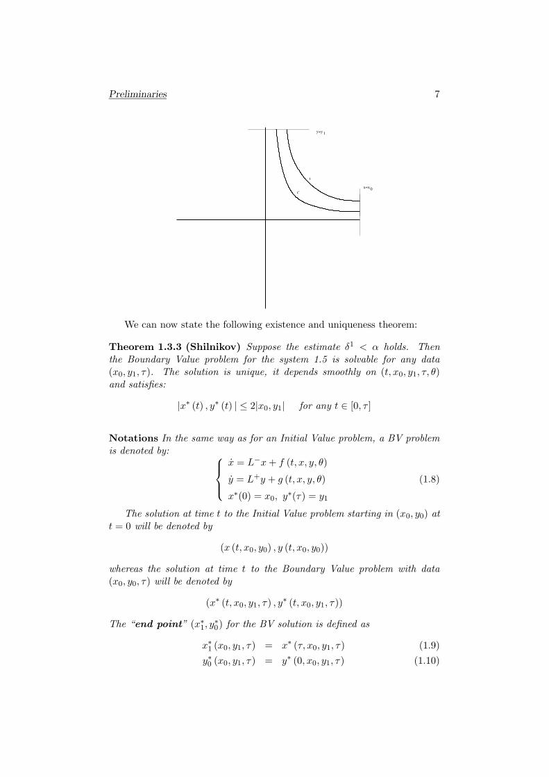
Definition 1.3.2 We say that the Boundary Value problem (abridgedB.V. problem) with data (x0, y1, τ) ∈ R
n× [0,+∞) is solvable for the system(1.5) if there exists a solution (x∗(t), y∗(t)) defined on [0, τ ] and satisfying:
(x∗(0), y∗(τ)) = (x0, y1)
Preliminaries 7
y=y1
x=x0
t
t’
We can now state the following existence and uniqueness theorem:
Theorem 1.3.3 (Shilnikov) Suppose the estimate δ1 < α holds. Thenthe Boundary Value problem for the system 1.5 is solvable for any data(x0, y1, τ). The solution is unique, it depends smoothly on (t, x0, y1, τ, θ)and satisfies:
|x∗ (t) , y∗ (t) | ≤ 2|x0, y1| for any t ∈ [0, τ ]
Notations In the same way as for an Initial Value problem, a BV problemis denoted by:
x = L−x+ f (t, x, y, θ)
y = L+y + g (t, x, y, θ)
x∗(0) = x0, y∗(τ) = y1
(1.8)
The solution at time t to the Initial Value problem starting in (x0, y0) att = 0 will be denoted by
(x (t, x0, y0) , y (t, x0, y0))
whereas the solution at time t to the Boundary Value problem with data(x0, y0, τ) will be denoted by
(x∗ (t, x0, y1, τ) , y∗ (t, x0, y1, τ))
The “end point” (x∗1, y∗0) for the BV solution is defined as
x∗1 (x0, y1, τ) = x∗ (τ, x0, y1, τ) (1.9)
y∗0 (x0, y1, τ) = y∗ (0, x0, y1, τ) (1.10)
8 Chapter 1
The following relations hold, by definition:
x (t, x0, y0) = x∗ (t, x0, y(t, x0, y0), t)y (t, x0, y0) = y∗ (t, x0, y (t, x0, y0) , t)
x∗ (t, x0, y1, τ) = x (t, x0, y∗0 (x0, y1, τ))
y∗ (t, x0, y1, τ) = y (t, x0, y∗0 (x0, y1, τ))
(1.11)
One of the major consequences of the previous theorem is that one can“invert” the unstable variables y in describing the flow of solutions: for anyfixed time τ , one can define the two manifolds
W 1τ = (x0, y0, t, x (t, x0, y0) , y (t, x0, y0)) | (x0, y0) ∈ R
n, 0 ≤ t ≤ τ
= (x0, y∗(t, x0, y1, τ), t, x
∗(t, x0, y1, τ), y1) | (x0, y1)∈Rn, 0≤ t≤τ⊂R
2n+1
W 2τ = (x0, y0, τ, x (τ, x0, y0) , y (τ, x0, y0)) | (x0, y0) ∈ R
n
= (x0, y∗0 (x0, y1, τ) , τ, x
∗1 (τ, x0, y1, ) , y1) | (x0, y1) ∈ R
n ⊂ R2n
The identities above express the fact that the submanifold W 1τ can be
smoothly parametrized as a graph over both the variables (x0, y0, t) and(x0, t, y1). Analogously, W 2
τ can be smoothly graphed over both (x0, y0) and(x0, y1). As a consequence of the formula for the derivatives in the implicitfunction theorem, then:
Corollary 1.3.4 The following matrices are invertible and
(∂y∗
∂y1|(t,x0,y1,τ)
)−1
=∂y
∂y0|(t,x0,y
∗0(x0,y1,τ))
(∂y∗0∂y1|(x0,y1,τ)
)−1
=∂y
∂y0|(τ,x0,y
∗0(x0,y1,τ))
Proof of the theorem. We’ll first prove existence and uniqueness of B.V.solutions, then their regular dependence on (t, x0, y1, θ). At this point corol-lary 1.3.4 would also be proved, since it does not involve any regularity inτ . Finally, we’ll use the corollary to prove the regular dependence on τ ,completing the proof.
As it should not be surprising, the BV system can be translated in asystem of integral equations:
x(t) = etL
−x0 +
∫ t0 e
(t−s)L−f(s, x(s), y(s), θ)ds
y(t) = e−(τ−t)L+
y1 −∫ τte(t−s)L
+
g(s, x(s), y(s), θ)ds(1.12)
Preliminaries 9
Fact 1.1 Any continuous curve, solution of the equations (1.12) is neces-sarily smooth in t and is a solution to the BV problem with data (x0, y1, τ).The viceversa is also true.
The proof of the Fact above is the same as for the standard integralformulation of an Initial Value problem. Solving the previous equations isthus equivalent to solve the Boundary Value problem.
The right hand side of equations (1.12) defines an operator on the spaceof continuous curves. Denote by Vτ the Banach space C0 ([0, τ ] ,Rn) endowedwith the sup norm ‖ ‖∞ , and define T : Vτ × R
n ×W → Vτ by:
(X(t), x0, y1, θ)→
T x (X) (t) = etL
−x0 +
∫ t0 e
(t−s)L−f(s, x(s), y(s), θ)ds
T y (X) (t)=e−(τ−t)L+
y1−∫ τte(t−s)L
+
g(s, x(s), y(s), θ)ds
The operator T can be considered as a nonlinear operator on Vτ de-pending on “spatial” parameters x0, y1 and on “nonspatial” parameters θ.Sometimes we will just use the notations T (X) for T (X,x0, y1, θ) if theparameters are understood fixed.
Claim 1.1 T is continuous (on Vτ × Rn ×W ).
This is quite obvious, and can be directly checked by estimating its varia-tions.
Claim 1.2 T is C∞ in the Vτ arguments.
Proof. The differentials dkT in the Vτ arguments are the linear operators
dkTX(X ′
1, . . . , X′k
)(t) =
∫ t0 e
(t−s)L−dkf |(s,X(s),θ) (X ′
1 (s) , . . . , X ′k (s)) ds
∫ τte(t−s)L
+
dkg|(s,X(s),θ) (X ′1 (s) , . . . , X ′
k (s)) ds
where X,X ′i ∈ Vτ , and dkf, dkg denote the differentials in the spatial direc-
tions. This can be proved by induction on k, for shortness we just prove theTaylor formula.
10 Chapter 1
∣∣∣(T (X +X ′)− T (X)− dTXX
′ − . . .− dkTX(X ′, . . . , X ′
))(t)∣∣∣
≤sup
∣∣∣∫ t0 e
(t−s)L−f(s,X+X ′)−f(s,X)−
∑ki=1d
if |(s,X(s),θ)(X′, . . . ,X ′)ds
∣∣∣∣∣∣∫ τte(t−s)L
+
g(s,X+X ′)−g(s,X)−∑k
i=1dig|(s,X(s),θ)(X
′, . . . ,X ′)ds∣∣∣
≤ sup
∫ t0 e
−α(t−s)|dk+1f |(s,Y (s),θ) (X ′, . . . , X ′) |ds
∫ τteα(t−s)|dk+1g|(s,Y (s),θ) (X ′, . . . , X ′) |ds
≤ sup
∫ t0 e
−α(t−s)δk+1‖X‖+‖X′‖
‖X′‖k+1
k+1! ds
∫ τteα(t−s)δk+1
‖X‖+‖X′‖
‖X′‖k+1
k+1! ds
≤δk+1‖X‖+‖X′‖
α(k + 1!)‖X ′‖k+1
which provides a uniform estimate. We point out that the rate of con-vergence does not depend on τ ¤
Claim 1.3 T is a contraction on Vτ . In fact ‖dT‖ <δ1
α(< 1 by hypothesis).
Proof. We can easily check dT to be a contraction:
∥∥dTXX ′ (t)∥∥ = sup
[0,τ ]
∣∣∣∫ t0 e
(t−s)L−df |(s,X(s),θ) (X ′(s)) ds
∣∣∣∣∣∣∫ τte(t−s)L
+
dg|(s,X(s),θ) (X ′(s)) ds∣∣∣
sup[0,τ ]
∫ t0 e
−α(t−s)δ1‖X‖|X ′(s)|ds
∫ τte(t−s)αδ1
‖X‖|X ′(s)|ds
≤δ1‖X‖
α
∥∥X ′∥∥
and therefore ‖dTX‖ ≤δ
α¤
By claim 1 and 2, according to the contraction lemma in Banach spaces,for any choice of spatial data (x0, y1), there exists a unique fixed point of theoperator T . This solves the existence and uniqueness issue for the boundaryvalue problem with data (x0, y1, τ).
Claim 1.4 For any fixed (x0, y1, θ), if ‖X‖∞ ≤ 2|x0, y1|, then ‖T (X)‖ ≤2|x0, y1| too.
Preliminaries 11
Proof. Suppose X(t) = (x(t), y(t)) satisfies |x(t), y(t)| ≤ 2 |x0, y1|. Then,recalling that T x and T y denote the components of T , and putting, forbrevity, δ = δ1
|x0,y1|, the estimate 1.7 implies:
|T x (X) , T y (X) (t)| = sup
|T x (x (t) , y (t))|
|T y (x (t) , y (t))|
≤ max
e−αt|x0|+∫ t0 e
−α(t−s)|f(s, x(s), y(s))|ds
e−α(τ−t)|y1|+∫ τteα(t−s)|g(s, x(s), y(s))|ds
≤ max
|x0|+ δ
∫ t0 e
−α(t−s) |x (s) , y (s)| ds
≤ |y1|+ δ∫ τteα(t−s)|x(s), y(s)|ds
≤ max
|x0|+ |x0, y1| δ
1α
|y1|+ |x0, y1| δ1α
≤ |x0, y1|
since δ1 ≤ α by hypothesis ¤
Claim 4 proves the estimate on the size of the solution in the statementof the theorem, because of the successive approximations principle (recallthat the solutions are the fixed points of the contraction T ).
Claim 1.5 The operator T : Vτ × Rn ×W → Vτ is C∞ regular.
Proof. T is affine in the spatial data (x0, y1) and so it depends smoothly onthem, together with its derivatives (which do not even depend on x0 nor ony1). As for the θ parameters, one can proceed as in claim 2, differentiatingunder the integral sign both T and its derivatives to get smoothness of themixed derivatives by induction. The theorem about differentiability afterregularity of partial derivatives proves the claim.
We can now prove the smooth dependence of the solutions of the BVproblem on the parameters (x0, y1, θ), as a consequence of the implicit func-tion theorem in Banach spaces. In fact, claim 3 implies that the derivativeof T − idVτ : Vτ × R
n ×W → Vτ in the Vτ variable is an isomorphism andtherefore the zeros of T − idVτ (i.e. the fixed points of T ) can be smoothlyparametrized over (x0, y1, θ). By the Fact 1 above, this means that the so-lutions to the BV problem depend smoothly on (x0, y1, θ), completing theproof of the theorem, but for the statement about regularity in τ . We ex-plicitly remark that corollary 1.3.4 is now proven too (cf. what said on thebeginning of the present proof).
12 Chapter 1
Claim 1.6 The solution to the BV problem depends smoothly on τ .
Proof. A formal problem arises for studying variations of τ in the previoussetting, since the Banach space on which T acts changes. It’s simpler tocheck differentiability directly. Recalling the identities 1.3.2 the issue reducesto show that y∗ (0, x0, y1, τ) is regular in τ . By the relation:
y1 = y (τ, x0, y∗0 (x0, y1, τ))
and using corollary 1.3.4 and the implicit function theorem, one gets thedesired regularity of y∗0 (x0, y1, τ) on τ (using the well-known regularity ofsolutions for Initial Value problems). This completes the proof of the lastclaim and of theorem 1.3.3 ¤
The previous theorem insured the regularity of solutions to a BV problemwith respect to any of its arguments. We will next look for the derivatives.Certainly they solve the “variational” systems of differential equation ob-tained by formal differentiation of system 1.5. It’s then enough to proveuniqueness of the solution to the variational system to identify these deriva-tives.
Let’s consider again the system 1.5 :
x = L−x+ f(t, x, y, θ)
y = L+y + g(t, x, y, θ)(1.13)
with the same hypothesis on the nonlinear terms as in theorem 1.3.3, andlet
(x∗(t, x0, y1, τ), y∗(t, x0, y1, τ))
be the solution of the BV problem with data (x0, y1, τ). For any v among∂∂x0
, ∂∂y1
, ∂∂θ
, substituting x∗, y∗ to x, y in 1.5 and differentiating with respectto v:
∂∂t
(∂x∗
∂v
)= L− ∂x∗
∂v+ ∂f
∂x∂x∗
∂v+ ∂f
∂y∂y∗
∂v
(+∂f∂θ
)
∂∂t
(∂y∗
∂v
)= L+ ∂y∗
∂v+ ∂g
∂x∂x∗
∂v+ ∂g
∂y∂y∗
∂v
(+∂f∂θ
) (1.14)
where the derivatives of the nonlinear terms are understood evaluated in(t, x∗(t), y∗(t)) and the last terms appear only if v is a nonspatial parameter.Denoting x∗, y∗ by X,Y , one gets the variational system:
∂∂tX = L−X + ∂f
∂xX + ∂f
∂yY(+∂f∂θ
)def= L−X + F (X,Y )
∂∂tY = L+Y + ∂g
∂xX + ∂g
∂yY(+∂f∂θ
)def= L+Y +G(X,Y )
(1.15)
Preliminaries 13
Observe that 1.15 has the same form as 1.5. Moreover, the estimates onthe first derivatives needed for the existence and uniqueness theorem 1.3.3
are exactly the same for the two systems, since∂F,G
∂X, Y=∂f, g
∂x, y. This means
that for any BV data (X0, Y1, τ), there exists a unique solution to the cor-responding BV problem for the system 1.15 . But we already know that∂x∗y∗
∂x0, y1, θsolve 1.15, thus it just remains to guess the values of
∂x∗
∂vin 0 and
of∂y∗
∂vin τ . Differentiating the equations 1.12 with respect to x0, y0 and θ
in 0 and τ gives:
∂x∗y∗
∂x0, y1, θ|0 =
(I 0 0
0 0 0
)
and∂x∗y∗
∂x0, y1, θ|τ =
(0 0 0
0 I 0
)
In particular, for the derivatives along “non spatial” parameters θ, theBV data to choose will just be all 0.
For the successive derivatives, one can proceed by iteration. For exam-ple, to find a certain k + 1th derivative of x∗, y∗, one writes the variationalsystem of the system obtained for the kth derivatives. The “nonlinear terms”are sums of terms of two kinds: either linear in the unknowns (having ascoefficients the first derivatives of the nonlinear terms of the original systemf, g) or not involving the unknowns at all.
Therefore, the estimate on the first derivatives needed in the existenceand uniqueness theorem is always fulfilled, as in the above case of firstderivatives. This means that any BV problem of a variational system oforder k+1 has a unique solution. Also, for derivatives of order k+1 ≥ 2, thevariables x0, y1 enter the picture as “nonspatial” parameters (the “spatial”ones being the derivatives of order k). Therefore, the desired derivativesare solutions of the BV problem of variational equations with vanishing BVdata. Referring to [28] for a more detailed discussion, we just summarizethe results in the following:
Corollary 1.3.5 Under the hypothesis of the existence and uniqueness theo-rem 1.3.3, the derivatives to the solutions to the BV problem 1.8 with respectto the spatial BV data x0, y1 and parameters θ can be found as solutions tothe BV problem whose equations are the variational equations and the BVdata are given by formal differentiation of the old ones. In particular theBV data are zero for the derivatives in θ or anyway for derivatives of orderhigher than two.
14 Chapter 1
Of course the derivatives in t for the solutions are described by thedifferential equations themselves (of the original system or of the variationalones), so we are left to look for the derivatives in τ . The implicit functiontheorem allows us to derive them by those in t and in the other variables.Recalling the relation between solutions to the I.V. problem and to the B.V.problem:
x (t, x0, y0) = x∗ (t, x0, y (τ, x0, y0) , τ) (1.16)
y (t, x0, y0) = y∗ (t, x0, y (τ, x0, y0) , τ)
and differentiating the previous w.r.to τ :
0 =∂x∗
∂y1|(t,x0,y(τ,x0,y0),τ)
∂y
∂t|(τ,x0,y0) +
∂x∗
∂τ|(t,x0,y(τ,x0,y0),τ)
0 =∂y∗
∂y1|(t,x0,y(τ,x0,y0),τ)
∂y
∂t|(τ,x0,y0) +
∂y∗
∂τ|(t,x0,y(τ,x0,y0),τ)
On the other hand, differentiating equations 1.16 in t one obtains:
∂x
∂t|(t,x0,y0) =
∂x∗
∂t|(t,x0,y(τ,x0,y0),τ)
∂y
∂t|(t,x0,y0) =
∂y∗
∂t|(t,x0,y(τ,x0,y0),τ)
Combining those and using y1 instead of y0 as a parameter (replacingthe evaluations in a coherent way), one gets the following:
Corollary 1.3.6 The derivatives of the BV solutions in τ satisfy:
∂x∗
∂τ|(t,x0,y1,τ) = −
∂x∗
∂y1|(t,x0,y1,τ)
∂y∗
∂t|(τ,x0,y1,τ) (1.17)
∂y∗
∂τ|(t,x0,y1,τ) = −
∂y∗
∂y1|(t,x0,y1,τ)
∂y∗
∂t|(τ,x0,y1,τ)
Recalling the relations 1.9 and differentiating:
Theorem 1.3.7 The first derivatives of the endpoint map satisfy:
∂x∗1∂x0, y1, θ
|(x0,y1,τ) =∂x∗
∂x0, y1, θ|(τ,x0,y1,τ) (1.18)
∂y∗0∂x0, y1, θ
|(x0,y1,τ) =∂y∗
∂x0, y1, θ|(0,x0,y1,τ) (1.19)
∂x∗1∂τ|(x0,y1,τ) =
∂x∗
∂t|(τ,x0,y1,τ) −
∂x∗
∂y1|(τ,x0,y1,τ)
∂y∗
∂t|(τ,x0,y1,τ) (1.20)
∂y∗0∂τ|(x0,y1,τ) =
∂y∗
∂τ|(0,x0,y1,τ) (1.21)
Preliminaries 15
The kth derivatives of the endpoint map are linear combinations of terms
of the form∂hx∗
∂ht, x0, y1, θ|τ,x0,y1,τ and
∂hy∗
∂ht, x0, y1, θ|0,x0,y1,τ with h ≤ k, the
coefficients being products of other derivatives of x∗ and y∗.
Remark The previous statement will be relevant in the sequel, since we’llprove some exponential estimates on the distinguished terms above, togetherwith uniform bounds for their “coefficients”.
We are now ready to prove an important consequence of the BV tech-nique: the stable manifold theorem. We will restrict the discussion to thecase we need, even if similar arguments might be worked out in the generalcase as well.
Hypothesis From now on, the system 1.5 is supposed to be autonomous(i.e. induced by a vector field).
We start extending the previous results to the case when τ = ∞. Con-sider in fact the Banach space V of bounded continuous curves defined onthe half line, endowed with the sup norm. For τ = ∞ the equations 1.12become:
x(t) = etL−x0 +
∫ t0 e
(t−s)L−f(x(s), y(s))ds
y(t) = −∫ +∞t
e(t−s)L+
g(x(s), y(s))ds(1.22)
and make still sense because of the sign of the exponentials and the estimateson the nonlinear terms. The analogous of the integral operator T introducedin the proof of theorem 1.3.3 is well defined on V and the Fact and claimsin that proof are still valid (but claim 6, which deals with regularity inτ). There is basically nothing new to prove, since all the estimates arealready done. As a consequence, for any x0 (this time this is the onlyspatial parameter involved), there exists a solution x∗(t), y∗(t) which staysbounded in the ball of radius 2|x0| for all times t ≥ 0. The map x0 → y∗(0)is smooth, and thus its graph S is a smooth submanifold of dimension s.
Lemma 1.3.8 The manifold S in invariant, i.e. the generating vector fieldis tangent to S.
Equivalently, if m ∈ S then the trajectory starting on m is contained inS.
Proof. Let (x(t), y(t)) be the trajectory trough m: by definition, it solvesthe integral equations 1.22 with datum x0. If now q = (x(t0), y(t0)) is a pointon the trajectory, a simple computation proves that (x(t−t0), y(t−t0)) solvesthe equations 1.22 with datum x(t0). That is to say, q ∈ S ¤
16 Chapter 1
Lemma 1.3.9 The integral curve of any solution which stays bounded forany t ≥ 0 is contained in S.
Proof. Let (x(t), y(t))t∈R+ be such a solution. For any τ ≥ 0, the restriction(x(t), y(t))t∈[0,τ ] solves the BV problem with data (x(0), y(τ), τ) and hencesatisfies the BV equations 1.12:
x(t) = etL
−x(0) +
∫ t0 e
(t−s)L−f(s, x(s), y(s), θ)ds
y(t) = e−(τ−t)L+
y(τ)−∫ τte(t−s)L
+
g(s, x(s), y(s), θ)ds
for any t ≤ τ . The previous equations clearly converge to 1.22 for τ →∞.This proves that (x(0), y(0)) ∈ S and the previous lemma permits to con-clude ¤
Referring to the definition in section 1, the previous lemmata prove:
Proposition 1.3.10 The manifold S is the stable manifold at the origin forsystem 1.14. It is a smooth graph over y = 0 and is invariant.
A refined version will be given later.
We now turn back to the initial (“local”) system of equations 1.4. Inthis case, all the information on the size of the nonlinear terms is containedin the fact that their differential vanishes at the origin. The global behaviorof solutions might be arbitrarily wild, but since we are interested in localquestions, one can use the standard trick of cutting off the vector field awayfrom the origin. This is meaningful provide the solutions under considera-tion do not leave the region where the system is unmodified. Translatingtheorem 1.3.3 gives the following.
Theorem 1.3.11 Suppose ε > 0 is such that the estimate δ12ε < α holds.
Then the BV problem for the system 1.4 is solvable for any data (x0, y1, τ)provide |x0, y1| < ε. The solution (x∗(t, x0, y1, τ), y
∗(t, x0, y1, τ)) is unique, itdepends smoothly on all its arguments and satisfies |x∗(t), y∗(t)| < 2|x0, y1|.
The next refines proposition 1.3.10 (cf. definition in section 1).
Theorem 1.3.12 (Stable Manifold) Let Ω be a small enough neighbor-hood of the origin in R
n. Then the stable manifold S at 0 in Ω for system1.4 is a smooth graph over y = 0 (hence a submanifold of dimension s).The unstable manifold is a smooth graph over x = 0 and the intersectionS ∩ U = 0 is transversal.
Proof. We start with the thesis of proposition 1.3.10, which is still validprovide we restrict ourselves to an Ω contained in the ball of radius ε (suf-ficiently small for the hypotheses of theorem 1.3.11 to hold). We want toshow that S is tangent to y = 0 in the origin. This is a particular case ofthe slightly more general fact:
Preliminaries 17
Lemma 1.3.13 Let R be an invariant submanifold through the origin, whichis a smooth graph over y = 0. Then R is tangent to y = 0 at the origin.
Proof. Suppose that R = (x, r(x)) for a smooth function r : Rs → R
u.Consider than the change of variables
x −→ xy −→ y − r(x)
which of course transforms R into the plane y = 0. Conjugating thesystem 1.4 by this diffeomorphism (denoting the new variables by u and v),gives the new system
u = L−u+ . . .
v = dr|0L−u+ L+v + . . .
(1.23)
where the dots denote terms which vanishes to the second order at the ori-gin. We already remarked that the plane v = 0 is the stable manifold, whichis invariant. Imposing v = 0 on y = 0 proves that dr|0 = 0 since otherwisethe term −dr|0L
−u cannot be killed by terms vanishing at the second order.But dr|0 = 0 just means that R is tangent to y = 0 in the origin. Thisproves that the stable manifold is tangent to y = 0 in 0; analogously theunstable manifold is proven tangent to x = 0 at 0, completing the proof ofthe stable manifold theorem ¤
A first, direct consequence of the previous theorem is that one can choosecoordinates such that locally near the origin the stable and unstable manifoldare the coordinate planes. The invariance of these submanifolds implies thefollowing.
Corollary 1.3.14 (Straighten Coordinates) After a smooth change ofcoordinates, the system 1.4 can be written as
x = L−x+ f(x, y)xy = L+y + g(x, y)y
(1.24)
where f and g are square matrices of smooth functions vanishing in the ori-gin and x, y are column vectors. The new coordinates are called straightencoordinates since the local stable and unstable manifolds are given by y = 0and x = 0 respectively.
Straighten coordinates are very useful. For example we can prove es-timates on the behavior of solutions in a rather simple way. Let’s startrecalling the famous Gronwall lemma.

18 Chapter 1
Lemma 1.3.15 (Gronwall) Suppose that φ : [0,+∞) → R is continuousand satisfies
φ(t) ≤ a+ b
∫ t
0φ(s)ds
for a, b ∈ R, b ≥ 0. Then the following estimate holds
φ(t) ≤ aebt
Consider the system 1.24 in straighten coordinates, and suppose theestimate δ1
2ε < α holds, where δ12ε = nmax|x,y|≤ε|f(x, y)|, |g(x, y)| (this is
just the hypothesis of theorem 1.3.3). Let
(x∗(t), y∗(t)) = (x∗(t, x0, y1, τ), y∗(t, x0, y1, τ))
denote the solution to the BV problem with data (x0, y1, τ) and put δ = δ12ε.
Theorem 1.3.16 Suppose |x0, y1| ≤ ε. Then for any τ ∈ [0,+∞) thefollowing inequalities hold:
|x∗(t, x0, y1, τ)| ≤ |x0|e
−(α−δ)t
|y∗(t, x0, y1, τ)| ≤ |y1|e(α−δ)(t−τ) (1.25)
|x∗1(x0, y1, τ)| ≤ |x0|e
−(α−δ)τ
|y∗0(x0, y1, τ)| ≤ |y1|e−(α−δ)τ (1.26)
Remark The BV formalism allows us not to mind about checking that thesolution does not leave a fixed neighborhood of the origin. In fact this isalready granted by the existence and uniqueness theorem 1.3.3. Of coursesimilar estimates hold for solutions to I.V. problems, but they are valid asfar as the trajectories stay close to the origin.
The previous corollary can be read in a coordinate free way as estimatingthe distance of trajectories from the stable and unstable manifolds.
Proof. Let’s put v(s) = y∗(τ − s) and rewrite equations 1.12 in our setting:
x(t) = etL
−x0 +
∫ t0 e
(t−s)L−f(x(s), v(τ − s))x(s)ds
v(t) = e−tL+
y1 −∫ τte(t−s)L
+
g(x(s), v(τ − s))v(τ − s)ds
Rescale the second integral to get:
x(t) = etL
−x0 +
∫ t0 e
(t−s)L−f(x(s), v(τ − s))x(s)ds
v(t) = e−tL+
y1 −∫ t0 e
−(t−s)L+
g(x(τ − s), v(s))v(s)ds(1.27)
The two equations are formally identical, so we’ll just work on the first.
Recalling that∥∥∥etL−
∥∥∥ ≤ e−tα:
Preliminaries 19
|x(t)| ≤ e−αt|x(0)|+
∫ t
0e−(t−s)αδ|x(s)|ds
Gronwall’s lemma applied to eαt|x(s)| gives the desired estimate ¤
Similar estimates also hold for the derivatives of the solution to theBV problem. It has already been observed that these derivatives can befound as solutions to BV problems of the appropriate variational systems.Unfortunately, the variational system are not any longer “straighten” withrespect to their own coordinates (and not even autonomous) and so wecannot just repeat the same argument. Still, there is a common form forall the variational systems we need. In particular any system computingthe (k)th derivatives either in t or in the spatial variables x0, y1 will havevariables Xk, Y k and an expression like:
Xk = L−Xk + f(x∗, y∗)Xk + (· · · )Xk−1 + . . .+ (· · · )x˙Y k = L+Y k + g(x∗, y∗)Y k + (· · · )Y k−1 + . . .+ (· · · )y
(1.28)
where the symbols X i stand for terms which are ith derivatives of entriesof x and similarly for Y . In this case the coefficients of each addendum X i
is a sum of k-i derivatives of the non linear terms f and g, and thereforethey can be estimated using the global bounds δh. This permits to use aninduction argument in order to estimate Xk and Y k. There is a warning.The estimates are not any longer valid within the same ball as before buton smaller ones, depending on the order of derivative; quite surprisingly,though, the size of the neighborhood depends only on estimates on the firstderivatives of f and g. Before stating the theorem, we need a refined versionof the Gronwall lemma.
Lemma 1.3.17 Suppose that φ, a, b : [0,+∞) → R are three continuousfunctions; a is nondecreasing, b nonnegative, and:
φ(t) ≤ a(t) +
∫ t
0b(s)φ(s)ds
Then the following holds:
φ(t) ≤ a(t)eR t
0b(s)ds
With same notations as in the previous theorem 1.3.16 we can state:
Theorem 1.3.18 Suppose ε > 0 is such that kδ1 < α. Let X∗(t), Y ∗(t) besome kth-order derivatives of (x∗, y∗) in the spatial variables x0, y1 and/or
20 Chapter 1
in the time variables t, τ . The following inequalities hold, for some constantCk > 0:
|X∗(t)| ≤ Cke−(α−kδ)t
|Y ∗(t)| ≤ Cke(α−kδ)(t−τ)
Proof. By corollary 1.3.6, it’s enough to mind about the case of derivativesin the spatial or t variables. We can then use the expressions 1.28. As inthe proof of theorem 1.3.16 let’s put V (s) = Y (τ − s), so that the integralequations corresponding to 1.28 become:
X(t) = etL
−X(0) +
∫ t0 e
(t−s)L−(f(x(s), v(τ − s))X(s) + . . .) ds
V (t) = e−tL+
V (0)−∫ t0 e
−(t−s)L+
(g(x(τ − s), v(s))V (s) + . . .) ds(1.29)
where we’ve already rescaled the second integral and the dots mean termsfactoring through less order derivatives of the solutions. Since the two equa-tions are of the same kind, we just give the proof for the first one. Byinduction, supposing the thesis true for 1, . . . , k − 1, one can find a Dk s.t.
|X(t)| ≤ e−αt|X(0)|+
∫ t
0e−(t−s)α
(δ|X(s)|+Dke
−(α−(k−1)δ)s)ds
≤ e−αt|X(0)|+Dk/((k − 1)δ)e−α+(k−1)δt +
∫ t
0e−(t−s)αδ|X(s)|ds
By Gronwall lemma applied to eαt|X(t)| then:
eαt|X(t)| ≤
(|X(0)|+
Dk
(k − 1)δe(k−1)δt
)eδt
from which the thesis follows readily ¤
By theorem 1.3.7, in the same hypothesis of the previous theorem, itthen follows:
Theorem 1.3.19 Let V ∗(τ) denote some derivative among∂kx∗1
∂kx0,y1,τ|(x0,y1,τ)
or among∂ky∗0
∂x0, y1, τ|(x0,y1,τ). Then the following inequality holds, for some
constant Ck > 0 not depending on x0, y1, τ :
|V ∗(τ)| ≤ Cke−(α−kδ)τ (1.30)
Conclusions We finally draw out the two consequence which will be usedin the sequel of the present work. For the sake of clearness we repeat all the
Preliminaries 21
hypothesis here.
Consider a vector field on Rn having the origin as an isolated hyperbolic
singularity (cf. definition 1.1) and let φ = (φt)t∈R be the flow of solutions.Then there exist “straighten coordinates” x, y near the origin for which thelocal stable manifold S is given by y = 0, the local unstable manifold Uby x = 0. Moreover, consider the unit ball B = (x, y)| |x, y| < 1 anddecompose its boundary in the two pieces
∂+B = |x| = 1, |y| ≤ 1 ∂−B = |x| ≤ 1, |y| = 1
We can suppose that ∂−B and ∂+B are transversal to the vector field andthat if a point m ∈ ∂+B does not belong to the stable manifold U, thenthe trajectory starting from m will touch ∂B again in ∂−B. This is grantedby corollary 1.3.14 and the estimates in theorem 1.3.16. The constructiondefines a “first escape” map
ϕ : ∂+B\S → ∂−B\U
which is clearly bijective. Since the vector field is not tangent to ∂±B andthe flow of solutions is a smooth map, an application of the implicit functiontheorem proves
Theorem 1.3.20 The first escape map
ϕ : ∂+B\S → ∂−B\U
is a diffeomorphism.
Consider now the submanifold
W = (φ t
1−t(m),m, t
)|m ∈ R
n, t ∈ (0, 1) ∩B ×B × (0, 1) ⊂ R2n+1
Theorem 1.3.21 The closure W = (W,∂W ) inside B×B×R is a smooth,closed submanifold inside with boundary:
∂W = U × S × 1 ∪∆× 0
where ∆ denotes the diagonal in B ×B.
Proof. Using the starred notation for the solution to the BV problem, bythe existence and uniqueness theorem one can reinterpret W as:
W =(φ t
1−t(x0, y0), x0, y0, t
) ∣∣ |x0, y0|<1, |φ t1−t
(x0, y0)|<1, t∈(0, 1)
=(x∗1(x0, y1, τ
1−τ
), y1, x0, y
∗0
(x0, y1, τ
1−τ
), τ) ∣∣ |x0, y1| < 1, τ ∈ (0, 1)
22 Chapter 1
The estimates in theorem 1.3.19 now partially prove the statement. In factso far we just proved that W is Ck for arbitrarily large k on a neighborhoodwhich depends on k. But W is invariant under the map
ρ(r,s) =(m′,m, t
)−→
(φr(m
′), φs(m), σr,s(t))
for any r < 0 < s, provide r + t1−t = s+ σ
1−σ .
The value σr,s(t) solving this condition is(1− t)(s− r)− t
(1− t)(s− r − 1)− tand ρ is
hence a diffeomorphism near t = 1.Therefore, if we fix (m′,m, 1) ∈ ∂W , the (local near t = 1) diffeomor-
phism ρ(r, s) maps a neighborhood of W near (m′,m, 1) to a neighborhoodof W near a point which we can suppose arbitrarily close to (0, 0, 1) bychoosing the right r, s. Since we know that W is arbitrarily smooth near(0, 0, 1), this concludes the proof ¤
Chapter 2
Horned Stratifications andVolume Bounds
We here introduce the problem of bounding the volume of the image ofa submanifold under a flow. Some pathologies are described as well as thehypotheses (Smale and Weakly Proper) needed to avoid them, and the modelfor the expected singularities, i.e. the horned stratifications, is studied indetail. The main theorem 2.3.1 is then proved and applied to show that aWeakly Proper, Smale flow has locally finite volume.
2.1 Problem and Counterexamples
Given a flow φ on X and a regular submanifold M ⊂ X of dimension m,we want to study the subset N ⊂ X obtained by moving M under the flow,i.e. the union of trajectories of φ starting on points in M . We then statethe following:
Problem To look for conditions on the flow φ and on the submanifold M sothat N has locally finite (m+1)-volume and there is a reasonable descriptionfor the boundary of N , in the sense of geometric measure theory.
One soon realizes that it’s reasonable to suppose that M contains nofixed point and that the flow has no periodic nor dense orbits in X. It isalso clear that singularities appear when N “meets” some fixed point for theflow, and the more involved the fixed point is, the more involved N mightresult. We thus assume that φ is:
- not tangent to M ;- gradient-like with respect to a function on X;- with isolated hyperbolic singularities.
23
24 Chapter 2
Still this is not enough, in general. In fact, we will next present two(counter)examples of possible bad behaviors, pointing out what is missed ineach case.
Example 1
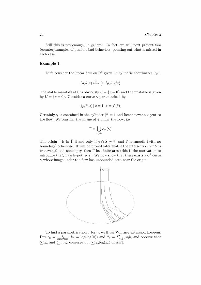
Let’s consider the linear flow on R3 given, in cylindric coordinates, by:
(ρ, θ, z)φt7−→
(e−tρ, θ, etz
)
The stable manifold at 0 is obviously S = z = 0 and the unstable is givenby U = ρ = 0. Consider a curve γ parametrized by
(ρ, θ, z) | ρ = 1, z = f (θ)
Certainly γ is contained in the cylinder |θ| = 1 and hence never tangent tothe flow. We consider the image of γ under the flow, i.e
Γ =⋃
r>0
φr (γ)
The origin 0 is in Γ if and only if γ ∩ S 6= ∅, and Γ is smooth (with noboundary) otherwise. It will be proved later that if the intersection γ ∩S istransversal and nonempty, then Γ has finite area (this is the motivation tointroduce the Smale hypothesis). We now show that there exists a C1 curveγ whose image under the flow has unbounded area near the origin.
To find a parametrization f for γ, we’ll use Whitney extension theorem.Put zn = 1
nlog2(n), bn = log(log(n)) and θn =
∑i≤n aibi and observe that∑
zn and∑znbn converge but
∑znlog(zn) doesn’t.

Volume Bounds 25
γnz
z bn n
z
z b n+1n+1
n+1
Since the “candidate slopes”
zn − 0
θn − θn−1=
1
bn→ 0
Whitney’s theorem implies that there exists a C1 function f(θ) such thatf(θn) = zn and f(1
2(θn+1−θn)) = 0. The area of the surface generated by thecorresponding curve γ is then bigger than the diverging sum
∑zn|log(zn)|,
which is the area of the image under the flow of the vertical middle segments.
Example 2
Here the problem is compactedness. Too much mass from distant pointsaccumulates in a small region. The flow is the gradient of the height func-tion on a tubular surface with some wiggles. The manifold M is a discretesequence of points and N is hence a family of flow lines. Since they accu-mulate in the lowest point, the volume of N necessarily blows up, as thepicture shows.
To avoid the pathological behaviour shown in this example, we’ll next in-troduce the Weakly Proper hypothesis.
Let φ be the flow of a complete vector field V on a manifold X. Bya broken flow line of φ we mean a piecewise smooth curve whose piecesparametrize flow lines. For points x, y ∈ X we’ll write x 4 y if there is abroken flow line connecting x and y (and x ≺ y if in addition x 6= y).
Definition 2.1.1 Let A,B ⊂ X. The set of points lying on a broken flowline starting at a point in A and ending on a point in B is called the shadowof A into B and denoted by LAB ⊂ X. In particular, the shadow of A,denoted by LA = LA∅ is the set-union of broken flow lines starting at a pointin A; similarly one defines LB, the shadow into B.
26 Chapter 2
Recall now that the vector field V is said to be gradient-like withrespect to a function f : X → R if and only if V (f) < 0 away from thecritical points of f . Of course, any gradient vector field is gradient like1
with respect to his potential function (by analogy, if V is gradient-like withrespect to f we also say that f is a weak potential for V ). We can nowintroduce the following:
Definition 2.1.2 A vector field V is said Weakly Proper with respect tof if
• V is gradient-like with respect to f
• For any compact set K contained in a slab F = f−1[a, b] then theshadows LKF and LFK are compact.
Actually, for some vector fields it’s enough to restrict the test to the casewhen K is a point, in fact:
Proposition 2.1.3 Suppose V is gradient like for f and has isolated sin-gularities. If each broken flow line contained in a slab is relatively compact,then V is weakly proper with respect to f .
Proof. For any vector field, the closure of an invariant set is an invariant set.If the vector field has isolated singularities, this implies that if a sequenceof broken flow lines has a common accumulation point, then it contains abroken flow line in its closure.¤
In the general case, sequences of flow lines might accumulate inside crit-ical sets (and so not converge to broken flow lines), and the previous state-ment doesn’t hold. Nevertheless, being isolated is not a necessary condition:a counterexample is provided by Bott singularities (cf. chapter 5), whereagain the set of broken flow lines is “weakly compact” in the sense of theprevious proof.
2.2 Horned Stratifications
We introduce the model of horned stratifications for the submanifold arisingin the problem discussed in the previous section and have a digression ontheir features. A review about stratified spaces is provided in the AppendixB.
Definition 2.2.1 A compact stratified set Y of dimension k will be calledcompact horned-stratified (or compact h-stratified) set if:
1We use this convention to be consistent with later choices.
Volume Bounds 27
• The stratification of Y is AB Whitney regular
• There exists a submersive map π : M → Y from a k-dimensionalcompact manifold with corners M to Y .
The manifold M will be called a desingularization for Y and the map π ah-projection. A locally h-stratified set Y ⊂ X is a stratified set whichlocally coincide with a compact horned stratified set.
The word “horn” comes from the typical picture of a horned stratifiedset near the zero dimensional strata. Note that M and Y have same dimen-sion.
Remark. The A-regularity requirement in the previous definition is redun-dant, being a consequence of the existence of the desingularization. It is notso for B regularity, though.
The horned stratified sets have very nice geometric properties. Let’s startwith a topological one: it helps understanding the structure of a h-stratifiedset, but we’ll never use it and thus omit the (not difficult) proof.
Lemma 2.2.2 Let Mf→ Y be a surjective map between two compact Haus-
dorff spaces. Suppose thatM is connected, f−1(
Y ) =
M and f |
M:
M →
Y
is a local homeomorphism. Then f | M
:M →
Y is a finite covering (in
particular all fibers over interior points have same cardinality).
The compactdness hypothesis was fundamental in the previous lemma,a proof of which can be found via the open-close trick.
Proposition 2.2.3 Let Mf→ Y be a desingularization of a compact h-
stratification and fij : Mi → Yj the restrictions to the strata. If the dimen-sion of Mi and Yj coincide, then fij is a finite covering.
We next analyze the behavior under intersections.
Proposition 2.2.4 Let Y ⊂ X be a h-stratified set and Z ⊂ X a closedsubmanifold. Suppose that each stratum of Y is transversal to Z. Then thefamily of all intersections of strata makes up a h-stratification for Z ∩ Y .
Proof. By proposition B.0.6, it remains to prove the desingularization part.Let f : M ⊂ N → X be a local desingularization for Y . By hypothesis, therestriction of f to any stratum of M is transversal to Z and thus M∩f−1(Z)is a compact manifold with boundary. The latter h-projects onto Y ∩Z viaf , because of the following linear-algebraic lemma ¤
28 Chapter 2
Lemma 2.2.5 Let V 1 ⊂ V 2 and W 1 ⊂ W 2 be finite dimensional vectorspaces and let L : V 2 → W 2 be a linear map. Suppose L(V 1) +W 1 = W 2
(i.e. the restriction of L to V 1 is transversal to W 1). Then V 1+L−1(W 1) =V 2 and L : V 1 ∩ L−1(W 1)→ V 1 ∩W 1 is surjective.
Corollary 2.2.6 The previous proposition holds if Z is replaced by a closedsubmanifold with corners, provide all possible intersection are transversal.
Actually, Z can be replaced by a horned stratified set too, as we nextshow.
Lemma 2.2.7 Let f : X1 → X2 be a smooth map and Mπ→ Y be a h-
stratified subset of X1. Then the graph G of the restriction f |Y , i.e.
G(f) = (y, f(y)) |y ∈ Y ⊂ X1 ×X2
is naturally a h-stratified set, the desingularization of G(f) being the graphof the map f π.
Proof. The graph G(f) is the intersection of the graph of f with Y ×X2;apply proposition 2.2.4 ¤
Proposition 2.2.8 Let f : X1 → X2 be a smooth proper map, and Y ⊂ X2
a h-stratified space. If f is transversal to Y , then f−1(Y ) is h-stratified aswell.
Proof. Let g : M ⊂ N → Y ⊂ X2 be a local the desingularization of Y andlet GM ⊂ (X2 × N) be the (inverted) graph of the restriction of g to M .Consider now, inside X1×X2×N , the closed submanifold graph(f)×N andthe submanifold with corners X1×GM . The transversality hypothesis forcesthose to be transversal, while the proper assumption makes the intersectioncompact when M is. The projection onto X1 is then a h-projection ontof−1(Y ) ¤
The previous proposition, combined with corollary 2.2.6 and lemma 2.2.5yields:
Corollary 2.2.9 Let f : X1 → X2 be a smooth map, Y ⊂ X2 a h-stratifiedspace and Z a compact manifold with corners. If f restricted to any stratumof Z is transversal to Y , then f−1(Y ) ∩ Z is horned-stratified too.
The intersection of transversal horned stratified sets is a horned stratifiedset:
Proposition 2.2.10 Let Y1, Y2 ⊂ X be h-stratified sets and suppose that allpossible intersections of strata of Y1 and Y2 are transversal. Then the familyof these intersections is a h-stratification for the set Y = Y1 ∩ Y2.
Volume Bounds 29
Proof. Since the intersection of regular stratified sets is regular (cf. propo-sition B.0.6), it’s enough to find a desingularization for Y ; we also assumeeverything to be compact. Let f, g : Mi ⊂ Ni → Yi ⊂ X for i = 1, 2be desingularizations (the domains are compact manifold with corners). Amanifold with boundary M which desingularizes Y = Y1 ∩ Y2 is the pull-back intersection: M = (p, f(p) = g(q), q)|p ∈ M1, q ∈ M2. Observe thatM1 ∩ f
−1(Y2) is a h-stratified space inside N1 (and the same property holdswith indexes interchanged), then apply the trick of the graph as in the proofof proposition 2.2.8 ¤
Corollary 2.2.11 Let Y1, Y2 ⊂ X be h-stratified sets and y ∈ Y1 ∩ Y2. Ifthe two strata containing y intersect transversally, then all the strata neary intersect transversally and hence, near y, the intersection Y1 ∩ Y2 is ah-stratified set.
Let’s now look at the metric properties of h-stratified sets.
Proposition 2.2.12 A (locally) h-Stratified set of dimension m has (lo-cally) finite m-dimensional measure.
In the previous statement, one can take as “m-measure” the Hausdorffmeasure of any Riemannian metric on the ambient space; this equals them-dimensional volume of the (union of the) top strata, which is a locallyclosed submanifold. The volume of the stratification is in fact bounded by aconstant times the volume of the desingularization. The constant dependson an upper bound for the first derivatives of the h-projection, as a conse-quence of the Area formula (cf. [10], theorem 1.2.1).
Remark Suppose that for a compact h-stratified set M ⊂ Nf→ Y ⊂ X, the
desingularizing manifold with corners M is oriented, i.e. its top stratum isoriented, so defining orientations on the codimension 1 strata (the “faces”).In this case, M defines a current of integration [M ] on N and there is awell defined pushforward current f∗[M ] on X which is obviously supportedon Y . Because of possible multiplicities, this might not coincide with thecurrent of integration on Y (assuming Y is oriented) whose existence wouldbe granted by the previous proposition.
Definition 2.2.13 A current T of dimension k on a manifold X is a fi-nite h-chain (current), or finite horned chain, if there exists a finite
number of compact h-stratifications Miπi→ Yi (with all Mi oriented) such
that T =∑
i πi ∗([Mi]). A (local) h-chain (current) is a current whichlocally coincides with a finite h-chain.
Remark The support of a h-chain does not need to be a h-stratified set, butit is a locally finite union of compact h-stratified sets. This extra structure
30 Chapter 2
of the support is relevant when dealing with intersections, as we shall seelater.
We recall that a finite chain (current) is a finite sum of currents de-fined as pushforward of standard simplexes ∆k under smooth maps, whereasa local chain (current) is a current which locally coincides with a finitechain. This terminology was introduced by deRham in [7]. Clearly theh-chain currents are chain currents and in particular integral currents (i.e.rectifiable with rectifiable boundary, cf. [8] def. 4.1.24), in fact:
Proposition-Definition 2.2.14 The current boundary dT of a (horned)chain T is again a (horned) chain current. The spaces C∗ of chain currentsand H∗ of h-chains are therefore subcomplexes of the complex of integralcurrents.
Proof. The proof is trivial for chain currents. As for horned chains, if thedesingularization T = π∗M holds on a open set U (note that π(M) is notsupposed contained in U), then the boundary dT = π∗(dM). We know thatdM is a sum of faces (since M is a manifold with corners), and each facedoes contribute (after the pushforward) to the boundary dT only if the di-mension does not decrease via the projection. The restriction of π to thesefaces are again h-projections and so dT is a local h-chain ¤
Observed that the pushforward of a chain current under a smooth propermap is again a chain current, the following is a consequence of corollary 2.2.9and proposition 2.2.10.
Proposition 2.2.15 Let [T ] be a k-dimensional horned chain current in Rn
and [S] a chain current of dimension l. Suppose that the maps which locallydefine [S] are transversal to any stratum of the stratified sets on which T issupported. Then [S] and [T ] can be “intersected” and [S] ∧ [T ] = [S ∩ T ] isa chain current of dimension h+k−n. In particular if [S] is a h-chain too,then [T ∩ S] is a h-chain.
The thesis means that for any test forms γn converging to [S] (as cur-rents), and for any β of the correct degree, the numbers T (γn∧β) converge,and the limit is [S ∩ T ](β).
Remark We will later prove, as a corollary of Morse theory, that h-chainscan be used to compute the integral cohomology of a manifold. This isdifficult to prove directly since problems arise with the “Poincare lemma”.
We instead sketch a direct proof of how the local chain currents can beused to compute the integral cohomology of a manifold. This fact is implicitin the work of deRham (cf. [7]).
Volume Bounds 31
Proposition-Definition 2.2.16 The map U → Ck(U) associating to eachopen set U in Xn the abelian group of k-dimensional chain currents on U ,with obvious restriction homomorphisms, defines a sheaf, called the sheaf of(germs of) chains of dimension k (or degree n−k). This is a subsheafof the sheaf of germs of currents.
The only thing to prove is the restriction axiom of a presheaf. If onelikes to restrict an elementary chain (i.e. a simplex) ∆ on an open set U , hecan simply present the restriction T |U (which is a current) as a locally finitesum of elementary chains in U , by triangulating the simplex in smaller andsmaller pieces. Since chains are defined to be currents with an extra localproperty, the other axioms are simple (being true for the family of currents).
The following is a trivial case of the so called “constancy theorem”, cf.[10].
Proposition 2.2.17 Let T be a 0-degree d-closed chain on the open andconnected set U . Then there exists an integer c ∈ Z such that T = c[U ].
Let’s now prove the “Poincare lemma” for chains.
Proposition 2.2.18 Let T be a d-closed chain of degree k > 0 (i.e. dimen-sion n − k < n) on the n-dimensional manifold X. Then, for any p ∈ Xthere is a neighborhood U of p and a h-chain S on U of dimension k − 1such that T |U = dS.
Proof (Cone construction). We can suppose U to be a ball in Rn. Let
M = ∪∆i ⊂ Rn′ f→ T be a (local) desingularization, with M a compact
manifold with corners (the desingularization is not assumed to be submersiveas for h-chains but it just is a sum of smooth simplexes). Consider a pointx in U and a point y close to x which is not in the support of T . For anysimplex f : ∆ → X belonging to M , let C(∆) = (t, θ)| t ∈ [0, 1], θ ∈ ∆and put
f : C(∆)→ X (t, θ)→ ty − (1− t)f(θ)
Clearly the cones f define chain currents by pushforward; by f∗(dM) =dT = 0 it then follows that f∗(C(dM)) = 0. Near any fixed x there exists ay and a small enough neighborhood V of x and y such that for any of thesimplexes ∆i partially supported on V , the cone over C(∆i) is not identicallyzero. Summing over all the simplexes ∆i, one then gets:
df∗C(M) = f∗(dC(M)) = f∗(M − C(dM)) = T
the relation dC(∆) = ∆−C(d∆) holding because the dimension of the ∆’sis not zero ¤
32 Chapter 2
The sheaves of chain currents are acyclic, in fact they are soft sheaves.Recalling that a germ T of chain current on a closed set A is the equivalenceclass of h-chains defined on a neighborhood of A under the equivalence classdetermined by coincidence on a (smaller) neighborhood of A:
Lemma 2.2.19 Let A ⊂ X be a closed set and T a germ of h-chain currenton A. Then there exists a “global” h-chain current R on X which extendsT . The sheaf of germs of h-chains of dimension k is hence soft.
Proof (Slicing). Let U be an open neighborhood of A, and R0 a chain cur-rent on U which extends T . There exist “tubular” neighborhoods V b U ofA with C∞ boundary ∂V transversal to the simplexes of R0. Transversalitycan be attained by a generic perturbation of any given regular neighborhoodof A. The intersection R = R0 ∩ V is again a chain, providing an extensionof T to all of X ¤
The previous propositions, together with a basic theorem in sheaf coho-mology proves:
Theorem 2.2.20 The sequence of sheaf maps
Z→ C0 d→ C1 d
→ · · ·d→ Cn−1 d
→ Cn → 0
is an exact resolution of the locally constant sheaf Z, and the sheaves Ck areacyclic. Hence the cohomology groups of the sheaf Z can be computed as“deRham” groups
Hk(X,Z) =T ∈ Ck | dT = 0
dR |R ∈ Ck−1
2.3 Movements of Submanifolds
All over the section (X,φ, f) will be a Weakly Proper, Smale (abridgedWPS) dynamical system.
Recall that “Weakly Proper with respect to f” means that the values ofthe “potential-like” function f strictly decrease along nontrivial trajectoriesof the flow and that the shadows of compact sets are compact within eachslab f−1([a, b]). “Smale” means that the system has isolated hyperbolic sin-gularities whose stable and unstable manifolds intersect transversally.
For each critical point, say p, we’ll assumed fixed charts Ωp in “straightencoordinates” (cf. section 1.3) such that
Ωp = (x, y) ∈ Rs ×Ru| ‖x, y‖ ≤ ε
and the stable and unstable manifold are given by
Sp = ‖x‖ ≤ ε, ‖y‖ = 0 Up = ‖x‖ = 0, ‖y‖ ≤ ε
Volume Bounds 33
The boundary of Ωp decomposes as ∂Ωp = ∂+Ωp ∪ ∂−Ωp where
∂+Ωp = ‖x‖ = ε, ‖y‖ ≤ ε ∂−Ωp = ‖x‖ ≤ ε, ‖y‖ = ε
Introducing the “link” of the stable and unstable manifold:
S+p = ‖x‖ = ε, ‖y‖ = 0 = Sp ∩ ∂
+Ωp
U−p = ‖x‖ = 0, ‖y‖ = ε = Up ∩ ∂
−Ωp
the “first escape map” provides a diffeomorphism
Θpp : ∂+Ωp\S
+p → ∂−Ωp\U
−p
We can now state the main theorem of the chapter:
Theorem 2.3.1 Let (X,φ, f) be a Weakly Proper Smale dynamical system,c ∈ R a regular value for f and M ⊂ f−1(c) a smooth (embedded) submani-fold of dimension m. Suppose M is transversal to every stable manifold andlet N =
⋃t>0
φt(M). Then the closure N coincides with the shadow LM and
is a horned stratified subset whose singular strata are unstable manifolds.
The proof of the theorem is postponed to the end of the section, but wedraw out an important consequence:
Corollary 2.3.2 The unstable manifolds of a WPS dynamical system arehorned stratified subsets whose singular strata are unstable manifolds. Thesame is true for stable manifolds (singular strata being other stable mani-folds).
Proof of the corollary For any critical point p, the unstable manifold Upis smooth near p, and its intersection with a level set f = f(p) − ε is asmooth compact submanifold, thus the theorem applies. The standard trickof reversing time proves the dual statement for stable manifolds ¤
We next prove three local results which will be the bricks in the proofof theorem 2.3.1. They describe what happens during the movement of asubmanifold respectively away from the critical points, near the first one,and near the successive ones.
The first result is just a particular case of the existence of linearizingcharts for a nonvanishing vector field and we’ll omit the proof:
Proposition 2.3.3 Let A− ⊂ f−1(b) be a closed subset and suppose LA−
f−1(a)contains no critical point, for some a < b. Then, there exist neighborhoodsU of A− in f−1(b) and V of LA
−in f−1([a, b]) and a diffeomorphism ρ :
V → U × [0, 1] which maps flow lines to “vertical” segments. In particularρ maps A− to A− × 0 and LA
−
f−1(a) to A− × [0, 1], providing an isotopy
between A− and A+ = ρ−1(A− × 1).
34 Chapter 2
For the second “brick”, let p be a critical point and Ω ⊂ Rn a straighten
chart centered in p (notations as above).
Proposition 2.3.4 Suppose A+ ⊂ ∂+Ω is a compact manifold with cornerssuch that all strata have transversal intersection with Sp. Put
A = φt(x)|x ∈ A+, t > 0 ∩ Ω
Then the closure A in Ω coincides with the shadow LA+
Ω = A ∪ Up and is acompact horned stratified set. The singular strata of A are the shadows ofthe strata in A+ and the unstable manifold Up.
The closure of A− def= A ∩ ∂−Ω is compact h-stratified too and contains
the link U+p as singular stratum.
Proof. Suppose first A+ ⊂ ∂+Ω to be a smooth, compact submanifold,transverse to Sp. Since the flow is not tangent to A+:
Fact 2.1 The parametrization
(t,m) ∈ [0,+∞)×A+ σ7−→ φt(m) ∈ A
is regular, i.e. it is a diffeomorphism.
Consider now the following submanifold of Rn × R
n × R:
W =
(x1, y1, x0, y0, t) |
0 < t < 1, |x0, y0, x1, y1| < ε(x1, y1) = φ t
1−t(x0, y0)
By the BV technique (cf. theorem 1.3.21), the manifold W is smooth inΩ× Ω× R with boundary
∂W = (0, y1, x0, 0, 1)| |x0, y1| < ε ∪ (m,m, 0)|m ∈ Ω
Define two subsets of Rn × R
n × R by:
Zdef= R
n ×A+ × R
(A1, ∂A1)def= Z ∩ (W,∂W ) =
(m′,m, t)| 0 ≤ t≤ 1,m∈A+,m′ = φ t
1−t(m)
It clearly is∂A1 = Up × (A+ ∩ Sp)× 1 ∪ ∆A+ × 0
The submanifold Z is transverse to ∂W since A+ is transverse to Sp.Away from ∂W , any intersection of the form W ∩R
n × pt is transversal, inparticular W ∩Z. Therefore, (A1, ∂A1) is a smooth compact manifold withboundary and, projecting onto the first factor via
π : Rn × R
n × R→ Rn
Volume Bounds 35
it’s π(A1)
= A and the topological boundary of A is hence Up = π(∂A1
).
The restriction of π is clearly a submersion on the singular stratum ∂A1.On the other hand, the open top stratum of A1 can be regularly parametrizedby the map σ by Fact 2.1. Also, σ factors trough π|A1 , by the definitionof W as a graph and so the restriction of π to the top stratum in A1 is adiffeomorphism too. Summarizing, the restriction
π|(A1,∂A1) : (A1, ∂A1)→ (A,Up)
is a h-projection over the stratified space A = A ∪ Up. To show that Ais horned we are left to prove the AB Whitney regularity conditions for astratification. It’s actually enough to prove B, thanks to the remark afterdefinition 2.2.1. But B-regularity is equivalent to prove that the normalspheres in any small C1 tubular neighborhood of the singular stratum Upare transversal to A (see theorem B.0.5 in the appendix). This is triviallytrue because A is a union of flow lines, which are already transversal to thosespheres.
Finally, the intersection (A−, U−p ) = (A,Up) ∩ ∂
−Ωp is transversal, and
so the closure A− is h-stratified too, by proposition 2.2.4.
All the previous arguments still hold with obvious modifications if A− isreplaced by a manifold with corners transversal to the stable manifold (inthe sense that any stratum is transversal to the stable manifold). The onlyreally “singular” stratum is now the unstable manifold Up: the other strataare just the shadows of the strata in A+, and their singularities are thoseof a manifold with corners, as one can prove locally using proposition 2.3.3 ¤
We can now state and prove the third “brick”:
Proposition 2.3.5 The previous proposition 2.3.4 holds word for word byreplacing “compact manifold with corners” with “compact h-stratified set”.
Proof. Let A+ be a compact submanifold with boundary which desingular-izes the h-stratified space A+. It is not restrictive to suppose A+ ⊂ R
j×∂+Ωand the h-projection to be the restriction of the projection onto the secondfactor.
Introduce now the auxiliary flow ψ on Rj×R
n by extending φ via a linearcontraction in the R
j components. In other words, ψt(x′, x) = (e−tx′, φt(x))
and the following diagram commutes
Rj × R
n ψt−→ R
j × Rn
↓ π ↓ π
Rn φt
−→ Rn
(2.1)
36 Chapter 2
The origin is a hyperbolic isolated singularity for the flow ψ; its stablemanifold is R
j×Sp and the unstable manifold is 0×Up. Clearly the stablemanifold “upstairs” is transversal to the desingularization A+ ⊂ R
j × ∂+Ω,which is a compact manifold with corners. The hypothesis of proposition2.3.4 are fulfilled for the flow ψ by the “incoming link” A+ and therefore,putting
A =⋃
t>0
ψt(A+)
the closure A (which is the shadow of A+) is a compact h-stratified setcontaining the unstable manifold Up × 0 as singular stratum.
Let’s now look to the closure A “downstairs”. Since the diagram 2.1commutes, it follows that A = π(A) and hence A = LA
+
Ω = A ∪ Up. Therestriction of π on the singular stratum 0 ×Up is a trivial projection overUp. Besides those, the other strata in A and A are respectively the shadowsof the strata in A+ and A+. It readily comes out that the projection πrestricts to be a submersion on any stratum.
To conclude that the A is h-stratified, we are left to check B-regularity(A-regularity following by the existence of the h-projection). Besides thestratum Up, the regularity conditions for the other strata can be checkedlocally by applying proposition 2.3.3. On the other hand, condition B forUp is a trivial consequence of the invariance of A (cf. the analogous argumentin the proof of proposition 2.3.4).
Finally, the intersection (A,Up) ∩ ∂−Ω is transversal and hence a com-
pact h-stratified set too ¤
We are now ready to prove theorem 2.3.1. Let’s describe its idea, whichconsists of two steps.
First, given any broken flow line γ starting on M , we’ll show that γbelongs to N and that there is a subset Ω(γ) ⊂ N containing γ which is ah-stratified space and satisfies the thesis of the theorem.
Second, we’ll show that N can be stratified arranging a locally finitefamily of these h-stratified subsets in such a way that the top strata don’toverlap. This would complete the proof.
More precisely, in the first step we define Ω(γ) by cutting the shadowLM along γ into “pipes” and “pants”. The pipes are parts not containingany critical point, and can be described using proposition 2.3.3. The pantsare parts containing a single critical point and propositions 2.3.4 and 2.3.5will be invoked.
Each pipe and pant has two distinguished components in the boundary:the “incoming link” and the “outgoing link”. For example, in the nota-tions of proposition 2.3.3, the shadow LA
−∩ f−1[a, b] is a pipe, its incoming
Volume Bounds 37
link is A− ≈ A− × 0 and its outgoing link is LA−∩ f−1(a) ≈ A− × 1. On
the other hand, in the terminology of proposition 2.3.4, the set A is a pant,A+ is its incoming link and A− ∪ U− its outgoing link. Note that new sin-gularities arise only within pants.
Proof of the theorem. Step 1.
Choose a broken flow line γ starting on M and let p1, . . . , pr be thecritical points on γ so that the flow line can be decomposed in
γ = (γ0, γ1, ..., γk) piγi→ pi+1
connecting the points x0 ∈M , p1, ..., pk (x0 is not critical but the pi’s are);observe that each γi is contained in Spi+1
(and in Upiif i 6= 0). For each pi it
is assumed chosen a chart Ωpiin straighten coordinates and the intersections
of its boundary with the flow line γ are denoted by:
xi = γ ∩ ∂+Ωpiyi = γ ∩ ∂−Ωpi
We next show how to cut off the pipes along the flow lines γi and the pantsnear the critical points pi.
Let’s start with the first pipe, along γ0, recalling that M is a closed sub-manifold of the regular level set f−1(c), and any stable manifold is transver-sal to M .
Choose a closed ball B inside f−1(c), centered in x0 and small enoughso that B “flows” inside Ωp1 , i.e. so that the all the flow lines starting onB meet Ωp1 without breaks. Since the stable manifold Sp1 is closed nearx0 (the flow line γ not being broken up to p1), Sp1 intersect transversallyM ∩ ∂B, provide B is small enough.
Moreover, since the flow has no fixed points on the shadow LM∩B∂−Ωp1
,
proposition 2.3.3 provides a diffeomorphism LM∩B∂−Ωp1
≈ M∩B×[0, 1] obtained
by trivializing the trajectories.This shadow is the first pipe: it is a smooth manifold with corners,
the incoming link is M ∩ B and the outgoing link A+1 (corresponding to
M ∩ B × 1 via the trivializing diffeomorphism) is a submanifold withboundary contained in ∂+Ωp1 and transversal to Sp1 .
The outgoing link A+1 of the pipe above coincides with the incoming link
of the next pant, near p1, which we denote by A1. This pant is just the
shadow of A+1 into Ωp1 , i.e. A1 = L
A+
1
Ωp1
.
Since A+1 is a submanifold with boundary transversal to Sp1 , we can ap-
ply proposition 2.3.4 to desingularize the pant A1 and to find its outgoing
38 Chapter 2
link: it follows that A1 is a h-stratified set containing Up1 as singular stra-tum. The outgoing link A−
1 = A1 ∩ ∂−Ωp1 is h-stratified too and contains
the link U−p1
of the unstable manifold as singular stratum.Differing from the connection pipe-pant, the incoming link for the successivepipe will not be all the outgoing link A−
1 of the present pant, but just a smallportion of it, cut near γ.
We now proceed by finite induction to construct the pipes and pantsalong γ. Suppose constructed the pipes along γ1, . . . , γi−2 and the pantsnear p1, . . . , pi−1 (this implies that the shadow of M has been desingular-ized near γ up to pi−1). The only inductive hypothesis we need to keep trackof is that the outgoing link A−
i−1 of the last pant is a h-stratified set con-taining the link of the unstable manifold U−
pi−1= Upi−1
∩ ∂−Ωp1 as singularstratum.
The next critical point is pi, joined to pi−1 by the unbroken flow line γi−1.The stable manifold Spi
contains γi−1 and is closed near xi−1 = γ∩∂−Ωpi−1.
If B is a small ball in ∂−Ωpi−1centered in xi−1, then (B, ∂B) and A−
i−1
intersect transversally; in particular their intersection is a h-stratificationand contains a neighborhood of xi−1 inside U−
pi−1. This last fact and corollary
2.2.11 imply that, if B is small enough, then all the strata in (B, ∂B)∩A−i−1
are transversal to Spi, since U−
pi−1is. Finally, by possibly further shrinking
B, we can also assume that B∩A−i−1 “flows” into Ωpi
without meeting othercritical points.
Choosing such a ball B, the next pipe can be defined as the shadow
LB∩A−
i−1
∂+Ωpi
, which is h-stratified as a trivial consequence of proposition 2.3.3.
The outgoing link A+i = L
B∩A−i−1
∂+Ωpi
∩ ∂+Ωpiis a h-stratified space transversal
to the stable manifold Spi. Note that A+
i will be the incoming link for thenext pant, as always at the connection pipe-pant.
The pipe near pi, denoted by Ai, is the shadow LA+
i
Ωpi. To complete step
one, we apply proposition 2.3.5 to the incoming link A+i . It comes out that
the pant Ai is h-stratified and contains the unstable manifold Upias singular
stratum. Moreover, the intersection with ∂−Ωpiis transversal and hence the
outgoing link of the pant Ai is a h-stratified space containing the link U−pi
of the unstable manifold as singular stratum. This completes the inductivestep and proves Step 1.
Step 2.
So far, we desingularized the shadow LM along each compact broken flowline γ; it remains to prove that these desingularizations can be arranged into
Volume Bounds 39
a locally finite family without overlappings on the top dimensional strata.
Fix any compact set K and any b < c (recall M ⊂ f−1(c)). Because ofthe Weakly Proper hypothesis, the shadow LK
f−1(b) is compact, and hence itcontains a finite number of critical points.
The set K can be covered by a finite family of small balls Bj in M whosetop dimensional strata do not overlap (these balls are compact manifold withcorners of the same dimension of M). Also, for any j we can assume thateither Bj is disjoint by all the stable manifolds of the critical points in LK
f−1(b)
or there is one of these critical points, say p, such that Bi flows into ∂+Ωp
without meeting any other critical point.In the first case, the shadow LB
f−1(b) is a pipe. In the second case, the
shadow LB can be decomposed in a pipe up to Ωp, a pant near p and there-after we can decompose the outgoing link (which is a compact stratified setcontained in ∂−Ωpi
) cutting it by a finite number of balls, as done for Mnear K. Proceeding by finite induction using Step 1, one constructs thedesired stratification, completing the proof of Step 2.
Summarizing, we proved that the closure of N =⋃t>0
φt(M) is just the
shadow LM , it is a stratified set whose singular strata are unstable manifoldsand we showed, by passing to a refinement, that the stratification is horned;the proof of the theorem is complete ¤
As a byproduct of the previous proof, we can describe the current bound-ary on N .
Suppose X is oriented. For any critical point p choose an arbitraryorientation to the stable manifold Up so that an orientation is induced onSp by requiring that < X >=< Up > + < Sp >. Suppose finally M isoriented too and orient N by < N >=< M > + < L >, where < L > isthe direction of the flow. Observe that Up, Sp, M and N all define hornedchain currents. In particular, if M has dimension k, then the current [N ] hasdimension k + 1 and, since the singular strata of N are unstable manifolds,d[N ] is a sum with integer coefficients of unstable manifolds of critical pointsof index n− k (by dimension restrictions). We now sketch how to computethis coefficients, referring to [13] for more details.
The Smale and Weakly Proper hypothesis imply that the set of pointsin M joined to a critical point p of index n − k is finite, the intersectionSp ∩M being discrete and compact. Hence, for any p of index n − k thereis a finite number of flow lines γ from M to p.
For each of these γ, the previous proof implies that the h-projectiondesingularizing dN is a diffeomorphism onto the stratum Up. This meansthat the contribution of “γ” to the boundary of N is just ±[Up], the correct
40 Chapter 2
sign being determined by the orientations.
Corollary 2.3.6 In the notations of the previous theorem, suppose X, Mand all the stable and unstable manifolds are oriented (in such a way that< X >=< Sp > + < Up > at each critical point p). Then [M ] and [N ] arehorned chain currents and
∂ [N ] = [M ]−∑
cq[Uq]
The sum goes trough all the critical points q of index n−dimM and for anysuch q, the coefficient cq “counts with orientation” the number of flow linesjoining M and q.
Of course a similar statement holds for backward shadows, by replacingunstable manifolds by stable manifolds. In particular, for any critical pointp, the current boundary of the stable manifold Sp is given by:
∂ [Sp] =∑
cpq [Sq]
Important Remark If the manifold is compact, the coefficients cpq in theprevious formula are exactly the same we described in the construction of theMorse Complex in section 1.1. This implies that replacing a critical point byits stable manifold provides a “geometric” realization of the Morse Complexas a subcomplex of the complex of currents (interpreting the boundary inthe Morse complex as the boundary of currents).
This embedding of the Morse Complex suggests a way to define a gen-eralized Morse complex in a noncompact setting. This will be the subjectof the next chapter.
2.4 Volume bound for the Flow and the Funda-mental Morse Equation
The aim of this section is to use theorem 2.3.1 to find a bound for the volumeof a Weakly Proper, Smale flow.
We need to prove that the submanifold T ⊂ X×X defined in section 1.2(the graph of the flow) has locally finite volume. We actually show muchmore: T is a horned stratified set and its current boundary will be described.
Consider the height function h on the circle S1 and put:
H : S1 ×X ×X → R
H(θ, x, y) = h(θ)− f(x) + f(y)
Volume Bounds 41
The flow Ψ on S1 ×X ×X given by:
Ψt(s, x, y) =
(e−ts, φt(x), φ−t(y)
)for s coordinate near S
(ets, φt(x), φ−t(y)) for s coordinate near N
is gradient like with respect to H (here S and N are the South and Northpole of S1).
Lemma 2.4.1 The dynamical system (S1×X×X,Ψ, H) is Weakly Properand Smale.
Proof. The critical points of Ψ are of the kind (S, p, q) and (N, p, q), forp and q critical points of φ, and the corresponding stable and unstablemanifolds at such points are:
S(S,p,q) = S1 × Sp × Uq S(N,p,q) = N × Sp × Uq
U(S,p,q) = S × Up × Sq U(N,p,q) = S1 × Up × Sq
Clearly all possible intersection are transversal, thus insuring the Smalehypothesis. It remains to prove the Weakly Proper condition. By contradic-tion, let γ be a non compact flow line for Ψ contained in a slab H−1[a, b]; it isnot restrictive to choose γ unbroken. Since the first coordinate is bounded,the lack of compactedness comes from the x or y variable. But the con-tribute by x and y to H are of the same sign (either for positive times orfor negative ones) and so the weakly proper hypothesis for φ on X impliesthe same hypothesis for Ψ ¤
Let now 1 ∈ S1 be the point whose coordinate in the chart containingthe south pole is 1 and consider the subset
T = (e−t, φt(x), φ−t(x))| t ≥ 0, x ∈ X ⊂ S1 ×X ×X
Observe thatT =
⋃
t≥0
Ψt(1 ×∆)
and that 1 ×∆ is contained in the level set of 1/2, which we can supposeto be regular for H (if not, start from another point in S1).
Lemma 2.4.2 The submanifold 1×∆ is transversal to all the stable man-ifolds.
Proof. First observe that T does not intersect any stable manifold of thecritical points (N, p, q). The remaining stable manifolds are of the formS1 × Sp × Uq and transversality for Sp × Uq ∩ ∆ is exactly the same thentransversality of Sp ∩ Uq in X, the Smale hypothesis proves the lemma ¤
42 Chapter 2
Proposition 2.4.3 The closure of the submanifold T is a horned stratifiedset with singular strata 1 × ∆ and U(S,p,q) for any critical points q 4 p.The boundary of the corresponding chain current [T ] is:
∂[T ] = 1 ×∆−∑
[U(S,p,p)] (2.2)
Proof. The previous lemma and theorem 2.3.1 proves the first statement.on the other hand, the boundary value technique implies that, near each(S, p, p), the set T is a manifold with boundary given by 1 ×∆ ∪ S ×Up × Sq (cf. theorem 1.3.21), so the equation in the statement holds nearpoints (S, p, p) (recall S is just the south pole in the circle S1).
The current T is a horned chain and its boundary is thus a sum of sin-gular strata. By dimension restrictions, the only admissible ones are exactly1×∆ and U(S,p,p), thanks to corollary 2.3.6. Since the equation holds near(S, p, p), it then holds everywhere. ¤
We can now state the main theorem:
Theorem 2.4.4 A Weakly Proper Smale flow has locally finite volume. Infact the closure of the “total graph” T is a horned stratified set whose singularstrata are ∆ and Up × Sq for any critical points q 4 p.
The following “Fundamental Morse Equation” of h-chain currentsholds in X ×X:
dT = ∆− P (FME)
where (denoting by Cr the set of critical points)
P =∑
p∈Cr
[Up × Sp] (2.3)
Proof. Continuing with the previous notations, the projection onto thesecond factor π : S1×X×X → X×X maps T onto the “total flow” T . Theprojection is a diffeomorphism on the top dimensional stratum of T , and atrivial submersion on the singular strata 1×∆ and U(S,p,q) = S×Up×Sq(here S is just the south pole in the circle and q 4 p).
Since π is proper and T is h-stratified, to prove that T is h-stratified tooit remains to show the A-B regularity. By the remark after definition 2.2.1it’s enough to prove “B”. This is trivial along the stratum ∆ (the singularityis smooth here). Along the other strata Up × Sq, the argument is similar tothe corresponding one in the proof of theorem 2.3.1, by using the fact thatT is made up of flow lines for the (auxiliary) flow (φt, φ−t) on X ×X. Notethat ∆ is not contained in a regular level set for this auxiliary flow, that’swhy we needed to introduce T .
It’s thus proved that T is horned stratified too and the correspondingh-chain current is just T = π∗T . The equations in the statement then follow
Volume Bounds 43
by pushforwarding the relation 2.2 ¤
We end this section by applying the “locally finite volume” technique tothe previous equation. Using the kernel calculus, let
T, I, P : E∗cpt (Y ) −→ D′∗ (Y )
be the operators whose kernels are T,∆ and P (recall E denotes smoothforms and D′ currents).
Proposition 2.4.5 For any Weakly Proper, Smale dynamical system (X,φ),and any test form α on X, the limit and the integral:
P(α) = limt→+∞
φ∗t (α) =∑
p∈Cr
(∫
Up
α
)[Sp] , T(α) =
∫
R+
φ∗t (α) (2.4)
converge as currents and the following equation holds:
d(T(α)) + T(dα) = α−P(α) (2.5)
Proof. The only nontrivial fact is the integral expression for T. Since thecurrent T = Φ∗(R
+ ×X), where Φ(t, x) = (φt(x), x), for any forms α and βon X it is:
T (α⊗ β) =
∫
R+×XΦ∗(α ∧ β) =
∫
R+×Xφ∗t (α) ∧ β =
∫
X
(∫
R+
φ∗t (α)
)∧ β
and this proves the expression 2.4 for T. Note that the current T(α) isclearly smooth away from the stable manifolds of critical points in the back-ward shadow of the support of α ¤
Remark As observed in section 1.2 about the finite volume technique, equa-tion 2.5 is not so relevant if X is not compact. In fact, it provides a chainhomotopy between I and P but I does not induce any algebraically interest-ing map in topology, hence P doesn’t as well. Nevertheless, one can extendthe operators involved to act on spaces where this equation regains power.This will be done in the next section by introducing the “forward supports”.

44 Chapter 2
Chapter 3
Non Compact Morse Theory
In this chapter, starting from the Fundamental Morse Equation proved inthe last chapter, we’ll derive an equation of operators called the Morse ChainHomotopy. As the name suggests, the new equation provides a chain homo-topy between a complex of forms with some restriction on the support and anon compact analogous of the Morse complex. A noncompact Morse theoryis established, relating the dynamics of a Smale, Weakly Proper flow to thespaces of cohomology with “forward supports” of the manifold. Those are of-ten infinite dimensional and endowed with a natural locally convex topology.The standard trick of inverting the flow leads to a forward-backward duality.
All over the chapter we assume that X is an oriented n-dimensionalmanifold, endowed with a Weakly Proper, Smale dynamical system (φ, f).An arbitrary orientation is assumed chosen for the unstable manifold of eachcritical point, inducing an orientation on the stable manifolds in such a waythat < X >=< Sp > + < Up > at each critical point p.
3.1 Forward Supports and the Morse Chain Ho-motopy
We here study the operators P and T introduced in the last chapter. Thestructure and position of the stable and unstable manifolds and the expres-sions 2.4 suggests that P and T extend to forms which are supported inf−1[a,+∞) for some a ∈ R and it’s quite obvious that the range of theoperator consists of currents supported in the same way. This justifies thefollowing definition.
Definition 3.1.1 A closed set A ⊂ X is a compact/forward set (abbre-viated c/f set) with respect to the function f if both
• A∩ f−1 ([b, c]) is compact for any b ≤ c ∈ R (i.e. A is slab compact)
45
46 Chapter 3
• A ⊂ f−1 ([a,+∞)) for some constant a ∈ R (i.e. A is forward).
One can defined backward and compact/backward sets in a similarmanner. Of course, a closed set is forward (resp. backward) if and onlyif it has compact intersection with all the compact/backward (resp. com-pact/forward) sets.
Remark (stability) Suppose f0 and f1 are two weakly proper functions onX whose difference is bounded (say by the constant c ≥ 0). Then f0 and f1
determine the same family of compact/forward sets.
Since f−11 ([−∞, a)) ⊂ f−1
0 ([−∞, a+ c)) for any a ∈ R, if A is c/f withrespect to f0 then A is also c/f with respect to f1. Actually, both the notionsforward set and slab compact (cf definition of c/f set) are the same for f0
and f1.
The subscript ↑ will denote the family of forward sets while c ↑ or c/fwill denote the compact/forward ones; analogously for backward sets. Forexample, E∗↑ (X) = Γ↑(X, E
∗) and E∗c↑ (X) = Γc↑(X, E∗) denote the space of
smooth forms with forward and compact/backward support, respectively.
Clearly either of the forward, backward, c/f and c/b family of sets is aparacompactifying family for X in the terminology of Godement ([G]). Itmakes thus sense to compute (sheaf) cohomology with supports in such fam-ilies of sets. For example, one can compute the cohomology of X with realcoefficients (i.e. the cohomology of the locally constant sheaf R) and forwardsupports via deRham theorem, using either smooth forms or currents as:
Hk↑ (X,R) ≈
ω ∈ Ek↑ (X) | dω = 0
dη | η ∈ Ek−1↑ (X)
≈θ ∈ D′k
↑ (X) | dθ = 0
dρ | ρ ∈ D′k−1↑ (X)
Note that the stable manifolds have compact/forward support, whereasthe unstable manifolds are compact/backward (“compact” because of theWeakly Proper hypothesis).
As one expects, the following duality hold:
Proposition 3.1.2 The currents with compact/forward support are the con-tinuous linear functionals on the space of forms with backward support,and similarly the forward-supported currents are functionals over the com-pact/backward forms:
(Ek↓ (X)
)′= D′k
c↑ (X)(Ekc↓ (X)
)′= D′k
↑ (X)
Morse Theory 47
Proof. We just prove the first statement. For j = 1, 2 . . . the closed sets Bj=f−1(−∞, j] form an exhaustive sequence of backward sets. Now each E ∗Bj
(X)
(the space of forms with support contained in Bj) is a closed subspace ofthe Frechet space E∗ (X). Therefore
E∗↓ (X) = lim−−−−−→j→+∞
E∗Bj(X)
is the strict inductive limit of Frechet spaces (in particular, an LF-space).Since the inclusion map Ekcpt (X) → Ek↓ (X) is continuous with dense
range, the adjoint map Ek↓ (X)′ → D′k (X) is similar (i.e. 1-1, continuous,
with dense range). In particular each continuous linear functional on Ek↓ (X)
is a current. Now if T ∈ Ek↓ (X)′ ⊂ D′k (X) and spt(T ) ∩Bj is not compact(for some j), there exist a sequence of pairwise disjoint open balls Un ⊂ Bjwhose centers don’t accumulate. Pick ϕn ∈ E
kcpt (Un) with T (ϕn) = 1. Since
ϕ =∑ϕn ∈ E
k↓ (X) but T (ϕ) is not defined this is a contradiction, proving
that sptT is compact forward.Conversely, if T ∈ D′k
c↑ (X) has c/f support then T (ϕ) is defined for all
ϕ ∈ Ek↓ (X), since spt(T )∩spt(ϕ) is compact. Also, the maps T : EkBj(X)→
R are continuous. That is, D′kc↑ (X) ⊂ Ek↓ (X)′ ¤
We now turn back to the kernel currents T, ∆, P and their associatedoperators T, I and P. Let’s introduce a terminology which will only appearin the next lemma: a set A × B ⊂ X ×X will be said “compact/forward-backward” (abridged cf-b) if A is compact forward and B is backward in Xand analogously one defines “forward-compact/backward” product sets.
Lemma 3.1.3 The support of T,∆ and P has compact intersection withany product subset of X×X which is compact/forward-backward or forward-compact/backward and hence the three currents act on any form with suchsupport.
Proof. It suffices to prove the statement for T , since the supports of P and∆ are contained in sptT . Let A be forward and B compact/backward in X.Choose a sequence (xn, yn) ∈ (A×B)∩ spt(T ) and suppose that (xn, yn)doesn’t accumulate. The points xn ≥ yn lie on the same (broken) flow line.There are two cases:- If the yn don’t accumulate, then necessarily f(yn) is not bounded below(since B is c/b) and therefore also f(xn) ≤ f(yn) is unbounded below, whichcontradicts xn to be a forward set.- If the yn accumulate in y, it’s f(xn) ≤ f(y) + ε and hence the points xnlie in some slab f−1[−a, f(y) + ε], since A is forward. The weakly properhypothesis then implies that the points xn necessarily accumulate since theyn do. An analogous argument proves the c/f-c case ¤

48 Chapter 3
By the very construction of the operator associated to a kernel current,the previous lemma, together with proposition 2.4.5 proves the next theo-rem:
Theorem 3.1.4 The operators T, I and P associated to the kernel currentsT , ∆ and P , which a priori are operators from
E∗cpt (X) −→ D′∗ (X)
extend to continuous operators from
E∗↑ (X) −→ D′∗↑ (X)
and satisfy the following equation, which we call Morse Chain Homotopy:
d T + T d = I−P (3.1)
In particular, for any forwardly supported form ϕ:
P(ϕ) = limt→+∞
φ∗t (ϕ) =∑
p∈Cr
(∫
Up
ϕ
)[Sp] (3.2)
The statement remains true by replacing “forward” with “compact/forward”everywhere.
We also get the important:
Corollary 3.1.5 The operators T, I and P act on a local chain currentK on X with forward support (resp. c/f) provide K is transversal to anyunstable manifold. The result is a local chain current with forward (resp.c/f) support. The equation of chain currents
d(TK) + T(dK) = K −P(K) (3.3)
holds as well as the expression:
P(K) = limt→+∞
φ∗t (K) =∑
p∈Cr
([Up] •K) [Sp] (3.4)
where the coefficients in the previous sum are integers and vanish if dimK 6=dimSp. In particular, P acts as the identity on any stable manifold Sp. Allthe statements remains true by replacing “chain” with “horned chain”.
Observe that, by definition, it’s ([Up] •K) = [Up ∩K](1) ∈ Z.
Proof. Note first that for any point x, the intersection x × X ∩ ∆ istransversal. Also, for any point (y, x) in the interior of T , with y = φt(x),

Morse Theory 49
using the automorphism (φt, id) on X×X it’s not difficult to prove that theintersection x×X ∩T is transversal. Finally, given a submanifold K ⊂ Xand two critical points p, q, the intersection K ×X ∩ Uq × Sp is transversalif and only if K is transversal to Uq. Since all the singular strata in T areof this form, the first statement follows from proposition 2.2.15.
Now, suppose that the dimension of K is k and α is a smooth formof degree k on X. By lemma 3.1.3, if the support of K is forward in X,then T ∩K ×X has compact intersection with any set of the form X × Bprovide B is compact/backward. The relation [T ∩ (K×X)](1(x)∧α(y)) =[T ](K(x)∧α(y)) = [T(K)](α) proves that the operator T extends to K andT(K) is a chain current with forward support. Exactly the same argumentworks for P and ∆ and for the cases when K has compact/forward support(obtaining a chain with compact forward support) or is horned (obtaininghorned chains).
The last statement holds since for any pair of critical points (p, q) it’s[Up] • [Sq] = [Up ∩ Sq](1) = δpq ¤
Remark The chain T (K) is the “backward shadow” of K, cf. defini-tion 2.1.1.
3.2 Realization of the Morse Complex
Let’s start with the definition:
Definition 3.2.1 The (compact/forward) S-complex over Z, denotedby ZS
∗c↑ (φ) is the subcomplex of D′∗
c↑ (X) (the complex of currents with c/fsupport) consisting of those currents of the form
∑
p∈F
ap [Sp] where F is a c/f set of critical points and ap ∈ Z
The boundary d : ZS∗c↑ (φ)→ ZS
∗c↑ (φ) is the current boundary.
Similarly we define RS∗c↑ (φ) (the S-complex over R) and S∗↑ (φ) (the
forward S-complex).
Note that each element of ZS∗↑ (f) is the sum of a locally finite family
of stable manifolds and it is a horned chain (cf. corollary 2.3.6). We willsometime skip the explicit refence to the flow φ and just write ZS
∗c↑. The
following is a direct consequence of corollary 3.1.5.
Lemma 3.2.2 The operators T and P extend to act on RS∗↑ . In particular
P acts as the identity on RS∗↑ .
We can now state the main theorem of the chapter:
50 Chapter 3
Theorem 3.2.3 The maps
P : E∗c↑ (X)−→RS∗c↑ (φ) and the inclusion J : RS
∗c↑ (φ) → D′∗
c↑ (X)
induces isomorphisms in cohomology:
Hpc↑ (X,R) ≈ Hp
(RS
∗c↑ (φ)
)
The statement also holds by replacing compact/forward with forward every-where.
Proof. Since J P is homotopic to I and the latter induces an iso-morphism in cohomology, we just need to show that P is surjective. Thismeans that if S ∈ RS
∗c↑ is closed than there is a closed ϕ ∈ E∗c↑ (X) such that
P (ϕ) = S. This fact is a little technical, though not very difficult and theproof is a refinement of an argument in [13]. Suppose S ∈ RS
kc↑ is closed
and f(S) ≥ 0. The idea is to consider slabs f−1([0, n]) and find a sequenceof forms ϕn with compact forward support on X such that:
- ϕn is closed- spt(ϕn) ⊂ f
−1([n,+∞[) and it is compact/forward- P (
∑ni=1(ϕi))− S vanishes on f−1([0, n])
In this case ϕ =∑ϕn would define a closed form with c/f support and
P (ϕ) = S.Recall k = dimS and let Rk+1 be the set of critical points of index k+1
contained in the slab f−1([0, 1]). The unstable manifolds of these criticalpoints don’t accumulate and are disjoint from spt(S). We can thereforechoose a neighborood A of sptS with empty intersection with the unstablemanifolds of critical points in Rk+1. Of course we can (and do) also supposeA to be compact forward since S is. Consider now the family of closed setswell contained in A (i.e. the closed B such that there exists C open forwhich B ⊂ C ⊂ C ⊂ A). By deRham theory, one can compute cohomologyof A with such supports using either smooth forms or currents. Thereforethere exists a closed smooth form ϕ1 and a current θ such that both havesupport well contained in A and satisfy:
S − ϕ1 = dθ
The form ϕ1 and the current θ extend to X respectively to a closedsmooth form and a current, both with compact forward support contained inf−1([0,+∞[). We now want to prove that P (ϕi)−S vanishes on f−1([0, 1]).Observe that for any critical point q of order k in A, the corresponing un-stable manifold Uq is closed (and a closed current) in A, since the boundaryof an unstable manifold is another unstable manifold and we already cut
Morse Theory 51
out those of the fitting dimension. Also, the family of unstable manifolds ofcritical points of order k is discrete in A, since contained in a slab. There-fore, within A, one can present any of these Uq as a limit of smooth closedforms uεq Uq (even if such forms might not extend to closed forms on allof X). Now, the operator P acts on S − ϕ1 and hence on dθ. Moreover,since there is no unstable manifold of dimension n− k − 1 = deg(θ), it is:
[P(dθ)]|f−1[0,1] =∑
0≤f(p)≤1
([Up](dθ)) [Sp] =∑
0≤f(p)≤1
limε
([uεp](dθ)
)[Sp] = 0
where the last equality holds since the forms uε are closed on the supportof dθ. Replacing S by S − P(
∑ri=1 ϕi), the same argument proves the rth
inductive step. The proof is similar in the forward case ¤
As for integer coefficients, one can use the S-complex over Z to computeH∗c↑ (X,Z).
Theorem 3.2.4 The maps
P : C∗c↑ (X) 99K ZS∗c↑ (φ) and the inclusion J : ZS
∗c↑ (φ) → C∗c↑ (X)
induce isomorphisms in cohomology
Hp(
ZS∗c↑
)≈ Hp
c↑ (X,Z)
The S-complex over Z thus computes integral cohomology with forwardsupports. Consequently, if ZS
∗c↑ is a finitely generated group, then so is
H∗c↑ (X,Z) and the Morse inequalities can be derived (the strong inequali-
ties over Z) as in the classic case.
Remark The dashed map in the previous statement is of course definedonly on chains transversal to the unstable manifolds.
Proof. By lemma 3.2.2, and since the operator P commutes with the bound-ary and has range in S, it readily follows that it’s enough to prove that ineach class [K] ∈ Hp(C∗) there is a representative K ′ in the domain of boththe operators P and T since in that case the Morse chain homotopy 3.3applies.
It is thus necessary, given a chain current K, to find a chain K ′ whichis transversal to all the unstable manifolds and is homologous to K. Sincethe unstable manifolds make up an A-B regular stratification of X, themaps transversal to all the unstable manifolds are an open and dense setamong the possible ones (cf. proposition B.0.10). The result then followsby pushforward of a 1-parameter deformation. ¤
52 Chapter 3
3.3 Forward-Backward Duality
So far we considered the forward semigroup of the flow φ; in this sectionwe’ll use the backward semigroup to obtain a duality.
Denote by U∗↓ the subcomplex made up of all the currents of the form∑
p∈B ap [Up] where B is a backward set of critical points. These currentsare backward supported, of course.
Since all the hypotheses were symmetric in time, the result so far estab-lished for the asymptotic limits of the flow φt can be as well obtained forthe limits at −∞, using the flow with reversed time φ−t. In particular, whathas been proven for the S complex holds for the complex U with obviousmodifications.
Flowing backwards in time produces hence a projection operator fromE∗↓ (X) to U∗
↓ (φ) which is chain homotopic to the identity. Thus
Hp↓ (X,R) ≈ Hp
(E∗↓ (X)
)≈ Hp
(U∗↓ (φ)
)
Recall (cf. proposition 3.1.2) that if Bj = f−1((−∞, j]):
E∗↓ (X) = lim−−−−−→j→+∞
E∗Bj(X)
and the complexes E∗↓ (X) and D′∗c↑ (X) are dual complexes. Once we know
that d : Ep−1↓ (X) −→ Ep↓ (X) and d : D′
c↑q−1 (X) −→ D′
c↑q (X) have closed
range, an elementary Hahn-Banach argument would establish the duality
(Hp(E∗↓ (X)
))′≈ Hn−p
(D′∗c↑ (X)
)
This same argument establishes DeRham duality and Serre duality underthe closed range hypothesis.
Now, U∗↓ (φ) = lim
−−−−−→j→+∞
U∗Bj
(X) where U∗Bj
(X) is a closed subspace of
D′∗Bj
(X). Equivalently, U∗Bj
(X) can be defined as the infinite product∏p∈Bj∩Cr(φ)
R. All linear subspaces of an infinite product of R’s are closed sub-
spaces. Therefore d : U∗Bj
(X) −→ U∗Bj
(X) automatically has closed range.
This proves that d : U∗↓ (φ) −→ U∗
↓ (φ) has closed range. The isomorphisms
Hp(E∗↓ (X)
)= Hp
(U∗↓ (φ)
)and Hp
(E∗↓ (X)
)= Hp
(D′∗
↓ (X)), along with
the chain homotopy P and the inclusion I implies that if ϕ ∈ E↓ (X) is d-closed and is mapped by P to an exact current, then ϕ is exact in E↓ (X).This proves that
P−1 (im (d)) ∩ ker(d) = im (d)
and hence, by the continuity of the projection P : E∗↓ (X) −→ U∗↓ (φ), it
follows that d : Ep−1↓ (X) −→ Ep↓ (X) has closed range. Note that the previ-
Morse Theory 53
ous isomorphism H∗(E∗↓ (X)
)≈ H∗
(U∗↓ (φ)
)is an isomorphism of locally
convex linear topological spaces.The situation is similar for compact/forward cohomology. The families
of compact/forward sets and backward sets are characterized by the factthat intersections are compact. Choose a countable exhaustive sequence Fjof c/f sets for X. Again,
E∗c↑ (X) = lim−−−−−→j→+∞
E∗Fj(X)
is the strict inductive limit of Frechet spaces, and
E∗c↑ (X)′ = D′∗↓ (X)
As before, using the Morse Chain Homotopy and the fact that d :S∗c↑ (X) −→ U∗
c↑ (X) has closed range, it follows that d : D′c↑q−1 (X) →
D′c↑q (X) has closed range. We just proved:
Theorem 3.3.1 (Duality) The spaces
Hp↓ (X,R) and Hn−p
c↑ (X,R)
are dual locally convex linear topological vector spaces.
The duality can be simply interpreted via the representatives in the Sand U complexes since U∗
↓ and S∗c↑ are in ”perfect” duality.First (Up, Sq) = δpq for all p, q ∈ Cr (φ). Second, if U =
∑p∈B
ap [Up] and
S =∑q∈F
bq [Sq] ,where B is a backward set of critical points and F is a c/f
set of critical points, then B ∩ F is finite and (U, S) =∑
p∈B∩Fapbp. Using
integers coefficients this yields the following:
Corollary 3.3.2 The groups Hp↓ (X,Z) and Hn−p
c↑ (X,Z) are dual.
Remarksa) If f is a proper exhaustion function, then backward sets are compact
sets and compact/forward ones are closed sets. Consequently the forwardbackward duality is just ordinary DeRham duality between Hp
(E∗cpt (X)
)
and Hn−p (D′∗ (X)).b) If f is a bounded function then all closed sets are backward and com-
pact/forward is the same as compact. Again this duality reduces to the othercase of ordinary DeRham duality betweenHp (E∗ (X)) andHn−p
(D′∗cpt (X)
).

54 Chapter 3
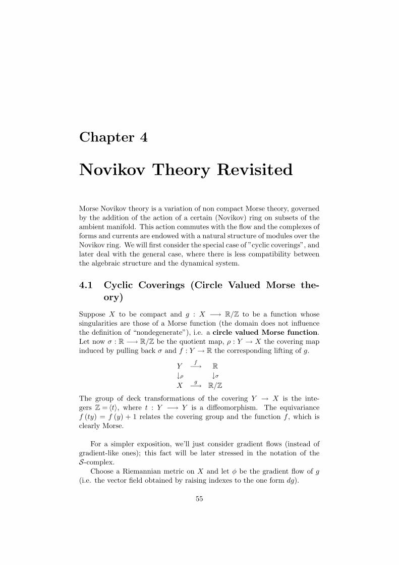
Chapter 4
Novikov Theory Revisited
Morse Novikov theory is a variation of non compact Morse theory, governedby the addition of the action of a certain (Novikov) ring on subsets of theambient manifold. This action commutes with the flow and the complexes offorms and currents are endowed with a natural structure of modules over theNovikov ring. We will first consider the special case of ”cyclic coverings”, andlater deal with the general case, where there is less compatibility betweenthe algebraic structure and the dynamical system.
4.1 Cyclic Coverings (Circle Valued Morse the-ory)
Suppose X to be compact and g : X −→ R/Z to be a function whosesingularities are those of a Morse function (the domain does not influencethe definition of “nondegenerate”), i.e. a circle valued Morse function.Let now σ : R −→ R/Z be the quotient map, ρ : Y → X the covering mapinduced by pulling back σ and f : Y → R the corresponding lifting of g.
Yf−→ R
↓ρ ↓σ
Xg−→ R/Z
The group of deck transformations of the covering Y → X is the inte-gers Z = 〈t〉, where t : Y −→ Y is a diffeomorphism. The equivariancef (ty) = f (y) + 1 relates the covering group and the function f , which isclearly Morse.
For a simpler exposition, we’ll just consider gradient flows (instead ofgradient-like ones); this fact will be later stressed in the notation of theS-complex.
Choose a Riemannian metric on X and let φ be the gradient flow of g(i.e. the vector field obtained by raising indexes to the one form dg).
55
56 Chapter 4
By pulling back via ρ, the flow φ can be lifted to a flow ψ on Y , which isthe gradient of the Morse function f (for the pullback metric). We assumeψ to be Smale (this is a generic condition).
The function f is clearly proper (hence the flow ψ is automaticallyWeakly Proper). The critical points upstairs are just the preimages of thecritical points downstairs. The main difference between the two dynamicalsystems is that upstairs there are no closed orbits (nor closed broken flowlines) whereas downstairs there might be some. Actually any flow line thathas no finite limit point downstairs lifts to a closed curve (necessarily tend-ing to ∞ in Y ).
Consider the group rings of the covering
R[t, t−1
]and Z
[t, t−1
]
i.e. the the rings of Laurent polynomials in t.
Definition 4.1.1 The (Laurent) Novikov rings
ΛR = R [[t]][t−1]
and ΛZ = Z [[t]][t−1]
are the rings of formal Laurent series with finite principal parts. In partic-ular ΛR is actually a field. Moreover ΛR is a R
[t, t−1
]-module and ΛZ is a
Z[t, t−1
]-module.
By the geometric series trick it readily follows:
Algebraic Fact 1 ΛR is a field.
Compact/forward sets can be defined algebraically, as a simple conse-quence of the interaction of the deck map t and of f :
Lemma 4.1.2 A closed set A ⊂ Y is a compact/forward set if and onlyif there exists a compact set K ⊂ Y and an integer N ∈ Z such thatA ⊂
⋃n≥N t
n (K).
Let’s now reconsider the complexes of forms and currents E∗c↑(Y ) , D′∗c↑(Y ),
C∗c↑ (Y ) , and S∗c↑ (f) defined in the previous chapter. We remark that in thissetting, the words “forward” and “compact/forward” have the same meaning(the Morse function being proper), nevertheless we mantain the terminology“compact/forward” to be consistent with the following section, dealing witha more general case.
Since the covering map t commutes with the flow ψ, the previous lemmaimplies that the action of t by pushforward is a self map of all the previous
Novikov Theory 57
complexes. This induces actions of the group rings and Novikov rings. Theoperators
T : E∗c↑ (Y ) −→ D′∗c↑ (Y )
P : E∗c↑ (Y ) −→ RS∗c↑ (f) ⊂ D′∗
c↑ (Y )
commute with the action of t by pushforward, and hence they are ΛR-linearmaps.
Theorem 4.1.3 The map of ΛR-complexes
P : E∗c↑ (Y ) −→ RS∗c↑ (f)
induces an isomorphism of finite dimensional ΛR-vector spaces
H ic↑ (Y,R) ≈ H i
(RS
∗c↑ (f)
)
Moreover, dimΛR RSkc↑ = #(critical points of index k for g) is finite.
Proof. The first statement is a direct consequence of theorem 3.2.3 and ofFact 1. In addition, any choice of a lifting p ∈ Cr (g) 7−→ p ∈ Cr(f) forthe set of critical points downstairs provides a (finite) ΛR basis for RS
∗c↑ (f),
consisting of the stable manifolds Sp ∈ RS∗c↑ at those (lifted) points ¤
The inequalities of Morse type between the dimensions (over ΛR) of
RS∗c↑ (f) and of H i
c↑ (Y,R) are an algebraic consequence of this theorem.
As for the theory with integer coefficients, a key result is:
Algebraic Fact 2 ΛZ is a principal ideal domain.
Now, observe that the inclusion map ZS∗c↑ (f) → C∗c↑ (Y ) commutes with
the action (as pushforward) of t and the complexes involved are complexesof Z
[t, t−1
]-modules as well as of ΛZ-modules. Theorem 3.2.4 then implies:
Theorem 4.1.4 The inclusion map of ΛZ-complexes
ZS∗c↑ (f) → C∗↑ (Y )
induces an isomorphism of ΛZ-modules
H i(
ZS∗c↑ (f)
)≈ H i
c↑ (Y,Z)
Moreover, ZSkc↑ is finitely generated, with one generator in ZS
kc↑ for every
critical point of g of index k (downstairs).
58 Chapter 4
Because of Fact 2, the Novikov inequalities over the integers are againan algebraic consequence of this theorem, exactly as in Morse theory.
Next we compare H∗cpt (Y,Z) and H∗
c↑ (Y,Z), in analogy with the result
in [25]. The sheaf cohomology groups Hpcpt (Y,Z) are standard topological
invariants of Y (isomorphic to Hn−p (Y,Z), i.e. homology). Altough theconstructions of T, P and the S-complex depend on f , the cohomologywith c/f supports H∗
c↑ (Y,Z) only depends on the covering translation t.Consequently, to compute the c/f supported cohomology we may replacef by a new f which is the lift to Y of a (single valued!) Morse functiong : X → R.
The isomorphism of Λ-modulesHp(
ZS∗c↑ (f)
)≈ Hp
c↑ (Y,Z) remains valid
for the new f .
But with the new f , each stable manifold Sp is relatively compact inY , therefore [Sp] has compact support and its boundary consists of a finitesum of other stable manifolds. In particular the space ZS
∗cpt (f) (made up
of finite sums of stable manifolds) is closed under taking boundary, i.e. itis a complex. Moreover, the operator P maps E∗cpt (Y ) to RS
∗cpt (f) and the
operator T is a chain homotopy between P and the identity I : E∗cpt (Y ) −→D′cpt
∗ (Y ).
Consequently, there are isomorphisms of real vector spaces and abeliangroups:
Hpcpt (Y,R) ≈ Hp
(E∗cpt (Y )
)≈ Hp
(RS
∗cpt (f)
)
Hpcpt (Y,Z) ≈ Hp
(C∗cpt (Y )
)≈ Hp
(ZS
∗cpt (f)
)
The (covering) group ring Z [π] = Z[t, t−1
]of Laurent polynomials acts
on ZS∗cpt (f) and C∗cpt (Y ). Therefore ZS
∗cpt (f) ⊗
Z[π]ΛZ and C∗cpt (f) ⊗
Z[π]ΛZ are
complexes of ΛZ modules and there are isomorphisms of ΛZ modules:
ZS∗cpt (f) ⊗
Z[π]ΛZ = ZS
∗c↑ (f) and C∗cpt (f) ⊗
Z[π]ΛZ = C∗c↑ (f)
We now need:
Algebraic Fact 3 ΛZ is flat over Z [π] = Z[t, t−1
].
By taking homology of the complexes, this implies:
Theorem 4.1.5 As finitely generated ΛZ-modules:
H∗c↑ (Y,Z) ≈ H∗
cpt (Y,ΛZ)
where, by definition, H∗cpt (Y,ΛZ) = H∗
cpt (Y,Z) ⊗Z[π]
ΛZ.
Novikov Theory 59
4.2 General Case
Let’s now look at the general case of Novikov theory. We start with a closedone form ω with nondegenerate singularities on the compact manifold X.We’ll call such forms “Novikov” forms. We recall that the irrationalitydegree of ω is the minimal number k − 1 such that all the periods of ω arerationally dependent by the periods χ1, . . . , χk. It corresponds to the small-est number of generators of ω by forms in H1(X,Z).
Let k − 1 be the irrationality index of ω and χ = (χ1, .., χk) denoteits generating periods. Let ρ : Y → X be a minimal covering such thatω pulls back to an exact form, say df , with f : Y −→ R. The group πof deck translations of (Y, ρ) is a free abelian group with k generators, sayt1, ..., tk (i.e. π ≈ Z
k) and the group rings (over R and Z) are the Laurentpolynomials rings:
R [π] = R[t1, .., tk, t
−11 , .., t−1
k
]and Z [π] = Z
[t1, .., tk, t
−11 , .., t−1
k
]
The equivariance relations f (ti (y)) = f (y) + χi hold for any i = 1, .., k.
If k = 1 the covering is cyclic and the one form ω can be seen as thedifferential of a circular valued function, which was the case in the previoussection.
Using the covering map ρ as it has been done for cyclic coverings, theform ω lifts to a Morse function f on Y . Note that f is not proper.
We choose a metric Y which is the lift of a metric on X and for whichthe gradient flow ψ of f is Smale. The gradient flow of ω on X is denotedby φ.
The critical points of f on Y are just the preimages of the critical pointsof ω on X. Of course ψ has no closed orbits (nor broken closed orbits).
Lemma 4.2.1 The lifted flow ψ is weakly proper.
Proof. Suppose γ : [0,+∞[→ Y is a forward flow-half line of ψ which isnot relatively compact in Y (i.e. γ does not converge to a critical point); wejust need to show that f is unbounded on γ. Consider the projected curveγ = ρ (γ), which is a forward flow-half line for φ. Since ρ∗ (ω) = df , and
lims→+∞
[f (γ (s))− f (γ (0))] = lims→+∞
∫ s
0
d
dtf (γ (t)) dt =
∫
γ
df =
∫
γ
ω
we are left to prove that∫γω = +∞. Observe that γ cannot converge to a
critical point for φ in X, otherwise γ would also converge to a critical pointfor ψ in Y . Moreover, for any open set D ⊂ X containing all the criticalpoints, there exists a constant c > 0, determined by ‖ω‖ on X\D, suchthat for any piece of an integral curve α contained in X\D, the estimate
60 Chapter 4
∫αω =
∫|α|2 dt > c
∫|α| dt holds. Since γ doesn’t converge to a critical
point, we can choose D so that γ has unbounded lenght in X\D ¤
Remark The previous lemma (and proof) holds for any covering where ωpullbacks to an exact form, in particular the lifted flow is weakly proper forthe universal covering.
Now we modify the classic Novikov Theory (for k > 1) by introducing anew ring. Let χ also denote the linear functional on R
k defined by χ (v) =χ·v, where χ is the vector of periods.
Definition 4.2.2 A subset F ⊂ Zk is said:
1) slab compact if F intersect each slab χ−1 ([a, b]) is compact (i.e.finite),
2) forward if F ⊂ χ−1 ([a,+∞)) for some a ∈ R,3) compact/forward or c/f if F is both slab compact and forward.
First, consider formal Laurent series α =∑ant
n , where t = (t1, .., tk)and n = (n1, .., nk). The support of α, denoted by |α|, consists of all n∈Z
k
such that an 6= 0.
Definition 4.2.3 The forward (Laurent) ring Λ consists of all formalLaurent series α =
∑ant
n with compact/forward support and with integercoefficients an ∈ Z. The alternative notations Λ = Λcf = Λ (Z) will also beused.
Note 1 The support of α is c/f if and only if |α| ∩ χ−1 ((−∞, a]) is finitefor all a ∈ R.
Note 2 Consequently, given α, β ∈ Λ, the Cauchy product γ = αβ is definedby the finite sums cn =
∑p+q=n
apbq, and γ has c/f support.
Notations. The degree of a monomial term tn is defined to be χ (n). Theset of degrees of all the non zero monomial terms in the expansion of α ∈ Λis the image χ (|α|) of the support |α| under the map χ : Z
k → R. This set
DEGS (α)def= χ (|α|) is a discrete (possibly finite) subset of R , bounded
below. Consequently, each α ∈ Λ has a unique expansion α =N≤∞∑j=0
ajtAj
with each aj non zero and deg tAj < deg tAj+1 . The degree of α is definedto be the degree of the leading term a0t
A0 .Define l : Λ → Z by taking the leading coefficient, namely l (α) = a0 (andl(0) = 0). Note that l is not a ring homomorphism, though it is a homo-morphism for the multiplicative group of Λ.
Novikov Theory 61
Lemma 4.2.4 The map l sends ideals to ideals and an element α ∈ Λ is aunit if and only if l (α) is a unit.
Proof. Let I be an ideal in Λ, and m = l(µ), n = l(ν) for some µ, ν ∈ Λthat we can suppose to be of degree zero. If m+n 6= 0 then m+n = l(µ+ν).Moreover, −m = l(−µ) and therefore l(I) is a subgroup of I. Since l is ahomomorphism for the multiplicative group of Λ, it follows that l(I) is anideal in Λ. As for the second statement, the nontrivial part is the “only if”.We can assume α = 1− β with deg (β) > 0. Since deg
(βk)
= k deg (β), thegeometric series in β provides the inverse for α in Λ (Z) ¤
As a consequence we obtain the analogous of the Algebraic Fact 1:
Corollary 4.2.5 The ring Λ (R) obtained by considering coefficients in R
is a field.
The proof of the second algebraic fact is more involved:
Lemma 4.2.6 The forward ring Λ (Z) is a principal ideal domain.
Proof. Suppose I is an ideal of Λ. Since Z is a p.i.d., l (I) = Za for some
integer a ∈ Z. Choose an element α = a+∞∑j=0
ajtAj in the ideal I with degree
zero and leading coefficient l (α) = a. Given γ ∈ I, we will inductively define
β =∞∑j=0
βj ∈ Λ (Z) so that γ = βα, proving that I = Λα.
Define γ0 = γ and, given γk ∈ I, define the monomial βk = bktBk as the
leading term of γk divided by a. Since l (I) = Za, the coefficient bk ∈ Z.Now define
γk+1 = γk − βkα = γ − (β0 + β1 + ..+ βk)α
as the error in the factorization. Thus deg βk = deg γk < deg γk+1. Putzk = deg βk: if no γk vanishes, it remains to show that lim
n→∞zn = +∞. Note
that zk = minDEGS (γk), the set of degrees of terms in γk. Let
y1, y2, ... =deg tA1 , deg tA2 , ...
= DEGS (α) \ 0
x0, x1, ... =deg tC0 , deg tC1 , ...
= DEGS (γ) = DEGS (γ0)
Now
γ1 = γ0 − β0α = C1tC1 + C2t
C2 + ...− b0a1tC0+A1 − b0a2t
C0+A2 − ...
and z0 = x0 = deg tC0 . Therefore,
DEGS (γ1) ⊂ (DEGS (γ0) ∼ z0) ∪ z0 + y1, z0 + y2, ...
62 Chapter 4
Similarly,
DEGS (γk+1) ⊂ (DEGS (γk) ∼ zk) ∪ zk + y1, zk + y2, ...
Consequently, the union of all the sets DEGS (γk) is contained in the setD of real numbers of the form xj + yi1 + ...+ yik . Since both the set of xj ’sand the set of yi’s are discrete and bounded below, the set D is also discreteand bounded below. Therefore lim
k→∞zk =∞ ¤
Exactly as in the cyclic covering case, compact/forward sets based onf can be defined algebraically in terms of the covering group Z
k.
Lemma 4.2.7 A closed set A ⊂ Y is a compact/forward set if and only ifthere exists a compact set K ⊂ Y and a c/f set F in the lattice Z
k suchthat A is contained in the union of the sets tn (K) over n ∈ F .
Theorem 4.2.8 Each of the theorems 4.1.3, 4.1.4, 4.1.5 stated in the lastsection holds for k > 1 if one substitutes the ring Λcf for Λ.
The statements and their proofs are identical, (the third algebraic factwill be proved in the next section as corollary 4.3.4), and they will not berepeated here. We just point out an important remark.
Remark (Topological Stability) Any two Novikov forms in the same co-homology class in H1 (X,R) define the same c/f sets on Y . In fact they differby the differential of a bounded function (since X is compact). Thereforetheir liftings to Y differ by a bounded function. The stability remark in thesection on Morse theory applies.
4.3 Comparison with Novikov Theory
Finally, we compare the previous results with Novikov theory (k > 1). Inorder to be concise, we will restrict to integer coefficients. It is convenientto define the Novikov ring in terms of supports.
Definition 4.3.1 A subset F ⊂ Zk is a cone-forward (or Novikov for-
ward, abbreviated n/f) set in the lattice with respect to χ if there exist a ∈ R
and ε > 0 such that F ⊂ χ−1([a,+∞)) and (”stability”) this remains truefor all χ∗ with |χ− χ∗| < ε. The Novikov ring Λnf consists of all formalLaurent series α =
∑n∈F
antn with integer coefficients whose support F = |α|
is a cone-forward set in the lattice Zk.
Note that any cone-forward set is compact/forward, so that the Novikovring Λnf is a subring of the ring Λcf . Again, the geometric power seriesargument shows that the Novikov ring Λnf (R) over R is a field.
Novikov Theory 63
Pajithnov in [26] attributes to J. Sikorav the following result; we provideda new proof for completeness.
Proposition 4.3.2 The Novikov ring Λnf is a p.i.d.
Proof. Given an ideal I ⊂ Λnf (Z), let I be the ideal in Λcf (Z) generatedby I. Pick α ∈ I, such that the ideal l (I) ⊂ Z is generated by l (α). ThenI = Λcf (Z)α. In particular, if γ ∈ I then β = γα−1 ∈ Λcf (Z), but γα−1
also belongs to Λnf (R). Finally note Λnf (Z) = Λnf (R) ∩ Λcf (Z) ¤
Proposition 4.3.3 The Novikov ring Λnf is a flat algebra over the LaurentPolynomials ring L = Z
[t1, . . . , tn, t
−11 , . . . , t−1
n
]
Proof. Let Λ+nf be the subring of the Novikov ring Λnf made up of the
elements of positive degree, and L+ the subring of L made up of polynomialsof positive degree (according to our definition of degree), so that Λ+
nf is an
algebra over L+. We now observe that Λnf can be presented as Λnf =L ⊗L+ Λ+
nf . Since ”extending the scalars” preserves flatness (cf. [B], I.2.7,
Cor. 2), we are left to prove that Λ+nf is flat over L+.
Let’s restrict to two variables, but the idea can be simply generalized tothe general case. For any α ∈ [0, π], let Λ+
α be the subring of Λ+nf made up
of series whose support in Z2 is contained in a cone of angle α centred in the
origin and symmetric with respect to the vector χ. In particular Λ+0 = Z
(since the origin is the only point of the line with direction χ and integercoordinates) and Λ+
π = Λ+nf . Let finally L+
α = L ∩ Λ+α and observe that
Λ+nf = lim−→Λ+
α , and L+ = lim−→L+αwhere the direct limit is taken for α π.
We will next prove that any Λ+α is a completion of L+
α . Since the set ofpoints with integer coordinates is discrete in the angular regions describedabove, the degree of elements in L+
α (and in Λ+α ) is a discrete (hence well
ordered) set in [0,+∞), say a0 = 0, a1, . . . , ak, . . .. Also, the sets
Iαk = λ ∈ L+α | deg (λ) ≥ ak
are ideals for L+α and the quotients
L+α /I
αk ≈ λ ∈ L
+α | deg (λ) < ak(mod Iαk )
”are” the polynomials in L+α of degree less than ak. It is the clear that
Λ+α = lim−→L
+α /I
αk , i.e. Λ+
α is a completion of L+α . Since a completion of a ring
is always flat over that ring (cf. [Ma]), the previous proves that any Λ+α is
flat over L+α .
Recall that Λ+nf = lim−→Λ+
α , and L+ = lim−→L+α , and since ,roughly speaking,
the direct limit preserves flatness (cf. [5] I.2.7, Prop. 9), it follows that Λ+nf
64 Chapter 4
is flat over L+, completing the proof of the lemma ¤
As a consequence, we get the analogous of Algebraic Fact three for thecompact/forward ring.
Corollary 4.3.4 The compact/forward ring Λcf is a flat algebra over theLaurent Polynomials ring L.
Proof Any torsion free module over a p.i.d. is flat (cf. [20]), and the com-pact/forward ring Λcf is torsion free over the Novikov ring Λnf , so Λcf isflat over Λnf . We just proved Λnf is flat over the Laurent polynomials Land since flatness has the transitive property we are done ¤
Definition 4.3.5 A closed subset A ⊂ Y is a Novikov-forward set (ab-breviated n/f-set) if there exists a compact set K ⊂ Y and a n/f set F inthe lattice Z
k such that A ⊂⋃n∈F
tn (K)
The Novikov-forward sets are compact/forward with respect to f , sincef (tn (y)) = χ · n + f (y). The converse is not always true if k > 1 becausethe lattice contains compact/forward sets which are not Novikov/forward.
Clearly, each covering translation ti acts on the various complexes offorms and current with support in Novikov/forward-sets and the differentactions commute (since the ti’s do). This allows one to define actions of thegroup ring and Novikov ring ”by linearity” on those complexes; the supportsare in fact preserved by the action of the Novikov ring Λ. One can also definean S-complex ZS
∗nf with supports in n/f -sets and all the previous arguments
carry over substituting n/f -sets for compact/forward sets with respect to f .
Theorem 4.3.6 Each of the Theorems 4.1.3, 4.1.5, 4.1.5 stated for cycliccovers holds for the (k > 1) Novikov case if one substitutes n/f-supports forcompact/forward supports.
Again, the statements and their proofs are identical and will not berepeated here. These three theorems in the n/f case and the c/f are directlyrelated as follows. Since Λcf (R) is a field, Λcf (Z) is a torsion free moduleover the ring Λ = Λnf (Z). Since the ring Λ = Λnf (Z) is a p.i.d., this impliesthat Λcf (Z) is a flat Λ-module. Therefore:
ZS∗c↑ ≈ ZS
∗nf ⊗Λ Λcf (Z)
H∗c↑ (Y,Z) ≈ H∗
(ZS
∗c↑
)≈ H∗
(ZS
∗nf
)⊗Λ Λcf ≈ H
∗nf (Y,Z)⊗Λnf
Λcf
In particular the Novikov numbers and inequalities are the same over Λnf
or Λcf .

Novikov Theory 65
The larger ring Λcf (Z) is geometrically more natural in the contextof non-compact Morse Theory, while the smaller ring Λnf (Z) has otheradvantages. Of course they coincide in the cyclic (k = 1) case.
4.4 Lambda Duality
Let ΛZ denote either the compact/forward or the Novikov ring, and let ΛR
denote the corresponding field. First, consider the field Λ = ΛR, subscriptsare understood. Each critical point x0 ∈ X, of index h, determines a Λ-linein Shc↑ denoted Shx0
which equals Λ [Sy0 ] where y0 is any fixed critical point
above x0. Each S ∈ Shx0uniquely determines λ ∈ Λ for which S = λ · [Sy0 ].
Similarly, each critical point x0 ∈ X, of index h determines a Λ-line in Un−hc↓ ,
denoted Un−hx0, which consists of all sums U =
∑n∈|µ|
bnUt−ny0 = µUy0 , where
µ =∑n∈|µ|
bntn ∈ Λ. As before, U ∈ Un−hx0
uniquely determines µ ∈ Λ with
U = µUy0 .
Note. The same Λ acts on S and U ; necessarily, then, the variable t actsby pullback on U and in particular the line Un−hx0
⊂ Un−hn↓ ⊂ Un−hc↓ .
Definition 4.4.1 Given U ∈ Un−hx0and S ∈ Shx0
define the Λ -pairing of Uand S by
(U, S)Λ = λµ
where U = µUy0 and S = λSy0 determine λ and µ.
Lemma 4.4.2 The pairing ( , )Λis Λ-bilinear and independent of the choiceof the critical point y0 ∈ Y above x0 ∈ Cr (ω) ⊂ X.
Proof. Suppose y′0 is another choice of critical point above x0. ThenSy′
0= Stny0 = tnSy0 while Uy′
0= Utny0 = t−nUy0for the same n ∈ Z so
that λ = λ′tn and µ = µ′t−n and λµ = λ′µ′ ¤
Note that Sh =∑
x∈Cr(ω,Ind h)
Shx and Un−h =∑
x∈Cr(ω,Ind h)
Un−hx . Given
S ∈ Sh and U ∈ Un−h the Λ-bilinear pairing obviously extends to (S,U)Λ.
Remark If (S • U) denotes the current intersection of S with U paired with1 (i.e. the number of points in the intersection), then (S • U) ∈ Z is theleading coefficient of (S,U)Λ ∈ Λ.
Theorem 4.4.3 The Λ-vector spaces Shc↑ and Un−hc↓ are finite dimensionaldual vector spaces under the pairing ( , )Λ. Consequently, the Λ-vector
spaces Hh(S∗c↑
)and Hn−h
(U∗c↑
)are Λ-dual finite dimensional vector spaces.
66 Chapter 4
The proof is immediate.The integer case produces two finitely generated complexes of ZΛ-bilinear
pairing; and with bases Si, Ui so that (Si, Uj) = δij . It follows algebraicallythat Λ-Poincare duality holds over Z.
Chapter 5
Functions and 1-forms withBott Singularities
5.1 The Boundary Value Technique
We now present a generalization of the theory discussed in section 1.3, adapt-ing it to the case of Bott singularities. The arguments are often very similar,so the proof are sometimes omitted or sketched. Again, no part of this sec-tion is completely original, and we refer to the sources quoted before asreferences.
Definition 5.1.1 Let V be a vector field on a manifold X of dimension nand C ⊂ X a regular (hence closed) submanifold of dimension c. SupposeV |C = 0. The singular points on C are called of “Bott” type or “nonde-generate in the normal direction” if for any point p ∈ C there existslocal coordinates u, v near p such that C = u = 0 and the local systemdetermined by V has the form
u = Au+ a(u, v)v = b(u, v)
where A is a square matrix of order n− c with no purely imaginary in-variant and a and b are vector valued functions which vanish on C togetherwith their differentials.The number λC = (λp) of negative characteristic exponents of the matrix Ais called the index of C (or of any p ∈ C). We also put, following [18],λ∗C = n− c− λC .
A function f : X → R or a one form ϕ ∈ E1(X) is called “Morse-Bott” if for some (and hence all) Riemannian metric, the singularities of thecorresponding gradient vector field are of Bott type, distributed on compactcritical manifolds.
67
68 Chapter 5
Consider the following system on Rs × R
u × Rc:
x = L−x+ f(t, x, y, z, θ)
y = L+y + g(t, x, y, z, θ)
z = h(t, x, y, z, θ)
(5.1)
where the matrices L− and L+ are in Jordan form, the real parts of theeigenvalues of L− are strictly negative, say −λs ≤ · · · ≤ −λ1 < 0, and thoseof L+ strictly positive, say 0 < µ1 ≤ · · · ≤ µu.
In the sequel the symbol |x, y, z| will always mean the max among|x|, |y|, |z|. Now set:
F = (f, g, h) : R× Rs × R
u × Rc ×W → R
s × Ru × R
c
We assume that F vanishes on the critical manifold C = 0× Rc and the
spatial derivatives of the non linear terms are uniformly bounded, i.e. thereexists δk such that:
F (t, 0, 0, z, θ) = 0
δkεdef= sup
|x,y|≤ε
∑
|m|=k
∣∣∣ ∂kF∂(x,y,z)m
∣∣∣ ≤ δk < +∞ (5.2)
Note that the bounds δkε are taken over tubular neighborhoods of thecritical manifold.
Lemma 5.1.2 In the previous hypotheses, the following inequalities hold:
|F (t, x, y, z, θ)| ≤ δ1|x,y||x, y| (5.3)
|∂kF
∂zk(t, x, y, z, θ)| ≤ δk+1
|x,y||x, y| (5.4)
Proof. By F (t, 0, 0, z, θ) = 0 it follows ∂kF∂zk (t, 0, 0, z, θ) = 0; then apply the
mean value theorem ¤
Definition 5.1.3 We say that the Boundary Value problem (abridgedB.V. problem) with data (x0, y1, z1, τ) ∈ R
n × [0,+∞) is solvable for thesystem 5.1 if there exists a solution (x∗(t), y∗(t), z∗(t)) defined on [0, τ ] andsatisfying:
(x∗(0), y∗(τ), z∗(τ)) = (x0, y1, z1)
Theorem 5.1.4 Suppose the estimate 2δ1 < α hold. Then the BoundaryValue problem for the system 5.1 is solvable for any data (x0, y1, z1, τ). Thesolution is unique, it depends smoothly on (t, x0, y1, z1, τ, θ) and satisfies:
|x∗ (t) , y∗ (t) | ≤ 2|x0, y1| for any t ∈ [0, τ ] (5.5)
Bott Singularities 69
Notations In the same way as for an Initial Value problem, a BV problemis denoted by:
x = L−x+ f (t, x, y, z, θ)y = L+y + g (t, x, y, z, θ)z = h(t, x, y, z, θ)
x∗(0) = x0, y∗(τ) = y1, z
∗(τ) = z1
(5.6)
The solutions to Initial and Boundary Value problems will be denoted asin section 1.3; we just recall the “end point map” (x∗1, y
∗0, z
∗0) for the BV
solution, defined as:
x∗1 (x0, y1, z1, τ) = x∗ (τ, x0, y1, z1, τ) (5.7)
y∗0 (x0, y1, z1, τ) = y∗ (0, x0, y1, z1, τ) (5.8)
z∗0 (x0, y1, z1, τ) = z∗ (0, x0, y1, z1, τ) (5.9)
It is useful to join the “unstable variables” y, z under a single coordinate
wdef= (y, z). For example, the discussion after theorem 1.3.3 works word for
word by replacing y with w and therefore proving:
Corollary 5.1.5 The following matrices are invertible and
(∂w∗
∂w1|(t,x0,w1,τ)
)−1
=∂w
∂w0|(t,x0,w
∗0(x0,w1,τ))
(∂w∗
0
∂w1|(x0,w1,τ)
)−1
=∂w
∂w0|(τ,x0,w
∗0(x0,w1,τ))
Proof of the theorem. This time the system of integral equations is:
x(t) = etL−x0 +
∫ t0 e
(t−s)L−f(s, x(s), y(s), z (s) , θ)ds
y(t) = e−(τ−t)L+
y1 −∫ τte(t−s)L
+
g(s, x(s), y(s), z (s) , θ)dsz (t) = z1 −
∫ τth(s, x(s), y(s), z (s) , θ)ds
(5.10)
Fact 5.1 Any continuous curve, solution of the equations (5.10) is necessar-ily smooth in t and is a solution to the BV problem with data (x0, y1, z1, τ).The viceversa is also true.
70 Chapter 5
The right hand side of the equations (5.10) defines an operator on thespace of continuous curves: its fixed points are our target. In order to makeit a contraction, we consider a weighted norm for the curves.
Choose any γ such that = δ1 < γ < α/2 and denote by γVτ the Banachspace C0 ([0, τ ] ,Rn) of continuous curves endowed with the γ-weighted norm
‖X = (x (t) , y (t) , z (t))‖γ = sup[0,τ ]
(|x (s) , y (s) , z (s) |eγs)
Define T : γVτ × Rn ×W → γVτ by acting on (X(t), x0, y1, z1, θ) as:
T x (X) (t) = etL−x0 +
∫ t0 e
(t−s)L−f(s, x(s), y(s), z(s), θ)ds
T y (X) (t) = e−(τ−t)L+
y1 −∫ τte(t−s)L
+
g(s, x(s), y(s), z(s), θ)ds
T z (X) (t) = z1 −∫ τth(s, x(s), y(s), z(s), θ)ds
Claim 5.1 T is continuous (on γVτ × Rn ×W ).
As before, this can be simply checked directly.
Claim 5.2 T is C∞ in the γVτ arguments.
Proof. The differentials dkT in the V arguments are the linear operators
dkTX(X ′
1, . . . , X′k
)(t) =
∫ t0 e
(t−s)L−dkf |(s,X(s),θ) (X ′
1 (s) , . . . , X ′k (s)) ds
∫ τte(t−s)L
+
dkg|(s,X(s),θ) (X ′1 (s) , . . . , X ′
k (s)) ds
∫ τte(t−s)L
+
dkh|(s,X(s),θ) (X ′1 (s) , . . . , X ′
k (s)) ds
where X,X ′i ∈ V , and dkf . . . are the differentials in the spatial direc-
tions. In fact let’s just check Taylor’s formula:
Bott Singularities 71
ψ(t) =∣∣∣(T (X+X ′)− T (X)− dTXX
′ −. . .− dT kX(X ′,. . .,X ′
))(t)∣∣∣ ≤
≤ sup
∫ t0 e
−α(t−s)|f(s,X+X ′)−f(s,X)−∑k
i=1 dif |(s,X(s),θ)(X
′,. . .,X ′) |ds
∫ τteα(t−s)|g(s,X+X ′)−g(s,X)−
∑ki=1 d
ig|(s,X(s),θ)(X′,. . ., X ′) |ds
∫ τt|h(s,X+X ′)−h(s,X)−
∑ki=1 d
ih|(s,X(s),θ) (X ′,. . ., X ′) |ds
≤ sup
∫ t0 e
−α(t−s)δk+1‖X‖+‖X′‖
|X′(s)|k+1
k+1! ds
∫ τteα(t−s)δk+1
‖X‖+‖X′‖
|X′(s)|k+1
k+1! ds
∫ τtδk+1‖X‖+‖X′‖
|X′(s)|k+1
k+1! ds
≤δk+1‖X‖+‖X′‖
k + 1!‖X ′‖k+1
γ sup
∫ t0 e
−αt+(α−(k+1)γ)sds∫ τteαt−(α+(k+1)γ)sds
∫ τte−(k+1)γsds
Hence we get
ψ(t)eγt ≤δk+1‖X‖+‖X′‖
min(k + 1)γ, |(k + 1)γ − α|(k + 1!)‖X ′‖k+1
γ
which provides an estimate (uniform in τ) for the C∞ smoothness of T .
Claim 5.3 T is a contraction on γVτ . In fact ‖dT‖γ <δ1
γ(which is < 1
by hypothesis).
Proof. We can easily check dT to be a contraction (here δ means δ1):
∥∥dTXX ′ (t)∥∥γ
= sup[0,τ ]
eγt
∣∣∣∫ t0 e
(t−s)L−df |(s,X(s))X
′ (s) ds∣∣∣∣∣∣
∫ τte(t−s)L
+
dg|(s,X(s))X′ (s) ds
∣∣∣∣∣∫ τtdh|(s,X(s))X
′ (s) ds∣∣
≤ sup[0,τ ]
eγt
∫ t0 e
−α(t−s)δ‖X‖|X′ (s) |ds∫ τ
te(t−s)L
+
δ‖X‖|X′ (s) |ds∫ τ
tδ‖X‖|X
′ (s) |ds
≤ δ‖X‖
∥∥X ′∥∥γsup[0,τ ]
eγt
∫ t0 e
−α(t−s)e−γsds∫ τteα(t−s)e−γsds∫ τ
te−γsds
≤δ‖X‖
γ
∥∥X ′∥∥γ
72 Chapter 5
And therefore ‖dTX‖γ ≤δ
γ< 1 ¤
Remark The estimate 2δ1 < α assumed as hypothesis differs from the sim-ilar estimate δ1 < α assumed in the case of isolated singularities. In the lastinequality proven, in fact, we needed at the same time δ < γ and δ < α− γ,and hence δ1 < α was not sufficient.
Because of the previous claim, the contraction lemma provides the ex-istence of unique fixed points for the operator T for any choice of data(x0, y1, z1, τ), solving the existence and uniqueness issue for the BV prob-lem.
Claim 5.4 Fix (x0, y1, z1, θ) and a curve X(t) = (x(t), y(t), z(t)). If theinequality |x(t), y(t)| ≤ 2|x0, y1| holds, then |T x(X)(t), T y(X)(t)| ≤ 2|x0, y1|for the first components of T (X) too.
Proof. Exactly as Claim 1.4; the γ norm is not involved here.
Claim 5.5 The operator T : Vτ × Rn ×W → Vτ is C∞ regular.
Proof. T is affine in the spatial data (x0, y1, z1) and the parameters θcan be considered as new variables adding them to “z” via the constantequation θ = 0. Since T is continuous, the theorem about differentiabilityafter regularity of partial derivatives proves the claim.
By now, the proof of smooth dependence of solutions on the variables(x0.y1, z1, θ) goes on exactly as in the case of nondegenerate singularities,relying upon the implicit function theorem in Banach spaces. The same ar-guments as before (replacing the variables y, z by w and using corollary 5.1.5)works word for word in the present case, proving the smooth dependence ofthe solution to a BV problem on τ and completing the proof of the existenceand uniqueness theorem ¤
The derivatives of the solutions to a BV problem certainly satisfy thecorresponding variational differential systems. Moreover, as in the case ofisolated singularities, the variational systems are in the same form as system5.1. The proof given for corollary 1.3.5 then shows:
Corollary 5.1.6 Under the hypothesis of the existence and uniqueness the-orem 5.1.4, the derivatives to the BV problem 5.6 with respect to the spatialBV data x0, y1, z1 and parameters θ can be found as solutions to the BVproblem whose equations are the variational equations and the new BV dataare given by formal differentiation of the old ones. In particular the BV dataare zero for the derivatives in θ or anyway for derivatives of second orderand higher.
Bott Singularities 73
The derivatives in t for the solutions are described by the differentialequations themselves (of the original system or of the variational ones),whereas for the τ variable, the discussion in section 1.3 goes through wordfor word if one here substitutes w = (y, z) to the variables y there.
Corollary 5.1.7 The derivatives of the BV solutions in τ satisfy:
∂x∗
∂τ|(t,x0,w1,τ) = −
∂x∗
∂w1|(t,x0,w1,τ)
∂w∗
∂t|(τ,x0,w1,τ) (5.11)
∂w∗
∂τ|(t,x0,w1,τ) = −
∂w∗
∂w1|(t,x0,w1,τ)
∂w∗
∂t|(τ,x0,w1,τ)
Theorem 5.1.8 The first derivatives of the endpoint map satisfy:
∂x∗1∂x0, w1, θ
|(x0,w1,τ) =∂x∗
∂x0, w1, θ|(τ,x0,w1,τ) (5.12)
∂w∗0
∂x0, w1, θ|(x0,w1,τ) =
∂w∗
∂x0, w1, θ|(0,x0,w1,τ) (5.13)
∂x∗1∂τ|(x0,w1,τ) =
∂x∗
∂t|(τ,x0,w1,τ) −
∂x∗
∂w1|(τ,x0,w1,τ)
∂w∗
∂t|(τ,x0,w1,τ) (5.14)
∂w∗0
∂τ|(x0,w1,τ) =
∂w∗
∂τ|(0,x0,w1,τ) (5.15)
The kth derivatives of the endpoint map are linear combinations of deriva-
tives∂hx∗
∂ht, x0, w1, θ|τ,x0,w1,τ and
∂hw∗
∂ht, x0, w1, θ|0,x0,w1,τ with 0 ≤ h ≤ k, the
coefficients being products of other derivatives of x∗ and w∗.
Hypothesis From now on, the differential system is supposed to be localand autonomous, i.e. of the form:
x = L−x+ f (x, y, z)y = L+y + g (x, y, z)z = h(x, y, z)
(5.16)
The non linear terms F = (f, g, h) are just defined locally near the ori-gin, and satisfy F (0, 0, z) = 0 and dF |(0,0,z) = 0.
In the new hypothesis, there exists a small enough neighborhood of theorigin U ⊂ R
s×Ru×R
c where the estimate 2δ1 ≤ α on the first derivativesholds. Modifying the system 5.16 away from U by a smooth cut off, theexistence and uniqueness theorem 5.1.4 applies, and its thesis then holds onU for system 5.16 as well, thanks to the bound given by relation 5.5. Wecan now prove:
74 Chapter 5
Theorem 5.1.9 (Stable Bundle) For any point z in Rc ∩U there passes
a unique invariant manifold Sz of dimension s called “stable manifold forz” which is the union of trajectories in U tending to z. The union S = ∪Szis a C∞ bundle over the critical manifold R
c called the “stable bundle” andit is made up of all the trajectories which stay bounded in a neighborhood of0 for all times.
Proof. Using the cut off trick,it’s sufficient to assume the nonlinear termsto be globally defined and the bound on their first derivatives to hold on allof R
n.
Fix now a z1 ∈ C and translate the system X = F (X) so that z1 = 0.The new system is just X = F (X − (0, 0, z1)), which we can consider asa system depending on the “nonspatial” parameter z1. Consider now theBanach space V of continuous curves defined on the half line and boundedin the γ-weighted norm, for some 2δ < γ < α.
The choice z1 = 0 allows the integral operator T associated to 5.16 tooperate on V for τ =∞. In fact T is now given by:
T x (X) (t) = etL−x0 +
∫ t0 e
(t−s)L−f(s, x(s), y(s), z(s), z1)ds
T y (X) (t) = −∫ +∞t
e(t−s)L+
g(s, x(s), y(s), z(s), z1)ds
T z (X) (t) = −∫ +∞t
h(s, x(s), y(s), z(s), z1)ds
Observe that z1 is considered as one of the old “θ” parameters. Allthe estimates in the proof of theorem 5.1.4 still work for the new T , sincethey never involved τ explicitly. Therefore, for any fixed z1 and for any x0
there is a solution x∗(t), y∗(t), z∗(t), defined on the half-line, which con-verge exponentially (faster than e−γt) to the point (0, 0, z1). One thengets a smooth “endpoint” map (x0, z1)→ (y∗0(x0, z1), z
∗0(x0, z1)). Note that
(y∗0(0, z1), z∗0(0, z1)) = (0, z1). Therefore, the graph S of the endpoint map
is a smooth manifold of dimension s + c and is the disjoint union of thesubmanifolds Sz1 , graphs of the restrictions of the endpoint map to z = z1.Of course, S is the stable bundle and its fibers Sz1 the unstable manifolds.In fact, similarly to the case of isolated singularities, one proves that Sz1is invariant by the flow and contains any solution which is bounded in theγ-norm after translation in (0, 0, z1), i.e. any solution which tend to (0, 0, z1)faster than e−γt (for any 2δ < γ < α).
The fact that all bounded small solutions actually belong to the stablebundle can be seen using the estimates we’ll later prove ¤
Remark Repeating all the discussion by considering z as a stable coordi-nate (i.e. treating z as the x coordinates instead that as the y ones) providesanalogous results. In particular there exists the “unstable bundle” of thecritical manifold C whose fibers are the “unstable manifolds” for the points
Bott Singularities 75
in C.
Using an analogous of lemma 1.3.13, it is not difficult to check thetransversalities needed to state the following:
Corollary 5.1.10 (Straighten Coordinates) After a smooth change ofcoordinates, the system 5.16 can be written as
x = L−x+ f(x, y, z)xy = L+v + g(x, y, z)yz = h(x, y, z)xy
(5.17)
where f, g, h are square matrices of smooth functions vanishing on the crit-ical manifold R
c and h(x, y, z)xy stands for a vector whose components aresums of terms each of which factors through xiyj, for some i, j. The newcoordinates are called straighten coordinates since the stable and unstablemanifolds in z0 are given by y = 0, z = z0 and x = 0, z = z0 respectively.
In straighten coordinates, useful estimates hold on the size of the solu-tion. Again, the “not leaving the neighborhood” issue (usually needed forthis kind of estimates) is simple to deal with, for solutions to BoundaryValue problems, since these are confined by construction.
Theorem 5.1.11 Suppose |x0, y1| ≤ ε. Then for any τ ∈ [0,+∞) thefollowing inequality hold, for some constant C0 independent on τ :
|x∗(t, x0, y1, τ)| ≤ |x0|e−(α−δ)t
|y∗(t, x0, y1, τ)| ≤ |y1|e(α−δ)(t−τ)
|z∗(t, x0, y1, τ)− z1| ≤ C0τe−δτ
(5.18)
|x∗1(x0, y1, τ)| ≤ |x0|e−(α−δ)τ
|y∗0(x0, y1, τ)| ≤ |y1|e−(α−δ)τ
|z∗0(x0, y1, τ)− z1| ≤ C0τe−δτ
(5.19)
Proof. The Gronwall lemma, applied exactly as in the proof of theorem1.3.16 proves the estimates on the x, y variables, since nothing formallychanges. As for z, observe that
z(t)− z1 = −
∫ τ
t
h (x(s), y(s), z(s))x(s)y(s)ds
so that the thesis follows, bounding h by δ ¤
As for the derivatives of the solutions, we observe that the variationalsystems for derivatives of order k in the x, y, z or t variables have the form:
76 Chapter 5
Xk = L−Xk + f(x∗, y∗, z∗)Xk + (· · · )Xk−1 + . . .+ (· · · )x˙Y k = L+Y k + g(x∗, y∗, z∗)Y k + (· · · )Y k−1 + . . .+ (· · · )y
Zk =∑
(· · · )(X iY h−i)
(5.20)
This means that each summand in the first equation factors trough somelower order derivatives of x (and similarly in the second), whereas in thethird equation all addenda factor through products of derivatives of x andy (of course 0 ≤ h ≤ k in the formula).
Theorem 5.1.12 Suppose ε > 0 is such that kδ < α. Let X∗(t), Y ∗(t) besome kth-order derivatives of (x∗, y∗) in the spatial variables x0, y1 and/orin the time variables t, τ . The following inequalities hold, for some constantCk > 0:
|X∗(t)| ≤ Cke−(α−kδ)t
|Y ∗(t)| ≤ Cke(α−kδ)(t−τ)
|Z∗(t)| ≤ Ckτe−(α−kδ)(τ)
Proof. The proof of the first two inequalities is exactly the same as intheorem 1.3.18 since the expressions are formally the same. It remains todeal with Z∗. Since Z∗ solves
Z(t)− Z1 = −
∫ τ
t
∑(· · · (s))(X i(s)Y h−i(s))ds
The dots are bounded by a uniform constant depending on the estimateson the derivatives f, g, h, whereas |X i(s)Y h−i(s)| ≤ Ce(α−kδ)τ where C de-pends on the constants coming from the estimates of X i and Y h−i and onthe number of terms involved. Integrating gives the thesis ¤
By theorem 5.1.8, in the same hypothesis of the previous theorem, itthen follows (again w stands for (y, z)):
Theorem 5.1.13 Let V ∗(τ) denote some derivative among∂kx∗1
∂kx0, w1,τ|(x0,w1,τ)
or among∂kw∗
0
∂x0, w1, τ|(x0,w1,τ). Then the following inequality holds, for some
constant Ck > 0, not depending on x0, w1, τ :
|V ∗(τ)| ≤ (1 + τ)Cke−(α−kδ)τ
Conclusions We finally draw out the consequences which will be used later.For the sake of clearness we repeat all the hypothesis here.
Bott Singularities 77
Consider a vector field on Rn = R
s × Ru × R
c having Rc as critical
submanifold of Bott singularities. Let φ = (φt)t∈R be the (local) flow ofsolutions near a critical point, which we assume to be the origin. Thenthere exists “straighten coordinates” x, y, z near the origin for which S =y = 0 is the stable bundle and Sz1 = y = 0, z = z1 the stable manifolds,U = x = 0 the unstable bundle and Uz1 = x = 0, z = z1 the unstablemanifolds.
Consider then the unit cylinder B = (x, y, z)| |x, y, z| < 1 and decom-pose its boundary ∂B in the pieces:
∂+B = |x| = 1, |y, z| ≤ 1, ∂−B = |x, z| ≤ 1, |y| = 1∂cB = |z| = 1, |x, y| ≤ 1,
We can suppose that ∂−B and ∂+B are transversal to the vector field (atleast for small z) and that if a point m ∈ ∂−B does not belong to thestable bundle S and is distant from ∂cB, then the trajectory starting fromm will touch ∂B again in ∂+B. This is granted by corollary 5.1.10 and theestimates in theorem 5.1.11. The construction defines a “first escape” map
ϕ : ∂+B\S → ∂−B\U
Since the vector field is not tangent to ∂±B and the flow of solutions is asmooth map, an application of the implicit function theorem proves
Theorem 5.1.14 The first escape map ϕ : ∂−B\S → ∂+B\U is a diffeo-morphism onto its image.
Now, consider the submanifold
W = (φ t
1−t(m),m, t
)|m ∈ R
n, t ∈ (0, 1) ∩ B ×B × (0, 1) ⊂ R2n+1
Theorem 5.1.15 The closure W = (W,∂W ) is a smooth, closed submani-fold in ×B ×B × R with boundary
∂W = U ×C S × 1 ∪ ∆× 0
where
U ×C S = (0,y,z,x,0,z) ∈ Rn × R
n
is the fiber product of the stable and unstable bundles, which is a smoothsubmanifold of dimension n.
Proof. Using the starred notation for the solution to the BV problem, bythe existence and uniqueness theorem one can reintrepret W as:
78 Chapter 5
W =(φ t
1−t(x0, y0, z0), x0, y0, z0, t
) ∣∣ (x0, y0, z0) ∈ Rn∩B ×B × (0, 1)
=(x∗1(x0, y1, z1, τ
1−τ
), y1, z1, x0, y
∗0
(x0, y1, z1, τ
1−τ
), z∗0 , τ
) ∣∣ |x0, y1, z1| < 1τ ∈ (0, 1)
so that the estimates in theorem 5.1.13, combined with the same invarianceargument given for theorem 1.3.21 permit to conclude ¤
5.2 Vector Fields and One Forms with Bott Sin-gularities
All over this section X will denote an oriented (not necessarily compact)n-dimensional manifold, V a complete vector field and φ the correspondingflow. The vector field is supposed to have Bott singularities distributedalong compact oriented (critical) submanifolds.
Using the notations UC (resp. SC) for the unstable bundle (resp. sta-ble bundle) of the critical manifold C and Up (resp. Sp) for the unstablemanifold (resp. stable) of the critical point p, we introduce the following:
Definition 5.2.1 The flow φ satisfies the generalized Smale conditionif all the intersections between stable bundles and unstable manifolds and be-tween stable manifolds and unstable bundles are transversal. In other words,for any critical points and critical manifolds p ∈ Cp and q ∈ Cq, the inter-sections SCp ∩ Uq and Sp ∩ UCq are transversal.
We assume the flow φ to satisfy the generalize Smale condition and thevector field V to be Weakly Proper with respect to some smooth functionf : X → R. Note that for a vector field with Bott singularities it’s enough tocheck the Weakly Proper hypothesis just on points instead than on compactsets, cf. proposition 2.1.3.
Under these hypotheses, any critical manifold is contained in a level setof f . Two critical manifolds C and C ′ cannot intersect and if there is a (pos-sibly broken) flow line connecting C and C ′ then the inequalities λC < λC′
and λ∗C′ < λ∗C hold between the corresponding indexes.
Remark Contrary to the case of Morse functions, it is not true that anyfunction f with Bott singularities always admits a metric such that the gra-dient vector field ∇f is generalized Smale, cf. [18] for an example.
We will next show how to generalize the results of chapters 2 and 3 toflows of vector fields with Bott singularities, starting with the following:

Bott Singularities 79
Definition 5.2.2 A compact stratified set Y of dimension k will be calledcompact generalized horned-stratified (or compact gh-stratified) setif:
• The stratification of Y is AB Whitney regular;
• There exists a k-dimensional compact manifold with corners M , a re-finement of the stratification of M to an AB regular stratification whichdoes not modify the interior of M , and a submersive stratified mapπ : M → Y .
The manifold M with the refined stratification is called a desingularizationfor Y and the map π a gh-projection.
A locally gh-stratified set Y ⊂ X is a stratified set which locallycoincide with a compact generalized horned stratified set.
Remark. The A-regularity requirement for Y in the previous definition isgranted by the existence of the desingularization M → Y . Observe, more-over, that the refinement of the stratification on M is not supposed to belocally finite. It is often needed, for example, to consider a two dimensionalface as stratified by one dimensional submanifolds.
The arguments in section 2.2 work in the present setting by replacing h-stratified with gh-stratified and giving to “desingularizing” the new meaningof definition 5.2.2. The only point to keep in mind is the double nature ofthe desingularization: as manifold with corners and as a stratified set. Asan example, we prove the following:
Proposition 5.2.3 Let Y ⊂ X be a gh-stratified set and Z ⊂ X a closedsubmanifold. Suppose that each stratum of Y is transversal to Z. Then thefamily of all intersections of strata makes up a gh-stratification for Z ∩ Y .
Proof. It’s enough to find a desingularization for Z ∩Y . Let π : M ⊂ N →X be a local desingularization for Y . By hypothesis, the restriction of π toany stratum of M (both as a manifold with corners and as a stratified space,after the refinement) is transversal to Z and thus M ∩ f−1(Z) is endowedwith both the structures of compact manifold with boundary and AB reg-ular stratification (by refinement of the corners). The restriction of π is agh-projection, because of lemma 2.2.5 ¤
Referring to section 2.2 for the proofs, that basically work word for wordas observed above, we just state:
Proposition 5.2.4 Let Y1, Y2 ⊂ X be gh-stratified sets and suppose that allpossible intersections of strata of Y1 and Y2 are transversal. Then the familyof these intersections is a gh-stratification for Y = Y1 ∩ Y2.

80 Chapter 5
Corollary 5.2.5 Let Y1, Y2 ⊂ X be gh-stratified sets and y ∈ Y1 ∩ Y2. Ifthe two strata containing y intersect transversally, then all the strata neary intersect transversally and hence, near y, the intersection Y1 ∩ Y2 is agh-stratified set.
Remark In the case of h-stratifications, the local desingularizations define“h-chain” currents by pushforward under some orientability assumption. Forgh-stratifications one might still define “gh-chain currents” by pushforward(assuming the desingularizations are oriented maps), but such a family wouldnot be close under the boundary operation and so we’ll not pursue this aim.Nevertheless the pushforward of a gh-projection is a quite special chaincurrent, in fact (cf. proposition 2.2.15):
Proposition 5.2.6 Let [T ] be a k-dimensional chain current in Rn locally
defined as the pushforward π∗(M) under the gh-projection π : M → T of thegh-stratified space T . If [S] is chain current of dimension l and the simplexeswhich locally define S are transversal to the strata of T , then [S] and [T ]can be “intersected” and [S]∧ [T ] = [S ∩ T ] is a chain current of dimensionh+ k − n.
Keeping the notations introduced in section 2.3, we can now state thefollowing generalization of theorem 2.3.1:
Theorem 5.2.7 Let (X,φ, f : X → R) be a Weakly Proper generalizedSmale dynamical system, c ∈ R a regular value for f and M ⊂ f−1(c) asmooth (embedded) submanifold of dimension m. Suppose M is transversalto every stable manifold and let N =
⋃t>0
φt(M). Then the closure N coin-
cides with the shadow LM and it is a gh-stratified subset of dimension m+1whose singular strata are unstable manifolds.
As in the case of isolated singularities, one also gets the following:
Corollary 5.2.8 The unstable bundle UC of a critical manifold C (resp. theunstable manifold Up of a critical point p) is a generalized horned stratifiedsubset whose singular strata are the unstable manifolds in the shadow of C(resp. p). Similarly for stable bundles and manifolds.
The proof given for the analogous theorem 2.3.1 is still valid for theprevious theorem, but its preliminary results (propositions 2.3.4 and 2.3.5)need to be modified to fit in the new frame. We thus just prove the twoadequate extensions.
Suppose p is a critical point belonging to the critical manifold C. We fixa chart Ω in “straighten coordinates” x, y, z centred in p (cf. the previous
Bott Singularities 81
section). The boundary of Ω decomposes as ∂Ω = ∂+Ω∪∂−Ω∪∂cΩ , where
∂+Ω = ‖x‖ = ε, ‖y, z‖ ≤ ε
∂−Ω = ‖x, z‖ ≤ ε, ‖y‖ = ε
∂cΩ = ‖x, y‖ ≤ ε, ‖z‖ = ε
Note that the third component of boundary is not necessarily invariantby the flow. Define the “links” of (un)stable bundles and manifolds as:
S+ = S ∩ ∂+Ω = ‖x‖ = 1, y = 0 , S+z = Sz ∩ ∂
+Ω
U− = U ∩ ∂−Ω = ‖y‖ = 1, x = 0 , U−z = Uz ∩ ∂
−Ω
We can now prove the analogous of the “second brick” in the proof oftheorem 2.3.1 :
Proposition 5.2.9 Suppose A+ ⊂ ∂+Ω is a compact manifold with cornerssuch that all strata have transversal intersection with S. Put
A = φt(x)|x ∈ A+, t > 0 ∩ Ω
Then the closure A coincides with the shadow LA+
Ω and is a compact gen-eralized horned stratified set. Its singular strata (besides the shadows of thestrata in A+) are unstable manifolds.
The closure of A− def= A ∩ ∂−Ω is gh-stratified too. Its singular strata
are links of unstable manifolds (and of the shadows of the strata in A+).
Remark The shadow of A+ does not touch ∂cΩ at all provide Ω is smallenough and A+ is well disjoint by ∂cΩ, thanks to the estimates in theorem5.1.11.
Proof. We restrict to the case when A+ ⊂ ∂+Ω is a smooth compactsubmanifold, transverse to the stable bundle S. Since the flow is not tangentto A+, the parametrization
(t,m) ∈ [0,+∞)×A+ σ7−→ φt(m) ∈ A
is a diffeomorphism. Consider now the following submanifold of R2n × R:
W = (φ t
1−t(m),m, t
)|m ∈ R
n, t ∈ (0, 1) ∩ Ω× Ω× R ⊂ R2n+1
By the BV technique (cf. theorem 5.1.15), within Ω× Ω× R, the manifoldW is smooth, with boundary
∂W = U ×C S × 1 ∪ ∆× 0
Define two subsets of R2n × R by:
82 Chapter 5
Zdef= R
n ×A+ × R
(A1, ∂A1)def= Z ∩ (W,∂W ) =
(m′,m, t) | 0≤ t≤1,m∈A+,m′ = φ t
1−t(m)
The submanifold Z is transverse to ∂W since A+ is transverse to S.Besides, transversality of W ∩ Z elsewhere is readily proved. Therefore,(A1, ∂A1) is a smooth compact manifold with boundary:
∂A1 = U ×C(A+ ∩ S
)∪ ∆A+ × 0
where
U ×C(A+ ∩ S
) def=
⋃
(x,0,z)∈A+∩S
Uz × (x, 0, z) ⊂ Rn × R
n
It is actually the previous decomposition for U×C (A+ ∩ S) that suggestshow to refine some of the strata in ∂A1 into a family of (possibly lowerdimensional) strata, in the spirit of definition 5.2.2. From now on, thecomponent of boundary U ×C (A+ ∩ S) ⊂ ∂A1 is not any longer to beconsidered a submanifold of the same dimension of A+ but as a union ofstrata of dimension λ∗C (they are unstable manifolds).
Projecting onto the first factor via
π : Rn × R
n × R→ Rn
it is π(A1)
= A and the topological boundary of A is :
⋃
(x,0,z)∈S∪A+
Uz ⊂ Rn
so that A is exactly the shadow of A+ in Ω. Moreover, the projection π isclearly a diffeomorphism on the top stratum, and a trivial projection on thesingular strata (after the refinement), thus:
π|(A1,∂A1) : (A1, ∂A1)→ A = LA+
Ω
is a gh-projection. As for the “regularity” of the stratified space A, the A-regularity condition follows from being submersed by the gh-projection (cf.the remark after definition 5.2.2). The B-regularity follows by the invarianceof A under the flow, as observed in the proof of proposition 2.3.4.
Finally, the intersection A− = A ∩ ∂−Ω is transversal, and hence ghstratified too, thanks to proposition 5.2.3 ¤
Next, we state the analogous of the “third brick” (cf. proposition 2.3.5):
Bott Singularities 83
Proposition 5.2.10 The previous proposition 5.2.9 holds word for word byreplacing “compact manifold with corners” with “compact gh-stratified set”.
Proof. Let A+ be a compact submanifold with boundary which desingu-larizes the gh-stratified space A+. It is not restrictive to suppose A+ ⊂Rj × ∂+Ω and the h-projection to be the restriction of the projection onto
the second factor.The auxiliary flow ψ on R
j×Rngiven by ψt(x
′, x) = (e−tx′, φt(x)) on Rj×
Rn extends φ by a linear contraction and the following diagram commutes
Rj × R
n ψt−→ R
j × Rn
↓ π ↓ π
Rn φt
−→ Rn
(5.21)
Note that C is a critical manifold of Bott singularities for ψ; the stablebundle is R
j × S and the unstable bundle is 0 × U . Clearly the stablebundle “upstairs” is transversal to the desingularization A+ ⊂ R
j × ∂+Ω,which is a compact manifold with corners. The hypotheses of proposition5.2.9 are thus fulfilled for the flow ψ by the “incoming link” A+ and there-fore the shadow A of A+ into R
j × Ω is a gh-stratified set having unstablemanifolds 0 × Uz as singular strata (besides the shadows of the strata inA+).
Let’s now look to the closure A “downstairs”. Since the diagram 2.1commutes, it follows that A = π(A) and hence:
A = LA+
Ω = A ∪⋃
(x,0,z)∈A+∪S
Uz
We now prove A is gh-stratified. Denote by A1 the desingularizationof A provided by proposition 5.2.9. Then A1 = (A1, ∂A1) is a compactmanifold with corners (∂A1 being the family of its “singular” strata). Afterthe refinement of some of the singular strata as
∂A1 =⋃
···
Uz
the projection π1 : (A1, ∂A1)→ (A, ∂A) is a gh projection (i.e. a stratifiedsubmersive map), and in particular a trivial submersion on the singularstrata of the form Uz. Note that the symbol Uz makes sense both on the“first floor” R
n, “second floor” Rj × R
n and “third floor” Rj′ × R
j × Rn,
since the critical manifolds are of the form C, 0 × C and 0 × C. Thecomposition of projections (A1, ∂A1)→ (A, ∂A)→ (A, ∂A) is then clearly agh-projection being a diffeomorphism on the top stratum and a submersionon the singular strata.
84 Chapter 5
The A-B regularity conditions for the stratification A follow, as before,by the existence of the desingularization and by the invariance of the set Aunder the flow. Therefore, A is gh-stratified. Tranversality of A− = A∩∂−Ωimplies that A− is gh-stratified too ¤
As already observed, the previous two propositions, combined with thesame arguments in section 2.3 prove theorem 5.2.7. As an application, wecan prove the following generalization of a theorem in [18] (cf. definition1.2.1):
Theorem 5.2.11 Let (X,φ, f) be a Weakly Proper, generalized Smale dy-namical system. Then the closure of the “total graph” T ⊂ X × X is ageneralized horned stratified space whose singular strata are the diagonal ∆and the product submanifolds Up × Sq for q 4 p. In particular, the flow φhas locally finite volume.
If, moreover, X is oriented and any critical manifold C ∈ Cr(φ) and itsstable and unstable bundle are oriented (inducing orientations on the stableand unstable manifolds) in such a way that < X >=< Up > + < C > + <Sp > for any critical point p, then the following fundamental Morse-Bottequation holds:
dT = ∆− P (5.22)
where (denoting by Cr the family of critical manifolds)
P =∑
C∈Cr
UC ×C SC (5.23)
We recall that q 4 p means that there is a (possibly broken) flow lineconnecting q and p.
Proof. Using the auxiliary flow on S1 ×X ×X constructed in section 2.4(which now is generalized Smale), the statement concerning the gh-stratifiedstructure of T follows as there. It is not so for equation 5.22 though, becausethe boundary of the current defined by a gh-stratified space is not so simpleas that of a h-chain. We restrict to sketch the steps of the proof of equations5.22 and 5.23, referring to [18] and [13] for more details.
1) The current dT − ∆ is supported inside P = ∪q4pUp × Sq, for p and qcritical points.
2) The set P0 = ∪q≺pUp×Sq has Hausdorff dimension not bigger than n−2.
3) Equations 5.22 and 5.23 hold in a neighborhood of (p, p) for any criticalpoint p, as a consequence of the BV technique (cf. the similar proof for nondegenerate singularities).
4) Equation 5.22 clearly holds locally on X × X − P (meaning that ∆ isone component of the current boundary of T , since P is certainly supported
Bott Singularities 85
inside P). Using the diffeomorphisms (φt, φt′) of X ×X and the invarianceof T under them, point 3) proves that the two equations hold on X×X−P0.
5) Applying the support theorem for flat currents (cf. appendix A) com-pletes the proof ¤
The kernel calculus (cf. appendix A) translates the Fundamental Morse-Bott Equation into an equations of operators from smooth forms to currents;to better describe those operators it’s worth to first consider a special ex-ample of kernel.
Let F → B be a fiber bundle with F and B compact oriented manifolds.Suppose the fibers to be oriented compact manifold with corners. The cur-rent pushforward πF∗ in this case is just the integration along the fibersand sends smooth forms on F to smooth forms on B (decreasing the degreeby the dimension of the fiber). In particular, the pullback π∗
F (by duality)acts on the space of currents, so that both operators act indifferently onforms and currents. For example, the pullback a point mass in B is thecorresponding fiber, π∗F ([b]) = [Fb].
The Stokes theorem implies the following formulas (α and β might beeither forms or currents):
dπ∗(α) = π∗(dα) + π∂∗ (α) dπ∗(β) = π∗(dβ) + π∂∗(β) (5.24)
where π∂∗ is the pushforward of the boundary bundle ∂F → B.
Lemma 5.2.12 Let F → B and G→ B two bundles as above and F×BG ⊂F × G be the fiber product. Then the operator associated to the currentP = F ×B G in F ×G is given by:
P : E∗(F )→ D′∗(G) α→ π∗G(πF∗(α))
Proof. Let π1 and π2 be the projections of F × G onto its factors and letα ∈ E∗(F ), β ∈ E∗(G). Then, by definition:
(Pα)(β) = P (π∗1(α) ∧ π∗2(β)) =
∫
F×BG
(π∗1(α) ∧ π∗2(β))
=
∫
B
πF∗(α) ∧ πG∗(β) =
∫
G
π∗G(πF∗α) ∧ β ¤
Return now to the Fundamental Morse-Bott Equation and look at thecurrent P =
∑C∈Cr UC×CSC . It follows by corollary 5.2.8 that for any crit-
ical manifold C the unstable bundle admits a desingularization UCπeUC→ UC
with compact fibers from a manifold with corners UC . A similar desingular-
ization SCπeSC→ SC is provided for the stable bundle.

86 Chapter 5
Observe that there is no smooth map UC → C, but just smooth submer-sions on their interior:
UCπU→ C
πS← SC
Nevertheless, one can construct the diagram:
C ← SC↓
↑ SC → X
UC → UC↓X
(5.25)
We can now describe the operator PC associated to the kernel currentUC×CSC ∈ D
′n(X×X), recalling that both UC , SC and UC×SC are definedas pushforwards of the given desingularizations (the currents are denoted bythe same symbol as their own support).
Let α ∈ E∗cpt(X). Pull it to α via the composition UC → UC → X.
Then, apply lemma 5.2.12 to get the form π∗SC
(πUC∗(α)) on SC . Finally,
push this (smooth) current into X via the composition SC → SC → X. Ofcourse the result is a current supported on SC , which will be denoted byPC(α) = π∗SC
(πUC∗(α)) with a slight abuse of notation. The same “chasing”of diagram 5.25 can be used to define the action of PC over a local chaincurrent K, provide K is transversal to all the unstable manifolds of pointsin C: intersect K with UC , pushforward to C, pullback to SC , pushforwardagain into X. Again, we put PC(K) = π∗SC
(πUC∗(K)), cf. [18] for moredetails.
The following formula is a direct consequence of the relations 5.24 andholds when θ is either a smooth form or a chain current transversal to allunstable manifolds:
d(PCθ) = PC(dθ) + π∗SC(π∂UC∗(θ)) + π∗∂SC
(πUC∗(θ)) (5.26)
Remark It is not difficult to prove (cf. [19]) that for any smooth formθ ∈ E∗(C) there exists a form η ∈ E∗(X), with η supported on a neighbor-hood of C, such that π∗SC
(θ) = π∗∂SC(πUC∗(η)) = PC(η). The same is true
for transversal chain currents.
So far we described the behaviour of each PC . Let’s now pass to P =∑PC. The discussion about forward and compact/forward supports al-
ready done in the case of isolated singularities still works in the present

Bott Singularities 87
framework, since it depends on the weakly proper assumption for the flow.As before, the operator P extends to act on any smooth form α with forward(resp c/f) support, and P(α) is then a forwardly supported current (resp.c/f supported). The same is true when applying P to chain currents. Theapplication of kernel calculus to equations 5.22 and 5.23 then allows us togeneralize theorem 3.1.4 as follows:
Theorem 5.2.13 The operators T, I and P associated to the kernel cur-rents T , ∆ and P , which a priori are operators from
E∗cpt (X) −→ D′∗ (X)
extend to continuous operators from
E∗↑ (X) −→ D′∗↑ (X)
and satisfy the following equation, called Morse-Bott Chain Homotopy:
d T + T d = I−P (5.27)
In particular, the operator P satisfies:
P = limt→+∞
φ∗t =∑
C∈Cr
π∗SC πUC∗ (5.28)
Moreover, the operators T, I and P act on any local chain current K on Xwith forward support provide K is transversal to all the unstable manifolds.In this case, T(K) and P(K) are forward chain currents and the previousexpression for P still holds.
All the statements remain true by replacing “forward” with “compact/fo-rward” everywhere.
Corollary 5.2.14 The operator P commutes with the boundary. Moreover,if P acts on the current θ then it acts on P(θ) too and P(P(θ)) = P(θ).
Following [18], we next define the S-complex for the flow φ, as a gener-alization of the S-complex studied in chapter 3. As before, this will be ageometric realization of the Morse-Bott complex (cf. [1], [9]).
Definition 5.2.15 The (compact/forward) S-complex over R, denotedby RS
∗c↑ (φ), is the subcomplex of D′∗
c↑ (X) (the complex of currents with c/fsupport) consisting of those currents of the form
∑π∗SC
(ϕC)
where the sum is taken over a family of critical manifolds whose union is acompact forward sets and each ϕC ∈ E
∗(C) is a smooth form on the critical
88 Chapter 5
(and compact) manifold C. The (compact/forward) S-complex over Z
is analogously defined by requiring ϕC to be a chain current on C. Similarlywe define S∗↑ (φ) (the forward S-complex).
The boundary d is the current boundary in all the cases.
The names “over the reals” and “over the integers” are chosen just be-cause the corresponding complex computes topological invariants with suchcoefficients.
Remark As a consequence of the remark before theorem 5.2.13, the compact-
forward RS-complex coincides with the image P(E∗c↑(X)
), whereas the ZS-
complex is the image of P over compact forwardly supported chain currentstransverse to all the unstable manifolds. The closure of these complexesunder the boundary is then granted by corollary 5.2.14.
Using corollary 5.2.14, a proof along the lines of theorem 3.2.3 readilyyields:
Theorem 5.2.16 The maps
P : E∗c↑ (X)−→RS∗c↑ (φ) and the inclusion J : RS
∗c↑ (φ) → D′∗
c↑ (X)
induces isomorphisms in real cohomology:
Hpc↑ (X,R) ≈ Hp
(RS
∗c↑ (φ)
)
Similarly, the maps
P : C∗c↑ (X) 99K ZS∗c↑ (φ) and the inclusion J : ZS
∗c↑ (φ) → C∗c↑ (X)
induces isomorphisms:
Hp(
ZS∗c↑
)≈ Hp
c↑ (X,Z)
The statement also holds by replacing compact/forward with forward ev-erywhere.
Remark It is worth to stress the advantage of using the finite volume tech-nique in the previous theorem. On one side, one realizes geometrically boththe cycles and the boundary of the “Morse-Bott complex” and secondly,one has a quick and intuitive proof of the result, relating it to the dynamicsof the flow (cf. for comparison the exposition in [1], dealing just with realcoefficients).
Bott Singularities 89
We finally point out that the S-complex is filtered by ∅ = F−1 ⊂ F0 ⊂· · · ⊂ Fn = S↑(φ) where Fi is defined to be the subset of the forward S-complex made up of sums of elements supported on stable bundles of indexless or equal to i. This observation goes back to Bott [4].
The spectral sequence associated to the previous filtration has Ek,j1 terms
generated by the cohomology spaces H j(C), where C runs through the crit-ical manifolds of index k (cf. [18], or [1] for an approach using a “formal”Morse Bott complex). Many informations can then be drawn out of theprevious spectral sequence. We just mention two of them, referring to [18]for proofs and further results.
First, if there are a finite number of critical manifolds one obtains theanalogous of Morse Bott inequalities usually stated for compact manifolds,relating the Betti numbers and the indexes of the critical manifolds to theBetti numbers of X.
The second application we quote is the following:
Theorem 5.2.17 Suppose the currents PC = UC ×C SC are closed for anycritical manifold C. Then
Hkc↑(X,Z) ≈
∑
c↑
Hk−λc(C,Z)
where the symbol∑
c↑ means that the sum runs through families of criticalmanifolds C whose union is a compact forward set.
Of course a similar statement holds for forward supports.
Next, we extend the approach to Novikov theory developed in chapter4 to the case of Novikov forms with Bott singularities. We consider thegeneral case at once.
Suppose ω is a closed one form with Bott singularities (a “Novikov Bottform”) on the compact manifold X and let φ be the flow of the gradientof ω. Let k be the irrationality degree of ω, χ ∈ R
k the vector of periodsand Y
π→ X the minimal covering trivializing ω, endowed with the action of
Zk =< t1, . . . , tk >, where ti : Y → Y are covering diffeomorphisms. Let f
be a potential for π∗(ω) (hence a Morse-Bott function) and ψ the gradientof f for the pullback metric; the equivariance relations f(ti(y)) = f(y) + χihold.
Exactly as proved in lemma 4.2.1, the flow ψ is weakly proper withrespect to f . Moreover, the critical manifolds upstairs are clearly compact.We assume the flow ψ to be generalized Smale (this is not a generic conditionfor the Riemannian metric).
Considering the complex S∗c↑(ψ) over the reals or the integers, it is trivialto check that the Forward Laurent Ring Λ acts on it (by letting the covering
90 Chapter 5
diffeomorphisms ti act by pushforward) and that the operators P,T are Λ-linear maps. The only difference is that the S-complex is not any longerfinitely generated over Λ.
Away from the finiteness of generators, though, the other results carryover:
Theorem 5.2.18 The map of ΛR complexes:
P : E∗c↑ (Y ) −→ RS∗c↑ (f)
induces an isomorphism of ΛR vector spaces:
H ic↑ (Y,R) ≈ H i
(RS
∗c↑ (f)
)
The inclusion map of ΛZ-complexes
ZS∗c↑ (f) → C∗↑ (Y )
induces an isomorphism of ΛZ-modules
H i(
ZS∗c↑ (f)
)≈ H i
c↑ (Y,Z)
The statements also holds by replacing Λ with the Novikov Ring.
As a corollary of the theorem, one might obtain the analogous of MorseBott inequalities in the present setting, since the filtration of the S-complexpresented for Morse Bott theory is preserved by the action of the forwardLaurent Ring.
The compatibility with the action of the Forward Laurent Ring alsopermits to extend theorem 5.2.17 to:
Theorem 5.2.19 Suppose the currents PC = SC×CUC on Y ×Y are closedfor any critical manifold C. Then the following (not finitely generated) Λmodules are isomorphic:
Hkc↑(X,Z) ≈
∑
c↑
Hk−λc(C ′,Z)
The sums runs trough family of critical manifolds (all diffeomorphic) C ′
whose union is compact forward on Y .
5.3 Applications and Perspectives
In this section we will discuss some generalizations of the theory developedso far and some ideas and open questions deserving further developments.
Bott Singularities 91
We like to start by mentioning a list of possible extensions and appli-cations which have not been dealt with, so far, for the sake of brevity andare now presented for completeness. They have been studied by Harveyand Lawson and by Latschev using the finite volume approach: it’s thusreasonable to expect them (and their counterparts in Novikov theory) towork with obvious modifications for weakly proper flows with isolated orBott hyperbolic singularities. Once more we address the reader to [18] and[13] for an adequate explanation of the following.
• Other coefficients.
We just used real or integer coefficients, assuming all the manifoldwe met to be oriented. If the objects under consideration carry R-orientations, R being one of the Zp for p prime, the theory of chainsmod-p (cf. Federer [8], 4.4.6) permits to obtain analogous results forcohomology groups with Zp coefficients. Analogously, one can considercohomology with coefficients in flat bundles.
• Equivariant cohomology.
If G is a compact group acting on X, and the action commutes witha flow on X, then the operators T and P can act on the spaces ofequivariant differential forms and equivariant currents. An equivariantS-complex can be defined too and the Morse chain homotopy stillprovides chain homotopies between the three complexes.
• Cohomology operations.
Using the flow to construct a deformation of the triple diagonal ∆ ⊂X ×X ×X into a current P (similarly to the construction of the Fun-damental Morse equation), one can obtain a chain homotopy betweenthe wedge product of two closed forms α ∧ β and a sum of currentsgiven by intersection of stable and unstable manifolds, thus realizingthe cup product within the S and U complexes. Generalizations toother cohomology operations are possible by this kind of technique.
We next like to point out three problems related to the approach pre-sented in this thesis.
The first one concerns the limit of the pullbacks operators φ∗t of a flow
φ on a manifold X.For generic gradient-like flows, we proved that the sequence of pullback
operators φ∗t converges; we actually didn’t spend much time to describe thebest convergence one could get, but restricted to consider the “weak star”convergence. The proof we gave shows that the operators converge withrespect to the “flat” topology, but we won’t discuss it further now either.
92 Chapter 5
In the case of the gradient flow φ of a closed one form ω (i.e. in Novikovtheory) we introduced a covering Y of X and discussed the gradient flow ψof the Morse function f such that df lifted ω. It is interesting, though, toask whether the limit of φ∗t converges in some weaker sense, for example asCesaro (or “ergodic”) limit.
More generally, we can address the following question: is it true thatfor a generic flow φ the pullback operators acting on test forms converge insome sense? Are there special family of forms or currents over which theyconverge? Of course, if we suppose that the flow φ preserves a measure µ,then the operators φ∗t converge over the functions in L1(µ) (by Birkhoff’stheorem). This is the case, for example, of Hamiltonian gradients, but stillno convergence is granted on higher degree differential forms.
Coming back to Novikov theory, and supposing to be able to get someconvergence for the pullbacks φt “downstairs”, is there then a relation withthe operator P , limit of the the pullbacks ψt “upstairs”?
The second application we are interested in is to study the relationshipsbetween the dynamics of a flow and the topology of a manifold when theflow arises by a geometric construction.
The example we have in mind, which partially motivated our interest inNovikov theory, is that of locally conformal Kahler manifolds (abridged lcK).These are Hermitian manifolds whose metric is locally conformal to some(local) Kahler metric. If the underlying manifold X is simply connected,then the existence of a lcK metric would imply the existence of a Kahlermetric on X. This existence is not granted otherwise, and there are severalcounterexamples, the most elementary probably being the Hopf manifoldS1 × S3. Clearly, there are some basic topological obstructions on compactcomplex manifolds to admit Kahler metrics. It is a conjecture of I. Vaismanthat if those topological obstructions vanish, then a locally conformal Kahlermanifold admits a Kahler metric.
The conjecture has been proved in the case ω is parallel (in particularnever vanishing), and lcK manifold with parallel Lee form are called Vaismanmanifolds.
Note that if g is the lcK metric, then the differentials df of the localconformal factors f (defined by the fact that efg are local Kahler metrics)glue up to define a closed one form ω = df called the Lee form of the lcKmanifold. The cohomology class of ω vanishes if and only if the underlyingmanifold admits a Kahler metric.
It would be interesting to try to relate our “finite volume” approach tothis geometric problem, which certainly deserves further study.
Appendix A
Currents and KernelCalculus
In this appendix we briefly review and fix notations about currents andKernel Calculus, referring to [7], [8] and [10] as comprehensive references.The papers [14] and [15] are useful short references for Kernel Calculus andapplications of Currents to cohomology. In the following X is assumed tobe an oriented (not necessarily compact) manifold of dimension n.
The space D′k(X) is the space of currents of degree k (also called of
dimension n− k) on X; they are the functionals over the space En−kcpt (X) of
(“test”) smooth forms with compact support. The topology on Ekcpt(X) isthe Whitney topology: in particular, a sequence of forms αn converges to 0if and only if there exists a compact set K such that the supports of all theαn are contained in K and for any chart U , the coefficients of the forms αnand all their derivatives converge uniformly to 0 on compact subsets of U .The topology on the space of currents D
′k(X) is the weak-star topology, sothat a sequence of currents Tn converges to 0 if and only if Tn(α) convergesto 0 for any test form α.
Any smooth form α ∈ Ek(X) defines a current Rα of degree k by partialintegration : Rα(β) =
∫Xα∧ β for any test form β of degree n− k. Usually
Rα is still denoted by α.
Any locally closed oriented submanifold T of dimension k and of lo-cally finite k volume defines a current [T ] of dimension k by integration:[T ](α) =
∫T(α) for any test form α of degree k.
The boundary ∂ of a current R of degree k is a current of degree k + 1defined as the adjoint to the exterior differential on forms, i.e. for any formα of degree n − k − 1 it is: ∂R(α) = R(dα). The operator d = (−1)k+1∂on D
′k(X) is called the “differential” (or sometimes the boundary too); in
93
94 Appendix
this thesis we only used the latter. The pushforward π∗ defined by a smoothproper map π : X → Y is the adjoint operator of the pull back on forms. Itpreserves dimensions.
Currents on a product space are called “kernels”. If Y has dimension n,each kernel K ∈ D
′m+n−k(Y ×X) determines an operator from test formsto currents
K : Ehcpt(Y )→ D′k−h(Y ×X)
for any 0 ≤ h ≤ k defined by the relation:
(K(α)) (β) = K (π∗Y (α) ∧ π∗X(β))
where α is a test form on Y , β is a test form on X and πY , πX are theprojections of the product.
For example, the following correspondences kernel-operators hold:
diagonal ∆ ⊂ X ×Xidentity operator
I : E∗cpt(X)→ D′∗(X)
(inverted) graph of a map f : X → YGf = (f(x), x) | x ∈ X ⊂ Y ×X
pullback operatorf∗ : E∗cpt(Y )→ D′∗(X)
K, dK K, d K + K d
We explicitly remark that the last relation implies that a closed current de-fines an operator which commutes with the boundary d.
We finally quote a theorem. It is actually never really used, but in thesketch of proof for theorem 5.2.11. A more general statement involving “flatcurrents” can be found in [8], 4.1.20.
Theorem A.0.1 (Flat support theorem) Let dR be the boundary of acurrent of integration over a locally closed, locally finite volume submanifoldR of dimension k. If the Hausdorff k − 1 measure of spt(dR) is zero, thendR = 0.
Appendix B
Stratifications
We here collect some results about stratifications, referring to [12] for thestatements not otherwise motivated.
Definition B.0.2 Let Y ⊂ X be a closed set in a manifold. A stratifica-
tion of Y is a family of disjoint setsYi = Y k
i | i ∈ Ik, 0 ≤ k ≤ m
called
strata with the following properties:
• Any Y ki is a locally closed submanifold of X of dimension k;
• For any i ∈ Ik, j ∈ Ih, if Yi ∩ Yj 6= ∅ then h < k and Yi ⊂ Yj.
The number m is called the dimension of Y (provide Im is nonempty) andthe stratification is said locally finite if the family of strata is a locally finitefamily (in the ambient space topology). If two stratifications Y = ∪mi=1Yi ⊂X and Y ′ = ∪m
′
j=1Yj ⊂ X ′ are given, a stratified map f : Y → Y ′ is the
restriction to Y of a smooth map f : X → X ′ with the property that for anystratum Yi there exists a stratum Y ′
j such that f(Yi) ⊂ Y′j . A stratified map
f : Y ′ → Y is called submersive if any of the restrictions to a stratumf |Yi
: Yi → Y ′j is a submersion (i.e. it is surjective and has differential
surjective at each point).
Remark Though the same subset Y might be stratified in several differ-ent ways, one sometimes identifies a stratified set just by its support Y . Aspecial example of stratification is that of a submanifold with boundary. Inthis case there is a unique natural choice for the strata. More generally, anysubmanifold with corners will be assumed stratified in the natural way.
It is sometime useful to “refine” a given stratification.
Definition B.0.3 A refinement of a stratification Y = ∪Y ki is a new
stratification Y = ∪Y ′hj such that for any Y ′h
j there exists an Y ki such that
h ≤ k and Y ′hj ⊂ Y k
i . In a refinement any stratum is (possibly) replaced by
95
96 Appendix
some smaller strata (in size and dimension). The refinement will be calledlocally finite if each stratum is replaced by a locally finite (in the ambientspace topology) family of strata.
Remark One can have a locally finite refinement of a not locally finitestratification, since the definition involves the single strata. Nevertheless,any locally finite refinement of a locally finite stratification is a locally finitestratification.
Definition B.0.4 A stratification Y = ∪Y ki ⊂ R
n is said to be AB (Whit-ney) regular if for any two strata Y1, Y2 of Y , such that Y1∩Y2 6= ∅ and forany sequences y1
n ∈ Y1 and y2n ∈ Y2, both converging to y ∈ Y1 the following
holds:
• A. If the tangent planes Ty2nY2 converge to some limiting plane τ , thenTyY1 ⊂ τ
• B. if in addition the normalized vectors [y1n, y
2n] converge to a vector l,
then l ∈ τ .
In the previous definition we supposed the stratification to be embeddedin an euclidean space. This is not relevant, since the property defined hap-pens to be a C1 invariant, as we next show (cf. [30]).
Let Y1, Y2 be two submanifolds in Rn and suppose Y1 ⊂ Y2 and y ∈ Y1.
Let (U,ϕ) be any “straightening” chart (U,ϕ) near y in whose coordinatesY1 = V is a k − plane:
ϕ : (U,U ∩ Y1, y)→(Rn,Rk × 0n−k, 0
)
Let r be the retraction onto the stratum:
r = ϕ−1 πV ϕ : U → U ∩ Y1
and ρ the distance function:
ρ = ρV ϕ : U → R+
where πV is the orthogonal projection onto V and ρV is the square distancefrom V in R
n (if V = xk+1 = · · · = xn = 0 then ρV (x) = x2k+1 + · · ·+x2
n).
Theorem B.0.5 The previous condition A on (Y1, Y2) is equivalent to thefollowing. For any straightening C1 chart such that Y1 is a k-plane, andany y ∈ Y1 there exists a neighborhood V ⊂ U of y such that r|V ∩Y2
is asubmersion. Furthermore, the map (r, ρ) |V ∩Y2
is a submersion if and onlyif (Y1, Y2) is B regular.
Appendix 97
Remark Of course the regularity of the maps r, ρ is granted by construction(being restriction of smooth functions to submanifolds), and one needs onlyto check the surjectivities. Therefore, condition A is equivalent to ask thatfor any y in Y1, the n-k plane V ⊥
y orthogonal to y has transversal andnonempty intersection with Y2. Condition B requires that the spheres ofany small radius S(r) ⊂ V ⊥
y have nonempty and transversal intersectionwith Y2.
Proposition B.0.6 Let Y1, Y2 ⊂ X be two (AB-regular) stratified sets andsuppose that each stratum of Y1 is transversal to any stratum of Y2. Then thefamily of all intersections of strata makes up a (AB-regular) stratificationfor Y = Y1 ∩ Y2.
Corollary B.0.7 Let Y1, Y2 ⊂ X be two (AB-regular) stratified sets and y ∈Y1 ∩ Y2 be a point of transversal intersection (i.e. the two strata containingy are transversal). Then Y1 and Y2 are transversal in a neighborhood of y(and the intersection is AB-regular).
Suppose Y is a (AB regular) stratified set and y ∈ Y belongs to thestratum Y y. For any Riemannian metric on X let r be the distance functionfrom y, Bε(y) the corresponding ε-ball and ∂Bε(y) the sphere.
Proposition B.0.8 If Y is AB Whitney then for ε small enough the sphere∂Bε(y) is transversal to Y . Moreover, if N is a smooth submanifold of Xwhich is transversal to all the strata in Y , N ∩ Y y = y and dim(Y y) +dim(N) = dim(X), then the sphere ∂Bε(y) is also transversal to N andhence to N ∩ Y .
The intersection N ∩ Y ∩ Bε(y) is called the normal slice through yalong N and N ∩ Y ∩ ∂Bε(y) is called the normal link through y along N .They are again AB Whitney stratified in a natural way.Remark These spaces are very important since for ε small enough thetopological type of the pair (normal slice, normal link) is indipendent by y , ε,N , and the Riemannian metric chosen to define the distance function. Thisis a deep result, consequence of the so called “Thom first isotopy lemma”(ithas not been used in this thesis).
Definition B.0.9 Let Y1 ⊂ X1 and Y2 ⊂ X2 two stratified spaces and f :X1 → X2 a smooth map. The restriction f |Y1
is transversal to Y2 if for
any point y ∈ Y1 it is df |y(TyYy1 ) + Tf(y)Y
f(y)2 = Tf(y)X2, where Y y
1 denotesthe stratum of Y containing y.
In particular, if f |X1is transversal to Y2 one just says that f is transversal
to Y2. If Y1, Y2 ⊂ X are stratified sets, they are transversal if and only ifthe restriction to Y1 of the identity map of X is transversal to Y2.
98 Appendix
Proposition B.0.10 Let f : X1 → X2 be a smooth map, and Y1 ⊂ X1
and Y2 ⊂ X2 two stratified spaces. If f is transversal to Y2, then f−1(Y2)is a stratified space, which is AB Whitney if Y2 is. If f |Y1
is transversalto Y2 then f−1(Y2) ∩ Y1 is a stratified space, which is AB Whitney if bothY1 and Y2 are. For fixed Y1 and Y2, the set S of maps f : X1 → X2 suchthat the restriction f |Y1
is transversal to Y2 is open and dense in the set ofsmooth functions (with the strong “Whitney” topology), provide Y1 and Y2
are A-Whitney regular.
Bibliography
[1] Austin,D. and Braam,P.J. Morse Bott theory and equivariant cohomol-ogy, in The Floer Memorial Volume, Birkahuser, 1994.
[2] Bismut,J.M. Inegalites de Morse degenerees et complexe de Witten.C.R.Acad.Sci.Paris Ser I Math.
[3] Bott,R. Morse Theory Indomitable, Publ. Math. IHES 68 1988 99-114
[4] - Nondegenerate Critical manifolds, Ann.Math. 60 1954 248-261
[5] Bourbaki,N. Commutative Algebra Chap.1-7 Springer-Verlag
[6] Braverman,M. and Farber,M. The Novikov Bott inequalitiesC.R.Acad.Sci.Paris 321 I 1995 897-902.
[7] deRham,G. Differentiable manifolds. Forms, currents, harmonic forms.GMW 266. Springer-Verlag 1984
[8] Federer,H. Geometric Measure Theory, GMW 153 Springer-Verlag1969
[9] Fukaya,K. Floer homology of connected sum of homology 3-spheres.Topology, 35, 1, 1991, 89-136
[10] Giaquinta,M. Modica,G. and Soucek,J. Cartesian Currents in the cal-culus of variations I EGM 37, Springer-Verlag 1998
[11] Godement,R. Topologie algebrique et theorie des faisceaux. Hermann,Paris, 1973
[12] Goresky,M and MacPherson,R. Stratified Morse theory EGM 14,Springer 1982
[13] Harvey,F.R. and Lawson,B. Finite volume flows and Morse theory,Ann.of Math. 153, 2001, 1-25
[14] Harvey,F.R and Polking,J. Fundamental solutions in complex analysis,Part I, Duke Math J. 46 2 1979 253-300
99
100 Bibliography
[15] Harvey,F.R. and Zweck, J. Stiefel Whitney currents J.Geom.Anal. 8 51998, 809-844
[16] Hutchings,M. and Lee,Y.J. Circle-valued Morse theory, Reidemestertorsion and Seiberg-Witten invariants of 3-manifolds arXiv:dg-ga/9612004.
[17] Laudenbach,F. On the Thom-Smale complex, Appendix. Asterisque205, 1992
[18] Latschev,J. Gradient flows of Morse-Bott functions. Math. Ann. 318,2000, no. 4, 731–759
[19] - A generalization of the Morse Complex PhD thesis, SUNY-StonyBrook
[20] Matsumura,H. Commutative Ring Theory Cambridge Studies inAdv.Math. 8
[21] Milnor,J. Morse Theory Ann. of Math. Stud. 51, Princeton UniversityPress 1973
[22] Novikov,S.P. Multivalued functions and functionals. An analogue ofMorse theory.Soviet Mathematics Dolklady 24 2 222-226 1981
[23] - Encyclopaedia of Math. Sci. 12, Springer 1996
[24] - On the exotic deRham cohomology. Perturbation theory as a spectralsequence. e-print arXiv math-ph 0201019 v1
[25] Pajitnov,A.V. Counting closed orbits of Gradients of Circle ValuedMaps, preprint DG/0104273 v2
[26] Pazhitnov,A.V. Morse Theory of closed 1-forms Springer LNM n.1474,1991, 98-110.
[27] Shilnikov,L. et al: Methods of non qualitative theory in nonlinear dy-namics Part I Nonlinear Science, World Scientific 1998
[28] Smale,S. On gradient dynamical systems. Ann.of Math. 2, 74, 1961, 199-206
[29] Ranicki,A. Circle Valued Morse Theory and Novikov Homology, e-print arXivmath.AT. 0111317v1
[30] Trotman,D. Geometric versions of whitney regularity for smooth stratifica-tions, Ann.Sci.Ec.Nor.Sup., 4e serie,12, 1979, 453-463.
[31] Witten,E. Supersymmetry and Morse Theory, J.Diff.Geom. 17, 1982 661-692