a damage detection algorithm using the morlet wavelet...
TRANSCRIPT

A Damage Detection Algorithm Using the Morlet
Wavelet Transform∗
K. Krishnan Nair and Anne S. Kiremidjian†
February 14, 2009
Abstract
In this paper, a damage detection algorithm based on the Morlet wavelet transform
of the vibration signal is presented. In the �rst part of the paper, an expression for
the energies of wavelet coe�cients (damage sensitive feature vectors) using the Morlet
wavelet basis is derived for a multi-degree of freedom system. It is shown that the
energies of the wavelet coe�cients extracted at higher scales are functions of the physical
parameters of the system and the loading function. Subsequently, a damage detection
algorithm using the t-test and a damage measure to quantify the damage extent in the
vibration signals is presented. Finally, the algorithm is tested using the numerically
simulated datasets of the ASCE Benchmark Structure. The e�ect of noise on these
datasets is also studied.
Keywords: Structural safety; Damage assessment; Data analysis; Signal processing; Vibra-
tion analysis.
1 Introduction
In the context of civil engineering infrastructure, structural health monitoring (SHM) in-
volves the development and implementation of damage diagnosis and prognosis algorithms
(Rytter, 1993; Farrar and Worden, 2007). Recent research in wireless structural health
monitoring (Straser and Kiremidjian, 1998; Lynch et al., 2004) has shown that low cost
∗This research was partially supported by the John A. Blume Doctoral Fellowship and the NSF-NEESR
Grant � 15BBK16379. The authors would also like to acknowledge the ASCE Benchmark Committee for
the MATLAB codes. This paper is a part of the �rst author's PhD dissertation.†Department of Civil and Environmental Engineering, Stanford University, CA � 94305. Email:
kknair, [email protected]
1

microeletromechanical (MEMS) sensors can be fabricated for measuring structural response
measurement thus allowing for a dense network of sensors to be deployed in structures.
However, data collected by these sensors will be voluminous and data transmission over the
wireless network will be demanding since sensor radios are designed with small transmission
rates in mind. To this end, algorithms using digital signal processing techniques coupled
with statistical pattern classi�cation methods can be used, enabling the embedment of these
algorithms at the sensor level.
The use of statistical signal processing and pattern classi�cation techniques for damage
detection in wireless structural health monitoring has increased during the last decade (Sohn
et al., 2001; Nair et al., 2006). In a recent study performed by the authors, it has been shown
that Haar wavelet coe�cients of vibration signals are dependent on the physical parameters
of the system (Nair and Kiremidjian, 2009). However, it was observed that Haar wavelet
coe�cients were not sensitive to minor damage. In this paper, the Morlet wavelet transform
is used to obtain the damage sensitive feature, and a damage extent measure based on the
Mahalanobis distance is derived.
Previous work in wavelet based system identi�cation of non-linear structures was per-
formed by Staszewski (1998), Ghanem and Romeo (2000) and Kijewski and Kareem (2003).
From a signal processing viewpoint, initial work done was by Hou et al. (2000), where the
discrete wavelet transform is used to study the transient phenomenon when the sti�ness
of the structure is abruptly changed. Sun and Chang (2002) have used the wavelet packet
transform for decomposition of the signals, where the wavelet packet component energies are
utilized to detect damage and are inputs to a neural network for damage assessment.
The paper is organized as follows: In Section 2, the theoretical aspects of the Morlet
wavelet are described. In Section 3, closed form expressions for the energies of the Morlet
wavelet for a multiple degree of freedom systems are derived. In Section 4, a damage de-
tection algorithm using the t-test and a measure DM based on the Mahalanobis distance
is presented. In Section 5, this algorithm is then applied to the vibration signals of ASCE
Benchmark Structure (Johnson et al., 2004). The e�ect of noise on these datasets is also
studied.
2 The Continuous Morlet Wavelet Transform
A wavelet is a function ψ (t) ∈L2 (R) (the space of square integrable functions) with the
following properties (Mallat, 1999):
ˆRψ (t) dt = 0 (1)
2

‖ψ (t)‖ = 1 (2)
The continuous wavelet transform of a function f (t) at scale a and time b is given by
(Mallat, 1999).
Wf (a, b) =1
2π
∞
−∞
f (t)ψ
(t− ba
)dt (3)
Equation (3) may be rewritten as
Wf (a, b) =1
2π
∞
−∞
F (s)√a exp (jsb) Ψ (as) ds (4)
where F (s) is the Fourier transform (FT) of f (t),Ψ (s) is the FT of the function ψ (t),
Ψ represents the complex conjugate of Ψ. In this study, the Morlet wavelet basis function is
considered.
The Morlet wavelet is de�ned as follows:
ψ (t) = exp (jω0t) exp
(−t
2
2
)(5)
The FT of the Morlet wavelet can be shown to be equal to:
Ψ (s) =√
2π exp
[−1
2(s− ω0)
2
](6)
In general, the value of ω0 is chosen to be 5, which satis�es the admissibility condition
(Mallat, 1999). Thus, from Equations 4 and 6, the wavelet coe�cients using the Morlet basis
are given as:
WMf (a, b) =1√2π
∞
−∞
F (s)√a exp (jsb) exp
[−1
2(−as+ ω0)
2
]ds (7)
The Morlet wavelet and its Fourier transform are shown in Figure 1.
For the purposes of applying a statistical pattern classi�cation method for damage de-
tection, we de�ne the energy of the wavelet coe�cients at appropriate scales as the damage
sensitive feature. To this end, the energy of the wavelet coe�cients at scale a, Ea, is de�ned
as follows:
3

Ea =K∑
b=1
|Wx (a, b)|2 (8)
where, Wx (a, b) is the wavelet coe�cient of the acceleration signal at the ath scale and
bth time step, K is the number of data points in the signal and || is the absolute value of
the quantity.
Correlating the coe�cients of the wavelet transform of the vibration signals to the physical
parameters of the system will provide a better understanding of the damage sensitive feature.
This is described in the following section.
3 Derivation of the Damage Sensitive Feature usingWavelet
Coe�cients of Acceleration Signals for a MDOF Sys-
tem
Consider a structural system with N degrees of freedom (dof) with M, C and K de�ned as
the mass, damping and sti�ness matrices (of size N ×N), respectively. For a proportionally
damped system and assuming that the damping ratio in each mode is equal to ξ, the transfer
function of the displacement at the kth dof xk(t) and the forcing function at the lth dof,
Hkl(s), can be derived as (Maia and Silva, 1998):
Hkl (s) =N∑
r=1
φkrφlr
(ω2r − s2 + 2jξωrs)
(9)
where Xk(s) and Gl(s) is the Fourier transform of the displacement at the kth dof xk(t)
and the forcing function at the lth dof gl(t). Thus, the FT of the acceleration xk (t) is given
as
Xk (s) =N∑
r=1
−s2φkrφlrGl (s)
(ω2r − s2 + 2jξωrs)
(10)
where ωr is the rth modal natural frequency, φkr and φlr are the kth and lth elements of
the mass normalized rth mode shape vector φr.
3.1 Wavelet Coe�cients of Acceleration Signals
With respect to the Morlet wavelet, the wavelet coe�cient of the acceleration xk (t) is derived
as:
4

WM x (a, b) =
√a
2π
∞
−∞
N∑r=1
−s2φkrφlrGl (s)
(ω2r − s2 + 2jξωrs)
exp (jsb) exp
[−1
2(−as+ ω0)
2
]ds (11)
The integral Ir is de�ned as follows:
Ir =
∞
−∞
−s2Gl (s)
(ω2r − s2 + 2jξωrs)
exp (jsb) exp
[−1
2(−as+ ω0)
2
]ds (12)
A function h(z) in the complex variable z is �rst de�ned as
h (z) =−z2Gl (z)
(ω2r − z2 + 2jωrz)
exp (jzb) exp
[−1
2(−az + ω0)
2
](13)
The poles of Equation (13), pr and qr are calculated as
pr
qr= jξωr ± ωr
√1− ξ2 (14)
Using the residue theorem, it can be shown that Ir = 2πj (Rpr +Rqr), where Rpr and
Rqr are the residues of h(z) evaluated at pr and qr respectively. Rpr and Rqr are given as:
Rpr =p2
rGl (pr) exp (jprb) exp[−1
2(−apr + ω0)
2]pr − qr
(15)
Rqr =q2rGl (qr) exp (jqrb) exp
[−1
2(−aqr + ω0)
2]qr − pr
(16)
Here we assume that the Gl(s) is de�ned on the complex plane. Using the residue
theorem, it can be shown that
WM x (a, b) =√
2πajN∑
r=1
φkrφlr (Rpr +Rqr) (17)
Using Equations (8) and (17), we can derive the energy of the wavelet coe�cients.
3.2 Damage Sensitive Feature
Using Equation (17), the following inequality is derived
5

|WM x (a, b)|2 ≤ 2πaN∑
r=1
φ2krφ
2lr
[|Rpr |
2 + |Rqr |2 + 2
∣∣RprRqr
∣∣] (18)
The following expressions are derived (Nair, 2007)
∣∣∣∣exp
(−1
2(−apr + ω0)
2
)∣∣∣∣ = exp
[−1
2a2ω2
r
(1− 2ξ2
)]exp
(−1
2ω2
0
)exp
(aω0ωr
√1− ξ2
)(19)
∣∣∣∣exp
(−1
2(−aqr + ω0)
2
)∣∣∣∣ = exp
[−1
2a2ω2
r
(1− 2ξ2
)]exp
(−1
2ω2
0
)exp
(aω0ωr
√1− ξ2
)(20)
Thus, we can conclude that
|Rpr |2 + |Rqr |
2 ≈ω2
r exp (−2bωr) exp (−a2ω2r (1− 2ξ2)− ω2
0)[|Gl (pr)|2 d1,r + |Gl(qr)|2
d1,r
]4 (1− ξ2)
(21)
where d1,r = exp(
2aω0ωr
√1− ξ2
). In a similar fashion, it is shown that,
∣∣RprRqr
∣∣ ≈ [|G (pr)| |G (qr)|ω2r exp (−a2ω2
r (1− 2ξ2)− ω20)]
4 (1− ξ2)(22)
Since∣∣RprRqr
∣∣ is not a function of b, we can approximate |WM x (a, b)|2 as
|WM x (a, b)|2 ≈ πa
N∑r=1
φ2krφ
2lrω
2r exp (−2bωr) exp (−a2ω2
r (1− 2ξ2)− ω20)[|Gl (pr)|2 d1,r + |Gl(qr)|2
d1,r
]2 (1− ξ2)
(23)
Thus, the energy of the Morlet based wavelet coe�cients of the acceleration signal at
scale a, EaMorlet, is derived in a as follows:
Ea ≈N∑
r=1
Λ (a, r)φ2krφ
2lr
exp (−2ξωn∆t) [1− exp (−2Kξωn∆t)]
1− exp (−2ξωn∆t)(24)
where ∆t is the sampling time and
Λ (a, r) = πaω2
r exp (−a2ω2r (1− 2ξ2)− ω2
0)[|G (p1,r)|2 d1,r + |G(p2,r)|2
d1,r
]2 (1− ξ2)
(25)
6

where d1,r = exp(2aω0ωd,r) and the rth damped natural frequency ωd,r is given as ωd,r =
ωr
√1− ξ2.
It is observed that the energies of the wavelet coe�cients contains information of the
physical system. Ea contains modal information of the system through the kth and lth mass
normalized eigen vectors φk and φl. Assuming a constant value of ξ (say, ξ = 0.1), it is
observed that d1,r increases with increases in the value of a. Also d1,r, which is a function
of the damped natural frequency, decreases with increase in the extent of damage. Since Ea
is a function of d1,r and ωr, both of which decrease with an increase in damage extent, Ea
is a good indicator of damage. It should be noted that Ea is also a function of the loading.
Thus, the damage sensitive feature will be able to discriminate the changes in measurements
from a structure due to sti�ness degradation.
In the following section, the energy of the coe�cients of the seventh dyadic scale E7
is chosen to be the damage sensitive feature (DSF). The main premise of the developed
algorithm is that there is a change in the mean of the damage sensitive feature with damage.
4 Description of Algorithm
As discussed in the previous section, structural damage is detected by comparing the energies
of the Morlet wavelet coe�cients of the vibration signals measured from the pre-damaged
and post-damaged states of the structure. Figure 3 illustrates the e�ect of damage on the
damage sensitive feature E7, the energy of the wavelet coe�cients at the seventh dyadic
scale. It is seen that the mean of E7 obtained by modeling vibration signals before damage
changes with the onset of damage.
4.1 Damage Detection
To test the signi�cance of the di�erence in means of the DSF's, a t-test is used (Rice, 1999).
Denoting µE7,undam and µE7,dam as the mean values of the damage sensitive feature obtained
from the undamaged and damaged structural state, respectively, a t-test is performed to
determine the statistical signi�cance of the di�erence in the means. The test is set up as
follows:
H0 : µE7,undam = µE7,dam
H1 : µE7,undam 6= µE7,dam
(26)
where the null hypothesis H0 and the alternate hypothesis H1 represents the undamaged
and damaged states respectively. Details for performing the t-test are presented in Rice,
7

1999 and in the context of damage detection are presented in Nair et al., 2006.
4.2 Damage Extent
A damage extent measure was derived using the Mahalanobis distance in (Nair and Kiremid-
jian, 2007). The same measure DM is used in damage extent calculations and is de�ned
as:
DM =√
(µundamaged − µdamaged)T Σ−1undamaged (µundamaged − µdamaged) (27)
where Σundamaged is the covariance matrix of the undamaged dataset, µundamaged and
µdamaged are the means of the undamaged and damaged dataset respectively.
The damage detection algorithm is summarized as follows:
1 Obtain signals from an undamaged structure, from sensor i, denoted by xi (t)(i = 1, ..., N), where N is the number of sensors. Segment the signal into chunks,xij (t) j = 1, ...,M , where M is the number of chunks. Populate a database withthese baseline signals.
2 Standardize the signal xij (t) to remove all trends and environmental conditionsto obtain xij (t).
3 Obtain signals from a potentially damaged structure for the same sensor location,denoted by zi(t), (i = 1, ..., N). As in the previous steps, zi(t) is segmented intozij(t), (j = 1, ...,M) and is standardized to obtain zij (t).
4 Calculate the energy of the wavelet coe�cients for the undamaged signal at eachsensor location i and for each chunk j. Denote this as Ei,j
7,und(i = 1, ..., N ; j =1, ...,M).
5 Calculate the energy of the wavelet coe�cients for the damaged signal at eachsensor location i and for each chunk j. Denote this as Ei,j
7,dam(i = 1, ..., N ; j =1, ...,M).
6 Perform a t-test for checking the statistical signi�cance in the di�erence in meansof the damage sensitive features before and after damage. Report the p-valuesand CI for the di�erence in the means for all the sensor locations.
7 Calculate the damage measure DM for each sensor location to determine theextent of damage.
8 Report damage decision.
8

5 Application
In order to test the validity of the algorithm described in the previous section, numerically
simulated datasets from the ASCE Benchmark Structure have been used. The description
of the ASCE Benchmark Structure is provided in Johnson et al., 2004. The damage states
are described as follows:
• Damage pattern 1: All braces are removed from �rst �oor
• Damage pattern 2: All braces are removed from �rst �oor and third �oor
• Damage pattern 3: A brace near sensor location 2 is removed from �rst �oor in the
y-direction
• Damage pattern 4: Damage pattern 3 + a brace near sensor location 9 is removed from
the third �oor in the x direction
• Damage pattern 5: Damage pattern 4 + bolt loosening near sensor 3 on �rst �oor
• Damage pattern 6: Sti�ness of a brace near sensor 2 on the �rst �oor in the y-direction
is reduced
5.1 Damage Detection
Damage detection is performed under the premise that the damage sensitive feature will
migrate with the onset of damage. In this study, the damage sensitive feature is de�ned
as the energy of the wavelet coe�cients at the seventh dyadic scale for the Morlet wavelet
(denoted by E7). It is noted that similar results are obtained for the �fth and sixth dyadic
scales. In this section, the results of the studies for sensors 2 , 3, and 9 are presented.
Subsequently, the results of the hypothesis testing for damage pattern 6 are presented.
5.1.1 Sensor 2
Figure 3 shows the migration of the features extracted from signals from sensor 2, from an
undamaged state to the damaged state for damage patterns 6 and 3. In the case of damage
pattern 6 (Figure 3(a)), where the sti�ness of a brace is partially reduced on the �rst �oor,
it is observed that there is a small separation between the means of E7. However, this
separation is larger for damage pattern 3 (Figure 3(b)), where a brace is removed on the
�rst �oor. This di�erence in the means is signi�cantly larger in the case of major damage
patterns 1 and 2 (Figure 4). It is also noted that the variance of the clouds increase with
increase in damage.
9
5.1.2 Sensor 3
Figure 5 illustrates the migration of E7, extracted from sensor 3 for damage patterns 4 and
5. The means of the damage sensitive feature E7 for the damaged clouds of damage patterns
4 and 5 are 21.39 and 21.45 respectively. These results indicate that the change due to bolt
loosening was not detected. This result is expected as E7 is sensitive to changes in the global
structural sti�ness, whereas the bolt loosening is a more localized phenomenon.
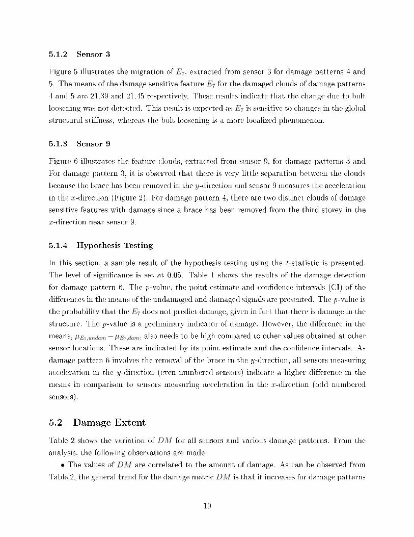
5.1.3 Sensor 9
Figure 6 illustrates the feature clouds, extracted from sensor 9, for damage patterns 3 and
For damage pattern 3, it is observed that there is very little separation between the clouds
because the brace has been removed in the y-direction and sensor 9 measures the acceleration
in the x-direction (Figure 2). For damage pattern 4, there are two distinct clouds of damage
sensitive features with damage since a brace has been removed from the third storey in the
x-direction near sensor 9.
5.1.4 Hypothesis Testing
In this section, a sample result of the hypothesis testing using the t-statistic is presented.
The level of signi�cance is set at 0.05. Table 1 shows the results of the damage detection
for damage pattern 6. The p-value, the point estimate and con�dence intervals (CI) of the
di�erences in the means of the undamaged and damaged signals are presented. The p-value is
the probability that the E7 does not predict damage, given in fact that there is damage in the
structure. The p-value is a preliminary indicator of damage. However, the di�erence in the
means, µE7,undam−µE7,dam, also needs to be high compared to other values obtained at other
sensor locations. These are indicated by its point estimate and the con�dence intervals. As
damage pattern 6 involves the removal of the brace in the y-direction, all sensors measuring
acceleration in the y-direction (even numbered sensors) indicate a higher di�erence in the
means in comparison to sensors measuring acceleration in the x-direction (odd numbered
sensors).
5.2 Damage Extent
Table 2 shows the variation of DM for all sensors and various damage patterns. From the
analysis, the following observations are made
• The values of DM are correlated to the amount of damage. As can be observed from
Table 2, the general trend for the damage metric DM is that it increases for damage patterns
10

6, 3, 4, 5, 1 and 2, which corresponds to a progressive increase in damage.
• With regard to DP4 and DP5, there is no change in the values of the damage measure,
thus indicating that bolt loosening could not be detected.
5.3 E�ect of Noise
The e�ect of zero mean additive Gaussian white noise on the damage detection algorithm is
studied. The ratio of the root mean square (rms) value of the noise to the rms value of the
signal is de�ned as the noise to signal ratio, and is denoted as NSR. The NSR is varied from
0.05 to 0.15. The values of DM with these noise levels for sensor 2 are presented in Table
2. From the analysis, the following observations are made:
• The values of DM are correlated to the amount of damage. For damage patterns 3
and 4, there is very slight di�erence between these values since at sensor 2, DP 4 is
DP 3 + removal of a brace in a direction perpendicular to the direction of acceleration
measured at sensor 2. Similar conclusions can be made for DP 4 and DP 5.
• The values of DM are sensitive to noise and only major damage patterns 1 and 2 can
be detected at high ranges of noise levels.
• As expected, the separation of the clouds decreases with noise.
6 Conclusions
In this paper, a damage detection algorithm based on the Morlet wavelet transform of the
vibration signal is presented. The main advantage of wavelet decomposition over other time
series and spectral methods is that the signal in question can be localized in both time and
scale domains, thus allowing for modeling non-stationarity in the signal. An expression for
the energies of the Morlet wavelet coe�cients of a vibration signal at scale a, Ea is derived for
a multi-degree of freedom system. It is shown that Ea is a function of the modal parameters
through the mass normalized eigenvectors, natural frequencies and damping ratios of the
system. It is observed that the energy of the wavelet coe�cients at seventh dyadic scale E7
changes with the onset of damage and consequently chosen as the damage sensitive feature.
Subsequently, the damage decision is made by comparing the means of E7 before and after
damage. This is achieved using a t-test. The p-values and the con�dence intervals for the
di�erence in the means of the DSF before and after damage are reported. A damage measure
DM based on the Mahalanobis distance is described. This damage detection methodology
11

is tested on the analytical results of the ASCE Benchmark Structure. The results of the
application of this damage detection algorithm indicates that the algorithm is able to detect
the existence of all damage patterns in the ASCE Benchmark Structure at relatively high
levels of noise. However, at higher noise levels, minor damage patterns are not detected. The
reason for this might be because that the sensitivity of the loading at these scales might have
dominated the sensitivity of the damage on the damage sensitive feature. Thus, it would be
critical to perform normalization step of the damage diagnosis algorithm. The results also
indicate that the damage measure DM is correlated to the amount of damage. The values
of DM are also sensitive to noise and only major damage patterns 1 and 2 can be detected
at high ranges of noise levels.
This algorithm is particularly suitable for embedment at the sensor level since it involves
local signal processing for feature extraction and a hypothesis test for the damage decision.
The developed algorithm is (i) simple since intensive �nite element modeling and updating
is not required as is the case with conventional system identi�cation algorithms (ii) robust
since these algorithms are able to detect and quantify minor damage patterns and (iii)
computationally e�cient since this algorithm uses only processing of signals at the sensor
level and lead to signi�cant saving in time of computation.
References
[1] Farrar, C. R and Worden, K. (2007). �An introduction to structural health monitoring.�
Philosophical Transactions of the Royal Society A, 365, 303-315.
[2] Ghanem, R. and Romeo, F. (2000). �A wavelet based approach for identi�cation of linear
time varying dynamical systems.� Journal of Sound and Vibration, 234(5), 555-576.
[3] Hou, Z. K., Noori, M. and St. Amand, R. (2000). �Wavelet-based approach for structural
damage detection.� ASCE Journal of Engineering Mechanics, 126(7), 677-683.
[4] Johnson, E. A., Lam, H. F., Katafygiotis, L. S. and Beck, J. L. (2004). �Phase I IASC-
ASCE structural health monitoring benchmark problem using simulated data.� ASCE
Journal of Engineering Mechanics, 130(1), 3-15.
[5] Kijewski, T. and Kareem, A. (2003). �Wavelet transforms for system identi�cation: con-
siderations for civil engineering applications.� Computer-Aided Civil and Infrastructure
Engineering, 18, 341-357.
12

[6] Lynch, J. P., Sundararajan, A., Law, K. H., Kiremidjian, A. S. and Carryer, E. (2004).
�Embedding damage detection algorithms in a wireless sensing unit for attainment of
operational power e�ciency�, Smart Materials and Structures, 13 (4), 800�810.
[7] Maia, N. M. M and Silva, J. M. M. (1998). Theoretical and Experimental Modal Analysis,
Research Studies Press, Hertfordshire, England.
[8] Mallat, S. (1999), A Wavelet Tour of Signal Processing, Academic Press, New York.
[9] Nair, K. K., Kiremidjian, A. S. and Law, K. H. (2006). �Time series based damage de-
tection and localization algorithm with application to the ASCE benchmark structure.�
Journal of Sound and Vibration, 291 (2), 349-368.
[10] Nair, K. K. and Kiremidjian, A. S. (2007). �Time series based structural damage detec-
tion algorithm using Gaussian mixtures modeling.� ASME Journal of Dynamic Systems,
Measurement and Control, 129(3), 285-293.
[11] Nair, K. K. (2007). Damage Diagnosis Algorithms for Wireless Structural Health Moni-
toring, PhD Dissertation, Department of Civil and Environmental Engineering, Stanford
University.
[12] Nair, K. K. and Kiremidjian, A. S. (2009). �Derivation of a Damage Sensitive Feature
using the Haar Wavelet Transform�, Forthcoming in the ASME Journal of Applied
Mechanics.
[13] Rice, J. A. (1999). Mathematical Statistics and Data Analysis, 2nd ed., Duxbury Press.
[14] Rytter, A. (1993). Vibration Based Inspection of Civil Engineering Structures. PhD
Dissertation, Department of Building Technology and Structural Engineering, Aalborg
University, Denmark.
[15] Sohn, H., Farrar, C. R., Hunter, H. F. & Worden, K. (2001). Applying the LANL
Statistical Pattern Recognition Paradigm for Structural Health Monitoring to Data from
a Surface E�ect Fast Patrol Boat. Los Alamos National Laboratory Report LA-13761-
MS, Los Alamos National Laboratory, Los Alamos, NM 87545.
[16] Staszewski, W. J. (2000). �Identi�cation of non-linear systems using multi-scale ridges
and skeletons of the wavelet transform,� Journal of Sound and Vibration, 214(4), 639-
658.
13

[17] Straser, E. and Kiremidjian, A. S. (1998). Modular Wireless Damage Monitoring Sys-
tem for Structures, Report No. 128, John A. Blume Earthquake Engineering Center,
Department of Civil and Environmental Engineering, Stanford University, Stanford,
CA, 1998.
[18] Sun, Z. and Chang, C. C. (2004). �Statistical wavelet based method for structural health
monitoring.� ASCE Journal of Structural Engineering, 130(7), 1055-1062.
14

Figures
Figure 1: Morlet Wavelet (a) Basis Function and (b) its Fourier Transform
15

Figure 2: Placement of sensors and directions of acceleration measurements on the ASCEBenchmark Structure (Johnson et al., 2004)
16

Figure 3: Migration of the Morlet wavelet based damage sensitive feature E7 for sensor 2with damage for minor patterns (a) Damage pattern 6 and (b) Damage Pattern 3
17

Figure 4: Migration of Morlet wavelet based damage sensitive feature E7 for sensor 2 withdamage for major patterns (a) Damage pattern 1 and (b) Damage Pattern 2
18

Figure 5: Migration of Morlet wavelet based damage sensitive feature E7 for sensor 3 withdamage for (a) Damage pattern 4 and (b) Damage Pattern 5
19

Figure 6: Migration of Morlet wavelet based damage sensitive feature E7 for sensor 9 withdamage for (a) Damage pattern 3 and (b) Damage Pattern 4
20

Tables
Sensor No. Damage Decision p-value Point Estimate CI of µE7,undam − µE7,dam
1 H1 8.21× 10⁻⁴ -0.13 [-0.21, -0.06]2 H1 4.41× 10⁻¹⁶ 2.70 [2.11, 3.29]3 H1 0.0021 0.17 [0.06, 0.28]4 H1 1.65× 10⁻¹² 2.67 [1.98, 3.35]5 H1 0.0045 -0.31 [-0.52, -0.09]6 H1 4.22× 10⁻¹⁵ 4.51 [3.48, 5.53]7 H1 0.0086 0.28 [0.07, 0.48]8 H1 4.55× 10⁻¹⁰ 3.07 [2.16, 3.99]9 H0 0.087 -0.31 [-0.67, 0.05]10 H1 2.47× 10⁻¹¹ 5.00 [3.63, 6.38]11 H0 0.11 0.34 [-0.07, 0.75]12 H1 1.06× 10⁻¹⁰ 4.58 [3.28, 5.89]13 H0 0.0676 -0.37 [-0.77, 0.03]14 H1 8.15× 10⁻¹³ 4.43 [3.31 5.56]15 H0 0.11 0.28 [-0.06, 0.63]16 H1 1.48× 10⁻⁷ 3.45 [2.21, 4.68]
Table 1: Results of the damage detection algorithm for damage pattern 6
21

Sensor No. Damage Pattern
DP1 DP2 DP3 DP4 DP5 DP6
1 9.68 21.52 0.85 0.95 0.95 0.332 99.63 146.00 7.71 7.49 7.49 1.633 9.12 18.43 0.98 2.57 2.57 0.354 97.10 123.32 5.89 5.58 5.58 1.335 5.85 10.96 1.27 1.49 1.49 0.396 62.01 72.05 6.70 6.60 6.60 1.467 7.13 12.65 1.87 2.13 2.13 0.398 63.94 80.00 4.66 4.55 4.55 1.089 6.18 11.35 0.95 6.65 6.65 0.2510 50.89 43.29 5.46 5.49 5.49 1.5211 5.54 9.51 1.22 5.49 5.49 0.2512 53.05 43.02 5.02 5.06 5.06 1.1113 3.12 8.12 0.97 1.60 1.60 0.2714 48.64 43.83 5.74 5.52 5.52 1.2915 4.53 10.89 1.06 1.48 1.48 0.2416 40.76 41.20 3.87 3.90 3.90 0.88
Table 2: Variation of DM for the Morlet wavelet based damage sensitive feature for varioussensors and di�erent damage patterns
22

NSR Damage Patterns
DP 1 DP 2 DP 3 DP 4 DP 5 DP 6
0.0 99.63 146.00 7.71 7.49 7.49 1.630.5 57.00 78.17 2.11 1.84 1.84 0.360.10 20.11 35.16 0.88 0.53 0.53 0.000.15 10.49 17.13 0.22 0.46 0.46 0.00
Table 3: Variation of DM for sensor 2 with di�erent noise to signal ratios (NSR) for damagepatterns DP 1-6
23