a data-driven epidemiological prediction method for dengue ... · a data-driven epidemiological...

Buczak et al. BMC Medical Informatics and Decision Making 2012, 12:124http://www.biomedcentral.com/1472-6947/12/124

RESEARCH ARTICLE Open Access

A data-driven epidemiological prediction methodfor dengue outbreaks using local and remotesensing dataAnna L Buczak*, Phillip T Koshute, Steven M Babin, Brian H Feighner and Sheryl H Lewis

Abstract

Background: Dengue is the most common arboviral disease of humans, with more than one third of the world’spopulation at risk. Accurate prediction of dengue outbreaks may lead to public health interventions that mitigatethe effect of the disease. Predicting infectious disease outbreaks is a challenging task; truly predictive methods arestill in their infancy.

Methods: We describe a novel prediction method utilizing Fuzzy Association Rule Mining to extract relationshipsbetween clinical, meteorological, climatic, and socio-political data from Peru. These relationships are in the form ofrules. The best set of rules is automatically chosen and forms a classifier. That classifier is then used to predict futuredengue incidence as either HIGH (outbreak) or LOW (no outbreak), where these values are defined as being aboveand below the mean previous dengue incidence plus two standard deviations, respectively.

Results: Our automated method built three different fuzzy association rule models. Using the first two weeklymodels, we predicted dengue incidence three and four weeks in advance, respectively. The third predictionencompassed a four-week period, specifically four to seven weeks from time of prediction. Using previously unusedtest data for the period 4–7 weeks from time of prediction yielded a positive predictive value of 0.686, a negativepredictive value of 0.976, a sensitivity of 0.615, and a specificity of 0.982.

Conclusions: We have developed a novel approach for dengue outbreak prediction. The method is general, couldbe extended for use in any geographical region, and has the potential to be extended to other environmentallyinfluenced infections. The variables used in our method are widely available for most, if not all countries, enhancingthe generalizability of our method.

Keywords: Dengue fever, Prediction, Association rule mining, Fuzzy logic, Predictor variables

BackgroundDengue is an acute febrile disease of humans caused bya single-stranded RNA flavivirus transmitted by Aedesmosquitoes, primarily Aedes aegypti. These mosquitoesthrive in tropical urban areas by breeding in uncoveredcontainers capable of holding rain water, such as tires,buckets, flower pots, etc. [1]. Dengue is now the mostcommon arboviral disease of humans in the world [2,3],recognized in over 100 countries, with an estimated50 – 100 million cases annually [4,5]. More than one thirdof the world’s population lives in the areas where there is a

* Correspondence: [email protected] Hopkins University Applied Physics Laboratory, 11100 Johns HopkinsRd, Laurel, MD 20723-6099, USA

© 2012 Buczak et al.; licensee BioMed CentralCommons Attribution License (http://creativecreproduction in any medium, provided the or

risk of dengue virus transmission. Recent dengue out-breaks have occurred in the Philippines, Singapore,Thailand, Cambodia, Peru, Ecuador, and Brazil [6]. Den-gue is endemic in Puerto Rico and recently re-emerged inthe Florida Keys in the United States (US) [7].Dengue presents with a wide range of symptoms [2].

Minimally symptomatic or mild flu-like presentationsmay be seen in young children. The classic presentation(called dengue fever or DF), seen most commonly inolder children and adults, is an abrupt onset of a highfever, severe muscle and joint pain, and headache thatmay occur with nausea and vomiting. Recovery is pro-longed and marked by fatigue and depression [8]. Ahemorrhagic form of the disease may develop, especially

Ltd. This is an Open Access article distributed under the terms of the Creativeommons.org/licenses/by/2.0), which permits unrestricted use, distribution, andiginal work is properly cited.

mailto:[email protected]

http://creativecommons.org/licenses/by/2.0

Buczak et al. BMC Medical Informatics and Decision Making 2012, 12:124 of 20http://www.biomedcentral.com/1472-6947/12/124

in patients who have been exposed to more than one ofthe four known strains of the virus [2,6]. This presenta-tion, called dengue hemorrhagic fever (DHF), includesincreased capillary permeability with potentially signifi-cant vascular leakage that compromises organ functionand may lead to shock [2-4]. Mortality in DHF with ex-cellent medical care is generally less than 10%, but hasbeen reported to be as high as 40% in austere settings [2].Efforts to develop a dengue vaccine have been ham-

pered by lack of appropriate animal models. Additionally,the empirical observation of increased incidence of DHFwith prior immunologic response to dengue virus infec-tion raises the theoretical possibility that immunizationmay result in an increased incidence of DHF [9]. Severaldengue vaccines are currently undergoing clinical trials;however, no dengue vaccine is licensed for use in the US.Therefore, it is important to find ways to accurately pre-dict dengue outbreaks in order that preventive publichealth interventions may be used to mitigate the effect ofthese outbreaks, particularly in areas where resources forsuch efforts are limited and where medical treatment fa-cilities may become overwhelmed by an outbreak.

MethodsPredictor variablesPrevious investigators have described dengue predictivemodels using a variety of different input variables[10-19]. Because of characteristics of vector transmission,pre-outbreak dengue incidence rate [1] and seropreva-lence [20] reflect the presence of the virus in the humanpopulation and are expected to be good indicators ofoutbreak potential. Temperature is also often used be-cause of its effects on biological parameters such as theextrinsic incubation period of the mosquito [1,21]. As themosquito vector requires water for completion of its lifecycle, investigators have examined the use of rainfalldata for disease outbreak prediction [1]. These rainfalldata may be locally acquired or derived via satellitemeasurements. The Tropical Rainfall Measuring Mission(TRMM) satellite data have been used to derive rainfallmeasurements [22] in remote and resource-limitedregions and these measurements have been used for pre-dictions for disease outbreaks [23]. In addition, satellitemeasurements of leaf area indices have been used to as-sess green leaf biomass, photosynthetic activity, and theeffects of seasonal rainfall, which are then related tovector habitat characteristics and disease outbreaks [24].Commonly used leaf area indices are the Normalized Dif-ference Vegetation Index (NDVI) and the EnhancedVegetation Index (EVI), both available from satellite sen-sors such as the Advanced Very High Resolution Radi-ometer (AVHRR) and the Moderate Resolution ImagingSpectrometer (MODIS). NDVI is closely related tophotosynthesis, while EVI is closely related to leaf

display [22]. Because climate effects, such as the El NinoSouthern Oscillation (ENSO), can indicate near-term fu-ture rainfall anomalies, the Southern Oscillation Index(SOI) and various sea surface temperature anomalies(SSTA) have also been used as indicators of future dis-ease outbreaks [10,25-27]. Our method uses variablessuch as previous dengue incidence, meteorological/climaticdata (rainfall, day temperature, night temperature, NDVI,EVI, SSTA, SOI), and socio-economic data (political stabil-ity, sanitation, water, and electricity). Sources of these datacan be found in Table 1.In order to perform spatiotemporal predictions, all the

variables need to fit the same spatiotemporal scale. Thespatiotemporal scale used in this work was selectedbased on the distribution of the dengue data: the chosentemporal scale was one week and the chosen spatial dis-tribution was one district. In the following sections,when describing the different variables used, we also de-scribe the extensive preprocessing done for each variableto fit the selected spatiotemporal scale.

Dengue case dataWe obtained dengue case data from our collaborators atthe Peruvian Ministry of Health. We took into accountcases marked as “probable” and “confirmed” and did notinclude cases labeled “discarded.” Information for eachcase included year, week number (within a year), anddistrict. With this information, cases per week in a givendistrict could be counted (Figure 1). The data setincluded dengue case data from 2001–2009.The province of Loreto, from which we had these data,

consists of 51 districts. In this study, we considered onlysix of those districts (see Figure 2) that had a large num-ber of dengue cases (Belen, Fernando Lores, Iquitos,Punchana, San Juan Bautista, and Yurimaguas).For a given district, we calculated dengue incidence

per week per 1000 residents (Figure 3):

Incidenceweek ¼ ♯casesweek � 1000=populationweek

In the calculations, we assumed that the population ofa district was constant throughout a given year. To de-rive these population values, we obtained district popu-lation data from Peru National Institute of Statistics andInformation from the 1993 and 2007 censuses (therewas no census taken in between these years). For eachdistrict, we used a linear interpolation to obtain thepopulation for each of the years between 1993 and 2007,and we used a linear extrapolation to obtain the popula-tion for 2008 and 2009. When portions of Iquitos werereassigned to Belen and San Juan Bautista in 2000, weassumed that the three districts’ total populationincreased linearly and that the ratio between themremained constant.

Table 1 Sources of data

Data type Source

Rainfall NASA Tropical Rainfall Measuring Mission http://mirador.gsfc.nasa.gov/

Temperature USGS Land Processes Distributed Active Archive Center https://lpdaac.usgs.gov/get_data

Altitude NOAA National Geophysical Data Center http://www.ngdc.noaa.gov/cgi-bin/mgg/ff/nph-newform.pl/mgg/topo/.

Demographics Peru National Institute of Statistics and Information http://www.inei.gob.pe/

NDVI USGS Land Processes Distributed Active Archive Center https://lpdaac.usgs.gov/get_data

EVI USGS Land Processes Distributed Active Archive Center https://lpdaac.usgs.gov/get_data

Political Stability Worldwide Governance Indicators Project http://info.worldbank.org/governance/wgi/index.asp

Southern Oscillation Index US National Center for Atmospheric Research http://mirador.gsfc.nasa.gov/

Sea Surf. Temp. Anomaly NASA Global Change Mastery Directory https://lpdaac.usgs.gov/get_data


For subsequent analysis, we aggregated weekly inci-dence values into four-week interval values (Figure 4),by adding the individual weeks’ incidence values. Specif-ically, the incidence for the interval from week i to weeki + 3 can be obtained with:

Incidencei�iþ3 ¼ Incidencei þ Incidenceiþ1

þ Incidenceiþ2 þ Incidenceiþ3

Because dengue cases were provided in weekly intervals,we converted all other input variables to weekly intervals.Following US Centers for Disease Control and Prevention(CDC) conventions [28], all weekly intervals begin on aSunday.

RainfallRainfall data with 0.25-degree resolution were obtainedfrom the satellite measurements of the NASA TropicalRainfall Measuring Mission (TRMM). After downloading

Figure 1 Dengue cases per week.

data from the TRMM website [29] in hierarchical data for-mat (HDF), we used MATLAB [30], tools to extract therelevant data layers. These data contained hourly rainfallrates, averaged over three-hour intervals. To convert fromrainfall rates to rainfall amounts, we multiplied all data bythree (the number of hours in the measurement interval).We then aggregated the resulting data into daily andweekly totals. Following CDC convention [28], we definedall weeks to begin on a Sunday. Figure 5 shows an ex-ample of rainfall amounts for a single day. In the data set,some data were missing so we assigned rainfall totals ofzero for each of these instances.Spatial aggregation of rainfall data from 0.25 degree

grid cells to districts was performed by first computing aweight equivalent to estimated proportions of a districtcomprised by each grid cell. We then used each district’sset of weights and the gridded rainfall values for a givenweek, to determine a single rainfall amount for each

http://www.inei.gob.pe/

https://lpdaac.usgs.gov/get_data


http://info.worldbank.org/governance/wgi/index.asp

http://mirador.gsfc.nasa.gov/


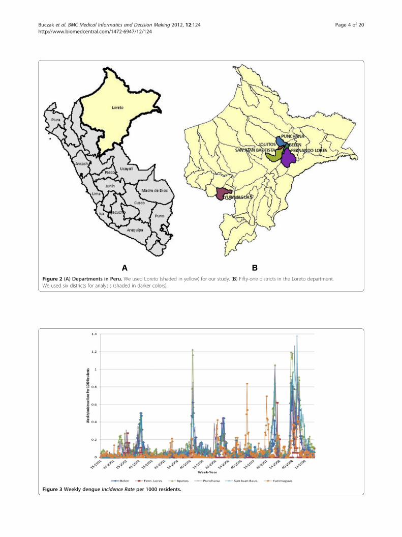
A BFigure 2 (A) Departments in Peru. We used Loreto (shaded in yellow) for our study. (B) Fifty-one districts in the Loreto department.We used six districts for analysis (shaded in darker colors).

Figure 3 Weekly dengue Incidence Rate per 1000 residents.


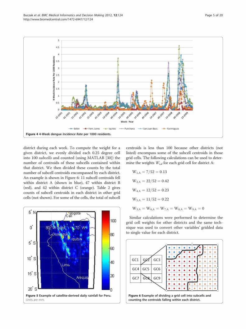
Figure 4 4-Week dengue Incidence Rate per 1000 residents.


district during each week. To compute the weight for agiven district, we evenly divided each 0.25 degree cellinto 100 subcells and counted (using MATLAB [30]) thenumber of centroids of these subcells contained withinthat district. We then divided these counts by the totalnumber of subcell centroids encompassed by each district.An example is shown in Figure 6: 11 subcell centroids fellwithin district A (shown in blue), 47 within district B(red), and 42 within district C (orange). Table 2 givescounts of subcell centroids in each district in other gridcells (not shown). For some of the cells, the total of subcell

Figure 5 Example of satellite-derived daily rainfall for Peru.Units are mm.

centroids is less than 100 because other districts (notlisted) encompass some of the subcell centroids in thosegrid cells. The following calculations can be used to deter-mine the weights Wi,d for each grid cell for district A:

W1;A ¼ 7=52 ¼ 0:13

W2;A ¼ 22=52 ¼ 0:42

W4;A ¼ 12=52 ¼ 0:23

W5;A ¼ 11=52 ¼ 0:22

W3;A ¼ W6;A ¼ W7;A ¼ W8;A ¼ W9;A ¼ 0

Similar calculations were performed to determine thegrid cell weights for other districts and the same tech-nique was used to convert other variables’ gridded datato single value for each district.

Figure 6 Example of dividing a grid cell into subcells andcounting the centroids falling within each district.

Table 2 Numbers of subcell centroids from each grid cellin districts A, B, and C. GC stands for Grid Cell

District GC1 GC2 GC3 GC4 GC5 GC6 GC7 GC8 GC9

A 7 22 0 12 11 0 0 0 0

B 0 2 0 67 47 0 18 13 0

C 0 5 15 0 42 34 0 65 25


For subsequent analysis, we aggregated weekly rainfallvalues into four-week interval values, by adding the indi-vidual weeks’ rainfall values. Specifically, the rainfall forthe interval from week i to week i + 3 can be obtainedwith:

Rainfalli�iþ3 ¼ Rainfalli þ Rainfalliþ1 þ Rainfalliþ2

þ Rainfalliþ3

TemperatureWe obtained eight-day interval temperature meanswith 0.05 degree resolution from the United StatesGeological Survey (USGS) Land Processes DistributedActive Archive Center. After downloading the datafrom their website [31] in HDF file format, we usedMATLAB [30] tools to extract the relevant data layers.We considered and identically processed both daytimeand nighttime temperatures. An example of daytimetemperature values for a given 8-day interval areshown in Figure 7.

Figure 7 Example of day-time temperature data for a given8-day interval. Units are degrees Celsius. Procedures weredeveloped in MATLAB to remove missing data. The dark blue spotsnear Iquitos (corresponding to a temperature near 0 C) wereremoved since they were corresponding to missing data.

We converted the temperature data from 0.05 degreeto 0.25 degree resolution in order to match the reso-lution of the rainfall data (shown in Figure 8). Generally,we aggregated the data into the quarter-degree cells byaveraging the 25 smaller cells’ values. But where some ofthe data were missing, we only included the grid cellswith actual data. If all temperature values were missingfor an entire 0.25 degree grid cell, we set thetemperature value for that grid cell to “missing”.Subsequently, we calculated single-week averages from

eight-day means, coincident with weekly dengue inci-dence data. In some cases, an entire week was containedwith an 8-day interval and we set the temperature forthat week to the means from that 8-day interval. Inother cases, we used weighted sums of the means of ad-jacent 8-day intervals. Specifically, we applied:

Tweek ¼ T8;i di=7ð Þ þ T8;iþ1 diþ1=7ð Þ

where di is the number of days in the week overlappingthe ith 8-day interval and T8,i is the temperature in that8-day interval.In cases where one of two 8-day intervals had missing

data from a given grid cell, we used the mean from theother 8-day interval exclusively. In cells where all valuesfrom corresponding 8-day intervals were “missing” data,we excluded these temperature values from the subse-quent spatial aggregation whenever possible. (In a smallnumber of cases, all temperature data from all grid cellscomprising a given district were missing for an entireweek and we set that district’s temperature to “missing”).To determine grid cell weights for each district, we ap-plied the subcell centroid counting method (describedearlier in the section entitled Rainfall) that we used todetermine grid cell weights for rainfall.For subsequent analysis, we aggregated weekly tem-

perature values into four-week interval values, by takingthe average of the individual weeks’ temperature values.

Figure 8 Illustration of spatial resolution of different variables.


Specifically, the temperature for the interval from week ito week i + 3 can be obtained with:

Temperatureiiþ3 ¼ Temperaturei þ Temperatureiþ1ðþTemperatureiþ2 þ Tempeartureiþ3Þ=4

Vegetation indices: NDVI and EVIWe obtained 16-day interval Normalized DifferenceVegetation Index (NDVI) values and Enhanced Vegeta-tion Index (EVI) values with 0.05 degree resolution fromthe USGS Land Processes Distributed Active ArchiveCenter [31]. Examples of NDVI and EVI data are shownin Figures 9 and Figure 10, respectively.These data consist of satellite measurements of leaf

area indices that provide a surrogate assessment of greenleaf biomass, photosynthetic activity, and the effects ofseasonal rainfall, which may then be related to vectorhabitat characteristics and disease outbreaks [32]. NDVIis closely related to photosynthesis, while EVI is closelyrelated to leaf display [33]. Values of both NDVI andEVI were obtained from the Moderate Resolution Im-aging Spectrometer (MODIS).Negative values (approaching −1) of NDVI correspond

to water. Values close to zero (−0.1 to 0.1) correspond tobarren areas of rock, sand, or snow. Low positive values(approximately 0.2 to 0.4) represent shrub and grassland.High values (approaching 1) indicate temperate and trop-ical rainforests. NDVI seasonal variations closely followhuman-induced patterns, resulting in a significant correl-ation between NDVI and landscape disturbance [33].EVI is an optimized index designed to enhance the

vegetation signal with improved sensitivity in high bio-mass regions and improved vegetation monitoring

Figure 9 Example of NDVI values for a given 16-day interval.

through a decoupling of the canopy background signaland a reduction in atmosphere influences. EVI is calcu-lated similarly to NDVI, but corrects for some distor-tions in the reflected light. EVI is considered to be moreresponsive than NDVI to canopy structural variations.Xiao et al. [34] note that the fact that EVI includes theblue band for atmospheric correction is particularly im-portant for the Amazon basin where seasonal burning ofpasture and forest takes place throughout the dry sea-son. They note that, unlike EVI, NDVI could be substan-tially impacted by the smoke and aerosols from biomassburning, regardless of the vegetation changes.For NDVI and EVI, we used data processing steps

similar to that of temperature: downloading in HDF for-mat from the USGS LPDAAC website [31], extractingrelevant data layers with MATLAB [30] tools, convertingfrom 0.05 degree to 0.25 degree resolution, and account-ing for missing data. Subsequently, we combined 16-daymeans to obtain single-week averages, coincident withweekly dengue incidence. In some cases, an entire weekwas contained with a 16-day interval and we set theNDVI and EVI values for that week to the values fromthat 16-day interval. In other cases, we used weightedsums of the values of adjacent 16-day intervals. Specific-ally, we applied:

Nweek ¼ N16;i di=7ð Þ þ N16;iþ1 diþ1=7ð Þ

where di is the number of days in the week overlappingthe ith 16-day interval and N16,i is the NDVI or EVIvalue for that 16-day interval.In cases where one of two 16-day intervals was miss-

ing data from a given grid cell, we used the value fromthe other 16-day interval exclusively. In cells where all

Figure 10 Example of EVI values for a given 16-day interval.


values from corresponding 16-day intervals were missingdata, we excluded these NDVI and EVI values from thesubsequent spatial aggregation. To assign single NDVI/EVI values for each district, we applied the subcell cen-troid counting method described earlier in the sectionentitled Rainfall.For subsequent analysis, we aggregated weekly NDVI/

EVI values into four-week interval values, by taking theaverage of the individual weeks’ NDVI/EVI values. Spe-cifically, the NDVI/EVI for the interval from week i toweek i + 3 can be obtained with:

Indexiiþ3 ¼ Indexi þ Indexiþ1 þ Indexiþ2 þ Indexiþ3ð Þ=4where Index stands for NDVI or EVI depending forwhich one the calculation is being performed.

Southern Oscillation IndexWe obtained monthly Southern Oscillation Index (SOI)values from the US National Center for Atmospheric Re-search Climate Analysis Section website [35]. SOI isbased on the pressure difference between Darwin(Australia) and Tahiti (French Polynesia), which influ-ences the strength of the prevailing easterly winds. Thesedata provide a measure of the El Nino Southern Oscilla-tion (ENSO) climate effect. A single monthly SOI valueis available and therefore is not location-specific.We processed monthly SOI values to obtain single-

week values, coincident with weekly dengue data. Inmost cases, an entire week was contained with a givenmonth and we set the SOI values for that week to thevalue from the encompassing month. In other cases, weused weighted sums of the values of adjacent month.Specifically, we applied:

Sweek ¼ Sm;i di=7ð Þ þ Sm;iþ1 diþ1=7ð Þwhere di is the number of days in the week overlappingthe ith month and Sm,i is the SOI for that month.

Sea Surface Temperature AnomalyAs a complement to SOI values, we obtained weekly SeaSurface Temperature Anomaly (SSTA) values from theNASA Global Change Mastery Directory website [36].Different SSTA values are computed for different regionsof the Pacific Ocean and we used the SSTA values forthe regions directly adjacent to Peru (Nino regions 1 and2). Unlike SOI, SSTA values are typically published for asingle week, beginning on Wednesday. To align thesevalues with weekly dengue data (beginning on Sunday),we computed weighted sums according to

Aweek ¼ Aw;i di=7ð Þ þ Aw; diþ1=7ð Þwhere di is the number of days in the week overlappingthe ith week and Aw,i is the SSTA for that week.

Socio-economic and demographic dataWe considered several socio-economic variables thatreflected potentially relevant information. We obtainedpolitical stability data from the Worldwide GovernanceIndicators Project [37]. These data consisted of a singlevalue for Peru from most years between 1996 and 2009.To obtain values for the missing years, we performed alinear interpolation. From the Peru National Institute ofStatistics and Information 2007 census [38], we obtainedpopulation density and proportions with electric light-ing, running water, and hygienic services. These dataalso included numbers of vivendas particulares (privatedwellings), vivendas con abstecimiento de agua (privatedwellings with running water), vivendas con serviciohigienico (private dwellings with toilets), and vivendascon alumbrado electric (private dwellings with electricity)for each district. We then calculated percentages of privatedwellings with running water, toilets, and electricity. Be-cause these values were only available from the 2007 cen-sus, we used a single value for each district for all weeks.

ElevationWe obtained elevation data from the NOAA NationalGeophysical Data Center website [39]. We assignedmissing data (typically for ocean locations) an elevationof zero. By averaging the elevation in 30-by-30 grids, wechanged the scale from 1/120 degree to 0.25 degreeresolution, consistent with the scale of rainfall data. Sub-sequently, we used the subcell centroid counting method(described earlier in the section entitled Rainfall) to de-termine a single average elevation value for each district.

Prediction methodologyOverviewThe dengue prediction methodology developed has thefollowing steps (Figure 11):

1 Definition of spatiotemporal resolution and datapreprocessing to fit that resolution.

2 Division of the data set into disjoint training,validation and test subsets.

3 Rule extraction from training data using FuzzyAssociation Rule Mining (FARM).

4 Automatic building of classifiers from the rulesextracted in step 3.

5 Choice of the best classifier based on its performanceon the validation data set.

6 Computation of predictions on the test data using theclassifier from step 5. Computation of performancemetrics.

Because different model input data come in disparatespatiotemporal scales, they were converted to one spa-tiotemporal scale to be used in the prediction method.

Figure 11 Dengue prediction method developed.


The chosen temporal scale was one week and the chosenspatial distribution was one district. In step 1 all the pre-dictor and epidemiological data were converted into thisspatiotemporal scale. Details of this conversion weredescribed earlier in the section entitled Predictorvariables.The second step was to divide the data set into disjoint

training, validation and test subsets. FARM [40] wasused on the training subset in step 3 to extract rules pre-dicting future dengue incidence (details described laterin the section entitled Association rule mining andfuzzy association rule mining). Step 4 involved theautomatic building of classifiers from rules extracted instep 3. A separate, validation subset was used to choosethe best performing classifier in step 5. Finally, in step 6,a third data subset was used to predict the dengue inci-dence and determine the accuracy of the method.Rule extraction from the training data (step 3) is the

most important and novel step of the whole methodology.It is performed using FARM, a set of data mining methodsthat automatically extract from data so-called fuzzy associ-ation rules [41]. Fuzzy association rules are of the form:IF (X is A) → (Y is B).

where X and Y are variables, and A and B are fuzzysets that characterize X and Y respectively. The follow-ing is a simple example of a fuzzy association rule (notactually used in the method):IF (Temperature is HOT) AND (Humidity is HIGH) →

(Energy usage is HIGH).Fuzzy association rules are easily understood by

humans because of the linguistic terms that they employ(e.g., HOT, HIGH). Fuzzy set theory [42] assigns a de-gree of membership between 0 and 1 (e.g., 0.4) to eachelement of a set, allowing for a smooth transition be-tween full membership (degree=1) and non-membership(degree=0). The degree of membership in a set is gener-ally considered to be the extent to which a correspond-ing fuzzy set applies. For example, if the variable istemperature and the linguistic term (fuzzy set) is HOTthen you might consider a temperature of 70F to have adegree of membership of 0.1 in the fuzzy set HOT, whilea temperature of 80F might have a membership degreeof 0.8 and a temperature of 100F might have member-ship degree equal to 1.FARM extracts a large number of rules (possibly hun-

dreds or even thousands) from a training data set. When


the classifier is automatically built from those rules, therules have only one consequent, which is the variable tobe predicted (i.e., future dengue incidence). When build-ing a classifier, a subset of rules must be chosen; the sub-set chosen is the one that results in a smallestmisclassification error for the validation set. For buildingthe classifier, we have extended the method of Liu et al.[43] as will be described in the section entitled Buildingthe classifier. There are certain class weights that needto be assigned and the final classifier is the one that hasthe lowest misclassification error on the validation set.The final step was the computation of predictions by

the classifier. The outcome variable (predicted dengueincidence) was converted to a binary variable, eitherHIGH or LOW dengue incidence (where the thresholdbetween high and low values is quantitatively defined inFARM-based methods results section as the mean den-gue incidence + 2 standard deviations). Testing was per-formed on the test data and the following performancemetrics were used to assess the accuracy of this predic-tion: Positive Predictive Value (PPV), Negative PredictiveValue (NPV), sensitivity, and specificity. PPV is the pro-portion of dengue outbreaks that are correctly identified,while NPV is the proportion of periods without out-breaks that are correctly identified.

Details of the prediction methodology

Association rule mining and fuzzy association rulemining The goal of data mining is to discover inherentand previously unknown information from data. Whenthe knowledge discovered is in the form of associationrules, the methodology is called association rule mining(ARM). An association rule describes a relationshipamong different attributes. Association rule mining wasintroduced by Agrawal et al. [44] as a way to discoverinteresting co-occurrences in supermarket data (themarket basket analysis problem). It finds frequent sets ofitems (i.e., combinations of items that are purchased to-gether in at least N transactions in the database), andfrom the frequent items sets such as {X, Y}, generates as-sociation rules of the form: X → Y and/or Y → X. Asimple example of an association rule pertaining to theitems that people buy together is:IF (Bread AND Butter) → MilkThe above rule states that if a person buys bread and

butter, then they also buy milk. Such rules are very use-ful for store managers to help decide how to group itemson the shelves. Many extracted rules are obvious, as theone mentioned above. However ARM methods extractnot only well known rules but, more importantly,novel rules unknown to Subject Matter Experts (SMEs).Those rules are often surprising to SMEs as the nowfamous rule:

IF Diapers → Beer.The store managers did not want to believe that there

was a relationship between buying diapers and buyingbeer and thought that the ARM methodology thatextracted that rule from data was flawed. However aftercarefully checking the store transactions, they noticedthat in the evenings this rule was very prominent: whensomebody was buying diapers they were also buyingbeer. After further investigation, they concluded that inthe afternoons/evenings, moms often ask dads to buysome diapers; dads do that and reward themselves bybuying beer.A limitation of traditional association rule mining is

that it only works on binary data (i.e., an item was eitherpurchased in a transaction (1) or not (0)). In many real-world applications, data is either categorical (e.g., districtname, type of public health intervention) or quantitative(e.g., rainfall, temperature, age). For numerical and cat-egorical attributes, Boolean rules are unsatisfactory.Extensions have been proposed to operate on these data,such as quantitative association rule mining [45] andfuzzy association rule mining [41].Fuzzy association rules are of the form:IF (X is A) → (Y is B).where X and Y are variables, and A and B are fuzzy

sets that characterize X and Y respectively. A simple ex-ample of fuzzy association rule for a medical applicationis the following:IF (Temperature is Strong Fever) AND (Skin is

Yellowish) AND (Loss of appetite is Profound) →(Hepatitis is Acute).The rule states that if a person has a Strong Fever,

Yellowish skin and Profound Loss of appetite, then theperson has Acute Hepatitis. Strong Fever, Yellowish, Pro-found and Acute are membership functions of the vari-ables Temperature, Skin, Loss of appetite and Hepatitis,respectively. As an example of fuzzy membership func-tions, the membership functions for the variableTemperature are shown in Figure 12. According to thedefinition in that figure a person with a 100F Temperaturehas a Normal temperature with a membership value of0.2 and has a Fever with a membership value of 0.78.More information on Fuzzy Logic and fuzzy membershipfunctions can be found in [42].More formally, let D = {t1, t2, . . ., tn} be the trans-

action database and let ti represent the ith transactionin D. Let I={i1, i2,. . . im} be the universe of items. Aset X� I of items is called an itemset. When X has kelements, it is called a k-itemset. An association ruleis an implication of the form X → Y, where X ⊂ I,Y ⊂ I and X \ Y = φ.ARM and FARM rules have certain metrics associated

with them. The three metrics most widely used are Sup-port, Confidence and Lift and we will be using these

Figure 12 Membership functions for the fuzzy variable Temperature: Low, Normal, Fever, Strong Fever and Hyperthermia.


metrics in the method’s development. The support of anitemset X is defined as:

Support Xð Þ ¼ number records with Xnumber records in D

¼ nxn

¼ px

where n is the number of records in D, nx is the numberof records with X, and px is the associated probability.The support of a rule (X → Y) is defined as:

Support X→Yð Þ ¼ number records with X and Ynumber records in D

¼ nxyn

¼ pxy

where nxy is the number of records with X and Y, andpxy is the associated probability.The confidence of a rule (X → Y) is defined as:

Confidence X→Yð Þ ¼ number records with X and Ynumber records with X

¼ nxynx

¼ nxyn

� nnx

¼ pxypx

Confidence can be treated as the conditional probabil-ity (P(Y|X)) of a transaction containing X of also con-taining Y. A high confidence value suggests a strongassociation rule. However, this can be deceptive. For ex-ample, if the antecedent (X) or consequent (Y) have ahigh support, they could have a high confidence even ifthey were independent. This is why the measure of liftwas suggested as a useful metric.The lift of a rule (X → Y) measures the deviation from

independence of X and Y:

Lift X→Yð Þ ¼ Confidence X→Yð ÞSupport Yð Þ ¼ pxy

px� 1py

¼ pxypx � py

A lift greater than 1.0 indicates that transactionscontaining the antecedent (X) tend to contain the

consequent (Y) more often than transactions that do notcontain the antecedent (X). The higher the lift, the morelikely that the existence of X and Y together is not just arandom occurrence, but rather due to the relationshipbetween them.

Building the classifierFARM extracts a large set of rules from the trainingdata. For the disease prediction application, the rules ofinterest are called class association rules (CARs), mean-ing that they have only one consequent - the class. Anexample of a CAR extracted by FARM is:IF (Past_Incidence_Rate_T-1 is HIGH) AND (Past_In-

cidence_Rate_T-5 is HIGH) AND (Rainfall_T-3 isLARGE) → (Predicted_Incidence_Rate_T+4 is HIGH),confidence = 0.95, support = 0.01, lift = 5.3.The question is which rules from the hundreds

extracted by FARM to use in the final classifier and inwhich sequence to use them. When building the classi-fier, we first employed the method of Liu et al. [43]. LetR be the set of generated rules and D be the trainingdata. The basic idea of the algorithm is to choose a subsetof rules from R to cover all the training examples (D). Theclassifier will have the following format: <r1, r2, . . ., rm, de-fault class>. Default class is the one into which a case willbe classified, if none of the rules satisfies it. The order ofthe rules in the classifier is important and in classifying acase, the first rule that satisfies it will classify it.The algorithm has the following steps:

Step 1: Order the rules in R by:

1 Confidence (from highest to lowest);2 Support (from highest to lowest);3 Number of antecedents (from lowest to highest).


Step 2: Select the rules for the classifier from R. For agiven rule r, find cases in D that are covered by r (i.e.they satisfy the conditions of r). Remove from D thecases covered. Compute the number of errors that therule makes and add the rule to the classifier (C). A de-fault class is also selected – this is the majority class inthe remaining data in D. When there is no rule or notraining case left, then the rule selection process iscompleted.Step 3: Discard the rules from C that do not improve

the accuracy of the classifier.

The classifier generated by the algorithm above didnot have a satisfactory accuracy for dengue predictionand had the tendency to classify almost all of the casesinto the LOW category. The LOW category is a majoritycategory in the data and 94.5% of training data areLOW. This makes it much more challenging for theclassifier to learn to classify cases as HIGH. Thereforewe introduced the following changes to the classifierbuilding algorithm:

1 The rules are being ordered first by confidence, thenby lift, and finally by the number of antecedents.

2 The misclassification error is weighted. The user hasthe opportunity to give a much higher weight formisclassifying the cases that should be HIGH thanthose that should be LOW. We used 10 and 1,respectively.

ResultsFARM-based method resultsAn example rule extracted by FARM from the data is:IF (Past_Incidence_Rate_T-1 is HIGH) AND (Past_

Incidence_Rate_T-5 is HIGH) AND (Rainfall_T-3 isLARGE) → (Predicted_Incidence_Rate_T+4 is HIGH),confidence = 0.95

Table 3 Variables used

Weekly prediction: Prediction 3 weeks ahead Weekly prediction

Past Incidence Rate (T-12, T-11, . . ., T-1, T) Past Incidence Rate (

Rainfall (T-12, T-11, . . ., T-1, T) Rainfall (T-12, T-11, .

NDVI (T-12, T-11, . . ., T-1, T) NDVI (T-12, T-11, . . .,

SOI (T) SSTA (T-4, T-3, T-2, T-

Week number Week number

The above rule states that if the dengue incidence ratea week ago (T-1) was HIGH, the dengue incidence ratefive weeks ago (T-5) was HIGH, and the rainfall threeweeks ago was LARGE, then the predicted dengue inci-dence rate in four weeks (T+4) will be HIGH. Eachextracted rule has an associated confidence that mea-sures the conditional probability that if the left hand sideof the rule was true, the right hand side is also true.Three different prediction models (classifiers) were

automatically built using the methodology developed.The first two are weekly, i.e. we predicted either HIGHor LOW dengue incidence for a given future week (T+3and T+4). The third prediction encompassed a four-week period, specifically four to seven weeks from timeof prediction (T+4 to T+7). This is a single predictionfor whether dengue incidence rate will be LOW orHIGH over the entire four-week period.In order for a dengue incidence prediction to fall ex-

clusively into one class (LOW or HIGH), we needed toset the threshold between LOW and HIGH. For weeklydata, this was achieved by computing the mean (0.103)and standard deviation (0.175) of past weekly incidences.The threshold between LOW and HIGH was set atmean + 2 standard deviations (rounded to 0.45). For 4–week data, the mean was 0.343 and standard deviationwas 0.583. The threshold between LOW and HIGH wasset at mean + 2 standard deviations (rounded to 1.5).For the weekly incidence data, the predictor variables

used were past incidence rate, rainfall, day temperature,night temperature, NDVI, EVI, SSTA, and SOI, whereeach had 13 weekly values (i.e., weeks T-12, T-11, . . ., T-1, T). Additional variables were week number, runningwater, sanitation, and electric lighting. Together this set,including lags, contained 108 variables. Predictor vari-ables were chosen from these 108 variables based on theteam’s meteorological and epidemiological experience aswell as the quality of a given variable’s data. For example,

4 weeks ahead 4 Week prediction 4–7 weeks ahead

T-12, T-11, . . ., T-1) Past Incidence Rate (T-12_T-9, T-8_T-5, T-4_T-1)

. ., T-1) Rainfall (T-12_T-9, T-8_T-5, T-4_T-1)

T-1) NDVI (T-12_T-9, T-8_T-5, T-7_T-4)

1) EVI (T-12_T-9, T-8_T-5, T-7_T-4)

SSTA (T-12, T-11, . . ., T-1)

SOI (T-12_T-9, T-9_T-6)

Temperature Day (T-12_T-9, T-8_T-5, T-5_T-2)

Temperature Night (T-12_T-9, T-8_T-5, T-5_T-2)

Week number

Running water

Sanitation

Electric lighting

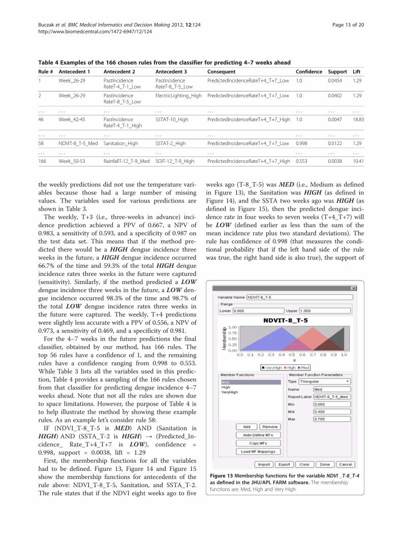
Table 4 Examples of the 166 chosen rules from the classifier for predicting 4–7 weeks ahead

Rule # Antecedent 1 Antecedent 2 Antecedent 3 Consequent Confidence Support Lift

1 Week_26-29 PastIncidenceRateT-4_T-1_Low

PastIncidenceRateT-8_T-5_Low

PredictedIncidenceRateT+4_T+7_Low 1.0 0.0454 1.29

2 Week_26-29 PastIncidenceRateT-8_T-5_Low

ElectricLighting_High PredictedIncidenceRateT+4_T+7_Low 1.0 0.0402 1.29

. . . . . . . . . . . . . . . . . . . . . . . .

46 Week_42-45 PastIncidenceRateT-4_T-1_High

SSTAT-10_High PredictedIncidenceRateT+4_T+7_High 1.0 0.0047 18.83

. . . . . . . . . . . . . . . . . . . . . . . .

58 NDVIT-8_T-5_Med Sanitation_High SSTAT-2_High PredictedIncidenceRateT+4_T+7_Low 0.998 0.0122 1.29

. . . . . . . . . . . . . . . . . . . . . . . .

166 Week_50-53 RainfallT-12_T-9_Med SOIT-12_T-9_High PredictedIncidenceRateT+4_T+7_High 0.553 0.0038 10.41

Figure 13 Membership functions for the variable NDVI _T-8_T-4as defined in the JHU/APL FARM software. The membershipfunctions are: Med, High and Very High.


the weekly predictions did not use the temperature vari-ables because those had a large number of missingvalues. The variables used for various predictions areshown in Table 3.The weekly, T+3 (i.e., three-weeks in advance) inci-

dence prediction achieved a PPV of 0.667, a NPV of0.983, a sensitivity of 0.593, and a specificity of 0.987 onthe test data set. This means that if the method pre-dicted there would be a HIGH dengue incidence threeweeks in the future, a HIGH dengue incidence occurred66.7% of the time and 59.3% of the total HIGH dengueincidence rates three weeks in the future were captured(sensitivity). Similarly, if the method predicted a LOWdengue incidence three weeks in the future, a LOW den-gue incidence occurred 98.3% of the time and 98.7% ofthe total LOW dengue incidence rates three weeks inthe future were captured. The weekly, T+4 predictionswere slightly less accurate with a PPV of 0.556, a NPV of0.973, a sensitivity of 0.469, and a specificity of 0.981.For the 4–7 weeks in the future predictions the final

classifier, obtained by our method, has 166 rules. Thetop 56 rules have a confidence of 1, and the remainingrules have a confidence ranging from 0.998 to 0.553.While Table 3 lists all the variables used in this predic-tion, Table 4 provides a sampling of the 166 rules chosenfrom that classifier for predicting dengue incidence 4–7weeks ahead. Note that not all the rules are shown dueto space limitations. However, the purpose of Table 4 isto help illustrate the method by showing these examplerules. As an example let’s consider rule 58:IF (NDVI_T-8_T-5 is MED) AND (Sanitation is

HIGH) AND (SSTA_T-2 is HIGH) → (Predicted_In-cidence_ Rate_T+4_T+7 is LOW), confidence =0.998, support = 0.0038, lift = 1.29First, the membership functions for all the variables

had to be defined. Figure 13, Figure 14 and Figure 15show the membership functions for antecedents of therule above: NDVI_T-8_T-5, Sanitation, and SSTA_T-2.The rule states that if the NDVI eight weeks ago to five

weeks ago (T-8_T-5) was MED (i.e., Medium as definedin Figure 13), the Sanitation was HIGH (as defined inFigure 14), and the SSTA two weeks ago was HIGH (asdefined in Figure 15), then the predicted dengue inci-dence rate in four weeks to seven weeks (T+4_T+7) willbe LOW (defined earlier as less than the sum of themean incidence rate plus two standard deviations). Therule has confidence of 0.998 (that measures the condi-tional probability that if the left hand side of the rulewas true, the right hand side is also true), the support of

Figure 15 Membership functions for the variable SSTA_T-2 asdefined in the JHU/APL FARM software. The membershipfunctions are: Low, Med and High.

Figure 14 Membership functions for the variable Sanitation asdefined in the JHU/APL FARM software. The membershipfunctions are: Low, Med and High.


0.0038 (so it describes 0.38% of the training data) and alift of 1.29.Our overall results on the test data for the 4–7 weeks

in the future prediction achieved a PPV of 0.686, a NPVof 0.976, a sensitivity of 0.615, and a specificity of 0.982and can be seen on Figure 16. The predictions on thetraining data are shown on Figure 17. For training data aPPV of 0.842, a NPV of 0.996, a sensitivity of 0.928, anda specificity of 0.99 were obtained. As mentioned previ-ously, good accuracy on the training data is relativelyeasy to achieve since the system has used that data forbuilding the model. The predictions on the validationdata are shown on Figure 18. For training data, a PPV of0.606, a NPV of 0.976, a sensitivity of 0.571, and a speci-ficity of 0.979 were obtained.Figure 19, Figure 20 and Figure 21 show the prediction

results for one district only: Iquitos - the district that hadthe most weeks with HIGH incidence rate from all thesix districts under consideration. The results on the testset are: a PPV of 1, which means that every time a HIGHvalue was predicted, an outbreak happened; a NPV of0.902; a sensitivity of 0.591; and a specificity of 1.

Logistic regression resultsIn order to compare the results of the novel technique pro-posed with those of an established method, we compared

FARM results with those of a method often used by epide-miologists: logistic regression (LR). We used the same in-put data for the LR models as for the FARM methods(see Table 3), for both weekly and four-week intervalpredictions.LR is a model used for prediction of the probability of

occurrence of an event and it is the method of choiceamong statisticians when the outcome (Y – the de-pendent variable) is binary. The goal of LR is to predictthe likelihood that Y is equal to 1 given certain values ofthe independent variables X1 through Xk. The form ofthe logistic model formula is:

p ¼ 1= 1þ exp � B0 þ B1�X1 þ B2

�X2 þ . . .þ Bk�Xkð Þð Þð Þ

where p is the probability that Y is 1, B0 is a constant(called the intercept), and B1 though Bk are the coeffi-cients for the predictor variables X1 through Xk.In our application, the LR result gives the probability

that a HIGH incidence rate will occur. Specifically, if theestimate exceeds a predefined threshold (0.5 in ourwork), the model predicts a HIGH incidence rate; other-wise, a HIGH is not predicted.For three-weeks in advance (T+3), LR yielded a PPV

of 0.5, a NPV of 0.962, a sensitivity of 0.25, and a specifi-city of 0.987. When predicting four-weeks in advance

Figure 16 4-Week prediction results for the test set.


(T+4), LR obtained PPV of 0.583, a NPV of 0.961, a sen-sitivity of 0.219, and a specificity of 0.992. The T+4through T+7 four week prediction using LR achieved aPPV of 0.178, a NPV of 0.949, a sensitivity of 0.205, anda specificity of 0.939. The coefficients obtained for thebest of LR models, four-weeks in advance (T+4) predic-tion, are shown in Table 5.The comparison of LR and FARM-based results is

shown in Figure 22, Figure 23 and Figure 24. FARM-based predictions provide much higher sensitivity thanLR’s. In 66% of cases FARM provides also much higherPPV than LR.

Figure 17 4-Week prediction results for the training set. When the bluerror. When the blue curve falls outside of the yellow bar, there is a predic

DiscussionA truly rigorous predictive method should have twocharacteristics that cannot be violated. The first one isthat the method cannot be both developed and tested onexactly the same data. Rigorous validation requires thatthe data used for testing not be the same as the dataused in its development. If the prediction method wasdeveloped and tested on the same data, then a highvalue of a performance metric, such as R2, does not re-veal anything about the accuracy that would occur onpreviously unseen data. Even obtaining R2=1 when usingthe same data for both development and validation does

e curve (actual) falls within the yellow bar (prediction) there is notion error.

Figure 18 4-Week prediction results for the validation set.


not guarantee a good prediction performance on datanot used for the model development.The second characteristic for rigorous prediction is

that all predictor variables need to be collected for theprevious time period (e.g. week) and be used for predic-tion of outbreaks during a later time period. Thisensures a realistic prediction because the values of allthe predictor variables can be obtained prior to perform-ing prediction for the next time period. Methods thatuse some variables at time T to predict another variableat time T (i.e., zero time lag) are not performing a usefulprediction because prediction means using past or cur-rently available data to describe a future event.When designing a prediction method that learns from

data, machine learning scientists very carefully divide

Figure 19 Prediction on the training data for Iquitos. The predicted Lovalues are shown in blue. The gaps with no values correspond to data thatthe green bar (predicted Low) or red bar (predicted High) there is no errorprediction error.

the data set they are using. Simply dividing the data setinto training (to develop the model) and testing (to testthe model and report performance) is considered insuffi-cient. These data should be divided into three subsets:training, validation and testing [46]. The training subsetis used to develop the model. The models are usuallynot parameter-free, but have certain parameters that canbe adjusted by the model developers: the best model isthe one that has the lowest error on the validation datasubset. Once the best model is chosen, then it becomesthe final version and it can be tested to assess its per-formance on a previously unseen data set called the test-ing subset. For example, in a feed-forward neuralnetwork, the number of hidden layers and the numberof neurons in each hidden layer are parameters to be

w is shown in green, the predicted High in red, and the actualwas not used in training. When the blue curve (actual) falls within. When the blue curve falls outside of those bars, there is a

Figure 20 Prediction on the validation data for Iquitos. The predicted Low is shown in green, the predicted High in red, and the actualvalues are shown in blue. The gaps with no values correspond to data that was not used in validation.


chosen; when several of those networks are compared,the best network has the smallest error on the validationdata subset. Once the network with the smallest valid-ation error is chosen, the error is computed for the testsubset in order to assess its performance on previouslyunseen data.It is important to note that our method only uses in-

put data that is actually available prior to running themodel at a given time. For example, for the Temperaturevariable, we ignored data within two weeks of thecurrent week in order to avoid using values that actuallywould not be available at the point in time at which theprediction is made. Temperature is provided in 8-dayintervals so, if such an interval ends on a Sunday, none

Figure 21 Prediction on Test data for Iquitos. The predicted Low is shoshown in blue. The gaps with no values correspond to data that was not u

of the Temperature values for the preceding week wouldbe available because the interval from which some oftheir data were coming would not be available until thefollowing Monday.Disease outbreak detection differs from prediction in

that the evidence of the incipient outbreak is alreadypresent though not yet obvious when it is first detected,and a response should begin immediately. Although itmay complement disease detection, the work presentedhere differs in that it can be used when no outbreak iscurrently present, and it predicts whether or not an out-break may occur at some specific time in the future. Re-sponse to such a prediction may include planning aswell as mitigation activities. Our method is designed to

wn in green, the predicted High in red, and the actual values aresed in testing.

Table 5 LR coefficients obtained for weekly predictions 4weeks ahead (T+4)

Variable LR Coefficient

Intercept 17.37

Week −0.01

PastIncidenceRate T-1 −2.30




PastIncidenceRate T-5 0.30








Rainfall T-1 0.01

Rainfall T-2 0.01

Rainfall T-3 0.00

Rainfall T-4 0.00

Rainfall T-5 0.00

Rainfall T-6 −0.01


Rainfall T-8 0.00

Rainfall T-9 0.00

Rainfall T-10 0.00

Rainfall T-11 0.00


NDVI T-4 0.20

NDVI T-5 3.83

NDVI T-6 −5.59

NDVI T-7 1.86

NDVI T-8 −3.45

NDVI T-9 1.84

NDVI T-10 −5.75

NDVI T-11 −1.99

NDVI T-12 −5.21

SSTA T-1 −2.11

SSTA T-2 1.21

SSTA T-3 −0.79

SSTA T-4 1.16

Figure 22 Comparison of LR and FARM-based results forweekly predictions three-weeks in advance (T+3).

Figure 23 Comparison of LR and FARM-based results forweekly predictions four-weeks in advance (T+4).


produce a dengue outbreak prediction four to sevenweeks in advance, thereby providing public health offi-cials with more time to intervene and perhaps mitigatethe impacts of an outbreak. Discussions with ourPeruvian collaborators revealed that this response time-line is reasonable for their public health departments.They did caution however, that it is important to have a

method with few false alarms because of limited fundingfor public health interventions. The parameter of great-est importance to these public health practitioners istherefore PPV, with specificity being second in priority.Our method has several weaknesses. First, it has no in-

put variables that directly measure vector behavior, e.g.,mosquito biting behavior or prevalence of dengue virusin the vector. This information is quite important, yet isexpensive and labor intensive to obtain, and possibleonly for small areas over short time periods. The reasonwe are not using this variable is that we do not have ac-cess to such data for Peru. Also, because the socio-political and sanitation data are only available as annualupdates, our method cannot predict the effects of con-centrated sanitation programs such as house-to-houseefforts to remove vector breeding containers. Anothervariable that could be useful for prediction are people’stravel patterns. If people were traveling from a districtwith an ongoing outbreak, these data have the potentialto be important predictors. Additionally, we do not have

Figure 24 Comparison of LR and FARM-based results for fourweek interval prediction: weeks T+4 through T+7.


historical data describing the serotypes present andexisting dogma supports a role for pre-existing immun-ity to a serotype with which a person was infected be-fore. Given the fact that the methodology developedherein automatically extracts rules from existing data,the weaknesses described above can be overcome shouldthe data become available.

ConclusionsThe method described above was developed to use localand remote sensing data to predict dengue outbreaks,with an outbreak defined as being above the long-termmean previous dengue incidence plus two standarddeviations, with high values of PPV and NPV. Effectivemethodologies to predict disease outbreaks may allowpreventive interventions to avert large epidemics. Forbest results, the researchers must have access to datastreams with timely, detailed, and accurate values of pre-dictor variables. Model validation is of paramount im-portance as health officials would be unlikely to spendresources on mitigation efforts based on model predic-tions without evidence of accuracy on past outbreaks.The input variables used in our model are widely avail-able for most, if not all, countries. Although additionallocal data, such as mosquito biting activity or percentageof mosquitoes with dengue virus, might improve the ac-curacy of our method, such data are generally difficultand expensive to obtain. The use of widely available dataenhances the generalizability of our method.

Competing interestsThe authors’ declare that they have no competing interests.

Authors’ contributionsALB directed the project, conceived the prediction methodology used, runthe fuzzy association rule mining and classification software to obtainprediction results. She wrote portions of the manuscript and contributed toreviewing of the manuscript. PTK conceived the methods for preprocessingthe data to fit the spatiotemporal scale, and implemented all routines in

MATLAB to do the preprocessing. He also developed the Logistic RegressionModel. He wrote a part of the rough draft of the manuscript. SMBcontributed satellite remote sensing (e.g., selection of satellite products) andatmospheric science expertise, as well as medical expertise to the analysisand interpretation of the data. He contributed to the writing of themanuscript. BHF contributed his medical and public health expertise to theinterpretation of the data. He wrote portions of the manuscript. SHL wasinstrumental in acquiring the epidemiological data. She contributed to thewriting and reviewing of the manuscript. All authors read and approved thefinal manuscript.

DisclaimerThe views expressed here are the opinions of the authors and are not to beconstrued as official or as representing the views of the US Department ofthe Navy or the US Department of Defense.

AcknowledgementsWe gratefully acknowledge the support of the Ministerio de Salud del Peru,especially Dr. Omar Napanga, for the dengue case surveillance data andmany helpful discussions. We also are in debt to Dr. Carlos Sanchez and Dr.Joel Montgomery of the US Naval Medical Research Center, Lima, Peru, andCAPT Clair Witt of the US Armed Forces Health Surveillance Center. Fundingfor this study was provided by the US Department of Defense GlobalEmerging Infections Surveillance and Response System, a division of the USArmed Forces Health Surveillance Center.

Received: 1 May 2012 Accepted: 25 October 2012Published: 5 November 2012

References1. Focks DA, Daniels E, Haile DG, Keesling JE: A simulation model of the

epidemiology of urban dengue fever: literature analysis, modeldevelopment, preliminary validation, and samples of simulation results.Am J Trop Med Hyg 1995, 53(5):489–506.

2. Gibbons RV, Vaughn DW: Dengue: an escalating problem. BMJ 2002,324(7353):1563–1566.

3. TDR/WHO: Dengue Guidelines for Diagnosis, Treatment, Prevention andControl. Geneva: World Health Organization; 2009. Available:http://whqlibdoc.who.int/publications/2009/9789241547871_eng.pdf.Accessed 26 October 2012.

4. Ranjit S, Kissoon N: Dengue hemorrhagic fever and shock syndromes.Pediatr Crit Care Med 2010, 12(1):90–100.

5. Guzman MG, Kouri G: Dengue: an update. Lancet Infect Dis 2002, 2:33–42.6. Halsted SB: Dengue. Lancet Infect Dis 2007, 370:1644–1652.7. US Centers for Disease Control and Prevention: Locally Acquired

Dengue – Key West, Florida 2009–2010. MMWR 2010, 59(19):577–581.8. Heymann DL (Ed): Control of Communicable Diseases Manual. 19th edition.

Washington DC: American Public Health Association; 2008.9. Tan GK, Alonso S: Pathogenesis and prevention of dengue virus infection:

state of the art. Curr Opin Infect Dis 2009, 22(3):302–308.10. Fuller DO, Troyo A, Beier JC: El Nino Southern Oscillation and vegetation

dynamics as predictors of dengue fever cases in Costa Rica. Environ ResLett 2009, 4:014011.

11. Choudhury MAHZ, Banu S, Islam MA: Forecasting dengue incidence inDhaka, Bangladesh: a time series analysis. DF Bulletin 2008, 32:29–37.

12. Wongkoon S, Jaroensutasinee M, Jaroensutasinee K: Predicting DHFincidence in northern Thailand using time series analysis technique.World Academy of Science, Engineering and Technology 2007, 32:216–220.

13. Cummings DAT, Irizarry RA, Huang NE, Endy TP, Nisalak A, Ungchusak K,Burke DS: Travelling waves in the occurrence of dengue haemorrhagicfever in Thailand. Nature 2004, 427:344–347.

14. Bhandari KP, Raju PLN, Sokhi BS: Application of GIS modeling for denguefever prone area based on socio-cultural and environmental factors – acase study of Delhi city zone. The International Archives of thePhotogrammetry, Remote Sensing and Spatial Information Sciences, Vol.XXXVII, Part B8 2008, 165–170. Beijing, China.

15. Husin NA, Salim N, Ahmad AR: Modeling of dengue outbreak predictionin Malaysia: a comparison of neural network and nonlinear regressionmodel. IEEE International Symposium on Information Technology (ITSim 2008)2008, 3:1–4. Kuala Lumpur, Malaysia.

http://whqlibdoc.who.int/publications/2009/9789241547871_eng.pdf


16. Cetiner BG, Sari M, Aburas HM: Recognition of dengue disease patternsusing artificial neural networks. In 5th International Advanced TechnologiesSymposium (IATS’09). Karabuk: 2009:359–362.

17. Rachata N, Charoenkwan P, Yooyativong T, Camnongthai K, Lursinsap C,Higachi K: Automatic prediction system of dengue haemorrhagic-feveroutbreak risk by using entropy and artificial neural network. IEEEInternational Symposium on Communications and Information Technologies(ISCIT 2008) 2008, 210–214. 21–23 October 2008, Lao.

18. Fu X, Liew C, Soh H, Lee G, Hung T, Ng L-C: Time-series infectious diseasedata analysis using SVM and genetic algorithm. 2007 IEEE Congress onEvolutionary Computation (CEC 2007) 2007, 1276–1280. Singapore, 25–28September 2007.

19. Halide H, Ridd P: A predictive model for dengue hemorrhagic feverepidemics. International J Environ Health Research 2008, 4:253–265.

20. Honório NA, Nogueira RMR, Codeco CT, Carvalho MS, Cruz OG, MagalhaesMAFM, de Araujo JMG, de Araujo ESM, Gomes MQ, Pinheiro LS, Pinel CS, deOliveira L: Spatial evaluation and modeling of dengue seroprevalenceand vector density in Rio de Janeiro, Brazil. PLoS Negl Trop Dis 2009,3:e545.

21. Barbazan P, Guiserix M, Boonyuan W, Tuntaprasart W, Pontier D,Gonzalez J-P: Modelling the effect of temperature on transmission ofdengue. Medical and Veterinary Entomology 2010, 24:66–73.

22. Kummerow C, Barnes W, Kozu T, Shiue J, Simpson J: The Tropical RainfallMeasuring Mission (TRMM) sensor package. J. Atmos. Ocean. Technol.1998, 15:809–817.

23. Soebiyanto RP, Adimi F, Kiang RK: Modeling and predicting seasonalinfluenza transmission in warm regions using climatological parameters.PLoS One 2010, 5:e9450.

24. Anyamba A, Linthicum KJ, Mahoney R, Tucker CJ, Kelley PW: Mappingpotential risk of Rift Valley Fever outbreaks in African savannas usingvegetation index time series data. Photogramm. Engr. Remote Sens. 2002,68:137–145.

25. Hales S, Weinstein P, Souares Y, Woodward A: El Nino and the dynamics ofvectorborne disease transmission. Environ Health Perspect 1999,107:99–102.

26. Johansson MA, Cummings DAT, Glass GE: Multiyear climate variability anddengue – El Nino Southern Oscillation, weather, and dengue incidencein Puerto Rico, Mexico, and Thailand: a longitudinal data analysis.PLoS Med 2009, 6:e1000168.

27. Hu W, Clements A, Williams G, Tong S: Dengue fever andEl Nino/Southern Oscillation in Queensland, Australia: a time seriespredictive model. Occup Environ Med 2010, 67:307–311.

28. US Centers for Disease Control and Prevention: MMWR Weeks. 2012.Available: http://www.cdc.gov/nndss/document/MMWR_Week_overview.pdfAccessed 26 October 2012.

29. US National Aeronautics and Space Administration Goddard Earth SciencesData and Information Services Center: Mirador Earth Science Data SearchTool. 2012. Available: http://mirador.gsfc.nasa.gov/ Accessed 26 October2012.

30. Mathworks: MATLAB. Available: http://www.mathworks.com/products/matlab/index.html Accessed 26 October 2012.

31. US Geological Survey: Land Processes Distributed Active Archive Center.Available: https://lpdaac.usgs.gov/get_data Accessed 26 October 2012.

32. Kalluri S, Gilruth P, Rogers D, Szczur M: Surveillance of arthropodvector-borne infectious diseases using remote sensing techniques: areview. PLoS Pathog 2007, 3(10):e116. doi:10.1371/journal.ppat.0030116.

33. Ferreira NC, Ferreira LG, Huete AR: Assessing the response of the MODISvegetation indices to landscape disturbance in the forested areas of thelegal Brazilian Amazon. International J Remote Sensing, 31(3):745–759.

34. Xiao X, Zhang Q, Saleska S, Hutyra L, De Camargo P, Wofsy S, Frolking S,Boles S, Keller M, Moore B: Satellite-based modeling of gross primaryproduction in a seasonally moist tropical evergreen forest. RemoteSensing Environ 2005, 94:105–122.

35. Climate and Global Dynamics Section, US National Center for AtmosphericResearch, University Corporation for Atmospheric Research: SouthernOscillation Index Data. Available: http://www.cgd.ucar.edu/cas/catalog/climind/SOI.signal.ascii Accessed 26 October 2012.

36. Global Change Master Directory, US National Aeronautics and SpaceAdministration Goddard Space Flight Center: Monthly and Weekly Nino 3.4Region SST Index: East Central Tropical Pacific. 2012. Available: http://gcmd.

nasa.gov/records/GCMD_NOAA_NWS_CPC_NINO34.html Accessed 26October 2012.

37. The World Bank Group: Worldwide Governance Indicators. 2012. Available:http://info.worldbank.org/governance/wgi/index.asp Accessed 26 October2012.

38. Peru National Institute of Statistics and Information. Peru: Census; 2007.Available: http://www.inei.gob.pe/ Accessed 26 October 2012.

39. US National Oceanic and Atmospheric Administration, National GeophysicalData Center: Topographic and Digital Terrain Data. Availablehttp://www.ngdc.noaa.gov/cgi-bin/mgg/ff/nph-newform.pl/mgg/topo/Accessed 26 October 2012.

40. Buczak AL, Gifford CM: Fuzzy association rule mining for communitycrime pattern discovery. In Proceedings of the ACM SIGKDD Conference onKnowledge Discovery and Data Mining: Workshop on Intelligence and SecurityInformatics. Washington, D.C: Association for Computing Machinery; 2010.July 2010.ISBN 978-1-4503-0223-4/10/07.

41. Kuok CM, Fu A, Wong MH: Mining fuzzy association rules in databases.ACM SIGMOD Record 1998, 27(1):41–46. New York, NY.

42. Zadeh LA: Fuzzy Sets. Information and Control 1965, 8(3):338–353.43. Liu B, Hsu W, Ma Y: Integrating classification and association rule mining.

In Proceedings of 4th International Conference on Knowledge Discovery DataMining (KDD). New York: AAAI Press; 1998:80–86.ISBN 1-57735-070-7.

44. Agrawal R, Imielinski T, Swami A: Mining association rules between sets ofitems in large databases. In Proceedings of the International Conference onManagement of Data. Washington, DC: Association for ComputingMachinery; 1993:207–216.

45. Srikant R, Agrawal R: Mining quantitative association rules in largerelational tables. In Proceedings of the International Conference onManagement of Data. Montreal: Association for Computing Machinery;1996:1–12.

46. Cawley GC, Talbot NLC: On over-fitting in model selection andsubsequent selection bias in performance evaluation. J Machine LearningRes 2010, 11:2079–2107.

doi:10.1186/1472-6947-12-124Cite this article as: Buczak et al.: A data-driven epidemiologicalprediction method for dengue outbreaks using local and remotesensing data. BMC Medical Informatics and Decision Making 2012 12:124.

Submit your next manuscript to BioMed Centraland take full advantage of:

• Convenient online submission

• Thorough peer review

• No space constraints or color figure charges

• Immediate publication on acceptance

• Inclusion in PubMed, CAS, Scopus and Google Scholar

• Research which is freely available for redistribution

Submit your manuscript at www.biomedcentral.com/submit

http://www.cdc.gov/nndss/document/MMWR_Week_overview.pdf

http://mirador.gsfc.nasa.gov/

http://www.mathworks.com/products/matlab/index.html

http://www.mathworks.com/products/matlab/index.html


http://dx.doi.org/10.1371/journal.ppat.0030116

http://www.cgd.ucar.edu/cas/catalog/climind/SOI.signal.ascii

http://www.cgd.ucar.edu/cas/catalog/climind/SOI.signal.ascii

http://gcmd.nasa.gov/records/GCMD_NOAA_NWS_CPC_NINO34.html

http://gcmd.nasa.gov/records/GCMD_NOAA_NWS_CPC_NINO34.html

http://info.worldbank.org/governance/wgi/index.asp

http://www.inei.gob.pe/

http://www.ngdc.noaa.gov/cgi-bin/mgg/ff/nph-newform.pl/mgg/topo/

a data-driven epidemiological prediction method for dengue ... · a data-driven epidemiological...

Documents