A database of polarised K3 surfaces

Gavin Brown∗

Abstract

We describe a computer-based database of polarised K3 surfacesand explain the meaning of the information it contains. In a precisesense, the database includes all K3 surfaces.

Contents

1 Introduction 2

2 Families of K3 surfaces 42.1 Polarised K3 surfaces . . . . . . . . . . . . . . . . . . . . . . . 52.2 The meaning of the K3 database . . . . . . . . . . . . . . . . 82.3 Elliptic fibrations and Shimada’s classification . . . . . . . . . 10

3 Numerical unprojection and weights 143.1 Type I and Type IIn unprojections . . . . . . . . . . . . . . . 143.2 K3 surfaces admitting no Gorenstein projection . . . . . . . . 18

4 Using the K3 database 19

A Tables of results 22

∗gdb@kent.ac.uk Address: IMSAS, University of Kent, Canterbury, CT2 7NF, UK.This paper was written at the University of Warwick under EPSRC grant GR/S03980/01Algebraic geometry, graded rings and computer algebra.

1

1 Introduction

Many authors have compiled lists of K3 surfaces embedded in weighted pro-jective space (wps). The first of these lists is the ‘famous 95’ weighted hyper-surfaces of Reid [1980] (Theorem 4.5) and others. Next there are 84 familiesof K3 surfaces in codimension 2 computed by Fletcher [2000] (section 13.8),followed by 70 families in codimension 3 and 142 families in codimension 4both computed by Altınok [1998]. Such lists could be continued indefinitelyin increasing codimension, as there are countably many deformation fami-lies of polarised K3 surfaces, although the construction of explicit equationsbecomes difficult.

We extend the classification of polarised K3 surfaces to give a list thatcontains the numerical data of all polarised K3 surfaces in the precise senseof Theorem 8 below. Although the list of families of polarised K3 surfaces isinfinite, the numerical data we work with behave in a regular way after thefirst 15,000 or so families are obtained, and so a finite list can summarise thewhole classification. Even so, it is far too large to be reproduced in the waythat the existing lists have been. In fact, both the analysis used to createthe list and methods of interrogating it are handled by a computer. Theresulting list of 24,099 numerical K3 candidates (see Definition 6) is known asthe K3 database. It was created using the computer algebra system Magma

[Cannon, 2005; Bosma et al., 1997], and it is accessible in three ways: one canrun Magma itself, or connect to the web interface at [Brown et al., 2004]

(which runs Magma in the background) or install a SQL-style database[Brown and Kerber, 2005] prepared from the on-line version. These arediscussed in section 4. Although computer access is the only serious way toaddress such a database, K3 surfaces in low codimension are also available at[Brown et al., 2004] including a new list of 163 K3 surfaces in codimension 5.

The main results of this paper explain the meaning of the K3 database.We make this explicit in Meanings 7, 9, 10, 18. Theorem 8 explains thesense in which it is comprehensive and the way in which we regard the K3database as an upper bound for the numerical data of polarised K3 surfaces.An immediate corollary is a sharp lower bound on the degree of polarised K3surfaces; see section 4 for Magma code that makes this calculation.

Computation 1 If X, A is a polarised K3 surface, then the degree A2 of Xis at least 1/330. In more detail, both the degree A2 and the Picard numberρX ≤ 20 of X are bounded below according to the genus g = h0(X, A) − 1 as

2

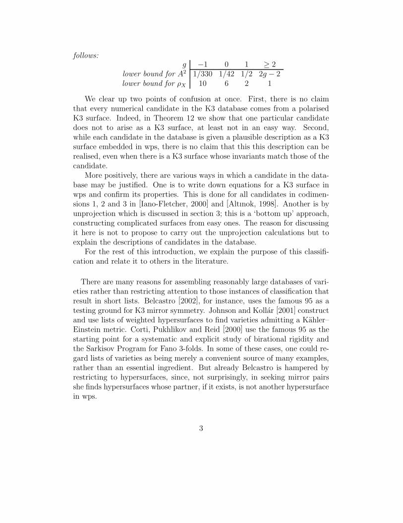
follows:g −1 0 1 ≥ 2

lower bound for A2 1/330 1/42 1/2 2g − 2lower bound for ρX 10 6 2 1

We clear up two points of confusion at once. First, there is no claimthat every numerical candidate in the K3 database comes from a polarisedK3 surface. Indeed, in Theorem 12 we show that one particular candidatedoes not to arise as a K3 surface, at least not in an easy way. Second,while each candidate in the database is given a plausible description as a K3surface embedded in wps, there is no claim that this this description can berealised, even when there is a K3 surface whose invariants match those of thecandidate.

More positively, there are various ways in which a candidate in the data-base may be justified. One is to write down equations for a K3 surface inwps and confirm its properties. This is done for all candidates in codimen-sions 1, 2 and 3 in [Iano-Fletcher, 2000] and [Altınok, 1998]. Another is byunprojection which is discussed in section 3; this is a ‘bottom up’ approach,constructing complicated surfaces from easy ones. The reason for discussingit here is not to propose to carry out the unprojection calculations but toexplain the descriptions of candidates in the database.

For the rest of this introduction, we explain the purpose of this classifi-cation and relate it to others in the literature.

There are many reasons for assembling reasonably large databases of vari-eties rather than restricting attention to those instances of classification thatresult in short lists. Belcastro [2002], for instance, uses the famous 95 as atesting ground for K3 mirror symmetry. Johnson and Kollar [2001] constructand use lists of weighted hypersurfaces to find varieties admitting a Kahler–Einstein metric. Corti, Pukhlikov and Reid [2000] use the famous 95 as thestarting point for a systematic and explicit study of birational rigidity andthe Sarkisov Program for Fano 3-folds. In some of these cases, one could re-gard lists of varieties as being merely a convenient source of many examples,rather than an essential ingredient. But already Belcastro is hampered byrestricting to hypersurfaces, since, not surprisingly, in seeking mirror pairsshe finds hypersurfaces whose partner, if it exists, is not another hypersurfacein wps.

3

The main reason for extending the lists as we do is as part of the classi-fication of Fano 3-folds. We explain this briefly; see [Altınok et al., 2002] formuch greater detail. A 3-fold X is a Fano 3-fold if it has at worst Q-factorialterminal singularities and −KX is ample—it is common to insist that more-over Pic(X) = Z and −KX is a generator. By [Kawamata, 1992], there areonly finitely many deformation families of Fano 3-folds. If the linear system| − KX | contains an irreducible surface S with only Du Val singularities,then S is a K3 surface and it is polarised by the trace of −KX . Such asurface S is called a K3 elephant for X, and the vast majority of known Fano3-folds have a K3 elephant. The main point of [Altınok et al., 2002] is toattempt the converse operation: given a polarised K3 surface S, A, constructa Fano 3-fold X having S as its K3 elephant. This can be regarded as adeformation–extension problem, in which one must include a new variable inthe equations of S while maintaining the irreducibility (at the very least) ofthe locus they define. From this point of view, the K3 database contains acoarse classification of Fano-with-elephant 3-folds as a finite sublist (althoughexactly which sublist is the interesting point).

There are many other lists of varieties we could mention. Following clas-sifications by Miranda and Persson [1989] and others, Shimada and Zhang[2001], [Shimada, 2000] classify K3 surfaces that arise as elliptic fibrations.Kreuzer and Skarke [1998] classify K3 surfaces that arise as toric hyper-surfaces, and in higher dimension, they classify Calabi–Yau 3-fold toric hy-persurfaces [Kreuzer and Skarke, 2000]. Their famous Calabi–Yau databasecontains nearly 500 million families of Calabi–Yau 3-folds; it is not knownwhether there are infinitely many families or not. Buckley and Szendroi[2005], [Buckley, 2003] construct Calabi–Yau 3-folds by methods similar tothose we use here, although their interest is not in constructing lists of vari-eties but rather to find examples not already in the vast Kreuzer–Skarke list.More recently, Caravantes [2005] computes examples of Fano 3-folds that arequotients of other Fano 3-folds—so-called Fano–Enriques 3-folds—in codi-mension at most 3, and Kasprzyk [2003; 2005] computes the classificationsof toric Fano 3-folds under various hypotheses.

2 Families of K3 surfaces

The methods used here follow Altınok’s approach using Hilbert series, asexplained in Altınok–Brown–Reid [2002].

4

2.1 Polarised K3 surfaces

A polarised K3 surface is a pair X, A where X is a surface having only Du Valsingularities, trivial canonical divisor KX = 0 and irregularity q = 0, whileA is an ample divisor on X. Recall that a Du Val singularity (or Kleinianor ADE singularity) is the germ at the origin of C2/G where G ⊂ SL(2, C)is a finite group; equivalent conditions, see [Durfee, 1979] or [Reid, 1980],include being defined by an equation from the list of ADE normal forms, orimposing no conditions on adjuction so that the canonical class pulls backto a minimal resolution. Throughout this paper, K3 surface refers to such apair X, A.

Graded ring of a K3 surface A polarised K3 surface has a graded ringR(X, A) = ⊕n≥0H

0(X, nA), and the Hilbert series PX(t) of X, A is definedto be the Hilbert series of this graded ring:

PX(t) =∑

t≥0

h0(X, nA)tn.

Since A is ample, R(X, A) is a finitely-generated k-algebra and the Projcorrespondence embeds X in wps:

X = Proj R(X, A) ⊂ PN for some PN = P(a0, . . . , aN)

where we suppose that R(X, A) is minimally generated as a k-algebra by ho-mogeneous elements x0, . . . , xN ∈ R(X, A) with deg xi = ai. A minimal freeresolution of R(X, A) as a k[PN ]-module then exhibits a preferred rationalform of the formal power series PX(t):

PX(t) =HX(t)∏(1 − tai)

(1)

where HX(t) is a polynomial, the Hilbert numerator of X, A and the de-nominator product is taken over the weights a0, . . . , aN of the wps PN . Thecodimension of X, A is defined to be the codimension of X in this embedding.The genus of X, A is h0(X, A) − 1, which is an integer ≥ −1.

Riemann–Roch and baskets of singularities Altınok’s Riemann–Rochformula, Theorem 2 below, computes the Hilbert series of a K3 surface X, A.It involves the notion of a basket of quotient singularities, which is explainedbelow, to compute the effect of the singularities of X, A on h0(X, nA).

5

Theorem 2 (Altınok[1998] Theorem 4.6, [2003] 3.2) Let X, A be a po-larised K3 surface. Then

PX(t) =1 + t

1 − t+

t(1 + t)

(1 − t)3

A2

2−

∑

B

1

(1 − tr)

r−1∑

i=1

bi(r − bi)ti

2r(2)

where

A2 = 2g − 2 +∑

B

b(r − b)

r. (3)

In these formulas, B is a collection of cyclic quotient singularities 1

r(a,−a) at

which the polarising divisor A restricts to the eigensheaf La of the quotient.The notation x denotes the minimal nonnegative residue of x modulo r, andb = b satisfies ab = 1.

The collection B of cyclic quotient singularities is called the basket of singu-larities of X, A. It computes the contribution of the actual singularities ofX, A to Riemann–Roch. In general the singularities of X may differ from B.This phenomenon is well-known since [Reid, 1980] and [Reid, 1987], althoughhere we need to know how baskets arise.

If p ∈ X is a Du Val singularity, then it is also polarised by A—this globalpolarising divisor restricts to some element of the local class group of p ∈ X.Taking a small analytic neighbourhood p ∈ U ⊂ X, there is a deformationof U, A|U so that the general fibre Ut, At has only cyclic quotient singularitiesand at each such q ∈ Ut the divisor At restricts to a generator of the localclass group. Thus q ∈ Ut is of type 1

r(a,−a) for coprime 0 < a < r. Let Bp be

the collection of these polarised cyclic quotient singularities. This collectionBp is uniquely determined by the polarised singularity p ∈ X. Finally, B isthe collection of all Bp as p runs through the Du Val singularities of X. Thefollowing result is implicit in [Reid, 1987] (9.4).

Lemma 3 In the notation above, let Γp be the dual graph of the resolutionof p ∈ X and Γq1

, . . . , Γqkbe those of the basket Bp. Then the disjoint union

∪Γqiembeds as a subgraph of Γp so that no two components, Γqi

and Γqjfor

i 6= j, are joined by an edge of Γp.

6

Proof By [Reid, 1987] (9.4) and (4.10) (suitably re-ordered), the only po-larised Du Val singularities that lead to a non-empty basket are:

p ∈ X basketAnk−1 k × An−1

D2k−1 (2k + 1) × A1

Dk+2 2 × A1

E6 2 × A2

D2k k × A1

E7 3 × A1.

(4)

In each case, the dual graphs of the basket can be arranged as a disconnectedsubgraph of Γp as claimed. Q.E.D.

It would be convenient to know that X deforms to a K3 surface with singu-larities equal to the basket, but we do not know that or need it.

Proposition 4 If B is a basket for a K3 surface of genus g, then

∑

B

(r − 1) ≤ 19 and 2g − 2 +∑

B

b(r − b)

r> 0.

Furthermore, if the singularities of B lie on a surface Y , then the minimalresolution of these singularities must not contain 17 disjoint −2-curves andall coefficients of the power series P (t) computed by formula (2) are nonnegative.

Proof If the singularities of X are equal to those of the basket (as polarisedsingularities), then all the claims are standard: the first comes from thebound on the Picard rank of the resolution; the second is A2 > 0; the thirdis a standard consequence of the Torelli theorem. Even if the singularitiesof X are not those of B, the second inequality holds automatically since thebasket computes A2 exactly.

In general, Lemma 3 shows that the number of exceptional curves in aresolution of X is at least that in the resolution of its basket, and moreoverif one can find k disjoint −2-curves in the resolution of the basket then thesame is true for the resolution of singularities of X itself. Q.E.D.

7

Computation 5 Let Bg be the set of baskets which appear in Riemann–Rochfor a K3 surface with genus g ≥ −1. Then Bg is finite and of size

g −1 0 1 ≥ 2#Bg 4281 6479 6627 6628

and moreover Bg = B2 whenever g ≥ 3.

When g ≤ 2, this is the result of a simple computer enumeration of allpossible baskets of singularities of type 1

r(a,−a) for coprime 0 < a < r

satisfying the four conditions of Proposition 4. The fact that Bg = B2 wheng ≥ 3 is immediate from the form of the degree condition A2 > 0. The‘missing’ basket in genus 1 is the empty one: there is no nonsingular K3surface with g = 1.

2.2 The meaning of the K3 database

The K3 database is intended to represent all possible K3 surfaces X, A. Herewe say in what sense every K3 surface appears in the database, and converselywe begin to see to what extent items in the database come from K3 surfaces.

Definition 6 A numerical K3 candidate is a pair (g,B), where g ≥ −1 isan integer and B is a basket from the set Bg constructed in Computation 5.

A numerical K3 candidate contains exactly the data needed to compute aHilbert series using the formula of Theorem 2.

Meaning 7 The K3 database is a finite set DK3 whose elements are numer-ical K3 candidates. It includes the candidates (g,B) for −1 ≤ g ≤ 2 and allB ∈ Bg.

For each candidate ξ = (g,B), we define formally a degree denoted A2ξ

and a Hilbert series denoted Pξ(t) by the formulas (3) and (2) respectively.

Theorem 8 (Completeness of the K3 database) Let X, A be a polar-ised K3 surface of genus g. Then X, A is represented in the K3 database DK3

as follows:

• if g ≤ 2, then there is a numerical K3 candidate ξ = (g,B) ∈ DK3 with

A2 = A2

ξ and PX(t) = Pξ(t).

8

• if g ≥ 3, then there is a numerical K3 candidate ξ = (2,B) ∈ DK3 with

A2 = A2

ξ + 2(g − 2) and PX(t) = Pξ(t) +t(1 + t)

(1 − t)3(g − 2).

Proof If g ≤ 2, then this follows immediately from Theorem 2 and Propo-sition 4. When g ≥ 3, it holds because B2 = Bg from Computation 5 impliesthat the formulas (3) and (2) differ from the g = 2 case only by the 2g termin A2.

Q.E.D.

Weights and codimension The K3 database includes extra informationabout each entry: each ξ ∈ DK3 has a sequence of weights (a0, . . . , aN)associated to it with positive integers ai. The hope is that a K3 surfaceX, A exists with numerical data ξ and embedded by (all multiples of) A inPN(a0, . . . , aN).

The naive method to generate such weights generalises the first examplessuch as in [Altınok et al., 2002] section 1; variations of it are describedin [Iano-Fletcher, 2000] (section 18). If Pξ(t) = 1 + p1t + p2t

2 + · · · is theHilbert series of some ring R, then R must have p1 generators in degree 1. Wecompute (1−t)p1Pξ = 1+p′kt

k +· · · where p′k is the first nontrivial coefficient.If p′k > 0, then R must also have p′

k generators in degree k; in that case wecompute (1 − t)p1(1 − tk)p′

kPξ and continue. If p′k < 0, then R must have atleast |p′k| relations in degree k; in that case we stop the calculation and letthe weights of ξ be the collection of weights of all generators deduced so far.

Thus, just as in section 2.1, the weights determine a preferred rationalexpression for the corresponding Hilbert series. Its numerator is again calledthe Hilbert numerator and is denoted Hξ(t) in this context. (In principle,it is possible that the calculation breaks down too soon and Hξ is not apolynomial, but in practice this does not happen.) In this way, the weightsof ξ determine a prediction of a K3 surface X ⊂ PN(a0, . . . , aN) that realisesξ. With this in mind, the codimension of ξ is defined to be N − 2.

Meaning 9 The K3 database DK3 comprises all pairs (g,B) with g ≤ 2 andB ∈ Bg together with those pairs with 3 ≤ g ≤ 9 having codimension at most7. For each genus g, the pairs (g,B) are listed in increasing order of Hilbertseries.

9

The order on Hilbert series is of course the natural lexicographic order. Theweights, and hence the codimension, are those computed in section 3 usingmore systematic methods than the naive one above. The number of numericalK3 candidates per genus and codimension is listed in Table 1 of Appendix A.

Degenerations of graded rings Of course, the Hilbert series of a gradedring does not determine that ring. Whichever method is used to compute theweights, they are not expected to match every K3 surface X, A with givenHilbert series.

Meaning 10 If X, A is a K3 surface with genus ≤ 2, then the Hilbert seriesPX,A(t) of X will be that of some ξ ∈ DK3. However, the weights assignedto the candidate ξ will not necessarily be those of a set of generators of thegraded ring R(X, A).

Consider the well-known example of a general complete intersection ofequations of degrees 2 and 4

Y2,4 ⊂ P4(1, 1, 1, 1, 2)

where the weight 2 variable does not appear in the degree 2 equation. ThisK3 surface has the same Hilbert series as the quartic surface in P3. Thecorresponding ξ ∈ DK3 (which is listed even though g = 3) is assigned weights(1, 1, 1, 1), the weights of a typical example in P3, rather than the weights ofP4 above.

In [Brown, 2005], a computer search with Magma found other degener-ations of K3 surfaces in codimension 1 and 2. We reproduce some resultsof that search in Table 4 in Appendix A as an illustration, but see [Brown,2005] for more and for the combination of degeneration and unprojectioncalculations behind them.

2.3 Elliptic fibrations and Shimada’s classification

By Theorem 8, the K3 database contains all K3 surfaces (at least of genus≤ 2). From now on, we consider the converse: which candidates in thedatabase actually arise as K3 surfaces. We understand a two different positiveanswers.

10

Definition 11 Let ξ ∈ DK3 be a numerical K3 candidate from the K3 data-base and (a0, . . . , aN) its weights. We say that

(a) ξ represents a K3 Hilbert series if there is a polarised K3 surface X, Awith PX(t) = Pξ(t).

(b) ξ represents a K3 surface if there is a polarised K3 surface X, A withPX(t) = Pξ(t) whose graded ring R(X, A) has a generating set x0, . . . , xN ∈R(X, A) which are homogeneous of degrees deg xi = ai.

We consider the stronger statement (b) in section 3 below. The naturalapproach to (a) is to apply the Torelli theorem for K3 surfaces; we do not dothat here, although it is a straightforward computer calculation to confirmthat all candidates in codimension up to 6 do at least represent a K3 Hilbertseries. Instead, we compare our database with a classification of elliptic K3surfaces due to Shimada [2000].

An elliptic K3 surface is a fibration f : Y → P1 where Y is a nonsingularK3 surface and the general fibre is a curve of genus 1. (We do not assume thatf has a section.) Shimada [2000] classifies the collections of singular fibresthat do appear on elliptic K3 surfaces into 3937 different collections (manyof which can appear in fibrations having different numbers of sections).

A nonexistence result There are candidates that cannot easily representa K3 Hilbert series. A polarisation A is said to be simple if it intersectsthe exceptional locus of each singularity transversely at a single point. Thecandidate in the theorem below is number 76 (of genus 0) in DK3.

Theorem 12 Let ξ = (g,B) ∈ DK3 be the candidate with g = 0 and B ={1

2(1, 1), 2× 1

10(1, 9)}. Then there does not exist a polarised K3 surface X, A

with PX(t) = Pξ(t) for which the polarisation is simple.

Proof Suppose X, A is a polarised K3 surface with PX(t) = Pξ(t). We haveH0(X, A) = 1 since g = 0, so we may regard A ⊂ X as an effective divisorwith A2 = −2. Let ϕ : Y → X be the minimal resolution of singlarities; Y isa nonsingular K3 surface. We estimate the rank of the Picard group Pic(Y ).

In the group Pic(Y ), the set of exceptional curves of ϕ are independent ofeach other and of the components of A. The exceptional curves will generatea subgroup of rank 19 if the singularities of X are exactly those of the basket.The list of possible degenerations of a basket in display (4) shows that that ifthe singularities of X are not those of the basket, then the exceptional curves

11

will generate a subgroup of rank at least 20. Since the Picard rank of a K3surface is at most 20, we conclude that the singularities of X are those of itsbasket and that A is an irreducible rational curve—otherwise its componentswould also contribute independently to a rank exceeding 20.

A

��

��

B�

��

�C1

@@

@@

C2

��

��

C3

@@

@@C4

...@

@@

@

C8

��

��

C9

��

��

D1

@@

@@

D2

��

��

D3

@@

@@D4

...@

@@

@

D8

��

��

D9

Figure 1: A configuration of curves on Y

So, since the polarisation is simple, the configuration of 20 nonsingularrational curves, each with selfintersection −2, pictured in Figure 1 lies on Y .The divisor

2B + 4A + 3C1 + 2C2 + C3 + 3D1 + 2D2 + D3

is an elliptic fibre E7 on Y . This fibre generates an elliptic fibration on Ywith at least 2 sections (being the two exceptional curves C4, D4 adjacent to

the E7 configuration). The remaining exceptional curves must be containedin other elliptic fibres. Thus the only possibilities for the singular fibres ofthis fibration are E7 + A5 + A5, E7 + A5 + A5 + A1 and E7 + A11. Suchcombinations of elliptic fibres do occur according to Shimada’s classification[Shimada, 2000], but they only occur with no sections at all or with exactly1 section. So Y cannot exist as a K3 surface, and so neither does X. Q.E.D.

Realising a Hilbert series In a closely-related example, let f : Y → P1

be the elliptic K3 surface number 3305 in Shimada’s classification. It has

12

two singular fibres, of types E7 and A11 respectively, and was one of thecases considered in the proof of Theorem 12. Furthermore, the Mordell–Weil group of f contains exactly one element which is the unique sectionof f . Therefore, the K3 surface Y contains the configuration of −2-curvespictured in Figure 2.

We define a Q-divisor B on Y supported on this configuration of curves:

B =1

16(E1 + 2E2 + · · ·+ 15E15) + E16 +

1

4(3E17 + 2E18 + E19) +

1

2E20.

It is easy to check that B is Q-ample (modulo some −2-curves in its supporton which it is trivial) and that some multiple of B gives a morphism ϕ of Yto some projective space that is birational to its image and contracts all ofthe curves Ei of the configuration except E0 and E16. Let X = ϕ(Y ) anddefine A to be the (integral) divisor ϕ∗(B) on X. Again, it is easy to checkthat A2 = 3/16 and that the basket B and genus g of X, A are

B =

{1

2(1, 1),

1

4(1, 3),

1

16(1, 15)

}and g = 0. (5)

���

@@@...

E0 E1

E9

E10

E11

E12

E13

E14

E15

E16

E17

E18

E19

E20

Section of the fibration is E12

Fibre A11 is E0 + E1 + · · ·+ E11

Fibre E7 is (E13 + E19) + 2(E14 + E18 + E20) + 3(E15 + E17) + 4E16

Figure 2: Shimada’s elliptic fibration number 3305

Indeed, DK3 contains such a numerical K3 candidate ξ = (g,B). In theK3 database it is number 35 (of genus 0) where it is described provocativelyas

X ⊂ P12(1, 4, 6, 7, 8, 9, 10, 11, 12, 13, 14, 15, 16).

13

We conclude that ξ represents a K3 Hilbert series. But bear in mind what weare not claiming: while this description is meaningful, one cannot concludethat there really is a quasismooth K3 surface in this wps that realises ξ.

3 Numerical unprojection and weights

Theorem 12 shows that there are candidates in the database that might noteven represent a K3 Hilbert series, let alone a K3 surface. Even so, herewe attempt to compute plausible weights for every ξ ∈ DK3 as a first steptowards the stronger statement (b).

The results of Reid, Fletcher [2000] and Altınok [1998] imply that everyξ ∈ DK3 with codimension at most 3 represents a K3 surface. Altınok alsouses unprojection methods to show that the majority of ξ with codimension 4represent a K3 surface, which Frantzen [2004] extends to confirm the same forsome in codimension 5. We use unprojection methods to make predictionsof weights in higher codimension—in the precise sense of Computation 17below—although we cannot carry out the calculations to confirm that everyξ ∈ DK3 represents a K3 surface.

3.1 Type I and Type IIn unprojections

Kustin–Miller unprojections Type I, or Kustin–Miller, unprojection isa general operation that constructs bigger Gorenstein rings from smaller ones.We use it to mean the map X 99K Y in the following theorem.

Theorem 13 (Papadakis–Reid [2004]) Let X, A be a polarised K3 sur-face and X ⊂ P(a0, . . . , aN) its embedding by A. Suppose that X containsthe coordinate line C = P(ai, aj) and that X is quasismooth along C in thisembedding. Then

(a) There is a K3 surface Y ⊂ P(a0, . . . , aN , ai + aj) containing the coor-dinate point PN+1 = (0, . . . , 0, 1).

(b) The Gorenstein projection of Y from PN+1 is a birational map Y 99KX with exceptional sets C ⊂ X and PN+1 ∈ Y . The birational inverseX → Y is the contraction of the −2-curve C ⊂ X.

(c) If ai + aj + ak > a` for every k, ` ∈ {0, . . . , N} \ {i, j}, then theunprojection equations of Y embedded in P(a0, . . . , aN , ai +aj) have no linearterms.

14

(d) Y is polarised by B = A + 1

ai+ajC, and its Hilbert series is

PY,B(t) = PX,A(t) +tai+aj

(1 − tai+aj )(1 − tai)(1 − taj ).

In particular, the genus of Y, B equals the genus of X, A.(e) Let BY be the basket of Y and BX that of X. Then

BX ∪

{1

ai + aj

(ai, aj)

}= BY ∪

{1

ai

(aj,−aj),1

aj

(ai,−ai),

}

where any singularity type 1

r(a,−a) of index r = 1 can be omitted.

The proof of most of this theorem is given (or implicit) across a number ofsources including [Papadakis and Reid, 2004; Altınok, 1998; Altınok et al.,2002; Frantzen, 2004], so we sketch a proof here for convenience using onlythe main theorem of [Papadakis and Reid, 2004].

Proof The setup C ⊂ X is of a Type I unprojection: the ideals of X ⊂PN and C ⊂ PN are Gorenstein. It follows by [Papadakis and Reid, 2004]

Theorem 1 that there is a rational form s ∈ C(X) on the affine cone Xof X, unique up to scalar multiple and of weight ai + aj, that has a singlepole along C. The extension of algebras R(X, A) ⊂ R(X, A)[s] inside C(X)defines a birational map of varieties X 99K Y contracting exactly C. Since Xis quasismooth, this map is a morphism and so it is the contraction of a −2-curve on X, and X is a partial resolution of Y . In particular, the resultingY is again a K3 surface.

If x0, . . . , xN are given generators of R(X, A) of degrees deg xi = ai, weextend this list by xN+1 = s to give an embedding of Y as in (a). Eliminatings from the coordinate ring of Y in this embedding recovers X, which is (b).

According to the recipe of [Papadakis and Reid, 2004] Theorem 1, theunprojection equations are of the form

xN+1xk = gk for k 6= i, j and some gk ∈ R(X, A).

These equations have degree ai+aj+ak for k in the set {0, . . . , N}\{i, j}. Thecondition given in (c) is that this degree is higher than any of the variables,and so these variables cannot appear linearly.

The divisor of s on X contains C with coefficient −1 and is linearlyequivalent to (ai + aj)A. So expressed as a divisor on X before contracting

15

C, the hyperplane section of Y is B as stated in (d). The formula computesthe number of monomials added to R(X, A) in each degree by the inclusionof s. It counts multiples of s by the variables xi, xj and by s itself—all othermonomials sxk can be eliminated by the unprojection equations.

Finally, (e) follows from the formula in (d) together with Theorem 2.Alternatively, one sees from the unprojection equations that PN+1 ∈ Y is oftype 1

ai+aj(ai, aj) which forces the quotient singularities of X along C to be

the stated pair. Q.E.D.

In principle, this theorem provides an inductive framework for generatingK3 surfaces in high codimension to realise items in DK3. Indeed, this is howAltınok [1998] and Frantzen [2004] construct K3 surfaces in codimension 4and 5. However, verifying that such X ⊃ C exist and is quasismooth seemsdifficult in general. Instead, we use the theorem to generate plausible weightsfor any ξ ∈ DK3 as follows.

Definition 14 For η = (g,B) ∈ DK3 and p = 1

r(a,−a) ∈ B, the numerical

projection of p in η is ξ = (g,B′) where

B′ ∪

{1

r(a,−a)

}= B ∪

{1

a(r,−r),

1

r − a(r,−r)

}

and we omit any singularity of the type 1

s(c,−c) of index s = 1.

Algorithm 15 (Type I forcing) For fixed genus −1 ≤ g ≤ 2, let DK3(g)be the subset of DK3 of numerical K3 candidates with genus g ordered inincreasing Hilbert series order.

For η = (g,B) ∈ DK3(g) do

(1) if Pη is that of a known K3 surface of codimension ≤ 2, then assign itthese known weights; continue with the next η.

(2) for each p = 1

r(a,−a) ∈ B

(a) compute the numerical projection ξ of p in η

(b) if (g, ξ) ∈ DK3(g) and the pair a, r − a occurs among the weightsW of ξ, then let the weights of ξ be W ∪ {r}; continue with thenext η.

(3) apply the naive algorithm of section 2.2 to generate weights for η; con-tinue with the next η.

16

In (1), we take the 95 + 84 K3 surfaces in codimension at most 2 as known.Of course, in (2)(b) the pair (g, ξ) will be in DK3 if and only if A2

ξ > 0, andfurthermore the weights of ξ will be known inductively because ξ appears inDK3(g) ahead of η by the Hilbert series order together with Theorem 13(d).

Part (3) of the algorithm is not very satisfactory. One can improve onthe naive algorithm by adding other weights to realise the basket better, forinstance. But we don’t discuss that here since in practice the unprojectionstep (2) is enough once higher unprojections are included.

Higher unprojections Type I unprojections are only one kind of unpro-jection calculation associated to Gorenstein rings. At the time of writing, itis the only one for which the theory is complete, although Papadakis [2005]

has recently proved some results for Type II. However, it is still possible tocalculate with other kinds. Experience from examples suggests the followingnumerical characterisation of another type of unprojection.

Definition 16 Suppose ξ ∈ DK3 is a numerical projection of η—that is, ξand η are related as in Definition 14. Let Wξ be the weights of ξ and n bea positive integer. Then the projection is a numerical Type IIn projectionif (r − a) ∈ Wξ and n + 1 is the smallest positive integer k for which ka ∈Wξ \ {r − a} (or the analogous statement with a and r − a switching roles).

In this situation and notation, we define the expected weights of η to be

Wη = Wξ ∪ {r, r + a, r + 2a, · · · , r + na}.

The idea is that the new weight r corresponds to an unprojection variable s asfor Type I, but that additional variables are needed to make the unprojectionprojectively normal.

For example, projecting from

1

2(1, 1) ∈ Y ⊂ P5(1, 2, 2, 3, 5, 7)

is a numerical Type II1 projection and has image

P1 ⊂ X15 ⊂ P5(1, 2, 5, 7).

A single variable of weight 2 has been eliminated, and with it the variable ofweight 3 that polarised the singularity is also eliminated. One could eliminate

17

the weight 3 variable alone to see the non-normal unprojection. See section 4for this projection in the database.

We can force Type II unprojections just as for Type I in Algorithm 15.In constructing DK3, exactly this is done using Types II1 and II2 once thepossibility of a Type I unprojection has been exhausted. Once constructed,the whole K3 database is subjected to the following consistency check.

Computation 17 (Numerical Type I and II consistency) The weightsof numerical K3 candidates in DK3 are consistent with all projections of nu-merical Type I and Type IIn for any n > 0 from any candidate of codimension3 or more.

The proof is a computer calculation: for each ξ ∈ DK3 that does not cor-respond to a known K3 surface in codimension 1 or 2, the weights of ξ arecomputed according to every projection of numerical Types I and II, and theresults are required to be the same. Candidates in codimension 1 or 2 areignored since they are already known to be correct (and projection can bemore complicated in such small graded rings).

This computation is important. Together with the few hundred initialcases, it is the main supporting evidence that the families described by thedatabase do represent K3 surfaces in the sense of Definition 11(b).

Meaning 18 The weights associated to numerical K3 candidates in DK3 areconsistent with the existence of Type I and II unprojections between K3 sur-faces realising them.

One could use the same unprojection calculus to predict weights for any(g,B) with g ≥ 3 which is not listed in DK3. The results would be the sameas those for (2,B) but with the inclusion of the weight 1 an additional g − 2times. Such continuation of DK3 would be visible in Table 1 as the g = 2column copied in each column to the right, but in higher codimension ateach higher genus (with the two candidates in minimal codimension put incodimensions g − 1 and g − 2, as at the head of the g = 3 column).

3.2 K3 surfaces admitting no Gorenstein projection

Since the existence of projections is the basis for the computation of highercodimension weights in DK3, the following result limiting those numerical K3candidates having no projections, or only projections not of numerical Type Ior II, is important.

18

Computation 19 Let ξ = (g,B) ∈ DK3 be a numerical K3 candidate.If g ≤ 2 and ξ does not have any numerical projection to another polarised

K3 surface, then ξ is one of the following:

g ξ−1 codim ξ ≤ 4 and ξ is one of 36 cases of Table 2

0 codim ξ = 1 and ξ is one of 6 cases of Table 31 numerical data of X12 ⊂ P(1, 1, 4, 6)2 numerical data of X6 ⊂ P(1, 1, 1, 3)

If ξ has at least one numerical projection but does not have a numericalprojection of Type I or II, then g = −1 and ξ is of the form

X ⊂ P7+3k(24+k, 34+2k) for k = 0, . . . , 6

(where 2n indicates n occurrences of weight 2) with B = {(10 + k)× 1

2(1, 1)}

and A2 = (k + 2)/2, or ξ is one of the following 3 cases:

X ⊂ P8(8, 8, 9, 10, 11, 12, 13, 14, 15), A2 = 1

2+ 3

4+ 3·5

8+ 8

9= 1/72;

X ⊂ P7(7, 7, 8, 9, 10, 11, 12, 13), A2 = 2·57

+ 3·47

+ 7

8= 1/56;

X ⊂ P5(4, 5, 5, 6, 7, 8), A2 = 1

2+ 3

4+ 2 × 4

5+ 2·3

5= 1/20

where 1

r(a,−a) ∈ B is represented by its contribution b(r− b)/r to A2 in (3).

The first half of this computation already appeared in [Brown, 2003]. Thesecond half can be computed from the K3 database using code similar tothat of section 4.

4 Using the K3 database

There are three ways to access the K3 database. The main one is to useMagma as described below. Second, the website [Brown et al., 2004] has abureaucratic front-end to Magma with a form to fill in that can be submittedto the K3 database. And third, there is a SQL-style version of the databaseposted on the website [Brown et al., 2004] that can be downloaded andinstalled under an SQL server—of course, this is static and does not includesome data that is computed live by Magma.

19

The K3 database in Magma The computer algebra system Magma

[Cannon, 2005; Bosma et al., 1997] (version 2.11 or higher) contains a data-base of 24,099 representative K3 surfaces. We give an example of a continuoussession using this database. Having already started Magma (typically bytyping magma at a command line), we name the K3 database D.

> D := K3Database();

> D;

The database of K3 surfaces

Now we pick out a surface X with given weights. It can be analysed us-ing various function calls like Degree(X). But simply printing it on screenpresents all of its useful data.

> X := K3Surface(D,[1,2,2,3,5,7]);

> Degree(X);

5/7

> X;

K3 surface no.797, genus 0, in codimension 3 with data

Weights: [ 1, 2, 2, 3, 5, 7 ]

Basket: 2 x 1/2(1,1), 1/7(2,5)

Degree: 5/7 Singular rank: 8

Numerator: -t^20 + ... + t^11 - t^9 - t^8 - t^7 - t^6 + 1

Projection to codim 2 K3 no.796 -- type I from 1/7(2,5)

Projection to codim 1 K3 no.251 -- type II_1 from 1/2(1,1)

Unproj’n from codim 4 K3 no.798 -- type I from 1/9(2,7)

Unproj’n from codim 4 K3 no.816 -- type I from 1/3(1,2)

Unproj’n from codim 5 K3 no.1642 -- type II_1 from 1/2(1,1)

In this case, reading the numerator suggests there are four equations ofweights 6,7,8,9 respectively. In fact, it is known that Gorenstein rings incodimension 3 have an odd number of relations, so one guesses that there are5 equations, the missing one being in degree 10, masked in the numerator bysome syzygy also of degree 10. This now works, and one can write X as thefive maximal pfaffians of a skew 5× 5 matrix—compare with [Altınok et al.,2002] Example 3.7.

The weights of X can be deduced using a Type I unprojection. Indeed,we see that the g = 0 surface number 796 has the right numerical propertiesto be a Type I projection from the 1

7(2, 5) point of X.

20

> K3Surface(D,0,796);

K3 surface no.796, genus 0, in codimension 2 with data

Weights: [ 1, 2, 2, 3, 5 ]

Basket: 3 x 1/2(1,1), 1/5(2,3)

Degree: 7/10 Singular rank: 7

Numerator: t^13 - t^7 - t^6 + 1

[ ... 2 projections and 3 unprojections including ... ]

Unproj’n from codim 3 K3 no.797 -- type I from 1/7(2,5)

Indeed, this can be realised and the unprojection can be calculated—compareagain [Altınok et al., 2002] Example 3.7.

The surface X has a second projection. By Computation 17, the weightsof X can be calculated using this projection instead and should give the sameresult. Indeed, looking at the image of the numerical projection, we see thatits weights differ only by the missing pair 2, 3, which is also the predictionusing the numerical Type II1 projection of Definition 16.

> K3Surface(D,0,251);

K3 surface no.251, genus 0, in codimension 1 with data

Weights: [ 1, 2, 5, 7 ]

Basket: 1/2(1,1), 1/7(2,5)

Degree: 3/14 Singular rank: 7

Numerator: -t^15 + 1

[ ... 1 projection and 3 unprojections including ... ]

Unproj’n from codim 3 K3 no.797 -- type II_1 from 1/2(1,1)

One can make more serious searches, testing predicates on each surfacein the database. For example, we make a sequence containing those codi-mension 5 surfaces with no unprojections; there is only one of them.

> K3s := [ X : X in D | Codimension(X) eq 5 and

#Unprojections(X) eq 0 ];

> #K3s;

1

> Y := K3s[1];

> Weights(Y);

[ 7, 7, 8, 9, 10, 11, 12, 13 ]

> Basket(Y);

1/7(2,5), 1/7(3,4), 1/8(1,7)

21

Or we can confirm Computation 1; X66 ⊂ P(5, 6, 22, 33) has degree 1/330.

> [ Weights(X) : X in D | Degree(X) le 1/330 ];

[ [ 5, 6, 22, 33 ] ]

To give a typical calculation, we write a function to list all projections ofthe K3 surface number 35 constructed in section 2.3.

> function projections(X,D)

> P := {X};

> todo := {X};

> repeat

> todo := &join[ { K3Surface(D,Genus(X),P[1])

> : P in Projections(Y) } : Y in todo ];

> P join:= todo;

> until #todo eq 0;

> return P;

> end function;

We apply this function to X and look at the codimensions of its projections.

> X := K3Surface(D,0,35);

> {* Codimension(Y): Y in projections(X,D) *};

{* 1^^6, 2^^2, 3^^2, 4^^2, 5^^2, 6^^2, 7^^2, 8^^2, 9, 10 *}

In other words,

Computation 20 Let ξ = (g,B) ∈ DK3 be the numerical K3 candidate ofdisplay (5) in section 2.3. The set of projections of ξ consists of 22 candidatesin DK3 whose weights are spread across codimensions 1 to 10 as follows:

codim 1 2 3 4 5 6 7 8 9 10number 6 2 2 2 2 2 2 2 1 1

.

Since ξ represents a K3 Hilbert series, so does each of these 22 candidates.

A Tables of results

References

[Altınok et al., 2002] Selma Altınok, Gavin Brown, and Miles Reid. Fano3-folds, K3 surfaces and graded rings. In Topology and geometry: com-

22

memorating SISTAG, volume 314 of Contemp. Math., pages 25–53. Amer.Math. Soc., Providence, RI, 2002.

[Altınok, 1998] Selma Altınok. Graded rings corresponding to polarised K3surfaces and Q-Fano 3-folds. PhD thesis, University of Warwick, 1998.

[Altınok, 2003] Selma Altınok. Hilbert series and applications to gradedrings. Int. J. Math. Math. Sci., (7):397–403, 2003.

[Belcastro, 2002] Sarah-Marie Belcastro. Picard lattices of families of K3surfaces. Comm. Algebra, 30(1):61–82, 2002.

[Bosma et al., 1997] Wieb Bosma, John Cannon, and Catherine Playoust.The Magma algebra system. I. The user language. J. Symbolic Comput.,24(3-4):235–265, 1997. Computational algebra and number theory (Lon-don, 1993).

[Brown and Kerber, 2005] Gavin Brown and Michael Kerber. The K3 sur-face SQL database, 2005. Available from [Brown et al., 2004].

[Brown et al., 2004] Gavin Brown, Michael Kerber, and Stephen Tawn. Thegraded ring database website, 2004. See www.kent.ac.uk/ims/grdb/.

[Brown, 2003] Gavin Brown. Datagraphs in algebraic geometry and K3 sur-faces. In Symbolic and numerical scientific computation (Hagenberg, 2001),volume 2630 of Lecture Notes in Comput. Sci., pages 210–224. Springer,Berlin, 2003.

[Brown, 2005] Gavin Brown. Graded Rings and Special K3 Surfaces. InResearch Mathematics with Magma. Springer, Berlin, 2005.

[Buckley and Szendroi, 2005] Anita Buckley and Balazs Szendroi. OrbifoldRiemann-Roch for threefolds with an application to Calabi-Yau geometry.J. Algebraic Geom., 14(4):601–622, 2005.

[Buckley, 2003] Anita Buckley. Orbifold Riemann-Roch for 3-folds and ap-plications to Calabi-Yaus. PhD thesis, Warwick, 2003.

[Cannon, 2005] John Cannon. The Magma Computational Algebra system,2005. Software available from magma.maths.usyd.edu.au.

23

[Caravantes, 2005] Jorge Caravantes. Low codimension Fano–Enriquesthreefolds. arXiv:math.AG/0504072, 27 pages, 2005.

[Corti et al., 2000] Alessio Corti, Aleksandr Pukhlikov, and Miles Reid. Fano3-fold hypersurfaces. In Explicit birational geometry of 3-folds, volume 281of London Math. Soc. Lecture Note Ser., pages 175–258. Cambridge Univ.Press, Cambridge, 2000.

[Durfee, 1979] Alan H. Durfee. Fifteen characterizations of rational doublepoints and simple critical points. Enseign. Math. (2), 25(1-2):131–163,1979.

[Frantzen, 2004] Kristina Frantzen. On K3-surfaces in weighted projectivespace. Master’s thesis, Warwick, 2004.

[Iano-Fletcher, 2000] A. R. Iano-Fletcher. Working with weighted completeintersections. In Explicit birational geometry of 3-folds, volume 281 ofLondon Math. Soc. Lecture Note Ser., pages 101–173. Cambridge Univ.Press, Cambridge, 2000.

[Johnson and Kollar, 2001] Jennifer M. Johnson and Janos Kollar. Fano hy-persurfaces in weighted projective 4-spaces. Experiment. Math., 10(1):151–158, 2001.

[Kasprzyk, 2003] Alexander Kasprzyk. Toric Fano 3-folds with terminal sin-gularities. arXiv:math.AG/0311284, 19 pages, to appear in Tohoku Math-ematical Journal, 2003.

[Kasprzyk, 2005] Alexander Kasprzyk. Database of Toric Fano 3-folds, 2005.See [Brown et al., 2004].

[Kawamata, 1992] Yujiro Kawamata. Boundedness of Q-Fano threefolds. InProceedings of the International Conference on Algebra, Part 3 (Novosi-birsk, 1989), volume 131 of Contemp. Math., pages 439–445, Providence,RI, 1992. Amer. Math. Soc.

[Kreuzer and Skarke, 1998] Maximilian Kreuzer and Harald Skarke. Clas-sification of reflexive polyhedra in three dimensions. Adv. Theor. Math.Phys., 2(4):853–871, 1998.

24

[Kreuzer and Skarke, 2000] Maximilian Kreuzer and Harald Skarke. Com-plete classification of reflexive polyhedra in four dimensions. Adv. Theor.Math. Phys., 4(6):1209–1230, 2000.

[Miranda and Persson, 1989] Rick Miranda and Ulf Persson. Configurationsof In fibers on elliptic K3 surfaces. Math. Z., 201(3):339–361, 1989.

[Papadakis and Reid, 2004] Stavros Argyrios Papadakis and Miles Reid.Kustin-Miller unprojection without complexes. J. Algebraic Geom.,13(3):563–577, 2004.

[Papadakis, 2005] Stavros Argyrios Papadakis. Type II unprojection.arXiv:math.AG/0501534, 17 pages, 2005.

[Reid, 1980] Miles Reid. Canonical 3-folds. In Journees de GeometrieAlgebrique d’Angers, Juillet 1979/Algebraic Geometry, Angers, 1979,pages 273–310. Sijthoff & Noordhoff, Alphen aan den Rijn, 1980.

[Reid, 1987] Miles Reid. Young person’s guide to canonical singularities. InAlgebraic geometry, Bowdoin, 1985 (Brunswick, Maine, 1985), volume 46of Proc. Sympos. Pure Math., pages 345–414. Amer. Math. Soc., Provi-dence, RI, 1987.

[Shimada and Zhang, 2001] Ichiro Shimada and De-Qi Zhang. Classificationof extremal elliptic K3 surfaces and fundamental groups of open K3 sur-faces. Nagoya Math. J., 161:23–54, 2001.

[Shimada, 2000] Ichiro Shimada. On elliptic K3 surfaces. Michigan Math.J., 47(3):423–446, 2000.

25

−1 0 1 2 3 4 5 6 7 8 9 total1 54 32 6 2 1 0 0 0 0 0 0 952 45 29 6 2 1 1 0 0 0 0 0 843 26 29 8 3 2 1 1 0 0 0 0 704 60 54 15 6 3 2 1 1 0 0 0 1425 58 63 21 8 6 3 2 1 1 0 0 1636 80 98 35 15 8 6 3 2 1 1 0 2497 81 116 49 21 15 8 6 3 2 1 1 3038 128 182 79 359 107 208 109 4910 192 312 171 7911 167 369 236 10912 238 497 353 17113 245 603 488 23614 346 759 720 35315 316 728 982 48816 402 744 1419 72017 337 581 1930 98218 350 457 0 141919 266 267 0 193020 258 171 0 021 161 85 0 022 139 55 0 023 93 24 0 024 57 13 0 025 35 3 0 026 22 0 0 027 12 0 0 028 5 0 0 029 1 0 0 0

total 4281 6479 6627 6628

Table 1: Number of ξ ∈ DK3 by codimension (down) and genus (across)

26

K3 surface ρX Basket B Degree A2

X50 ⊂ P(7, 8, 10, 25) 19 1

2+ 2·3

5+ 2·5

7+ 7

81/280

X36 ⊂ P(7, 8, 9, 12) 19 2

3+ 3

4+ 3·4

7+ 7

81/168

X40 ⊂ P(5, 7, 8, 20) 18 3

4+ 2 × 2·3

5+ 6

71/140

X66 ⊂ P(5, 6, 22, 33) 18 1

2+ 2

3+ 2·3

5+ 2·9

111/330

X38 ⊂ P(5, 6, 8, 19) 18 1

2+ 4

5+ 5

6+ 3·5

81/120

X27 ⊂ P(5, 6, 7, 9) 18 2

3+ 4

5+ 5

6+ 3·4

71/70

X34 ⊂ P(4, 6, 7, 17) 17 2 × 1

2+ 3

4+ 5

6+ 3·4

71/84

X54 ⊂ P(4, 5, 18, 27) 17 1

2+ 3

4+ 2·3

5+ 2·7

91/180

X32 ⊂ P(4, 5, 7, 16) 17 2 × 3

4+ 4

5+ 3·4

71/70

X30 ⊂ P(4, 5, 6, 15) 16 2 × 1

2+ 2

3+ 3

4+ 2 × 4

51/60

X24 ⊂ P(3, 6, 7, 8) 16 1

2+ 4 × 2

3+ 6

71/42

X48 ⊂ P(3, 5, 16, 24) 16 2 × 2

3+ 4

5+ 3·5

81/120

X21 ⊂ P(3, 5, 6, 7) 16 3 × 2

3+ 2·3

523 + 5

61/30

X42 ⊂ P(3, 4, 14, 21) 15 1

2+ 2 × 2

3+ 3

4+ 2·5

71/84

X24 ⊂ P(3, 4, 5, 12) 15 2 × 2

3+ 2 × 3

4+ 2·3

51/30

X18 ⊂ P(3, 4, 5, 6) 15 1

2+ 3 × 2

3+ 3

4+ 4

51/20

X15 ⊂ P(3, 3, 4, 5) 14 5 × 2

3+ 3

41/12

X30 ⊂ P(2, 6, 7, 15) 14 5 × 1

2+ 2

3+ 6

71/42

X42 ⊂ P(2, 5, 14, 21) 14 3 × 1

2+ 4

5+ 3·4

71/70

X26 ⊂ P(2, 5, 6, 13) 14 4 × 1

2+ 2·3

5+ 5

61/30

X22 ⊂ P(2, 4, 5, 11) 13 5 × 1

2+ 3

4+ 4

51/20

X30 ⊂ P(2, 3, 10, 15) 12 3 × 1

2+ 2 × 2

3+ 2·3

51/30

X18 ⊂ P(2, 3, 4, 9) 12 4 × 1

2+ 2 × 2

3+ 3

41/12

X12 ⊂ P(2, 3, 3, 4) 12 3 × 1

2+ 4 × 2

31/6

X14 ⊂ P(2, 2, 3, 7) 10 7 × 1

2+ 2

31/6

X24,30 ⊂ P(8, 9, 10, 12, 15) 19 1

2+ 2

3+ 3

4+ 2·3

5+ 8

91/180

X18,30 ⊂ P(6, 8, 9, 10, 15) 18 2 × 1

2+ 2 × 2

3+ 4

5+ 7

81/120

X16,18 ⊂ P(4, 6, 7, 8, 9) 17 2 × 1

2+ 2

3+ 2 × 3

4+ 6

71/42

X14,16 ⊂ P(4, 5, 6, 7, 8) 17 1

2+ 2 × 3

4+ 2·3

5+ 5

61/30

X12,14 ⊂ P(4, 4, 5, 6, 7) 16 2 × 1

2+ 3 × 3

4+ 4

51/20

X10,12 ⊂ P(3, 4, 4, 5, 6) 15 1

2+ 2 × 2

3+ 3 × 3

41/12

X6,6 ⊂ P(2, 2, 2, 3, 3) 10 9 × 1

21/2

X16,...,20 ⊂ P(5, 6, 7, 8, 9, 10) 18 1

2+ 2

3+ 4

5+ 2·3

5+ 6

71/42

X14,...,18 ⊂ P(5, 5, 6, 7, 8, 9) 18 4

5+ 2 × 2·3

5+ 5

61/30

X ⊂ P(6, 6, 7, 8, 9, 10, 11) 18 2 × 1

2+ 2 × 2

3+ 5

6+ 6

71/42

X ⊂ P(5, 6, 6, 7, 8, 9, 10) 18 1

2+ 2

3+ 2·3

5+ 2 × 5

61/30

Table 2: K3 surfaces with g = −1 having no Gorenstein projection

27

K3 surface ρX Basket B Degree A2

X42 ⊂ P(1, 6, 14, 21) 10 1

2+ 2

3+ 6

71/42

X36 ⊂ P(1, 5, 12, 18) 10 2·35

+ 5

61/30

X30 ⊂ P(1, 4, 10, 15) 9 1

2+ 3

4+ 4

51/20

X24 ⊂ P(1, 3, 8, 12) 8 2 × 2

3+ 3

41/12

X18 ⊂ P(1, 2, 6, 9) 6 3 × 1

2+ 2

31/6

X10 ⊂ P(1, 2, 2, 5) 6 5 × 1

21/2

Table 3: K3 surfaces with g = 0 having no Gorenstein projection

general member degeneration

X4 ⊂ P(1, 1, 1, 1) Y2,4 ⊂ P(1, 1, 1, 1, 2)

X6 ⊂ P(1, 1, 2, 2) Y3,6 ⊂ P(1, 1, 2, 2, 3)

X8 ⊂ P(1, 2, 2, 3) Y4,8 ⊂ P(1, 2, 2, 3, 4)

X10 ⊂ P(1, 2, 3, 4) Y5,10 ⊂ P(1, 2, 3, 4, 5)

X12 ⊂ P(1, 2, 4, 5) Y6,12 ⊂ P(1, 2, 4, 5, 6)

X12 ⊂ P(2, 3, 3, 4) Y6,12 ⊂ P(2, 3, 3, 4, 6)

X14 ⊂ P(2, 3, 4, 5) Y7,14 ⊂ P(2, 3, 4, 5, 7)

X18 ⊂ P(3, 4, 5, 6) Y9,18 ⊂ P(3, 4, 5, 6, 9)

X6 ⊂ P(1, 1, 1, 3) Y2,6 ⊂ P(1, 1, 1, 2, 3)

X12 ⊂ P(1, 2, 3, 6) Y4,12 ⊂ P(1, 2, 3, 4, 6)

X18 ⊂ P(1, 3, 5, 9) Y6,18 ⊂ P(1, 3, 5, 6, 9)

X18 ⊂ P(2, 3, 4, 9) Y6,18 ⊂ P(2, 3, 4, 6, 9)

X24 ⊂ P(3, 4, 5, 12) Y8,24 ⊂ P(3, 4, 5, 8, 12)

X30 ⊂ P(4, 5, 6, 15) Y10,30 ⊂ P(4, 5, 6, 10, 15)

Table 4: Some codimension 2 degenerations among the famous 95

28