a decomposition heuristic for a rich production routing...
TRANSCRIPT

A Decomposition Heuristic for a Rich Production
Routing Problem
Pedro L. Mirandaa, Jean-Francois Cordeaub, Deisemera Ferreirac, RafJansb,∗, Reinaldo Morabitoa
aDepartment of Production Engineering, Federal University of Sao CarlosRodovia Washington Luıs - Km 235, CEP: 13565-905, Sao Carlos-SP, Brazil
bHEC Montreal and CIRRELT3000 chemin de la Cote-Sainte-Catherine, Montreal H3T 2A7, Canada
cDepartment of Physics, Chemistry and Mathematics, Federal University of Sao CarlosRodovia Joao Leme dos Santos - Km 110, CEP: 18052-780, Sorocaba-SP, Brazil
Abstract
We propose a decomposition heuristic to solve a rich production routingproblem arising in the context of a make-to-order company. The problemis motivated by the operations of a Brazilian furniture manufacturer andconsiders several important features, such as multiple products, sequence-dependent setup times, a heterogeneous fleet of vehicles, routes extendingover one or more periods, multiple time windows and customer deadlines,among others. An integrated mathematical model is presented and is usedas a basis to develop the heuristic, which solves the problem by decomposingit in two parts that are solved iteratively. The first subproblem focuseson the production planning and customer assignment decisions, and uses anapproximation for the routing costs and travel times. The second subproblemmakes the routing decisions, which are further improved by a local searchalgorithm. The solution of the second subproblem is then used to update theapproximation of the routing costs and travel times in the first subproblem.We use a large set of random instances to benchmark our heuristic againsta general-purpose solver. Numerical results show that our method provides,
∗Corresponding authorEmail addresses: [email protected] (Pedro L. Miranda),
[email protected] (Jean-Francois Cordeau), [email protected](Deisemera Ferreira), [email protected] (Raf Jans), [email protected] (ReinaldoMorabito)
Preprint submitted to Computers & Operations Research May 17, 2017

in shorter computing times, solutions of similar quality to those obtained bythe solver for instances with up to 15 customers. For larger instances, with20 to 50 customers, the heuristic clearly outperforms the solver, which inmost cases cannot find any solution after 24 hours of computing time.
Keywords: Production routing problem, integrated production anddistribution planning, decomposition heuristic, lot-sizing
1. Introduction
The coordination of production and distribution activities has drawn theattention of many researchers since the seminal work of Chandra and Fisher[17]. Production activities comprise decisions about lot sizing and schedul-ing to determine what to produce, when to produce, how much to produce,and how much to keep in stock, aiming to minimize the production, setupand inventory costs incurred in the production process [27, 29, 33]. Dis-tribution activities focus on shipment dates and quantities and on vehiclerouting decisions to determine the optimal set of routes to be performed bya fleet of vehicles in order to serve a given set of customers at minimum cost[21, 25, 36].
In a typical supply chain, these activities of production and distributionare often planned and optimized sequentially [5]. The common practice isto first determine the lot sizes and the inventory levels over the planninghorizon, and then use these decisions as input to decide how products shouldbe delivered to customers. Since the distribution decisions are limited by thepreceding production decisions, the benefits of a more global and integratedplanning are lost. However, today’s companies should use their resourcesmore efficiently in order to increase customer service levels and reduce leadtimes and total costs [18, 22]. In this sense, integrating different supply chaindecisions, such as production and distribution, may help to increase efficiencyand save costs across the company.
In the literature, the problem concerned with the integration of the afore-mentioned decisions is known as the production routing problem (PRP)[5, 34], the integrated production, inventory, distribution and routing prob-lem (PIDRP) [10, 11, 30] or the integrated production and distribution prob-lem (IPDP) [8, 14, 17, 24], and it aims to jointly minimize production, in-ventory, setup and routing costs in the system.
2
The economic impact of integrating production and routing decisions atthe operational level was first studied by Chandra and Fisher [17]. The au-thors found that integrating these decisions may lead to savings ranging from3 % to 20 % in comparison with the traditional sequential approach, in whichrouting decisions are made after the production plan has been determined.Subsequentially, a number of papers have proposed both mathematical for-mulations and solution procedures for different variants of the problem. Mostof the research on the PRP has focused on a problem with a single produc-tion facility that produces one product and owns a limited fleet of homo-geneous vehicles. Solution methods for this problem include branch-and-cutalgorithms [2, 34], Benders-based branch-and-cut [4], branch-and-price-basedheuristics [9, 11], mathematical programming-based heuristics [1, 7, 12, 19],greedy randomized adaptive search procedure (GRASP) [13], genetic algo-rithm with population management (GAPM) [14], reactive tabu search (RTS)[10] and adaptive large neighborhood search (ALNS) [3].
A notable exception to the standard problem described above is the workpresented by Lei et al. [30] in the context of chemical industries. The problemconsists of a manufacturer owning multiple production facilities that producethe same product and a fleet of heterogeneous vehicles that may performmultiple trips per period. The authors formulated the problem as a mixedinteger program (MIP) and proposed a two-phase decomposition heuristic tosolve it.
The problem with multiple products has received less attention. Be-cause of its complexity, solution strategies have been limited to heuristic andmeta-heuristic procedures, such as decomposition heuristics [17], Lagrangianheuristics [24], mathematical programming-based heuristics [15] and tabusearch-based algorithms [8, 35]. The work of Amorim et al. [6] does notpropose a specific solution method for the problem, but includes a compari-son of two different formulations with sequencing decisions in the context ofperishable goods.
More recently, Miranda et al. [31] formulated a MIP and proposed severalrelax-and-fix (RF) heuristics to solve a particular PRP in small furniturecompanies. The authors considered a scenario in which the manufacturerhas one production line and only one vehicle that may perform multipletrips over the planning horizon. The formulation includes some featuresrarely considered in the related literature, but commonly found in real-worldapplications, such as producing and stocking multiple parts (instead of finalproducts), distribution routes extending over one or more periods, multiple
3

time windows and deadlines on customer deliveries.Miranda et al. [32] extended their previous work in furniture companies
by considering a more general situation with sequence-dependent setup timeson the production line and a limited fleet of heterogeneous vehicles for distri-bution. Two different formulations were proposed and evaluated on a largeset of random instances by using a general-purpose solver. Computationalresults showed that integrating production and distribution decisions canlead to significant savings in the system, in comparison with a sequentialprocedure that mimics the common practice in furniture industries.
In this paper we study a rich PRP arising in the context of make-to-ordercompanies and motivated by the operations of a Brazilian furniture manu-facturer. The problem includes producing multiple items needed to assembledifferent final products, sequence-dependent setup times, a heterogeneousfleet of vehicles, routes that may span for one or more periods, multiple timewindows and customer deadlines, among others. This problem has beenpreviously studied by Miranda et al. [32], who used the CPLEX solver toevaluate two different MIP models. Computational experiments showed thatinstances with at most 15 customers can be solved within reasonable com-puting times and, therefore, efficient solution methods are necessary to solvelarger instances. We address this issue here, by proposing a decompositionheuristic to solve the problem.
Our heuristic is inspired by the work of Absi et al. [1] and decomposes theproblem into two subproblems, which are then solved iteratively until a givenstopping criterion is met. The first subproblem makes all the productiondecisions as well as the assignment of customers to routes without consideringrouting decisions explicitly. At this point, the routing costs and travel timesare only taken into account in an approximate way.
The second subproblem aims to optimize the distribution routes basedon the previous results of the first subproblem. Since timing constraintson the routing side are not taken into account in the first subproblem, itis possible that the second one is infeasible. If this is the case, inequalitiesinspired by local branching are added to the first subproblem to guide itto a different solution. Whenever feasible routes are obtained after solvingthe second subproblem, a simple local search algorithm is applied to furtherreduce the routing costs. The incumbent solution is then used to update thecurrent approximation of both routing costs and travel times before startinga new iteration. This procedure iterates until the incumbent solution is notimproved in a given number of iterations, which triggers a restart mechanism
4
that resets the whole procedure using new approximations of the routingcosts.
Our approach is benchmarked against a state-of-the-art optimization soft-ware on a set of randomly generated instances. Numerical results show thatthe heuristic provides competitive solutions for the smaller instances, and isable to find good feasible solutions for the larger ones, which are beyond thecurrent capabilities of the solver.
The rest of the paper is organized as follows. Section 2 presents theproblem description. A mathematical formulation, which is used as basis todevelop our heuristic, is presented in Section 3. The decomposition heuristicis then described in detail in Section 4. Section 5 is devoted to computationalexperiments and, finally, concluding remarks and future research directionsare highlighted in Section 6.
2. Problem description
The production routing problem considered consists of a make-to-ordercompany owning a production facility that produces a set C of items, indexedby a ∈ C, required to meet the demand for a set P of final products, indexedby p ∈ P . Assembling the items into final products is only done at thecustomers, and hence the production planning only relates to the items. Thisis, for example, the case in the furniture industry where final products aredesigned to share interchangeable items and sub-assemblies, and thereforethere is no inventory or production of final products, but only of the itemsused to assemble them. To assemble one unit of product p it is necessary toproduce ηap units of item a. We assume that ηap = 0 if a /∈ Fp, where Fp ⊆ Crepresents the subset of items required for assembling product p. The unitinventory holding cost of item a is ha, and the initial and minimum inventorylevels of item a are denoted by Ia0 and Imin
a , respectively.The set of planning periods is denoted by T . The line capacity measured
in time units is Kt, t ∈ T , and the time required to produce one unit of itema is ρa. Items produced in period t are only available for shipping in periodt + 1 and so shipments in period t must come from the inventory availableat the end of period t − 1. Multiple items can be produced in each periodand switching production from item a to item b requires ςab time units. Thistime represents a loss of capacity due to cleaning, adjustment, calibration,change of tooling, etc., performed on the line before starting the productionof a new item. Similarly, the cost of a changeover from item a to item b is
5

denoted by cab, which means that both setup times and costs are sequence-dependent. We also assume that setups can be carried-over between periodsand, therefore, the last product of a given period t may be produced withoutan additional setup time or cost at the start of the next period t+ 1.
Let G = (N ,A) define a complete directed graph, where N = 0, 1, . . . ,n+ 1 is the set of nodes and A = (i, j) : i, j ∈ N , i 6= j is the set of arcs.The depot is denoted by both 0 and n + 1 and C = N\0, n + 1 denotesthe set of customers. The travel time (cost) to go from node i to node jis denoted by τij (cij), i, j ∈ N . For each customer i, i ∈ C, let dpi be thedemand of product p at customer i and [δit, δit] denote the time window ofcustomer i in period t. Similarly, let [δit, δit] for i ∈ 0, n+1 denote the timewindow of nodes 0 and n+ 1 in period t, respectively. If customer i is visitedin period t, then the service at node i must start anytime between the initialtime instant δit and the final time instant δit. If the vehicle arrives at the nodebefore δit, then it has to wait until δit to start the service. Also, if the vehiclearrives after δit, then it has to wait until δi,t+1 to start the service. Eachcustomer i places exactly one order for several products and must be visitedonly once (i.e., split deliveries are not allowed), before a preset deadline ∆i,which denotes the latest instant of time to serve customer i. Time windowson node 0 represent the time intervals within which loading operations anddispatching of vehicles are allowed. Outside these time windows no loading ordispatching operation is possible, for example because there is no personnelat the facilities. On the other hand, time windows on node n+ 1 denote theintervals at which the depot is available for the return of the vehicles. Inpractice, these latter time windows span the whole day, which means thatthe vehicles may get back to the depot at any time.
Deliveries are performed by a set V of heterogeneous vehicles. The ca-pacity, in weight units, of vehicle v ∈ V is θv and each unit of product p onboard of vehicle v consumes ϕp units of capacity. Each vehicle v can performseveral routes over the planning horizon, and each route r = 1, . . . , R mustdepart from node 0 and arrive at node n + 1. R denotes an upper boundon the number of routes performed over the planning horizon (for example,R = n). Before starting a new route, vehicles must be reloaded at the depot.We assume that the loading time is proportional to the service time of thecustomers served by the route, and therefore it is variable. The service timeof customer i, si, is completely determined by its demand, since it only de-pends on the time required to unload the products. The time to load/unloadper unit of weight is denoted by λ. We do not impose a limit on the length
6

of the route, so that a route can depart from node 0 in period t ∈ T andarrive at node n + 1 at period t′ ∈ T , t′ ≥ t. Therefore, routes can extendover several periods in the planning horizon and it is also possible to performseveral short routes within a single period.
The problem consists in determining how much to produce of each item,the sequence in which the items should be produced, the vehicle routes andthe time at which each customer should be served over a finite multi-periodplanning horizon. The objective is to minimize the setup, inventory androuting costs. Note that we do not consider inventory holding costs at thecustomers, since we do not assume that the manufacturer manages the cus-tomers’ inventory.
3. Mathematical formulation
This section presents the main notation and a mathematical formulationthat integrates both production and routing decisions in a single framework.We use the following notation.
Sets
P : Set of products, indexed by p;
C : Set of components or items, indexed by a and b;
Fp : Set of items needed to make product p, Fp ⊆ C;T : Set of time periods, indexed by t;
C : Set of customer nodes, indexed by i and j, with C = 1, . . . , n;N : Set of all nodes, with N = C ∪ 0, n+ 1, where 0 and n+ 1
represent the depot;
V : Set of vehicles, indexed by v.
Parameters
ha : Unit inventory holding cost of item a;
cij : Transportation cost from node i to node j;
cab : Setup cost from item a to item b;
Ia0 : Initial inventory of item a;
Imina : Minimum inventory (or safety stock) of item a;
ρa : Unit processing time of item a;
7

ςab : Setup time from item a to item b;
ηap : Number of items a needed to produce one unit of product p;
dpi : Demand of product p at customer i;
Kt : Production capacity (in units of time) in period t;
τij : Traveling time from node i to node j;
θv : Capacity of vehicle v;
δit : Beginning of time window of node i in period t;
δit : End of time window of node i in period t;
∆i : Deadline of node i (i.e., latest time instant to serve customer i);
ϕp : Unit weight of product p;
λ : Time to load/unload per unit of weight;
R : Maximum number of routes over the planning horizon;
si : Service time of customer i, with si = λ∑p∈P
ϕpdpi;
M0j : A sufficiently large number, M0j = δ0|T | +∑i∈C
si + τ0j;
Mij : A sufficiently large number, Mij = ∆i + si + τij.
Decision variables
xat : Production quantity of item a in period t;
Iat : Inventory of item a at the end of period t;
yat : Equal to 1 if the line is set up for item a at the beginning of period t,
0 otherwise;
zabt : Equal to 1 if there is a changeover from item a to item b in period t,
0 otherwise;
πat : Auxiliary variable for sequencing item a in period t;
wijr : Equal to 1 if arc (i, j) is traveled by route r, 0 otherwise;
Qprt : Quantity of product p shipped on route r in period t;
φirt : Equal to 1 if node i is visited by route r in period t, 0 otherwise;
µir : Starting time at which node i is served by route r;
αrv : Equal to 1 if route r is performed by vehicle v, 0 otherwise.
The full integrated model can be written as follows:
8

min∑a∈C
∑t∈T
haIat +∑a∈C
∑b∈Cb6=a
∑t∈T
cabzabt +R∑r=1
n∑i=0
n+1∑j=1
cijwijr (1)
subject to
Ia,t−1 + xat =R∑r=1
∑p∈P
ηapQprt + Iat, a ∈ C, t ∈ T (2)
Ia,t−1 ≥R∑r=1
∑p∈P
ηapQprt, a ∈ C, t ∈ T (3)
Iat ≥ Imina , a ∈ C, t ∈ T (4)∑
a∈C
ρaxat +∑a∈C
∑b∈Cb 6=a
ςabzabt ≤ Kt, t ∈ T (5)
xat ≤ Mat
(yat +
∑b∈Cb6=a
zbat
), a ∈ C, t ∈ T (6)
yat +∑b∈Cb 6=a
zbat = ya,t+1 +∑b∈Cb6=a
zabt, a ∈ C, t ∈ T (7)
∑a∈C
yat = 1, t ∈ T (8)
πat ≥ πbt + 1− |C| (1− zbat) , a ∈ C, b ∈ C, t ∈ T (9)∑j∈C∪n+1
w0jr = 1, r = 1, . . . , R (10)
∑i∈C∪0
wi(n+1)r = 1, r = 1, . . . , R (11)
∑i∈C∪0i 6=j
R∑r=1
wijr = 1, j ∈ C (12)
∑j∈C∪n+1
j 6=i
wijr =∑
j∈C∪0j 6=i
wjir, i ∈ C, r = 1, . . . , R (13)
9

∑i∈C
w0ir ≥∑i∈C
w0i(r+1), r = 1, . . . , R− 1 (14)
Qprt ≤ min
⌊max θvϕp
⌋,∑i∈C
dpi
φ0rt, p ∈ P , r = 1, . . . , R, t ∈ T (15)
∑t∈T
Qprt =∑i∈C
dpi
( ∑j∈C∪n+1
j 6=i
wijr
), p ∈ P , r = 1, . . . , R (16)
∑t∈T
φirt =∑
j∈C∪n+1j 6=i
wijr, i ∈ C, r = 1, . . . , R (17)
∑t∈T
φ0rt = 1− w0(n+1)r, r = 1, . . . , R (18)∑t∈T
φ0rt =∑t∈T
φ(n+1)rt, r = 1, . . . , R (19)∑t∈T
δitφirt ≤ µir ≤∑t∈T
δitφirt, i ∈ N , r = 1, . . . , R (20)
µjr ≥ µ0r + λ
(∑t∈T
∑p∈P
ϕpQprt
)+ τ0j −M0j (1− w0jr) , j ∈ C, r = 1, . . . , R
(21)
µjr ≥ µir + si + τij −Mij (1− wijr) ,i ∈ C, j ∈ C ∪ n+ 1,r = 1, . . . , R : i 6= j
(22)
µir ≤ ∆i
∑j∈C∪n+1
j 6=i
wijr, i ∈ C, r = 1, . . . , R (23)
µ0s ≥ µ(n+1)r − δ(n+1)|T |
(2− αrv − αsv
), v ∈ V , r, s = 1, . . . , R : r < s
(24)∑p∈P
ϕp
(∑t∈T
Qprt
)≤∑v∈V
θvαrv, r = 1, . . . , R (25)∑v∈V
αrv =∑t∈T
φ0rt, r = 1, . . . , R (26)
10

xat, Iat, πat ≥ 0, a ∈ C, t ∈ T (27)
µir ≥ 0, i ∈ N , r = 1, . . . , R (28)
Qprt ≥ 0, p ∈ P , r = 1, . . . , R, t ∈ T (29)
yat, zabt ∈ 0, 1, a ∈ C, b ∈ C, t ∈ T (30)
φirt ∈ 0, 1, i ∈ N , r = 1, . . . , R, t ∈ T (31)
wijr ∈ 0, 1, i, j ∈ N , r = 1, . . . , R (32)
αrv ∈ 0, 1, r = 1, . . . , R, v ∈ V . (33)
The objective function (1) minimizes the sequence-dependent setup, in-ventory and routing costs. Inequalities (2) are the inventory balance con-straints. Constraints (3) ensure that the quantity of item a shipped in periodt (i.e.,
∑Rr=1
∑p∈P ηapQprt) is not greater than the inventory at the end of
period t − 1. Constraints (4) impose a minimum inventory level at the endof each period and (5) represent the production capacity constraints.
Constraints (6) guarantee that there is production of item a in period tonly if the line is set up for item a at the beginning of period t, or if thereis a changeover from some item b to item a in period t. Note that theseconstraints also give an upper bound on the production quantity of item a
in period t, Mat = minbKt
ρac,∑
i∈C∑
p∈P ηapdpi
.
Equalities (7) relate the setup variables at the start of a period, yat, withchangeover variables, zabt, in each period of the planning horizon. They areflow constraints and establish that if the line is set up for item a at thebeginning of period t, then we have either a changeover from item a to somedifferent item b in period t or the line is still set up for item a at the beginningof period t+ 1. Similarly, if there is a changeover from some item b to item ain period t, then we have either a changeover from item a to some differentitem b in period t or the line is still set up for item a at the beginning ofperiod t + 1. If the left-hand side is equal to zero, meaning that there is noproduction of item a in period t, then there cannot be a changeover fromitem a to any other item b in period t, nor can the line be set up for item aat the beginning of period t+ 1.
Equations (8) establish that the line is set up for exactly one item a atthe beginning of each period t, even if the period is idle (i.e., there is noproduction in that period).
In constraints (9), πat indicates the ordinal position of item a in periodt. The larger the value of πat, the later item a will be scheduled in period
11

t. Whenever a changeover from item b to item a takes place (i.e., zbat = 1),the expression |C| (1− zbat) is equal to zero, and (9) becomes πat ≥ πbt + 1,which means that item a is scheduled after item b in period t. Therefore,constraints (9) avoid sub-tours and determine a unique sequence of items ineach period.
Remember that the depot is represented by nodes 0 and n+ 1, so that aroute starts by departing from node 0 and finishes by arriving at node n+ 1,as stated by constraints (10) and (11), respectively. We assume that a routetraveling directly from node 0 to node n+ 1 is an empty route.
Constraints (12) establish that each customer must be visited exactlyonce over the planning horizon (i.e., split deliveries are not allowed), whileflow conservation is guaranteed by the set of constraints (13).
Inequalities (14) are symmetry breaking constraints. They indicate thatroute r + 1 can be used only if route r is used. Note that some routes maybe empty, so these constraints force those routes to be the last ones.
Constraints (15) set the quantity of product p shipped on route r in periodt (Qprt) to zero if route r does not start in period t (φ0rt = 0) and equalities(16) determine the total quantity of product p shipped on route r. Since anynon-empty route must satisfy
∑t∈T φ0rt = 1, and considering (15), it follows
that at most one variable Qprt on the left-hand side summation of (16) maybe positive.
Constraints (17) guarantee that route r must visit customer i in just oneperiod t, only if customer i belongs to route r. Equalities (18) and (19)ensure that each non-empty route starts and finishes in just one period (notnecessarily the same), respectively. Note that w0(n+1)r = 1 implies that router was not used, so φ0rt = φ(n+1)rt = 0 for all t ∈ T .
Inequalities (20) model time windows. If node i is not visited by route r(i.e.,
∑t∈T φirt = 0), then µir = 0. Conversely, if node i is visited by route
r, then φirt = 1 for some t ∈ T and the constraint becomes δit ≤ µir ≤ δit.Constraints (21)-(22) impose lower bounds on the time when node j is
served by route r. Let j be the first customer on route r, then (21) establishesthat the time when customer j starts being served is at least the start timeof the route plus the loading time and the travel time between the depot andthe customer location. Similarly, for the remaining nodes, j ∈ C, n + 1,constraints (22) ensure that the time when the route starts serving customerj is at least the time when the previous customer i is served plus the servicetime at i and the travel time between i and j.
Deadline requirements are imposed by constraints (23), and a proper
12

order among routes assigned to the same vehicle is guaranteed by constraints(24). The term δ(n+1)|T |, the end of the time window of node n + 1 in thelast period of the planning horizon, denotes the latest time any vehicle mayget back to the depot. In practice, δ(n+1)|T | matches the end of the planninghorizon, according to our assumption that the depot is always open for thereturn of vehicles.
Constraints (25) and (26) avoid the vehicle capacity being exceeded andensure that each non-empty route is assigned to only one vehicle, respectively.
4. Solution method - A decomposition heuristic
In order to solve the integrated problem (1)-(33), we decompose it intotwo smaller subproblems which are solved iteratively until a given stoppingcriterion is met. Similar ideas have recently been used by Absi et al. [1] andby Chitsaz et al. [19].
In the first model, named LSDS (lot-scheduling with direct shipments), wedecide when to produce, how much to produce and in what order to producethe items. Besides these decisions, the model also allocates customers toroutes (without considering routing decisions explicitly) and routes to vehi-cles (taking into account the vehicle capacity). Finally, it decides the periodsin which each route should leave from and return to the depot based on anestimation of the duration of the routes.
In this model, the routing costs and times are considered in an approx-imate way. A distribution cost cir is accounted if customer i is visited byroute r, and a fixed cost cr is considered if route r is used over the planninghorizon. Similarly, to estimate the duration of route r, a distribution time τiris considered if customer i is served by route r. The objective of the LSDSmodel is to minimize the sum of production costs (changeover and inventoryholding costs) and distribution costs.
After solving the LSDS model, the values of the production variables, thecustomers to be served by each route and the vehicle that should performeach route are known. The remaining decisions are the sequence and thetime of the visits, which are made by solving a multi-trip vehicle routingproblem with time windows (MTVRPTW model).
As we know beforehand the allocation of routes to vehicles, the MTVRPTWmodel can be decomposed into |V| smaller and independent subproblems, oneper vehicle. It is not necessary to use all the vehicles in a feasible solution,so that the number of subproblems might be less than |V|.
13

Solving the MTVRPTW subproblems may be infeasible because modelLSDS does not consider the actual travel time between customer locations northe customers time windows. When this situation arises, for each infeasiblesubproblem we iteratively add inequalities based on local branching thatforce the LSDS model to produce a different solution. The idea of using localbranching constraints as a diversification mechanism has been successfullyexplored by Adulyasak et al. [3] and Chitsaz et al. [19] to solve a single itemPRP.
Whenever a feasible solution is found (i.e., when all the MTVRPTW arefeasible), a local search is applied aiming to reduce the routing cost. Wehave noticed that good routes, given the current assignment of customers,are found after solving the MTVRPTW subproblems. Therefore, we try toimprove the current routes by applying local search operators that changethe assignment of customers to routes, such as swap and reallocate operators.
The current solution is then used to update the approximations for thedistribution costs and times for the next iteration of the model LSDS. Then,an inequality based on local branching is added to force the algorithm toproduce a different solution. This scheme is repeated until the solution is notimproved for a given number of iterations. Whenever this happens, a restartmechanism is applied and the whole procedure is repeated again. The methodstops when the restart mechanism has been applied a given number of times.The main steps of the decomposition heuristic are shown in Algorithm 1 andthe details of the different steps are given in the subsequent sections.
4.1. Initialization Phase
Before starting the procedure we define new parameters required by theLSDS model and set initial values for each of them (Algorithm 1, line 3), asfollows:
cr : Estimate of the fixed cost of using route r;
cir : Estimate of the cost of serving customer i in route r;
τir : Estimate of the time required to serve customer i in route r.
Initially, we set cir as the minimum value between the cost of a round-tripfrom the depot and the cost of visiting the two nearest nodes to customer i,i.e.,
14

Algorithm 1 Decomposition Heuristic
1: set sol ← ∅ and best sol ← ∅;2: set restart← 0 and no improvement← 0;3: Initialize cir, cr and τir for each i ∈ C, r = 1, . . . , R;4: repeat5: repeat6: Solve LSDS subproblem;7: for all v ∈ V do8: Solve a MTVRPTW subproblem;9: end for
10: if All MTVRPTW subproblems are feasible then11: Update sol ;12: Apply local search on sol ;13: if sol is better than best sol then14: set best sol ← sol ;15: set no improvement ← 0;16: else17: set no improvement ← no improvement+1;18: end if19: Update approximations of distribution costs and times;20: Add local branching inequality to cut off the current solution;21: else22: for all v ∈ V do23: if subproblem v is infeasible then24: Add local branching inequality to cut off the current infeasible
solution;25: end if26: end for27: set no improvement ← no improvement+1;28: end if29: until no improvement ≥ max no improvement30: Apply restart mechanism;31: restart ← restart+1;32: until restart ≥ max restart33: return best sol
15

cir = min
c0i + ci(n+1), minj,k∈Nj 6=k
(cji + cik)
, i ∈ C, r = 1, . . . , R. (34)
Similarly, we set cr as the cost of visiting the two nearest customers tothe depot multiplied by a factor β > 0:
cr = β
minj,k∈Cj 6=k
(c0j + ck(n+1))
, r = 1, . . . , R. (35)
Note that this is an optimistic estimate, since it assumes that each routealways starts and ends with the two nearest customers to the depot, respec-tively.
Solving model LSDS without these costs would result in a solution com-pletely driven by production costs for which it may be very difficult to finda feasible routing plan. Therefore, our idea is to take transportation costsinto account approximately to drive the model to find solutions with a bet-ter trade-off between production and transportation costs. Thus, althoughmodel LSDS does not explicitly model routing decisions, it is aware thatrouting decisions play an important role in terms of the total cost [1, 10, 19].
We also notice that in spite of the fact that the original model (1)-(33)does not consider a fixed cost per route, in our approach this cost plays arelevant role as it forces the LSDS model to find solutions with fewer routes,which reduces the size of the subproblems to be solved in the second phase.
Finally, we introduce an estimate of the time required to serve a customeri in route r as the minimum value between the time of a round-trip from thedepot and the time to visit customer i arriving from and departing to thetwo nearest nodes to customer i, respectively, plus twice the service time atcustomer i. We consider twice the service time in order to include both thetime spent at the customer location and the time devoted to load its cargoat the depot:
τir = min
τ0i + τi(n+1), minj,k∈Nj 6=k
(τji + τik)
+ 2si, i ∈ C, r = 1, . . . , R. (36)
16

Similarly to (34), we use (36) as a way to approximately consider the timerequired to serve a given customer. Notice that the actual time is unknownfor model LSDS since it does not consider routing decisions. However, havingan idea of how long it would take to serve a customer helps us to reduce therisk of the MTVRPTW subproblems being infeasible.
4.2. First Phase: LSDS Model
As mentioned above, model LSDS decides when to produce, how much toproduce and in what order to produce the items. It also assigns customersto routes, allocates routes to vehicles and decides the periods in which eachroute should leave from and return to the depot.
We consider the following sets of decision variables:
εir : binary variable equal to 1 if customer i is served by route r, 0 otherwise;
γr : binary variable equal to 1 if route r is used, 0 otherwise.
The LSSD problem (Algorithm 1, line 6) can be formulated as follows:
min∑a∈C
∑t∈T
haIat +∑a∈C
∑b∈Cb 6=a
∑t∈T
cabzabt +∑i∈C
R∑r=1
cirεir +R∑r=1
crγr (37)
subject to
– Inventory constraints (2)-(4),
– Production capacity constraints (5),
– Setup constraints (6)-(7),
– Line configuration constraints (8),
– Sequencing constraints (9),
– Shipped quantity constraints (15),
– Timing constraints (24),
– Vehicle capacity constraints (25),
17

∑t∈T
Qprt =∑i∈C
dpiεir, p ∈ P , r = 1, . . . , R (38)
R∑r=1
εir = 1, i ∈ C (39)∑t∈T
φ0rt = γr, r = 1, . . . , R (40)∑t∈T
φ(n+1)rt = γr, r = 1, . . . , R (41)∑v∈V
αrv = γr, r = 1, . . . , R (42)
γr ≤∑i∈C
εir ≤ nγr, r = 1, . . . , R (43)∑v∈V
αrv ≥∑v∈V
α(r+1)v, r = 1, . . . , R− 1 (44)
µ(n+1)r − µ0r ≥∑i∈C
τirεir, r = 1, . . . , R (45)∑t∈T
δitφirt ≤ µir ≤∑t∈T
δitφirt, i ∈ 0, n+ 1, r = 1, . . . , R. (46)
Constraints (38) guarantee that route r carries the amount of productsrequired to satisfy the demand of all the customers in the route. Equalities(39) state that each customer must be visited once. Constraints (40)–(41)state that if route r is used, then it must leave from and return to the depotin exactly one period (not necessarily the same). Equations (42) guaranteethat each selected route r is allocated to one vehicle. Conversely, if route r isnot used, then it cannot be allocated to any vehicle. Constraints (43) forceat least one customer to be assigned to each selected route. Similarly, theseconstraints avoid assigning customers to non-selected routes. Observe thatconstraints (40)–(43) altogether guarantee a coherent use of routes. When-ever a route is used, these constraints ensure that such a route starts andfinishes in some period, is allocated to only one vehicle and, finally, mustvisit at least one customer. Inequalities (44) are a new set of symmetrybreaking constraints. They ensure that route r + 1 cannot be allocated toany vehicle if route r is not used (i.e., allocated to one vehicle). We usethese constraints to replace (14). Constraints (45) impose a lower bound onthe duration of each route, which depends on the customers assigned to the
18

route. Thus, whenever a customer i is assigned to route r, we add τir timeunits to the duration of the route. Notice that (45) only gives an estimationof the duration of a route, as the real duration depends on the sequence ofvisits, the customer time windows and the deadlines, which are not takeninto account by the LSSD model. Finally, inequalities (46) denote the timewindow constraints at the depot. In the second phase, we allow the values ofµ0r and µ(n+1)r to be recalculated, along with the remaining routing decisions(i.e., sequence and time of the visits). Although the LSDS model does notconsider routing decisions, it is still difficult to solve as it is a multi-productlot-sizing and scheduling problem with distribution decisions.
4.3. Second Phase: MTVRPTW Model
A solution of model LSDS corresponds to a detailed production plan(production quantities, inventory level, production sequences, etc.), an as-signment of vehicles and customers to routes, and the corresponding periodswhen each route starts and finishes. In the second phase, we construct a rout-ing plan based on the decisions made in the first phase. Because the vehiclesare independent of each other, we can obtain the routes by decomposing therouting problem into up to |V| subproblems and solving them independently(Algorithm 1, line 7–9).
Let NR be the number of routes used in phase one and consider thefollowing sets and parameters:
Cr : set of customers served by route r, r = 1, . . . , NR;
Sr : set of all nodes served by route r, r = 1, . . . , NR. Sr = Cr ∪ 0, n+ 1;Rv : set of routes allocated to vehicle v, v ∈ V ;
t′r : period in which route r starts, r = 1, . . . , NR;
t′′r : period in which route r finishes, r = 1, . . . , NR.
For each vehicle v, v ∈ V , we proceed to solve the following formulation:
min∑r∈Rv
∑i∈Sr
∑j∈Sr
cijwijr (47)
∑j∈Cr
w0jr = 1, r ∈ Rv (48)
19

∑i∈Cr
wi(n+1)r = 1, r ∈ Rv (49)
∑i∈Cr∪0
i 6=j
wijr = 1, r ∈ Rv, j ∈ Cr (50)
∑i∈Cr∪0
i 6=j
wijr =∑
i∈Cr∪n+1i 6=j
wjir, r ∈ Rv, j ∈ Cr (51)
δ0t′r ≤ µ0r ≤ δ0t′r , r ∈ Rv (52)
δ(n+1)t′′r ≤ µ(n+1)r ≤ δ(n+1)t′′r , r ∈ Rv (53)
t′′r∑t=t′r
δitφirt ≤ µir ≤t′′r∑t=t′r
δitφirt, r ∈ Rv, i ∈ Cr (54)
t′′r∑t=t′r
φirt = 1, r ∈ Rv, i ∈ Cr (55)
µir ≤ ∆i, r ∈ Rv, i ∈ Cr (56)
µ0s ≥ µ(n+1)r, r ∈ Rv, s ∈ Rv : r < s (57)
µjr ≥ µ0r + λ
(∑p∈P
∑t∈T
ϕpQprt
)+ τ0j −M0j
(1− w0jr
), r ∈ Rv, j ∈ Cr
(58)
µjr ≥ µir + si + τij −Mij
(1− wijr
),r ∈ Rv, i ∈ Cr,j ∈ Cr ∪ n+ 1, j 6= i.
(59)
Objective function (47) seeks to minimize the routing costs. Constraints(48)-(49) establish that each route must leave and return to the depot, re-spectively. Equalities (50) ensure that each customer is visited once, andconstraints (51) guarantee the flow conservation. Inequalities (52) and (53)ensure that each route satisfies the time window requirements at the depot.From phase one, we already know that route r leaves node 0 in period t′rand arrives to node n + 1 in period t′′r , so it suffices to impose time windowrequirements only in those periods. In this way, we keep fixed the periods t′rand t′′r where route r starts and finishes, respectively, but allow changes inthe variables µ0r and µ(n+1)r, which define the exact moment when route rleaves from and returns to the depot. Time window constraints at the cus-tomers are given by expression (54). Constraints (55) force each customer to
20

be served in one period. Notice that the period t in which a given customer isserved must satisfy t′r ≤ t ≤ t′′r . Constraints (56) and (57) establish that eachcustomer must be served before its deadline and avoid that routes overlapin time, respectively. Finally, constraints (58) and (59) impose lower boundson the starting time at which each node is served.
4.4. Local Search Operator
A feasible solution for the original problem is available anytime CPLEXfinds feasible routes for all the subproblems (47)-(59). To improve this feasi-ble solution, a simple local search operator, named Reallocate, which removesa customer i from its current route r1 and reinserts it in a different route r2,is implemented (Algorithm 1, line 12). This kind of movement aims to reducethe routing costs by implicitly changing the current assignment of customersto routes. All the feasible moves in terms of routing constraints (i.e., theones that do not violate vehicle capacities, time windows and deadlines) areevaluated and the one leading to the greatest reduction in the routing costis chosen.
Notice, however, that changes in the routes may entail changes in thecurrent production plan and, therefore, production decisions should be re-optimized. Consequently, the best move is only accepted if, after re-optimizingthe production decisions, the overall cost has been reduced.
In order to re-optimize the production decisions, we fix all the variablesrelated to the distribution decisions in the model LSDS (i.e., εir, αrv, γr,Qprt, φirt, µir), and run CPLEX to determine the values of the remainingvariables (i.e., xat, Iat, yat, zabt, πat). This re-optimization step may turn outto be infeasible, since the local search operator does not take into account theimpact of a given move on the production decisions. Whenever this happens,we discard the best move and make a new attempt with the second best, thethird one, and so on, until either a feasible production plan is achieved orthe κ best moves have been evaluated.
We also implemented a second local search operator in which customeri1 from route r1 and customer i2 from route r2, r1 6= r2, are exchanged.However, computational tests showed that this operator is computationallymore expensive and does not lead to significant improvements in solutionquality.
21

4.5. Updating Distribution Times and Costs
Let R be the set of routes found in phase two, after applying the localsearch. For each route r ∈ R, Dr denotes the duration of route r and, foreach i ∈ Sr, i− and i+ represent the predecessor and successor of customer iin route r, respectively. For each customer i belonging to route r, i ∈ Sr, D−ridenotes the duration of route r if customer i were removed from the route.Similarly, for each i /∈ Sr, Ωir is the cheapest cost of inserting customer i inroute r and D+
ri expresses the duration of route r if customer i were insertedin the cheapest position of the route. Algorithm 2, based on Absi et al. [1],shows how to update both cir and τir, respectively (Algorithm 1, line 19).
Note that in Absi et al. [1] only the cost needs to be updated, whereas inour problem we need to update the approximation for both the distributioncost and time.
Algorithm 2 Update approximations of distribution costs and times
1: for all r ∈ R do2: for all i ∈ C do3: if i ∈ Sr then4: cir ← ci−i + cii+ − ci−i+5: τir ← Dr −D−ri6: else7: cir ← Ωir
8: τir ← D+ri −Dr
9: end if10: end for11: end for
The main idea of Algorithm 2 is to update model LSDS with informationabout the clustering of customers. If customer i is served by route r, thenci−i + cii+ − ci−i+ represents how much would be saved if i were removedfrom r. In this case, if cir is large, customer i has a higher probability to beassigned to a different route in the next iteration of phase one. On the otherhand, if customer i is not served by route r, then Ωir represents how muchthe cost would increase if i were inserted in route r. In this case, if Ωir issmall, customer i has a higher probability to be assigned to route r in thenext iteration of phase one.
We use the same logic to update τir. When customer i belongs to router, Dr −D−ri represents how much the duration of route r would be reduced
22

if customer i were removed from it. Conversely, when customer i does notbelong to route r, D+
ri−Dr denotes how much the duration of route r wouldincrease if customer i were inserted in the cheapest position of this route.
Algorithm 2 might also be seen as a mechanism to diversify the search.If the distribution costs were not updated at each iteration, the LSDS modelwould have no incentive to find a different solution at each iteration.
4.6. Local Branching Inequalities
During the execution of our algorithm, we iteratively add inequalities inorder to (i) eliminate infeasible solutions, and (ii) force the LSDS model toproduce a different solution at each iteration. These inequalities are based onthe local branching approach of Fischetti and Lodi [23]. Let
(γr, εir, αrv, φirt
)be the values of the variables (γr, εir, αrv, φirt) in a given iteration. Theinequality we add to generate a new solution is the following (Algorithm 1,line 20):
R∑r=1:γr=1
(1− γr) +R∑r=1:γr=0
γr +R∑r=1
∑i∈C:εir=1
(1− εir) +R∑r=1
∑i∈C:εir=0
εir+
R∑r=1
∑t∈T :φ0rt=1
(1− φ0rt) +R∑r=1
∑t∈T :φ0rt=0
φ0rt +R∑r=1
∑t∈T :
φ(n+1)rt=1
(1− φ(n+1)rt
)+
R∑r=1
∑t∈T :
φ(n+1)rt=0
φ(n+1)rt +R∑r=1
∑v∈V:αrv=1
(1− αrv) +R∑r=1
∑v∈V:αrv=0
αrv ≥ 1. (60)
This inequality forces at least one of the variables (γr, εir, αrv, φirt) to takea different value in the next iteration. Similarly, we also add an inequalityfor each subproblem v that appears to be infeasible in the second phase ofthe algorithm, as follows (Algorithm 1, line 24):
∑r∈Rv
∑i∈C:εir=1
(1− εir) +∑r∈Rv
∑i∈C:εir=0
εir +∑r∈Rv
∑t∈T :φ0rt=1
(1− φ0rt) +
23

∑r∈Rv
∑t∈T :φ0rt=0
φ0rt +∑r∈Rv
∑t∈T :
φ(n+1)rt=1
(1− φ(n+1)rt
)+∑r∈Rv
∑t∈T :
φ(n+1)rt=0
φ(n+1)rt ≥ 1.
(61)
Inequality (61) guarantees that the current schedule of vehicle v will notbe assigned to this or any other vehicle in later iterations, since CPLEX hasproven it is infeasible. As we take into account the vehicle capacity con-straints in the LSDS model, subproblem v may only be infeasible because itcannot meet timing constraints (i.e., time windows, deadlines, etc.). There-fore, inequality (61) is valid not only for vehicle v, but for all the vehicles.
4.7. Restart Mechanism
We propose a mechanism to restart the whole procedure whenever thebest solution found so far has not been improved for a given number ofiterations (Algorithm 1, line 30). To this end, we implement a randomizedversion of the well-known Savings heuristic [20], in which at each iteration werandomly choose an arc instead of using the traditional criterion of choosingthe arc with the best saving. In this way, each time the Savings heuristic isapplied a different set of routes may be found. This idea has been recentlyexplored by Caceres-Cruz et al. [16] to solve the heterogeneous fixed fleetvehicle routing problem with multi-trips.
During this procedure we suppose that we have a fleet of n homogeneousvehicles. Each vehicle may perform at most one trip over the planning horizonand its capacity is θ = minv∈V θv. Notice that under these assumptions theconstructed routes might not be feasible for the original problem. However,here our idea is not to find a set of feasible routes for the original problem,but to identify clusterings of customers in order to reset the values of cir.
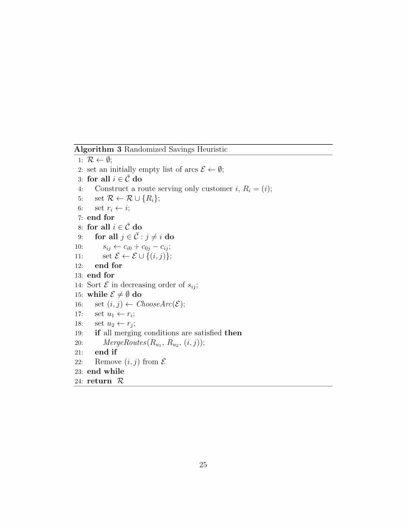
Algorithm 3 shows how the randomized Savings heuristic works. In thisalgorithm, sij denotes the saving of the arc (i, j) and ri denotes the indexof the route serving customer i. An important step of this algorithm is howto choose an arc to merge two routes. In the standard Savings heuristic, ateach iteration the algorithm always chooses the arc with the largest saving.In our implementation we randomly select an arc from the list, based on aprobability assigned to each arc.
For this purpose, we use a geometric distribution during the process: ev-ery time a new arc is selected from the list E of available arcs (which areordered in a decreasing way according to its savings potential), a value ε is
24
Algorithm 3 Randomized Savings Heuristic
1: R ← ∅;2: set an initially empty list of arcs E ← ∅;3: for all i ∈ C do4: Construct a route serving only customer i, Ri = (i);5: set R ← R∪ Ri;6: set ri ← i;7: end for8: for all i ∈ C do9: for all j ∈ C : j 6= i do
10: sij ← ci0 + c0j − cij;11: set E ← E ∪ (i, j);12: end for13: end for14: Sort E in decreasing order of sij;15: while E 6= ∅ do16: set (i, j)← ChooseArc(E);17: set u1 ← ri;18: set u2 ← rj;19: if all merging conditions are satisfied then20: MergeRoutes(Ru1 , Ru2 , (i, j));21: end if22: Remove (i, j) from E23: end while24: return R
25

Algorithm 4 ChooseArc(E)
1: ε← GenerateRandomValue(0.05, 0.25);2: RdmV alue← GenerateRandomValue(0, 1);3: n← 0;4: arcPr ← 0;5: cumPr ← 0;6: for all e ∈ E do7: arcPr ← ε (1− ε)n;8: cumPr ← cumPr + arcPr;9: if RdmV alue < cumPr then
10: return e;11: else12: n← n+ 1;13: end if14: end for15: Choose randomly an arc e from E ;16: return e;
drawn from a uniform distribution on [a, b]. The value of ε is the parameterof the geometric distribution that will be used to assign exponentially dimin-ishing probabilities to each arc according to its position in the list [16, 28].Hence, arcs with larger savings will have a higher probability of being se-lected than those with smaller savings. Algorithm 4 shows the procedure weuse to choose an arc at each iteration.
Note that when using a geometric distribution, a very large number ofarcs in the list E might be required for the cumulative probability to convergeto one. Since the size of E is finite and becomes smaller at each iteration,we might reach the end of the list without finding an arc with the proper cu-mulative probability (Algorithm 4, line 9). In this case, we simply randomlychoose an arc from the list (Algorithm 4, line 15). In our experiments, weuse the interval [0.05, 0.25] to draw the values of the parameter ε.
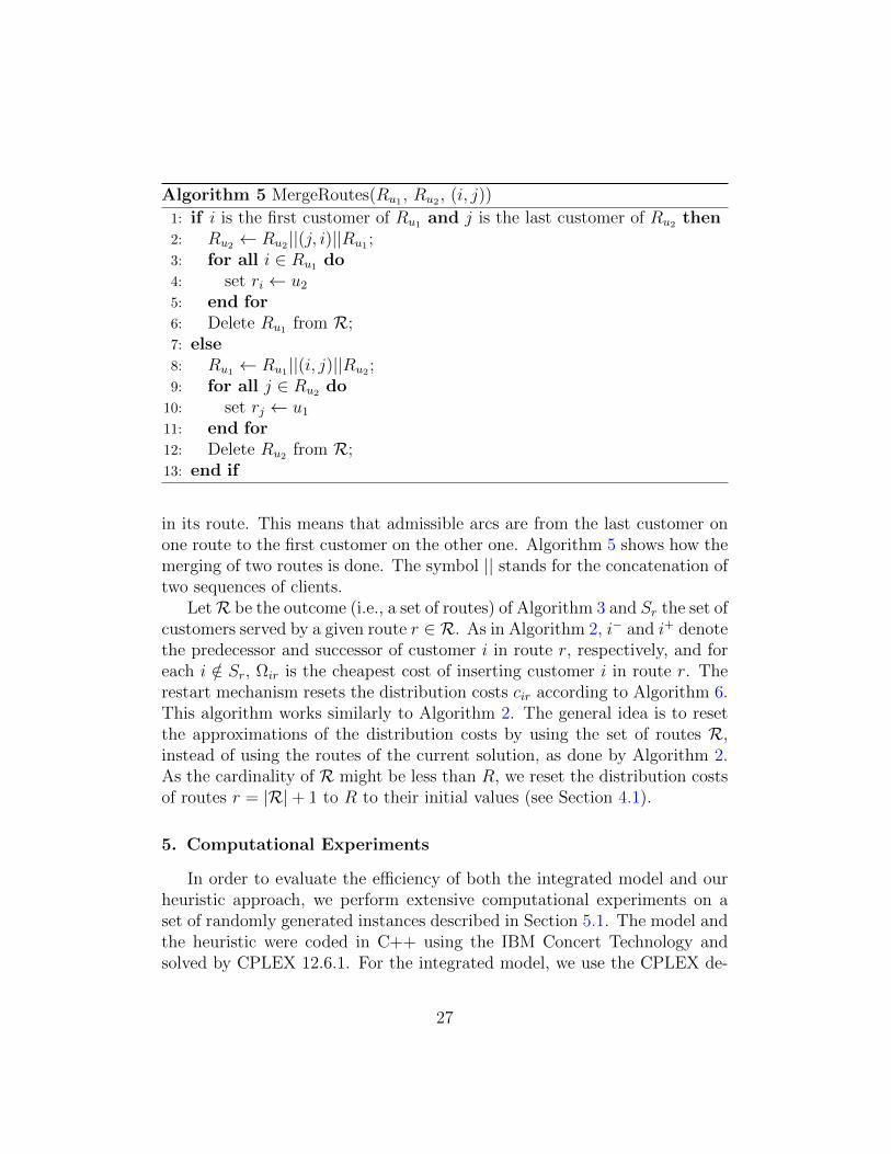
After selecting an arc it is necessary to verify if all the conditions formerging are met. In this step, besides the vehicle capacity constraints, wealso need to take into account the time window constraints. Due to thepresence of time windows, we must account for route orientation. Two partialroutes serving customers i and j, respectively, have compatible orientationsif i is the first (last) customer in its route, and j is the last (first) customer
26
Algorithm 5 MergeRoutes(Ru1 , Ru2 , (i, j))
1: if i is the first customer of Ru1 and j is the last customer of Ru2 then2: Ru2 ← Ru2||(j, i)||Ru1 ;3: for all i ∈ Ru1 do4: set ri ← u2
5: end for6: Delete Ru1 from R;7: else8: Ru1 ← Ru1||(i, j)||Ru2 ;9: for all j ∈ Ru2 do
10: set rj ← u1
11: end for12: Delete Ru2 from R;13: end if
in its route. This means that admissible arcs are from the last customer onone route to the first customer on the other one. Algorithm 5 shows how themerging of two routes is done. The symbol || stands for the concatenation oftwo sequences of clients.
LetR be the outcome (i.e., a set of routes) of Algorithm 3 and Sr the set ofcustomers served by a given route r ∈ R. As in Algorithm 2, i− and i+ denotethe predecessor and successor of customer i in route r, respectively, and foreach i /∈ Sr, Ωir is the cheapest cost of inserting customer i in route r. Therestart mechanism resets the distribution costs cir according to Algorithm 6.This algorithm works similarly to Algorithm 2. The general idea is to resetthe approximations of the distribution costs by using the set of routes R,instead of using the routes of the current solution, as done by Algorithm 2.As the cardinality of R might be less than R, we reset the distribution costsof routes r = |R|+ 1 to R to their initial values (see Section 4.1).
5. Computational Experiments
In order to evaluate the efficiency of both the integrated model and ourheuristic approach, we perform extensive computational experiments on aset of randomly generated instances described in Section 5.1. The model andthe heuristic were coded in C++ using the IBM Concert Technology andsolved by CPLEX 12.6.1. For the integrated model, we use the CPLEX de-
27
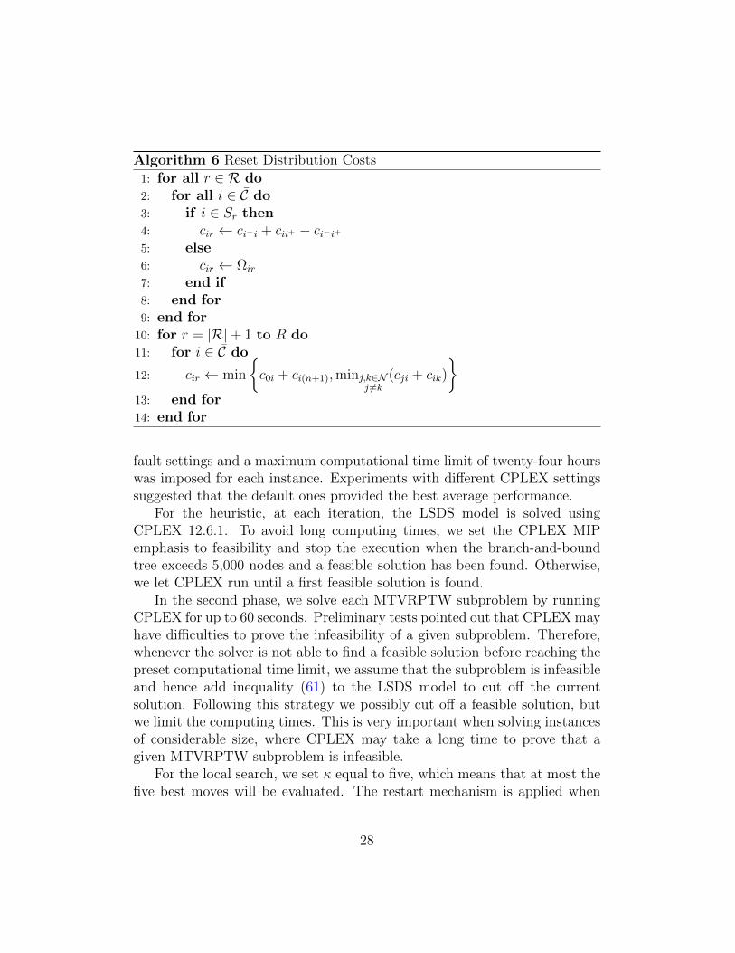
Algorithm 6 Reset Distribution Costs
1: for all r ∈ R do2: for all i ∈ C do3: if i ∈ Sr then4: cir ← ci−i + cii+ − ci−i+5: else6: cir ← Ωir
7: end if8: end for9: end for
10: for r = |R|+ 1 to R do11: for i ∈ C do
12: cir ← min
c0i + ci(n+1),minj,k∈N
j 6=k(cji + cik)
13: end for14: end for
fault settings and a maximum computational time limit of twenty-four hourswas imposed for each instance. Experiments with different CPLEX settingssuggested that the default ones provided the best average performance.
For the heuristic, at each iteration, the LSDS model is solved usingCPLEX 12.6.1. To avoid long computing times, we set the CPLEX MIPemphasis to feasibility and stop the execution when the branch-and-boundtree exceeds 5,000 nodes and a feasible solution has been found. Otherwise,we let CPLEX run until a first feasible solution is found.
In the second phase, we solve each MTVRPTW subproblem by runningCPLEX for up to 60 seconds. Preliminary tests pointed out that CPLEX mayhave difficulties to prove the infeasibility of a given subproblem. Therefore,whenever the solver is not able to find a feasible solution before reaching thepreset computational time limit, we assume that the subproblem is infeasibleand hence add inequality (61) to the LSDS model to cut off the currentsolution. Following this strategy we possibly cut off a feasible solution, butwe limit the computing times. This is very important when solving instancesof considerable size, where CPLEX may take a long time to prove that agiven MTVRPTW subproblem is infeasible.
For the local search, we set κ equal to five, which means that at most thefive best moves will be evaluated. The restart mechanism is applied when
28

Demand of product p at customer i dpi ∈ U [10, 100]Units of item a per unit of product p ηap ∈ U [0, 5]Width (Wa) and length (La) of item a Wa, La ∈ U [5, 10]Coordinates of node i (Xi, Yi) ∈ [0, 500]Initial (minimum) stock of item a Ia0 = Imin
a = 0Unit processing time of item a ρa = 1Unit weight of product p ϕp = 1
Production capacity in period t Kt =
⌈∑a∈C ρa(
∑p∈P
∑i∈N dpiηap)
0.6·|T |
⌉Setup time between items a and b ςab ∈ U [6, 10] if a 6= b, 0 otherwise
Travel time from nodes i to node j τij =
⌈6080
(√(Xi −Xj)
2 + (Yi − Yj)2
)⌉Capacity of vehicle v θv =
⌈U [0.25, 0.50] ·
∑p∈P
∑i∈N dpi · ϕp
⌉Time window of node i ∈
0, C
in period t[δit, δit
]= [480 + 1440 (t− 1) , 1080 + 1440 (t− 1)]
Time window of node n+ 1 in period t[δ(n+1)t, δ(n+1)t
]= [1440 (t− 1) , 1440t]
Time to load/unload per unit of weight λ = 1/50Due date of customer i ∈ C ∆i = δi|T |Maximum number of routes over the planning horizon R = nUnit inventory holding cost of item a ha = 0.001 ·Wa · LaSetup cost of a changeover from item a to item b cab = 25 · ςabTravel cost from node i to node j cij =
⌈√(Xi −Xj)
2 + (Yi − Yj)2
⌉Table 1: Parameters used to generate random instances.
the best solution found so far has not been improved for five consecutiveiterations, and the whole procedure is stopped after the restart mechanismhas been applied five times.
All the experiments were executed on computers with two Intel Xeon 3.07GHz processors and 96 GB of memory.
5.1. Instances Generation
We generated a set of random instances following an approach similarto the one proposed by Gramani et al. [26], for a cutting stock problem,and Armentano et al. [8], for a multi-product PRP. The number of finalproducts (|P|), items (|C|), customers (n) and vehicles (|V|) are chosen inthe sets 3, 5, 3, 5, 10, 15, 20, 30, 40, 50 and 2, 3, respectively.The planning horizon is fixed to 8 periods for all the instances. We generatefive instances for each combination of final products, items, customers andvehicles, resulting in a total of 240 instances. Table 1 presents how theremaining parameters were generated.
Observe that we defined the width and length for each item a in orderto estimate inventory holding costs as a function of the size of the items. Itmeans that the larger a given item is, the more expensive it is to hold it instock. The overall production capacity usage is defined to be around 60%,
29

following the work of Amorim et al. [6]. For the time windows generation, weassume that customers may be visited at any time within regular businesshours, vehicles must also leave the depot within regular working hours, butthey may return at any time. Furthermore, since we considered a relativelyshort planning horizon (8 days), we supposed that the customer deadlinesmatch the end of the last time windows. The time to load/unload per unitof weight was set to 1/50 min/kg, which implies that fifty kilograms areloaded/unloaded in one minute. Finally, we set the upper bound on thenumber of routes as the number of customers in the problem.
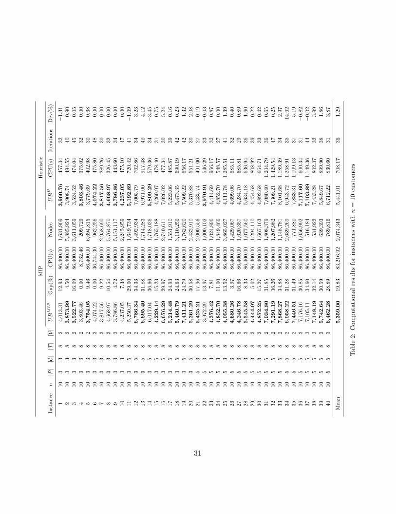
5.2. Numerical Results
In this section we present the computational results on the random in-stances described in Section 5.1. Tables 2–7 compare results achieved bythe integrated model and our decomposition heuristic. All the columns areself-explanatory, except for column “Dev(%)”, which reports the relative de-viation from the CPLEX solutions. Each entry is calculated as:
Dev(%) =UBH − UBMIP
UBMIP× 100,
where UBMIP denotes the total cost of the best solution found by CPLEXand UBH is the total cost of the best solution found by the decompositionheuristic. Negative entries correspond to instances where our heuristic founda better solution than CPLEX.
In general, after 24 hours of computing time, CPLEX is not able to solvemost of the instances. Indeed, only two instances with 10 customers weresolved optimally (see instances 4 and 6 in Table 2). This suggests that, evenafter long runtimes, proving the optimality of a given solution is difficult.The main reason for it is the weakness of the lower bounds provided bythe formulation. Except for a few instances with n = 10 customers, theoptimality gaps are large and, therefore, reaching a guarantee of optimality isunlikely. Furthermore, the weak lower bounds make it difficult to accuratelymeasure the quality of the solutions provided by CPLEX. In some cases,CPLEX may have found an optimal solution but it is not able to prove itbecause of the poor quality of the lower bounds. This is the case, for example,for the sixth instance with 10 customers, whose optimal solution was foundin less than one hour, but the solver took more than ten hours to prove it.
Another drawback of solving the integrated model is that CPLEX is notable to provide feasible solutions for most of the instances with 30 or more
30
MIP
Heu
rist
ic
Inst
ance
n|P||C||T||V|
UBMIP
Gap
(%)
CP
U(s
)N
odes
UBH
CP
U(s
)It
erat
ions
Dev
(%)
110
33
82
4,01
3.31
12.9
386,4
00.0
01,
631,9
093,960.76
457.
3432
−1.
312
103
38
23,873.99
4.50
86,
400.0
05,
885,9
243,9
08.7
449
4.5
540
0.9
03
103
38
23,522.77
16.0
986,4
00.0
03,
611,0
593,5
24.5
247
4.0
445
0.0
54
10
33
82
3,80
3.4
60.0
08,
732.4
620
9,72
93,803.46
375.0
232
0.0
05
103
38
23,754.05
9.4
686,4
00.0
06,
694,8
153,7
79.6
940
2.9
830
0.6
86
103
38
34,
074.2
20.0
036,7
44.3
096
2,25
64,074.22
475.8
048
0.0
07
10
33
83
3,817.5
69.2
286,4
00.0
02,
958,6
903,817.56
289.2
630
0.0
08
103
38
34,
668.9
710
.54
86,4
00.0
05,
764,8
704,668.97
326.4
532
0.0
09
10
33
83
3,78
6.8
64.7
286,
400.0
05,
151,1
173,786.86
443.6
034
0.0
010
10
33
83
4,23
7.0
57.3
886,
400.0
02,
245,9
594,237.05
475.1
047
0.0
011
10
35
82
5,25
0.3
729.0
086,4
00.0
01,
649,7
34
5,192.89
720.4
241
−1.0
912
10
35
82
6,786.34
34.3
386,4
00.0
01,
492,9
347,0
05.7
976
2.8
634
3.2
313
10
35
82
6,695.40
31.8
886,4
00.0
01,
714,2
836,9
71.0
091
7.4
840
4.1
214
103
58
26,
017.0
436
.66
86,4
00.0
01,
718,0
365,809.29
579.3
634
−3.4
515
103
58
24,229.14
15.
2386,4
00.0
01,
765,1
884,2
60.9
747
8.4
031
0.7
516
103
58
36,676.29
29.9
786,
400.0
02,
740,6
11
7,0
26.0
247
7.3
430
5.2
417
10
35
83
5,214.48
24.9
386,4
00.0
01,
551,9
105,2
23.0
648
5.8
739
0.1
618
10
35
83
5,460.79
24.6
386,4
00.0
03,
110,2
505,4
73.3
569
0.1
942
0.2
319
10
35
83
7,411.21
24.7
986,4
00.0
01,
762,6
207,5
09.2
2656
.17
421.3
220
10
35
83
5,261.29
30.5
886,4
00.0
02,
432,9
105,3
70.8
855
1.2
130
2.0
821
10
53
82
5,425.21
17.9
686,4
00.0
02,
000,5
565,4
35.7
449
1.0
027
0.1
922
105
38
23,
972.2
913
.97
86,4
00.0
01,
000,1
023,970.91
546.2
933
−0.0
323
105
38
24,376.42
7.8
186,4
00.0
01,
024,8
964,4
14.6
996
6.1
732
0.8
724
10
53
82
4,852.70
11.0
086,4
00.0
01,
849,4
664,8
52.7
054
8.5
727
0.0
025
105
38
24,055.38
13.5
286,4
00.0
03,
865,0
274,1
11.7
81,
285.5
141
1.3
926
10
53
83
4,680.26
3.9
786,4
00.0
01,
429,0
674,6
99.0
6685
.11
320.4
027
10
53
83
4,246.78
16.6
686,4
00.0
01,
620,3
574,2
84.7
068
5.8
129
0.8
928
10
53
83
5,545.58
8.3
386,4
00.0
01,
077,5
605,6
34.1
863
6.9
436
1.6
029
10
53
83
4,444.97
5.0
286,4
00.0
01,
294,1
104,4
54.6
880
8.9
239
0.2
230
105
38
34,872.25
15.2
786,
400.0
01,
667,1
63
4,8
92.6
866
4.7
133
0.4
231
10
55
82
7,034.80
31.8
586,4
00.0
01,
808,3
797,0
80.4
01,
204.7
936
0.6
532
105
58
27,291.19
36.2
686,
400.0
01,
207,9
827,3
09.2
11,
429.5
447
0.2
533
105
58
27,868.27
34.
8886,4
00.0
01,
148,7
818,1
01.6
81,
189.3
934
2.9
734
10
55
82
6,058.22
31.2
886,4
00.0
02,
639,2
696,9
43.7
21,
258.9
135
14.6
235
10
55
82
7,446.51
31.4
986,4
00.0
077
1,880
7,8
33.3
11,
109.1
337
5.1
936
105
58
37,
176.1
630
.85
86,4
00.0
01,
056,9
927,117.60
600.3
431
−0.8
237
10
55
83
7,10
5.1
134
.60
86,
400.0
051
6,18
47,103.89
1,1
49.3
644
−0.0
238
10
55
83
7,148.19
32.1
486,4
00.0
0531,9
227,4
33.2
8802
.37
323.9
939
10
55
83
5,742.64
30.5
986,4
00.0
063
9,39
35,8
49.6
7899
.90
381.8
640
10
55
83
6,462.28
28.8
986,4
00.0
076
9,81
66,7
12.2
283
0.6
031
3.8
7
Mea
n5,359.00
19.8
383,2
16.9
22,
074,3
43
5,4
41.0
1708
.17
36
1.2
9
Tab
le2:
Com
pu
tati
on
al
resu
lts
for
inst
an
ces
wit
hn
=10
cust
om
ers
31

MIP
Heu
rist
ic
Inst
ance
n|P||C||T||V|
UBMIP
Gap
(%)
CP
U(s
)N
odes
UBH
CP
U(s
)It
erat
ions
Dev
(%)
4115
33
82
3,890.65
20.8
186,4
00.
002,
613,9
103,9
64.3
536
9.9
432
1.8
942
153
38
25,
625.7
820
.78
86,
400.
00
2,87
7,4
805,602.20
565.
8435
−0.
4243
15
33
82
4,741.37
17.3
186,4
00.0
045
1,27
04,8
63.5
836
7.9
333
2.5
844
153
38
25,392.16
13.9
786,4
00.0
045
9,21
25,5
29.3
454
8.1
631
2.5
445
15
33
82
5,13
4.4
024
.82
86,
400.
0042
6,45
04,999.58
916.4
341
−2.6
346
15
33
83
5,228.28
26.2
886,4
00.0
02,
018,
792
5,3
03.2
784
6.0
940
1.4
347
153
38
35,
295.3
517
.00
86,4
00.0
0823,5
505,295.35
479.3
331
0.0
048
153
38
35,768.05
14.3
886,4
00.0
099
4,88
65,7
78.3
834
6.9
632
0.1
849
153
38
35,945.70
12.2
686,
400.0
062
5,68
35,9
54.1
254
2.9
243
0.1
450
15
33
83
4,72
5.6
510
.58
86,4
00.0
082
9,43
54,720.06
504.2
940
−0.1
251
15
35
82
7,725.78
41.8
486,4
00.0
0152,5
377,9
03.2
51,
056.8
831
2.3
052
15
35
82
5,81
1.9
539
.00
86,
400.0
01,
670,8
155,500.22
1,0
49.0
037
−5.3
653
15
35
82
4,870.16
42.7
586,4
00.0
070,
471
4,9
73.0
451
6.8
436
2.1
154
15
35
82
5,62
6.9
137
.39
86,4
00.0
016
7,75
25,582.66
1,6
47.2
645
−0.7
955
15
35
82
5,94
6.1
738
.41
86,
400.0
010
8,33
95,709.59
504.5
330
−3.9
856
15
35
83
7,41
8.6
038
.51
86,4
00.0
067,
361
6,955.31
491.2
230
−6.2
457
15
35
83
7,31
0.3
940.8
686,4
00.0
0183,7
447,305.61
960.7
933
−0.0
758
153
58
37,
017.2
036
.85
86,4
00.0
0249,8
816,858.64
830.7
834
−2.2
659
153
58
36,
436.7
043
.68
86,4
00.0
060,7
256,270.49
766.8
836
−2.5
860
153
58
35,931.46
33.3
386,
400.0
052
7,51
05,9
94.9
71,
353.1
336
1.0
761
155
38
26,021.58
22.
3586,
400.0
061
9,73
26,0
71.0
11,
045.1
937
0.8
262
155
38
25,
076.9
820
.56
86,4
00.0
01,
068,6
405,048.38
1,7
78.9
852
−0.5
663
15
53
82
5,688.68
23.4
886,4
00.0
015
3,03
25,7
09.6
81,
028.8
940
0.3
764
15
53
82
6,631.85
17.4
086,4
00.0
024
8,25
76,8
94.1
8745
.13
333.9
665
15
53
82
6,312.77
20.7
286,4
00.0
01,
818,2
136,3
61.2
31,
897.4
634
0.7
766
15
53
83
6,089.43
26.8
786,4
00.0
01,
350,3
466,1
45.4
31,
433.9
245
0.9
267
15
53
83
5,769.2
217
.69
86,4
00.0
055
1,10
55,769.22
1,2
57.8
230
0.0
068
155
38
35,
657.1
627
.40
86,4
00.0
017
0,00
85,445.72
739.8
833
−3.7
469
15
53
83
4,115.19
8.2
886,4
00.0
01,
355,5
284,1
17.3
885
4.2
435
0.0
570
15
53
83
4,57
7.9
99.4
786,4
00.0
027
4,99
14,577.99
1,0
98.2
236
0.0
071
15
55
82
8,270.59
40.1
886,4
00.0
011
0,03
68,2
77.1
31,
285.2
936
0.0
872
15
55
82
7,76
5.4
834
.75
86,
400.0
012
3,73
27,758.50
1,4
02.9
239
−0.0
973
15
55
82
8,123.29
40.6
386,4
00.0
0111,4
808,1
36.0
11,
298.6
836
0.1
674
15
55
82
8,157.0
334
.51
86,4
00.0
089,4
128,143.78
3,0
09.8
746
−0.1
675
15
55
82
8,13
0.9
042
.33
86,4
00.0
012
0,19
17,812.74
2,5
72.0
736
−3.9
176
15
55
83
5,903.06
35.9
586,4
00.0
0129,1
085,9
19.3
02,
104.3
442
0.2
877
15
55
83
8,249.3
939
.05
86,4
00.0
042,1
848,042.92
3,2
96.2
142
−2.5
078
155
58
39,
071.7
341
.00
86,4
00.0
076,6
038,367.62
1,4
44.6
938
−7.7
679
15
55
83
8,32
3.0
438
.88
86,
400.0
012
4,17
08,252.95
1,0
34.5
137
−0.8
480
15
55
83
7,30
1.5
939
.40
86,
400.0
076,
492
7,261.40
2,5
02.0
742
−0.5
5
Mea
n6,
276.
99
28.7
986,4
00.0
059
9,82
76229.41
1,16
2.39
37−
0.57
Tab
le3:
Com
pu
tati
on
al
resu
lts
for
inst
an
ces
wit
hn
=15
cust
om
ers
32

MIP
Heu
rist
ic
Inst
ance
n|P||C||T||V|
UBMIP
Gap
(%)
CP
U(s
)N
odes
UBH
CP
U(s
)It
erat
ions
Dev
(%)
8120
33
82
6,0
46.9
217.8
486,4
00.0
046
0,33
36,046.92
824.0
237
0.0
082
203
38
27,3
39.5
344.5
786,4
00.0
020,5
435,668.56
1,1
72.5
155
−22.7
783
203
38
25,4
89.2
636.3
286,4
00.0
047,9
015,288.71
532.5
132
−3.6
584
203
38
25,6
12.4
540.8
386,4
00.0
031,4
785,230.07
1,2
42.3
943
−6.8
185
203
38
25,9
14.0
436.6
486,4
00.0
047,4
255,596.14
1,3
48.8
140
−5.3
886
203
38
36,2
86.9
518.9
186,4
00.0
035
6,81
06,084.90
481.1
832
−3.2
187
20
33
83
6,175.56
23.7
386,4
00.0
044
2,27
36,
236.
9976
5.52
410.9
988
203
38
35,7
65.1
329.6
586,4
00.0
062,2
615,393.28
478.4
930
−6.4
589
203
38
35,5
05.5
833.9
986,4
00.0
051,8
595,144.40
510.8
843
−6.5
690
203
38
36,1
74.5
229.8
786,4
00.0
01,
195,4
816,040.64
821.8
642
−2.1
791
203
58
2–
–86
,400
.00
33,4
887,528.84
1,2
28.7
540
–92
203
58
2–
–86
,400
.00
45,4
396,844.97
1,9
02.7
340
–93
203
58
27,0
39.2
034.5
786,4
00.0
079,2
907,017.57
1,0
01.9
738
−0.3
194
20
35
82
––
86,4
00.0
089,9
977,030.76
1,4
43.9
034
–95
203
58
28,4
98.1
139.3
086,4
00.0
059,5
707,780.75
1,1
46.4
633
−8.4
496
203
58
3–
–86
,400
.00
16,5
148,835.16
707.9
231
–97
203
58
37,9
31.2
542.7
686,4
00.0
011
4,87
07,706.05
1,7
79.3
741
−2.8
498
203
58
39,3
69.8
240.4
586,4
00.0
034,1
019,277.08
1,3
43.5
329
−0.9
999
203
58
38,323.71
44.3
586,4
00.0
061,1
898,
431.
571,2
14.4
134
1.3
010
020
35
83
––
86,4
00.0
040,0
097,636.18
1,8
44.4
930
–10
120
53
82
7,9
36.4
044.2
986,4
00.0
026,5
046,386.26
1,45
7.8
242
−19.5
310
220
53
82
8,1
37.0
635.9
586,4
00.0
018
9,38
67,930.72
2,95
0.0
750
−2.5
4103
205
38
26,9
09.3
336.7
086,4
00.0
034,2
756,104.78
1,15
6.9
434
−11.6
410
420
53
82
7,5
14.0
842.3
486,4
00.0
016,8
026,580.70
2,11
8.1
244
−12.4
210
520
53
82
6,6
88.1
337.3
086,4
00.0
045,5
026,252.63
4,49
4.1
349
−6.5
1106
205
38
38,0
94.1
839.5
986,4
00.0
031,8
837,331.90
5,44
6.3
041
−9.4
210
720
53
83
6,2
80.9
545.0
186,4
00.0
028,8
945,312.95
1,65
0.9
830
−15.4
110
820
53
83
7,1
02.1
434.8
286,4
00.0
036,3
026,627.72
1,28
4.9
031
−6.6
810
920
53
83
6,8
87.8
338.1
686,4
00.0
085,1
296,520.65
815.7
127
−5.3
311
020
53
83
7,7
84.9
734.0
586,4
00.0
020
3,83
07,276.56
1,55
1.9
733
−6.5
311
120
55
82
9,8
32.0
241.8
786,4
00.0
031,4
449,330.25
2,51
9.4
627
−5.1
011
220
55
82
11,4
89.5
037.0
286,4
00.0
021,9
2510,847.60
1,88
2.4
239
−5.5
911
320
55
82
––
86,4
00.0
027,3
0211,770.51
5,3
36.0
938
–11
420
55
82
8,7
84.1
645.5
986,4
00.0
011,0
658,027.25
2,02
2.5
040
−8.6
211
520
55
82
––
86,4
00.0
08,
125
8,641.82
2,3
44.1
845
–11
620
55
83
11,8
31.5
037.8
786,4
00.0
039,5
1610,892.61
2,71
4.8
737
−7.9
411
720
55
83
11,8
91.0
047.5
986,4
00.0
07,
051
10,432.21
5,81
5.7
647
−12.2
711
820
55
83
12,3
91.9
039.8
786,4
00.0
022,5
0310,850.02
2,96
4.4
039
−12.4
411
920
55
83
9,8
67.5
528.7
986,4
00.0
070,7
349,531.67
2,30
8.2
750
−3.4
012
020
55
83
13,2
35.7
047.1
386,4
00.0
015,0
4211,432.56
3,63
8.7
146
−13.6
2
Mea
n8,
003.
9537.2
086,4
00.0
010
6,10
17,572.52
1,9
06.6
338
−7.0
4
Tab
le4:
Com
pu
tati
on
al
resu
lts
for
inst
an
ces
wit
hn
=20
cust
om
ers
33

MIP
Heu
rist
ic
Inst
ance
n|P||C||T||V|
UBMIP
Gap
(%)
CP
U(s
)N
odes
UBH
CP
U(s
)It
erati
ons
Dev
(%)
121
30
33
82
––
86,4
00.0
02,
741
6,725.48
2,23
7.4
834
–122
30
33
82
8,3
95.6
637.8
386,4
00.0
038,2
277,816.30
3,262.1
731
−6.9
0123
30
33
82
––
86,4
00.0
03,
399
7,792.07
2,60
7.45
40
–12
430
33
82
––
86,4
00.0
02,
461
7,304.30
2,86
7.76
33–
125
30
33
82
––
86,4
00.0
04,
390
7,538.67
2,451.
8028
–126
30
33
83
8,5
71.6
054.2
486,4
00.0
06,
044
6,035.92
2,82
8.92
33
−29.
5812
730
33
83
––
86,4
00.0
05,
554
8,491.91
3,570.7
127
–128
303
38
3–
–86
,400
.00
2,81
07,825.10
2,356.4
730
–129
30
33
83
––
86,4
00.0
03,
579
6,670.72
3,65
9.49
30
–13
030
33
83
––
86,4
00.0
04,
012
6,297.16
3,5
54.
6938
–13
130
35
82
––
86,4
00.0
01,
926
9,691.07
3,1
04.2
833
–13
230
35
82
––
86,4
00.0
03,
186
10,830.62
3,2
79.9
328
–13
330
35
82
––
86,4
00.0
02,
339
9,424.70
5,2
51.7
238
–134
30
35
82
––
86,4
00.0
03,
056
11,346.72
4,4
38.0
731
–135
303
58
2–
–86
,400
.00
4,71
610,639.29
2,8
14.1
926
–13
630
35
83
––
86,4
00.0
01,
647
9,522.54
2,9
19.1
830
–137
30
35
83
––
86,4
00.0
01,
619
11,829.88
4,2
93.4
136
–13
830
35
83
––
86,4
00.0
02,
755
9,992.65
2,8
39.6
626
–139
30
35
83
––
86,4
00.0
02,
607
6,669.65
6,4
42.3
160
–140
303
58
3–
–86
,400
.00
1,97
99,650.25
5,4
08.4
032
–14
130
53
82
––
86,4
00.0
01,
620
10,434.49
3,5
95.5
537
–14
230
53
82
––
86,4
00.0
03,
488
9,843.34
6,7
30.4
241
–143
30
53
82
––
86,4
00.0
02,
315
8,516.00
8,2
82.3
037
–144
30
53
82
––
86,4
00.0
02,
182
7,563.69
1,6
42.5
531
–145
305
38
2–
–86
,400
.00
3,78
28,725.91
6,1
14.8
627
–14
630
53
83
––
86,4
00.0
03,
101
8,102.84
7,9
13.4
531
–14
730
53
83
9,7
27.2
846.5
786,4
00.0
03,
485
8,309.28
6,5
40.9
829
−14.
58148
305
38
3–
–86
,400
.00
1,76
97,830.03
7,1
51.6
532
–149
305
38
3–
–86
,400
.00
1,93
29,546.77
8,9
11.2
833
–15
030
53
83
––
86,4
00.0
03,
442
7,211.02
6,2
33.7
436
–15
130
55
82
––
86,4
00.0
02,
234
11,343.12
4,5
29.6
033
–152
30
55
82
––
86,4
00.0
02,
285
17,289.70
5,9
61.6
926
–153
305
58
2–
–86
,400
.00
1,90
612,138.44
6,2
54.1
934
–154
30
55
82
––
86,4
00.0
02,
737
10,062.16
8,1
78.3
030
–15
530
55
82
––
86,4
00.0
01,
859
12,320.81
7,2
39.0
130
–15
630
55
83
––
86,4
00.0
01,
638
12,638.15
7,2
36.1
928
–157
30
55
83
––
86,4
00.0
01,
843
13,390.47
10,
432.9
032
–158
305
58
3–
–86,4
00.0
01,
700
12,117.37
7,5
84.8
743
–15
930
55
83
––
86,4
00.0
01,
866
12,695.75
9,7
36.2
634
–16
030
55
83
––
86,4
00.0
01,
831
12,465.77
6,5
04.6
346
–
Mea
n8,
898.1
846.2
186,4
00.0
03,
652
9,616.00
5,17
4.0
633
−17.
02
Tab
le5:
Com
pu
tati
on
al
resu
lts
for
inst
an
ces
wit
hn
=30
cust
om
ers
34

MIP
Heu
rist
ic
Inst
ance
n|P||C||T||V|
UBMIP
Gap
(%)
CP
U(s
)N
odes
UBH
CP
U(s
)It
erat
ions
Dev
(%)
161
403
38
2–
–86,4
00.0
03,0
967,433.32
7,1
63.4
031
–16
240
33
82
––
86,4
00.0
01,1
686,932.96
5,0
13.4
555
–16
340
33
82
9,9
74.2
054.5
586,4
00.0
02,0
467,209.82
7,3
84.2
629
−27.7
216
440
33
82
––
86,4
00.0
03,0
968,210.88
10,6
75.6
036
–16
540
33
82
––
86,4
00.0
02,0
357,019.21
6,3
66.8
732
–16
640
33
83
––
86,4
00.0
01,2
887,649.14
6,5
03.5
334
–16
740
33
83
––
86,4
00.0
01,4
498,341.77
12,8
72.7
034
–16
840
33
83
––
86,4
00.0
01,4
358,524.84
8,0
87.5
333
–16
940
33
83
––
86,4
00.0
01,3
187,203.91
9,0
24.6
340
–17
040
33
83
––
86,4
00.0
02,8
987,186.48
5,2
86.1
531
–17
140
35
82
––
86,4
00.0
01,5
0911,795.54
4,9
00.7
330
–17
240
35
82
––
86,4
00.0
01,5
0912,244.95
8,3
29.3
232
–17
340
35
82
––
86,4
00.0
01,5
0911,970.99
8,7
23.1
933
–17
440
35
82
––
86,4
00.0
02,8
4811,568.07
7,0
40.8
126
–17
540
35
82
––
86,4
00.0
095
311,825.04
6,0
15.9
628
–17
640
35
83
––
86,4
00.0
02,5
3012,521.46
7,8
80.9
930
–17
740
35
83
––
86,4
00.0
01,7
6612,948.66
6,2
38.6
337
–17
840
35
83
––
86,4
00.0
02,6
2111,008.08
6,1
36.9
530
–17
940
35
83
––
86,4
00.0
01,2
6211,397.47
10,7
02.8
038
–18
040
35
83
––
86,4
00.0
02,1
418,900.21
11,8
10.1
050
–18
140
53
82
––
86,4
00.0
05,3
3610,599.76
13,7
45.0
041
–18
240
53
82
––
86,4
00.0
01,7
0114,379.70
5,4
24.5
929
–18
340
53
82
––
86,4
00.0
01,8
8514,756.00
17,7
57.6
029
–18
440
53
82
––
86,4
00.0
01,1
4011,431.08
8,6
58.4
928
–18
540
53
82
––
86,4
00.0
04,5
2710,766.61
5,5
34.7
930
–18
640
53
83
––
86,4
00.0
01,1
077,035.79
13,3
89.4
037
–18
740
53
83
––
86,4
00.0
01,4
329,267.54
18,5
07.8
036
–18
840
53
83
––
86,4
00.0
01,7
0211,448.84
13,0
94.8
035
–18
940
53
83
––
86,4
00.0
01,3
0411,696.88
13,9
21.0
039
–19
040
53
83
––
86,4
00.0
01,0
019,185.02
13,2
47.4
039
–19
140
55
82
––
86,4
00.0
02,2
0514,656.10
19,2
89.9
033
–19
240
55
82
––
86,4
00.0
050
114,171.30
16,5
49.4
041
–19
340
55
82
––
86,4
00.0
063
213,393.36
15,9
02.7
039
–19
440
55
82
––
86,4
00.0
03,2
0617,826.20
18,7
82.9
032
–19
540
55
82
––
86,4
00.0
01,8
8516,980.80
13,5
05.5
028
–19
640
55
83
––
86,4
00.0
02,0
1013,883.90
28,9
76.7
043
–19
740
55
83
––
86,4
00.0
060
616,069.40
16,7
75.1
031
–19
840
55
83
––
86,4
00.0
01,1
3212,578.44
14,9
48.2
034
–19
940
55
83
––
86,4
00.0
03,1
2215,037.40
27,8
41.3
038
–20
040
55
83
––
86,4
00.0
01,0
6917,757.10
18,1
97.4
039
–
Mea
n9,
974.2
054.5
586,4
00.0
01,9
0011,370.35
11,7
55.1
935
−27.
72
Tab
le6:
Com
pu
tati
on
al
resu
lts
for
inst
an
ces
wit
hn
=40
cust
om
ers
35

MIP
Heu
rist
ic
Inst
ance
n|P||C||T||V|
UBMIP
Gap
(%)
CP
U(s
)N
odes
UBH
CP
U(s
)It
erat
ions
Dev
(%)
201
503
38
2–
–86
,400.0
01,8
9010,898.45
8,27
7.03
34
–20
250
33
82
––
86,4
00.0
01,4
039,237.78
10,
553.0
033
–20
350
33
82
––
86,4
00.0
053
88,967.56
17,
817.5
027
–20
450
33
82
––
86,4
00.0
02,2
80
9,814.34
8,867.5
930
–20
550
33
82
––
86,4
00.0
01,4
18
8,871.72
6,676.9
626
–20
650
33
83
––
86,4
00.0
053
28,212.02
23,2
51.
7031
–20
750
33
83
––
86,4
00.0
0535
10,637.55
21,1
10.
00
43
–20
850
33
83
––
86,4
00.0
0597
8,348.17
16,
251.
30
42
–20
950
33
83
––
86,4
00.0
01,5
988,174.64
7,97
4.83
36
–21
050
33
83
––
86,4
00.0
01,5
909,603.85
26,
018.
40
31
–21
150
35
82
––
86,4
00.0
03,3
4614,271.50
10,
003.
10
26
–21
250
35
82
––
86,4
00.0
048
913,115.20
15,
222.2
027
–21
350
35
82
––
86,4
00.0
01,4
5011,783.77
9,442.8
735
–21
450
35
82
––
86,4
00.0
049
110,309.82
13,4
02.5
027
–21
550
35
82
––
86,4
00.0
049
010,145.22
14,7
58.
1032
–21
650
35
83
––
86,4
00.0
050
312,107.37
29,6
69.
40
40
–21
750
35
83
––
86,4
00.0
01,0
0915,864.90
13,
940.8
029
–21
850
35
83
––
86,4
00.0
0996
14,254.30
15,
065.5
038
–21
950
35
83
––
86,4
00.0
049
812,302.42
25,5
08.4
026
–22
050
35
83
––
86,4
00.0
01,1
36
12,450.73
15,0
11.
6028
–22
150
53
82
––
86,4
00.0
01,4
8512,825.05
33,6
45.
60
29
–22
250
53
82
––
86,4
00.0
0990
14,168.90
12,
759.6
029
–22
350
53
82
––
86,4
00.0
0990
10,651.21
8,777.8
826
–22
450
53
82
––
86,4
00.0
01,9
80
11,339.20
19,3
27.6
030
–22
550
53
82
––
86,4
00.0
01,9
80
12,661.37
25,0
45.
3033
–22
650
53
83
––
86,4
00.0
051
310,910.71
46,2
29.
60
35
–22
750
53
83
––
86,4
00.0
01,5
398,690.50
51,
364.2
028
–22
850
53
83
––
86,4
00.0
0513
13,548.20
41,
251.7
028
–22
950
53
83
––
86,4
00.0
02,0
52
10,758.28
40,8
76.0
026
–23
050
53
83
––
86,4
00.0
01,5
39
9,613.43
23,0
83.
0033
–23
150
55
82
––
86,4
00.0
051
418,487.90
27,0
27.
40
27
–23
250
55
82
––
86,4
00.0
0526
20,292.90
26,
941.1
026
–23
350
55
82
––
86,4
00.0
01,0
2814,346.60
32,
617.2
030
–23
450
55
82
––
86,4
00.0
052
021,666.70
24,2
58.7
031
–23
550
55
82
––
86,4
00.0
01,0
28
14,724.30
19,4
50.
5033
–23
650
55
83
––
86,4
00.0
01,0
9219,271.10
36,7
01.
90
30
–23
750
55
83
––
86,4
00.0
0538
17,746.30
23,
042.3
035
–23
850
55
83
––
86,4
00.0
0538
18,290.50
47,
300.2
026
–23
950
55
83
––
86,4
00.0
02,6
90
20,743.60
44,2
42.3
028
–24
050
55
83
––
86,4
00.0
053
816,369.70
32,8
21.
1028
–
––
86,4
00.0
01,1
35
12,911.94
23,
139.6
531
–
Tab
le7:
Com
pu
tati
on
al
resu
lts
for
inst
an
ces
wit
hn
=50
cust
om
ers
36

customers. The number of nodes explored in the branch-and-bound treeprovides some insights into the difficulty of solving these instances. Overall,CPLEX is not able to find feasible solutions for most of the instances in whichthe number of nodes explored is very small after 24 hours of computing time(see Tables 5–7). Solving each node of the branch-and-bound tree becomesmuch harder when the size of the problem increases and, therefore, CPLEXcannot explore many nodes during the search.
Regarding our heuristic, results show that it is able to provide competitivesolutions for instances with 10 customers. For these instances, the averagetotal cost of the heuristic solutions is 5,441.01, which represents an averagedeviation of only 1.29% from the CPLEX solutions. However, the heuristicrequires only 0.20 hours of computing time (i.e., 12 minutes), on average, incomparison with the 23.12 hours required by the solver.
For instances with 15 customers, our heuristic provides better results thanCPLEX in shorter computing times. CPLEX reached the computationaltime limit of 24 hours for all the cases (Table 3). The heuristic, on theother hand, just required an average computing time of 0.32 hours (i.e., ≈19minutes) and returned solutions with an average deviation of −0.57%. Inparticular, our heuristic provided better solutions than CPLEX for 19 outof 40 instances, with an average deviation of −2.35%. For the remaining 21instances, where CPLEX obtained better solutions, the average deviation ofthe heuristic solutions was only 1.03%.
For instances with 20 customers the heuristic is clearly superior to CPLEX.The solver did not return any feasible solution for seven out of 40 instances(Table 4), while the heuristic provided feasible solutions for all cases. More-over, it obtained a significant reduction of the total cost for most of theinstances, with an average deviation of −7.04%, requiring approximately 32minutes of computing time, on average.
For instances with n ≥ 30, the performance of CPLEX deteriorates sig-nificantly, while the heuristic is still able to provide solutions within reason-able computational times. In general, the heuristic found feasible solutionsfor all the cases, whereas the solver only found feasible solutions for fourinstances. As described above, instances of these sizes are beyond the cur-rent capabilities of CPLEX, which is not able to explore many nodes in thebranch-and-bound tree before reaching the computational time limit.
Note that the average computing time of the heuristic increases with thesize of the problem, ranging from 0.20 hours, for ten customers, to 6.43 hours,for fifty customers. These times, besides being much shorter than the time
37
required by CPLEX, can be considered acceptable in practical situations,since this kind of integrated problems is usually solved on a weekly basis.Computational experiments pointed out that the main reason for the increasein computing times is the hardness of model LSSD, which needs to be solvedat each iteration of the algorithm. Although this model is smaller than thefull integrated model, it is still difficult to solve and the time required toreach the stopping criterion increases with the size of the problem.
Information related to average costs, computing times, number of itera-tions and feasible solutions found during the execution of the heuristic arepresented in Table 8. We grouped the 240 instances according to the numberof customers (n), items (|C|) and vehicles, which have a direct impact on thesize of the problems. Therefore, each entry of Table 8 represents the averageof ten instances.
Regarding the average number of feasible solutions found during the exe-cution of the algorithm, we observe that it tends to decrease with the size ofthe problem. The larger the instances the more difficult it is for the heuristicto find feasible solutions at each iteration. Nevertheless, we are still ableto provide feasible solutions for the largest instances, where CPLEX cannotfind a single feasible solution after one day of computing time.
Another interesting feature of our heuristic is its robustness. In general,the heuristic is able to provide consistent results over different independentruns. This can be observed not only in terms of the total cost, but alsoin terms of the computing time, deviation percentage, number of iterationsand number of feasible solution solutions found during the execution of thealgorithm. Tables 9 and 10 compare the average results of a single run of theheuristic with the average results of five other independent runs.
These results show the potential for practical application of our heuristic,which achieves good quality solutions within reasonable times for all theinstances, including the ones whose size is not manageable for state-of-the-art commercial solvers.
6. Concluding Remarks and Research Directions
In this paper we proposed a decomposition heuristic to deal with a produc-tion routing problem that takes into account relevant features from make-to-order companies. The heuristic decomposes the problem into two parts thatare then solved in an iterative way. Roughly speaking, the first part takescare of all the production decisions as well as the assignment of customers to
38

n |C| |V| Total Cost Inv.+Setup Routing CPU(h) #Iterations #Feas. Sol.
10 3 2 4,176.30 2,054.60 2,121.70 0.17 34 263 4,455.00 2,207.30 2,247.70 0.15 36 30
5 2 6,650.83 4,392.03 2,258.80 0.27 37 293 6,481.92 4,202.52 2,279.40 0.20 36 29
Average 5,441.01 3,214.11 2,226.90 0.20 36 28
15 3 2 5,504.35 2,932.25 2,572.10 0.26 37 223 5,310.69 2,800.99 2,509.70 0.23 37 26
5 2 6,979.69 4,460.19 2,519.50 0.40 37 213 7,122.92 4,628.62 2,494.30 0.41 37 28
Average 6,229.41 3,705.51 2,523.90 0.32 37 24
20 3 2 6,108.55 3,605.25 2,503.30 0.48 43 273 6,197.00 3,500.50 2,696.50 0.38 35 18
5 2 8,482.03 5,816.83 2,665.20 0.58 37 233 9,502.51 6,607.61 2,894.90 0.68 38 24
Average 7,572.52 4,882.55 2,689.98 0.53 38 23
30 3 2 8,226.03 5,017.43 3,208.60 1.11 34 133 7,632.08 4,380.18 3,251.90 1.46 32 14
5 2 11,508.66 8,259.36 3,249.30 1.42 31 103 11,097.25 7,772.95 3,324.30 1.76 37 18
Average 9,616.00 6,357.48 3,258.53 1.44 33 14
40 3 2 9,873.93 6,525.23 3,348.70 2.44 34 113 8,754.02 5,355.32 3,398.70 3.16 36 14
5 2 13,643.24 10,106.14 3,537.10 3.31 32 83 13,210.21 9,769.71 3,440.50 4.15 37 17
Average 11,370.35 7,939.10 3,431.25 3.27 35 13
50 3 2 10,943.56 7,324.96 3,618.60 4.22 30 73 9,849.74 6,234.44 3,615.30 8.26 33 10
5 2 14,914.39 11,180.79 3,733.60 5.36 29 63 15,940.09 12,163.69 3,776.40 7.87 31 10
Average 12,911.94 9,225.97 3,685.98 6.43 31 8
Table 8: Average results of the heuristics on the random instances
39

10 customers 15 customers 20 customers
1 run 5 runs 1 run 5 runs 1 run 5 runs
Inv.+Setup Cost 3,214.11 3,192.18 3,705.51 3,695.61 4,882.55 4,879.77Routing Cost 2,226.90 2,252.96 2,523.90 2,516.03 2,689.98 2,696.09
Total Cost 5,441.01 5,445.13 6,229.41 6,211.64 7,572.52 7,575.86CPU(h) 0.20 0.18 0.32 0.29 0.53 0.48Dev(%) 1.29 1.35 −0.57 −0.82 −7.04 −7.06
#Iterations 36 35 37 36 38 37#Feas. Sol. 28 28 24 25 23 22
Table 9: Comparison of the average results of the heuristic after five independent runs (10to 20 customers)
30 customers 40 customers 50 customers
1 run 5 runs 1 run 5 runs 1 run 5 runs
Inv.+Setup Cost 6,357.48 6,345.25 7,939.10 7,912.58 9,225.97 9,215.55Routing Cost 3,258.53 3,178.26 3,431.25 3,445.02 3,685.98 3,723.35
Total Cost 9,616.00 9,523.51 11,370.35 11,357.60 12,911.94 12,938.90CPU(h) 1.44 1.43 3.27 2.83 6.43 6.35Dev(%) −17.02 −18.02 −27.72 −27.35 – –
#Iterations 33 35 35 32 31 32#Feas. Sol. 14 15 13 11 8 8
Table 10: Comparison of the average results of the heuristic after five independent runs(30 to 50 customers)
40

routes, without considering routing decisions explicitly. In the second part,the sequence and time of the visits is decided by solving a multi-trip vehiclerouting problem for each vehicle used in the first phase.
Computational experiments showed that CPLEX is capable of solvinginstances with up to twenty customers. For instances with no more thanfifteen customers, the heuristic provided solutions of similar quality to thosereturned by the solver. With twenty customers, it clearly outperformedCPLEX, finding solutions of better quality. In all cases, the heuristic re-quired considerably shorter computing times. In addition, our procedurereturned feasible solutions for instances with up to fifty customers, for whichthe solver could not find any solution within one day of computing time.
As a research perspective, it would be interesting to develop an effec-tive heuristic procedure to solve the LSDS subproblem. This model becomesharder to solve when the size of the problem increases and, therefore, de-veloping efficient ways to solve it is necessary in order to reduce computingtimes on larger instances. Moreover, it would also allow us to perform moreiterations, which may help to find better solutions.
Another interesting idea is to apply Lagrangian Relaxation to the inte-grated model in order to compute good lower bounds, which can be usedto measure the quality of heuristic solutions. Moreover, by applying specificroutines to recover feasibility, new feasible solutions for the original problemmay be found while solving the Lagrangian dual problem.
Acknowledgments
This work was supported by the Sao Paulo Research Foundation (FAPESP)under Grant number 2014/10565-8 and the Brazilian National Council forScientific and Technological Development (CNPq) under Grants numbers140179/2014-3 and 312569/2013-0. This support is gratefully acknowledged.
References
[1] Absi, N., Archetti, C., Dauzere-Peres, S., Feillet, D., 2014. A two-phaseiterative heuristic approach for the production routing problem. Trans-portation Science 49 (4), 784–795.
[2] Adulyasak, Y., Cordeau, J.-F., Jans, R., 2014. Formulations and branch-and-cut algorithms for multivehicle production and inventory routingproblems. INFORMS Journal on Computing 26, 103–120.
41

[3] Adulyasak, Y., Cordeau, J.-F., Jans, R., 2014. Optimization-basedadaptive large neighborhood search for the production routing problem.Transportation Science 48 (1), 20–45.
[4] Adulyasak, Y., Cordeau, J.-F., Jans, R., 2015. Benders decompositionfor production routing under demand uncertainty. Operations Research63 (4), 851–867.
[5] Adulyasak, Y., Cordeau, J.-F., Jans, R., 2015. The production routingproblem: A review of formulations and solution algorithms. Computers& Operations Research 55, 141–152.
[6] Amorim, P., Belo-Filho, M., Toledo, F., Almeder, C., Almada-Lobo, B.,2013. Lot sizing versus batching in the production and distribution plan-ning of perishable goods. International Journal of Production Economics146 (1), 208–218.
[7] Archetti, C., Bertazzi, L., Paletta, G., Speranza, M. G., 2011. Anal-ysis of the maximum level policy in a production-distribution system.Computers & Operations Research 38 (12), 1731–1746.
[8] Armentano, V., Shiguemoto, A., Løkketangen, A., 2011. Tabu searchwith path relinking for an integrated production–distribution problem.Computers & Operations Research 38 (8), 1199–1209.
[9] Bard, J. F., Nananukul, N., 2009. Heuristics for a multiperiod inventoryrouting problem with production decisions. Computers & Industrial En-gineering 57 (3), 713–723.
[10] Bard, J. F., Nananukul, N., 2009. The integrated production–inventory–distribution–routing problem. Journal of Scheduling 12 (3), 257–280.
[11] Bard, J. F., Nananukul, N., 2010. A branch-and-price algorithm foran integrated production and inventory routing problem. Computers &Operations Research 37 (12), 2202–2217.
[12] Bertazzi, L., 2005. Minimizing the total cost in an integrated vendor–managed inventory system. Journal of Heuristics 11, 393–419.
[13] Boudia, M., Louly, M., Prins, C., 2007. A reactive GRASP and pathrelinking for a combined production–distribution problem. Computers& Operations Research 34 (11), 3402–3419.
42
[14] Boudia, M., Prins, C., 2009. A memetic algorithm with dynamic popu-lation management for an integrated production–distribution problem.European Journal of Operational Research 195 (3), 703–715.
[15] Brahimi, N., Aouam, T., 2016. Multi-item production routing problemwith backordering: a milp approach. International Journal of ProductionResearch 54 (4), 1076–1093.
[16] Caceres-Cruz, J., Grasas, A., Ramalhinho, H., Juan, A. A., 2014. Asavings-based randomized heuristic for the heterogeneous fixed fleet ve-hicle routing problem with multi-trips. Journal of Applied OperationalResearch 6 (2), 69–81.
[17] Chandra, P., Fisher, M. L., 1994. Coordination of production and distri-bution planning. European Journal of Operational Research 72, 503–517.
[18] Chen, Z.-L., 2004. Integrated production and distribution operations:taxonomy, models, and review. In: Simchi-Levi, D., Wu, S., Shen, Z.-J.(Eds.), Handbook of quantitative supply chain analysis: modeling in thee-business era. Kluwer Academic Publishers, Ch. 17, pp. 711–745.
[19] Chitsaz, M., , Cordeau, J.-F., Jans, R., 2017. A unified decompositionmatheuristic for assembly, production and inventory routing. Tech. rep.,GERAD G–2017–03, HEC Montreal, Canada.
[20] Clarke, G., Wright, J. W., 1964. Scheduling of vehicles from a centraldepot to a number of delivery points. Operations Research 12, 568–581.
[21] Cordeau, J.-F., Laporte, G., Savelsbergh, M. W., Vigo, D., 2007. Vehiclerouting. In: Barnhart, C., Laporte, G. (Eds.), Transportation. Vol. 14of Handbooks in operations research and management science. Elsevier,Ch. 6, pp. 367–428.
[22] Dıaz-Madronero, M., Peidro, D., Mula, J., 2015. A review of tacticaloptimization models for integrated production and transport routingplanning decisions. Computers & Industrial Engineering 88, 518–535.
[23] Fischetti, M., Lodi, A., 2003. Local branching. Mathematical Program-ming 98 (1), 23–47.
43

[24] Fumero, F., Vercellis, C., 1999. Synchronized development of produc-tion, inventory, and distribution schedules. Transportation Science 33,330–340.
[25] Golden, B. L., Raghavan, S., Wasil, E. A. (Eds.), 2008. The vehicle rout-ing problem: latest advances and new challenges, 1st Edition. SpringerUS, New York.
[26] Gramani, M., Franca, P., Arenales, M., 2009. A lagrangian relaxationapproach to a coupled lot-sizing and cutting stock problem. InternationalJournal of Production Economics 119 (2), 219–227.
[27] Jans, R., Degraeve, Z., 2008. Modeling industrial lot sizing problems: areview. International Journal of Production Research 46 (6), 1619–1643.
[28] Juan, A. A., Faulin, J., Jorba, J., Riera, D., Masip, D., Barrios, B.,2011. On the use of monte carlo simulation, cache and splitting tech-niques to improve the clarke and wright savings heuristics. Journal ofthe Operational Research Society 62 (6), 1085–1097.
[29] Karimi, B., Fatemi Ghomi, S., Wilson, J., 2003. The capacitated lotsizing problem: A review of models and algorithms. Omega 31 (5), 365–378.
[30] Lei, L., Liu, S., Ruszczynski, A., Park, S., 2006. On the integrated pro-duction, inventory, and distribution routing problem. IIE Transactions38 (11), 955–970.
[31] Miranda, P. L., Morabito, R., Ferreira, D., 2016. Optimization modelfor a production, inventory, distribution routing problem in small furni-ture companies. Tech. rep., Production Engineering Department, Fed-eral Univeristy of Sao Carlos, Brazil.
[32] Miranda, P. L., Morabito, R., Ferreira, D., 2017. Mixed integer formula-tions for a coupled lot-scheduling and vehicle routing problem in furni-ture settings. Tech. rep., Production Engineering Department, FederalUniveristy of Sao Carlos, Brazil.
[33] Pochet, Y., Wolsey, L. A., 2006. Production planning by mixed integerprogramming. Springer Science & Business Media.
44

[34] Ruokokoski, M., Solyali, O., Cordeau, J.-F., Jans, R., Sural, H., 2010.Efficient formulations and a branch-and-cut algorithm for a production-routing problem. Tech. rep., GERAD G–2010–66, HEC Montreal,Canada.
[35] Shiguemoto, A. L., Armentano, V. A., 2010. A tabu search procedure forcoordinating production, inventory and distribution routing problems.International Transactions in Operational Research 17 (2), 179–195.
[36] Toth, P., Vigo, D. (Eds.), 2002. The Vehicle Routing Problem, 1st Edi-tion. SIAM, Philadelphia, PA, USA.
45