a decomposition of productivity change in the
TRANSCRIPT
International Journal of Production ResearchVol. 49, No. 16, 15 August 2011, 4761–4785
A decomposition of productivity change in the semiconductor
manufacturing industry
Chia-Yen Lee and Andrew L. Johnson*
Department of Industrial and Systems Engineering, Texas A&M University,College Station, TX 77840, USA
(Received 4 November 2009; final version received 23 April 2010)
This study divides a production system into three components: production design,demand support, and operations. Efficiency is then decomposed via network dataenvelopment analysis and integrated into the Malmquist Productivity Indexframework to develop a more detailed decomposition of productivity change.The proposed model can identify the demand effect and the identity of the rootcause of technical regress. Specifically, the demand effect allows the source oftechnical regress to be attributed to both demand deterioration and technicalregress in the production technology. An empirical study using data from 1995 to2000 for the semiconductor manufacturing industry is presented to demonstrateand validate the proposed method. The result shows that the regress ofproductivity in 1997–1998 and 1999–2000 is mainly caused by demand fluctu-ations rather than by technical regression in production capabilities.
Keywords: productivity change; efficiency decomposition; MalmquistProductivity Index; semiconductor manufacturing
1. Introduction
In manufacturing processes, productivity analysis is a technique used to assessperformance and to search for improvement alternatives. The efficient frontier can beconstructed to characterise how efficiently production processes use inputs to generateoutputs; given the same input resource, inefficiency is indicated by lower levels of systemoutput. However, in practice, the decrease of actual output sometime results frominsufficient demand. Demand fluctuations can bias productivity analysis. Similarly, inpanel data analysis, the Malmquist Productivity Index (MPI) quantifies efficiency changeand technology change over time. Technical regress is often attributed to productionissues, when in reality it may be a result of demand deterioration. Thus, productivityanalysis attributes changes in demand to production. The proposed model in this studycan separate the demand effect and production technology effect to eliminate the biasinterpretation of efficiency.
There is a limited literature discussing the effects of demand in productivity analysis.Fielding et al. (1985) study the performance evaluation of transportation systems. Theydistinguish between the production process and the consumption process, arguing thatoutput consumption is substantially different from output production since transportation
*Corresponding author. Email: [email protected]
ISSN 0020–7543 print/ISSN 1366–588X online
� 2011 Taylor & Francis
DOI: 10.1080/00207543.2010.497507
http://www.informaworld.com
Dow
nloa
ded
by [
Tex
as A
&M
Uni
vers
ity L
ibra
ries
] at
20:
49 2
4 N
ovem
ber
2014
services cannot be stored. They propose various performance indicators, specifically,service effectiveness, which is the ratio of passenger trip miles over vehicle operating miles.However, single factor productivity indicators do not represent all factors in theproduction system (Chen and McGinnis 2007). Lan and Lin (2005) and Yu and Lin (2008)use data envelopment analysis (DEA) and network DEA models to characterise aconsumption process. However, demand and production processes characterised intransportation are different from the manufacturing industry, where manufacturerscommonly depend on forecasted or contract demand based on expected sales or actualsales respectively. Longer production lead times require an ‘internal’ demand-supportingprocess; in contrast, transportation companies mainly rely on non-contract demandrequested informally by customers after production, and the services must be consumed bycustomers immediately or they are no longer useful. We note, too, that previous studiesfocus on a cross-sectional analysis and do not provide estimates of productivity changeover time.
Change in demand can also effect the measurement of productivity changes over timeas estimated through frontier shifts indicating either technical progress or regress.Nishimizu and Page (1982) propose the first decomposition of total factor productivitychange, and Fare et al. (1992, 1994) develop the explicit measurement of productivitychange based on the MPI proposed by Caves et al. (1982), which uses Shephard’s inputdistance function (Shephard 1953) to estimate inefficiency non-parametrically. Theproductivity change estimated via MPI can be decomposed into two sub-indices: change inefficiency and change in technology. This decomposition provides useful information inindustrial application. Fare et al. (1992) apply the change in scale decomposition toSwedish pharmacies between 1980–1989, finding that during the latter part of the 1980sthe positive productivity change is mainly due to shifts of frontier rather than changes inefficiency. In another study, 17 OECD (Organisation for Economic Cooperation andDevelopment) countries are analysed in terms of gross domestic product, capital stock,and labour between 1979 and 1988 and an additional scale component is introduced(Fare et al. 1994). The results show that all of the productivity growth is chiefly due totechnical change, with Japan having the highest productivity growth. Chang et al. (2008),who analyse performance evaluation in printed circuit board manufacturers between 2002and 2003, find that manufacturing processes with lower efficiency and a lower MPI shouldbe suggested for outsourcing, because they cause low capacity utilisation of expensiveequipment. Several researchers develop further decomposition of productivity change,e.g. Tulkens and Vanden Eeckaut (1995), Ray and Desli (1997), Sueyoshi and Aoki (2001),Sueyoshi and Goto (2001) and Lovell (2003).
Other studies evaluate semiconductor manufacturers. Chang and Chen (2008) employa slack-based DEA approach with two inputs (book value of tooling and cost of goodssold) and two outputs (sales revenue and average yield rate) to measure the performance ofthe lead frame companies at the interface between the upstream wafer and downstreamprinted circuit board. Their results aid the assembly/testing departments in improvingsupplier selection decisions, and offer managerial insights about process improvement.Lu and Hung (2010) assess the performance of vertically disintegrated firms and provideinsights about the contributions of each firm to the supply chain. Their results show thatefficiency can be improved by applying a consolidating strategy to achieve optimal scaleand to reduce the labour force due to input congestion.
Unlike the literature above, this paper models the intermediate process by developing adecomposition that includes production facility design efficiency, sales process efficiency,
4762 C.-Y. Lee and A.L. Johnson
Dow
nloa
ded
by [
Tex
as A
&M
Uni
vers
ity L
ibra
ries
] at
20:
49 2
4 N
ovem
ber
2014
and operational efficiency, while also accounting for potential frontier shifts over time.This three-phase process describes a decomposition of the black box between input andoutput in a production system.
First, production design efficiency measures the production capability for a givenfacility design. This stage assumes the facility will have enough demand for production,and will operate efficiently. The design phase has a long-term impact on productionperformance.
Second, the efficiency of the sales process quantifies the ability of the sales group tocreate enough demand to keep the facility operating at full capacity. Traditionalproductivity analysis assumes all deviations from the efficient frontier are attributed toinefficiency in the production system. Thus, insufficient demand may bias productivityanalysis under this assumption.
Third, the operational efficiency is identified as the difference between the productionlevel expected, given the demand, and the observed output that may be reduced byscheduling inefficiencies, machine breakdowns, inconsistent operational performance, etc.Such inefficiency in the semi-conductor industry is commonly referred to as yield loss.
This paper is organised as follows. Section 2 proposes the decomposition of theproduction system and explicitly quantifies the role of demand in efficiency analysis.Section 3 describes a method to estimate peak output via rolling time window and asequential model, and then introduces a network DEA model for efficiency decomposi-tion. Section 4 focuses on productivity change and reviews both the MPI and Shephard’sdistance function (Shephard 1953), while integrating demand into a decomposition of theMPI. Section 5, an empirical study of the semiconductor manufacturing industry, developsrecommendations for productivity improvement based on the results of our proposedproductivity change analysis. Section 6 summarises the research.
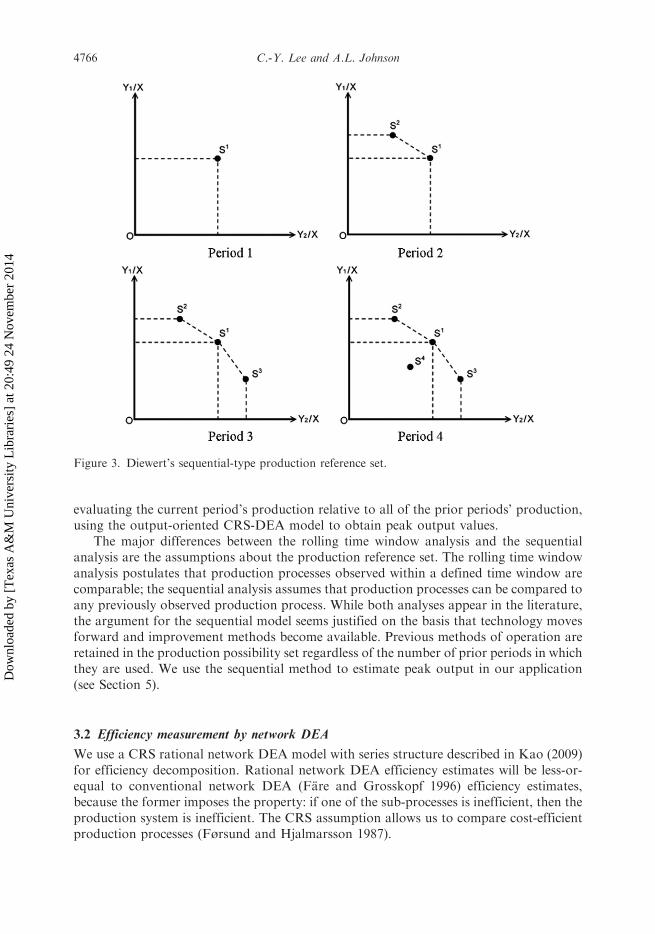
2. Production system decomposition
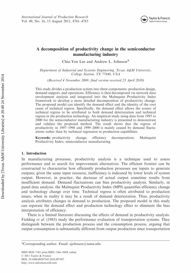
The production system comprises three phases, production design, demand support, andoperations, and this section will describe the system decomposition. A network DEAmodel is proposed to model the system; thus, the necessary linking variables are defined.Figure 1 shows the decomposition of the three phases.
The first phase, production design, defines the maximal output of the productionsystem with respect to capital investments. Inefficiency in this phase results from poorproduction design. The second phase describes demand support, where the sales grouptries to sell enough products to keep the facility at full operation. The inefficiency in thisphase results from insufficient demand, namely, production levels drop due to a lack of
Figure 1. System process decomposition.
International Journal of Production Research 4763
Dow
nloa
ded
by [
Tex
as A
&M
Uni
vers
ity L
ibra
ries
] at
20:
49 2
4 N
ovem
ber
2014
demand even though the production capacity is available. The third phase, operations,
transforms raw materials into final goods. The inefficiency of this phase results from the
poor integration of operational behaviour. In the semiconductor industry, the term ‘yield’
is usually employed in practice to describe the percentage of usable products resulting from
the production process. In contrast, the percentage of product lost, or ‘yield loss’, is the
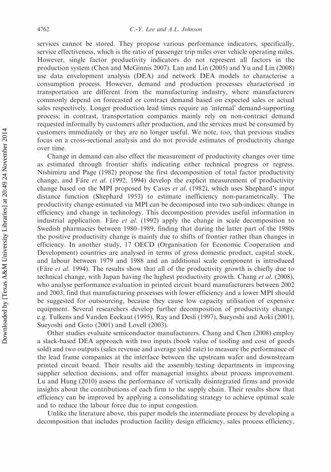
result of inefficiency of operations.This paper uses the following five metrics.
(1) Input resources are the items used to build up the infrastructure of the production
system and support the operations of the production process.(2) Peak output, the maximal output firms can achieve, characterises the ‘real
capability’ of the production system.(3) Demand is the quantity of product or output the customer is willing to consume at
the current industry price. In this study the demand is estimated by product start.
A product start is the release of raw materials to the production process. In the
semiconductor manufacturing industry, product starts (wafer starts) are used to
control the output level to match production and demand levels.(4) Actual output is the total of final products generated.
Input resource, product start, and actual output are typically collected directly from
the historical database, but peak output must be estimated (potential methods are
described in Section 3.1). Using the four metrics, the efficiency of the three sub-processes
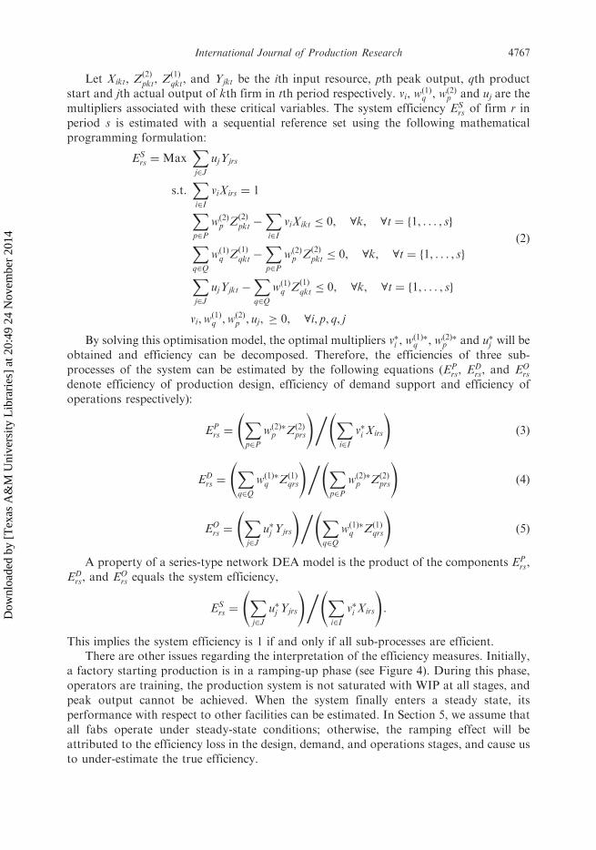
(production design, demand support, and operations) can be estimated respectively.Figure 2 illustrates the two possible scenarios that can occur between consumer and
producer:
(1) demand surplus occurs where the demand for a product exceeds the supply level, or
alternatively,(2) demand shortage occurs when the demand realised is less than the supply that can
be produced by the facility.
Figure 2. Scenarios of demand surplus and shortage.
4764 C.-Y. Lee and A.L. Johnson
Dow
nloa
ded
by [
Tex
as A
&M
Uni
vers
ity L
ibra
ries
] at
20:
49 2
4 N
ovem
ber
2014
In the first case, a firm may add more raw materials to the system. However, if the
system was previously operating optimally, the additional materials will lead to a higher
work-in-process (WIP) and increase the product cycle time (Hopp and Spearman 2001).
Thus, the production system would need to extend its operating hours or outsource the
additional demand. In the second case, a firm will attempt to match demand by controlling
the number of product starts1. We will focus on the second scenario, demand quantity is
less than peak output of the production system. However, demand shortage will be
underestimated for a firm that matches demand to actual output.
3. Measurement of efficiency decomposition
3.1 Peak output estimation
To apply the network DEA model suggested for production system decomposition, it is
necessary to quantify peak output. Two ways are suggested in the literature: a rolling time
window analysis (Charnes et al. 1985) and a sequential model (Diewert 1992).Rolling time window analysis estimates peak output via shifting time windows.
It postulates no technical change within any time window. Given a certain fixed number of
periods that define the time window, all observations of the production processes during
that window are compared in a single analysis (Charnes et al. 1985). Peak output is
estimated by using an output-oriented (CRS) DEA (Charnes et al. 1978), and a reference
set constructed from only the observations of the production process under analysis within
the time window. Let Xirt be the ith input resource of firm r in tth period, Zð1Þqrt the number
of product starts for the qth product of firm r in tth period, and �rt the multiplier of firm r
in tth period. �rs is the efficiency estimate of firm r in specific period s. The linear
programming formulation for a specific firm is:
Max �rs
s:t:Xt2TW
�rtXirt � Xirs, 8iXt2TW
�rtZð1Þqrt � �rsZ
ð1Þqrs, 8q
�rt � 0, 8t
ð1Þ
If efficiency equals 1, peak output equals the number of product starts in period s;
otherwise, the peak output is equal to product start multiplied by the efficiency estimate �rs.Then, the time window is shifted to include the next period, the oldest period in the time
window is dropped, and the process is repeated. Note that the reference set is
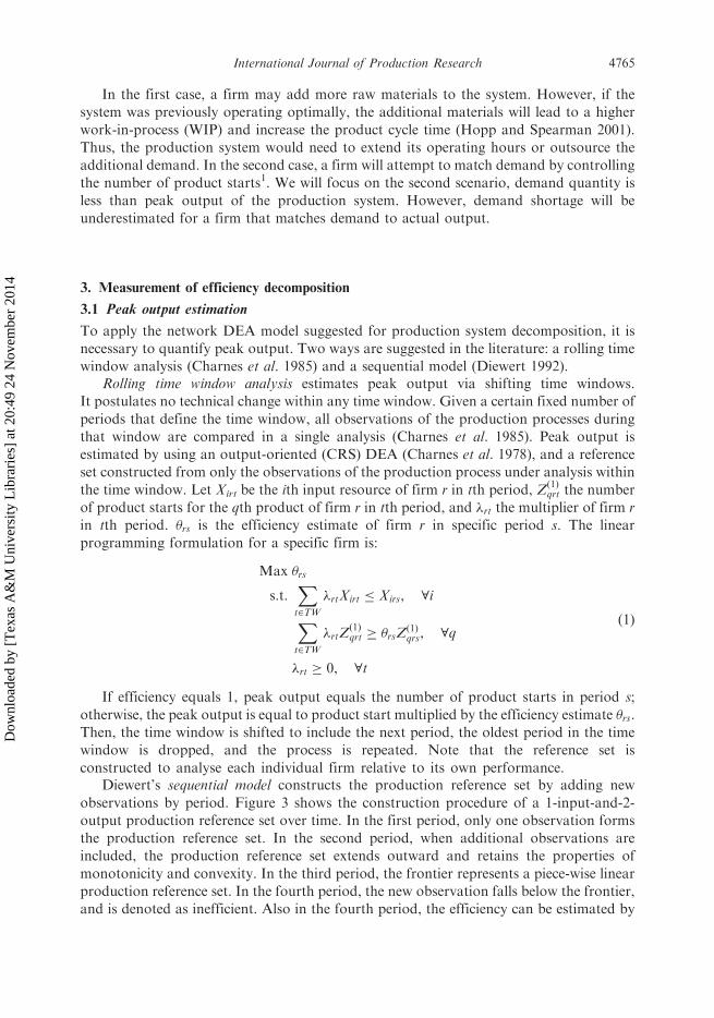
constructed to analyse each individual firm relative to its own performance.Diewert’s sequential model constructs the production reference set by adding new
observations by period. Figure 3 shows the construction procedure of a 1-input-and-2-
output production reference set over time. In the first period, only one observation forms
the production reference set. In the second period, when additional observations are
included, the production reference set extends outward and retains the properties of
monotonicity and convexity. In the third period, the frontier represents a piece-wise linear
production reference set. In the fourth period, the new observation falls below the frontier,
and is denoted as inefficient. Also in the fourth period, the efficiency can be estimated by
International Journal of Production Research 4765
Dow
nloa
ded
by [
Tex
as A
&M
Uni
vers
ity L
ibra
ries
] at
20:
49 2
4 N
ovem
ber
2014
evaluating the current period’s production relative to all of the prior periods’ production,using the output-oriented CRS-DEA model to obtain peak output values.
The major differences between the rolling time window analysis and the sequentialanalysis are the assumptions about the production reference set. The rolling time windowanalysis postulates that production processes observed within a defined time window arecomparable; the sequential analysis assumes that production processes can be compared toany previously observed production process. While both analyses appear in the literature,the argument for the sequential model seems justified on the basis that technology movesforward and improvement methods become available. Previous methods of operation areretained in the production possibility set regardless of the number of prior periods in whichthey are used. We use the sequential method to estimate peak output in our application(see Section 5).
3.2 Efficiency measurement by network DEA
We use a CRS rational network DEA model with series structure described in Kao (2009)for efficiency decomposition. Rational network DEA efficiency estimates will be less-or-equal to conventional network DEA (Fare and Grosskopf 1996) efficiency estimates,because the former imposes the property: if one of the sub-processes is inefficient, then theproduction system is inefficient. The CRS assumption allows us to compare cost-efficientproduction processes (Førsund and Hjalmarsson 1987).
Figure 3. Diewert’s sequential-type production reference set.
4766 C.-Y. Lee and A.L. Johnson
Dow
nloa
ded
by [
Tex
as A
&M
Uni
vers
ity L
ibra
ries
] at
20:
49 2
4 N
ovem
ber
2014
Let Xikt, Zð2Þpkt, Z
ð1Þqkt, and Yjkt be the ith input resource, pth peak output, qth product
start and jth actual output of kth firm in tth period respectively. vi, wð1Þq , wð2Þp and uj are the
multipliers associated with these critical variables. The system efficiency ESrs of firm r in
period s is estimated with a sequential reference set using the following mathematicalprogramming formulation:
ESrs ¼Max
Xj2J
ujYjrs
s:t:Xi2I
viXirs ¼ 1
Xp2P
wð2Þp Zð2Þpkt �
Xi2I
viXikt � 0, 8k, 8t ¼ f1, . . . , sg
Xq2Q
wð1Þq Zð1Þqkt �
Xp2P
wð2Þp Zð2Þpkt � 0, 8k, 8t ¼ f1, . . . , sg
Xj2J
ujYjkt �Xq2Q
wð1Þq Zð1Þqkt � 0, 8k, 8t ¼ f1, . . . , sg
vi,wð1Þq ,wð2Þp , uj, � 0, 8i, p, q, j
ð2Þ
By solving this optimisation model, the optimal multipliers v�i , wð1Þ�q , wð2Þ�p and u�j will be
obtained and efficiency can be decomposed. Therefore, the efficiencies of three sub-processes of the system can be estimated by the following equations (EP
rs, EDrs, and EO
rs
denote efficiency of production design, efficiency of demand support and efficiency ofoperations respectively):
EPrs ¼
Xp2P
wð2Þ�p Zð2Þprs
!� Xi2I
v�i Xirs
!ð3Þ
EDrs ¼
Xq2Q
wð1Þ�q Zð1Þqrs
!� Xp2P
wð2Þ�p Zð2Þprs
!ð4Þ
EOrs ¼
Xj2J
u�j Yjrs
!� Xq2Q
wð1Þ�q Zð1Þqrs
!ð5Þ
A property of a series-type network DEA model is the product of the components EPrs,
EDrs, and EO
rs equals the system efficiency,
ESrs ¼
Xj2J
u�j Yjrs
!� Xi2I
v�i Xirs
!:
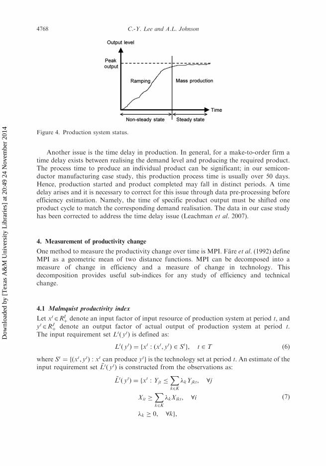
This implies the system efficiency is 1 if and only if all sub-processes are efficient.There are other issues regarding the interpretation of the efficiency measures. Initially,
a factory starting production is in a ramping-up phase (see Figure 4). During this phase,operators are training, the production system is not saturated with WIP at all stages, andpeak output cannot be achieved. When the system finally enters a steady state, its
performance with respect to other facilities can be estimated. In Section 5, we assume thatall fabs operate under steady-state conditions; otherwise, the ramping effect will beattributed to the efficiency loss in the design, demand, and operations stages, and cause usto under-estimate the true efficiency.
International Journal of Production Research 4767
Dow
nloa
ded
by [
Tex
as A
&M
Uni
vers
ity L
ibra
ries
] at
20:
49 2
4 N
ovem
ber
2014
Another issue is the time delay in production. In general, for a make-to-order firm atime delay exists between realising the demand level and producing the required product.The process time to produce an individual product can be significant; in our semicon-ductor manufacturing case study, this production process time is usually over 50 days.Hence, production started and product completed may fall in distinct periods. A timedelay arises and it is necessary to correct for this issue through data pre-processing beforeefficiency estimation. Namely, the time of specific product output must be shifted oneproduct cycle to match the corresponding demand realisation. The data in our case studyhas been corrected to address the time delay issue (Leachman et al. 2007).
4. Measurement of productivity change
One method to measure the productivity change over time is MPI. Fare et al. (1992) defineMPI as a geometric mean of two distance functions. MPI can be decomposed into ameasure of change in efficiency and a measure of change in technology. Thisdecomposition provides useful sub-indices for any study of efficiency and technicalchange.
4.1 Malmquist productivity index
Let xt2RIþ denote an input factor of input resource of production system at period t, and
yt2RJþ denote an output factor of actual output of production system at period t.
The input requirement set Ltð ytÞ is defined as:
Ltð ytÞ ¼ fxt : ðxt, ytÞ 2 Stg, t 2 T ð6Þ
where St ¼ fðxt, ytÞ : xt can produce ytg is the technology set at period t. An estimate of theinput requirement set ~Ltð ytÞ is constructed from the observations as:
~Ltð ytÞ ¼ fxt : Yjt �Xk2K
�kYjkt, 8j
Xit �Xk2K
�kXikt, 8i
�k � 0, 8kg,
ð7Þ
Figure 4. Production system status.
4768 C.-Y. Lee and A.L. Johnson
Dow
nloa
ded
by [
Tex
as A
&M
Uni
vers
ity L
ibra
ries
] at
20:
49 2
4 N
ovem
ber
2014
where �k indicate the intensity variables used in the piecewise linear technology. Note thatthe assumption of CRS is imposed on this reference technology set as suggested by Fareet al. (1994). For alternative assumptions, see for example Ray and Desli (1997). Then,defining Dt
Inputð yt, xtÞ as Shephard’s input-oriented distance function (Shephard 1953), the
efficiency of an observation at period t can be measured relative to the referencetechnology at period t:
DtInputð y
t, xtÞ ¼ supf� : ðxt=�Þ 2 Ltð ytÞg ð8Þ
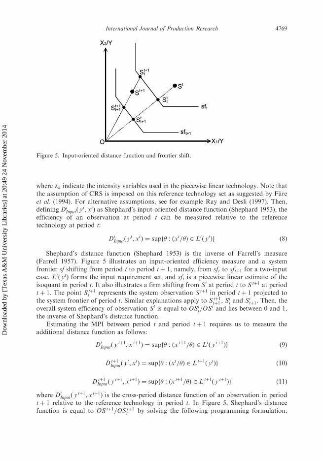
Shephard’s distance function (Shephard 1953) is the inverse of Farrell’s measure(Farrell 1957). Figure 5 illustrates an input-oriented efficiency measure and a systemfrontier sf shifting from period t to period tþ 1, namely, from sft to sftþ1 for a two-inputcase. Ltð ytÞ forms the input requirement set, and sft is a piecewise linear estimate of theisoquant in period t. It also illustrates a firm shifting from St at period t to Stþ1 at periodtþ 1. The point Stþ1
t represents the system observation Stþ1 in period tþ 1 projected tothe system frontier of period t. Similar explanations apply to Stþ1
tþ1 , Stt and St
tþ1. Then, theoverall system efficiency of observation St is equal to OSt
t=OSt and lies between 0 and 1,the inverse of Shephard’s distance function.
Estimating the MPI between period t and period tþ 1 requires us to measure theadditional distance function as follows:
DtInputð y
tþ1, x tþ1Þ ¼ supf� : ðxtþ1=�Þ 2 Ltð y tþ1Þg ð9Þ
Dtþ1Inputð y
t, xtÞ ¼ supf� : ðxt=�Þ 2 Ltþ1ð ytÞg ð10Þ
Dtþ1Inputð y
tþ1, xtþ1Þ ¼ supf� : ðx tþ1=�Þ 2 Ltþ1ð y tþ1Þg ð11Þ
where DtInputð y
tþ1, xtþ1Þ is the cross-period distance function of an observation in periodtþ 1 relative to the reference technology in period t. In Figure 5, Shephard’s distancefunction is equal to OStþ1=OStþ1
t by solving the following programming formulation.
Figure 5. Input-oriented distance function and frontier shift.
International Journal of Production Research 4769
Dow
nloa
ded
by [
Tex
as A
&M
Uni
vers
ity L
ibra
ries
] at
20:
49 2
4 N
ovem
ber
2014
Similarly, Dtþ1Inputð y
t, xtÞ and Dtþ1Inputð y
tþ1, x tþ1Þ can be defined:
½DtInputð y
tþ1, x tþ1Þ��1¼Min �
s:t: Yjrðtþ1Þ �Xk2K
�kYjkt, 8j
�Xirðtþ1Þ �Xk2K
�kXikt, 8i
�k � 0, 8k
ð12Þ
Fare et al. (1992, 1994) propose an input-oriented MPI at period t relative toperiod tþ 1 as:
MPItþ1�4tInput ð y
tþ1,x tþ1, yt,xtÞ ¼Dt
Inputð ytþ1, x tþ1Þ
DtInputð y
t, xtÞ
Dtþ1Inputð y
tþ1, x tþ1Þ
Dtþ1Inputð y
t, xtÞ
" #12
ð13Þ
and this index can be decomposed into change in efficiency (CIE) and change intechnology (CIT) at period tþ 1 relative to period t as:
MPIt�4tþ1Input ð y
tþ1, xtþ1, yt, xtÞ ¼Dt
Inputð yt, xtÞ
Dtþ1Inputð y
tþ1, xtþ1Þ
Dtþ1Inputð y
tþ1, xtþ1Þ
DtInputð y
tþ1, xtþ1Þ
Dtþ1Inputð y
t, xtÞ
DtInputð y
t, xtÞ
" #12
ð14Þ
where the first term represents the change in efficiency from period t to period tþ 1, andthe second term indicates the change in technology. Let TSEt ¼ 1=Dt
Inputð yt,xtÞ
and TSEtþ1 ¼ 1=Dtþ1Inputð y
tþ1, x tþ1Þ as technical and scale efficiency (TSE) at period t
and tþ 1, and IEI tþ1t ¼ 1=DtInputð y
tþ1, x tþ1Þ and IEIttþ1 ¼ 1=Dtþ1Inputð y
t,xtÞ as intertemporalefficiency index (IEI) at period tþ 1 relative to the reference technology at period t, and atperiod t relative to the reference technology at period tþ 1. Therefore, based on input-oriented measurement, the change in productivity, change in efficiency, and change intechnology are each interpreted as achieving progress, no change, and regress when thevalues for their estimates are greater than 1, equal to 1, and less than 1.
4.2 Efficiency decomposition of MPI
The decomposition of efficiency proposed in Section 3.2 defines system efficiency ES asequal to the product of production design efficiency EP, demand support efficiency ED,and operations efficiency EO, ES ¼ EP � ED � EO. Thus, we show that the MPI of theoverall production system (SMPI) equals the MPI multiplication of production design(PMPI), demand support (DMPI), and operations (OMPI), namely,
SMPI tþ1t ¼ PMPItþ1t �DMPItþ1t �OMPItþ1t : ð15Þ
Below, the necessary notation and definitions are outlined to show (15) must hold.First we demonstrate that equation SMPItþ1t ¼ PMPI tþ1t �DOMPItþ1t holds, and thenwe show DOMPI tþ1t ¼ DMPItþ1t �OMPItþ1t .
The efficiencies of demand support and operations are combined in one compositeefficiency EDO; thus, system efficiency is ES ¼ EP � EDO. Since all of the distance functionsused in the following sections are input-oriented measurements, we drop the subscript inputfor notational simplicity. Let St and Pt be the observations of overall production system
4770 C.-Y. Lee and A.L. Johnson
Dow
nloa
ded
by [
Tex
as A
&M
Uni
vers
ity L
ibra
ries
] at
20:
49 2
4 N
ovem
ber
2014
and production design, and sft and pft be the efficiency frontier of overall production system
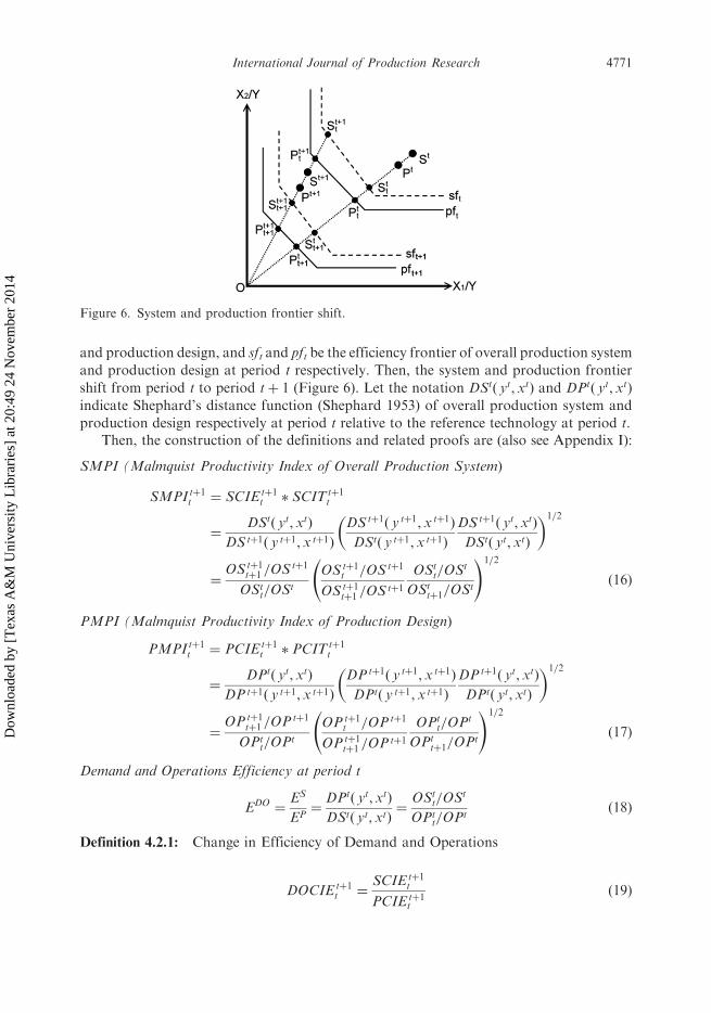
and production design at period t respectively. Then, the system and production frontier
shift from period t to period tþ 1 (Figure 6). Let the notation DStð yt, xtÞ and DPtð yt, xtÞ
indicate Shephard’s distance function (Shephard 1953) of overall production system and
production design respectively at period t relative to the reference technology at period t.Then, the construction of the definitions and related proofs are (also see Appendix I):
SMPI (Malmquist Productivity Index of Overall Production System)
SMPItþ1t ¼ SCIEtþ1t � SCITtþ1
t
¼DStð yt, xtÞ
DStþ1ð y tþ1, xtþ1Þ
DStþ1ð y tþ1, x tþ1Þ
DStð y tþ1, xtþ1Þ
DStþ1ð yt, xtÞ
DStð yt, xtÞ
� �1=2
¼OStþ1
tþ1 =OStþ1
OStt=OSt
OStþ1t =OStþ1
OStþ1tþ1 =OStþ1
OStt=OSt
OSttþ1=OSt
!1=2
ð16Þ
PMPI (Malmquist Productivity Index of Production Design)
PMPItþ1t ¼ PCIEtþ1t � PCITtþ1
t
¼DPtð yt, xtÞ
DPtþ1ð y tþ1, xtþ1Þ
DPtþ1ð y tþ1, x tþ1Þ
DPtð y tþ1, xtþ1Þ
DPtþ1ð yt, xtÞ
DPtð yt, xtÞ
� �1=2
¼OPtþ1
tþ1 =OPtþ1
OPtt=OPt
OPtþ1t =OPtþ1
OPtþ1tþ1 =OPtþ1
OPtt=OPt
OPttþ1=OPt
!1=2
ð17Þ
Demand and Operations Efficiency at period t
EDO ¼ES
EP¼
DPtð yt,xtÞ
DStð yt, xtÞ¼
OStt=OSt
OPtt=OPt
ð18Þ
Definition 4.2.1: Change in Efficiency of Demand and Operations
DOCIEtþ1t ¼
SCIEtþ1t
PCIEtþ1t
ð19Þ
Figure 6. System and production frontier shift.
International Journal of Production Research 4771
Dow
nloa
ded
by [
Tex
as A
&M
Uni
vers
ity L
ibra
ries
] at
20:
49 2
4 N
ovem
ber
2014
Definition 4.2.2: Change in Technology of Demand and Operations
DOCITtþ1t ¼
SCITtþ1t
PCITtþ1t
ð20Þ
Definition 4.2.3: Malmquist Productivity Index of Demand and Operations
DOMPItþ1t ¼SMPItþ1t
PMPI tþ1t
ð21Þ
Based on the definitions, the equation SMPI tþ1t ¼ PMPItþ1t �DOMPItþ1t is deriveddirectly. Through a similar procedure, it can be shown that DOMPItþ1t ¼
DMPItþ1t �OMPItþ1t , where DMPItþ1t and OMPItþ1t are the MPI of demand supportand operations respectively. Thus, the efficiency decomposition of the MPI of the overallproduction system is SMPI tþ1t ¼ PMPItþ1t �DMPItþ1t �OMPItþ1t .
5. Empirical study
This section will analyse the semiconductor manufacturing industry. The data set isdescribed in Leachman et al. (2007). The data includes 87 records collected from 10 leadingfabs which produced 200mm wafers with 350 nm process technology in the United States,Taiwan, Japan, and Europe from 1995 to 2000. Each observation is a particular fab in agiven quarter of a specific year. The data definitions of input-output factors forproductivity analysis are described in Section 5.1. In Section 5.2, employing thedecomposition of efficiency and applying the MPI to quantify productivity changeallows a more detailed analysis of the source of inefficiency within each fab. Section 5.3shows the efficiency difference between logic and memory products using two-stage DEA.
5.1 Data description
The production process in semiconductor manufacturing can be characterised by thefollowing input resources:
. Number of steppers (SN) is the average number of steppers and scanners employedin the fab during a particular quarter. Steppers and scanners are exposure toolsused in the lithography process to define the pattern of integrated circuit andcritical dimension by depositing layers and doping region. In practice, thelithography process is typically the bottleneck of the production line, because it isthe most expensive machinery in the facility.
. Headcount (HC) is the sum of direct and indirect headcount. Direct headcountrefers to the operators and workers who operate machinery used in theproduction process; indirect headcount refers to the engineers, technicians andmanagers who support the related business activities. The amount of indirectlabour is relatively stable regardless of variation in the production volume.
. Clean-room size (CR) indicates the size of the floor space in a clean room. A cleanroom controls particle dispersion and creates an uncontaminated condition formanufacturing. A general rule of thumb is that a fab’s infrastructure (capital)costs are proportional to its CR. In other words, CR is a proxy for the totalinvestment in a fab’s infrastructure. The data for CR is the sum of depreciatedconstruction cost and occupation cost per square foot during a quarter.
4772 C.-Y. Lee and A.L. Johnson
Dow
nloa
ded
by [
Tex
as A
&M
Uni
vers
ity L
ibra
ries
] at
20:
49 2
4 N
ovem
ber
2014
. Total wafer starts (WS) is the total number of blank silicon wafers released intothe manufacturing process during a particular quarter. Wafer starts mainlydepend on production capacity and demand requirements. Too many wafer startswill create high levels of WIP and extend cycle times; insufficient wafer startscause loss of capacity and lower machine utilisation. In general, WS controls thelevel of production output based on demand information.
. Actual die output (AD) represents the amount of saleable die output actuallyproduced by the fabrication process during a particular quarter.
. Peak die output (PD) is the highest output level under a given production design.This unobservable variable can be estimated via a sequential model whichassumes that past performance can be used as a reference set for estimating WS.
Other factors which also affect fab operations and productivity, but which are notinputs or outputs to the production process, are often referred to as contextual variables inthe productivity literature. Examples are: product mix, employment of automated materialhandling system (AMHS) and equipment type. In the application below the decompositionof efficiency is extended to consider the effects of product type on the productivity of a fabusing a two-stage approach (Ray 1988, 1991). Product types influence fab resourceallocation, and require dedicated equipment and specific changeover procedures. Differentproduct types may have different numbers of mask layers which increase productcomplexity, and lead to a significant difference of efficiencies. The effects of other practicesor attributes can also be analysed using this same approach.
5.2 Productivity change analysis
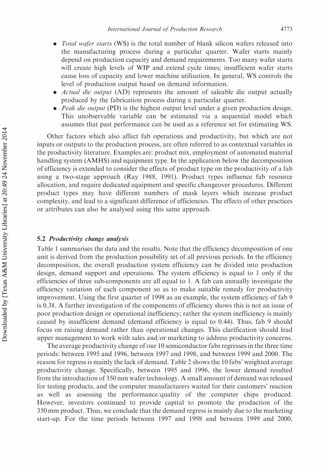
Table 1 summarises the data and the results. Note that the efficiency decomposition of oneunit is derived from the production possibility set of all previous periods. In the efficiencydecomposition, the overall production system efficiency can be divided into productiondesign, demand support and operations. The system efficiency is equal to 1 only if theefficiencies of three sub-components are all equal to 1. A fab can annually investigate theefficiency variation of each component so as to make suitable remedy for productivityimprovement. Using the first quarter of 1998 as an example, the system efficiency of fab 9is 0.38. A further investigation of the components of efficiency shows this is not an issue ofpoor production design or operational inefficiency; rather the system inefficiency is mainlycaused by insufficient demand (demand efficiency is equal to 0.44). Thus, fab 9 shouldfocus on raising demand rather than operational changes. This clarification should leadupper management to work with sales and/or marketing to address productivity concerns.
The average productivity change of our 10 semiconductor fabs regresses in the three timeperiods: between 1995 and 1996, between 1997 and 1998, and between 1999 and 2000. Thereason for regress is mainly the lack of demand. Table 2 shows the 10 fabs’ weighted averageproductivity change. Specifically, between 1995 and 1996, the lower demand resultedfrom the introduction of 350mmwafer technology. A small amount of demandwas releasedfor testing products, and the computer manufacturers waited for their customers’ reactionas well as assessing the performance/quality of the computer chips produced.However, investors continued to provide capital to promote the production of the350mm product. Thus, we conclude that the demand regress is mainly due to the marketingstart-up. For the time periods between 1997 and 1998 and between 1999 and 2000,
International Journal of Production Research 4773
Dow
nloa
ded
by [
Tex
as A
&M
Uni
vers
ity L
ibra
ries
] at
20:
49 2
4 N
ovem
ber
2014
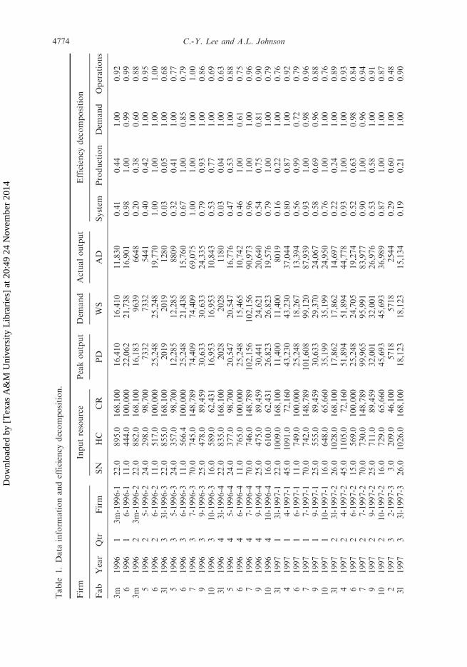
Table
1.Data
inform
ationandefficiency
decomposition.
Firm
Inputresource
Peakoutput
Dem
and
Actualoutput
Efficiency
decomposition
Fab
Year
Qtr
Firm
SN
HC
CR
PD
WS
AD
System
Production
Dem
and
Operations
3m
1996
13m-1996-1
22.0
895.0
168,100
16,410
16,410
11,830
0.41
0.44
1.00
0.92
61996
16-1996-1
11.0
444.0
100,000
22,062
21,738
16,901
0.98
1.00
0.99
0.99
3m
1996
23m-1996-2
22.0
882.0
168,100
16,183
9639
6648
0.20
0.38
0.60
0.88
51996
25-1996-2
24.0
298.0
98,700
7332
7332
5441
0.40
0.42
1.00
0.95
61996
26-1996-2
11.0
517.0
100,000
25,248
25,248
19,770
1.00
1.00
1.00
1.00
3l
1996
33l-1996-3
22.0
855.0
168,100
2019
2019
1280
0.03
0.05
1.00
0.68
51996
35-1996-3
24.0
357.0
98,700
12,285
12,285
8809
0.32
0.41
1.00
0.77
61996
36-1996-3
11.0
566.4
100,000
25,248
21,438
15,760
0.67
1.00
0.85
0.79
71996
37-1996-3
70.0
745.0
148,789
74,409
74,409
69,075
1.00
1.00
1.00
1.00
91996
39-1996-3
25.0
478.0
89,459
30,633
30,633
24,335
0.79
0.93
1.00
0.86
10
1996
310-1996-3
16.0
589.0
62,431
16,953
16,953
10,843
0.53
0.77
1.00
0.69
3l
1996
43l-1996-4
22.0
835.0
168,100
2028
2028
1180
0.03
0.04
1.00
0.63
51996
45-1996-4
24.0
377.0
98,700
20,547
20,547
16,776
0.47
0.53
1.00
0.88
61996
46-1996-4
11.0
765.0
100,000
25,248
15,465
10,742
0.46
1.00
0.61
0.75
71996
47-1996-4
70.0
746.0
148,789
102,156
102,156
90,973
0.96
1.00
1.00
0.96
91996
49-1996-4
25.0
475.0
89,459
30,441
24,621
20,640
0.54
0.75
0.81
0.90
10
1996
410-1996-4
16.0
610.0
62,431
26,823
26,823
19,576
0.79
1.00
1.00
0.79
3l
1997
13l-1997-1
22.0
1009.0
168,100
11,400
11,400
8019
0.16
0.22
1.00
0.76
41997
14-1997-1
45.0
1091.0
72,160
43,230
43,230
37,044
0.80
0.87
1.00
0.92
61997
16-1997-1
11.0
749.0
100,000
25,248
18,267
13,394
0.56
0.99
0.72
0.79
71997
17-1997-1
70.0
742.0
148,789
101,608
99,120
87,939
0.93
1.00
0.98
0.96
91997
19-1997-1
25.0
555.0
89,459
30,633
29,370
24,067
0.58
0.69
0.96
0.88
10
1997
110-1997-1
16.0
648.0
65,660
35,199
35,199
24,950
0.76
1.00
1.00
0.76
3l
1997
23l-1997-2
26.0
1028.0
168,100
17,862
17,862
14,697
0.22
0.24
1.00
0.89
41997
24-1997-2
45.0
1105.0
72,160
51,894
51,894
44,778
0.93
1.00
1.00
0.93
61997
26-1997-2
15.0
569.0
100,000
25,248
24,705
19,274
0.52
0.63
0.98
0.84
71997
27-1997-2
70.0
730.0
148,789
99,965
95,991
83,977
0.90
1.00
0.96
0.94
91997
29-1997-2
25.0
711.0
89,459
32,001
32,001
26,976
0.53
0.58
1.00
0.91
10
1997
210-1997-2
16.0
729.0
65,660
45,693
45,693
36,989
0.87
1.00
1.00
0.87
21997
32-1997-3
3.0
209.0
46,100
5718
5718
2544
0.29
0.60
1.00
0.48
3l
1997
33l-1997-3
26.0
1026.0
168,100
18,123
18,123
15,134
0.19
0.21
1.00
0.90
4774 C.-Y. Lee and A.L. Johnson
Dow
nloa
ded
by [
Tex
as A
&M
Uni
vers
ity L
ibra
ries
] at
20:
49 2
4 N
ovem
ber
2014
61997
36-1997-3
15.0
581.0
100,000
25,248
24,564
20,374
0.46
0.53
0.97
0.89
71997
37-1997-3
70.0
712.0
148,789
97,500
92,193
79,019
0.87
0.99
0.95
0.92
91997
39-1997-3
25.7
750.0
89,459
78,258
78,258
63,251
0.87
1.00
1.00
0.87
10
1997
310-1997-3
16.0
849.0
65,660
45,693
40,131
32,341
0.71
0.93
0.88
0.87
21997
42-1997-4
3.3
224.0
46,100
9840
9840
6340
0.55
0.80
1.00
0.69
3l
1997
43l-1997-4
26.0
1133.0
168,100
18,123
17,811
15,516
0.16
0.18
0.98
0.94
61997
46-1997-4
15.0
608.0
100,000
25,248
22,833
19,525
0.37
0.44
0.90
0.92
71997
47-1997-4
70.0
688.0
148,789
94,214
86,253
73,765
0.83
0.99
0.92
0.92
91997
49-1997-4
27.0
783.0
89,459
97,575
97,575
78,319
0.86
1.00
1.00
0.86
10
1997
410-1997-4
16.0
973.0
65,660
45,693
42,732
31,950
0.59
0.78
0.94
0.81
21998
12-1998-1
4.8
216.0
46,100
9489
8886
5257
0.30
0.51
0.94
0.64
61998
16-1998-1
17.0
651.0
100,000
29,742
29,742
23,222
0.38
0.45
1.00
0.84
71998
17-1998-1
73.0
658.0
148,789
90,105
87,918
79,924
0.94
0.98
0.98
0.98
81998
18-1998-1
28.0
1022.0
80,735
4911
4911
3931
0.05
0.06
1.00
0.86
91998
19-1998-1
27.0
798.0
89,459
97,575
42,786
34,454
0.38
1.00
0.44
0.87
10
1998
110-1998-1
16.0
1072.0
65,660
63,423
63,423
45,455
0.77
1.00
1.00
0.77
21998
22-1998-2
6.0
258.0
46,100
12,750
12,750
6737
0.32
0.55
1.00
0.57
61998
26-1998-2
17.0
899.0
100,000
29,742
13,212
10,983
0.18
0.44
0.44
0.90
71998
27-1998-2
75.0
658.0
148,789
90,579
90,579
83,841
0.98
0.99
1.00
1.00
81998
28-1998-2
28.0
1165.0
80,735
6294
6294
4980
0.06
0.07
1.00
0.85
11998
31-1998-3
35.0
1230.0
100,000
24,168
24,168
17,201
0.17
0.22
1.00
0.76
21998
32-1998-3
6.8
400.0
46,100
16,359
16,359
10,526
0.42
0.61
1.00
0.69
61998
36-1998-3
17.0
888.0
100,000
29,742
6042
5090
0.08
0.44
0.20
0.90
71998
37-1998-3
75.0
560.0
148,789
88,710
88,710
82,605
1.00
1.00
1.00
1.00
81998
38-1998-3
28.0
1160.0
80,735
6762
6762
5061
0.06
0.08
1.00
0.80
11998
41-1998-4
35.0
1244.0
100,000
35,601
35,601
25,870
0.25
0.33
1.00
0.78
21998
42-1998-4
7.5
287.0
46,100
13,487
9276
6100
0.23
0.48
0.69
0.71
61998
46-1998-4
17.0
752.0
100,000
29,742
14,550
12,659
0.20
0.45
0.49
0.93
81998
48-1998-4
28.0
1161.0
80,735
14,103
14,103
10,145
0.12
0.16
1.00
0.77
11999
11-1999-1
35.0
1289.0
100,000
41,457
41,457
31,538
0.31
0.38
1.00
0.82
21999
12-1999-1
8.0
375.0
46,100
17,031
17,031
11,748
0.41
0.55
1.00
0.74
81999
18-1999-1
28.0
1177.0
80,735
29,445
29,445
19,826
0.24
0.33
1.00
0.72
11999
21-1999-2
35.0
1337.0
100,000
41,988
41,988
32,881
0.32
0.38
1.00
0.84
21999
22-1999-2
8.0
373.0
46,100
17,043
17,043
11,799
0.41
0.55
1.00
0.74
81999
28-1999-2
28.0
1304.0
80,735
34,620
34,620
22,520
0.27
0.39
1.00
0.70
11999
31-1999-3
35.0
1322.0
100,000
41,822
40,071
31,550
0.31
0.38
0.96
0.85
(continued
)
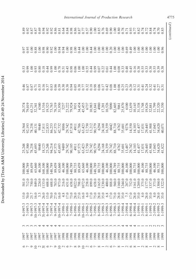
International Journal of Production Research 4775
Dow
nloa
ded
by [
Tex
as A
&M
Uni
vers
ity L
ibra
ries
] at
20:
49 2
4 N
ovem
ber
2014
Table
1.Continued.
Firm
Inputresource
Peakoutput
Dem
and
Actualoutput
Efficiency
decomposition
Fab
Year
Qtr
Firm
SN
HC
CR
PD
WS
AD
System
Production
Dem
and
Operations
21999
32-1999-3
8.0
391.0
46,100
20,517
20,517
13,342
0.46
0.66
1.00
0.70
81999
38-1999-3
28.0
1360.0
80,735
42,024
42,024
29,182
0.36
0.48
1.00
0.75
11999
41-1999-4
35.0
1292.0
100,000
41,490
27,312
22,550
0.22
0.38
0.66
0.89
21999
42-1999-4
9.3
437.0
46,100
20,517
15,177
9194
0.28
0.58
0.74
0.65
81999
48-1999-4
29.2
1471.0
80,735
42,024
38,058
26,354
0.32
0.48
0.91
0.74
12000
11-2000-1
35.0
1276.0
100,000
41,039
19,851
15,897
0.16
0.38
0.48
0.86
22000
12-2000-1
10.0
465.0
46,100
20,517
17,049
10,397
0.29
0.54
0.83
0.65
82000
18-2000-1
31.0
1545.0
80,735
42,024
32,127
21,768
0.27
0.48
0.76
0.73
12000
21-2000-2
35.0
1280.0
100,000
41,168
15,756
13,035
0.13
0.38
0.38
0.89
22000
22-2000-2
10.0
514.0
46,100
20,517
4734
2947
0.08
0.53
0.23
0.67
82000
28-2000-2
31.0
1722.0
80,735
42,024
30,255
18,422
0.22
0.48
0.72
0.65
12000
31-2000-3
35.0
1272.0
100,000
40,910
10,290
8,497
0.08
0.37
0.25
0.89
82000
38-2000-3
31.0
1881.0
80,735
44,415
44,415
26,036
0.32
0.50
1.00
0.63
4776 C.-Y. Lee and A.L. Johnson
Dow
nloa
ded
by [
Tex
as A
&M
Uni
vers
ity L
ibra
ries
] at
20:
49 2
4 N
ovem
ber
2014
Table
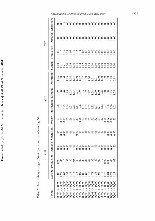
2.Productivitychangeofsemiconductormanufacturingfabs.
Period
MPI
CIE
CIT
System
Production
Dem
and
Operations
System
Production
Dem
and
Operations
System
Production
Dem
and
Operations
4Q95–4
1Q96
1.02
0.98
0.99
1.05
1.02
0.98
0.99
1.06
1.00
1.00
1.00
1.00
1Q96–4
2Q96
0.99
1.06
0.90
0.99
0.89
0.95
0.90
0.98
1.11
1.12
1.00
1.00
2Q96–4
3Q96
1.03
1.16
0.90
0.95
0.72
0.99
0.90
0.80
1.41
1.18
1.00
1.19
3Q96–4
4Q96
1.33
1.32
0.95
1.01
1.02
1.04
0.95
1.03
1.30
1.27
1.00
1.00
4Q96–4
1Q97
1.35
1.30
1.03
1.01
1.26
1.21
1.03
1.04
1.06
1.07
1.00
1.00
1Q97–4
2Q97
1.16
1.08
1.03
1.04
1.04
0.98
1.03
1.07
1.10
1.11
1.00
1.00
2Q97–4
3Q97
1.35
1.40
0.97
0.99
1.13
1.17
0.97
1.00
1.15
1.15
1.00
1.00
3Q97–4
4Q97
1.09
1.09
0.99
1.00
0.96
0.96
0.99
1.07
1.14
1.14
1.00
1.00
4Q97–4
1Q98
1.05
1.08
0.95
1.00
1.02
1.05
0.95
0.97
1.02
1.02
1.00
1.00
1Q98–4
2Q98
1.00
1.02
0.97
1.01
1.00
1.02
0.97
0.99
1.00
1.00
1.00
1.00
2Q98–4
3Q98
1.10
1.08
0.97
1.03
1.02
1.02
0.97
1.04
1.08
1.06
1.00
1.00
3Q98–4
4Q98
1.73
1.32
1.24
1.01
1.73
1.32
1.24
1.01
1.00
1.00
1.00
1.00
4Q98–4
1Q99
1.55
1.47
1.09
1.01
1.55
1.47
1.09
1.01
1.00
1.00
1.00
1.00
1Q99–4
2Q99
1.07
1.07
1.00
1.00
1.07
1.07
1.00
1.00
1.00
1.00
1.00
1.00
2Q99–4
3Q99
1.12
1.12
0.98
1.02
1.12
1.12
0.98
1.00
1.00
1.00
1.00
1.00
3Q99–4
4Q99
0.78
0.97
0.80
1.01
0.78
0.97
0.80
0.99
1.00
1.00
1.00
1.00
4Q99–4
1Q00
0.84
0.98
0.88
0.98
0.84
0.98
0.88
0.99
1.00
1.00
1.00
1.00
1Q00–4
2Q00
0.79
1.00
0.83
0.96
0.79
1.00
0.83
0.98
1.00
1.00
1.00
1.00
2Q00–4
3Q00
1.23
1.03
1.25
0.97
1.23
1.03
1.25
0.98
1.00
1.00
1.00
1.00
International Journal of Production Research 4777
Dow
nloa
ded
by [
Tex
as A
&M
Uni
vers
ity L
ibra
ries
] at
20:
49 2
4 N
ovem
ber
2014
the technology process matured and capacity growth was stable. Thus, we conclude thedemand regress is mainly due to demand fluctuation.
For the first and second quarters of 1996, the MPI of the overall system is 0.99.The production design component is 1.06, the demand support component is 0.90 and theoperational component is 0.99. Considering each component individually, a 6%improvement on average of design efficiency over the time horizon is observed, indicatingthe fabs have been proactive in improving their design process. Demand efficiency equal to0.90 indicates that some fabs are failing to generate demand sufficient to keep theproduction facility operating efficiently. Some excess capacity is expected due to randomdemand fluctuations; however, there still seems to be significant room for improvement.Finally, operations efficiency equal to 0.99 indicates that most fabs are operatingefficiently. Therefore, they should promote their devices and stimulate demand as the mosteffective way to improve productivity.2
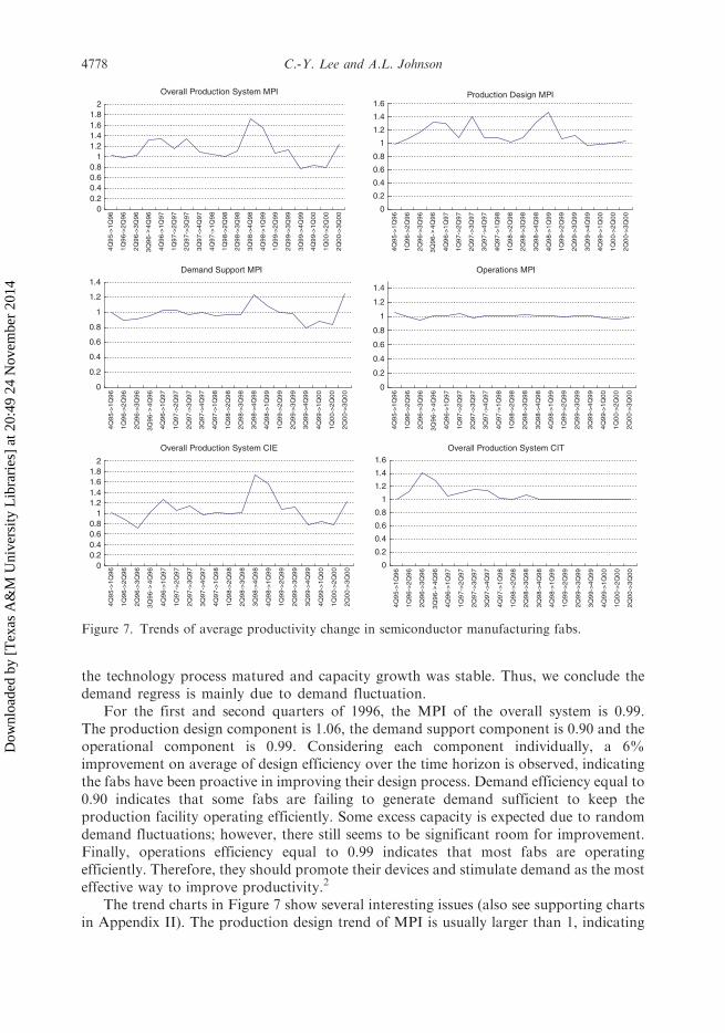
The trend charts in Figure 7 show several interesting issues (also see supporting chartsin Appendix II). The production design trend of MPI is usually larger than 1, indicating
Overall Production System MPI
00.20.40.60.8
11.21.41.61.8
24
Q9
5->
1Q96
1Q
96-
>2Q
96
2Q
96-
>3Q
96
3Q
96-
4Q
96
4Q
96-
>1Q
97
1Q
97-
>2Q
97
2Q
97-
>3Q
97
3Q
97-
>4Q
97
4Q
97-
>1Q
98
1Q
98-
>2Q
98
2Q
98-
>3Q
98
3Q
98-
>4Q
98
4Q
98-
>1Q
99
1Q
99-
>2Q
99
2Q
99-
>3Q
99
3Q
99-
>4Q
99
4Q
99-
>1Q
00
1Q
00-
>2Q
00
2Q
00-
>3Q
00
Production Design MPI
0
0.2
0.4
0.6
0.8
1
1.2
1.4
1.6
4Q
95-
>1Q
96
1Q
96-
>2Q
96
2Q
96-
>3Q
96
3Q
96-
4Q96
4Q
96-
>1Q
97
1Q
97-
>2Q
97
2Q
97-
>3Q
97
3Q
97-
>4Q
97
4Q
97-
>1Q
98
1Q
98-
>2Q
98
2Q
98-
>3Q
98
3Q
98-
>4Q
98
4Q
98-
>1Q
99
1Q
99-
>2Q
99
2Q
99-
>3Q
99
3Q
99-
>4Q
99
4Q
99-
>1Q
00
1Q
00-
>2Q
00
2Q
00-
>3Q
00
Demand Support MPI
0
0.2
0.4
0.6
0.8
1
1.2
1.4
4Q
95-
>1Q
96
1Q
96-
>2Q
96
2Q
96-
>3Q
96
3Q
96 -
4Q96
4Q
96-
>1Q
97
1Q
97-
>2Q
97
2Q
97-
>3Q
97
3Q
97-
>4Q
97
4Q
97-
>1Q
98
1Q
98-
>2Q
98
2Q
98-
>3Q
98
3Q
98-
>4Q
98
4Q
98-
>1Q
99
1Q
99-
>2Q
99
2Q
99-
>3Q
99
3Q
99-
>4Q
99
4Q
99-
>1Q
00
1Q
00-
>2Q
00
2Q
00-
>3Q
00
Operations MPI
0
0.2
0.4
0.6
0.8
1
1.2
1.4
4Q
95-
>1Q
96
1Q
96-
>2Q
96
2Q
96-
>3Q
96
3Q
96-
4Q96
4Q
96-
>1Q
97
1Q
97-
>2Q
97
2Q
97-
>3Q
97
3Q
97-
>4Q
97
4Q
97-
>1Q
98
1Q
98-
>2Q
98
2Q
98-
>3Q
98
3Q
98-
>4Q
98
4Q
98-
>1Q
99
1Q
99-
>2Q
99
2Q
99-
>3Q
99
3Q
99-
>4Q
99
4Q
99-
>1Q
00
1Q
00-
>2Q
00
2Q
00-
>3Q
00
Overall Production System CIE
00.20.40.60.8
11.21.41.61.8
2
4Q
95-
>1Q
96
1Q
96-
>2Q
96
2Q
96-
>3Q
96
3Q
96-
4Q96
4Q
96-
>1Q
97
1Q
97-
>2Q
97
2Q
97-
>3Q
97
3Q
97-
>4Q
97
4Q
97-
>1Q
98
1Q
98-
>2Q
98
2Q
98-
>3Q
98
3Q
98-
>4Q
98
4Q
98-
>1Q
99
1Q
99-
>2Q
99
2Q
99-
>3Q
99
3Q
99-
>4Q
99
4Q
99-
>1Q
00
1Q
00-
>2Q
00
2Q
00-
>3Q
00
Overall Production System CIT
0
0.2
0.4
0.6
0.8
1
1.2
1.4
1.6
4Q
95-
>1Q
96
1Q
96-
>2Q
96
2Q
96-
>3Q
96
3Q
96-
4Q96
4Q
96-
>1Q
97
1Q
97-
>2Q
97
2Q
97-
>3Q
97
3Q
97-
>4Q
97
4Q
97-
>1Q
98
1Q
98-
>2Q
98
2Q
98-
>3Q
98
3Q
98-
>4Q
98
4Q
98-
>1Q
99
1Q
99-
>2Q
99
2Q
99-
>3Q
99
3Q
99-
>4Q
99
4Q
99-
>1Q
00
1Q
00-
>2Q
00
2Q
00-
>3Q
00Figure 7. Trends of average productivity change in semiconductor manufacturing fabs.
4778 C.-Y. Lee and A.L. Johnson
Dow
nloa
ded
by [
Tex
as A
&M
Uni
vers
ity L
ibra
ries
] at
20:
49 2
4 N
ovem
ber
2014

that the fabs are consistently improving by upgrading existing processes and equipment.The demand trend of the MPI fluctuates above and below 1, which indicates demand inthe semiconductor manufacturing industry is tied to prosperity cycles. In fact, demanddeteriorated from 1997 to 1998 and from 1999 to 2000; note that the second quarter isusually the weakest demand quarter. Operations productivity index is usually close to 1with small variation, which indicates that fabs consistently perform operational processeswell. In addition, the trend of the production design component is similar to that of theoverall production system, and the variation of the production design component is largerthan the other two components. Both indicate that the production design process is asignificant sub-process and will lead to a long-term effect on productivity. The demandsub-process has a minor effect. The MPI of the overall system follows a similar pattern ofCIE, but CIT tends to converge to 1, because CIE has a larger variation than CIT.For instance, a deteriorated CIE from 1999 to 2000 is mainly caused by insufficientdemand; however, CIT would not represent a regress of the production frontier, since asequential model is employed for efficiency estimation; CIT is never less than 1.
Productivity change analysis also provides benchmarking data for the 10 fabs. Figure 8maps their CIE and CIT on a two-dimensional co-ordinate. Thus, the four quadrantshighlight the strategy of productivity improvement. Using fab 6 as an example, its CIT,1.08, is above the average, but it has a poor CIE of 0.88. Further analysis of CIE viaefficiency decomposition indicates the production design is 0.94, the demand support is0.94, and operations 0.99. Therefore, fab 6 should strive to improve its design and increasedemand to catch up with other fabs. Note that CIE and CIT are not mutuallyindependent, but have different implications for improvement strategies. CIE characterisesthe fab’s change in efficiency and productivity, which is largely driven by processimprovement, while CIT measures the frontier change of the technology with respect to aspecific resource mix. Fabs can control resources for CIE improvement, but CIT can be aresult of a firm’s behaviour or of other firms’ behaviour.
Fab3l
Fab5
Fab10
Fab1Fab2
Fab3m Fab6 Fab7
Fab8
Fab4
Fab9
0.80
1.20
1.60
0.60 0.80 1.00 1.20 1.40 1.60
CIE
CIT
Figure 8. Fab distribution of change in efficiency and change in technology.
International Journal of Production Research 4779
Dow
nloa
ded
by [
Tex
as A
&M
Uni
vers
ity L
ibra
ries
] at
20:
49 2
4 N
ovem
ber
2014
5.3 Contextual variables
Product type significantly affects the complexity of process in semiconductor manufactur-ing. As mentioned, there are two product types: memory and logic products in this
industry. Nine of the fabs in our data set have a dominant product category: logic
products or memory products.3 Three hypothesis tests (Banker 1993) are commonly usedto assess fab efficiency. There are two F tests (assuming inefficiency follows exponential
distribution and half-normal distribution respectively) and one Kolmogorov-Smirnov test
(non-parametric assumption). All three tests result in p-values of less than 0.01, whichindicates that the distribution of inefficiency differs significantly between memory and
logic products.While Banker’s tests indicate there is a difference in terms of efficiency between the
different product groups, the tests do not indicate the size of the effect on efficiency.
To investigate this question, we use the two-stage DEA method. Considerable controversy
surrounds the exact implementation of this method; see, for example, Hoff (2007), Simarand Wilson (2007), Banker and Natarajan (2008) and McDonald (2009). Simar and
Wilson (2007) argue the conventional two-stage approaches to estimate efficiency in the
presence of contextual variables are invalid since none of these studies describe theunderlying data-generating process (DGP). Although these studies use a variety of
methods in the second stage including truncated or tobit regression to avoiding boundaryproblem, or ordinary least squares (OLS) ignoring the boundary problem, Simar and
Wilson (2007) state a reasonable data generation process can be defined only for truncated
regression. Furthermore, the authors state that in all two-stage studies the DEA efficiencyestimates are serially correlated. This results in correlation among the error terms in the
second stage regression and a convergence rate too slow for statistical inference on the
slope estimates. However, the authors provide no proof of this claim. To address theseissues, Simar and Wilson (2007) define a DGP and propose a double bootstrap procedure
using truncated regression to produce bias-corrected estimates of efficiency.Both Banker and Natarajan (2008) and McDonald (2009) argue Simar and Wilson’s
approach is unnecessarily complicated and based on a restrictive DGP. Banker and
Natarajan prove the consistency of the two-stage method applying standard DEA
followed by OLS or maximum likelihood estimation. Johnson and Kuosmanen (2009),show the same result on a considerably more general set of assumptions defining the data
generation process. McDonald (2009) gives a comparison within-sample prediction
performance of OLS, two-limit tobit regression, Papke-Wooldridge (PW) approach basedon quasi-maximum likelihood estimation (Papke and Wooldridge 1996) and zero-inflated
beta model (Cook et al. 2008). The comparison result shows OLS performs at least as well
as the other approaches and can replace tobit as a sufficient second stage DEA. McDonaldfurther proves that efficiency estimates are treated as descriptive measures in the second
stage and generated by fractional data rather than the censoring process, thus reaching thesame conclusion as Simar and Wilson that tobit regression is an inappropriate estimation
procedure. The PW approach produces a result similar to OLS and is asymptotically more
efficient, but requires significant programming. In contrast, OLS is an unbiased, consistentestimator, and allows hypothesis testing using White’s heteroskedastic-consistent standard
errors (White 1980), and is robust to heteroskedasticity in the error terms.Based on the above reasons, OLS provides an unbiased, consistent estimator and
directly illustrates the effect of the exogenous variables on efficiency estimates. In order toclarify the effect of different contexts of product on efficiency in semiconductor
4780 C.-Y. Lee and A.L. Johnson
Dow
nloa
ded
by [
Tex
as A
&M
Uni
vers
ity L
ibra
ries
] at
20:
49 2
4 N
ovem
ber
2014
manufacturing, specifically the effect of the mix of memory product and logic product onthe production system, two-stage DEA as described by Banker and Natarajan (2008) isapplied.
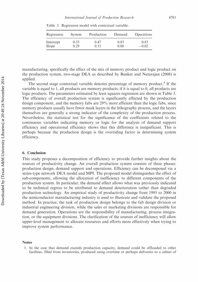
The second stage contextual variable denotes percentage of memory product.4 If thevariable is equal to 1, all products are memory products; if it is equal to 0, all products arelogic products. The parameters estimated by least squares regression are shown in Table 3.The efficiency of overall production system is significantly affected by the productiondesign component, and the memory fabs are 29% more efficient than the logic fabs, sincememory products usually have fewer mask layers in the lithography process, and the layersthemselves are generally a strong indicator of the complexity of the production process.Nevertheless, the statistical test for the significance of the coefficients related to thecontinuous variables indicating memory or logic for the analysis of demand supportefficiency and operational efficiency shows that this difference is insignificant. This isperhaps because the production design is the overriding factor in determining systemefficiency.
6. Conclusion
This study proposes a decomposition of efficiency to provide further insights about thesources of productivity change. An overall production system consists of three phases:production design, demand support and operations. Efficiency can be decomposed via aseries-type network DEA model and MPI. The proposed model distinguishes the effect ofsub-components, allowing the allocation of inefficiency to different components of theproduction system. In particular, the demand effect allows what was previously indicatedto be technical regress to be attributed to demand deterioration rather than degradedproduction technology. An empirical study of productivity change from 1995 to 2000 inthe semiconductor manufacturing industry is used to illustrate and validate the proposedmethod. In practice, the task of production design belongs to the fab design division orindustrial engineering division, while the sales or marketing divisions are responsible fordemand generation. Operations are the responsibility of manufacturing, process integra-tion, or the equipment divisions. The clarification of the sources of inefficiency will allowupper-level management to allocate resources and efforts more effectively when trying toimprove system performance.
Notes
1. In the case that demand exceeds production capacity, demand could be offloaded to otherfacilities, filled from inventories, produced using overtime or perhaps deliveries to a subset of
Table 3. Regression model with contextual variable.
Regression System Production Demand Operations
Intercept 0.33 0.47 0.85 0.83Slope 0.29 0.31 0.08 �0.02
International Journal of Production Research 4781
Dow
nloa
ded
by [
Tex
as A
&M
Uni
vers
ity L
ibra
ries
] at
20:
49 2
4 N
ovem
ber
2014
customers could be renegotiated to postpone the due date. This is necessary because pushingmore raw materials into the system will only increase the product cycle time. In an idealproduction system, the facility is designed to minimise the sum of the expected profit losses fromincrease costs related to excess demand and costs characterising utilisation loss due to lack ofdemand.
2. If non-network DEA is applied, the production system is modelled as a black box and therelationship among sub-components is not considered. Then, the efficiency estimates will belarger than those estimated by rational network DEA. Additional results using non-networkDEA are available from the authors upon request.
3. The 10th fab in the data set, fab 3, switched from memory to logic products in second quarter1996. Thus, we include observations of fab 3 prior to the second quarter in the memory group,and include later observations in the logic group.
4. Due to the data gathering process, outliers or errors in measurement are believed to be aninsignificant concern. However, methods such as that described in Johnson and McGinnis(2008) can be used if these issues are a concern.
References
Banker, R.D., 1993. Maximum likelihood, consistency and data envelopment analysis: a statistical
foundation. Management Science, 39 (10), 1265–1273.Banker, R.D. and Natarajan, R., 2008. Evaluating contextual variables affecting productivity using
data envelopment analysis. Operations Research, 56 (1), 48–58.Caves, D.W., Christensen, L.R., and Diewert, W.E., 1982. The economic theory of index numbers
and the measurement of input, output, and productivity. Econometrica, 50 (6), 1393–1414.Chang, D.S., Kuo, Y.C., and Chen, T.Y., 2008. Productivity measurement of the manufacturing
process for outsourcing decisions: the case of a Taiwanese printed circuit board manufacturer.
International Journal of Production Research, 46 (24), 6981–6995.
Chang, S.Y. and Chen, T.H., 2008. Performance ranking of Asian lead frame firms: a slack–based
method in data envelopment analysis. International Journal of Production Research, 46 (14),
3875–3885.Charnes, A., Cooper, W.W., and Rhodes, E., 1978. Measuring the efficiency of decision making
units. European Journal of Operational Research, 2 (6), 429–444.Charnes, A., et al., 1985. A developmental study of data envelopment analysis in measuring the
efficiency of maintenance units in the U.S. air forces. Annals of Operations Research, 2 (1),
95–112.
Chen, W.C. and McGinnis, L.F., 2007. Reconciling ratio analysis and DEA as performance
assessment tools. European Journal of Operational Research, 178 (1), 277–291.Cook, D.D., Kieschnick, R., and McCullough, B.D., 2008. Regression analyses of proportions in
finance with self selection. Journal of Empirical Finance, 15 (5), 860–867.
Diewert, W.E., 1992. The measurement of productivity. Bulletin of Economic Research, 44 (3),
163–198.Fare, R.S. and Grosskopf, S., 1996. Intertemporal production frontiers: with dynamic DEA. Boston:
Kluwer Academic Publishers.
Fare, R.S., et al., 1992. Productivity changes in Swedish pharmacies 1980–1989: A non-parametric
Malmquist approach. Journal of Productivity Analysis, 3 (1), 85–101.Fare, R.S., et al., 1994. Productivity growth technical progress, and efficiency change in
industrialised countries. American Economic Review, 84 (1), 66–83.
Farrell, M.J., 1957. The measurement of productive efficiency. Journal of the Royal Statistical
Society, Series A, 120 (3), 253–290.Fielding, G.J., Babitsky, T.T., and Brenner, M.E., 1985. Performance evaluation for bus transit.
Transportation Research Part A, 19 (1), 73–82.
4782 C.-Y. Lee and A.L. Johnson
Dow
nloa
ded
by [
Tex
as A
&M
Uni
vers
ity L
ibra
ries
] at
20:
49 2
4 N
ovem
ber
2014

Førsund, F.R. and Hjalmarsson, L., 1987. Analyses of industrial structure: a putty-clay approach.
Industrial Institute for Economic and Social Research, Stockholm: Almqvist and Wicksell
International.Hoff, A., 2007. Second stage DEA: Comparison of approaches for modelling the DEA score.
European Journal of Operational Research, 181 (1), 425–435.Hopp, W. and Spearman, M., 2001. Factory physics. 2nd ed. Boston, MA: Irwin McGraw-Hill.
Johnson, A.L. and McGinnis, L.F., 2008. Outlier detection in two-stage semiparametric DEA
models. European Journal of Operational Research, 187 (2), 629–635.
Johnson, A.L. and Kuosmanen, T., 2009. How do operational conditions and practices effect
productive performance? Efficient nonparametric one-Stage estimators. Working Paper.
Available from: http://ssrn.com/abstract=1485733 [3 November 2009].Kao, C., 2009. Efficiency decomposition in network data envelopment analysis: A relational model.
European Journal of Operational Research, 192 (3), 949–962.Lan, L.W. and Lin, E.T.J., 2005. Measuring railway performance with adjustment of environmental
effects, data noise and slacks. Transportmetrica, 1 (2), 161–189.Leachman, R.C., Ding, S., and Chien, C.F., 2007. Economic efficiency analysis of wafer fabrication.
IEEE Transactions on Automation Science and Engineering, 4 (4), 501–512.
Lovell, C.A.K., 2003. The decomposition of Malmquist productivity indexes. Journal of Productivity
Analysis, 20 (3), 437–458.
Lu, W.M. and Hung, S.W., 2010. Assessing the performance of a vertically disintegrated chain by
the DEA approach – a case study of Taiwanese semiconductor firms. International Journal of
Production Research, 48 (4), 1155–1170.McDonald, J., 2009. Using least squares and tobit in second stage DEA efficiency analyses.
European Journal of Operational Research, 197 (2), 792–798.Nishimizu, M. and Page, J.M., 1982. Total factor productivity growth, technological progress and
technical efficiency: Dimensions of productivity change in Yugoslavia, 1965–78. The Economic
Journal, 92 (368), 920–936.Papke, L.E. and Wooldridge, J.M., 1996. Econometric methods for fractional response variables
with an application to 401(k) plan participation rates. Journal of Applied Econometrics, 11 (6),
619–632.Ray, S.C. and Desli, E., 1997. Productivity growth, technical progress, and efficiency change in
industrialised countries: Comment. The American Economic Review, 87 (5), 1033–1039.Ray, S.C., 1988. Data envelopment analysis, nondiscretionary inputs and efficiency: an alternative
interpretation. Socio-Economic Planning Sciences, 22 (4), 167–176.Ray, S.C., 1991. Resource-use efficiency in public schools: A study of Connecticut data.
Management Science, 37 (12), 1620–1628.Simar, L. and Wilson, P.W., 2007. Estimation and inference in two-stage, semi-parametric models of
production processes. Journal of Econometrics, 136 (1), 31–64.Shephard, R.W., 1953. Cost and production functions. Princeton: Princeton University Press.Sueyoshi, T. andAoki, S., 2001. A use of a nonparametric statistic forDEA frontier shift: TheKruskal
and Wallis Rank Test. OMEGA: International Journal of Management Science, 29 (1), 1–18.Sueyoshi, T. and Goto, M.S., 2001. Slack-adjusted DEA for time series analysis: performance
measurement of Japanese electric power generation industry in 1984–1993. European Journal
of Operational Research, 133 (2), 232–259.Tulkens, H. and Vanden Eeckaut, P., 1995. Non-parametric efficiency, progress and regress
measures for panel data: Methodological aspects. European Journal of Operational Research,
80 (3), 474–499.
White, H., 1980. A heteroskedastic-consistent covariance matrix estimator and a direct test for
heteroskedasticity. Econometrica, 48 (4), 817–838.Yu, M.M. and Lin, E.T.J., 2008. Efficiency and effectiveness in railway performance using a multi-
activity network DEA model. OMEGA: The International Journal of Management Science,
36 (6), 1005–1017.
International Journal of Production Research 4783
Dow
nloa
ded
by [
Tex
as A
&M
Uni
vers
ity L
ibra
ries
] at
20:
49 2
4 N
ovem
ber
2014
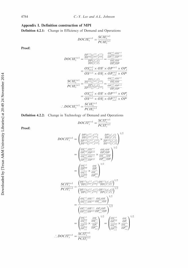
Appendix I. Definition construction of MPI
Definition 4.2.1: Change in Efficiency of Demand and Operations
DOCIEtþ1t ¼
SCIEtþ1t
PCIEtþ1t
Proof:
DOCIEtþ1t ¼
DPtþ1ð y tþ1,xtþ1Þ
DStþ1ð y tþ1, xtþ1Þ
DPtð yt,xtÞDStð yt, xtÞ
¼
OStþ1tþ1=OStþ1
OPtþ1tþ1=OPtþ1
OStt=OSt
OPtt=OPt
¼OStþ1
tþ1 �OSt �OPtþ1 �OPtt
OStþ1 �OStt �OPtþ1
tþ1 �OPt
SCIEtþ1t
PCIEtþ1t
¼
DStð yt, xtÞDStþ1ð y tþ1, xtþ1Þ
DPtð yt,xtÞDPtþ1ð y tþ1,xtþ1Þ
¼
OStþ1tþ1=OStþ1
OStt=OSt
OPtþ1tþ1=OPtþ1
OPtt=OPt
¼OStþ1
tþ1 �OSt �OPtþ1 �OPtt
OStþ1 �OStt �OPtþ1
tþ1 �OPt
;DOCIEtþ1t ¼
SCIEtþ1t
PCIEtþ1t
Definition 4.2.2: Change in Technology of Demand and Operations
DOCITtþ1t ¼
SCITtþ1t
PCITtþ1t
Proof:
DOCITtþ1t ¼
DPtð y tþ1,x tþ1Þ
DStð y tþ1, xtþ1Þ
DPtþ1ð y tþ1,xtþ1Þ
DStþ1ð y tþ1, xtþ1Þ
�
DPtð yt,xtÞDStð yt, xtÞ
DPtþ1ð yt ,xtÞDStþ1ð yt, xtÞ
0@
1A
1=2
¼
OStþ1t =OStþ1
OPtþ1t =OPtþ1
OStþ1tþ1=OStþ1
OPtþ1tþ1=OPtþ1
�
OStt=OSt
OPtt=OPt
OSttþ1=OSt
OPttþ1=OPt
0B@
1CA
1=2
¼
OStþ1t
OP tþ1t
OStþ1tþ1
OPtþ1tþ1
�
OStt
OPtt
OSttþ1
OPttþ1
0B@
1CA
1=2
SCITtþ1t
PCITtþ1t
¼
DStþ1ð y tþ1, xtþ1Þ
DStð y tþ1, xtþ1Þ
DStþ1ð yt,xtÞDStð yt,xtÞ
� �1=2DPtþ1ð y tþ1, xtþ1Þ
DPtð y tþ1, xtþ1Þ
DPtþ1ð yt ,xtÞDPtð yt,xtÞ
� �1=2
¼
OStþ1t =OStþ1
OStþ1tþ1=OStþ1
OStt=OSt
OSttþ1=OSt
� �1=2
OPtþ1t =OPtþ1
OPtþ1tþ1=OPtþ1
OPtt=OPt
OPttþ1=OPt
� �1=2
¼
OStþ1t
OStþ1tþ1
OPtþ1t
OP tþ1tþ1
�
OStt
OSttþ1
OPtt
OPttþ1
0B@
1CA
1=2
¼
OStþ1t
OP tþ1t
OStþ1tþ1
OPtþ1tþ1
�
OStt
OPtt
OSttþ1
OPttþ1
0B@
1CA
1=2
;DOCITtþ1t ¼
SCITtþ1t
PCITtþ1t
4784 C.-Y. Lee and A.L. Johnson
Dow
nloa
ded
by [
Tex
as A
&M
Uni
vers
ity L
ibra
ries
] at
20:
49 2
4 N
ovem
ber
2014
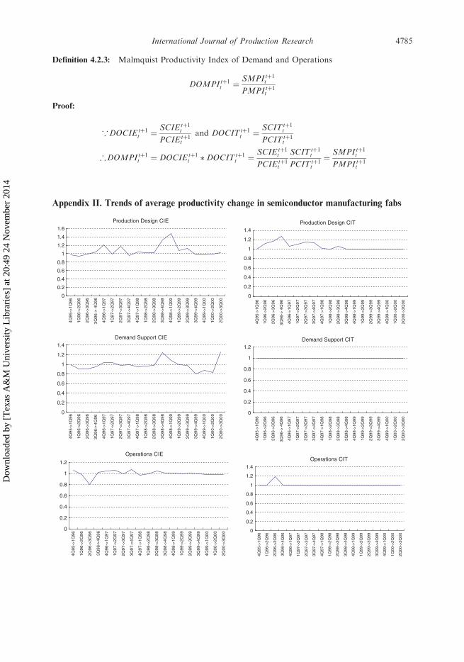
Definition 4.2.3: Malmquist Productivity Index of Demand and Operations
DOMPItþ1t ¼SMPI tþ1t
PMPI tþ1t
Proof:
,DOCIEtþ1t ¼
SCIEtþ1t
PCIEtþ1t
and DOCITtþ1t ¼
SCITtþ1t
PCITtþ1t
;DOMPItþ1t ¼ DOCIEtþ1t �DOCITtþ1
t ¼SCIEtþ1
t
PCIEtþ1t
SCITtþ1t
PCITtþ1t
¼SMPI tþ1t
PMPI tþ1t
Appendix II. Trends of average productivity change in semiconductor manufacturing fabs
Production Design CIE
0
0.2
0.4
0.6
0.8
1
1.2
1.4
1.6
4Q
95-
>1Q
96
1Q
96-
>2Q
96
2Q
96-
>3Q
96
3Q
96-
4Q96
4Q
96-
>1Q
97
1Q
97-
>2Q
97
2Q
97-
>3Q
97
3Q
97-
>4Q
97
4Q
97-
>1Q
98
1Q
98-
>2Q
98
2Q
98-
>3Q
98
3Q
98-
>4Q
98
4Q
98-
>1Q
99
1Q
99-
>2Q
99
2Q
99-
>3Q
99
3Q
99-
>4Q
99
4Q
99-
>1Q
00
1Q
00-
>2Q
00
2Q
00-
>3Q
00Production Design CIT
0
0.2
0.4
0.6
0.8
1
1.2
1.4
4Q95
->1Q
96
1Q96
->2Q
96
2Q96
->3Q
96
4Q9
6
4Q96
->1Q
97
1Q97
->2Q
97
2Q97
->3Q
97
3Q97
->4Q
97
4Q97
->1Q
98
1Q98
->2Q
98
2Q98
->3Q
98
3Q98
->4Q
98
4Q98
->1Q
99
1Q99
->2Q
99
2Q99
->3Q
99
3Q99
->4Q
99
4Q99
->1Q
00
1Q00
->2Q
00
2Q00
->3Q
00
Demand Support CIE
0
0.2
0.4
0.6
0.8
1
1.2
1.4
4Q
95-
>1Q
96
1Q
96-
>2Q
96
2Q
96-
>3Q
96
3Q
96-
4Q96
4Q
96-
>1Q
97
1Q
97-
>2Q
97
2Q
97-
>3Q
97
3Q
97-
>4Q
97
4Q
97-
>1Q
98
1Q
98-
>2Q
98
2Q
98-
>3Q
98
3Q
98-
>4Q
98
4Q
98-
>1Q
99
1Q
99-
>2Q
99
2Q
99-
>3Q
99
3Q
99-
>4Q
99
4Q
99-
>1Q
00
1Q
00-
>2Q
00
2Q
00-
>3Q
00
Demand Support CIT
0
0.2
0.4
0.6
0.8
1
1.2
4Q
95-
>1Q
96
1Q
96-
>2Q
96
2Q
96-
>3Q
96
3Q96
-4Q
96
4Q
96-
>1Q
97
1Q
97-
>2Q
97
2Q
97-
>3Q
97
3Q
97-
>4Q
97
4Q
97-
>1Q
98
1Q
98-
>2Q
98
2Q
98-
>3Q
98
3Q
98-
>4Q
98
4Q
98-
>1Q
99
1Q
99-
>2Q
99
2Q
99-
>3Q
99
3Q
99-
>4Q
99
4Q
99-
>1Q
00
1Q
00-
>2Q
00
2Q
00-
>3Q
00
Operations CIE
0
0.2
0.4
0.6
0.8
1
1.2
4Q
95-
>1Q
96
1Q
96-
>2Q
96
2Q
96-
>3Q
96
3Q
96-
4Q96
4Q
96-
>1Q
97
1Q
97-
>2Q
97
2Q
97-
>3Q
97
3Q
97-
>4Q
97
4Q
97-
>1Q
98
1Q
98-
>2Q
98
2Q
98-
>3Q
98
3Q
98-
>4Q
98
4Q
98-
>1Q
99
1Q
99-
>2Q
99
2Q
99-
>3Q
99
3Q
99-
>4Q
99
4Q
99-
>1Q
00
1Q
00-
>2Q
00
2Q
00-
>3Q
00
Operations CIT
0
0.2
0.4
0.6
0.8
1
1.2
1.4
4Q95
->1
Q96
1Q96
->2
Q96
2Q96
->3
Q96
3Q96
-4
Q96
4Q96
->1
Q97
1Q97
->2
Q97
2Q97
->3
Q97
3Q97
->4
Q97
4Q97
->1
Q98
1Q98
->2
Q98
2Q98
->3
Q98
3Q98
->4
Q98
4Q98
->1
Q99
1Q99
->2
Q99
2Q99
->3
Q99
3Q99
->4
Q99
4Q99
->1
Q00
1Q00
->2
Q00
2Q00
->3
Q00
3Q
96-
International Journal of Production Research 4785
Dow
nloa
ded
by [
Tex
as A
&M
Uni
vers
ity L
ibra
ries
] at
20:
49 2
4 N
ovem
ber
2014