A Deep Learning Approach to Genomics Data for

Population Scale Clustering and Ethnicity Prediction

Md. Rezaul Karim, Achille Zappa, Ratnesh Sahay and Dietrich Rebholz-Schuhmann

Insight Centre for Data Analytics, National University of Ireland, Galway

Email: {firstname.lastname}@insight-centre.org

Abstract. The understanding of variations in genome sequences assists us in identifying people who are predisposed to common diseases, solving rare diseases, and finding

corresponding population group of the individuals from a larger population group.

Although classical machine learning techniques allow the researchers to identify groups or clusters of related variables, accuracies, and effectiveness of these methods diminish

for large and hyperdimensional datasets such as whole human genome. On the other hand,

deep learning (DL) can make better representations of large-scale datasets to build models to learn these representations very extensively. Furthermore, Semantic Web (SW)

technologies already acted as useful adaptors in life science research for large-scale data

integration and querying. Thus the standardized public data created using SW plays an increasingly important role in life sciences research. In this paper, we propose a novel and

scalable genomic data analysis towards population scale clustering and predicting

geographic ethnicity using SW and DL-based technique. We used genotypes data from the 1000 Genome Project resulting from the whole genomes sequencing extracted from

the 2504 individuals consisting of 84 million variants with 26 ethnic origins.

Experimental results in terms accuracy and scalability show the effectiveness and superiority compared to the state-of-the-art. Particularly, our deep-learning-based

analytics technique using classification and clustering algorithms can predict and group

targeted populations with a prediction accuracy of 98% and an ARI of 0.92 respectively.

Keywords: Population Genomics, 1000 Genome Project, Genotype Clustering,

Genotype Classification, Deep Learning, Semantic Web.

1 Introduction

Over the last few years, life sciences have seen a rapid reduction in costs and time

after the completion of the next generation genome sequencing (NGS). Research in

this area is also entering into the big data space since datasets from numerous sources

are being produced in an unprecedented way after the completion of whole genome

sequencing. Analyzing these large-scale data is computationally expensive. This

drastic increase in NGS for both sample numbers and features per sample requires a

massively parallel approach to data processing which imposes great challenges to the

machine learning algorithms and bioinformatics tools. Since the genomic information

is increasingly used in medical practice, it is giving rise to the need for efficient

analysis methodology able to be able to cope with thousands of individuals and

millions of variants [1]. A commonly performed task in such applications is grouping

individuals based on their genomic profile to identify population association or

elucidate haplotype involvement in diseases susceptibility.

The 1000 Genome Project [2] is an example of genome-wide Single Nucleotide

Polymorphisms (SNPs) for predicting ancestry at continental and regional scales. It

2

also shows that population group from Asia, Europe, Africa and America are clearly

distinguishable based on the human races and genomic data. However, accurate

prediction of haplogroup and continent of origin geography, ethnicity, and language

are more challenging. Research has also argued that till date, many Y chromosome

lineages are geographically localized and thus there still have strong evidence of

clustering human allele from human genotypes. Now we have several research

questions that need to be addressed: i) how are the human genetic variations

distributed geographically among groups of populations? ii) Is it possible to group the

individuals based on their genomic profile to identify population association or

elucidate haplotype involvement in diseases susceptibility? iii) Is it possible to use

the genomic data to predict geographic origin (i.e. which population group an

individual belongs to) from an individual’s sample?

DL is a branch of machine learning (ML) based on a set of algorithms that attempt

to model high-level abstractions in data [3]. Research in this area attempts to make

better representations and create models to learn these representations extensively

from large-scale labeled or unlabeled data compared to the classical ML models. Life

science is no exception, but DL in this area is a radical combination that has created

some great impacts in NGS data analytics. Consequently, a similar concept has been

used in probabilistic graphical models [4] and using the deep belief networks for

prognosis of breast cancer [5] and in multi-level gene/miRNA feature selection using

deep belief networks [6]. Thus to answer the above questions, based on the genomic

data, it is possible to build DL models to classify or clusters the genomes by the

populations itself. It can be observed that the populations are reconstructed in the DL

model in a supervised (e.g. classification) or unsupervised (e.g. clustering) ways

towards predicting ethnic groups. Moreover, a DL model can be built to infer the

missing genotypes.

On the other hand, SW technologies connect humans with data by adding human-

readable labels to datasets and formalizing facts as axiomatic statements.

Bioinformatics solutions already employed SW technologies since these technologies

already acted as an early adaptor in life science research for large-scale data

integration and querying enabling data access in distributed and heterogeneous

environments [7-9]. Furthermore, data from the various genomics projects such as

NGS, 1000 Genome Project and Personal Genome Project (PGP) [10] are large-scale.

Therefore, to address the scalability issues and for faster processing on these data,

ADAM and Spark-based [11-13] solutions have been popular and are now being used

in genomics widely [13, 14]. Spark’s in-memory cluster computing framework [15,

16] allows user programs to persist data into memory repeatedly, making it well-

suited for the ML algorithms.

In this paper, we show how to address the above questions in a scalable and faster

way. Particularly, we explain how to apply SW for the data integration and querying,

Spark and ADAM for data processing and H2O [17] for DL APIs to accurately

predict which population group an individual belongs to from individual’s genomic

data. Secondly, also carried out population scale clustering of in inter and intra-super

population groups. The primary contributions of our paper can be summarized as

follows:

We propose a novel approach to analyze geographic population scale from

the 1000 Genome Project. Same technique can predict the geographic ethnic

groups from unknown genotypic datasets as well

Our approach is based on a combined technique of SW, ADAM, Spark and

DL which is not only scalable and accurate but also shows consistent

performance against all the genotypic dataset consisting of all the

chromosomes from the 1000 Genome Project

Experimental results in terms of accuracy and scalability show the

effectiveness of our approach. Our deep-learning-based clustering technique

using K-means algorithm can group the populations with high accuracy with

WSSSE of only 1.2% and can cluster the whole genome in only 15h with an

ARI of 0.92. Whereas, the DL-based classifier can predict the population

groups with an MSE of 4.9%, an accuracy of 95%, the precision of 94%,

recall of 93% and an f1 measure of 93%. Overall, our approach is scalable

seamlessly from 10% to 100% of the whole human genome.

We also showed that the inferred features from the genotypic data provide

higher classification and clustering accuracy compared to the state-of-the-art

like ADMIXTURE [18, 19] and VariationSpark [1].

The rest of the paper is structured as follows: Section 2 briefly describes the 1000

Genome project and related dataset. Section 3 discusses the material and the methods

of our approach. Section 4 discusses the experimental results. In section 5, we discuss

some related works. Finally, we conclude our paper in section 6.

2 The 1000 Genome Project

Data from the 1000 Genome Project is a deep catalog of human genetic variations

[18] that are widely used to screen variants discovered in exome data from individuals

with genetic disorders and in cancer genomic projects. The goal of the project was to

find most genetic variants with frequencies of at least 1% in the populations studied.

Data from the 1000 Genomes Project was quickly made available to the worldwide

scientific community through freely accessible public data repositories.

The phase 3 of the project contains data from the 2,504 samples were combined to

allow highly accurate assignment of the genotypes in each sample at all the variant

sites. All donors were over 18 and declared themselves to be healthy at the time of

collection. Since any particular region of the genome generally contains a limited

number of haplotypes, the genomic data was combined across samples to allow

efficient detection of most of the variants in a region. However, only the Illumina

platform data with 70bp reads or longer are used. Moreover, a newer method is

developed to integrate information across several algorithms and diverse data sources

with a broad spectrum of genetic variation [19]. The multi-sample approach combined

with genotype imputation allowed the project to determine a sample’s genotype, even

invariants not covered by sequencing reads in that sample. Moreover, all individuals

were sequenced using both whole-genome sequencing with mean depth = 7.4x and

targeted exome sequencing with the mean depth of 65.7x. In addition, individuals and

4

available first-degree relatives such as adult offspring were genotyped using high-

density SNP microarrays. Table 1 shows the statistics of the dataset that we used.

Table 1. Statistics of the dataset from the 1000 Genome Project (Release 3) used for our study

1000 Genome release Variants Individual Populations Size

Phase 3 84.4 million 2504 26 820GB

It is to be noted that the allele frequency in the EAS, EUR, AFR, AMR and SAS

populations is calculated from AC and AN with all are in the range of (0, 1). Research

has shown that individuals from different populations carry different profiles of rare

and common variants, and that low-frequency variants show substantial geographic

differentiation which is further increased by the action of purifying selection.

The 1000 Genome project started in 2008 with the help of a consortium consisting

of more than 400 life scientist and the phase 3 finished in September 2014 with 26

populations from 2504 individuals. Total over 88 million variants (84.7 million single

nucleotide polymorphisms (SNPs), 3.6 million short insertions/deletions (indels), and

60,000 structural variants) were phased onto high-quality haplotypes characterized

[18]. Later on, some less important variants including SNPs, indels, deletions,

complex short substitutions and other structural variant classes were removed that did

not pass the QC. As a result, the phase 3 release leaves the data from the 2504

individuals from 26 different populations consisting of total 84.4 million variants.

Note that 99.9% of variants consist of SNPs and short indels [2]. Each of the 26

populations has about 60-100 individuals from Europe, Africa, America (south and

north) and Asia (South and East).

In short, the genotypes consisting of the genotypes data of 23 chromosomes and a

panel file that are downloaded from the 1000 Genome project are used in our study.

For analysis, populations are grouped into 5 super population groups by the

predominant component of ancestry: East Asian (CHB, JPT, CHS, CDX, and KHV),

Europe (CEU, TSI, FIN, GBR, and IBS), Africa (YRI, LWK, GWD, MSL, ESN,

ASW, and ACB), Americas (MXL, PUR, CLM, and PEL) and the South Asian (GIH,

PJL, BEB, STU and ITU) as shown in Figure 1. Table 1 shows related statistics of the

dataset used in our study.

3 Materials and Methods

In this section, a brief description of the data pre-processing, RDFization and feature

extractions will be discussed. Finally, training methodology of the DL models will be

discussed.

3.1 Getting the dataset from VCF to CSV format

The dataset from the Phase 3 contributed about 820GB of data meaning a large-scale

data. Therefore, ADAM and Spark are used to pre-process and prepare the data for

the DL model (i.e. training, testing, and validation set) in a scalable and faster way.

After that, K-means and the classifier models (from the H2O) are trained for the

clustering and classification respectively for analyzing the population group of an

individual. The Sparking Water is used to make the data conversion interoperable

between H2O and Spark. Table 2 lists the technologies that were used in our study.

Table 2. Technology used in our study

Tool/Technology Purpose

ADAM Is used as genomics analysis platform to avail the support for the associated

file formats (i.e. VCF) and scalable API for genome data processing. Apache Spark This is the fastest engine for large-scale data processing used for three

purposes: i) for converting ADAM DataFrame to Spark DataFrame, ii) Spark

DataFrame to CSV format and iii) from RAW SPARQL query results to back

Spark DataFrame before feeding by the H2O.

Semantic Web We extended the Jena API to converting CSV to RDF in N3 format. SPARQL

is used to query the RDF data to get only the selected features to train the DL models. Then the resulting raw data file is converted into Spark DataFrame.

H2O/Sparkling

Water

Is used as the predictive analytics platform for DL. Before training the DL

model, Spark DataFrame is further converted into H2O DataFrame. The Sparkling Water provides the support for the integration of H2O with Spark.

The genotype dataset in Variant Call Format (VCF) contains the data about a set of

individuals (aka. samples) and their genetic variations. The panel file lists the

population group (aka. region) for each sample in the genotype file which is the

response column (aka. predicted column) that we want to predict eventually. This is a

tab-delimited (aka.TSV) file containing samples and populations respectively in the

first two columns. Some VCF file against chromosome may also have subsequent

columns that describe additional information like which super population a sample

comes from or what sequencing platforms have been used to generate sequence data

for that individual.

However, for our clustering and classification analysis, we considered all the

genotypic information of each sample using the sample ID, variation ID and the count

of the alternate alleles. The majority of variants that we used are SNPs and indels.

Now before training a clustering or classification model, we first prepared the

training, test and validation set in such a way that they can be consumed by the DL

models. At first, we read the Panel file using ADAM and Spark to map with the target

population selected by the users and then filtering is applied on it based on the

population groups in the populations set. The Panel file contains only the sample ID

in the first column and the population group in the second column. A sample of the

panel file is shown in Table 3.

Table 3. Technology used in our study

Sample ID Pop Group Ethnicity Super pop. group Gender Sample ID

HG00096 GBR British in England and Scotland

EUR male HG00096

HG00171 FIN Finnish in Finland EUR female HG00171

HG00472 CHS Southern Han Chinese EAS male HG00472

HG00551 PUR Puerto Ricans from

Puerto Rico

AMR female HG00551

ADAM and Spark help us in filtering the genotype data to contain only samples

that are in the population groups that we are interested (selected by the user coming

6

from the panel file containing all the information of individual and super population

groups) into a single genotype object. Then the genotype object is converted into a

SampleVariant object. This object contains just the data we need for further

processing: the sample ID that uniquely identifies a particular sample, a variant ID

that uniquely identifies a particular genetic variant and a count of alternate alleles

only when the sample differs from the reference genome. These variations help us to

classify individuals according to their population group.

A total number of samples or individuals in the data is then counted before

grouping them using the variant IDs and filtering out those variants that do not appear

in all of the samples. The aim of this is to simplify the pre-processing of the data.

Target is to handle a very large number of variants in the data that is around 84

million depending on the exact dataset. It is to be noted that filtering out a small

number of variants will not make a significant difference to the results and hence, we

can reduce the number of variants even further. Since a dataset contains very large

numbers of features, particularly if the number of samples is relatively small, we first

need to try and reduce the number of variants in the data.

However, we did not utilize any third-party dimensionality reduction algorithms

but Spark core library. We first computed the frequency with which alternate alleles

have occurred for each variant and those variants that appear within a certain

frequency range are filtered out. In this case, we have chosen a fairly arbitrary

frequency count of 11. This was chosen through some previous literature as suggested

in the 1000 Genome Project website. This results and leaves around 3 million variants

in the dataset we are using (for 23 files). Spark is then used to convert ADAM

DataFrame (i.e. SampleVariant objects) to Spark DataFrame. After that Spark

DataFrame is further converted to CSV format for making the RDFization easier.

3.2 RDFization and feature extraction

We gathered all data sets into the Resource Description Format (RDF). The formal

specification of RDF is convenient, as it allows for the integration of data while

preserving their original semantics. This uniform format allows for the easy

combination of these resources that can help to get different viewpoints on genomics

facts within one interlinked resource knowledge graph, an increasingly used umbrella

term for loosely structured graph-based knowledge representation. Once all the Spark

DataFrames are converted into a uniform (i.e. CSV) format, we then RDFized them

(i.e. 23 chromosomes in CSV format). Our in-house RDFizer tool is used for the

RDFization. The tool that we developed for the RDFization is using Spark written in

Java that extends Apache Jena API. The CSV RDFizer takes the tab separated text

files as input and generates the resulting RDF files in the form of N3 triples. We

would like to argue about the N3 triples since it generates the data in more compact

formats. Since the 1000 Genome Project data for 23 chromosomes are huge (i.e. Big

Data), we packaged our Spark application with all the required dependencies as Java

jar and transferred it to the database server. After that, we submitted the Spark job for

the RDFization on the data server side itself without moving the data home.

Table 2 shows related statistics of the RDF datasets. It is to be noted that based on

the opinion of a domain expert, we have identified only the potential and required

data fields (records) before assigning them URIs and prefixes for the values from

those fields. We used our RDF data model to make the whole RDFization process

consistent across all the raw files for the URIs, base URIs, prefixes and corresponding

values. The resulting RDF dataset is only 90GB since we have considered only some

selected features. In short, out of the 23 chromosomes, our CSV RDFizer generates

exactly 23 N3 files as RDF under a common graph. We then configured Apache Jena

Fuseki server1 and uploaded the resulting RDF data which results in around 1.6

billion triples as shown in Table 4.

Table 4. RDF dataset statistics from the 1000 Genome Project (phase 3)

Chromosome Triples (million) Size (Compressed, MB)

1 105.4 1180

2 123.7 1260

3 100.1 1050

4 100.2 1060

5 91.54 910

6 92.43 930

7 86.54 850

8 84.23 810

9 71.58 620

10 75.65 710

11 74.13 700

12 72.87 680

13 63.87 500

14 58.42 440

15 54.0 400

16 57.09 430

17 49.86 380

18 48.0 370

19 42.57 310

20 40.64 290

21 30.13 210

22 28.63 200

X 25.0 178

Y 0.08 5

Total 1.58 Raw 15GB, Uncompressed 820 GB

Then before training the DL models (clustering and classification), we retrieve

required features such as sample ID that uniquely identifies a particular sample, a

variant ID that uniquely identifies a particular genetic variant, position id, RS id, the

count of alternate alleles using the SPARQL query. Alleles in our study are important

because they account for the differences in inherited characteristics from one

individual to another. A sample query that retrieves the sample id, variant id, position

id, RS id and variants from chromosome 22 is shown in listing 1 and figure 1 shows

the conceptual view of feature extraction from the 1000 Genome Project dataset.

8

PREFIX pop_genomics: <http://genomics.sels.insight.org/schema/> PREFIX dcterms: <http://purl.org/dc/terms/> PREFIX owl: <http://www.w3.org/2002/07/owl#>

SELECT * WHERE {

?INDV pop_genomics:sample ?sample_ID ; pop_genomics:variants ?variant_ID ; pop_genomics:position ?position_ID ; pop_genomics:rsid ?RS_ID ; pop_genomics:info ?variants .

FILTER(?sample_ID = "ASW" && ?sample_ID = "CHB" && ?sample_ID = "CLM" &&

?sample_ID = "FIN" && ?sample_ID = "GBR") .

FILTER(?INDV =”chr22”) .

}

Listing 1: Feature extraction to train DL models (from chromosome 22 using SPARQL query)

3.3 DL model training, tuning, and evaluation

When we have the features ready extracted from the SPARQL query, later on, we

further convert it back as the H2O data frame to train the DL model –i.e. either

classification or K-means model. To train the models, we need our data to be in a

tabular form where each row represents a single sample and each column represents a

specific variant. However, we further converted the tabular data to sparse vector to

feed the models. Moreover, the table should contain a column (i.e. response column)

for the population group or "Region", which is what we are trying to predict.

Fig. 1. A conceptual view of feature extractions process from the genotype data. Features with sample ID, Variant ID, genetic variant, position id and RS id taken into count that are passed.

Features including sample ID, Variant ID, genetic variant, position id and RS id collected that are passed.

Allele frequency count: Range (0, 1) for the entire super population group (i.e. EAS, EUR, AFR, AMR, SAS) from AC and AN.

Ultimately, in order for our data to be consumed by the H2O, we need to convert it

to an H2O data frame object. We first group the data by the sample ID, and then sort

the variants for each sample in a consistent manner using the variant IDs. After that, a

header row for the table is created containing the Region column, the sample ID and

all of the variants. Then we randomly split the data frame into the training, test and

the validation set. The training set is used to train the model; test set is used to ensure

that the overfitting does not occur and the validation set that performs a similar

purpose to the test set but is used to validate the strength of our model as it is being

built while avoiding overfitting in the DL models.

However, when training a DL model based neural network, we typically keep the

validation set distinct from the test set to enable us to learn hyper-parameters for the

model as suggested by previous literature [3]. When machine learning models are

trained using the clustering (using K-means) or classification (using H2O

classification algorithm), each variant is treated as a "feature" for the model training.

It is to be noted that before training the K-means or classification model, we set the

parameters and specify the training and validation datasets, as well as the column in

the data which contains the item we are trying to predict i.e. in this case, the Region.

We also set some hyper-parameters which affect the way the model learns. H2O also

provides methods for automatically tuning hyperparameters so it may be possible to

achieve better results by employing one of these methods. We trained the supervised

DL model by specifying the number of epochs and the hidden layers and the

activation function was set as rectified with dropout and an epsilon. Moreover, to get

better classification results we also keep the adaptive rate, force load balance, keeping

cross validation splits and over-write with the best model as true.

On the other hand, in general, since we have n data points (features) xi,i=1...n,

therefore, the data points have to be partitioned into K clusters –i.e. K population

groups. Note that it is possible for fewer than k clusters to be returned by the K-means

algorithm. For example, if there are fewer than K distinct points to the cluster. Now

using the K-means the goal is to assign a cluster to each data point. Since K-means is

a clustering method –which means that its aim is to find the position μi,i=1...K of the

clusters that minimize the distance from the data points to the cluster. K-means

clustering algorithm in the H2O tries to minimize the value of the objective function

or cost function that can be adapted from [20] and expressed as follows:

Where ci is the set of points that belong to cluster I and the K-means clustering uses

the square of the Euclidean distance d(x, μi) = ∥x−μi∥22. Since this problem is not a

trivial but NP-hard, therefore the K-means algorithm only hopes to find the global

minimum, possibly getting stuck in a different solution. Considering this constraint in

our proposed method we trained the K-means model using K as the number of

targeted clusters, MaxIterations as the maximum number of iterations to run, epsilon

as the distance threshold within that we consider k-means to have converged and the

initialModel which is an optional set of cluster centers used for initialization.

However, if this parameter is supplied, only one run is performed.

10

4 Results and Discussion

In this section, we will briefly discuss the experimental results. Due to the page

limitation, we are unable to provide details but will analyze the results of the

classification and clustering for only a few of the selected population groups.

4.1 Experimental setup

Tools that are used in the experiment were implemented using heterogeneous

technologies like Spark, ADAM, SW, and DL hence making them scalable and

computationally faster. All programs were written with Scala using Spark MLlib

library and DL from the H2O. The operating system for the cluster was Ubuntu 14.04

64-bit while the version of Spark was 2.1.0, H2O version 3.0.0.8, Sparkling Water

version 1.2.5 and ADAM version was 0.16.0. During the reporting period, we trailed

a cluster of 100 computing cores and 274GB of RAM. We used only 30 computing

cores (with 29 as computing cores and one as the driver program).

4.2 Classification analysis

Having trained the supervised DL model, we now need to check how well it predicts

the population groups against the genotype dataset. To do this, we "score" the entire

data set (including training, test, and validation data) against our model. Drawing a

confusion matrix tells us how well the DL model predicts our targeted population

groups. These specific evaluation metrics for multi-class learning, which are different

from the ones used in traditional supervised learning. Considering we have p

population groups, for each group xi we have a set Y (xi) of actual group prediction

and a set G (xi) of predicted population groups then based on the above formulas, we

computed the performance metrics.

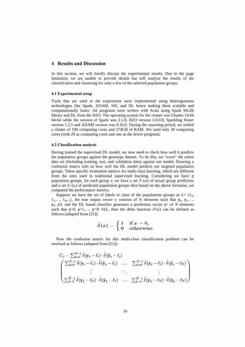
Suppose we have the set of labels or class of the populations groups as L= {ℓ0,

ℓ1,…, ℓM−1}, the true output vector y consists of N elements such that y0, y1,…,

yN−1∈L and the DL based classifier generates a prediction vector y^ of N elements

such that y^0, y^1,…, y^N−1∈L, then the delta function δ^(x) can be defined as

follows (adapted from [21]):

Now the confusion matrix for this multi-class classification problem can be

resolved as follows (adapted from [21]):

Now that based on the above equation and for the following five targeted groups

(i.e., ASW, CHB, CLM, FIN, and GBR) the confusion matrix we got is as follows (to

keep the explanation simpler).

Table 4. Confusion matrix (vertical: actual; across: predicted)

Group ASW CHB CLM FIN GBR Error Rate

ASW 59 0 1 1 0 0.0328 2/61

CHB 0 103 0 0 0 0.0000 0/103

CLM 3 0 86 3 2 0.0851 8/94

FIN 0 0 86 3 2 0.0202 2/99

GBR 0 0 1 9 81 0.1099 10/91

Total 62 103 88 110 85 0.0491 22/448

We trained the DL model with 50 epochs, 150x150 hidden layers, the activation

function was set as rectified with dropout, an epsilon of 0.001 was used to make the

training more intensive. To get the better classification results, we also keep the

adaptive rate, force load balance by keeping the cross validation splits. To get the best

model, we keep over-writing and took only the best model. We calculated the

accuracy, precision, recall and f1 measure for the DL-based multi-class classification

model using the following mathematical formulas adapted from [21] as follows:

With the above setting, our DL based classifier can predict the population groups

with mean squared error (MSE) value of only 4.9%, an accuracy of 95%, a precision

of 95.45%, a recall of 95.60% and the f1 measure of 93.52%. We calculated the MSE

using standard formula used in the DL classifier on the test set adapted from [21] as

follows:

Where n is the number of test samples (448 for 5 population groups), yi is the true

label in the panel file and ^y

i is the predicted label for the 5 population groups. It is to

be noted that for the classification task, predicted labels yi are converted into a

corresponding dense vector representation.

4.3 Cluster analysis

Typical objective functions in clustering formalize the goal of attaining high intra-

cluster similarity and low inter-cluster similarity. This is an internal criterion for the

quality of a clustering. Therefore, we used Rand index (RI) to evaluate the clustering

quality which measures the percentage of decisions that are correct. Later on, the RI

12

was normalized to Adjusted Rand index (ARI) that returned a value between -1

(independent labeling) and 1 (perfect match) [25]. Adjusted for a chance measures

such as ARI display some random variations centered on a mean score of 0.0 for any

number of samples and clusters. Only adjusted measures can hence safely be used as a

consensus index to evaluate the average stability of clustering algorithms for a given

value of K on various overlapping subsamples of the dataset.

The following formula is used to calculate the ARI for evaluating the clustering

quality for our approach and the state-of-the-art like VariationSpark and

ADMIXTURE for the annotated population groups (i.e. 26) and super population

groups (i.e. 5).

Our approach successfully completes the clustering of the whole 820GB of data in

15h with an ARI of 0.92 for clustering. The VariationSpark takes about 32h with an

ARI of 0.82. ADMIXTURE, on the other hand, takes about 35h with an ARI of 0.25.

Note that here we did not include the RDFization and SPARQL query time. The

overall population clustering shows that the genotypes data from AFR, EAS, and

AMR are relatively homogeneous. However, EUR and SAS are more mixed so don’t

scale towards cluster well. Due to the page limitation, we could not show the details

results of the population scale clustering for inter-super population groups.

Fig. 2. Population scale cluster of 5 groups from chr 22 [between actual and predicted (x and y-axis)]

Furthermore, we took the advantage of the Elbow method for determining the

optimal number of clusters to be set prior training the K-means model. We calculated

the cost using Within-cluster Sum of Squares (WCSS) as a function of a number of

clusters for K-means algorithm applied to Genotype data based on all the features of

26 population groups.

5 Related Works

Numerous literature has already been used for the integration and processing of life

science data at scale using SW technologies [7-9]. One of the commonly used tools is

ADMIXTURE [25], which performs maximum likelihood estimation of individual

ancestries from multi-locus SNP genotype datasets. As stated earlier the 1000

Genome Project Consortium developed a global reference for human genetic variation

for exome and genome sequencing. Later on, biological sequence alignment in

distributed computing system as [11] is an example of using Spark for genome

sequence analysis. The resulting tool VariantSpark provides an interface from MLlib

to the standard variant format (VCF) that offers a seamless genome-wide sampling of

variants and provides a pipeline for visualizing results from the 1000 Genome Project

and Personal Genome Project (PGP). However, the overall clustering accuracy is

lower and does not provide any support of classifying the individual based on the

genotypic information.

Various DL architectures, on the other hand, have been shown to produce state-of-

the-art results on various tasks. Consequently, a similar concept has been used in

probabilistic graphical models and using the deep belief networks for prognosis of

breast cancer [15]. DL based technique has also been applied for the multi-level

gene/miRNA feature selection using deep belief nets and active learning [16].

Recognizing the capability, Wiewiórka et al. [18] developed SparkSeq for high-

throughput sequence data analysis. The Big Data Genomics (BDG) group, on the

other hand, demonstrated the strength of Spark in a genomic clustering application

using ADAM for genomic data [20]. While the speedup of ADAM over traditional

methods was impressive for the 50 fold speedup, this general genomics framework

can hamper the prediction performance.

6 Conclusions

In this paper, we applied a Spark, ADAM, SW, and DL based technique to handle

large-scale genomic dataset to achieve outstanding results in a scalable and faster

way. Our approach successfully predicts geographic population groups and is

consistent against all the genotypic dataset consisting of all the chromosomes. We

show that the inferred features from the genotypic data with higher clustering and

classification accuracy in comparison to the state-of-the-art like [1, 2]. Experimental

results in terms of accuracy and scalability show the effectiveness of our approach.

We believe that the same technique can predict the geographic ethnic groups from

unknown genotype datasets as well.

The human genetic diversity tends to be distributed clinically; it is especially

problematic to sample the extremes of continents because this will create the

impression of sharp discontinuities in the distribution of genetic variants. In future,

we will provide more details about analysis on intra-super-population groups and

discuss the homogeneity and heterogeneity among different groups. Secondly, we

intend to extend this work by considering another dataset like PGP and factors like

predicting population groups within larger geographic continents.

14

Acknowledgments

This publication has emanated from research conducted with the financial support of

Science Foundation Ireland (SFI) under the Grant Number SFI/12/RC/2289.

References

1. Aidan R. O’Brien, Neil F. W. Saunders, Yi Guo, Fabian A. Buske, Rodney J. Scott

and Denis C. Bauer, VariantSpark: population scale clustering of genotype

information, BMC Genomics, 201516:1052, DOI: 10.1186/s12864-015-2269-7.

2. The 1000 Genome Project, http://www.internationalgenome.org/data#DataAccess

3. Seonwoo Min, Byunghan Lee, Sungroh Yoon; Deep learning in bioinformatics. Brief

Bioinform 2016 bbw068. doi: 10.1093/bib/bbw068

4. Michael K. K. Leung, Andrew Delong, Babak Alipanahi and Brendan J. Frey,

Machine Learning in Genomic Medicine: A Review of Computational Problems &

Data Sets, Proceedings of the IEEE (V. 104, No. 1, Jan. 2016 )

5. Mahmoud Khademi and Nedialko S. Nedialkov, Probabilistic Graphical Models and

Deep Belief Networks for Prognosis of Breast Cancer, IEEE 14th International

Conference on Machine Learning and Applications (ICMLA).

6. Rania Ibrahim, Noha A. Yousri, Mohamed A. Ismail and Nagwa M. El-Makky,

Multi-level gene/miRNA feature selection using deep belief nets and active learning,

Engineering in Medicine and Biology Society (EMBC), 2014 36th Annual

International Conference of the IEEE

7. Hasnain A., Dunne N., Rebholz-Schuhmann D., Processing Life Science Data at

Scale using Semantic Web Technologies, Tutorial in SWAT4LS: Semantic Web

Applications and Tools for Life Sciences, UK 2015.

8. A Zappa, A Splendiani, P Romano, Towards linked open gene mutations data, BMC

bioinformatics, vol. 13, No. 4, PP. S7, 20212.

9. A Zappa, P Romano – EMBnet, A first RDF implementation of the COSMIC

database on mutations in cancer, EMBnet. Journal, Vol. 18, No. B, Pp. 151-153.

10. Personal Genome Project (PGP), http://www.personalgenomes.org/

11. Matt Massie, Frank Nothaft, Christopher Hartl, Christos Kozanitis et al., ADAM:

Genomics Formats and Processing Patterns for Cloud Scale Computing, EECS

Department University of California, Berkeley Technical Report No. UCB/EECS-

2013-207, December 15, 2013

12. X. Lu, M. W. U. Rahman, N. Islam, D. Shankar, D. K. Panda, Accelerating spark

with Adam for big data processing: Early experiences, in High-Performance

Interconnects (HOTI), 2014 IEEE 22nd Annual Sym. on, IEEE, 2014, pp. 9–16.

13. Dries Harnie, Alexander E. Vapirev, Jörg Kurt Wegner and Andrey Gedich, Scaling

Machine Learning for Target Prediction in Drug Discovery using Apache Spark,

Cluster, Cloud and Grid Computing (CCGrid), 2015 15th IEEE/ACM Intl. Symp.

14. G. Zhao, C. Ling, D. Sun, Sparksw: scalable distributed computing system for large-

scale biological sequence alignment, in Cluster, Cloud and Grid Computing

(CCGrid), 2015 15th IEEE/ACM International Sym. on, IEEE, 2015, pp. 845–852.

15. D. R.-S. MR Karim, R Sahay, A scalable, secure and real-time healthcare analytics

framework with apache-spark, in Proc. of the 2nd INSIGHT student conference on

Data Analytics, The Insight Centre for Data Analytics, 2015, pp. 83–83.

16. M. Zaharia, M. Chowdhury, T. Das, A. Dave, J. Ma, M. McCauley, M. J. Franklin, S.

Shenker, I. Stoica, Resilient distributed datasets: A fault-tolerant abstraction for in-

memory cluster computing, in: Proceedings of the 9th USENIX conf. on Networked

Systems Design and Implementation, USENIX Association, 2012, pp. 2–2.

17. Arno Candel, Jessica Lanford, Erin LeDell, Viraj Parmar and Anisha Arora, Deep

Learning with H2O, http://h2o-release.s3.amazonaws.com/h2o/rel-slater/9/docs-

website/h2o-docs/booklets/DeepLearning_Vignette.pdf

18. ADMIXTURE, https://www.genetics.ucla.edu/software/admixture/

19. Alexander DH, November J, Lange K. Fast model-based estimation of ancestry in

unrelated individuals. Genome Res. 2009; 19(9):1655–64. doi:10.1101/gr.094052.109

20. K-means clustering, http://www.onmyphd.com/?p=k-means.clustering

21. Multiclass classifier, https://spark.apache.org/docs/latest/mllib-evaluation-

metrics.html.