a deep learning approach to identifying household

A Deep Learning Approach to Identifying

Household Appliances from Electricity Data

Zongzuo Wang

TH

E

U N I V E RS

IT

Y

OF

ED I N B U

RG

H

Master of Science

School of Informatics

University of Edinburgh

2016

Abstract

Reduction in energy consumption is becoming increasingly important for both finan-

cial and environmental reasons. Energy disaggregation, which tries to estimate ap-

pliance specific data from whole houses electricity demand, proves to be an efficient

guidance for energy consumption reduction. On the other hand, deep learning has

achieved remarkable success in fields like image classification and speech recognition.

This paper implements an energy disaggregation algorithm based on deep learning and

further optimisation. Multilayer perceptrons, convolutional denoising autoencoders

and long short term memory networks are trained for five appliances. The results are

evaluated using five metrics and compared to similar work. Further optimisations are

carried out upon the network predictions with constraints that the sum of predictions

are no greater than the mains, and power demands are non-negative. The optimisation

results show this method is able to correct and improve the disaggregation results even

further.

iii

Acknowledgements

First of all, I would like to thank my supervisor Dr. Mingjun Zhong, who gave me

so much help and guidance in this project from the beginning to the end. He is a

thoughtful and excellent researcher, he trained me to pay attention to details, and he

is very passionate and open-minded to discuss problems with me. Also, many thanks

to Prof. Nigel Goddard. He gave me a lot of helpful advice on how to write a good

dissertation and what matters in a successful project. I would also like to thank my

partner, Chaoyun Zhang. We often discuss technical questions and exchange ideas.

He inspired me a lot during the project, and generously offered me GPU for network

training. Finally, I would like to thank my parents, who supported me both financially

and mentally with all efforts, and gave me such a great chance to study in this excellent

MSc programme.

iv

Declaration

I declare that this thesis was composed by myself, that the work contained herein is

my own except where explicitly stated otherwise in the text, and that this work has not

been submitted for any other degree or professional qualification except as specified.

(Zongzuo Wang)

v

Table of Contents

1 Introduction 1

1.1 Motivation . . . . . . . . . . . . . . . . . . . . . . . . . . . . . . . . 1

1.1.1 Importance of energy consumption reduction . . . . . . . . . 1

1.1.2 Advantages of providing appliance specific data . . . . . . . . 1

1.1.3 Smart meters . . . . . . . . . . . . . . . . . . . . . . . . . . 2

1.2 Objective . . . . . . . . . . . . . . . . . . . . . . . . . . . . . . . . 2

1.3 Achieved results . . . . . . . . . . . . . . . . . . . . . . . . . . . . . 3

1.4 Dissertation outline . . . . . . . . . . . . . . . . . . . . . . . . . . . 3

2 Background 5

2.1 Relevant work . . . . . . . . . . . . . . . . . . . . . . . . . . . . . . 5

2.1.1 Non-intrusive load monitoring . . . . . . . . . . . . . . . . . 5

2.1.2 Deep learning . . . . . . . . . . . . . . . . . . . . . . . . . . 6

2.2 Inspiration of this project . . . . . . . . . . . . . . . . . . . . . . . . 7

3 Methods 9

3.1 Resource and tools . . . . . . . . . . . . . . . . . . . . . . . . . . . 9

3.2 Data . . . . . . . . . . . . . . . . . . . . . . . . . . . . . . . . . . . 9

3.2.1 UK-DALE data set . . . . . . . . . . . . . . . . . . . . . . . 9

3.2.2 Appliance load signatures . . . . . . . . . . . . . . . . . . . 10

3.2.3 Choice of appliances . . . . . . . . . . . . . . . . . . . . . . 11

3.3 Preprocessing and window extraction . . . . . . . . . . . . . . . . . 12

3.3.1 Generating window samples . . . . . . . . . . . . . . . . . . 12

3.3.2 Synthetic data . . . . . . . . . . . . . . . . . . . . . . . . . . 14

3.3.3 Training, validation and test set . . . . . . . . . . . . . . . . 15

3.3.4 Normalisation . . . . . . . . . . . . . . . . . . . . . . . . . . 17

3.4 Deep learning basics . . . . . . . . . . . . . . . . . . . . . . . . . . 17

vii

3.4.1 Perceptron and decision making . . . . . . . . . . . . . . . . 17

3.4.2 Sigmoid neurons . . . . . . . . . . . . . . . . . . . . . . . . 19

3.4.3 Multilayer perceptron . . . . . . . . . . . . . . . . . . . . . . 19

3.4.4 Cost function and optimization . . . . . . . . . . . . . . . . . 20

3.4.5 Forward and backward propagation . . . . . . . . . . . . . . 22

3.5 Convolutional neural networks . . . . . . . . . . . . . . . . . . . . . 23

3.6 Stacked denoising autoencoders . . . . . . . . . . . . . . . . . . . . 25

3.7 Long short term memory . . . . . . . . . . . . . . . . . . . . . . . . 26

3.8 Energy disaggregation . . . . . . . . . . . . . . . . . . . . . . . . . 29

3.9 Optimisation . . . . . . . . . . . . . . . . . . . . . . . . . . . . . . 30

4 Results and evaluation 334.1 Metrics . . . . . . . . . . . . . . . . . . . . . . . . . . . . . . . . . 33

4.2 Disaggregation results . . . . . . . . . . . . . . . . . . . . . . . . . 34

4.3 Convergence and loss . . . . . . . . . . . . . . . . . . . . . . . . . . 36

4.4 Examples of network outputs . . . . . . . . . . . . . . . . . . . . . . 37

4.5 Optimisation results . . . . . . . . . . . . . . . . . . . . . . . . . . . 39

5 Conclusion and Discussion 435.1 Remarks and observations . . . . . . . . . . . . . . . . . . . . . . . 43

5.2 Drawbacks and limitations . . . . . . . . . . . . . . . . . . . . . . . 43

5.3 Further work . . . . . . . . . . . . . . . . . . . . . . . . . . . . . . 44

Bibliography 45

viii

Chapter 1

Introduction

1.1 Motivation

1.1.1 Importance of energy consumption reduction

Careful management of energy consumption has become increasingly important

over recent decades. The domestic electricity prices (relative to GDP deflator) in the

UK have increased by 37% since 1996 [18]. Inefficient use of electricity caused a

waste of over 4.6 billion pounds in 2015.

Aside from economic costs, huge amount of energy being used also brings up en-

vironmental problems. The process of producing electricity has great impacts on the

natural environment, much greenhouse gas, especially carbon dioxide, is produced in-

evitably while power plants generating electricity. Climate change, a consequence of

uncontrolled carbon emissions, will threaten the well-beings of many creatures as well

as humans. It is estimated that 32.7 million tonnes of carbon dioxide emissions can

be reduced by properly management the domestic power usage [17]. Although many

actions have been taken, there is still a lot of work to do in energy disaggregation

reduction.

1.1.2 Advantages of providing appliance specific data

Providing appliance specific data is a key approach for power consumption reduc-

tion. Over 60 researches show that it is the most efficient for customers to reduce

electricity consumption when they are provided with appliance specific usage feed-

back [3]. Domestic users will often overestimate the consumption of appliances that

’seem’ to, such as lights and televisions, while often underestimate appliances like

1

2 Chapter 1. Introduction

heaters, microwaves, etc. 5% to 15% of domestic energy consumption can be reduced

by letting customers know how much energy is consumed by each appliance[1].

Aside from that, appliance specific data also helps to give customers clear rec-

ommendations, and would also makes it easier to detect malfunctions. Last but not

least, appliance specific data is also helpful to analyse customers’ appliance usage

behaviour, which will motivate more relevant research and push energy consumption

reduction even further. Also, appliance specific data also benefits the energy-efficiency

products, and also helps the energy suppliers and energy companies to make adjust-

ments to electricity prices. For example, some electric usage can be shifted to off-peak

periods because of accurate target marketing, which is easier with more information

about customers’ preferences.

1.1.3 Smart meters

In order to obtain appliance specific data, various of choices can be taken, such

as plug level hardware monitors, smart appliances, house level current sensors and

smart meters. Plug level hardware monitors and smart appliances are quite expensive

to consumers, and also take a long time to adopt. More importantly, these hardware

disaggregation are intrusive, which can be inconvenient to the customers. House level

current sensors and smart meters are both non-intrusive load monitoring (NILM) ap-

proaches, while smart meters have great advantages in cheap price, easy installation

and high adoption [1].

Smart meters are rolled out in many countries. IDEAL (Intelligent Domestic En-

ergy Advice Loop), a home energy advice project, makes further use of smart meters to

provide specific behavioural feedback to householders, which tells them consumption

information about specific behaviour (such as taking shower, heating the room, etc)

[8]. Energy disaggregation plays an important role in this project, and the results of

the project can be of value to IDEAL.

1.2 Objective

This project will design an energy disaggregation algorithm based on deep learning

and optimisation, which tries to predict appliance-by-appliance energy usage from the

whole houses’ mains readings. The deep learning part is a regression problem: the in-

puts are the mains readings and the targets are the actual power consumption curve for

1.3. Achieved results 3

some appliance. The network predicted outcomes are further optimised with prior con-

straints. Five appliances will be investigated in this project: kettle, fridge, microwave,

washing machine and dish washer. In short, the energy disaggregation algorithm is ex-

pected to take one house’s mains readings (active power) of a continuous period (such

as a day) as the inputs, and predict the power consumption curve for the five specific

appliances within that period.

1.3 Achieved results

This project has successfully generated window samples from UK-DALE data set.

Multilayer perceptrons, stacked denoising autoencoders and long short term memory

networks are trained and evaluated on each of the interested appliance. The neural

networks perform great when there is no more than one activation fully contained in

the windows. Several optimisation approaches are carried out on the predicted results,

mean absolute errors are successfully decreased in most of the appliances, the predicted

results become more reasonable.

1.4 Dissertation outline

This dissertation will start by introducing relevant work in both non-intrusive load

monitoring and deep learning, as well as the motivation of this project, in chapter 2.

Chapter 3 will elaborate both the theory basis and important implementation details

of the main stages of the project, including acquiring the data, building and training

different types of neural networks, energy disaggregation and further optimisation. The

results and analysis will be shown in chapter 4, both success and failure examples will

be discussed, alternative solutions will be given. At last, a conclusion of this project

and suggested future work will be presented in chapter 5.

Chapter 2

Background

This chapter will briefly introduce relevant work in non-intrusive load monitoring

(NILM) and significant achievements in deep learning. After that, the inspiration of

this project will be discussed.

2.1 Relevant work

2.1.1 Non-intrusive load monitoring

NILM, dating back to 1980s, was first invented by George W.Hart, Ed Kern and

Fred Schweppe [6], and it continues to be a hot research area due to urgent need of

reduction in electricity consumption.

The general framework of energy disaggregation approach [26] is shown in Figure

2.1. Data acquisition ensures the disaggregate data is sampled at a sufficient frequency,

as the sampling rates have a great impact on what information can be extracted. The

sampling rates must satisfy Nyquist-Shannon criteria to capture high order harmonics

information. The sampling rate needs to be higher if we hope to extract transient

events and electric noise. Traditional NILM approaches involve two main parts after

obtaining the data: feature extraction and inference and learning. Feature extraction is

aimed to represent the data in a compact an interpretable way. Good features should

be distinctive, convenient to get and have good pattern recognition properties for later

algorithms. Steady state features represent properties (e.g. changes) in steady state

signatures such as active power, current or voltage. Transient state features represent

signatures like duration, shape, size, etc.

Two common approaches of learning and inference in energy disaggregation are

5

6 Chapter 2. Background

NILM Approach

Data Acquisition

Appliance

Feature Extraction

Inference

and Learning

Steady State Features

Transient State Features

Non-Traditional Features

Supervised Learning

Unsupervised Learning

Neural Networks

Figure 2.1: General framework for energy disaggregation approach

optimisation methods and pattern recognition methods. Matching error is minimized

in optimisation approach, by assigning mains to be a combination within a pool of

features of known appliances. As the disaggregation depends heavily on the temporal

information, many Hidden Markov Models (HMM) based methods are used. Methods

like Factorial HMM, Conditional Factorial Hidden Semi-Markov Model showed good

disaggregation accuracy and proves to be the state-of-the-art models by 2012[26].

2.1.2 Deep learning

Deep learning has achieved remarkable success in many research areas. Deep con-

volutional neural networks achieved near human-level performance in image classifica-

tion task [12], outperformed state-of-the-art hand-crafted feature methods at that time.

Deep recurrent neural networks, especially long short term memory (LSTM), brought

breakthroughs in natural language processing tasks like sentiment analysis, informa-

tion retrieval, machine translation, spoken language understanding, etc [22][9][15].

Recently, Alpha Go, a Go player AI based on deep learning and tree search [20], beat

the world’s top Go player Lee Sedol, showing incredible power and unimaginable po-

2.2. Inspiration of this project 7

tential of neural networks.

Deep learning has shown stronger representation abilities and significantly better

performance than many traditional machine learning approaches. Large number of

learnable parameters, complex and subtle network architectures grants networks pow-

erful representation ability. Followed by the well-known results of Kolmogorov, Cy-

benko, it is proved that any function can be approximated to arbitrary accuracy [19].

Deep learning has shown great potential in many research and industry areas, and it is

very interesting to see how it will work on energy disaggregation.

[11] used deep neural networks (LSTM and denoising autoencoders) for energy

disaggregation and achieved better performance than combinatorial optimisation and

factorial HMM. However, the method is an end-to-end approach which uses the net-

work outcomes as the energy disaggregation results, which is hard to interpret and

analysis and may make unrealistic predictions.

2.2 Inspiration of this project

Hand-crafted features are effective representation of data. However different fea-

tures have their own application scopes. Some are particularly good in certain circum-

stances but poor in others. Also, hand-crafted features limit the information taken into

account, as some information is lost in feature extraction. Deep learning would have

great potential in extracting features automatically. Also, there is still plenty of work

needs to do in applying deep learning into do energy disaggregation. As a result, this

project will try to dig deeper into deep learning based energy disaggregation on top of

Kelly’s results [11], try different approaches and explore important factors and find out

how can they impact the performance.

In a different aspect, one of the main concern of deep learning is that the parame-

ters are very hard to interpret. Sometimes networks can produce unreasonable results,

which would cause troubles in real applications. [25] achieved great success by apply-

ing signal aggregate constraints to additive factorial hidden Markov model, which also

encourages this project. This project tries to apply prior constraints on the network

outcomes, which may help to adjust the outcomes and improve the results.

Chapter 3

Methods

This chapter will describe both theoretical basis and implementation details of the

project, explain methods that were used and give explanations to important choices.

3.1 Resource and tools

The project is implemented in Python 2.7. The data set is read and processed using

NILMTK and Pandas packages, and transformed into Numpy arrays before being used

in networks. NILMTK [2] is an open-source toolkit for non-intrusive load monitoring,

and its data set parsers and a preprocessing method (get activation() method) are

used in the project. The networks are built and trained with Lasagne, a lighweight deep

learning toolkit built on Theano. Theano is a Python library that provides powerful

tools to define, optimise and evaluate mathematical expressions efficiently [7], and is

able to make use of GPU acceleration. The networks are computationally expensive

to train on CPU, so GeForce GTX TITAN X GPU is used for training and obtaining

network outputs. The optimisation is computed using CVX, a MATLAB software for

disciplined convex programming [4]. Most of the project was carried out on DICE

machines, provided by the school of Informatics, the University of Edinburgh.

3.2 Data

3.2.1 UK-DALE data set

In order to train the energy disaggregation network, appliance-level energy con-

sumption information at a high resolution is needed. The data used in this project is

9

10 Chapter 3. Methods

UK-DALE data set, which involves domestic appliance-level electricity demand and

whole-house demand from five UK homes. The active power of all appliances and

whole house demands are recorded simultaneously for a frequency of 1/6 Hz (the

mains are firstly calculated at a sample rate of 44kHz, downsampled to 16kHz for stor-

age and then downsampled again to 1/6Hz to be consistent as the appliance meters

in this project [10]). Some houses also provide mains voltage, current readings and

apparent power. However, we still use only the active power (which is recorded in all

houses) so that it is still possible to do energy disaggregation even when there are no

such readings. The sample rate is suitable to deal with steady state appliances such as

fridges, washers, dryers, which is sufficient for this work.

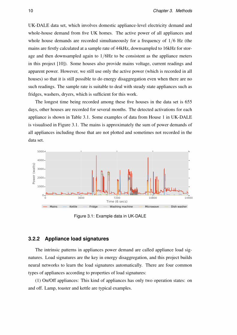
The longest time being recorded among these five houses in the data set is 655

days, other houses are recorded for several months. The detected activations for each

appliance is shown in Table 3.1. Some examples of data from House 1 in UK-DALE

is visualised in Figure 3.1. The mains is approximately the sum of power demands of

all appliances including those that are not plotted and sometimes not recorded in the

data set.

0 3600 7200 10800 14400

Time (6 secs)

0

1000

2000

3000

4000

5000

Pow

er

(watt

s)

Mains Kettle Fridge Washing machine Microwave Dish washer

Figure 3.1: Example data in UK-DALE

3.2.2 Appliance load signatures

The intrinsic patterns in appliances power demand are called appliance load sig-

natures. Load signatures are the key in energy disaggregation, and this project builds

neural networks to learn the load signatures automatically. There are four common

types of appliances according to properties of load signatures:

(1) On/Off appliances: This kind of appliances has only two operation states: on

and off. Lamp, toaster and kettle are typical examples.

3.2. Data 11

(2) Multi-state appliances: Multi-state appliances have a finite number of operating

states, they are also known as Finite State Machines (FSM), such as washing machine

and stove burner. These appliances often have repeatable switching pattern, which is a

distinctive pattern and useful for appliance identification.

(3) Continuously Variable Devices: The variable power draw characteristics of

continuously Variable Devices (CVD) have no fixed number of states. Power drill and

dimmer lights belong to this category. Lack of repeatability in power draw character-

istics, these type of appliances are hard to detect with traditional NILM approaches.

(4) Permanent consumer devices: These appliances work for a long duration such

as days or weeks and often consume a constant rate of energy, which are also called

’vampire appliances’. Smoke detector, alarms and telephone sets are typical examples.

The appliances from the 5 houses are different, they have different power demand

properties, Figure 3.2 shows the power demand histograms from house 1, 2 and 5. As

number of activations from these houses are very different, the y axis (number) is not

labelled, the figure shows the differences in the distribution of the appliances vary from

house to house. For example, the kettle from House 1 has lower active powers than

kettles from House 2 and 3.

2000 2400 2800 3200

0

2000

4000

6000

8000

10000

12000

14000

16000

18000

House

1

Kettle

2000 2400 2800 3200

0

500

1000

1500

2000

2500

3000

3500

4000

House

2

2000 2400 2800 32000

200

400

600

800

1000

House

5

60 80 100 120

0

100000

200000

300000

400000

500000

600000

Fridge

60 80 100 120

0

10000

20000

30000

40000

50000

60000

60 80 100 120

Power(watts)

0

20000

40000

60000

80000

100000

120000

140000

160000

180000

800 1200 1600 2000

0

5000

10000

15000

20000

25000

30000

35000

Microwave

800 1200 1600 2000

0

1000

2000

3000

4000

5000

6000

7000

8000

9000

800 1200 1600 20000

100

200

300

400

500

600

700

800

900

Figure 3.2: Histograms of power demands for appliances in different houses

3.2.3 Choice of appliances

Five appliances are investigated in the project: kettle, fridge, washing machine,

microwave and dish washer. Each of the appliances can be found in at at least three


houses in UK-DALE, which means the data of appliance is able to cover some varia-

tions within the same type, and will have better generalisation ability for deep learning.

Also, these five appliances have different complexity of load signatures and different

lengths in working duration. For example, kettles have simple on and off signatures

and work for about 4 minutes, while washing machine has complex patterns and of-

ten work for over 2.5 hours. These five appliances cover both simple and complex

appliances to test the performance of networks. Also, these appliances take up most

of the power consumption in UK-DALE data set [10], which meets the motivation of

this project. This means the disaggregation results of these five appliances will also be

very meaningful for consumption reduction.

3.3 Preprocessing and window extraction

3.3.1 Generating window samples

Before fed into the neural networks, the data should be transformed into consistent

input formats. Each sample is a 1×N vector, the data should be segmented into vec-

tors of constant widths, which are also called windows. As mentioned in section 1.2,

different networks will be trained for different appliances, while appropriate window

widths differ from appliance to appliance. In this work, the window width is chosen

the same as [11], see Table 3.4.

A most intuitive way to generate window samples is to slide windows across a

sufficient duration. This method, however, would cost too much storage space, espe-

cially for long window appliances. Also, most of the data would contain little useful

information as the appliances do not work most of the time. To maximise the infor-

mation included in data with limited storage space, we extract positive and negative

samples from the data set. As the disaggregation algorithm is supposed to work well

when appliances are and are not working, the data used for training and test must con-

tain both of the situations. More importantly, the disaggregation should perform well

when multi-state appliances are working at different states or modes. For example,

microwaves may have different power consumption patterns where they are set to dif-

ferent cook power, washing machines often have more than one modes: spin, heat,

dry, etc. There are also some appliances with simple working patterns, such as ket-

tles. The training data must include possible situations as many as possible, so that the

trained network will be able to perform good on different conditions. All these samples

3.3. Preprocessing and window extraction 13

Table 3.1: Number of activations per house

House 1 2 3 4 5

Kettle 3131 789 84 766 195

Fridge 17427 3448 0 4827 2986

Washing m. 560 50 0 0 112

Microwave 3562 384 0 0 66

Dish washer 211 91 0 0 47

that include activations are called positive samples. Positive samples are generated by

randomly place an activation within the window, with the constraints that: 1. the ac-

tivation must be completely included in the window; 2. there is no other activation

with in the window (the second constraint does not apply to fridges, as they are often

turned on and off very frequently). As seen in Table 3.1, the number of real activations

is not enough for neural networks. In these cases, each activation is duplicated. The

number of duplication is decide by making sure that enough 3.3 samples have been

generated. Duplication of activations solved two problems: 1. too few real activa-

tions; 2. activation in random positions for generalisation. However, it also caused

problems, which will be discussed in section 4.2. The activations are obtained using

Electric.get actiations() method in NILMTK toolkit. The parameters passed

to this method are shown in Table 3.2. These parameters also reveal some intrinsic

properties (like power range, working duration, etc) for these appliances.

We should not forget about situations that the target appliances are not working

within the windows. When the target appliance is not working, the network should

predict the power demand curve to be close to the time axis (power = 0), even if there

are other ’distractor’ appliances working. Samples that satisfy the conditions are called

negative samples. In practise, negative samples are generated by choosing a window at

a random period of time (same as the window width), this would occasionally includes

some positive samples, thus a second check is carried out and if the samples contain

any activation, they are rejected.

In short, both positive samples and negative samples should be included into the

training, validation and test set. The network should be trained at all possible states

of the target appliances, be able to distinguish between appliances with similar load

signatures, and correctly predict the power demand curve no matter whether the targets

are active or not.


Table 3.2: Parameters used to obtain activations

Appliance

On power

threshold

(watts)

Min. on

duration

(secs)

Min. off

duration

(secs)

Kettle 2000 12 0

Fridge 50 60 12

Washing m. 20 1800 160

Microwave 200 12 30

Dish washer 100 1800 1800

3.3.2 Synthetic data

It is a common practise in deep learning to artificially add some ’fake’ samples with

noise and reasonable changes to true data. This will help networks to be more robust

to noise and improve the generalization ability. For example, in hand-written digits

recognition, pepper and salt masking, Gaussian noise, slight rotation and translation

can be added to original digit images to generate synthetic data. This is also called

’data augmentation’.

In real applications, it would be quite often that some malfunctions or glitches

may happen to the sensors, which could cause noise, spikes or missing data. On the

other hand, it would be very likely that new combinations of appliances may occur,

but they are not included in the data set. For example, suppose people in the data set

like to boil water while using microwave to prepare food, thus the network trained by

this data is very competent in recovering kettle’s power from microwaves and other

appliances. However, if the trained network is used for another house where people

often drink hot water after they finish their lunch and turn on the dish washer. The

network may not perform so well as it has never encountered such situations before.

So, adding synthetic data to the training set would help the networks to improve their

performance on unseen situations.

Fortunately, it is very easy to generate synthetic data in this project. Arbitrarily

large number of synthetic samples can be generated by randomly combining appliance

specific data to be the fake ’mains’, while keeping the target appliance ground truths

as they are. As described in the last section, the balance of positive and negative

samples also needs to hold, 50% of the synthetic data is positive and 50% is negative.

The details of the algorithm is shown in Algorithm 1, which comes from [11]. The

3.3. Preprocessing and window extraction 15

synthetic data generator is implemented by my partner Chaoyun.

Algorithm 1 Generate synthetic data1: Inputs:

number of synthetic data needed, time-aligned mains readings y,

target submeter readings st and other four submeter readings

si, i = 1..42: while not enough synthetic data generated do3: Initialize the inputs and out puts to be zero vectors

4: Adds a positive sample from st to both inputs and out puts with 50% probabil-

ity

5: for every other appliance do6: Adds a positive sample from si to inputs with 25% probability

7: end for8: Save this sample, inputs is synthetic mains and out puts is synthetic ground

truth

9: end while

3.3.3 Training, validation and test set

After the positive, negative and synthetic samples have been generated, we can pre-

pare the data for neural networks. Neural networks need plenty of training samples to

be fine tuned, and a test set to evaluate the results. Also, there are numerous hyper pa-

rameters in neural networks that may have great impact on the actual performance. As

a result, it is helpful to track the learning process and prevent over fitting by evaluating

the networks on another separate test set after each epoch. This is called validation set.

Training, validation and test set should be carefully prepared in order for better

training and more accurate evaluation. Training set is one of the most important part

in deep learning, a good training data and a simple learning algorithm can often out-

perform a sophisticated algorithm [16]. The training set should cover most of the

situations that may appear in the test set, so that the parameters in the networks will

have been tuned by all possible conditions when evaluated. On the other hand, as

the squared error is used as the cost function, the proportions of positive and negative

samples should be carefully balanced. The training set needs to cover not only both

positive and negative samples, but also different usage patterns for some multi-state

appliances. Validation and test set serve similar purposes, so the sizes and propor-


Table 3.3: Number of samples used in training, validation and test set

Train/Val/Test Positive(×104) Negative(×104) Synthetic(×104) Total(×104)

Kettle 28/ 7/ 7 7/ 7/ 7 35/ 0/ 0 70/ 14/ 14

Fridge 12/ 6/ 6 8/ 2/ 2 20/ 0/ 0 40/ 8/ 8

Washing m. 8/ 2/ 2 2/ 2/ 2 10/ 0/ 0 20/ 4/ 4

Microwave 24/ 6/ 6 6/ 6/ 6 30/ 0/ 0 60/ 12/ 12

Dish washer 7.2/ 1.9/ 1.9 1.9/ 1.9/ 1.9 10/ 0/ 0 20/ 3.8/ 3.8

tions are the same to each other. As mentioned before, synthetic data is added into the

training set to improve generalisation, while these data are not real, thus they are not

included in validation and test set. The percentage of positive/negative/synthetic data

in the training, validation and test set are as follows:

Training set: 40% positive + 10% negative + 25% positive synthetic + 25% negative

synthetic

Validation set: 50% positive + 50% negative

Test set: 50% positive + 50% negative

That is to say, 65% of the training data contains activations (40%+ 25%), and 35%

doesn’t(10%+ 25%). And the performance is tested and validated on 50% positive

and 50% negative samples. Note that fridge works very frequently than other appli-

ances, so the proportion is adjusted (see Table 3.3).

The size of training/validation/test set and number of samples from positive, nega-

tive and synthetic data are shown in Table 3.3.

The data could also be generated by sliding the window across a very long time. In

this case the data would be much more similar to the real situations. However, there

would be too many samples that does not contain activations and the samples would

be very redundant, which may hurt the networks training. This may encourage the

networks fitting negative samples, and the networks would still have very low cost even

they predicts no activation because how few they are. Also, limited by computation

and storage resources, abundant information must be included in a relatively small-size

data.

3.4. Deep learning basics 17

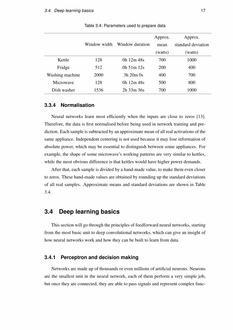
Table 3.4: Parameters used to prepare data

Window width Window duration

Approx.

mean

(watts)

Approx.

standard deviation

(watts)

Kettle 128 0h 12m 48s 700 1000

Fridge 512 0h 51m 12s 200 400

Washing machine 2000 3h 20m 0s 400 700

Microwave 128 0h 12m 48s 500 800

Dish washer 1536 2h 33m 36s 700 1000

3.3.4 Normalisation

Neural networks learn most efficiently when the inputs are close to zeros [13].

Therefore, the data is first normalised before being used in network training and pre-

diction. Each sample is subtracted by an approximate mean of all real activations of the

same appliance. Independent centering is not used because it may lose information of

absolute power, which may be essential to distinguish between some appliances. For

example, the shape of some microwave’s working patterns are very similar to kettles,

while the most obvious difference is that kettles would have higher power demands.

After that, each sample is divided by a hand-made value, to make them even closer

to zeros. These hand-made values are obtained by rounding up the standard deviations

of all real samples. Approximate means and standard deviations are shown in Table

3.4.

3.4 Deep learning basics

This section will go through the principles of feedforward neural networks, starting

from the most basic unit to deep convolutional networks, which can give an insight of

how neural networks work and how they can be built to learn from data.

3.4.1 Perceptron and decision making

Networks are made up of thousands or even millions of artificial neurons. Neurons

are the smallest unit in the neural network, each of them perform a very simple job,

but once they are connected, they are able to pass signals and represent complex func-


tions. Inspired by Warren McCulloch and Walter Pitts[14], perceptron was developed

in 1950s, by Frank Rosenblatt. Perceptrons are very similar to the most commonly-

used neurons today: sigmoid neurons. Before going there, we are going to give some

explanations on how perceptrons work.

Output

Figure 3.3: The sturcuture of a perceptron

What perceptrons do is simple: each perceptron takes several inputs, and each input

has a corresponding weight. The perceptron sums them up according to their weights

and emit 1 if the sum is greater than a threshold, and emit 0 if not. The threshold is

called ’bias’, and the operation is similar to a step function (except for values at 0).

Figure 3.3 shows a typical structure of perceptron.

Perceptron could also be written as a function:

output =

{1, if ∑i xiwi > threshold

0, if ∑i xiwi ≤ threshold(3.1)

Here is a simple example to illustrate how perceptrons gather all evidence and make

decisions/predictions based on that. Suppose some of your friend likes music, some

day he passed by a CD shop and saw a new-arrival album. Assuming we are only

considering two factors regarding if he would buy that album: 1. if the price is high

2. if the album interest him. These factors can be denoted by two binary variables x1

and x2. For example, if the price is high, then x1 = 1, x1 = 0 if not. Similarly, x2 = 1

he the album interest him, x2 = 0 otherwise. Suppose your friend would only buy it

only if he likes it and the price isn’t high. Then his behaviour can be represented by a

perceptron with w1 = 1,w2 =−1, and threshold = 0. And now this perceptron is able

to make decisions or predictions for your friend on other all possible situations.

This example can be extended further: it would be possible to adjust the decision-

making behaviour by changing the weights and the bias. if your friend has a well-paid

job, and he would buy the album as long as it interests him, no matter how much it is.

Then the weight can be adjusted to w1 = 2,w2 =−1, and threshold = 0, and now the


perceptron is perfectly adjusted to the new situations.

Actually, tuning networks by changing weights and bias is exactly how the net-

works are trained to learn.

3.4.2 Sigmoid neurons

Gradient descent training initialises the parameters at some point in the high-dimensional

weight space, and then they are adjusted a little bit evry time to improve the outputs

gradually. Perceptrons, however, can flip the outputs for very tiny changes in param-

eters due to its unsmoothness at 0. Therefore, another type of neurons is needed:

sigmoid neuron.

Sigmoid neurons were the most widely used neurons, the only difference between

sigmoid neurons and perceptrons is the activation function: sigmoid neurons take sig-

moid function rather than step function. Sigmoid function is defined as equation 3.2:

σ(x)≡ 11+ e−x (3.2)

Taking weights and bias into account, a sigmoid neuron can be written as :

11+ exp(−(∑i wixi +b))

(3.3)

Sigmoid neurons have some useful properties: sigmoid functions are monotonously

increasing functions, they can project any unbounded real values into (0, 1), which is

very suitable to represent probabilities. Also, derivation of sigmoid function can be

easily computed: ∇σ(x) = σ(x)(1−σ(x)).

However, the outputs of regression tasks are often not restricted in (0,1). Therefore,

the activation functions of the output layer are often set as linear in regression tasks.

Linear neurons emit the values as it takes in, which means the neurons output ∑i wixi+

b.

3.4.3 Multilayer perceptron

A simple example in section 3.4.1 has been given to illustrate how perceptrons

work. However, more complex architectures are needed for more complex tasks. Fig-

ure 3.4 is an example of multilayer perceptrons (MLP). Perceptrons are grouped into

’layers’, and they are connected to higher layers by feeding their outputs into higher

layers as inputs. The layer at the bottom is called input layer, it takes in feature vectors


and allocate them to the first hidden layer. A hidden layer means it is not a input layer

nor an output layer. The output layer emits the results we want, it outputs probabilities

in classification tasks, and outputs real values for regression tasks. Unlike the name,

artificial neurons in the MLPs are often not perceptrons. They can take different types

of activation functions, such as linear, sigmoid, ReLU and tanh. Different types of

activation functions has different learning properties and representation power.

Complex networks often have more representation power, and can extract complex

structures and features from the data. In image classification tasks, for example, deep

networks are built and achieved better results than hand-crafted feature recognition per-

formance [12]. In image classification, the first hidden layer is assumed to learn very

basic features like edges, grey scale values, deeper layers may learn structures, patterns

and other high level features, and is finally the networks are able to ’understand’ the

data in a high conscious level.

3.4.4 Cost function and optimization

3.4.4.1 cost function

Networks start learning by trying to ’fit’ the training set as much as possible.

A learning algorithm helps the networks perform better each time by making small

changes to the weights and biases. Every time the parameters of the network can be

tuned a little bit closer to our expected outcomes, and this process is done by optimis-

ing a ’cost function’. This section will describe what cost functions are and how to

optimise them.

A cost function E, sometimes also called ’error function’ or ’loss function’, mea-

sures how far the predicted outcomes are from the expected results. Euclidean dis-

tance, which is also called squared error function, is typically used in regression. As

this project is a regression tasks, Euclidean distance is used to measure how close the

prediction is to the ground truth.

However, cost function is often not the metrics that will be used to evaluate the

final performance. For example, hand-written digits recognition uses cross entropy as

its cost function, while accuracy is used to evaluate. In this project, squared error is

used for cost function, as the networks are designed to predict the same energy demand

as close as possible, but the metrics used are F1 score, mean absolute error, etc. The

metrics used will be discussed in later section. The reason why the metrics can not

be used as cost function is: the metric functions regarding network parameters are not


smooth and sometimes impossible to derive, which would make the training inefficient

or even impossible.

3.4.4.2 optimisation

Now there is a cost function E that the networks want to minimize, the methods

used is gradient descent training. What gradient descent training does is by repeatedly

moving a small distance down the weight space in the direction which the cost function

E decreases most rapidly. The process of gradient descent is shown bellow.

Algorithm 2 Gradient descent learning1: Inputs:

training set T , k×d weight matrix W , learning rate lr

2: Initialize:Initialize the weight matrix W with small random values

3: while not converge do4: for every training sample n do5: Compute the error En

6: Compute the gradients ∂E∂Wk,d

for all k×d parameters

7: Update the total gradient by a small step of lr: W ←W −η∂E∂W , for all k,d

8: end for9: end while

Algorithm 2 is batch gradient descent, which means every training data is passed

through in every epoch. This would cost a lot of time when the training set is large,

while stochastic gradient descent (SGD) gives a solution. Instead of summing up gradi-

ents for all training samples, SGD approximates the gradient ∂E∂W with a single sample

∂En∂W , this is very suitable for very large data set. However, SGD estimation can be

quite noisy as it uses single gradient to estimate overall gradients. What we use in our

project is minibatch learning, which is a intermediate between batch learning and SGD.

Minibatch learning can also be computationally efficient when applying vectorisation

to training samples. Also, minibatch learning can possibly have smoother estimation

than SGD. This project used 1000 for training minibatch size, and 5000 for test and

validation batch size. Large batch sizes cost less time but more memory usage, the

batch sizes were chosen as a trade off between memory and time.

Different learning rates and learning schedulers also have a great impact on the

outcomes. Large learning rates reduce the epochs needed to get close to the local


minimum, they also help to jump over shallow valleys. However, large learning rates

may cause instability, updating the parameters to unreasonable and extreme values,

also, large learning rates may cause the parameters swing around the local minimum,

and is very difficult to get lower. A compromise is introducing momentum, which

means the parameters are likely to move in the same direction as last epoch (Equation

3.4).

∇E(Wt) = β∇E(Wt−1)+(1−β)η∂E∂W

(Wt−1) (3.4)

Wt is the weight matrix at epoch t, and ∇E(Wt) means the gradient of cost func-

tion E regarding weight matrix Wt . β is a coefficient to control the momentum, is has

range (0,1), the larger it is, the more will the weights be upgraded to the similar di-

rection as the last epoch. η is the learning rate. In this project, nesterov momentum

learning scheduler is used, the momentum β is set to 0.9. Learning rate η is set to 0.1.

Nesterov momentum is an improved version of traditional momentum scheduler. The

difference between nesterov momentum and traditional momentum is the update for

velocity (second term of the right hand side of Equation 3.4). Nesterov momentum

can be described as Equation 3.5.

∇E(Wt) = β∇E(Wt−1)+(1−β)η∂E∂W

(Wt−1 +β∇E(Wt−1)) (3.5)

The basic idea behind nesterov momentum is: instead of upgrading the parameters

directly, it firstly ’attempts’ to upgrade the parameters with momentum β∇E(Wt−1),

secondly, the a bias is estimated by the gradients at the attempts, at last, the param-

eters are upgraded by completing these two stages. Nesterov momentum has better

convergence rate O(1/T 2) than classical momentum (O(1/T )) in smooth convex op-

timisation, and it can still keeps the learning step relatively consistent, which makes

it easier for comparisons. This is the reason why nesterov momentum is used in the

project.

3.4.5 Forward and backward propagation

For single layer networks, the parameters can be trained directly and intuitively.

However, training becomes more complex when the networks have multiple layers:

hidden units also affect the final results by their outputs, but their error (cost) can not

be computed directly. Therefore, an efficient learning algorithm is needed: backprop-

agation of error.

3.5. Convolutional neural networks 23

The backpropagation algorithm is just the chain rule of taking derivatives. In order

to measure the error of every layer, a forward propagation is carried out, as the chain

rule starts from the output layer. The error can be passed through higher layer to lower

layer, which makes computing gradient possible. Using root mean squared error cost

as an example, the process can be described in Figure 3.4.

Inputs x

Outputs y

Forward

propagation

Backward

propagation

Parameter

updates

Network

model

Figure 3.4: Illustration of forward and backward propagation

Figure 3.4 shows a network with three layers, but the propagation algorithm can be

easily extended to networks with any number of layers. To summarize, the backprop-

agation algorithm can be described as the following steps:

1. Pick an input vector x from the training set and forward propagate to calculate the

output vector y;

2. Compute the error En using target vector t

3. Obtain error signals δ(l) for each output unit

4. Obtain error signals δ(l−1) for each hidden unit with back propagation

5. Go through all training samples or one minibatch to sum up the derivatives

3.5 Convolutional neural networks

Convolutional neural networks have been successfully applied in many areas like

image classification [12], face recognition [23] and action recognition [21]. They pro-

vide good solutions for parameters reduction and have great performance in many

tasks.


All layers in multilayer perceptrons are fully connected, which ignore the structure

information. This would often connect two irrelevant features together due to ’occa-

sional’ correlations. Also, it would be hard for MLP to learn a same local feature across

the whole feature vectors, such as edges in images, activations in power demands, etc.

Convolutional neural networks (CNN) can do much better in this case.

These problems are dealt with in three aspects in CNN: 1. local receptive fields; 2.

weight sharing; 3. pooling. All these aspects help to reduce the number of parameters

while still makes the learning efficient as local features can be most useful than some

random features being connected.

Unlike fully connected layers, each convolutional hidden unit is connected to only

a region of features from previous layer, which is called local receptive field. This

allows the detection of a same local feature across the whole input. The stride is

chosen as 1 in this project to fully utilise the inputs. Therefore, for an n length and a

m size kernel (another name of local receptive field), the output hidden layer will be

of length n−m+1. In this project, the convolutional operation is in 1D, for tasks like

image recognition, the convolutional will be 2D. All the kernel shared same weights,

and its feature extraction over all parts of input is the same. The extracted features are

called feature map, which encodes the translation invariance, meaning it could detect

features no matter where the appliance activation is within the window. In practise,

there is often more than one feature maps for different types of features extracted to

be used for later layers. Pooling helps to compress information from previous layers,

reduce number of parameters even further. However, pooling layer is not used in this

project, as [11] found that pooling layer has little effect on the performance.

The convolutional hidden unit equation can be written as Equation 3.6 (suppose the

activation function is sigmoid):

hi = sigmoid(m

∑k=1

wkxi+k +b) (3.6)

This can be written as an convolutional operation ∗ in Equation 3.7:

h = sigmoid(w∗ x+b) (3.7)

In backpropagatin of convolutional neural networks, the region of hidden unit con-

nected to each input unit should be considered. As described in section 3.4.5, the error

δ needs to be considered (see Equation 3.8):

3.6. Stacked denoising autoencoders 25

……

Local receptive fields

kernel size = 5stride = 1

Input layer 15 units

Hidden layer11 units

Figure 3.5: Forward propagation of convolutional neural networks

δns = ∑

j∈connected to sw jsδ

n+1j f ′(as) (3.8)

For a m length kernel, the feature map is padded with (m−1) length of zeros both

left and right. After that, the back propagation can be carried out as another convolution

by applying the rotated weight matrix (by 180 degree) across the padded feature map

(Figure 3.6).

Input/Pooling layer

Convolutional layer

Connected units

Figure 3.6: Backpropagation of convolutional neural networks

3.6 Stacked denoising autoencoders

Stacked denoising autoencoders (SdA), which try to ’recover’ the inputs from a

corrupted version, have shown significantly better performance in image classification

than single hidden layer autoencoders due to its nonlinearity [24]. Stacked denoising

autoencoders are also used in unsupervised pretraining, which helps to initialise deep


networks for better convergence. This project builds a SdA for the first purpose: the

inputs (mains), can be seen as a noisy activation, where the noise refers to all appli-

ances except the target. SdA is expected to learn useful representation of the input,

and recover the target activation from that. The structure of SdAs used in this project

is shown in Figure ??. There is some symmetry in the structures, as the inputs are

passed through a 1D convolutional layer to extract simple local features such as sud-

den increase and decrease in power demand. After that, the outputs are passed through

two fully connected layers and mapped to the same length (input window width) as the

inputs. These layers can be seen as an encoder, which projects the original input non-

linearly to another feature space. The later layers are the decoder part, which passed

through symmetric fully connected layers and a ’deconvolutional’ layer (despite the

name, this layer is actually another convolutional layer). After that, they results are

combined and projected to the uncorrupted version of the inputs: the predicted power

demand of a target appliance.

The network structure for SdAs used in the project is shown below:

1. Input (window width depends on target appliance)

2. 1D conv (filter size=4, stride=1, number of filters=8, activation functions = linear,

border mode=valid)

3. Fully connected (N=(window width-3) × 8, activation function=ReLU)

4. Fully connected (N=window width, activation function=ReLU)


5. 1D cov (filter size=4, stride=1, number of filters=1, activation functions = linear,

border mode=valid)



8. Output (N=window width, activation function=Linear)

For some washing machine networks, the layer 3 and 6 are shrunk to N=(window

width-3) × 4 to be able to fit into the memory.

3.7 Long short term memory

Recurrent neural networks (RNN) are especially useful in dealing with sequential

data, and are able to learn context information very well. However, traditional RNNs

suffer from the vanishing gradients problem, which causes the network hard to learn

3.7. Long short term memory 27

Input layer

1×1×window

1D conv

8×1×(window-3)

4

Dense encoder & decoder layers

(window-3)×4; window; (window-3)×4

Encoder Decoder

1D conv

8×1×(window-3)

Output layer

1×windowDense layer

window×2

Figure 3.7: Network architecture of convolutional stacked denoising autoencoders

long term memory. Long short term memory (LSTM) is a special type of recurrent

neural networks, and is able to overcome this problem by learning ’state’ for the long

term event, so that it is able to correlate events for a long period of time. What’s

more, LSTM is able to learn how long it requires to get sufficient information, and

only consider short or long term context depends on the situations [5].

The LSTM layer (also called block) is made up of several parts: input gates, forget

gates, cells and output gates (Figure 3.8). The functions of these parts are described in

Equation 3.9 to 3.17, which also explain the forward propagation.

Input gates:

atl =

I

∑i=1

wi,lxti +

C

∑c=1

wc,lst−1c +

H

∑h=1

wh,lbt−1h (3.9)

btl = f (at

l) (3.10)

Input gates in Equation 3.9 and 3.10 calculate the weighted sum of all inputs xi for

this LSTM block, where the bh represented the connection between cells. sc is called

peephole connection, reading information from the cell.

Forget gates:

atφ =

I

∑i=1

wi,φxti +

H

∑h=1

wh,φbt−1h +

C

∑c=1

wc,φst−1c (3.11)

btφ = f (at

φ) (3.12)

Forget gates in Equation 3.11 and 3.12 take similar format as the input gates, but

they serve the purpose to reduce unnecessary context information.

Cells:

atc =

I

∑i=1

wi,cxtt +

H

∑h=1

wh,cbt−1h (3.13)

stc = bt

φst−1c +bt

lg(atc) (3.14)


Input gate

Forget gate Output gate

Cell

LSTM

blockf

g

f f

h

Figure 3.8: Structure of a LSTM block

Cells (Equations 3.13 and 3.14) are the core parts in LSTMs, they are controlled

by forget gates to record the states as compact representations for signals passed from

the past and the future (for bidirectional LSTMs).

Output Gates:

atw =

I

∑i=1

wi,wxti +

H

∑h=1

wh,wbt−1h +

C

∑c=1

wc,wstc (3.15)

btw = f (at

w) (3.16)

Cell outputs:

btc = bt

wh(stc) (3.17)

The block outputs values using the combinations of cell states and results from the

output gates.

The backward propagation for LSTM is described in Equation 3.18 to 3.24:

εtc ≡

∂L∂bt

cε

ts ≡

∂L∂st

c(3.18)

Cell outputs:

εtc =

K

∑k=1

wc,kδlk +

G

∑g=1

wc,gδl+1g (3.19)

3.8. Energy disaggregation 29

Output gates:

δtw = f ′(at

w)C

∑c=1

h(stc)ε

tc (3.20)

States:

εts = bt

wh′(stc)ε

tc +bt+1

φε

t+1s +wc,lδ

t+1l +wc,φδ

t+1φ

+wc,wδtw (3.21)

Cells:

δtc = bt

lg′(at

c)εts (3.22)

Forget gates:

δtφ = f ′(at

φ)C

∑c=1

st−1c ε

ts (3.23)

Input gates:

δtl = f ′(at

l)C

∑c=1

g(atc)ε

ts (3.24)

The network architecture for LSTM used in the project is shown below:

1. Input (window width depends on target appliance)

2. 1D conv (filter size=4, stride=1, number of filters=16, activation functions = linear,

border mode=valid)

3. LSTM (N = window width, bidirectional)

4. LSTM (N = window width × 2, bidirectional)

5. Fully connected (N = window width × 4, activation function=Sigmoid)

6. Output (N = window width, activation function=Linear)

The LSTM networks are trained by my partener, Chaoyun Zhang.

3.8 Energy disaggregation

Once the networks have been trained, they can be used to disaggregate mains se-

quence of arbitrary length that longer than 3 hours with sample rate of 1/6Hz (the

longest window duration). We can slide windows through the whole sequence and

forward propagate them through their networks, with the stride equal to their window

width (the reason why the stride is picked will be discussed in section ??). Start and

the end of the input sequence are padded with same values as the edges if its length

can not be divided evenly by the window width. Therefore, the predicted results for

each appliance can be obtained by connecting the outputs returned by networks since

there is no prediction overlapping.


Mains readings (1/6 Hz)

... ...

Slide

windows

...Net

1

Net

2

Net

3

...

App1

...

App2

App3

Stride = window

width

Pad start and end

Predict1

Predict2

Predict3

Predicted readings (1/6 Hz)

Figure 3.9: Network structures of convolutional stacked denoising autoencoders

3.9 Optimisation

Paper [11] developed an end-to-end approach for energy disaggregation. However,

the networks can not always give reasonable predictions due to limited training re-

sources and the limitation of network representation power, while these problems do

not have a quick solution. Inspired by [25], further optimizations can be carried out

on the predicted outputs of neural networks. The energy disaggregation optimizations

could help to tune the outcomes to be more reasonable. Three different optimisations

were carried out in this project. Optimization 1 is described as bellow:

min{xi}Ii=1 ∑

i,t(xi,t− zi,t)

2

subject to:

∑i

xi,t <= yt , t = 1, ...,T

yt is the actual mains readings, xi,t denotes the power demand of ith appliance at

time t. ut means all power demands from unknown appliances. zi,t is the predictions

from the trained networks, which try to estimate the power demand xi,t of ith appliance

3.9. Optimisation 31

at time t. In the optimisation, it is constrainted that the sum of estimated power de-

mands is no greater than the actual mains readings. Also, the predicted power should

be non-negative.

Optimisation 1 tries to minimise the overall matching error between optimisation

and neural network predictions for a period of time, and will shift unreasonable pre-

dictions somewhere else. A more reasonable approach is optimisation 2, which only

adjust predictions within the same time. This is equivalent to optimisation 1 being

carried out for every time point. Optimisation 2 is shown bellow:

∀ t, min{xi}Ii=1 ∑

i(xi,t− zi,t)

2

subject to:

∑i

xi,t <= yt , t = 1, ...,T

Optimisation 3 is very similar to optimisation 2, which adds an additional nor-

malisation constant Ni for each appliance. Ni is chosen by the on power threshold of

target appliance (see Table 3.2). This would prevent the optimisation from focusing

only on high power demand appliances and shifting their error to low power demand

appliances. Optimisation 3 can be written as:

∀ t, min{xi}Ii=1 ∑

i

(xi,t− zi,t)2

Ni

subject to:

∑i

xi,t <= yt , t = 1, ...,T

These optimisation tasks were solved with disciplined convex programming, which

is implemented with CVX package in MATLAB [4].

Chapter 4

Results and evaluation

4.1 Metrics

The following metrics will be used to evaluate the performance of these neural net-

works: F1 score, precision, accuracy, proportion of total energy correctly assigned and

mean absolute error. They are defined as follows:

Terms:TP: number of true positives

FP: number of false positives

FN: number of false negatives

P: number of positives in ground truth

N: number of negatives in ground truth

y(i)t : appliance i estimated power at time t

y(i)t : appliance i actual power at time t

Definitions:F1 = 2× precision×recall

precision×recall

precision = T PT P+FP

recall = T PT P+FN

accuracy = T P+T NP+N

mean absolute error = 1T ∑

Tt=1 |yt− yt |

These metrics can efficiently evaluate how good the energy disaggregation perform.

High recall rates mean the energy disaggregation algorithm would not miss not many

real activations, most of the true activations are recalled. High precision scores mean

33

34 Chapter 4. Results and evaluation

most of the returned activations are real, which means the predicted activations are

quite trustworthy. Accuracy measures how accurate the predicted outcomes are as a

whole. F1 score is a harmonic mean of precision and recall, it is able to reflect the

performance on both situations when appliance is and is not active. However, all these

metrics needs a threshold to determine if the target is ’active’. The threshold is chosen

as Table 3.2. The predicted results can be very sensitive to the thresholds, as it is often

the situation that network correctly detect a real activation, but the predicted curves are

not high enough to reach the threshold values. It is possible to adjust the thresholds

to get high scores. Therefore, mean absolute error is needed to provide another key

information: if the predicted power demands are close to the ground truth. It could

be the very important since whether the prediction is close to the ground truth directly

affects the estimates of power consumption in real applications. Also, these metrics

are widely used to evaluate energy disaggregation algorithm. Measuring them makes

it easy to compare the work with other relevant work.

4.2 Disaggregation results

To find out how different types of networks perform and how synthetic data in-

fluences the disaggregation results, five networks are trained and evaluated for each

appliance: 1. SdAs (the architectures are described in section 3.6) on full training set;

2. SdAs on real-data training set (excluding synthetic data); 3. LSTMs on full training

set; 4. LSTMs on real-data training set; 5. multilayer perceptron on full training data.

Therefore there are 25 networks in total to be compared and analysed. The results of

LSTM networks are from my partner, Chaoyun.

The performance using the metrics in 4.1 is shown in Figure 4.1.

As shown in the plot, the networks perform generally very good on test situations

that have been fully trained. This means the networks are tested on houses have been

seen during training. MLPs can perform almost equally well as other complex net-

works in simple load signatures appliances such as kettle and fridge. However, when

appliances have several working mode or patterns like microwave and dish washer,

SdAs and LSTMs will outperform MLPs. The washing machine is an exception.

Washing machine networks are the largest ones among all appliances due to its long

window (2000). Large amount of trainable parameters need a large training set to be

well tuned. The number of training samples used in this project are far from enough.

Although the test set, network structures and training epochs are all different, but a

4.2. Disaggregation results 35

0 1 2 3 4 5

0

0.5

1

F1score 0.

900.

930.

940.

930.

93

Kettle

0 1 2 3 4 5

0

0.5

1

Precisionscore 0.

990.

990.

990.

990.

99

0 1 2 3 4 5

0

0.5

1

Recallscore 0.

820.

880.

890.

870.

89

0 1 2 3 4 5

0

0.5

1

Accuracyscore 0.

980.

990.

990.

980.

99

0 1 2 3 4 5

0

100

200Meanabsolute

error(watts) 59

.446

.346

.247

.446

.9

0 1 2 3 4 5

0.0

0.2

0.4

0.6

0.8

1.0

0.83

0.86

0.84

0.80

0.64

Fridge

0 1 2 3 4 5

0.0

0.2

0.4

0.6

0.8

1.0

0.86

0.88

0.90

0.84

0.52

0 1 2 3 4 5

0.0

0.2

0.4

0.6

0.8

1.0

0.80

0.84

0.78

0.77

0.82

0 1 2 3 4 5

0.0

0.2

0.4

0.6

0.8

1.0

0.90

0.91

0.91

0.88

0.72

0 1 2 3 4 5

0

50

100

150

200

16.8

14.7

16.3

18.3

35.5

0 1 2 3 4 5

0.0

0.2

0.4

0.6

0.8

1.0

0.59

0.61

0.61

0.35

0.35

Washingmachine

0 1 2 3 4 5

0.0

0.2

0.4

0.6

0.8

1.0

0.43

0.45

0.45

0.21

0.22

0 1 2 3 4 5

0.0

0.2

0.4

0.6

0.8

1.0

0.92

0.94

0.94

0.97

0.97

0 1 2 3 4 5

0.0

0.2

0.4

0.6

0.8

1.0

0.75

0.77

0.77

0.32

0.33

0 1 2 3 4 5

0

50

100

150

200

76.5

66.2

64.1

129.

134.

0 1 2 3 4 5

0.0

0.2

0.4

0.6

0.8

1.0

0.77

0.85

0.85

0.85

0.83

Microwave

0 1 2 3 4 5

0.0

0.2

0.4

0.6

0.8

1.0

0.64

0.74

0.75

0.76

0.73

0 1 2 3 4 5

0.0

0.2

0.4

0.6

0.8

1.0

0.98

0.98

0.98

0.97

0.98

0 1 2 3 4 5

0.0

0.2

0.4

0.6

0.8

1.0

0.96

0.97

0.97

0.98

0.97

0 1 2 3 4 5

0

50

100

150

200

62.7

44.6

46.5

43.8

47.1

0 1 2 3 4 5

0.0

0.2

0.4

0.6

0.8

1.0

0.65

0.73

0.66

0.73

0.72

Dishwasher

0 1 2 3 4 5

0.0

0.2

0.4

0.6

0.8

1.0

0.50

0.60

0.50

0.59

0.58

0 1 2 3 4 5

0.0

0.2

0.4

0.6

0.8

1.0

0.93

0.94

0.95

0.95

0.95

0 1 2 3 4 5

0.0

0.2

0.4

0.6

0.8

1.0

0.72

0.81

0.73

0.81

0.80

0 1 2 3 4 5

0

50

100

150

200

56.2

46.4

45.6

40.9

38.9

MLP SdA SdA (ns) LSTM LSTM (ns)

Figure 4.1: Performance evaluation of different networks

comparison with Kelly’s work [11] is still presented here (See Table 4.1) to show how

this work perform. As all these differences, comparing every metric for all networks

does not make too much sense, so only the networks with best scores are shown. The

best scores may come from different networks, the mean absolute error shown are the

minimum (best performance) of Kelly’s work.

All networks except LSTM(ns) fridge has better F1 score than Kelly’s result. How-

ever, due to the difference in test set, our work has much larger mean absolute error

than Kelly’s results. This is because the test set in this project is composed with only

Table 4.1: Kelly’s results

Kettle FridgeWashing

machineMicrowave

Dish

washer

F1 score 0.71 0.81 0.25 0.62 0.60

Precision score 1.00 0.83 0.15 0.50 0.45

Recall score 0.63 0.79 0.62 0.92 0.99

Accuracy score 1.00 0.85 0.76 0.99 0.95

Mean absolute error (watts) 16 25 28 13 21


50% negative samples, however, in real case, negative samples can take up to over

90%, and the mean absolute error will be low at negative samples. In short, the mean

absolute error in our work can not be directly compared with Kelly’s results, but the

F1 scores are much better.

Mean absolute error can be not compared between appliances, as the average power

varies from appliance to appliance. As the results show, long working time ,multiple

state, low power demand appliances are much harder to predict and detect, due to sev-

eral reasons: 1. these networks are too huge to be fine tuned in limited computation

resources; 2. complex and various working patterns, which makes training parame-

ters in networks much harder and ambiguous. 3. low power demand appliances can

be easily ignored when covered by other vampire appliances because they have little

distinguishable changes in power demands.

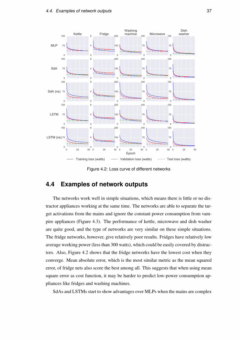
4.3 Convergence and loss

The networks are trained with a same learning scheduler: nesterov momentum

with 0.1 learning rate and 0.9 momentum. Therefore, the loss curve of training and

validation can be compared (Figure 4.2).

As shown in 4.2, validation loss would finally converge to the test loss. This satisfy

our expectation, which means the validation set successfully simulated the test set.

The learning is efficient as most blue curves drop very quickly, some networks even

begins to overfit very soon, such as fridge MLP and Washing mahchine MLP and SdA.

Actually, MLPs tend to be easier to overfit, as all its layers are fully connected, there

is a high probability that many redundant and occasional parameters will be learnt to

fit training set. However, convolutional layers and LSTMs could make better use of

parameters and the parameters are much easier to interpret than MLPs.

Another interesting phenomenon is: the training loss of training set that contains

no synthetic data (ns), would be significantly higher than validation loss. What’s more,

the gap between validation and test loss for non-synthetic networks are quite big. A

possible reason is the complexity of the data. As described in section ??, synthetic data

would be much easier to disaggregate than real data because there is fewer appliances

mixed together. This could be seen as some times the full data minibatch contains

some ’toy’ samples, which are easier to optimise, while all samples in non-synthetic

data set are complex real situations, which takes longer to optimise.

4.4. Examples of network outputs 37

0 10 20 30 40 50

0

75

150

MLP

Kettle

0 10 20 30 40 50

0

75

150

SdA

0 10 20 30 40 50

0

75

150

SdA (ns)

0 10 20 30 40 50

0

75

150

LSTM

0 25 500

75

150

LSTM (ns)

0 10 20 30 40 50

0

4

8Fridge

0 10 20 30 40 50

0

4

8

0 10 20 30 40 50

0

4

8

0 10 20 30 40 50

0

4

8

0 25 500

4

8

0 10 20 30 40 50

0

100

200

Washingmachine

0 10 20 30 40 50

0

100

200

0 10 20 30 40 50

0

100

200

0 10 20 30 40 50

0

100

200

0 25 50

Epoch

0

100

200

0 10 20 30 40 50

0

70

140Microwave

0 10 20 30 40 50

0

70

140

0 10 20 30 40 50

0

70

140

0 10 20 30 40 50

0

70

140

0 25 500

70

140

0 10 20 30 40 50

0

75

150

Dishwasher

0 10 20 30 40 50

0

75

150

0 10 20 30 40 50

0

75

150

0 10 20 30 40 50

0

75

150

0 25 500

75

150

Training loss (watts) Validation loss (watts) Test loss (watts)

Figure 4.2: Loss curve of different networks

4.4 Examples of network outputs

The networks work well in simple situations, which means there is little or no dis-

tractor appliances working at the same time. The networks are able to separate the tar-

get activations from the mains and ignore the constant power consumption from vam-

pire appliances (Figure 4.3). The performance of kettle, microwave and dish washer

are quite good, and the type of networks are very similar on these simple situations.

The fridge networks, however, give relatively poor results. Fridges have relatively low

average working power (less than 300 watts), which could be easily covered by distrac-

tors. Also, Figure 4.2 shows that the fridge networks have the lowest cost when they

converge. Mean absolute error, which is the most similar metric as the mean squared

error, of fridge nets also score the best among all. This suggests that when using mean

square error as cost function, it may be harder to predict low-power consumption ap-

pliances like fridges and washing machines.

SdAs and LSTMs start to show advantages over MLPs when the mains are complex


0 20 40 60 80 100 120

-1.0

1.5

4.0

Inpu

ts

Kettle

0 20 40 60 80 100 120

-1.0

0.5

2.0Ta

rget

s 0 100 200 300 400 500-0.6

-0.1

0.4Fridge

0 100 200 300 400 500

-0.6

-0.3

0.00 20 40 60 80 100 120

-1.0

2.0

5.0Microwave

0 20 40 60 80 100 120

-1.0

0.5

2.00 200 400 600 800 1000 1200 1400

-1.0

1.5

4.0Dish washer

0 200 400 600 800 1000 1200 1400

-1.0

1.5

4.0

0 20 40 60 80 100 120

1.0

0.5

2.0

MLP

0 20 40 60 80 100 120

1.0

0.5

2.0

SdA

0 20 40 60 80 100 120

1.0

0.5

2.0

SdA

(ns)

0 20 40 60 80 100 120

1.0

0.5

2.0

LSTM

0 64 1281.0

0.5

2.0

LSTM

(ns)

0 100 200 300 400 500

0.6

0.3

0.0

0 100 200 300 400 500

0.6

0.3

0.0

0 100 200 300 400 500

0.6

0.3

0.0

0 100 200 300 400 500

0.6

0.3

0.0

0 256 512

Window (number of samples)

0.6

0.3

0.0

0 20 40 60 80 100 120

1.0

0.5

2.0

0 20 40 60 80 100 120

1.0

0.5

2.0

0 20 40 60 80 100 120

1.0

0.5

2.0

0 20 40 60 80 100 120

1.0

0.5

2.0

0 64 1281.0

0.5

2.0

0 200 400 600 800 1000 1200 1400

1.0

1.5

4.0

0 200 400 600 800 1000 1200 1400

1.0

1.5

4.0

0 200 400 600 800 1000 1200 1400

1.0

1.5

4.0

0 200 400 600 800 1000 1200 1400

1.0

1.5

4.0

0 768 1536

1.0

1.5

4.0

Figure 4.3: Example disaggregation results of simple situations

and contains multiple appliances working simultaneously (Figure 4.4). The example

results clearly show that MLPs will predict some ’noise’ around the start and end of the

activations, and the shape of MLPs predicted results often have vague and ambiguous

edges. As the windows of LSTM networks already include most of the context, they

perform similar as the SdA networks.

As described in section 3.3.1, the training sets do not contain situations when the

activations are cut off: only a part of the activation is contained in the window. As a

result, the networks will predict very bad values when this happens. Figure 4.5 shows

that the predictions will change drastically when the networks can not find a rising

edge (see 3,4,5,6 subplots). As shown in the plot, the predicted activations tend to start

from zero, which does not apply to the cases where the real activation is cut off by left

edge of the window. This explain the reason why the disaggregation stride is equal

to the window width in section 3.8: when taking the mean of all predicted values, the

failed samples will lower the average and make the predicted results generally smaller

than the ground truth. In order to avoid this, the disaggregation windows should not

overlap. Although some activations will still be cut off between windows, but it still

shows much better results than directly taking means of overlapped predictions. This

kind of failure is the main reason that limits the results.

4.5. Optimisation results 39

0 20 40 60 80 100 120

-1.0

1.5

4.0

Inpu

ts

Kettle

0 20 40 60 80 100 120

-1.0

0.5

2.0

Targ

ets 0 100 200 300 400 500

-0.6

-0.1

0.4Fridge

0 100 200 300 400 500

-0.6

-0.4

-0.20 20 40 60 80 100 120

-1.0

2.0

5.0Microwave

0 20 40 60 80 100 120

-1.0

0.5

2.00 200 400 600 800 1000 1200 1400

-1.0

3.0

7.0Dish washer

0 200 400 600 800 1000 1200 1400

-1.0

1.5

4.0

0 20 40 60 80 100 120

1.0

0.5

2.0

MLP

0 20 40 60 80 100 120

1.0

0.5

2.0

SdA

0 20 40 60 80 100 120

1.0

0.5

2.0

SdA

(ns)

0 20 40 60 80 100 120

1.0

0.5

2.0

LSTM

0 64 1281.0

0.5

2.0

LSTM

(ns)

0 100 200 300 400 500

0.6

0.4

0.2

0 100 200 300 400 500

0.6

0.4

0.2

0 100 200 300 400 500

0.6

0.4

0.2

0 100 200 300 400 500

0.6

0.4

0.2

0 256 512

Window (number of samples)

0.6

0.4

0.2

0 20 40 60 80 100 120

1.0

0.5

2.0

0 20 40 60 80 100 120

1.0

0.5

2.0

0 20 40 60 80 100 120

1.0

0.5

2.0

0 20 40 60 80 100 120

1.0

0.5

2.0

0 64 1281.0

0.5

2.0

0 200 400 600 800 1000 1200 1400

1.0

1.5

4.0

0 200 400 600 800 1000 1200 1400

1.0

1.5

4.0

0 200 400 600 800 1000 1200 1400

1.0

1.5

4.0

0 200 400 600 800 1000 1200 1400

1.0

1.5

4.0

0 768 1536

1.0

1.5

4.0

Figure 4.4: Example disaggregation results of complex situations

4.5 Optimisation results

Three different optimisations described in section 3.9 were carried out upon the

outputs of the networks of four networks: kettle SdA (ns), fridge SdA (ns), microwave

SdA (ns) and dish washer SdA (ns). Washing machine predictions are not good and

the prediction is computational expensive, thus are not used. The results are tested on

one day period of time (1/6Hz, a sequence of 14400 length). Figure 4.6 shows some

examples before and after the optimisations.

As shown in Figure 4.6, the difference between optimisation 1 (minimise on a pe-

riod of time) and 2 (optimisation for every single t) are very small on high power

appliances like kettle and microwave. The difference in dish washer is big, as the con-

straints in optimisation 1 is more flexible but less accurate. Optimisation 2 will be more

accurate and makes more sense intuitively. However, the performance of optimisation

depends heavily on the network outputs, these optimisation can only correct unreason-

able predictions while it can not improve the results drastically. A false positive or

false negative of network predictions will still be false after optimisation.

Figure 4.7 provides both a comparison between 2rd and 3rd optimisation as well

as a close look at the effects of the optimisation. The first column shows the optimi-

sations turn all negative predictions to zeros, as in reality negative power demand is

very rare for these appliances. The second column shows the situations that the sum


0 10 20 30 40 50

0

3000

0 10 20 30 40 50

500

0

500

1000

1500

2000

2500

3000

0 10 20 30 40 50

500

0

500

1000

1500

2000

2500

3000

Pow

er

(watt

s)

0 10 20 30 40 50

500

0

500

1000

1500

2000

2500

3000

0 10 20 30 40 50

500

0

500

1000

1500

2000

2500

3000

0 25 50

Time (6 secs)

500

0

500

1000

1500

2000

2500

3000

mains ground truth prediction

Figure 4.5: Examples of failed predictions of kettle SdA

of all appliances are bigger than the mains, and the optimisation tunes down corre-

sponding values, which correctify some false predictions. Metrics are calculated on

a random day of House 1 in UK-DALE, the results is in Figure 4.8. Optimisation

2 and 3 have better results than optimisation 1, while optimisation 2 and 3 are very

similar. All of these three optimisation generally improve the mean absolute error.

The results show that the constraint on very time point is essential for the improve-

ment. The normalised optimisation shows no significant improvement in metrics than

the unnormalised ones, but it may have larger advantages when there is more types

of appliances being optimised. The normalisation optimisation has successfully pre-

vents the low power demand appliances being adjusted too much, and therefore may

be useful in later applications.

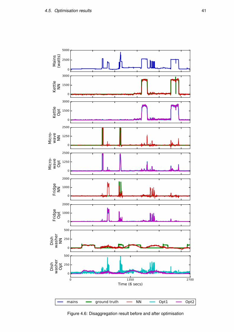
4.5. Optimisation results 41

0 500 1000 1500 2000 2500

0

2500

5000

Main

s(w

att

s)

0 500 1000 1500 2000 2500

0

1500

3000

Kett

leN

N

0 500 1000 1500 2000 2500

0

1500

3000

Kett

leO

pt

0 500 1000 1500 2000 2500

0

1250

2500

Mic

ro-

wave

NN

0 500 1000 1500 2000 2500

0

1250

2500

Mic

ro-

wave

Opt

0 500 1000 1500 2000 2500

0

1000

2000

Frid

ge

NN

0 500 1000 1500 2000 2500

0

1000

2000

Frid

ge

Opt

0 500 1000 1500 2000 2500

0

250

500

Dis

hw

ash

er

NN

0 1350 2700

Time (6 secs)

0

250

500

Dis

hw

ash

er

Opt

mains ground truth NN Opt1 Opt2

Figure 4.6: Disaggregation result before and after optimisation


0 100 200 300 400 500 600 700

0

2500

5000

Main

s(w

att

s)

Kettle

0 350 700

0

1500

3000

Opt2

(watt

s)

0 350 700

Time (6 secs)

0

1500

3000

Opt3

(watt

s)

0 100 200 300 400 500

0

1500

3000Fridge

0 250 500

0

50

100

0 250 500

Time (6 secs)

0

50

100

mains ground truth NN Opt2 Opt3

Figure 4.7: Disaggregation result before and after optimisation

0.0 0.5 1.0 1.5 2.0 2.5 3.0 3.5 4.0

0

0.5

1

F1score 0.

89

0.86

0.88

0.87

Kettle

0.0 0.5 1.0 1.5 2.0 2.5 3.0 3.5 4.0

0

0.5

1

Precisionscore 1.

0

0.76 1.0

1.0

0.0 0.5 1.0 1.5 2.0 2.5 3.0 3.5 4.0

0

0.5

1

Recallscore 0.

80 1.0

0.79

0.77

0.0 0.5 1.0 1.5 2.0 2.5 3.0 3.5 4.0

0

0.5

1

Accuracyscore 0.

99

0.99

0.99

0.99

0.0 0.5 1.0 1.5 2.0 2.5 3.0 3.5 4.0

0

100

200Mean

absoluteerror

(watts) 27.6

22.6

22.0

21.4

0.0 0.5 1.0 1.5 2.0 2.5 3.0 3.5 4.0

0.0

0.2

0.4

0.6

0.8

1.0

0.61

0.57

0.61

0.61

Fridge

0.0 0.5 1.0 1.5 2.0 2.5 3.0 3.5 4.0

0.0

0.2

0.4

0.6

0.8

1.0

0.67

0.61

0.67

0.67

0.0 0.5 1.0 1.5 2.0 2.5 3.0 3.5 4.0

0.0

0.2

0.4

0.6

0.8

1.0

0.56

0.53

0.55

0.56

0.0 0.5 1.0 1.5 2.0 2.5 3.0 3.5 4.0

0.0

0.2

0.4

0.6

0.8

1.0

0.75

0.68

0.75

0.75

0.0 0.5 1.0 1.5 2.0 2.5 3.0 3.5 4.0

0

50

100

150

200

29.6

40.6

27.9

28.0

0.0 0.5 1.0 1.5 2.0 2.5 3.0 3.5 4.0

0.0

0.2

0.4

0.6

0.8

1.0

0.49

0.51

0.49

0.49

Microwave

0.0 0.5 1.0 1.5 2.0 2.5 3.0 3.5 4.0

0.0

0.2

0.4

0.6

0.8

1.0

0.33

0.83

0.34

0.34

0.0 0.5 1.0 1.5 2.0 2.5 3.0 3.5 4.0

0.0

0.2

0.4

0.6

0.8

1.0

0.88

0.37

0.87

0.84

0.0 0.5 1.0 1.5 2.0 2.5 3.0 3.5 4.0

0.0

0.2

0.4

0.6

0.8

1.0

0.98

0.98

0.98

0.98

0.0 0.5 1.0 1.5 2.0 2.5 3.0 3.5 4.0

0

50

100

150

200

37.6

27.3

26.4

26.4

0.0 0.5 1.0 1.5 2.0 2.5 3.0 3.5 4.0

0.0

0.2

0.4

0.6

0.8

1.0

0.39

0.31

0.39

0.39

Dishwasher

0.0 0.5 1.0 1.5 2.0 2.5 3.0 3.5 4.0

0.0

0.2

0.4

0.6

0.8

1.0

0.25

0.93

0.25

0.25

0.0 0.5 1.0 1.5 2.0 2.5 3.0 3.5 4.0

0.0

0.2

0.4

0.6

0.8

1.0

0.94

0.18

0.94

0.94

0.0 0.5 1.0 1.5 2.0 2.5 3.0 3.5 4.0

0.0

0.2

0.4

0.6

0.8

1.0

0.79

0.71

0.80

0.79

0.0 0.5 1.0 1.5 2.0 2.5 3.0 3.5 4.0

0

50

100

150

200

33.1

18.2

17.1

16.9

NN output Optimisation 1 Optimisation 2 Optimisation 3

Figure 4.8: Metrics comparison of different optimisation approaches

Chapter 5

Conclusion and Discussion

5.1 Remarks and observations

This project built and trained different types of neural networks for energy disag-

gregation. The networks achieved great results when the input windows contain no

more than one full activation and got better performance than similar work [11]. High

power consumption appliances like kettle and microwave are relatively easy to detect,

while long operation time and low power demand appliances like fridge and washing

machine are hard to detect. Stacked denoising autoencoders perform generally better

than LSTMs and multilayer perceptrons are sufficient for simple appliances like kettle.

The synthetic data has no significant effect on the test houses seen during training, but

would show advantages when applied to unseen houses and future work.

Three optimisations were carried out on the results of the neural network predic-

tions. The optimisations have greatly lowered the mean absolute error of disaggrega-

tion results. They are able to correct some negative predictions to zeros and correct

some false positives if the sum of all appliances are larger than the mains, which im-

prove the prediction results.

5.2 Drawbacks and limitations

The activations for some appliances like dish washer and washing machine are not

adequate, this project solved this by randomly duplicating these activations. This, how-

ever, hurts the generalisation ability. Also, the training data is generated with ’simple’

constrains, and will be poor at complex situations. When applying the networks on a

continuous period of time, the inputs will include many situations that hasn’t been seen

43

44 Chapter 5. Conclusion and Discussion

during training: more than one activations, the activation is cut off, etc. The network

performance will be greatly influenced by these cases. To minimise possible errors,

the disaggregation windows were moved at a stride of the window width. The size of

neural networks increases exponentially with the input window width, which makes it

computationally expensive to train and evaluate these networks.

5.3 Further work

There is still a lot of work can be done in the future to improve the results. For

example, the networks can be trained on larger and more complex data set, which

include conditions that are described above. Also, the proportion of negative samples

in training set can be increased (such as 70% to 80%), which will be more similar to

the cases in real applications. What’s more, appliance specific data from more houses

and cover more variations will be very helpful in generalising the networks.

As the results show, complex and big neural networks do not guarantee good dis-

aggregation performance, limited by the data and compute resources. Small and naive

networks will be sufficient for appliances with simple load signatures like kettle, while

large and special networks can be used for multiple state appliances like microwave

and washing machine. Miniaturization of large networks will be meaningful in terms

of application, further work can be done on how different sample rates and window

widths affect the disaggregation results. Networks can be trained to predict only the

value in the middle of the window would be a great approach, as there will be much

fewer parameters, easier to train and the training data will be much more compact,

because the targets are only scalars, which will be windowwidth times smaller than the

current approach.

During the training, it was found that some type of networks are sensitive to the

initialisation, which suggests that unsupervised pretraining before supervised training

are likely to help in these cases. Networks of more types of appliances can be trained,

and this allows better use of the ’less than the mains’ prior constraints. Last but not

least, hyper parameters like layer of networks, number of hidden units can be cross

validated, and the architectures of the networks can be appliance-dependent.

Bibliography

[1] Carrie Armel. Energy disaggregation. Precourt Energy Efficiency Center, Stan-

ford, 2011.

[2] Nipun Batra, Jack Kelly, Oliver Parson, Haimonti Dutta, William Knottenbelt,

Alex Rogers, Amarjeet Singh, and Mani Srivastava. Nilmtk: an open source

toolkit for non-intrusive load monitoring. In Proceedings of the 5th international

conference on Future energy systems, pages 265–276. ACM, 2014.

[3] Karen Ehrhardt-Martinez, Kat A Donnelly, Skip Laitner, et al. Advanced me-

tering initiatives and residential feedback programs: a meta-review for house-

hold electricity-saving opportunities. American Council for an Energy-Efficient

Economy Washington, DC, 2010.

[4] Michael Grant, Stephen Boyd, and Yinyu Ye. Cvx: Matlab software for disci-

plined convex programming, 2008.

[5] Alex Graves. Neural networks. In Supervised Sequence Labelling with Recurrent

Neural Networks, pages 15–35. Springer, 2012.

[6] George W Hart. Residential energy monitoring and computerized surveillance

via utility power flows. IEEE Technology and Society Magazine, 8(2):12–16,

1989.

[7] http://deeplearning.net/software/theano/. Theano webpage, 2016.

[8] http://www.energyoracle.org/project.html. Ideal home energy advice project,

2016.

[9] Po-Sen Huang, Xiaodong He, Jianfeng Gao, Li Deng, Alex Acero, and Larry

Heck. Learning deep structured semantic models for web search using click-

through data. In Proceedings of the 22nd ACM international conference on

45

46 Bibliography

Conference on information & knowledge management, pages 2333–2338. ACM,

2013.

[10] Jack Kelly and William Knottenbelt. Uk-dale: A dataset recording uk domestic

appliance-level electricity demand and whole-house demand. ArXiv e-prints, 59,

2014.

[11] Jack Kelly and William Knottenbelt. Neural nilm: Deep neural networks applied

to energy disaggregation. In Proceedings of the 2nd ACM International Confer-

ence on Embedded Systems for Energy-Efficient Built Environments, pages 55–

64. ACM, 2015.

[12] Alex Krizhevsky, Ilya Sutskever, and Geoffrey E Hinton. Imagenet classification

with deep convolutional neural networks. In Advances in neural information

processing systems, pages 1097–1105, 2012.

[13] Yann A LeCun, Leon Bottou, Genevieve B Orr, and Klaus-Robert Muller. Effi-

cient backprop. In Neural networks: Tricks of the trade, pages 9–48. Springer,

2012.

[14] Warren S McCulloch and Walter Pitts. A logical calculus of the ideas immanent

in nervous activity. The bulletin of mathematical biophysics, 5(4):115–133, 1943.

[15] Gregoire Mesnil, Yann Dauphin, Kaisheng Yao, Yoshua Bengio, Li Deng, Dilek

Hakkani-Tur, Xiaodong He, Larry Heck, Gokhan Tur, Dong Yu, et al. Us-

ing recurrent neural networks for slot filling in spoken language understand-

ing. IEEE/ACM Transactions on Audio, Speech, and Language Processing,

23(3):530–539, 2015.

[16] Michael A Nielsen. Neural networks and deep learning. URL:

http://neuralnetworksanddeeplearning. com/.(visited: 01.11. 2014), 2015.

[17] Department of Energy Climate Change. Smart meter roll-out for the domestic

and small and medium non-domestic sectors (gb): Impact assessment. GOV.UK,

2014.

[18] Department of Energy Climate Change. Consumer prices index uk. GOV.UK,

2016.

Bibliography 47

[19] University of Illinois at Urbana-Champaign. Center for Supercomputing Re-

search, Development, and G Cybenko. Continuous valued neural networks with

two hidden layers are sufficient. 1988.

[20] David Silver, Aja Huang, Chris J Maddison, Arthur Guez, Laurent Sifre, George

Van Den Driessche, Julian Schrittwieser, Ioannis Antonoglou, Veda Panneershel-

vam, Marc Lanctot, et al. Mastering the game of go with deep neural networks

and tree search. Nature, 529(7587):484–489, 2016.

[21] Karen Simonyan and Andrew Zisserman. Two-stream convolutional networks

for action recognition in videos. In Advances in Neural Information Processing

Systems, pages 568–576, 2014.

[22] Richard Socher, Alex Perelygin, Jean Y Wu, Jason Chuang, Christopher D Man-

ning, Andrew Y Ng, and Christopher Potts. Recursive deep models for semantic

compositionality over a sentiment treebank. In Proceedings of the conference on

empirical methods in natural language processing (EMNLP), volume 1631, page

1642. Citeseer, 2013.

[23] Yaniv Taigman, Ming Yang, Marc’Aurelio Ranzato, and Lior Wolf. Deepface:

Closing the gap to human-level performance in face verification. In Proceed-

ings of the IEEE Conference on Computer Vision and Pattern Recognition, pages

1701–1708, 2014.

[24] Pascal Vincent, Hugo Larochelle, Isabelle Lajoie, Yoshua Bengio, and Pierre-

Antoine Manzagol. Stacked denoising autoencoders: Learning useful represen-

tations in a deep network with a local denoising criterion. Journal of Machine

Learning Research, 11(Dec):3371–3408, 2010.

[25] Mingjun Zhong, Nigel Goddard, and Charles Sutton. Signal aggregate con-

straints in additive factorial hmms, with application to energy disaggregation.

In Z. Ghahramani, M. Welling, C. Cortes, N. D. Lawrence, and K. Q. Wein-

berger, editors, Advances in Neural Information Processing Systems 27, pages

3590–3598. Curran Associates, Inc., 2014.

[26] Ahmed Zoha, Alexander Gluhak, Muhammad Ali Imran, and Sutharshan Ra-

jasegarar. Non-intrusive load monitoring approaches for disaggregated energy

sensing: A survey. Sensors, 12(12):16838–16866, 2012.

a deep learning approach to identifying household

Documents