a deep learning model for automatic … · a deep learning model for automatic image texture...
TRANSCRIPT

A DEEP LEARNING MODEL FOR AUTOMATIC IMAGE TEXTURE
CLASSIFICATION: APPLICATION TO VISION-BASED AUTOMATIC AIRCRAFT
LANDING
Khai Ping, Lai
Submitted in fulfilment of the requirements for the degree of
Master of Engineering by Research
Science and Engineering Faculty
Queensland University of Technology
2016

A Deep Learning Model for Automatic Image Texture Classification: Application to vision-based Automatic Aircraft Landing i
Keywords
Deep Learning, Deep Recurrent Neural Network, Long Short Term Memory (LSTM), Machine Learning, Physics, Texture Classification, The Mechanism of Camera, xy Chromaticity Diagram, Unmanned Aerial Vehicle (UAV).

A Deep Learning Model for Automatic Image Texture Classification: Application to vision-based Automatic Aircraft Landing ii
Abstract
The Long Short Term Memory architecture is a powerful sequence learner,
which principally has the ability to memorize relevant events over time. These
attributes make Long Short Term Memory approaches more applicable for analysing
huge and complex datasets. However, this computationally powerful algorithm has
not been perceived as useful for image analysis as it is for handwriting recognition.
This project investigates the LSTM architecture for image texture classification. This
thesis also discusses concepts and considerations, which influence data organization
before feeding into the Machine Learning technique. We have achieved performance
figures with a Mean Square Error of 0.095 (Experiment 1). The project also shows
that by recognising pixels’ location via the xy Chromaticity Diagram, small sample
sizes of datasets are sufficient to perform texture classification (Experiment 2). The
findings of this research will eventually apply in image-regions texture classification,
to assist unmanned aerial vehicles (UAVs) to land safely in an emergency situation.
The overall findings demonstrates that above 95% of labels are correctly classified
by the LSTM algorithm, for each result using xy Chromaticity colour space as pre-
processing stage.

A Deep Learning Model for Automatic Image Texture Classification: Application to vision-based Automatic Aircraft Landing iii
Table of Contents
Keywords..............................................................................................................................i
Abstract ...............................................................................................................................ii
Table of Contents ............................................................................................................... iii
List of Figures ...................................................................................................................... v
List of Tables ..................................................................................................................... vii
Statement of Original Authorship ......................................................................................viii
Acknowledgements ............................................................................................................. ix
Chapter 1: Introduction .......................................................................................... 1
1.1 Research Objective..................................................................................................... 3
1.2 Thesis Outline ............................................................................................................ 4
1.3 Summary.................................................................................................................... 4
Chapter 2: Literature Review ................................................................................. 5
2.1 Deep Recurrent Neural Network ................................................................................. 6 2.1.1 An Overview of Machine Learning ................................................................... 6 2.1.2 Why Deep Learning ......................................................................................... 9 2.1.3 Why Artificial Neural Network....................................................................... 10 2.1.3.1 Topology of Neural Network – Feedforward vs Recurrent ................... 12 2.1.4 Why Long Short Term Memory Architecture.................................................. 14 2.1.4.1 The Importance of Long Term Memory .............................................. 15 2.1.4.2 The Ability of Forgetting .................................................................... 24
2.2 Texture Feature Extraction ....................................................................................... 28 2.2.1 The Methods of Feature Extraction ................................................................. 29 2.2.2 Limitations and Concerns ............................................................................... 33
2.3 The xy Chromaticity Colour Space ........................................................................... 40
2.4 Summary.................................................................................................................. 45
Chapter 3: The Long Short Term Memory .......................................................... 47
3.1 The LSTM Architecture ........................................................................................... 49 3.1.1 Peephole Connection ...................................................................................... 51
3.2 The LSTM Forward and Backward Pass Equations................................................... 51
3.3 Summary.................................................................................................................. 56
Chapter 4: Research Design .................................................................................. 57 4.1 Problem Background ................................................................................................ 57
4.2 Datasets Background ................................................................................................ 59 4.2.1 Dataset 1 ........................................................................................................ 59 4.2.2 Dataset 2 ........................................................................................................ 60
4.3 Datasets Organization............................................................................................... 62 4.3.1 How the LSTM architecture processes data .................................................... 62

A Deep Learning Model for Automatic Image Texture Classification: Application to vision-based Automatic Aircraft Landing iv
4.4 The Steps of creating Datasets .................................................................................. 67
4.5 Summary.................................................................................................................. 70
Chapter 5: Experiments & Results ....................................................................... 71 5.1 Experiment 1 ............................................................................................................ 72
5.2 Experiment 2 ............................................................................................................ 74
5.3 Experiment 3 ............................................................................................................ 77
5.4 Summary.................................................................................................................. 85
Chapter 6: Conclusion & Future Work ................................................................ 87 6.1 Future Work ............................................................................................................. 87
6.1.1 Machine Learning Technique – Neural Network Architecture ......................... 87 6.1.1.1The layer of Max-pooling .................................................................... 87 6.1.1.2 Weight Guessing ................................................................................. 88 6.1.2 Object Recognition ......................................................................................... 89 6.1.2.1The Physics Theory may consider being useful at this stage ................. 89 6.1.2.1The Matrix Theory may be used as geometric or shape comparison ...... 90
Bibliography .......................................................................................................... 93
Appendices ............................................................................................................ 99 Appendix A The Steps of constructing Datasets ........................................................ 99
Appendix B The Confusion Matrices of 7 Images ................................................... 104

A Deep Learning Model for Automatic Image Texture Classification: Application to vision-based Automatic Aircraft Landing v
List of Figures
2.1 The basic principles of bagging ...................................................................................... 8
2.2 The basic structure of a neuron in an Artificial Neural Network ................................... 11
2.3a Multilayer Perceptron (MLP) ..................................................................................... 13
2.3b Recurrent Neural Network .......................................................................................... 13
2.4 Recurrent Neural Network Connections ....................................................................... 16
2.5 The Vanishing gradient problem for RNNs ................................................................... 19
2.6 A form of RNN with a self-connection ........................................................................ 20
2.7 The self-recursive loop is suggested to set as the weight of 1.0 ..................................... 23
2.8 The architecture of Long Short Term Memory .............................................................. 24
2.9 The usefulness of removing the irrelevant information .................................................. 26
2.10 A general framework to perform texture classification ................................................ 28
2.11 The effect of scale and rotation on textures ................................................................. 32
2.12 Comparison regions between light-detected and light-undetected ................................ 33
2.13 The demonstration of optical illusion .......................................................................... 34
2.14 The process of transforming data into different space .................................................. 37
2.15 Colour is the human perception ................................................................................. 40
2.16 The datasets depends on lighting condition ................................................................. 41
2.17 The colour spaces conversion between the RGB values to the xy Chromaticity ........... 43
2.18 The comparison the datasets between the RGB Colour Space and the xy Chromaticity Diagram ............................................................................................................................. 44
3.1 Vanishing gradient problem for RNNs .......................................................................... 47
3.2 Preservation of gradient information by LSTM ............................................................. 47
3.3 The basic structure of LSTM architecture ..................................................................... 50
3.4 This Figure shows as reference for forward pass calculation ......................................... 52
4.1 The chart flow of final site selestion for emergency landing .......................................... 57
4.2 The output of the candidate landing site selection ........................................................ 56
4.3 Classification result on a sample image taken from one of the datasets .......................... 62
4.4 The datasets depends on lighting condition ................................................................... 63
4.5 An example of sub-images organization ...................................................................... 66
4.6 The diagram of datasets construction ............................................................................ 69
5.1 The performance of the Neural Network architecture based on MATLAB ................... 75
5.2 An example of turning all pixels’ values to the location representation based on the Diagram ............................................................................................................................ 76
5.3 A result produced by the xy Chromaticity Diagram....................................................... 77
5.4 A sample of the datasets ............................................................................................... 78

A Deep Learning Model for Automatic Image Texture Classification: Application to vision-based Automatic Aircraft Landing vi
5.5 A part of the xy Chromaticity Diagram ......................................................................... 79
5.6 A result produced by the LSTM algorithm which the input is organised based on the xy Chromaticity Diagram ........................................................................................................ 82
5.7 A result produced by the LSTM algorithm which the input is organised based on the xy Chromaticity Diagram ........................................................................................................ 83
5.8 A result produced by the LSTM algorithm which the input is organised based on the xy Chromaticity Diagram ........................................................................................................ 84

A Deep Learning Model for Automatic Image Texture Classification: Application to vision-based Automatic Aircraft Landing vii
List of Tables
4.1 Dataset 1 ...................................................................................................................... 59
4.2 Dataset 2 ...................................................................................................................... 61
5.1 The result of the different combination of the LSTM architecture ................................. 73
5.2 only use for referencing ................................................................................................ 80
5.3 The precision and the recall results for evaluating the performance of the LSTM multi-class classification. ............................................................................................................. 81

A Deep Learning Model for Automatic Image Texture Classification: Application to vision-based Automatic Aircraft Landing viii
Statement of Original Authorship
The work contained in this thesis has not been previously submitted to meet
requirements for an award at this or any other higher education institution. To the
best of my knowledge and belief, the thesis contains no material previously
published or written by another person except where due reference is made.
Signature: QUT Verified Signature
Date: August 2016

A Deep Learning Model for Automatic Image Texture Classification: Application to vision-based Automatic Aircraft Landing ix
Acknowledgements
I thank my principal supervisor Dr. Luis Mejias Alvarez for sharing his
knowledge, guidance and supports. Also, thank you to ARCAA Director Dr. Duncan
Campell who was the associate supervisor during the research.
I would like sincerely thank you to Pedro Pablo Plazas Rincon, Dr. Glenn
Fulford, Leelee Heng, Jasmin Lim and Camran Boyle who dedicated their time and
effort to assist me in any manners, this research had not been possible without their
supports. I want to thank to Dr. Christian Long from the Academic Language and
Learning Service for his support with the edition and correction of my monograph. In
addition, many thanks go to the Engineering and Library Staffs for their excellent
service during this time. A special mention goes to my fellows Research colleagues
and friends (Alex Bewley, Zhang Fang Yi, Tim Molloy and etc.) in both ARCAA
and Engineering Faculty for inspiring me and keep me on track, as well as millions
of thanks to QUT.
Finally, I have to thank my lovely family: mother Ai Mooi, father Boon Fat,
sister Khai Li, and two brothers Jing Liang & Jing Jie, thank you so much for their
constant encouragement, love and sincerity, which allow me fully focus on pursuing
my dreams.
Chapter 1: Introduction 1
Chapter 1: Introduction
Deep Learning (DL) is a hierarchical Machine Learning method based on a set
of algorithms to extract multiple levels of features or, high-level representations in
data that aim to move away from heavy handcrafted features through end-to-end
learning on raw data. The idea of DL is also followed by the assumptions that the
observed data interacts with a set of factors, which can be learnt from one layer to
another by arranging the data into multiple levels corresponding to the levels of
representations. The whole learning process forms the credit assignment path (CAP)
that describes the series of possible connections between input and output
(Schmidhuber, 2014, p. 88), known as Deep Learning architecture.
These ideas developed in Deep Learning have also assisted Machine Learning
(ML) architectures move forward to function autonomously with a minimal human
intervention, and makes ML techniques well-suited for autonomous systems such as
UAVs. Today, many civilian tasks that include surveillance or rescue are assisted
and achieved by UAVs. However, the current technology used in UAVs is still
strictly instructive and highly context dependent, real-time decision making is nearly
unachievable. For these reasons, many restrictions have been applied to civilian
UAVs, due to the lack of Equivalent Levels of Safety to manned aircraft.
In order to develop an adaptable on-board system, Deep Machine Learning
techniques were explored and acknowledged as a potential solution for our problem.
Many great works have been delivered by the Machine Learning community, but
most of the research focus on internal architectures or model enhancement in order to
suit specific tasks and hence, restricted to certain data types range. As UAVs
(machines or robots) rely on different sensors to detect its surroundings, it is useful if
there is a ML algorithm that could possibly integrate one data type with another data
type. Furthermore, if ML technique claimed to mimic functionality as human brain,
then the usefulness of the technique must be broad enough to cope with different
scenarios. Having said that, selecting a multipurpose algorithm requires a loaded-
information understanding before integrating stage can be reached. For this reason,
this project aims to identify a ML architecture, which potentially becomes a central

Chapter 1: Introduction 2
machine to analyse many data types. In addition, this ML architecture is extendable
to learn attributes to reduce context or data dependence on handcrafted features.
Data reflects information; and information derives decision making. The on-
board system of an UAV constantly measures for decisions to perform a series of
tasks. This task includes classifying imaging data to distinguish possible regions for
an emergency landing, and serves exactly the main application for this project. Many
Machine Learning techniques have been widely used in terrain classification through
digital image analysis (Mejias, 2014, Background, para. 3). However, computing a
characteristic of a digital image that is numerically describable is complex.
Technically, colour images are just a group of pixels represented by numbers.
Numbers change as detected colour change; while detected colours change as light
direction, object’s properties, or viewpoints change. Intuitively, datasets have left a
great burden for modelling to learn relevant features, which can lead to weeks or
months’ of computing power. The issues of coping with complex relationship within
the data partly explain why mathematical models can grow into really complex
forms. Therefore, using digital images for decision making, in fact, introduces
another issue and often complicates ML techniques to search for patterns.
To deal with dataset issues, it is necessary to have a solid understanding of the
input from the dataset perspective. The project approaches the problem from ML
perspective, identifying a multi-usage algorithm that will play a big part of this
thesis. Subsequently, the concepts that form digital images will generally be
explored, and this brief “walkthrough” will help to organise dataset patterns based on
numeric, data and algorithmic explanations that will be further discussed in literature
review. Once dataset is translated into patterns, small dataset for processing is
achievable as pattern enables modelling to converge quickly. The findings from both
ML technique and dataset will eventually be applied in a larger project, to assist
UAVs land safely in an emergency situation based on image-region classification.

Chapter 1: Introduction 3
1.1 RESEARCH OBJECTIVE
There are two main research objectives for this project. The first objective is to
identify a robust Deep Learning architecture, which possesses the potential capability
to develop into a central machine that can analyse different data types. This session
will analyse a series of relevant ML topics that contribute to the DL architecture
selection.
The second objective aims to understand how information can be extracted
from digital images, so that it can be numerically translated into patterns before
feeding into a ML algorithm. As detected information presented in digital images are
all encoded into numeric representations that fit into electronic environment
(hardware), as well as human usage (perception); this project will break imaging
dataset into numeric, data and algorithmic aspects to assist in explaining the process
of translating data into patterns. Also, the light-and-matter interaction is another
important stage happens before information is detected, which requires a sounded
understanding; yet, it is not the focus for this project. For these reasons, this session
broadly discusses cross-disciplinary concepts that contribute to data organisation.
These two research questions give rise to the following research focus:
1. How the identified algorithm – the Long Short Term Memory
architecture, can be used for automatic image texture classification? As
the Long Short Term Memory technique is merely proposed in image
recognition, it is difficult to make direct comparisons with existing
results or claim for a better approach. This project aims to provide
reasoning that the LSTM architecture also has the ability to perform
image classification, as long as the imaging dataset can be structured
into patterns.
2. How the proposed pre-processing technique - xy Chromaticity Diagram
assists in data representation and hence, small sample size datasets is
sufficient to be learnt by Machine Learning techniques.

Chapter 1: Introduction 4
1.2 THESIS OUTLINE
The thesis is generally structured around three main areas: Deep Machine
Learning approach, the limitations and concerns behind the imaging data, and the
main application of this research. Chapter 2 briefly reviews the scope of Machine
Learning techniques in general, and the process of identifying the choice of a Deep
Learning model in particular. Chapter 2 also discusses existing methods to extract
texture features and highlighting limitations and concerns behind image data.
Although we do not investigate the limitations and concerns in detail, it provides the
reasoning how the great variance within datasets can be stabilised and prepared for
further usage. Chapter 3 describes the LSTM architecture with a special mention of
the possible future usage of peephole connection. The LSTM equations for
performing the activation and backpropagation will also be provided for
understanding. Chapter 4 presents the background of the datasets, data designation
based on the xy Chromaticity Diagram as well as the steps for constructing datasets.
Chapter 5 describes the experiments and results that validate our investigations. This
section will also demonstrate the applicability of the research to assist UAVs to
perform image-regions texture classifications. Chapter 6 provides conclusions and
directions of future work.
1.3 SUMMARY
This chapter aimed at delivering a general framework of the entire research.
The research objectives were presented, which proposes new methods for both
Machine Learning approach (the LSTM) and technique for feature extraction (xy
Chromaticity Diagram). Next section will turn the focus to Literature Review.

Chapter 2: Literature Review 5
Chapter 2: Literature Review
The literature review chapter will be broadly divided into two parts: Machine
Learning approaches and the input data - images. For the Machine Learning
approach, this chapter will provide a relevant insight in order to select a Deep
Learning model that possesses the attributes to develop into multi-usage architecture.
The part of input data focuses on the datasets which will be further categorised into
two main sections: texture feature extraction and the science behind imaging data.
This chapter begins with Machine Learning approach: Deep Recurrent Neural
Networks (section 2.1) and reviews literature on the following topics: An overview
of Machine Learning, why Deep Learning approach is important; what makes
Artificial Neural Network a better approach among other Machine Learning
techniques, and why the Long Short Term Memory (LSTM) architecture is selected
as the Machine Learning technique for this project, especially the LSTM is not a
commonly used technique to analyse imaging datasets.
Section 2.2 generally reviews the common techniques that use to extract
texture feature, which aims to provide a brief background on texture feature
extraction before the datasets can be classified by Machine Learning techniques.
This section briefly discusses the challenges in finding patterns in the input data.
This section also discusses the sciences of forming digital images through a general
understanding, which affects the way the imaging datasets can be structured. This
section also closely relates to the future work under subsection: “Object
Recognition” that will be presented at the end of the thesis.
Section 2.3 introduces the use of xy Chromaticity Diagram as the feature
extraction technique for this project, explains the key features and its usefulness
provided by the xy Chromaticity Diagram in particular.
Section 2.4 summarises the chapter and concludes with a clear direction of the
project’s focus.

Chapter 2: Literature Review 6
2.1 DEEP RECURRENT NEURAL NETWORK
“A computer program is said to learn from experience E with respect to some
class of tasks T and performance measure P, if its performance at tasks in T, as
measured by P, improves with experience E”.
This is a notable quotation by Tom M. Mitchell (1997) towards Machine
Learning. Perhaps, this is the turning point for Artificial Intelligence that led to the
emergence of Machine Learning, since then it slowly shifted the focus from
cognitive to operational terms. Nowadays, Machine Learning has become a field that
is all about making machines to learn. Therefore, Machine Learning can be
overwhelming and often lead to confusion. This section first presents an overview of
Machine Learning that relates to the objective of identifying a multi-usage Deep
Learning architecture. The proceeding subsections will focus on why Deep Learning
is considered, how neural network architecture is favoured, and what makes the Long
Short Term Memory architecture becomes the choice among all the techniques.
2.1.1 An Overview of Machine Learning
Machine Learning is concerned with the development of approaches that
computers learn based on given inputs (features, characteristics, but hardly presented
in raw data). These approaches can be statistical or genetic algorithms that search for
patterns and relationships within datasets, known as training process. After the
training process, the algorithms can output models, parameters, weights or thresholds
which describe the relationships among the input data. Machine Learning techniques
are said to be able to learn if the technique successfully find a describable
relationship between inputs and outputs. Any output will eventually allow the
machine to act accordingly and hence, achieve the goals of prediction, optimisation,
recognition, classification or other decision making for the later use.
As objectives can vary in different applications, many approaches have been
introduced to Machine Learning, frequentist and probabilistic theories in particular.
For instance, Fisher’s linear discriminant, Principal Component Analysis (PCA),
factor analysis, Canonical Discriminant Analysis (CDA) all use statistical method to
identify separable features which can linearly differentiate between the two data
classes. Tasks can also be based on probabilistic theories, which use probability
distribution to classify the input data including conditional assumptions in their

Chapter 2: Literature Review 7
measurement, and giving its own right or closer descriptions for the targeted
problems (Hastie, Tibshirani, Friedman, 2009). For example, the likelihood of
raining today depends on the day before, or seasons or experience. Typical
probabilistic classifiers that seek relationships in the input data are Naïve Bayes,
logistic regression or Bayesian decision trees. Generally, all statistical or
mathematical models have the ability to distinguish data, according to its category
during the learning process if the targeted labels or values were provided, which is
known as supervised learning.
In some situations, datasets can be so large and complex that users have little
or no knowledge to approach their problems. In such situation, techniques applied in
Machine Learning can be employed to search for patterns or characteristics among
data. This learning process is considered unsupervised learning. This searching (or
learning) process needs to seek and summarise the key features of the datasets
without any upfront result present in the calculation. For example, k-means
clustering, which uses a centroid-based approach to partition data objects based on
the cluster central vector found in the data. Other clustering algorithms may approach
the datasets based on connectivity, density, or distribution of the data. For example,
Expectation Maximization (EM) defines objects belonging based on Gaussian
distribution models. EM approach can be complex, as they capture correlated and
dependent relations of data which may lead to inseparable due to highly related
attributes.
Other well-known approaches for general problems or specific tasks include:
Classification and Regression Tree (CART), Random Forest, Gradient Boosting
Machines (GBM). These are based on logic approaches that provide a
comprehensive approach to linear Machine Learning problems. The benefit is that
researchers can easily understand the relationship between the nodes which
represents a feature in an instance to be classified. Decision tree also expands into the
rule-based algorithms by having a set of criteria for each path from the root to a node
in a tree. Machine Learning approaches may be also derived from a set of techniques
combined to deal with highly-correlated data. For instance, k-Nearest Neighbour
(kNN) is an instance-based method that combines Principal Component Analysis
(PCA), linear discriminant analysis (LDA), or canonical correlation analysis (CCA)
techniques for the purpose of dimension reduction (pre-processing) to extract

Chapter 2: Literature Review 8
features before performing k-NN algorithm searches (Blake & Jebara, 2009).
Boosting, Booststrapped Aggregation (Bagging), and AdaBoost apply similar ideas
called ensemble, to make overall prediction by combining multiple independently
trained models as illustrated on Figure 2.1. Some methods are specific to purposes
such as dimensionality reduction, for instance, Partial Least Square Regression (PLS)
and Sammon Mapping attempts to reduce dimensionality of data relation to decrease
the complexity in the result.
Figure 2.1: The basic principles of bagging. A combination of multiple trained
models to perform analysis on the relationship between ozone and temperature,
which is adapted from Rousseeuw and Leroy (1986), available at classic datasets,
analyses is performed in R (as cited in Klawonn, Berthold, & Ada, 2009).
Machine Learning techniques have been applied to discover data relationships
at much more challenging levels such as handwriting segmentation or other highly
complex behaviours. Even though Support Vector Machine (SVM) or Gabor filters
were popular choices, which outperformed most learning algorithms across different
applications, the relationship between data or information carried in the data itself
can be so intense that, traditionally used statistical or mathematical models are not
sufficient. Deep Learning is one of the proposed techniques that aim to discover
better representations of the inputs. The idea behind Deep Learning argues that
machine can learn through a hierarchy of features, if data representation can be
organised into a stack of layers according to its levels of abstractions. This argument
has indirectly created the trend of designing Deep Learning architectures, and has

Chapter 2: Literature Review 9
specially rebranded the use for Artificial Neural Networks (Collobert, 2011; Lee,
2014). Deep neural networks including, Convolutional Deep Neural Networks
(Larochelle, Bengio, Louradour, & Lamblin, 2009; Bengio, Courville, & Vincent,
2013; Krizhevsky, Sutskever, & Hinton, 2012; Wang, Yang, Zhu, & Lin, 2013;
Ciresan, Meier, Masci, Gambardella, M., & Schmidhuber, Flexible, 2011; Cimpoi,
Maji, & Vedaldi, 2014; Simonyan, & Zisserman, 2014), Long Short Term Memory
(Hochreiter, & Schmidhuber, 1997; Gers, & Schmidhuber, 2000; Byeon, Wonmin,
Breuel, Thomas, Raue, Federico, & Liwicki, Marcus, 2015; Carlini, 2011; Donahue,
Hendricks, Guadarrama, Rohrbach, Venugopalan, Saenko, & Darrell, 2014) or other
Deep Learning architectures (Greff, Srivastava, & Schmidhuber, 2015; Stollenga,
Byeon, Liwicki, & Schmidhuber, 2015; Graves, Fernandez, & Schmidhuber, 2007;
Graves, Mohamed, & Hinton, 2013; Ciresan, Meier, Gambardella, & Schmidhuber,
2010; Ciresan, Meier, & Schmidhuber, 2012;), have been shown to produce state-of-
the-art results on various tasks. The success of Deep Learning neural networks has
also motivated this project.
Overall, the goal of using Machine Learning techniques is to look for the
relationships within data, e.g. patterns. Many techniques have been suggested to cope
with data complexity, and have competently delivered the results. However, the real-
world data is always flooded with information that depends on many factors. Often,
these data classes need intensive labour, engineering features to pre-process the data
before it can be learnt efficiently by the machine, which leads to the evolution of
Deep Learning, particularly Deep Neural Network. Deep Neural Network (DNN) has
now become one of the leaders among Machine Learning techniques to perform
different complex tasks, for example, object recognition. The contribution from DNN
architectures is undeniable, and there must be reasons. The subsequent sections will
present a better insight of Deep Neural Network. The next section will begin with the
concept behind Deep Neural Network - Deep Learning.
2.1.2 Why Deep Learning
One of the most promising ideas provided by Deep Learning is to focus on the
end-to-end learning process without labour intensive feature labelling. This concept
suggests that complex information can be disentangled through representing features
at different layers (Bengio, Courville, & Vincent, 2013). As layers of representations

Chapter 2: Literature Review 10
are necessary to design the Deep Learning architectures, this process leads to a
consequence of raw-feature-based end-to-end learning (Deng, Yu, 2014).
For these reasons, the ideas developed in Deep Learning have assisted Machine
Learning moving onto an influential trend, which can be proved by many successful
applications. For example, Hinton (2007) showed a multi-layered feedforward neural
network have effectively pre-trained one layer at a time, treating each layer as
an unsupervised restricted Boltzmann machine, supervised backpropagation is then
used for fine-tuning. Other good examples such as a car trained by Deep Learning,
which may allow cars interpret 360° camera views (Talbot, 2015), or researchers
from Google and Stanford enhanced Deep Learning for drug discovery by using data
from a variety of sources (Ramsundar, Kearnes, Webster, Konerding, & Pande,
2015).
Certainly, a Deep Learning architecture is not necessarily the only solution for
complex tasks. For instance, shallow FNNs perceiving large “time windows” of input
events may classify long input sequences, through a well-defined output events to
solve problems involving long time lags between relevant events. Furthermore, the
difficulty of a problem may have little to do with its depth (layered structures). Some
NN with only a few layers may solve deep problems by random weight guessing.
Alternatively, unsupervised learning approaches may be feasible to train an NN
shallow problem before developing into deeper features (Schmidhuber, 2014).
However, if one long-term goal of Deep Learning is to perform a very complex
behaviour such as perception (vision and audition), reasoning, and other intelligent
behaviour (Bengio, & LeCun, 2007); it is essential to produce methods that are
flexible to perform deep or shallow searching. Often, deep architectures are more
capable to shift to shallow architecture, but this may not be the case for a shallow
architecture. Overall, moving away from an intensive handcrafted engineering is the
main goal of applying Deep Learning, and consequently our project. In order to build
a flexible and adaptable Machine Learning technique, Artificial Neural Network
architecture is introduced. The following section will explain how Artificial Neural
Network can behave flexibly and adaptably.

Chapter 2: Literature Review 11
2.1.3 Why Artificial Neural Network
Why Artificial Neural Network (ANN)? Putting biological reasons aside, the
mathematics used in Neural Network (NN) are essentially variants of linear
regression methods dating back to the early 1800s (e.g., Gauss, 1809, 1821;
Legendre, 1805) according to Schmidhuber (2014).
Indeed, the origin of ANNs is inspired by the nature of neurons. From the
collections of signals to sending out the spikes of electrical activity through a long
and thin tube (known as axon), are all artificially abstracted and described as
mathematical functions. The artificial neuron is perceived as the most fundamental
computational unit, as illustrated in Figure 2.2.
Figure 2.2: The basic structure of a neuron in an Artificial Neural Network.
Each neuron will randomly generate and attach a weight ijw , with each accepting
input ja , and summed by the “Input Function” and then passed to “Activation
Function”. The “Activation Function” can be seen as a threshold to decide the
output ia , before sending out to the entire network or successive neurons. Adapted
from “Artificial Intelligence” by Bringsjord, S., 2006. Note: all neurons produce only
1 output, similar to the neurons in the multilayer network, unless it specifies. The
numbers of arrows demonstrate 1 output for 3 different neurons in the next layer.
Each neuron consist of a weight connection ijw , , which will be associated with
the input data ja . In biology, the weight represents the strength of the synapses
between neurons. All the input data attached with a weight will then be summed up
and processed by the activation function. The activation function of a unit intends to

Chapter 2: Literature Review 12
model the average firing rate of spikes found in biological neuron. Once the model
learns the firing rate, the rate will be obtained at “Output” layer and sent to the
successive neuron(s) or the entire Neural Network, which will happen at the “Output
Links”. The numbers of arrows at “Output Links” depend on how many units or
neurons it connects to.
Conceptually, weight indicates the importance of an input. The model of firing
rates allows the input to connect to the environment (network) or the next neuron,
depending on the significance of the input. These are the two critical attributes that
enable mathematics and statistics to perform in a flexible manner such as responding
to dynamic behaviour. Dynamic capability is essential for performing decisions
change to adapt new environment when current input is characteristically different to
the previous one, particularly the real-world data representation depends on many
layers of factors. Imagine, this idea applies to a set of connected neurons; it becomes
a group of mathematical and statistical models which are powerful for computation.
All reasons together have demonstrated the usefulness of Neural Network technique.
2.1.3.1 Topology of Neural Network – Feedforward vs Recurrent
In practice, these small computational units or neurons are connected into
many different forms. ANN architectures without looping connection are known as
Feedforward Neural Networks (FNNs). Well known FNN examples include
perceptron (Rosenblatt, 1958), radial basis function networks (Broomhead and Lowe,
1988), Kohonen maps (Kohonen, 1989), Hopfield nets (Hopfield, 1982), the
multilayer perceptron (MLP) (MLP; Rumelhart et al., 1986; Werbos, 1988; Bishop,
1995), and even Convolutional Neural Network which is highly recognised
architecture within the computer vision community. FNN arranges the units into
layers and only allows input to flow in one direction. The following Figure 2.3a
shows the layout of MLP.
FNN is considered a time window technique which has a fixed window of
recent inputs that can serve as a temporal sequence processing system. Time window
technique is a mathematical function for processing data within certain well-defined
interval. However, this approach has a few drawbacks such as determining the
optimal time window size; while defining time window size is the key to use this
technique. A large input window is also another consideration for tasks with long-
term dependencies, yet again, most of the datasets are long-dependent. One solution

Chapter 2: Literature Review 13
for long-dependent datasets might combine several time windows, provided the exact
long-term dependencies of the task are known, which also create a series of issues.
For example, one crucial component of performing classification is contextual
information. Mathematically, “context” can be seen as constraints (or criteria) that
help the modelling to “manoeuvre” within problems. Instead, this crucial element
presents an issue for standard FNN algorithm, because the architecture layout is only
designed to process one input at the time. When the algorithms only process data in
one direction, the first input layer must be well-defined in order to cover useful
information; yet, the definitions are always unknown. One of the solutions is to
collect information through shifting time-window, this approach suffers from not just
information is distorted as time-window shifts; but also searching the useful range of
contextual information is generally unknown. As a consequence, it goes back to the
question: what is the right time-window size in order to cover as useful range as
possible.
Other issues include fixed windows which are inadequate when a task has
changing long-term dependencies, in turn this defeat the purpose of using NN as a
strict mathematics will have the similar ability to perform a well-defined searching.
In fact, FNN is proved that it has the ability to map a compact input to arbitrary
precision, only if FNN contained a sufficient number of nonlinear units within a
hidden layer (Hornik, Stinchcombe, & White, 1989). Perhaps, the key issue is that
the static layout of connections does not allow FNN to create internal states, has
restricted the previous input to influence the network output over time. In other
words, the layout constrains dynamic behaviour. On the other hand, Recurrent
Neural Network does not suffer from these problems.
Chapter 2: Literature Review 14
(a)
(b)
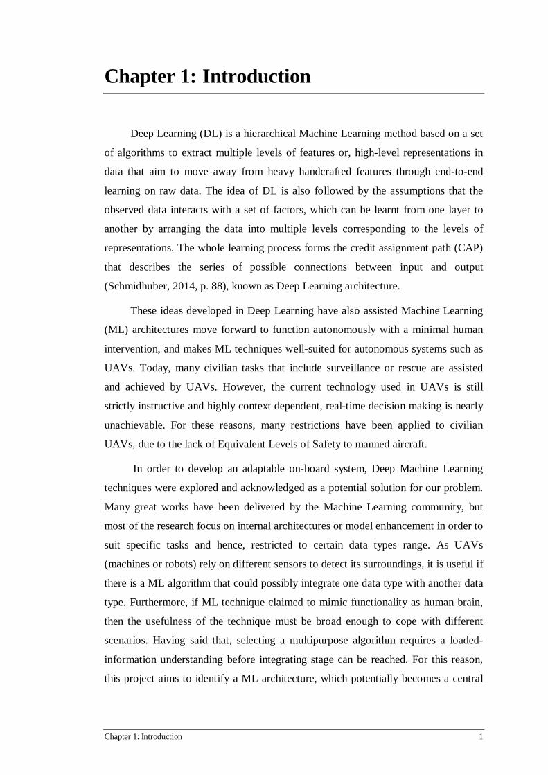
Figure 2.3a: Multilayer Perceptron (MLP). Figure 2.3b: Recurrent Neural Network. Figure
2.3a: The input patterns are presented to the input layer will be propagated through the hidden
layers and to the output layer. Figure 2.3b: A self-recurrent is recursive infinity, and is always
depends on the past. This attribute allows to model data that depend on previous data. If this
concept expanded, the network will be allowed to model a sequence of data. Figure2.3a:
Adapted from “Supervised Sequence Labelling with Recurrent Neural Networks” by Graves,
A., 2007. Figure2.3b: Adapted from “Bidirectional Recurrent Neural Networks” by Xu, J.
In principle, a Recurrent Neural Network (RNN) (Figure 2.3b) can perform
dynamic behaviour through a cyclical connection within the unit or between units.
Unlike FNN, RNN creates an internal state of the network, which allows its internal
memory to process arbitrary sequences of inputs. Although some data types are not
inherently sequential, theoretically, these datasets derive from some sort of pattern
which occurs in a sequential manner (otherwise there are no observable patterns). To
be clear, sequence is not restricted to time-dependency; it also can be state-
dependent, step-dependent, point-dependent, or other pattern dependent as long as it
happens in one entry at a time. In fact, kernel machines learn relationships about the
i th example ( ix , iy ), instead of a fixed set of parameters corresponding to the
features of their input. From a different point of view, a kernel machine learns with
example-dependency. Unfortunately, a kernel machine has no internal states, which
prevents the technique from behaving dynamically. The rationale is also extended to
the choice of algorithms with sequential processing as they are designed to adapt the
change in a series of input data. On top of that, a sequential processor will be
computationally significant as it nicely fits into a computing environment that

Chapter 2: Literature Review 15
follows instructive orders. In short, sequential processing increases computer
performance. Since Recurrent Neural Network fundamentally works as sequential
processing, therefore, we favour RNN architecture to perform image analysis, texture
classification for this project in particular.
2.1.4 Why Long Short Term Memory Architecture
RNN constitutes a very powerful class of computational models as it is capable
of instantiating almost arbitrary dynamics (Siegelmann & Sontag, 1991). Recurrent
networks principally use their feedback connections as the short-term memory to
store representation of the recent input events for over time. As a result, RNNs are
especially promising for tasks that require learning how to use memory, which points
out exactly what we are looking for.
However, the ability to learn to remember did not practically work well for the
standard RNN, especially when long times lag between relevant events which make
learning difficult. In other words, any input happened at stage v , do not influence the
output at stage q , this is due to the short-term memory has either faded away or
blown up. This problem is known as the vanishing or exploding problem is because
of back propagated error signals (Werbo, 1982; Linnainmaa, 1970) either shrink
rapidly or grow exponentially (Hochreiter, 1991) in short-term memory. In fact, the
vanishing or exploding problem occurs in shallow layers, which defeats the interest
of building a Deep Learning architecture. To deal with these problems, the Long
Short Term Memory architecture was designed in 1997 by Hochreiter and
Schmidhuber.
2.1.4.1 The Importance of Long Term Memory
The Long Short Term Memory algorithm has the ability to bridge short-term
memory back to at least, 1000 time steps. In other words, short-term memory is now
able to store input events for a reasonably long time. The foundation in the LSTM’s
concept also serves as the base for the group’s very first deep learner (recurrent or
not) to win several international awards (Schmidhuber, 2015). The ability to
memorise events for long period, is one of the key reasons for us to introduce the
Long Short Term Memory (LSTM) architecture. In order to appreciate the
importance of long-term memory can contribute to the Deep Learning ability; the

Chapter 2: Literature Review 16
following subsections will provide a relevant coverage that leads to the development
of the attribute of long-term memory.
2.1.4.1.1 Training and Learning
Most Neural Networks architectures need supervised training in order to learn
internal relationships that allow any arbitrary mapping of input to output, where each
internal relationship is represented by a weight w . The following Figure 2.4
illustrates a type of the Recurrent Neural Networks connections from input to output,
where each neuron has similar functionality as shown on Figure 2.2 in section 2.1.3.
Figure 2.4 Recurrent Neural Network Connections. x =input layer, y =output layer,
h =hidden layer, w =weight, w∆ =the change of weight, all subscript next to
w indicates the connection between units, xhw = the connection (weight) from unit
x to unit h . The arrows with solid line are a forward propagation process which
shows the flow of the input data; while the arrows with dashed line are backward
pass. Adapted from “Recurrent Neural Networks” by Wu, Zhirong., 2015.
Training process involves forward and backward process regardless the type of
architecture topology. Conceptually, a network forward propagates activation to
produce an output and eventually it backward propagates error (Figure 2.4), and
determines weight changes before updating the new weight.
The objective of training a network is simply tracing the describable
relationship w , between inputs and outputs, through repeatedly taking a small step in
h
y
x
hhw
hyw∆
xyw xhw Forward
Backward
hyw
xyw∆ xhw∆
hhw∆

Chapter 2: Literature Review 17
the direction of the negative error gradient. As a small step is taken, the original
weight changed, the change in weight w can be expressed as:
ijij w
Ew∂∂
−=∆ α (1)
ijw∆ indicates the change of weight that connects from unit i to unit j . Each change
of the weight, will be updated to the previous weight where intentionally moves
towards to the targeted output.
During the training process, the only information the network knows is to “hit”
the targeted output t , but it does not know the actual relationship between the input
and the targeted output. As a result, the initial weight will always be generated
randomly and leave the mathematics and statistics to search for the “real”
relationship. Due to this randomness that cause the difference between the actual
output y and targeted output t , an error function is used to calculate the discrepancy
between the two outputs. A common used error function is the mean squared error:
2)(21 ytE −=
(2)
As negative and positive errors may cancel each other out, the power of two aims to
square these differences before summing, and finally will be scaled by a factor of ½
for convenience.
Eq. (1) states that by taking the derivative of the mean squared error function
with respect to each weight, the new change in weight will be found for each
connection. The process of the network is said to learn after the change of weight has
updated to the previous weight. By doing so, the network needs iteration in the
programming to indicate the step taking, known as learning rateα . The greater
theα , the bigger step it takes, but the measurement may step beyond the targeted
output, which may cause inaccuracy in the calculation. Hence, learning rate is always
set at a very small number. To minimise E , gradient descent learning performs by
multiplying -1 in order to update in the direction of a minimum of the error function.
This information is summarised equally as the right-hand side of Eq. (1).

Chapter 2: Literature Review 18
If the two Eq. (1) and (2) extended to a problem with sequence, the two
functions simply consider each time step carries in the sequence and become the
following expressions:
2])()([21)( ∑ −=
k
kk tytttE (3)
The Eq. (3) shows )(tE represents the error at time t for one sequence component
called pattern. kt is supervised target, where k indexes the output units of the
network with activations ky . For a typical data set consisting of sequences of
patterns, E is the sum of )(tE overall patterns of all sequences in the set.
ijij w
tEtw∂∂
−=∆)()( α
(4)
The Eq. (4) shows the weight change occurs at every time step.
Learning in RNN as optimizing a differentiable objective function E , summed
over all time steps of all sequences. This explanation also strengthens the potential
usefulness of self-recurrent RNN to adapt to multidimensional data types. In
addition, every self-recurrent creates dependency on the past, which can be seen as
opening another “storage” for previous time step. This attribute of RNN is
particularly well-suited for sequential applications, which most of the tasks are often
built from many dependencies. However, the advantage of self-recurrent also leads to
the problems of vanishing and exploding, where the past information either becomes
zeros or so huge that the computer does not recognise. In short, the training process
does not assist the network learn at all.
2.1.4.1.2 The problems of vanishing and exploding
When the standard RNN attempts to apply on the problems with sequences, the
input occurred at many time steps before, will not influence the current output of the
network (Figure 2.5). This problem is known as vanishing or exploding in the
previous memory along the training process (Hochreiter, 1991). In fact, the
calculation decays or explodes exponentially in the first few numbers of layers,
which have constraint the usefulness of Deep Neural Network architecture.
To visualise the vanishing or exploding problem, RNN can be unfolded
through time, which the RNN becomes a standard feedforward neural network with

Chapter 2: Literature Review 19
each layer corresponding to a time step in the RNN as shown in the following Figure
2.5. :
Figure 2.5: The Vanishing gradient problem for RNNs. The shading of the nodes
indicates the sensitivity of the network to the input at that time (the brighter the
shade, the greater the sensitivity). The sensitivity decays exponentially as time
passes, new inputs overwrite the activation of hidden unit and the network ‘forgets’
the first input. These problems eventually cause the network fails to be trained.
Adapted from “Supervised Sequence Labelling with Recurrent Neural Networks” by
Graves, A., 2007.
As the training process does not help the machine learns to remember, the
standard RNN is only fascinated in theory. The vanishing or exploding problem was
also the main reason to cease researchers from using the RNN, perhaps, Artificial
Neural Network architecture. The stagnation of using the ANN architecture had
pointed that the feature of long-term memory is essential to be useful for the real-
world applications, and had led to a series of investigations, particularly backward
propagation.
2.1.4.1.3 Backward Propagation
Training process involves forward and backward propagation, and the network
is said to be able to learn when the weight is found to be describable that links
between the input and the desirable output. As mentioned in section 2.1.4.1.1, the
Outputs
Time Step t t-3 t-2 t-1 t t+1
Hidden Layer
Inputs

Chapter 2: Literature Review 20
weight update process is subject to the calculated change in weights, while the
change in weights depends on the derivative of the mean squared error function with
respect to each weight (Eq. (1)), which is when the problem of vanishing or
exploding occurred. Put it in examples, if the calculated change in weight is zero, the
network is “forever” updating nothing; while the calculated weight is a big number,
the result will move the network way far from the targeted output. To be precise, the
mathematics and statistics behind the network cannot find its own equilibrium.
Therefore, the problem of vanishing or exploding is the key component to be
investigated.
Performing the derivative of the mean squared error function with respect to
each weight is calculated by using chain rule, which is part of the backward pass
process. A backward pass process starts at the output layer of the network, which
aims to perform gradient descent search to minimize the sum squared error of the
entire network. The two popular gradient-based learning methods are
Backpropagation Through Time (BPTT) and Real Time Recurrent Learning (RTRL).
BPTT is used when gradients update for a whole sequence; while RTRL updates for
each frame in a sequence (Wu, 2015). This subsection aims to highlight the problems
of vanishing or exploding, since BPTT is the most widely used for RNN training,
only BPTT will be focused on.
The classical BPTT uses chain rule to trace the change of each weight where
happened anywhere in the entire architecture. For simplicity, a single hidden unit
will be considered and illustrated as Figure 2.6. :
E yθ θ xθ Figure 2.6: A form of RNN with a self-connection. This is a simple form of self-
Hidden Layer
Inputs tx
ty Outputs
th
Chapter 2: Literature Review 21
recursive RNN, where the input tx forward propagates to a single hidden
layer th with some parametersθ , and to the output layer ty . All occurred at time t .
Adapted from “Deep Learning Lecture 12: Recurrent Neural Nets and LSTMs” by
Freitas, N. d., 2015.
This is a simple form of RNN with a self-connection in the hidden layer and map to
one output. tx is input, th is hidden layer, ty is output all occurred at
time t .θ represents some parameters (etc. weight or bias), and )(⋅φ is an activation
function. The forward propagation during training for RNN can be written as:
)( 1−+= ttxt hxh θφθ (5)
)( tyt hy φθ= (6)
Eq. (5) shows the sums of current input attached with some parameters (e.g.
weight w ) and the previous state of hidden layer. Eq. (6) is the output of the network,
which the error function will use the calculated output to compute the difference with
the targeted output.
Figure 2.6, Eq. (5) and Eq. (6) will be used to assist the following calculation.
The following calculation demonstrates the chain rule is implemented by taking the
partial derivative in order to compute the summation of all the partial derivative of
the error with respect to a parameterθ , where n is the numbers of time steps. :
∑= ∂∂
=∂∂ n
t
tEE1
)(θθ
(7)
For eachθ∂
∂ )(tE occurred at that time step, say time step t , is also a summation term
which sums of all parameters occurred before time t , and can be interpreted as:
∑= ∂
∂∂∂
∂∂
∂∂
=∂∂ t
k
k
k
t
t
t
t
hhh
hy
ytEtE
1
)()(θθ
(8)

Chapter 2: Literature Review 22
The Eq. (8) measure howθ that happens at hidden unit k affects the hidden layer at t .
The key component that goes vanishing or exploding isk
th
h∂
∂ , which can be seen as
the product of Jacobian matrix. :
∏>≥ −∂∂
=∂∂
kit i
i
k
t
hh
hh
1 (8)
Specifically for the simple model: )( 1−+= ttxt hxh θφθ from Figure 2.6, leads to the
following equation:
∏>≥
−=∂∂
kiti
T
k
t hdiaghh )]('[ 1φθ
(10)
Tθ is a transpose of θ , diag converts a vector into a diagonal matrix, and
'φ computes element-wise the derivative ofφ . The Eq. (10) will take the form of a
product of kt − Jacobian matrices. If the Eq. (10) is expanded into a global scenario
after computing the derivatives throughout the network, the Jacobian term will end
up as the following Eq. (11) and this is when the problem comes.
ytE
hh
ytE kt
t
ki i
i
∂∂
≤
∂∂
∂∂ −
−
=
+∏ )()( 11 h
(11)
Where,
• h is given as )]('[ 1−iT hdiag φθ ,
• )]('[ 1−ihφ is bounded by relying on singular valuesλ .
If the largest singular values of λ less than 1; then it goes to zero; if the largest
singular values of λ more than 1; then it goes exploding. (see Bengio et al, 1994;
Hochreiter, 1991; Freitas, 2015 for details).
As a result, the error back flow has no effect on weight updates. In other words,
any input happened at stage k , do not influence the output at stage t , which the past
information does not assist the network learning anything. This drawback will
practically fail to be useful.
To overcome the vanishing and exploiting problems, the forward propagation
of self-recursive loop is suggested to remain as 1.0. :

Chapter 2: Literature Review 23
yθ θ xθ Figure 2.7: The self-recursive loop is suggested to set as the weight of 1.0. Adapted
from “Deep Learning Lecture 12: Recurrent Neural Nets and LSTMs” by Freitas, N.
d., 2015.
However, by remaining as 1.0, the equation of )( 1−+= ttxt hxh θφθ states that it
will be incremental infinitely. Indirectly, the idea with self-recursive of weight 1.0
will not work practically well when input comes in continuously such as a really long
sequence problem type. For this reason, the first version of architecture called Long
Short Term Memory (LSTM) derived with Constant Error Carrousel (CEC) and
Gates.
2.1.4.1.4 Constant Error Carrousel with Gates units
Constant Error Carrousel (CEC) and gates are the core features in LSTM and
also the reasons to bridge the short-term memory back for long time. All the features
in LSTM architecture are strongly connected. While the “heart” of the architecture is
the CEC with weight of 1.0 to keep the memory for long time, but Input and Output
Gates play most of the parts to protect and allow the CEC does so. As a result, three
of them are the key parts to make this architecture to be successful. The Figure 2.8
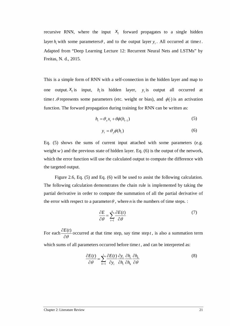
illustrates the LSTM architecture:
Hidden Layer
Inputs tx
ty Outputs
th
0.1)( 1 =−thθφ
Chapter 2: Literature Review 24
Figure 2.8: The architecture of Long Short Term Memory. The Architecture of
memory cell jc and its gate units: input jin and output jout . The self-feedback
connection (with weight 1.0) indicates recursive with a delay of 1 time step, which
forms the basis of the “constant error carrousel” CEC. The gate units function as
open and close access to CEC. Adapted from “Long Short Term Memory” by S.
Hochreiter, 1991.
Input and Output gates are those who learn from all the nonlinear activation
functions before data can be stored in the memory cell (the CEC). From
mathematical point of view, Input and Output gates share the calculation burden
from the memory cell, and the memory cell only performs arithmetic operation. For
instance, g activation function scales the input before Input Gate allows the input
pass into the cell; while h activation function squash the data, and pass Output Gate
before the input is allowed to pass out the memory block. The setup has simplified
the calculation in the whole architecture as each feature takes charge certain
functionality and roles.
Overall, this entire architecture makes long term memory happens. However,
this strength has also “contributed” to a weakness when the cell states tend to grow
linearly in an unbounded manner. This weakness becomes obvious if the input comes
in continuously, and this is not useful when the main reason of using RNN is to deal
with a really long time steps. Therefore, these reasons have led to next consideration
– Forget Gate.
2.1.4.2 The Ability of Forgetting
Forget gate is the later major enhancement to the LSTM architecture that was
developed by Gers in 2001. Forget gate is designed to remove irrelevant information

Chapter 2: Literature Review 25
gradually that are stored in the memory cell. This ability is excellent especially when
performing a huge data analysis in long run. A quick remind from the previous
subsection that based on the following equation:
)( 1−+= ttxt hxh θφθ
(5)
This equation states that the memory cell will grow for every time step, which
implies the memory cell can increase in an infinite manner by default. Indirectly, the
memory cell creates another issue after overcome the problems of vanishing and
exploding. In order to protect its strength, Input and Output gates are invented to
protect the functionality of the memory cell through taking the main responsibility of
learning. In other words, the CEC is only built for storing. Although the original
architecture was not completely ready to use for real-world applications, it owns the
general quality to become the central machine technique for processing all data
types. However, the CEC with Forget gate will form a strong partnership to
overcome the issue of growing infinitely, as the Forget gate learns to remove
unrelated information. In return, the CEC remains its strength for bridging a long
time memory, and Forget gate assists to erase unimportant information gradually.
Another reason Forget gate comes in essence to the project is because the
nature of mathematics and statistics need a way to adapt new information. For
simplicity, Figure 2.9 will be used to assist for explanation. :
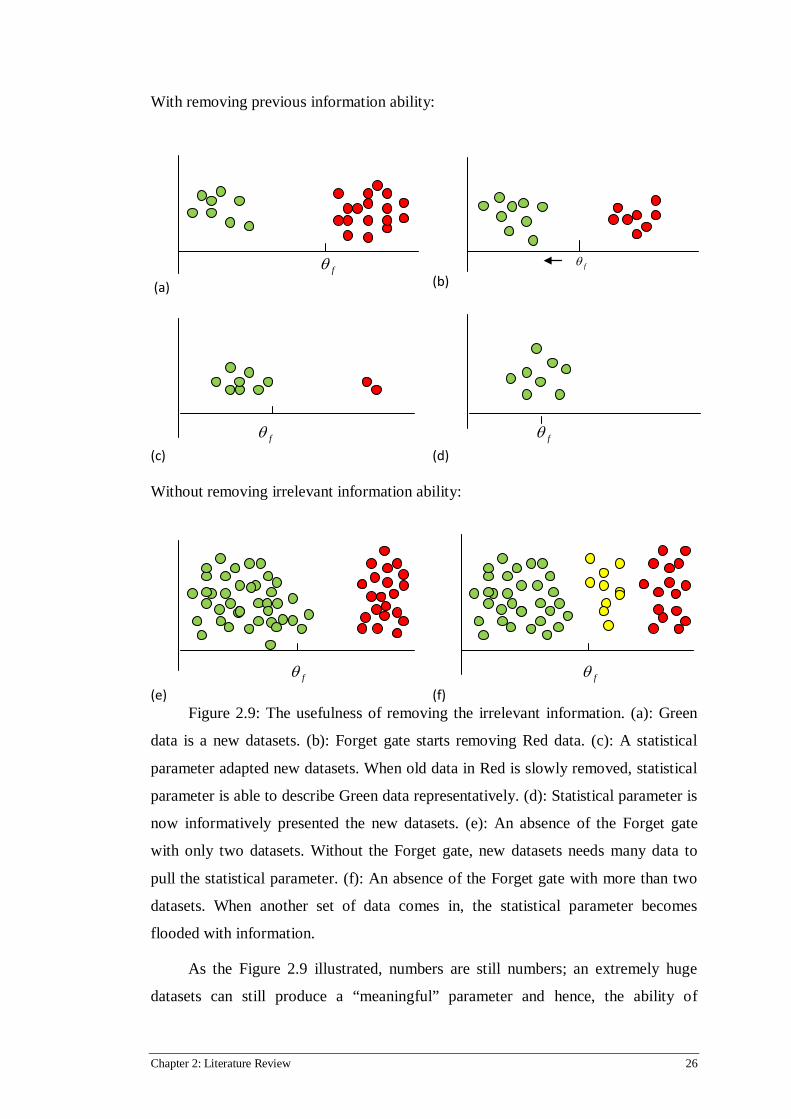
Chapter 2: Literature Review 26
With removing previous information ability:
fθ (a)
fθ (b)
fθ (c)
fθ (d)
Without removing irrelevant information ability:
fθ (e)
fθ (f)
Figure 2.9: The usefulness of removing the irrelevant information. (a): Green
data is a new datasets. (b): Forget gate starts removing Red data. (c): A statistical
parameter adapted new datasets. When old data in Red is slowly removed, statistical
parameter is able to describe Green data representatively. (d): Statistical parameter is
now informatively presented the new datasets. (e): An absence of the Forget gate
with only two datasets. Without the Forget gate, new datasets needs many data to
pull the statistical parameter. (f): An absence of the Forget gate with more than two
datasets. When another set of data comes in, the statistical parameter becomes
flooded with information.
As the Figure 2.9 illustrated, numbers are still numbers; an extremely huge
datasets can still produce a “meaningful” parameter and hence, the ability of

Chapter 2: Literature Review 27
removing the irrelevant data is fundamentally important for mathematics and
statistics, in order to summarise information meaningfully. Similarly, Forget gate
enables the CEC with the ability to reset its memory gradually. Altogether, the
LSTM architecture with the CEC and three gates have provided the basic needs to
perform different tasks’ analyses, especially for real-world applications.
To sum up, the LSTM architecture with Forget gate is a promising Machine
Learning technique. Firstly, the LSTM architecture is designed to overcome the
fundamental problem of Deep Learning, which aims to solve the problem of
vanishing or exploding. In return, the LSTM assists the machine to learn through
many time steps back. Together with Forget gate, the CEC owns an ability to remove
old information. These two attributes are practically useful to deal with big and
highly-correlated datasets, which indirectly reduce the intensive handcrafted feature
engineering. Often, datasets that derived from the real world are presented in many
forms, but one similarity of all the datasets is that they must be occurred
subsequently in an observable manner. An observable manner means that the
patterns of the datasets must be followed one after another in order to be studied.
From this perspective, the LSTM with RNN functionality is highly recommended, as
it is powerful in processing sequential calculation. Therefore, the LSTM architecture
owns the quality to possibly develop into a central machine that learns all kinds of
data such as speech, audio and now image. In particular to this project, the LSTM
will apply on region-based Texture Classification for on-board UAV decision
making during landing.

Chapter 2: Literature Review 28
2.2 TEXTURE FEATURE EXTRACTION
Surface texture gives important information on the solidness of an object, and
allows human to differentiate or appreciate the aesthetic appearance of the objects.
Similarly, surface texture is believed that it can help the UAVs to visually distinguish
areas on the ground and hence, the UAVs land safely.
Texture classification is to design an algorithm for classifying or segmenting
unseen images to a known classifier which have been provided in training examples.
The whole process requires feature extraction and classification as illustrated Figure
2.10. :
Figure 2.10: A general framework to perform texture classification. All imaging
datasets has to go through pre-processing stage before they are ready be classified.
As the main task of this project is to correctly assign labelling to the datasets
based on texture features, it is necessary to have a background understanding on both
input data and pre-processing techniques that use for texture feature extraction. This
is because the understanding of how the texture features are extracted will provide a
better knowledge on data organisation and algorithmic designation. This chapter
briefly discusses the common techniques used in feature extraction, and addresses
the issues of texture representations in general techniques.
2.2.1 The Methods of Feature Extraction
According to Tuceryan and Jain (1993) texture analysis techniques can be
broadly divided into four categories: statistical, geometrical, model-based and signal
processing, which will be briefly discussed as presented following:
Pre-processing
Classification
Objective
Applied Techniques
The Methods of Feature
Extraction
Machine Learning
Techniques

Chapter 2: Literature Review 29
2.2.1.1 Statistical Techniques
Statistical methods use different level of order statistics to compute on the local
features at each point of the image to analyse the spatial distribution of grey values.
The local features are defined by the numbers of pixels are used for computing, for
instance, the first-order statistics focuses the properties (i.e. average and variance) of
single pixel value, but do not consider the spatial interaction between pixels; while
more than first-order statistics estimate covariance between two or more pixels
surrounding.
Statistical approach is one of the well-established methodologies in computer
vision and has been successfully implemented in texture classification; these
techniques include Co-occurrence features (Haralick, Shanmugam, & Dinstein 1973)
and Grey Level Differences (Weszka, Dyer, & Rosenfeld, 1976) which are further
developed into different statistical approaches for later on such as Signed differences
(Ojala, Valkealahti, Oja, & Pietikainen, 2001) and the LBP (Local Binary Pattern)
operator (Ojala, Pietikainen, Harwood, 1996), which incorporates occurrence
statistics of simple local microstructures, thus combining statistical and structural
approaches to texture analysis. Grey-level co-occurrence matrices (GLCM) use
statistical technique to characterise the texture by calculating how frequent pairs of
specific pixel values with specified spatial relationship occur in an image based on
the matrix created by the user (Kubo, & Kadla, 2003). Gabor Wavelet Features is
also another statistical approach that acts very similar to mammalian visual cortical
cells (Marčelja,1980), which found to be useful for texture representation to achieve
optimal coverage in the Fourier domain. The above traditional statistical approaches
to texture analysis such as co-occurrence matrices, second order statistics, GMRF
and local linear transforms are restricted to the analysis of spatial interactions over
relatively small neighbourhoods on a single scale. As a consequence, their
performance is best for the analysis of micro-textures only (e.g., Unser, 1995, p.
1549).
2.2.1.2 Geometric Techniques
Geometrical methods attempt to describe the texture primitives and the rules
governing their spatial organization. The primitives may be extracted by adaptive
region extraction (Tomita, & Tsuji 1990), by edge detection with a Laplacian-of-
Gaussian or difference-of-Gaussian filter (Marr, 1982; Voorhees, & Poggio 1987;
Chapter 2: Literature Review 30
Tuceryan, & Jain 1990), or by mathematical morphology (Matheron, 1967; Serra,
1982). After the primitives have been identified, the analysis will be continued either
by calculating statistics of the primitives (e.g. intensity or orientation) or by breaking
down the placement rule of the elements (Zucker, 1976; Fu 1982).
The structure of the primitives can also be found using Voronoi tessellations
(Ahuja, 1982; Tuceryan, & Jain, 1990). Davis (1979) defined generalized co-
occurrence matrices to describe second-order statistics of edges. The approach was
extended by Dyer and colleagues (1980) to include the grey pixels surround the
edges into the measurement. To look for pairs of edge pixels is another generalized
co-occurrence matrices, which satisfy certain conditions of edge magnitude and
direction. Hong and his colleagues (1982) presumed that edge pixels provide a closed
contour, which primitives can be extracted through searching for edge pixels that
have opposite directions such as, they assumed to be on the opposite sides of the
primitive, followed with a region growing operation. The properties of the primitives
such as area or average intensity can be used as texture features.
Pietikäinen and Rosenfeld (1982) used statistics to measure edge pixels with
pairs that had opposite directions within a defined distance between the pairs. The
result from the calculation was then used as texture features (e.g. distance between
the edge pixels). Regardless, one of the restrictions in the geometric segmentation
methodologies is differential geometry only applies to objects with at least second-
order continuous which images are not always second-order continuous in practice.
As a result, applying this technique would yield poor results around the edges of the
objects (Pieroni, 2013).
2.2.1.3 Model-based Techniques
Model-based methods hypothesize the underlying texture process through
constructing a parametric generative model, which could create the observed
intensity distribution. The intensity function describes the known structural
information on the image surface and an additive random noise sequence.
Generally, an image can be modelled based on either pixels or regions. Pixel-
based model views image as a collection of pixel, which assumes no spatial
interaction between neighbouring pixels, and the observed intensity function is
assumed to be the sum of a deterministic polynomial and additive noise (Haralick &

Chapter 2: Literature Review 31
Watson 1981). Region-based models characterise image as a set of subpatterns, a
classic example is random mosaic models, which fit an image into regions with
specified grey levels to the regions (Schachter, Rosenfeld, & Davis, 1978).
One-dimensional time-series models such as, autoregressive (AR), moving-
average (MA), and autoregressive-moving-average (ARMA), model statistical
relationships of intensities along a raster scan by assuming that noise source is
independent. Another popular technique is Random field models which analyse
spatial variations in two dimensions. For instance, a local Markov random field
models the conditional probability of the intensity for a given pixel depending on the
intensities of the neighbouring pixels.
Mandelbrot (1983) proposed describing images with fractals as a set of self-
similar functions characterized, is known as fractal dimension. The fractal dimension
is correlated to the perceived roughness of image texture (Pentland 1984). In
addition, fractal model has high power in low frequencies, which allows them to
model processes with long periodicities. However, this model is very sensitive to the
size of images. Often, texture in an image is so difficult that similar texture features
can be identified, which makes this interesting model is not suitable for
characterizing the features.
2.2.1.4 Signal Techniques
Signal processing methods analyse the frequency content of the image. Gabor
and Wavelet transforms are widely used in signal processing methods to analyse the
frequency content of the image which use various time-frequency analysis for texture
detection. Gabor functions were extended to two dimensions by Daugman (1985) for
image analysis. Gabor filters were found useful for feature extraction as it functioned
similar to simple cells that found in the visual cortex of mammalian brains
(Daugman, 1985). A major disadvantage in using Gabor transform is that the output
of Gabor filter banks are not mutually orthogonal, which may result in a significant
correlation between texture features. Moreover, these transformations are usually not
reversible, which limits their applicability for texture synthesis. However, wavelet
transform can prevent all mentioned above. As a result, Wavelet function provides a
precise and unifying framework to analyse a signal at different scales (Unser, 1995).
Wavelet transform uses the low pass and high pass filters to remain similar between
two consecutive scales whereas the Gabor approach requires filters of different

Chapter 2: Literature Review 32
parameters (e.g. Chang and Jay Kuo, 1993). Wavelet is a powerful mathematics to
model non-stationary signalling, but other feature extraction methods are still needed
to retrieve features in the next process.
Perhaps, the biggest challenge to these techniques is that, textures in the real
world are not uniform, which often needs to combine many methodologies to extract
textures features meaningfully. In addition, the numeric representations on texture
properties changes as texture changes in orientation, scale or other visual appearance,
and consequently, affecting the choice in image acquisition, sampling and other pre-
processing methods. Therefore, a completely new descriptors and statistics are
unavoidable for the change in viewpoint or surface orientation, which shows as
Figure2.11 (Manik, 2004). :
Figure 2.11: The effect of scale and rotation on textures. On the left, the camera was
moved away from the brick wall. On the right, the surface was rotated in plane by 90
degree while all other imaging conditions were left unchanged. (quoted from Manik)
Adapted from “Statistical Approaches To Texture Classification” by V. Manik,
2004.
Although some techniques attempt to factor in complex scenarios or develop
approaches that are task-specific, there are some other important issues and concerns
are worth to be considered and will be discussed further generally in the following
section.
2.2.2 Limitations and Concerns
One of the major issues brought up in Manik’s thesis (2004) was that, texture
algorithmic designation is sometime caused by the discrimination of the preattentive
visual system, which is based on the density of texture primitives (Julesz, 1981;
Julesz, & Bergen, 1983). This is known from psychophysics and neurobiology.
Programmers are often influenced by psychophysics and neurobiology in order to
design algorithms based on what features should be extracted from images for
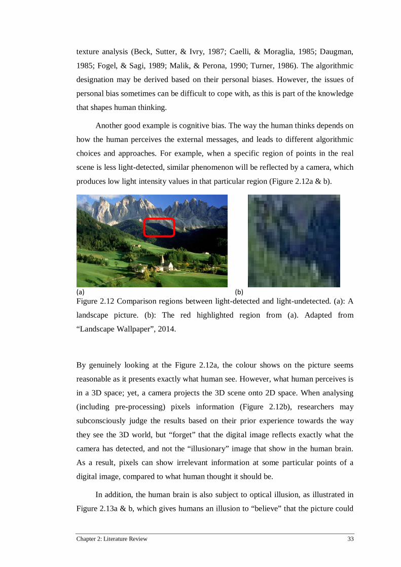
Chapter 2: Literature Review 33
texture analysis (Beck, Sutter, & Ivry, 1987; Caelli, & Moraglia, 1985; Daugman,
1985; Fogel, & Sagi, 1989; Malik, & Perona, 1990; Turner, 1986). The algorithmic
designation may be derived based on their personal biases. However, the issues of
personal bias sometimes can be difficult to cope with, as this is part of the knowledge
that shapes human thinking.
Another good example is cognitive bias. The way the human thinks depends on
how the human perceives the external messages, and leads to different algorithmic
choices and approaches. For example, when a specific region of points in the real
scene is less light-detected, similar phenomenon will be reflected by a camera, which
produces low light intensity values in that particular region (Figure 2.12a & b).
(a)
(b)
Figure 2.12 Comparison regions between light-detected and light-undetected. (a): A
landscape picture. (b): The red highlighted region from (a). Adapted from
“Landscape Wallpaper”, 2014.
By genuinely looking at the Figure 2.12a, the colour shows on the picture seems
reasonable as it presents exactly what human see. However, what human perceives is
in a 3D space; yet, a camera projects the 3D scene onto 2D space. When analysing
(including pre-processing) pixels information (Figure 2.12b), researchers may
subconsciously judge the results based on their prior experience towards the way
they see the 3D world, but “forget” that the digital image reflects exactly what the
camera has detected, and not the “illusionary” image that show in the human brain.
As a result, pixels can show irrelevant information at some particular points of a
digital image, compared to what human thought it should be.
In addition, the human brain is also subject to optical illusion, as illustrated in
Figure 2.13a & b, which gives humans an illusion to “believe” that the picture could

Chapter 2: Literature Review 34
be a solid object by viewing the object from different angles. Thus, designers may
hold biases when designing an approach towards the problems.
(a)
(b)
Figure 2.13.The demonstration of optical illusion. (a) A picture shown at certain
angle (e.g. normal perspective). (b) Viewing (a) from different angle. Adapted from
“35 Insane Optical Illusions That Will Make You Question Your Sanity”, M. Pygas,
(18 July 2015).
The cognitive bias and optical illusion are just the common mistakes that occur while
designing approaches to process imaging datasets. In fact, the understanding behind
the technology of a camera is the key, as it forms the imaging datasets a self-standing
property within them, and this is also a crucial stage to have a clear definition. These
numeric representations obtained from digital images, to some extent, it is just a
bunch of numbers that form its own space, which can be seen as (pure) numbers; on
another extent, this group of numbers carry meaning that reflects information, which
the project defines as “data”. In order to develop a descriptive modelling that can
meaningfully extract texture features, it is essential to briefly understand the sciences
that influence the behaviour of the imaging datasets before reaching the stage of data
organization, although this area will go beyond the scope of the project coverage.
The nature of imaging datasets can be seen as another factor that affects the
way the approaches will be designed. For instance, before “colour” is digitised into a
pixel, the technology of a camera is designed based on the idea of quantum physics;
while pixels on an image sensor are arranged in a manner aimed to suit human
perception. When further tracing the functionality behind the pixels, each pixel
corresponds to the “exact” point of the real scene. This information implies that each
pixel is only responsible to present the brightness and colour information, subject to
the position of the pixel that locates on the image sensor. On the other hand, the
arrangement of the pixels is intentionally organised in a manner that suits the human

Chapter 2: Literature Review 35
brain to visualise. From this reasoning, the connections between pixels seem relevant
in the human world; in fact, the numeric representation of pixels simply reflects the
colour intensity information that is detected by the camera, which the position of
each pixel corresponds to the “exact” point of the actual scene. In short, human
perception is not one of the fundamental factors that numerically change pixels’
information. As a result, this logic explains the stochastic behaviour presents in the
relationship among pixels. Despite that digital images show in the human brain look
smooth and near-flawless by putting millions pixels into a matric form, and this
information implies that objects are possibly traceable through the relevancy between
pixels; the current imaging dataset has not ready yet to perform semantic
classification. Putting this information into an assumption, if a technique processed
the imaging datasets as how the human brain perceives the datasets like a picture,
such as looking connections between pixels, then the techniques may have difficulty
to find a pattern. However, this is just an assumption, to make this assumption as a
solid statement will go beyond the focus of this research, still, the assumption does
come with the rationale which further explain in the future work section.
In addition, colour is another crucial topic that needs to be understood
reasonably well, in order to avoid confusion while approaching the imaging datasets.
The concept of colour is fairly complex as one part of it is about the physical
phenomenon of colour emission, and another part of it is how the human visual
system works. Before these two sides of concepts in terms of colour can be linked
and translated into a digital image, both areas go through many layers of
understanding and studies. For instance, in order to understand the natural
phenomenon of colour emission, it is necessary to understand the properties of light
and go as far as to atomic level, as atoms are the basic structure of most of the
objects. The impact between the light and the atoms contribute to an effect, if this
effect can excite the cones and rods that are detectable by the human eye, and then
the human sees colours. This natural phenomenon is fundamentally important as the
theory behind it argues that, the colour is emitted by an object can only fall in certain
range. This argument indirectly gives an important clue to trace the likelihood of
colour emission; regardless that human may perceive a similar colour differently, due
to colour blind or lighting condition. Importantly, this is how the nature works, and
so the image must provide some kind of information to be based on or linked to.

Chapter 2: Literature Review 36
Then, the colour variation can be traced. This information is very useful when
dealing with the datasets that represents a different time, such as sunset or raining
day. This likelihood of colour emission has assisted the project in later data
designation for the main research application; again, the objective of the project is to
provide a general idea of possible considerations, but the detail of these sciences will
not be relevant to this project. To emphasize, this project has not even touched the
topics on tracing rays, which analyses light source, objects’ (or scene) properties and
viewpoints together.
How a human perceives colours is just the biological part to understand how
the digitized colour is designed and presented. All the digital devices also have their
own properties which the datasets needs to follow and hence, changing the way
information is presented. For instance, in order to produce a colourful digital image
for human usage, each pixel is responsible to produce its colour or brightness
information through adjusting RGB values. For this reason, R, G and B values of
each pixel must be treated together in order to retain pixel’s information. However,
some well-known techniques do not approach the RGB data in this manner.
Certainly, modellings have no right or wrong until objectives are defined. If R, G,
and B are viewed as the carriers of a pixel, by first assigning weight randomly to
each R, G, and B value before treating the values together, this process
mathematically treats R, G, and B values as individual. In return, this process change
semantic meaning carried by each value in R, G, and B for a pixel, subsequently
influence the behaviour on pixel level, and impacting on the whole image analysis. In
short, the RGB values do not behave as its initial role does for the digital image, and
drives the measurement into different analysis. Furthermore, “number” consists its
own meaning. For example, from 1 to 2 is 1 level up in terms of number perspective,
but when “1” and “2” represents information, it is no longer 1 gap difference but
depending on the relationship between information. Although “nonlinear” methods
attempt to explain this scenario, when it comes to the digital environment, the
numeric representation does not just intentionally design to suit human usage, but
also carefully manipulated to fit into the digital devices framework. Indirectly, the
knowledge translated from the sciences of physical phenomenon, biology, digital
data, to numeric representations has created a very different perspective, or universe
that may need further investigation.

Chapter 2: Literature Review 37
Figure 2.14 attempts to demonstrate the process of transforming the datasets
from the natural observation to the digital world, and now human try to use the
digitised dataset for further interpretation.
Natural Phenomenon
“The Bridge” (real-world data translated into digital world)
Further Interpretation
Figure 2.14: The process of transforming data into different space.
This figure attempts to explain the representation of the datasets has also changed
fundamentally along the transforming process, while translating the real-world
collection from the physical phenomenon to the digitized information. Therefore, it
may need to reconsider that not all digital numbers are a ready for statistical
modelling; different layers of digital representation may need entirely different
approaches.
Although all the limitations and concerns discussed here are completely
beyond the coverage of the research objectives, but it is helpful to understand briefly
the shortage and logic behind it. Altogether, this series of understanding have
provided the knowledge on the project about, how to design the datasets by avoiding
the problems of high randomness found in the imaging datasets. Once the issue of
From natural observation to data collection. Samples derived from observations (natural phenomenon) through mathematical modelling.
Data Transformation: “The Bridge” is supported by many concepts of sciences in order to transform real-world information into digital form. (It has also indirectly created another “universe” for sciences to solve.
From digitised data to further interpretation. After great effort of converting analogue signal to digital representation, the digital data is now formed and ready for human usage.

Chapter 2: Literature Review 38
randomness is solved, the question of processing large samples sizes will be
overcome. In addition, by focusing on the property of the imaging datasets, the
cognitive biases will slowly be shifted away as the technique is not built by relying
on the prior knowledge (e.g. how we see a picture), but based on the theory that build
upon the fundamental concepts. In short, by understanding how the property holds in
the dataset, the behaviour of the dataset can be controlled, and organised in a way to
fit into the LSTM algorithm; in fact to all Machine Learning techniques.
To sum up, all techniques that use to extract features do possess advantages
and disadvantages. As numerical representations on texture properties change subject
to the textures in the real world, it is understandable why a few methodologies are
always needed in order to pre-process the imaging data meaningfully, especially
when the texture in the real world can be presented in any forms. Cognitive factors
also play an important role to govern the way the data is organised and the algorithm
is designed. The properties of the imaging datasets are also another essential part to
be understood, as the knowledge will help to organise the data or enhance the
approach. For instance, by understanding how the pixels behave helps to develop a
strategy to move away, as far as possible, from dealing with the datasets in a
connected way, which means not treating pixels in a grouping manner, but
processing one pixel at a time. The properties of imaging datasets also include the
concept of colours that are defined by physical phenomenon, as well as the
representation of datasets that is tranformed from analogue signal to digital
information, which serves as part of the vital grounds to design the imaging datasets
in a meaningful manner.
This brief analysis on the properties of forming the digital images has inspired
us, and understand that different approaches are required to cope with factors such as
light direction, viewpoint, as well as objects’ properties (e.g. opaque); which not DL
techniques alone can perform. However, all data must eventually be able to sample
before carrying to the next level of analysis. Therefore, DL algorithms can apply at
every particular stage to seek for the patterns, as the mathematics used behind DL
techniques is to group statistical modellings together to run autonomously. In order
to develop a solid approach for image analysis, it is necessary to consider the
appropriateness of the modellings for achieving the goal. As the project claims that
DL techniques are formed by a set of statistical modelling, then the first requirement

Chapter 2: Literature Review 39
to use statistical modelling is that the dataset must preserves patterns. Due to the
combinations of RGB numeric representations control colour and brightness
parameters, the RGB intensity values tend to fluctuate greatly. Thus, it is important
to deal with one feature at a time. Since colour information is the most basic
information that can be obtained straight from all colour spaces, colour will be the
first information to be extracted (Brightness information will be dealt by different
approaches that will explain in “Future Work”). For these reasons, we introduce a
different approach - xy Chromaticity Colour Space, to overcome the fluctuating
problem by recognising the pixels’s location, which will be further explained in next
section.

Chapter 2: Literature Review 40
2.3 THE XY CHROMATICITY COLOUR SPACE
Colour is the consequent interaction between light and objects. Colour is the physical
phenomenon of light and also the perception of human brain as shown on Figure
2.14. As a sensation experienced by humans and some animals requires a complex
neurophysiological process, colour is simply the way humans perceive different
types of electromagnetic spectrum within the visible range. The methods used for
colour specification today belong to a technique known as colorimetric and consist of
accurate scientific measurements based on the wavelengths of three primary colours:
Red, Green, and Blue (RGB).
Figure 2.15: Colour is the human perception. Adapted from “Pigments” by The
Pennsylvania State University (18 July 2015).
The intensity values of RGB are the lowest layer of raw numeric representation. In
addition, the digital images are produced based on the adjustment of these RGB
intensity values. As a result, to stabilise the great fluctuation in the RGB intensity
values serves as another key goal in this project, so that the machine can learn
effectively without requiring many samples to derive representative parameters. This
section presents the general background on the xy Chromaticity Colour Space,
demonstrates how the raw RGB datasets is organised as an input for texture
classification, and discusses the advantages of learning pixels’ location in the end of
the section.
Colour Space is a method to specify, create and visualise colours. Different
colour spaces are designed better for particular equipment as well as serving for
different purpose such as more user-friendly than the other. Digitised Images may be

Chapter 2: Literature Review 41
presented in vary Colour Space depending on the devices or situations, importantly;
most of the colour spaces are interchangeable.
CIE 1931 XYZ Colour Space was designed to describe all colours visible to
humans, and it provides a standardised reference against which other colour spaces
are defined. In CIE 1931 XYZ Colour Space, it shows the quantitative links between
wavelengths in the electromagnetic visible spectrum, and the physiological colour
perception in human vision. The mathematical relationships provided from CIE 1931
XYZ Colour Space enable the translation from a human colour vision response to
colour inks, illuminated displays, or recording devices such as digital cameras.
The most useful tool provided by the CIE 1931 XYZ Colour Space to this
project is xy Chromaticity Diagram (or Yxy Colour Space), which describes colours
in two dimensions. This means the xy Chromaticity Diagram allows the RGB values
to be converted into xy coordinate, even though it is not a perfect match and may not
be the best tool; it generally provides a way for the machine algorithm to pick up the
signal in a more effective manner by recognising the pixel location that is defined by
xy Chromaticity Diagram (pixel location in this colour space). The main idea of
learning the pixel location aims to avoid processing the great variance in the RGB
values. Once the RGB numbers are settled, the pattern can be presented. Therefore,
small samples of images are sufficient to be analysed. Figure 2.16 shows an example
of a different lighting condition can bring a complete numeric representation of the
RGB values. However, the method of recognising the pixels’ location that is
specified by xy Chromaticity Diagram will largely reduce the difficulty to search for
the patterns in this scenario, which will explain further later on. :
(a)
(b)
Figure 2.16: The datasets depends on lighting condition. (a) A better
lighting condition picture. (b) A poorer lighting condition picture. The
datasets highly subject to the lighting condition change as the datasets

Chapter 2: Literature Review 42
only presents lighting and colour information. Adapted from “xstitch”
by Ratter, 2012.
Another useful information provided from xy Chromaticity Diagram is that the
quantitative links to the wavelengths of the electromagnetic visible spectrum. This
information allows the datasets to be further analysed in terms of the likelihood of
colour range that an object will produce subject to the direction of the light.
Certainly, this approach will blend into physics-based analysis, which requires
another research.
From algorithmic point of view, xy Chromaticity Diagram has also simplified
the tasks of defining a threshold to represent a colour. Indeed, using colour as
learning input to predict another dataset is statistically demanding. Apart from the
reasons that colour changes due to many factors (e.g. objects’ properties:
translucent), defining colours is also algorithmically challenging as some colours are
formed by the convolution of wavelengths. Although many sophisticated modellings
developed to distinguish colours as close as possible, the step of defining colours is
like attempting to segregate water and oil problem. In addition, numbers are still
numbers; the modellings have no “idea” what are the inputs but searching to
converge. This reason also explains why some parameters are misleading as
“descriptive” parameters can be derived through extremely huge dataset. To answer
these series of questions, xy Chromaticity Colour Space is suggested, to overcome
the fluctuating problem by recognising the pixels’s location (grid that is defined by
xy Chromaticity Diagram), as well as suggesting a straightforward method to define
colour.

Chapter 2: Literature Review 43
Figure 2.17 briefly demonstrates the RGB pixels in an image projects onto the 2D
colour space, the xy Chromaticity Diagram.
(a)
(b)
(c)
Figure 2.17: The colour spaces conversion between the RGB values to the xy
Chromaticity. (a) An image to be represented in xy. (b) The RGB Colour Space. (c)
The xy Chromaticity Colour Space. Each image is formed by the RGB intensity
values. Each pixel is a representation in the RGB Colour Space which attempts to
show by the lines which links between an image and the RGB Colour Space. The
values in the RGB will then project onto a 2D space, xy Chromaticity Diagram to
stabilize a great change in the RGB intensity values through recognising the pixels
location that fall onto. That particular region that highlighted by the red circle will
assist the machine algorithm to recognise the pixels patterns. Figure (a) Adapted
from “Oack Tree PNG Clipart Picture” by Gallery Yopriceville, 2015. Figure (b)
Adapted from “How Punjabi, the Gurnukhi Language and Grammar Systems” by H.
Singh, 2014. Figure (c) Adapted from “Colour Perception” by C. Cauwerts, n.d.
The following example attempts to give a closer understanding how the
intensity values move greatly in the RGB colour space, despite that they produce a
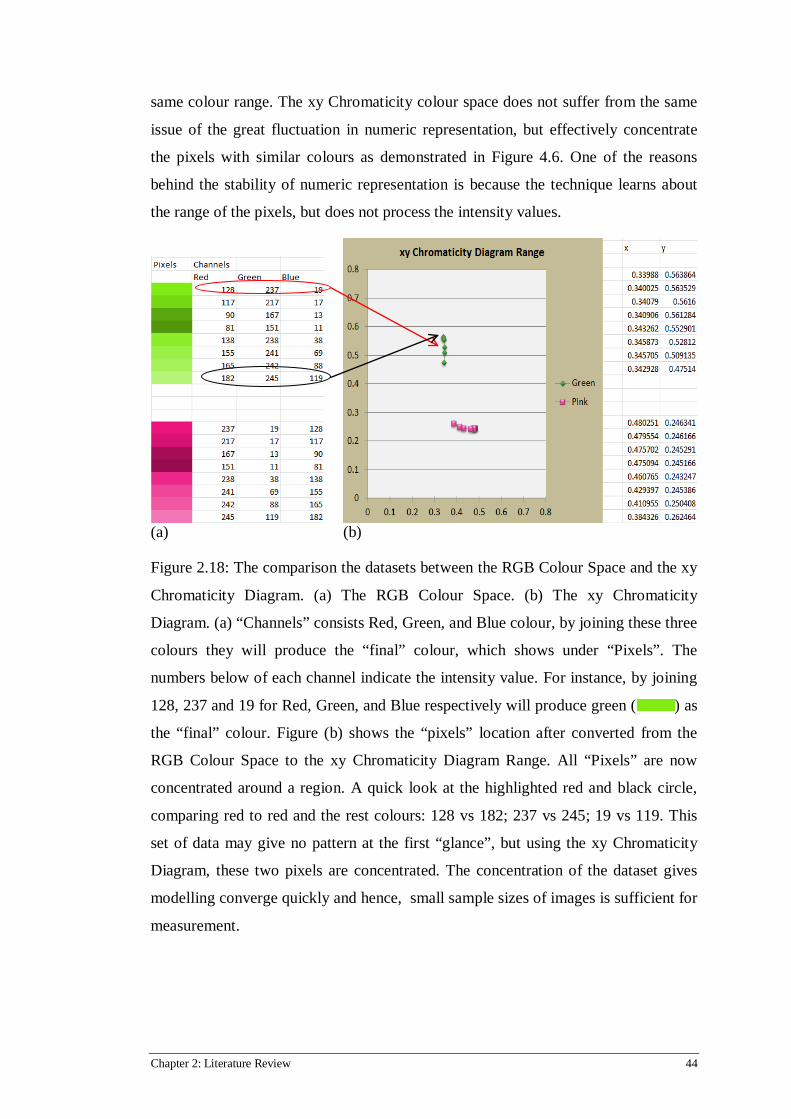
Chapter 2: Literature Review 44
same colour range. The xy Chromaticity colour space does not suffer from the same
issue of the great fluctuation in numeric representation, but effectively concentrate
the pixels with similar colours as demonstrated in Figure 4.6. One of the reasons
behind the stability of numeric representation is because the technique learns about
the range of the pixels, but does not process the intensity values.
(a)
(b)
Figure 2.18: The comparison the datasets between the RGB Colour Space and the xy
Chromaticity Diagram. (a) The RGB Colour Space. (b) The xy Chromaticity
Diagram. (a) “Channels” consists Red, Green, and Blue colour, by joining these three
colours they will produce the “final” colour, which shows under “Pixels”. The
numbers below of each channel indicate the intensity value. For instance, by joining
128, 237 and 19 for Red, Green, and Blue respectively will produce green ( ) as
the “final” colour. Figure (b) shows the “pixels” location after converted from the
RGB Colour Space to the xy Chromaticity Diagram Range. All “Pixels” are now
concentrated around a region. A quick look at the highlighted red and black circle,
comparing red to red and the rest colours: 128 vs 182; 237 vs 245; 19 vs 119. This
set of data may give no pattern at the first “glance”, but using the xy Chromaticity
Diagram, these two pixels are concentrated. The concentration of the dataset gives
modelling converge quickly and hence, small sample sizes of images is sufficient for
measurement.

Chapter 2: Literature Review 45
The advantages of learning the pixel’s location are:
1. Arranged colours in a more sensible manner without largely depending
on the RGB integers.
2. Simplified the complex information of pixels (e.g. illuminance).
3. Eased of programming and computing architecture designation.
4. Stabilised the learning process as statistical modelling needs a stable
datasets.
With the help of xy Chromaticity Diagram, many existing issues could be
temporarily solved at this stage. For instance, by analysing the locations of the
pixels, it gives mathematical and statistical models reach equilibrium quicker, or
parameters come to an average rapidly with small sample sizes. Also, pixels do not
behave randomly while summarising its locations. Perhaps, colours spaces with more
than 2-dimensional descriptors will introduce many more new calculations to the
entire architecture, which can “confuse” or delay the Machine Learning process. As a
result, the well-defined xy coordinates diagram will help mathematical models learn
to recognise the colours based on the grid defined in xy Chromaticity. Importantly,
the imaging datasets now nicely fits into the Long Short Term Memory architecture.
2.4 SUMMARY
In the literature review, the relevant scopes of Machine Learning techniques
and the imaging datasets are generally covered in order to achieve the research
objectives. The main objective of Machine Learning sections aims to provide the
reasoning why deep recurrent neural network is favoured, particularly that the nature
of recurrent neural network owns the quality of becoming the central Machine
Learning technique, for many real-world applications across different types of
datasets. The Long Short Term Memory is a class of recurrent neural network which
functions as a digital memory chip, together with read, write and reset features.
These features provide the basic needs allowing a highly-correlated datasets is being
analysed continuously.
The main objective of analysing imaging data aims to construct a meaningful
deep modelling. However, we found many inconsistencies when interpreting the
imaging data. Indeed, all Machine Learning techniques need is a pattern, when the

Chapter 2: Literature Review 46
datasets could not or provide no patterns; all Machine Learning techniques will be
struggling, and the concept of Deep Learning will “forever” deep. Unfortunately,
pixels behave no pattern often complicates the Machine Learning techniques in order
to disentangle the information within the datasets. Although the aim of this project
does not focus on the sciences behind the imaging datasets, a basic understanding on
the fundamental concepts that help to form the imaging datasets is provided, in order
to understand the natural behaviour behind the imaging datasets.
The subsection of Limitations and Concerns generally presents the issues while
designing algorithm or creating datasets. A relevant knowledge is provided in order
to understand how the behaviour of imaging data can be stabilised and hence, small
sample sizes of imaging datasets will sufficient to perform analysis. Overall, perhaps
it is worth to re-consider whether the information provided from the digital images
can be modelled by statistical approaches. However, this consideration will leave it
to the choice of preference and beyond the project coverage.
In conclusion, we perceive that the Long Short Term Memory architecture
fulfils overall requirements made by the project, especially the potential ability for
different data types’ analyses. xy Chromaticity Diagram will be used as the texture
feature extraction technique, to stabilise the imaging datasets before it classified by
the LSTM. Eventually, the findings will be used to perform texture classification to
assist the UAVs to perform emergency landing.

Chapter 3: The Long Short Term Memory 47
Chapter 3: The Long Short Term Memory
In principle, Recurrent Neural Networks use their feedback connection as a
form of short-term memory to learn to map between input and output sequences.
This is potentially powerful from the mathematical perspective as the network can
perform intelligently due to its internal state (short-term memory), is being able to
store and wait to learn the target signals from the incoming input. This concept is
appealing to sequential data, especially to applications with time dependence.
Unfortunately, the traditional RNN architecture is only theoretical feasible as it
struggled to learn tasks in short times, with actual delays of more than 10 time steps
between relevant input and target events (Hochreiter et al., 2001). The following
figure provides an overview of the vanishing and exploiting problems for RNN. This
drawback was also the main reason that the standard RNN architecture could not
learn in practice.
Figure 3.1: Vanishing gradient problem for RNNs. The shading of the nodes
indicates the sensitivity of the network to the input at that time (the darker the shade,
the greater the sensitivity). The sensitivity decays exponentially as time pass and new
inputs overwrite the activation of hidden unit and the network ‘forgets’ the first
input. Adapted from “Supervised Sequence Labelling” by A. Graves, 2007.
Long Short Term Memory (LSTM) was first introduced by Hochreiter and
Schmidhuber in 1997 to overcome the vanishing and exploding problems

Chapter 3: The Long Short Term Memory 48
(Hochreiter, 1991). Gers (2003) added on a few important features such as Forget
Gate, to enhance the LSTM, which now serves as the basic structure of the LSTM
architecture. Figure 3.2 demonstrates the LSTM preserves information over time. :
Figure 3.2: Preservation of gradient information by LSTM. The shade of the
nodes indicates the sensitivity of the network to the input at that time. With the
design of the LSTM, the information is now able to be stored across time steps. The
main reasons enables the LSTM learns through many times steps are due to gates
adjustment as displayed either entirely open (‘o’) or close (‘–’). Adapted from
“Supervised Sequence Labelling” by A. Graves, 2007.
At the “Hidden Layer”, each unit (circle) at different time step contains input,
forget and output gates. Input gate shows at the bottom of each unit (connects
between Input and Hidden layer), forget gate is attached with every unit on the left
(self-looping within its attached unit), and output gate locates on top of the unit
(connects between Hidden and Output Layer). The memory cell keeps the first input
as long as the forget gate is open and the input gate is closed. The sensitivity of the
output layer can be switched on and off by the output gate without affecting the cell.
This chapter reviews the main RNN architecture used in this thesis – Long
Short Term Memory. Section 3.1 describes the basic architecture of LSTM. Section
3.2 provides the latest used equations required to train and activate LSTM networks
(In this project, Gers’s (2003) algorithm and equations will be used).

Chapter 3: The Long Short Term Memory 49
3.1 THE LSTM ARCHITECTURE
Long Short Term Memory is an acyclic neural network and the main difference
from the standard RNN is that it consists of a set of feedback connected subnets,
known as memory blocks. Graves (2007) explains that these blocks can be viewed as
a memory chips in a digital computer. Each block can have both one or more
memory cells, and three multiplicative units: input gate, output gate, and forget gate,
that provide write, read and reset operation for the cell(s). The cell is also known as
the Constant Error Carrousel (CEC) and can only be accessed by these three gates
but not the entire network. In other words, the memory cell is the core of the LSTM
architecture in order to keep the information for long times, while the gates are the
key to protect the memory cell(s) with each gate having its own functionality.
Two issues were invoked when designing the CEC, which were the input and
output weight conflict. These conflicts happened because the CEC is not only
connected to itself but also to other units. This means that the same incoming weight
may be used for storing and ignoring signals, where the weight sharing will make
learning difficult, similar happens to the outgoing weight. Therefore, Input and
Output gates are designed to split the job, leave the Input gate and Output gate to
decide what information should be taken inside and outside the block, as well as
communicating with the CEC via the multiplicative units (Figure 3.3: dark blue
circle).
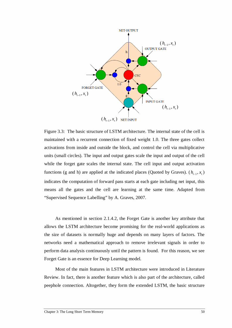
Chapter 3: The Long Short Term Memory 50
Figure 3.3: The basic structure of LSTM architecture. The internal state of the cell is
maintained with a recurrent connection of fixed weight 1.0. The three gates collect
activations from inside and outside the block, and control the cell via multiplicative
units (small circles). The input and output gates scale the input and output of the cell
while the forget gate scales the internal state. The cell input and output activation
functions (g and h) are applied at the indicated places (Quoted by Graves). ( 1−th , tx )
indicates the computation of forward pass starts at each gate including net input, this
means all the gates and the cell are learning at the same time. Adapted from
“Supervised Sequence Labelling” by A. Graves, 2007.
As mentioned in section 2.1.4.2, the Forget Gate is another key attribute that
allows the LSTM architecture become promising for the real-world applications as
the size of datasets is normally huge and depends on many layers of factors. The
networks need a mathematical approach to remove irrelevant signals in order to
perform data analysis continuously until the pattern is found. For this reason, we see
Forget Gate is an essence for Deep Learning model.
Most of the main features in LSTM architecture were introduced in Literature
Review. In fact, there is another feature which is also part of the architecture, called
peephole connection. Altogether, they form the extended LSTM, the basic structure
( 1−th , tx )
( 1−th , tx )
( 1−th , tx )
( 1−th , tx )

Chapter 3: The Long Short Term Memory 51
of memory block with one cell, shows in the Figure 3.3, where the arrows point from
the CEC to the gates is the peephole connection.
3.1.1 Peephole Connection
The functionality of peephole connections is to provide a direct communication
pipeline between the CEC and all the gates. The idea behind peephole connection is
to assist the network to learn precise timings. Although this attribute is an optional
feature to the LSTM architecture, to some extent; this concept is considerably a high
level of intelligence. This is because peephole connections aim at enabling the
network to act ahead based on the numbers of patterns repetitions within a certain
time interval. For example, a pianist knows the rhythmic sequences and will act
precisely at the right time pressing on the keyboards. The intention of peephole
connection is to perform the similar job, which means the network knows ahead. In
other words, the network learns to pick up the critical moment right before the next
information happens, and this is all about timing, which peephole connection aims to
provide.
Indeed, peephole connection is a useful attribute; however, there are many
other enhancements that need to be done before this feature can provide meaningful
results. As a result, we perceive that this attribute is an optional feature at this point
in time, and will be further explained at the end of the thesis. Next section provides
the mathematical representations used to calculate the activation functions and
backward propagation for the LSTM.
3.2 THE LSTM FORWARD AND BACKWARD PASS EQUATIONS
The original LSTM training algorithm (Hochreiter et al., 1997) was an
approximate gradient-based learner, which was calculated by combining Real Time
Recurrent Learning (RTRL; Robinson and Fallside, 1987) and Backpropagation
Through Time (BPTT; Williams and Zipser, 1995). In fact, the exact error gradient is
achievable using only BPTT approach. This section will present the latest version of
forward and backward pass equations (Graves and Schmidhuber, 2005b). The
objective of this section is to provide quick and clear information on the latest
version of the LSTM performing forward and backward propagation. For simplicity,
all the mathematical representation will be similar to Graves’s version (see Grave’s

Chapter 3: The Long Short Term Memory 52
PhD thesis for details). The LSTM equations only present a single memory block.
For multiple blocks the calculations simply repeats for each block.
Let ijw be the weight of the connection from unit i to unit j . The network input
to some unit j at time t is denoted tja and the value of the same unit after the
activation function has been applied is tjb . The subscriptsι , φ and ω refer to the
input gate, forget gate and output gate respectively. The subscript c refers to one of
the C memory cells. tcs is the state of cell c at time t . f is the activation function of
the gates, and g and h are respectively the cell input and output activation functions.
Let I be the number of inputs, K be the number of outputs and H be the
number of cells in the hidden layer. Note that only the cell outputs tcb are connected
to the other blocks in the layer. The rest of the LSTM activations, such as the states,
are only visible within the block. The index h is used to refer to cell outputs from
other blocks in the hidden layer.
Like the standard RNNs the forward pass is calculated for a length T input
sequence x by starting at 1=t , and recursively applying the update equations while
incrementing t ; while the BPTT backward pass starts at t = T, and decrementing t at
each time step while recursively calculating the unit derivatives. The final weight
derivatives are found by summing over the derivatives at each time step, which
expresses as:
∑∑==
=∂
∂
∂∂
=∂∂ T
t
ti
tj
T
t ij
tj
tjij
bwa
aO
wO
11δ
(12)
where tj
tj a
O∂∂
=δ and O is the objective function used for training. For simplicity,
Figure 3.4 shows as reference for forward pass calculation (Note: the figure will use
together with Forward Pass Equations).

Chapter 3: The Long Short Term Memory 53
Figure 3.4: This Figure shows as reference for forward pass calculation. Input
data, tix , starts accepting at four different points: Net Input, Input, Forget and Output
Gate. Each of the point has recurrent in the hidden layer H . Input, Forget and Output
Gate, each connects with the cell, called peephole connection C (the arrows point out
from the CEC). The input layer, hidden layer, and output layer will be summed up
and squash by )(⋅f . All the dark blue circles indicate the meeting point between
Input gate & Net Input = )( tc
t agbι , Forget Gate & CEC = 1−tc
t sbφ , CEC & Output
Gate = )( tc
t shbω . Adapted from “Supervised Sequence Labelling” by A. Graves, 2007.
As the LSTM architecture accepts the input at four different points, for
simplicity, the order of the equations present should proceed as specified below,
which is important to perform the forward and backward passes. All states and
activations are set to zero at 0=t , and all δ terms are zero at 1+=Tt . As mentioned,
the Figure 3.4 will help to understand the following formulas (see the Graves’s PhD
thesis for detailed).
taι
tbι
taω
taφ
tca
)( tcag
tcb
tbφ tcs
tbω

Chapter 3: The Long Short Term Memory 54
Forward Pass:
Input Gates:
∑∑∑=
−
=
−
=
++=C
c
tcc
H
h
thh
I
i
tii
t swbwxwa1
1
1
1
1ιιιι
(13)
)( tt afb ιι = (14)
Forget Gates:
∑∑∑=
−
=
−
=
++=C
c
tcc
H
h
thh
I
i
tii
t swbwxwa1
1
1
1
1φφφφ
(15)
)( tt afb φφ = (16)
Cells:
∑∑=
−
=
+=H
h
thhc
I
i
tiic
tc bwxwa
1
1
1
(17)
)(1 tc
ttc
ttc agbsbs ιφ += −
(18)
Output Gates:
∑∑∑==
−
=
++=C
c
tcc
H
h
thh
I
i
tii
t swbwxwa11
1
1ωωωω
(19)
)( tt afb ωω = (20)
Cell Outputs:
)( tc
ttc shbb ω=
(21)

Chapter 3: The Long Short Term Memory 55
Backward Pass:
tcε = error for Cell Output. t
c
tc b
O∂∂
=ε (22)
tcε = error for Cell. t
c
ts s
O∂∂
=ε (23)
Cell Outputs:
∑∑=
+
=
+=H
h
thhc
K
k
tkck
tc ww
1
1
1δδε
(24)
Output Gates:
∑=
=C
c
tc
tc
tt shaf1
)()(' εδ ωω (25)
States:
11111)(' +++++ ++++= tc
tc
tc
ts
ttc
tc
tts wwwbshb ωωφφιιφω δδδεεε (26)
Cells:
ts
tc
ttc agb εδ ι )('= (27)
Forget Gates:
∑=
−=C
c
ts
tc
tt saf1
1)(' εδ φφ (28)
Input Gates:
∑=
=C
c
ts
tc
tt agaf1
)()(' εδ ιι (29)

Chapter 3: The Long Short Term Memory 56
3.3 SUMMARY
The chapter of Long Short Term Memory generally describes the features that
form the LSTM architecture. The functionality of each feature is also briefly
discussed, particularly peephole connection. Peephole connection can be perceived
as a highly-intelligent attribute as it aims to enable the network responses ahead
before completing the analysis of a stream of data input. However, due to many other
areas are needed to improve before this feature becomes useful, this attribute does
not bring up as a focus. The aim of providing the latest version of the LSTM
equations is to provide a clear understanding on how the LSTM performs forward
and backward pass calculations.

Chapter 4: Experimental Design 57
Chapter 4: Experimental Design
4.1 PROBLEM BACKGROUND
The main application of this research is to perform the final site selection
criterion - Texture Classification Layer for emergency landing, as shown in Figure
4.1.
Figure 4.1: The chart flow of final site selection for emergency landing. Adapted
from “Classifying natural aerial scenery for autonomous aircraft emergency landing”
by L. Mejias, 2014.
In our problem, surface textures are the images (datasets) that represent the
terrain underneath the aircraft. The datasets are categorised into Bitumen, Building,
Trees, Grass, and Water. These data types are important to prioritise suitable areas
for an aircraft to land urgently. Previous work has looked into size, shape or slope
attributes to localise the suitable landing site, one of the possible results from the
previous work is demonstrated on Figure 4.2. :

Chapter 4: Experimental Design 58
Figure 4.2: The output of the candidate landing site selection. Red contour indicates
the possible landing areas. Adapted from “Classifying natural aerial scenery for
autonomous aircraft emergency landing” by L. Mejias, 2014.
Previous research have also attempted to use Machine Learning techniques
such as multi-class Support Vector Machines (SVM) to approach the classification
problem, but from different perspectives. For instance, the former research focused
on classification problem through the use of any tools, and in their case is multi-class
SVM; while this project focuses on a specific tool that can perform any problems,
and in our case is classification. Secondly, both project used very different
architectures to perform measurement, which results may need more information
such as how features are extracted, in order to make a useful comparison and
interpretation. For these reasons, this project does not directly compare with the
previous result (see Mejias, 2014 for results details).

Chapter 4: Experimental Design 59
4.2 DATASETS BACKGROUND
All datasets are aerial images taken from an on-board UAV. There are 2 datasets
provides to this thesis, which will be presented as following.
4.2.1 Dataset 1
Dataset 1 consists the total of 7632 sub-images (with 50-by-50 resolutions of
each sample in order to facilitate the comparison with previous work), and each sub-
image comes with a label or class. 5 classes are available: Bitumen, Building, Grass,
Trees, and Water. The term “sub-image” indicates a sample which originally was a
part or region of a whole picture. For instance, an image with 300-by-300 resolutions
can be divided into 36 numbers of samples (each sample is 50-by-50 resolution).
Apart from the total samples and label attaches with each sample, all information is
unknown for Dataset 1. The following Table 4.1 provides brief information of the
Dataset 1:
Class: Total numbers of available Samples:
An example of 50-by-50 image:
Bitumen 330
Building 438
Grass 3158
Trees 676
Water 3030
Table 4.1: Dataset 1

Chapter 4: Experimental Design 60
Table 4.1: Dataset 1. “Class” indicates labelling. Each label has different
numbers of samples, and make up the total numbers of 7632 samples. A sample is
also shown for better understanding on how the dataset looks like.
4.2.2 Dataset 2
Dataset 2 consists of the total 7 full aerial images with the total of 1740
samples. The differences between Dataset 1 and 2 are labelling and sample division.
The labelling for sub-images in Dataset 2 is defined by the project manually. The
criteria of defining label will be further discussed in the relevant Experiments. Each
sample is retrieved by dividing a full image. As each full image has different
resolutions, also for simplicity, some extra information is excluded in the
measurement. For instance, an image with resolutions of 1076*649 will give 300
total numbers of samples with 50-by-50 resolutions, instead of 314 to simplify
measurement. Dataset 2 is treated as the real application, because the project has
more information about the samples. For instance, each sample is known where it is
retrieved or how label is defined. The following Table 4.2 provides brief information
of the Dataset 2 for all 7 full images:

Chapter 4: Experimental Design 61
Image No. & Resolutions: Total numbers of divided Samples:
Image:
1. 1024*768 300
2. 1024*768 300
3. 768*649 180
4. 1024*768 300
5. 1024*768 300
6. 768*649 180
7. 768*649 180
Table 4.1: Dataset 2

Chapter 4: Experimental Design 62
The following Figure 4.3 demonstrates how each full image is divided into
samples. Class assignation will be explained specifically on relevant experiments.
(a)
(b)
Figure 4.3: An image is divided into sub-images. Figure 4.3a is an aerial full image.
Figure 4.3b shows a sample is retrieved from a full image. Each sample is a 50-by-50
sub-image.
4.3 DATA ORGANIZATION
This section provides an overview on how data is first accepted by the LSTM
architecture and hence, affecting the way data is organised and the choice of
experiments.
4.3.1 How the LSTM architecture processes data
As the LSTM architecture layout is designed for sequential processing, many
problems choose to use the LSTM due to its “dependent” inheritance. However, it is
not always the case. The point is modelling has no idea what they are designed for;
all they “know” is searching for equilibrium (e.g. convergence or pattern). For this
reason, there are many tricks to use a modelling as mentioned in the Literature
Review; “dependent” can be presented in example-based or pattern-based; as long as
data is constructed to suit the modelling behaviour.
To demonstrate how the LSTM sequential measurement can be linked to
classification, the following Figure 4.4 shows a Reber Grammar data organization,

Chapter 4: Experimental Design 63
which will assist to explain how the LSTM processes and result interpretation (see
Herta, 2014 for details of Reber Grammar example).
. . . 1 0 0 0 0 0 0 0 1 1 0 0 0 0 0 0 1 0 0 0 0 1 0 0 0 0 0 0 1 0 0 0 0 0 0 0 1 1 0 0 0 0 0 0 1 0 0 0 0 0 1 0 0 0 1 0 0 0 0 0 0 1 0 0 0 1 0 0 1 0 0 0 1 0 0 0 0 0 0 0 1 1 0 0 0 0 0 0 1 0 0 0 1 0 0 0 1 0 0 1 0 0 0 0 0 0 1 0 0 0 1 0 0 1 0 0 0 0 0 0 1 0 0 0 1 0 0 1 0 0 0 0 0 0 1 0 0 0 1 0 0 0 0 0 0 1 0 0 0 1 0 0 1 0 0 0 1 0 0 0 0 0 0 0 1 1 0 0 0 0 0 0 1 0 0 0 1 0 0 0 1 0 0 0 0 0 0 1 0 0 0 1 0 0 1 0 0 0 0 0 0 1 0 0 0 0 0 0 0 1 0 0 0 0 0 0 1 0 0 1 0 0 0 0 0 0 1 0 0 0 0 0 0 0 0 0 0 1 . . . (a) The flow of data within the LSTM architecture:
(b) Result from the LSTM 0 0 0 0 0 1 0 0 0 1 0 0 1 0 (0.0515)(0.0230)(0.7945)(0.0588)(0.0605)(0.5318)(0.2401) (c)
Space between 2 sequences: The LSTM architecture (Ger’s version) recognises a complete sequence based on a space.
Input or current state
Target or next state
An element of a vector: Each element represents a character defined by Reber Grammar.
Spaces between input and target: The LSTM architecture (Ger’s version) differentiates input and target based on 3 spaces.
0 0 0 0 0 1 0 0 0 1 0 0 1
Forward pass: Backwardpass:
Current State Next State Prediction for Next State

Chapter 4: Experimental Design 64
Figure 4.4: The demonstration of data flow win the LSTM architecture with the use
of Reber Grammar example. (a) The presentation of a complete “sequence”, and
there are many numbers of a complete sequence within a text file. (b) The
demonstration of how the LSTM accepts input and target data. (c) The presentation
of predicted result produced by the LSTM.
Figure 4.4 shows the example of Reber Grammar data organization and result
presentation. Figure 4.4a shows how data is being structured a complete “sequence”,
and there are many numbers of a complete sequence within a text file. To help
algorithm distinguishes 2 different whole sequences, user has to place a “space”
between sequences. Within a sequence, there are different numbers of rows, which
indicates the numbers of steps to complete a sequence. For Reber Grammar example,
each row contains current (input) and next (target) state, and each current and next
state consists of 7 elements to represent 7 different characters.
Figure 4.4b shows how the LSTM accepts the input and target data. Forward
pass indicates the LSTM first processes the input data before it reaches to the
backward pass. As arrows point, when an input arrives at a particular block with one
cell, all gates and the cell (to be clear: net input) are the core processors to receive
input. In other words, the first processing layer begins at four different places. Each
gate will assign weight randomly to each element of the input (see Chapter 3:
forward pass: equations 13, 15, 17 and 19 for details) before error is traced. Error is
traced with the help of supervised learning method as demonstrated by the backward
pass arrow before the final measurement is output by the block tcb (assuming there is
only one cell per block), which connects to the entire Network. Each element from
the target vector will start measuring its difference one element at a time, and final
result can be showed at Figure 4.4c.
Figure 4.4c provides the prediction of the LSTM. “Prediction for Next State”
presents the probability of next state for each character. “0.7945” indicates that the
3rd character has a “0.7945” chance to happen, from probabilistic perspective, any
prediction beyond 0.49, considers as “1”. For example, “0.2401” will classify as “0”,
which gives exactly the target presented. As demonstrated, the probability of “Next
State” is all well-predicted.

Chapter 4: Experimental Design 65
To summarise the information given by Figure 4.4a, b, & c, one important
notice is as the target data is processed one element at a time, the final output
obtained from the LSTM can be seen as classification. This is because the
measurement does not compress all target data in one time processing and hence, the
information presented in the input is preserved for each element of the target.
Another important notice is that “net output” tcb . In order to communicate with the
entire Network, first must bypass tcb which is the only way for the Network to access
a calculated result for that particular block. In other words, whether a row is relevant
to the next or previous row within a complete sequence is the measurement of the
entire network, which will blend into machine learning analysis (e.g. sigmoid
function or learning rate) and is not the focus for this project.
This analysis has lent the project an idea that this scenario is translatable into
classification problem. As there is no start and end point for sub-image classification
problem, the orders of sub-images can be shuffled and presented by one matrix, as
long as it is traceable where the sub-images are originally retrieved from. However,
all the similar classes must be grouped together in order to minimise the MSE. As
mentioned, whether a row is relevant to another row it depends on the Network
measurement, MSE is not relevant to classification problem to certain degree; yet, it
provides a first glance whether the data preserves pattern. For instance, a small MSE
value indicates the Network converged to its minima, which reflects the behaviour of
the dataset. In short, MSE reflects the architecture measurement. Figure 4.5 presents
all sub-images are organised according to the types of classes, and will briefly
explain how the organization brings impact on MSE.

Chapter 4: Experimental Design 66
Figure 4.5: An example of sub-images organization.
In a matrix, each row represents a sample with input and target (class). Within
an input, all elements represent the pixel’s locations that are defined by xy
Chromaticity Diagram (as shown on Figure 4.6); while each element of target
represents a class, which will be further explained in the following section. Orange
highlight indicates a range that is a change from one type of class representation to
another. This particular change will increase MSE as the architecture is adapting
new information. However, this adaption brings an insignificant impact on the final
result as presented on Figure 4.4c.

Chapter 4: Experimental Design 67
4.4 THE STEPS OF CREATING DATASETS
1. These datasets will go through mathematical transformation to XYZ
colour space before xy Chromaticity Diagram is derived (formulas are
provided in Appendix A).
2. After gone through matrix transformation, all pixels are now able to
locate its xy coordinates (will be presented on Appendix A).
3. Datasets will be converted into sequence through counting the
occurrence of pixels that fall in a grid, which is that are defined by xy
Chromaticity Diagram, turn it into binary code (calculation flow will be
demonstrated on Appendix A) and serve as input data.
4. The targeted data is the class types, they are: BITUMEN, BUILDING,
GRASS, TREES, and WATER. (numeric representation of class types
will be given on Appendix A).
5. Input and targeted data will finally combine together and form a big
matrix which each row represents a 50-by-50 image and its class type
(the final data arrangement will be shown on Appendix A). The datasets
is now ready to be classified.

Chapter 4: Experimental Design 68
Figure 4.6 is provided to visualise the steps of creating datasets. For simplicity,
the process of creating dataset will be explained based on the following Figure 4.4.
All images are used in this project is presented in RGB colour space. On Figure 4.4,
image (a) is a digital image, which all its pixels contains RGB information as
pointing from (a) to (b). Each pixel of an image will be converted into xy
Chromaticity Diagram through the descriptions of step 1. Once step 1 has performed,
all pixels are now presented in x and y coordinates which can be seen by following
the arrows point from (b) to (c). As noted, all arrows point to a grid which
highlighted by red circle. All these grids represent its own range, and each range or
grid will be served as algorithmic condition. Algorithm will count the occurrence of
pixels based on each range, and stored in a vector. In other words, each element of a
vector represents a grid. After counted, a vector represents a sample will be formed
which is shown by an arrow between (c) to (d), and converted into binary code
(arrow points from (d) to (e)), as described in step 3. Once binary sequence is
created, label will be combined as shown in blue highlighted (f). Figure 4.4 (g)
shows a matrix which combines all samples together before feeding into the LSTM.
This big matrix can be seen as a sequence to the LSTM.

Chapter 4: Experimental Design 69
(a)
(b)
(c)
0 0 0 0 0 0 0 0 0 0 0 0 0 30 0 0 0 0 2 88 167 0 2 0 0 0 0 0 78 88 19 0 0 0 0 0 0 0 0 0 0 0 0 0 0
(d)
0 0 0 0 0 0 0 0 0 0 0 0 0 1 0 0 0 0 1 1 1 0 1 0 0 0 0 0 1 1 1 0 0 0 0 0 0 0 0 0 0 0 0 0 0 (e) 0 0 0 0 0 0 0 0 0 0 0 0 0 1 0 0 0 0 1 1 1 0 1 0 0 0 0 0 1 1 1 0 0 0 0 0 0 0 0 0 0 0 0 0 0 1 0 0 0 0 (f) 0 0 0 0 0 0 0 0 0 0 0 0 0 1 0 0 0 0 1 1 1 0 1 0 0 0 0 0 1 1 1 0 0 0 0 0 0 0 0 0 0 0 0 0 0 1 0 0 0 0
.
. 0 0 0 0 0 0 0 0 0 1 0 0 0 1 0 0 0 0 1 0 0 0 0 0 0 0 0 0 1 1 1 0 0 0 1 0 0 0 0 0 0 0 0 0 0 0 0 0 0 (g) Figures 4.6 The diagram of creating datasets. The steps of creating datasets from
colour space conversion, data arrangement, to the stage for processing the datasets.
(a): A digital image. (b): The RGB Colour Space. (c): The xy Chromaticity Colour
Space. (d): Pixel occurrence. (e): Binary Input Representation. (f): Input and Target
Data Arrangement. (g): Putting sub-images into a Matric format. The details of
constructing data preparation will be provided on Appendix A. Figure (a) Adapted
from “Oack Tree PNG Clipart Picture” by Gallery Yopriceville, 2015. Figure (b)
Adapted from “How Punjabi, the Gurnukhi Language and Grammar Systems” by H.
Singh, 2014. Figure (c) Adapted from “Colour Perception” by C. Cauwerts, n.d.

Chapter 4: Experimental Design 70
4.5 SUMMARY
This chapter has provided an informative presentation on designing datasets.
The chapter started from understanding the larger problem background and specific
to datasets background, a brief description about the available resources of the
imaging datasets, the imaging datasets is designed based on certain criteria,
conditions as well as the final objective. Additionally, the steps of creating datasets
are also provided.

Chapter 5: Experiments & Results 71
Chapter 5: Experiments & Results
In this project, the two main research questions to investigate were:
• How Long Short Term Memory approaches can be used for automatic image
texture classification?
• How small sample sizes of datasets could be learnt by Machine Learning
techniques, through recognising the pixels’ location based on xy
Chromaticity colour space? In addition, could a transformation to xy
Chromaticity space enhance the performance of Machine Learning
algorithm?
Finally, the findings of this project will apply in:
• Assisting UAVs to classify image texture based on labelled imaging datasets,
while performing the final site selection process for emergency landing.
We conducted experiments in three stages. The first two were aimed at validating the
LSTM approaches for image classification and xy Chromaticity processing
respectively. The third stage tested the LSTM algorithm for classification of real data
collected on-board an UAV. All the datasets are pre-processed based on the xy
Chromaticity Diagram. The steps of pre-processing the datasets are given in
Appendix A and section 4.3. All the datasets are designed based on the
considerations and assumptions made in section 4.3, unless it is specified.
Several challenges were faced during the development of this research. For
example, the LSTM source code was not documented sufficiently enough for the
project to perform more complex tasks within a short timeframe. In addition, since
the image datasets simply reflects the lighting and colour information, and no other
pre-processing is done, it is extremely challenging for the datasets to present
informative patterns for object recognition. In our case, the datasets was used to
perform a simple task, therefore, was still possible to extract information and
perform pattern recognition.

Chapter 5: Experiments & Results 72
In summary, the objective of the experiments is to present the practicality of
the project’s goals: LSTM for performing texture classification, and the idea of
recognising the pixels’ locations for small size datasets, which indeed enhanced the
network’s performance. Finally, these two ideas will be used for image-regions
texture classification to assist UAV to perform the final site selection process to land
safely in an emergency situation.
5.1 EXPERIMENT 1
LSTM algorithm for image classification.
This experiment aims at testing whether the LSTM is capable of classifying images.
This experiment also indirectly proves if the use of xy Chromaticity space to extract
feature is sufficient for the LSTM to look for patterns. Lastly, as the question of how
many samples are considered enough is subjective, Experiment 1 is designed to test
whether the modelling can converge (e.g. Mean Square Error), if converged how fast
the convergence could be (e.g. epoch). The obtained results will be used as supports.
Setup:
The LSTM architecture setup is standard, which follows closely how Ger’s (2003)
approached (some approaches will be readjusted to suit our experiments’ objectives):
learning rate is 0.001, momentum 0.99, except for the parameters of Memory Blocks
and Memory Cell. Each memory block contains Input Gate Bias, Output Gate Bias,
and Forget Gate Bias. The settings for these three Gates are: -0.5, -0.5, +0.5; -1.0, -
1.0, +1.0; -1.5, -1.5, +1.5; -2.0, -2.0, +2.0; in the first block, second block, third
block and fourth block respectively. This project fixed the weight that is not
generated randomly in order to compare across different architecture setup. Peephole
connection does not give much change during the experiment; hence, it is an option
to include or exclude it. Other configurations will also not be considered unless the
results are poor. This is because the lesser configurations are made; the broader
applications can be used and hence, simplified the subsequent fine-tuning work,
which indirectly response to one of the research reasons: to reduce context or data
dependence. Dataset 1 will be used for Experiment 1 (see “Dataset Background” for

Chapter 5: Experiments & Results 73
detail). The datasets will be split into 70% for training stage and the rest will be used
as testing datasets. As the algorithm is based on the original Ger’s (2003) C++ source
codes which do not come with the validation parameter, the setup of this experiment
will not include any validation datasets. For simplicity, the numbers of epochs for all
LSTM architectures are set to 50, as it simplifies the comparison with the result of
MATLAB, which the 49th epoch produced the best validation performance of the
network.
Results & Analysis:
The following results demonstrate how a different architecture setup can affect the
LSTM performance. The numbers of epochs gives information about how much time
the algorithm will need to find the most describable relationship (weight) between
input and output. The performance will then be translated in terms of Mean Squared
Error, which is shown under “The LSTM Performance” below. The “Memory blocks
and cells” present different combinations of the architecture settings. A low time
spent on searching relationship yields a low MSE demonstrates that, this dataset is
informatively presented (e.g. pattern). As a result, the ML technique comes into
equilibrium quicker. Again, the objective of this Experiment 1 aims to demonstrate
the capability to look for pattern in image classification, provided the data is
presented in patterns (how data is organised see Chapter 4 for details).
Memory blocks and cells The LSTM Performance Numbers of epochs
1 Blocks & size 1 0.149228 44
1 Blocks & size 2 0.145105 45
2 Blocks & size 1 0.153265 16
2 Blocks & size 2 0.09501 35
3 Blocks & size 1 0.158807 11
3 Blocks & size 2 0.159525 5
4 Blocks & size 1 0.15637 10
4 Blocks & size 2 0.160847 10

Chapter 5: Experiments & Results 74
Table 5.1: The result of the different combination of the LSTM architecture.
As the advantage of LSTM is unknown a priori for image analysis, the experiment
aims at testing different combinations of the LSTM architecture to understand its
behaviour towards the imaging datasets. Mean Squared Error (MSE) tells the
performance of the network, and the result shows that 2 blocks with 2 cells each,
gives the best result with the MSE of 0.0950, among all including the result from
MATLAB (MSE = 0.11159). NOTED: Parameters will only be further discussed if
the changes of parameters bring impact on the results.
5.2 EXPERIMENT 2
xy Chromaticity space to assist pattern extraction within a dataset.
This experiment aims at testing the usefulness of recognising pixels’ location and
comparing the result with a Neural Network Machine Learning technique provided
by MATLAB toolbox.
It is important to note that neither Dataset 1 nor 2 has ground-truth for validation.
Also, since this project states that imaging dataset has not yet ready for statistical
measurement, Task 2 aims to demonstrate this simple technique can segment objects
before performing semantic feature extraction.
Setup – task 1:
“Welcome to Neural Network Start” is the MATLAB tool used in this project. In the
tool, only “Pattern recognition and classification” are used to test the datasets.
Dataset 1 will be used for task 1 (see “Dataset Background” for detail). The total
samples sizes of images are 7632. MATLAB split the datasets into 5342, 1145, and
1145 for Training, Validation, and Testing respectively. The project chooses 10 for
the number of Hidden Neurons and did not modify anything further.

Chapter 5: Experiments & Results 75
Result & Analysis:
Figure 5.1: The performance of the Neural Network architecture based on MATLAB.
The Mean Squared Error (MSE) is the average squared difference between outputs
and targets. The MSE was reducing as the epoch increasing, this means that the
architecture is learning well.
NOTED: This thesis emphasizes on the importance of data organization. As a result,
we present results without making any changes within the architecture.
Figure 5.1 shows the success of the idea through learning pixels’ location, especially
for small samples of datasets. Comparing with the LSTM, the LSTM architecture
produces a closed result compared to the Feedforward Neural Network. This result
also demonstrates that the LSTM possesses the ability of potentially becoming the
central machine, which can be used for different purposes and this includes
classification.

Chapter 5: Experiments & Results 76
Setup – Task 2:
The xy Chromaticity Diagram plots on a 2D Cartesian plane, a representation of each
colour, which the diagram can be further analysed by splitting into grids. Each grid
that forms the xy Chromaticity Diagram will be represented by a number. Each pixel
will be converted into a particular number corresponding to the location of the pixel.
Say, if a pixel falls onto 5th grid of the Diagram, this pixel will replace by the number
“5”, to represent the pixel’s location based on the Diagram. The whole process aims
to turn the RGB values into a location representation, yet all the pixels will remain at
the point of the image where they originally are. As a result, the original pixels are
now represented by all location representation. Figure 5.2 demonstrates the pixel
remains at the point of the image after converted into a location representation.
Figure 5.2: An example of turning all pixels’ values to the location representation
based on the Diagram. This figure demonstrates the pixel remains at the point of the
image after converted into a location representation. Each template represents a
location of the xy Chromaticity Diagram. Each template only store pixels that fall
onto its region, as well as keeping the pixel’s original location corresponding to the
original source picture.
Result & Analysis:
The result shows that by recognising the pixels’ location will deliver a fairly good
result based on its segmentation. The xy Chromaticity Diagram technique does not
require a complicated calculation and the datasets is traceable which allows
researchers to analyse the data behaviour. In addition, through the prevention of
processing the RGB values, it speeds up the Machine Learning algorithm processing

Chapter 5: Experiments & Results 77
time (e.g. epoch). In fact, this technique provides wavelength information which is
useful for potential usage.
Figure 5.3: A result produced by the xy Chromaticity Diagram.
5.3 EXPERIMENT 3
LSTM for real data classification.
This experiment attempts to put the project’s findings onto the main research
application that is, UAVs performing an emergency landing in areas classified by an
on-board Machine Learning algorithm. To be precise, the xy Chromaticity Diagram
will be used to extract texture features from the imaging datasets, and then carry
forward to perform terrain classification by using the Long Short Term Memory
algorithm.
Sample Issues:
Since the nature of pixels reflects the colour intensity value of the real scene, the
lighting condition often plays a great role to influence the numeric presentation,
which complicates the calculation. For instance, the datasets may be very similar for
Water and Trees due to the effect of the water reflection. In addition, samples are
drawn from an image, a 50-by-50 matrix can be part of every class, for example
image below, the sample contains class of bitumen, water, and trees, if each 50-by-50
sample designation is only assigned a class, then it may not be sufficient.

Chapter 5: Experiments & Results 78
Figure 5.4: This is a sample of 50-by-50 resolution.
To make it more applicable to the research application, further arrangement and
changes in datasets will be applied to enhance the usefulness of the datasets. The
interpretation of the final result is presented aims to guide through how the datasets
can be presented meaningfully, that will contribute to the interpretation of the results
in this experiment in particular.
Class Assignation:
In this experiment, labels will be manually assigned by the project. There are a few
important considerations to be noted before assignning any classes to a sample as
following:
• All labels are assigned based on images that have similar characteristics. For
instance, picture 3, 5, 6, & 7 will consider as a group while assignning labels.
This is because these pictures experienced a similar lighting condition (e.g.
bluish image), for example, “red roof” appear on these images will be impact
by blue lighting to certain degree and hence, numeric representations of these
images will change accordingly.
• All labels are also semantically assigned subject to the picture context, which
“Sample Issues” will come into play.
The class assignation will not change data organization for the LSTM processing.
Setup:
The architecture of the LSTM will use the best performance setup as tested in the
experiment 1, which is 2 blocks 2 cells, and all setting remain the same. Dataset 2
will be used for Experiment 3 (see “Dataset Background” for detail). As the numbers

Chapter 5: Experiments & Results 79
of total samples are different for each labelling, each labelling will be split into 70%
for training and 30% for testing. All the samples will reassign labelling based on
prior knowledge, for instance, tree and grass will be grouped together as they have
similar colour range. In this case, the numeric representation of the tree and grass
label will be: 0 0 1 1 0. Bitumen and building classes are categorised together as the
relationship of these two classes are tight to each other, for instance, driveways or
walkways are provided by the buildings in order to be accessed, which will be
represented as: 1 1 0 0 0; while water class remains as it is: 0 0 0 0 1.
The input datasets was initially organised based on the standard definition of the
grids that form the xy Chromaticity Diagram (Figure 5.5 in orange colour). In this
experiment, the grids will be further broken down into smaller range in order to
capture information in a more distinctive manner (Figure 5.5 in red colour).
Figure 5.5: A part of the xy Chromaticity Diagram.
The input datasets and the label will be combined as demonstrated in section 4.3 or
Appendix 1.

Chapter 5: Experiments & Results 80
Result 1 & Analysis:
For simplicity, the following Table 5.2 only demonstrate the final results of the
precision and the recall for 7 images (approx. 1740 samples). To see details,
confusion matrices will be presented under Appendix B.
Image No. BITUMEN BUILDING GRASS TREES WATER / undefined object (uo)
1. Precision 0.88 0.88 1.00 0.81 - 1. Recall 0.94 0.94 0.67 0.67 - 2. Precision 0.82 0.82 1.00 0.84 - 2. Recall 0.98 0.98 0.30 0.30 - 3. Precision 0.99 0.99 1.00 0.95 0.98 3. Recall 0.99 0.99 0.94 0.95 1.00 4. Precision - - - 0.96 0.98 (uo) 4. Recall - - - 0.98 0.93 (uo) 5. Precision 0.92 0.92 0.89 0.90 - 5. Recall 0.92 0.92 0.86 0.89 - 6. Precision 0.98 0.98 1.00 1.00 0.96 6. Recall 0.98 0.98 0.95 0.95 1.00 7. Precision 0.51 0.51 0.98 0.98 - 7. Recall 0.94 0.94 0.79 0.79 -
Table 5.2: The precision and the recall for classification. “Image No.” refers to a
particular image which can be found under 4.2.2 Dataset 2. Each image presents
precision and recall for every class: Bitumen, Building, Grass, Trees, & Water /
undefined object. For simplicity, undefinable objects are specifically designed for the
4th image. The sign of “ - ” means two possibilities: no sample is belong to the class
or no class is presented on the picture. In this project, the class of water only shows
on the 3rd image and 6th image, the rest of the images have no water class presented
on the picture.
“Precision” means given all the predicted labels, how many instances were correctly
assigned; while “recall” measures how many of a class is correctly captured for all
instances that should have a label for that particular class. For instance, the precision
of 5th image states that 92% out of the time the LSTM algorithm has correctly
assigned a bitumen label, and its recall shows that out of the time, the bitumen label
should have been predicted with 92% of the labels were correctly predicted. Overall,
the LSTM has 85% correctly classified labels for each class on every image, except
for picture 2 and 7, which constituted less than 55% of accuracy. As mentioned that
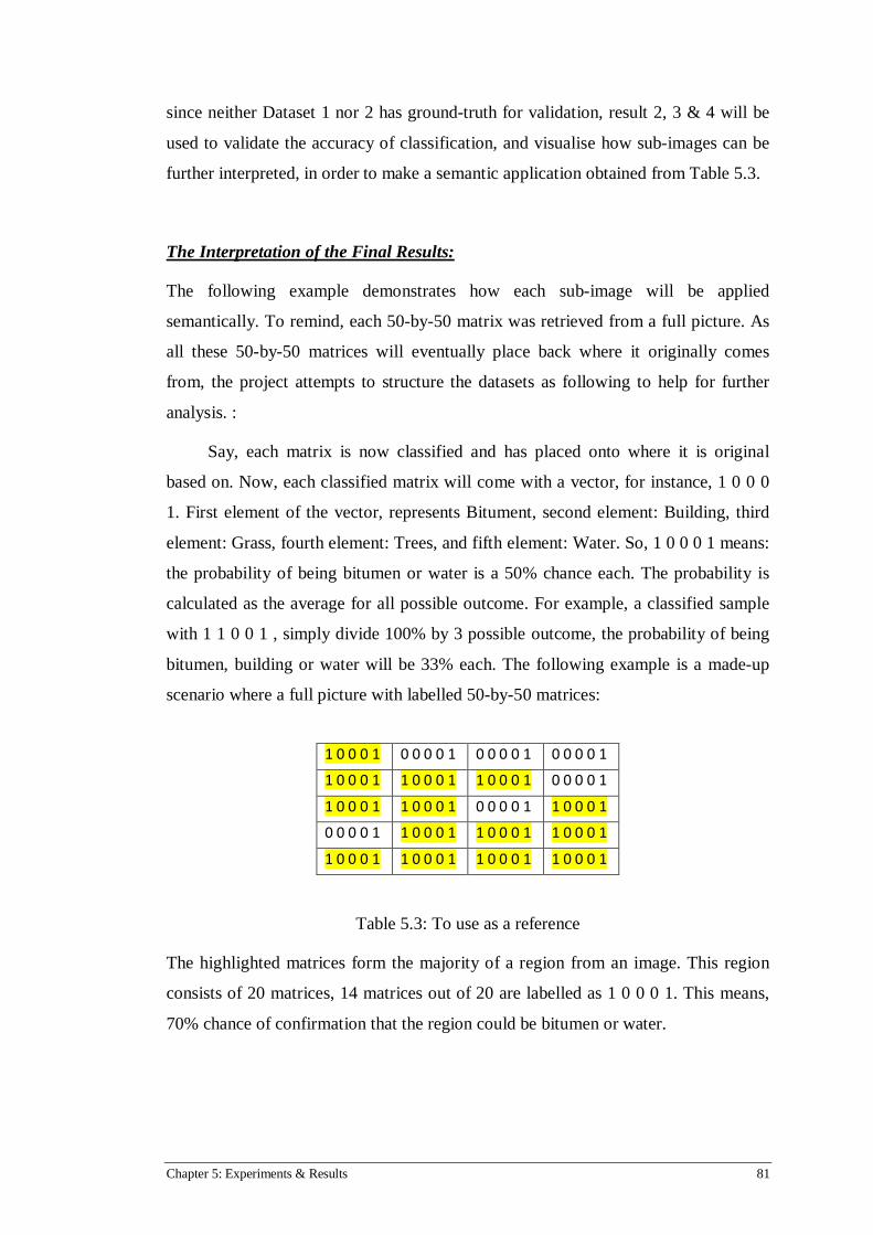
Chapter 5: Experiments & Results 81
since neither Dataset 1 nor 2 has ground-truth for validation, result 2, 3 & 4 will be
used to validate the accuracy of classification, and visualise how sub-images can be
further interpreted, in order to make a semantic application obtained from Table 5.3.
The Interpretation of the Final Results:
The following example demonstrates how each sub-image will be applied
semantically. To remind, each 50-by-50 matrix was retrieved from a full picture. As
all these 50-by-50 matrices will eventually place back where it originally comes
from, the project attempts to structure the datasets as following to help for further
analysis. :
Say, each matrix is now classified and has placed onto where it is original
based on. Now, each classified matrix will come with a vector, for instance, 1 0 0 0
1. First element of the vector, represents Bitument, second element: Building, third
element: Grass, fourth element: Trees, and fifth element: Water. So, 1 0 0 0 1 means:
the probability of being bitumen or water is a 50% chance each. The probability is
calculated as the average for all possible outcome. For example, a classified sample
with 1 1 0 0 1 , simply divide 100% by 3 possible outcome, the probability of being
bitumen, building or water will be 33% each. The following example is a made-up
scenario where a full picture with labelled 50-by-50 matrices:
1 0 0 0 1 0 0 0 0 1 0 0 0 0 1 0 0 0 0 1
1 0 0 0 1 1 0 0 0 1 1 0 0 0 1 0 0 0 0 1
1 0 0 0 1 1 0 0 0 1 0 0 0 0 1 1 0 0 0 1
0 0 0 0 1 1 0 0 0 1 1 0 0 0 1 1 0 0 0 1
1 0 0 0 1 1 0 0 0 1 1 0 0 0 1 1 0 0 0 1
Table 5.3: To use as a reference
The highlighted matrices form the majority of a region from an image. This region
consists of 20 matrices, 14 matrices out of 20 are labelled as 1 0 0 0 1. This means,
70% chance of confirmation that the region could be bitumen or water.

Chapter 5: Experiments & Results 82
Result 2 & Analysis:
Figure 5.6: A result produced by the LSTM algorithm which the input is organised
based on the xy Chromaticity Diagram.
indicates water indicates trees or water indicates trees or grass indicates bitumen or building indicates misclassification
The result of Figure 5.6 demonstrates the output which will be used for the UAV to
perform the final site selection. As described in the previous subsection, if the UAV
zoomed into the particular red-highlighted square box (shown on Figure 5.6), the
UAV has to further calculate the possible decision based on probabilities, in this
case, the result shows that 88.9% chance of confirmation that the region could be
water. This method also attempts to validate the accuracy of classification obtained
from Table 5.3 as there is no ground-truth support. Overall, result 1 produce 98.9%
of accuracy based on the contextual support. For instance, the sample in yellow-
highlighted is likely to be bitumen rather than grass as supported by the contextual
knowledge. Another reason for the high accuracy is due to a small sample size of
dataset. It is possible to increase performance as small samples do not influence by a

Chapter 5: Experiments & Results 83
more general case. Result 1 also show which sample is misclassified. This
misclassification is due to the ambiguity of the definition such as should the region
be considered as trees or bitumen. The misclassification can be also produced by the
“noise” within the datasets such as shadow.
Result 3 & Analysis:
Figure 5.7: An image produced by the LSTM algorithm and the input organised
based on the xy Chromaticity Diagram.
indicates bitumen or building indicates trees or grass indicates misclassification
Result 3 is another experiment demonstrates all sub-images results obtained from the
LSTM placed back to its original image. Result 3 misclassified 41 samples out of
300 samples based on the contextual information. Again, the misclassification is due
to the ambiguity of the definition as well as the “noise” within the datasets, also
depending on how the sample is divided. However, the way xy Chromaticity

Chapter 5: Experiments & Results 84
Diagram extracts information has assisted the LSTM technique classified 98.6%
correctly.
Result 4 & Analysis:
Figure 5.8: A result produced by the LSTM algorithm which the input is organised
based on the xy Chromaticity Diagram.
indicates trees or grass indicates undefinable object indicates misclassification
Result 4 shows 99.7% of the classifications are correctly assigned the labels. As the
picture of result 3 is a simple classification, the criteria of classification are tightened.
For instance, the contextual information is not used. Some samples are shared by the
class of trees or grass, and the class of undefinable object, in this case, the sample
will be stated as correctly classified subject to whether the class occupies more than
half of the sample. For instance, the sample in yellow-highlighted is considered as
the class of undefinable object, as the class has occupied the sample more than half
of the area.

Chapter 5: Experiments & Results 85
5.4 SUMMARY
This chapter aimed at conducting several experiments to validate the
applicability of LSTM approaches for image texture classification. Each of
them served a purpose; Experiment 1 shows the LSTM can also work well in
classifying the imaging datasets. In Experiment 2, for task 1 uses Feedforward
Neural Network to test the reliability of the datasets as well as aiming to
compare the results with the LSTM. Task 2 shows the use of xy Chromaticity
Diagram technique can also deliver a reliable result by recognising the pixels’
location, while this process does not require a complicated procedure.
Importantly, this technique reduces processing time largely in order to deal
with urgent situation such as, emergency landing in our case. Experiment 3
demonstrates how the findings of this project can contribute to the larger
project, which focuses on developing a structured process to land the UAVs
safely during emergency situation. Images were unknown to the algorithm and
results confirm the potential of LSTM for classifying image texture using aerial
imagery from an UAV.


Chapter 6: Conclusion & Future Work 87
Chapter 6: Conclusion & Future Work
The objective of this thesis is to identify a Machine Learning technique with
the potential of developing into end-to-end features engineering, as well as a multi-
usage Machine Learning technique, especially for imaging datasets. The Long Short
Term Memory architecture is found to be one of the most promising architectures as
it provides the two main features: the long term memory and the ability of forgetting,
which we perceive as important abilities in order to analyse datasets which is huge
and highly-correlated. As a result, the LSTM with its attributes alone could possibly
become a central machine which uses for analysing all kind of datasets. Although the
LSTM has not been using to analyse imaging datasets, if imaging datasets can be
structured into patterns, in fact, all Machine Learning techniques have the ability to
classify the datasets. The only consideration is that not all Machine Learning
techniques can perform a dynamic behaviour. In the meantime, many concerns are
discovered during the interpretation of the imaging datasets phrase such as cognitive
bias. In addition, it is necessary to understand briefly the sciences that form imaging
datasets, in order to structure a useful modelling as well as a stabilised datasets. To
achieve the goal of reducing big variation in the RGB values, the imaging data is
converted into another space, being able to successfully stabilise the fluctuation of
the RGB values by recognising the pixels’ locations based on the xy Chromaticity
Diagram. In addition, due to the stability of values in the xy Chromaticity colour
space, small sample sizes of datasets is sufficient to perform the texture
classification.
6.1 FUTURE WORK
The future work will be further divided into two areas: Machine Learning Technique
and Object Recognition.
6.1.1 Machine Learning Technique – Neural Network Architecture
The layer of Max-pooling:

Chapter 6: Conclusion & Future Work 88
The main idea of using NN is due to the architecture that allows mathematics
to act intelligently on datasets. For instance, the functionality of firing rate gives the
network an ability to bring the most relevant signal to next level for further analysis.
Some of the mathematics used in the NN may not give any flexibility such as max-
pooling. Max-pooling is a technique to pick the most significant number on a group
dropping out the rest. By dropping out the rest, it means the rest of the information is
no longer important. Indirectly, the technique throws out the ability of the entire
network to behave dynamically. Perhaps, the question is more about timing, when is
the right timing to apply the idea of max-pooling methodology. However, the current
layer of using max-pooling method acts as throwing the network’s ability to perform
a change in decision making.
Weight Guessing:
Although most of the time weight guessing can increase the efficiency of the
network, this approach does not provide a sense of standardization across different
types of datasets, especially the very first layer of neurons to accept the inputs.
Weight guessing means that the network randomly generates a weight to attach with
the inputs to perform weight searching across the entire network; while the concept
behind a biological neuron in terms of weight, it is affected by the external factors.
Although the mathematical modelling that describes the biological neuron is
oversimplified, the concept of how an actual neuron works does lend its idea to
develop a sophisticated computing architecture. For the long run, weight guessing is
essential to be standardised, so that the network has better framework to create its
standalone space.
In short, the concept and methods of using max-pooling and weight guessing
are the two main restrictions at this stage, limiting proceedings to the next level of
development. All assumptions are made according to the current research discovery
as well as within our knowledge.

Chapter 6: Conclusion & Future Work 89
6.1.2 Object Recognition
The physics theory may consider being useful at this stage.
One of the main discoveries from this project is that pixels are not yet a
statistical datasets. Statistical datasets means that the data is ready for statistical
approaches to extract describable information. The logic of the research findings tells
us that pixels are still considered physical datasets, which means that the information
carried by the datasets can meaningfully be extracted based on the physics theories or
concepts. This logic is built because all pixels present are the brightness and colour
information. The brightness information corresponds to how many photons are
reflected; while colour information subjects to which types (wavelength) of photons
are bounced off, both depend on the moment when the light strike on the object and,
the camera catches this process. The camera caught this process and stores the final
result on a template, which is the digital image in this case.
Fortunately, all the information is needed for the human perception is the
wavelength of red, green, and blue colour. However, this information that relates on
human perception is also fairly interesting to think that, all objects must reflect,
absorb or transmit the three wavelengths: red, green and blue. This is because by
relying on these three wavelengths, they nearly produce a full range of colours.
Indirectly, the phenomenon implies that these three wavelengths may have the most
distinct force to bring impact onto the electrons; while the rest of the wavelengths
can be triggered between these three forces (red, green, and blue). To some extent,
these three wavelengths must possess some kind of deep connections in order to play
the key role, which may help to process the imaging datasets.
Regardless of what colour we see, the key point is that the natural phenomenon
that describes the behaviour of the electron falls under a certain range of possibility.
Since the result of different colour emission largely depends on the transition
between electrons’ orbital levels, this natural phenomenon forms a condition that
tells us a range of likelihood. As there is only a certain range of likelihood, it is
possible to use the brightness and colouring templates (a digital image), as the final
reference to trace the likelihood of the colour emission. The idea is to use a digital
image as a clue or reference, to track the direction of the light and the properties of
the object, which indirectly gives the information on the relationship between
surrounding pixels, and this is when the relationship between pixels can be analysed.

Chapter 6: Conclusion & Future Work 90
The idea of using physics theory is just the beginning; this approach will be
complex as it requires many building blocks to conclude the relationships between
surrounding pixels or the regions. However, every processing stage does have a
pattern, and Machine Learning techniques can come in at the particular stage to seek
for the relationship. Overall, physics theory seems more appealing to deal with the
imaging datasets. However, the research in this area alone will spend a considerable
amount of time and effort to build a concrete foundation.
Matrix Theory may be used as geometric or shape comparison.
In the long run, the position of the pixel provides important information about
the attributes of objects such as, the height of a tree, the radius of a drinking cup, or
many other geometric or shape comparisons. When the process comes to this stage,
we see that the relationship between pixels becomes relevant. To keep the location
information of pixels corresponding to its position of an image, this can be done by
using the matrix theory.
However, statistical approaches are not functioning in this manner where it
gives the position of the pixels, but to summarise the representations that describe the
object. The techniques of summarising the representations are also informative and
doable, perhaps, the concern is more on the numbers of processing steps before the
datasets is ready for statistical use. If these steps are skipped, the next layer of
calculation will be either intense or struggling.
Furthermore, matrix theory can be seen to behave a standalone space, which
means that the operation of matrix does not care whatever information is stored in its
element, all its concern is the dimension of the matrix. Therefore, the basic concept
of the matrix is to perform some calculations between points from space A to space
B, where they must have a relationship. As long as there is a pattern, Machine
Learning techniques can be used to seek for relationship, but not as the main
approach which starts from the beginning of pre-processing phrase, all the way to the
end of making decision stage.
To put all information into conclusion, the project discovered during the
research that, perhaps, the Machine Learning techniques itself is still capable to

Chapter 6: Conclusion & Future Work 91
perform image analysis at this stage; instead, the problem is more coming from the
imaging datasets itself, which most of the time complicates the Machine Learning
techniques, in order to disentangle complex information within the datasets. As a
result, the physics and the matrix theory are suggested to simplify the information
carried by the digital images, provided the computer vision is the goal to achieve. In
the meantime, there are also many improvements need to be done within the neural
network architecture, especially the first layer when accepting the inputs and, the
concept that frames the functionality at each layer in the network. Therefore, a few
concerns such as the max-pooling and weight guessing are essential to be
standardised, before the network can form its own space to use across all kind of data
types. All these concerns together, we see that the use of peephole connection is
unimportant at this stage, but this idea of predicting ahead is definitely powerful in
the future.


Bibliography 93
Bibliography
Ahuja, N. (1982). Dot pattern processing using voronoi neighbourhoods. IEEE Transactzons on Pattern Analyszs and Machzne Intellzgence. Retrieved from http://vision.ai.illinois.edu/publications/dot_pattern_TPAMI_1982.pdf
Beck, J., Sutter, A., & Ivry, R. (1987). Spatial frequency channels and perceptual grouping in texture segregation. Computer Vision, Graphics and Image Processing, 37(2), p. 299–325.
Bengio, Y., Courville, A., & Vincent, P. (2013). Representation Learning: A Review and New Perspectives. IEEE Trans. PAMI, special issue Learning Deep Architectures. Retrieved from: http://www.iro.umontreal.ca/~lisa/pointeurs/TPAMISI-2012-04-0260-1.pdf
Bengio, Y., & LeCun, Yann. (2007). Scaling Learning Algorithms towards AI. Large-Scale Kernel Machines. Retrieved from http://yann.lecun.com/exdb/publis/pdf/bengio-lecun-07.pdf
Bishop, C. (1995). Neural Networks for Pattern Recognition. Oxford University Press, Inc., ISBN 0198538642.
Blake, S., & Jebara, T. (2009). Structure preserving embedding. Proceedings of the 26th Annual International Conference on Machine Learning. Retrieved from http://www.metablake.com/spe/spe-icml09.pdf
Bringsjord, S. (15 August 2006). Artificial Intelligence. Retrieved from http://kryten.mm.rpi.edu/SEP/index8.html
Broomhead, D., & Lowe, D. (1988). Multivariate functional interpolation and adaptive networks. Complex Systems, 2:321 – 355.
Caelli, T. & Moraglia, G. (1985). On the detection of gabor signals and discrimination of gabor textures. Vision Research, 25(5), p. 671–684.
Cauwerts, C. (n.d.). Colour Perception. Retrieved from https://www.educate-sustainability.eu/portal/content/colour-perception
Cimpoi, M., Maji, S., and Vedaldi, A. (2014). Deep convolutional filter banks for texture recognition and segmentation. CoRR, abs/1411.6836.
Ciresan, D. C., Meier, U., Gambardella, L. M., & Schmidhuber, J. (2010). Deep Big Simple Neural Nets For Handwritten Digit Recognition. Neural Computation 22(12): 3207-3220, 2010.
Ciresan, D. C., Meier, U., Masci, J., Gambardella, L. M., & Schmidhuber, J. (2012). Flexible, high performance convolutional neural networks for image classification. In IJCAI, pp. 1237–1242.
Ciresan, D. C., Meier, U., & Schmidhuber, J. (2012). Transfer Learning for Latin and Chinese Characters with Deep Neural Networks. Proc. IJCNN 2012, p 1301-1306, 2012.

Bibliography 94
Collobert, R. (2011). Deep Learning for Efficient Discriminative Parsing. Retrieved from http://ronan.collobert.com/pub/matos/2011_parsing_aistats.pdf
Davis, L. (1979). Shape matching using relaxation techniques. IEEE Trans. Pattern Anal. Mach. Intell. Vol. PAMI-1, p 86-88.
Daugman, J. G. (1985). Uncertainty relation for resolution in space, spatial frequency, and orientation optimized by two-dimensional visual cortical filters. Journal of the Optical Society of America, 2(3), p. 1160– 1169.
Dyer, C., Rosenfeld, A., & Samet, H. (1980). Region representation: boundary codes from Quadtree. Commumications of the ACM, p.171-179.
Deng, L., & Yu, D., (2014). Deep Learning: Methods and Applications. Foundations and Trends in Signal Processing [PDF version], ISBN 978-1-60198-814-0, p.197-387. doi: : 10.1561/2000000039
Fitzgerald, D., Walker, R., & Campell, D. (2005). A Vision Based Forced Landing Site Selection System for Autonomous UAV. Retrieved from http://eprints.qut.edu.au/2765/1/2765_1.pdf
Freitas, N. d. (2015). Deep Learning Lecture 12: Recurrent Neural Nets and LSTMs. Retrieved from https://www.youtube.com/watch?v=56TYLaQN4N8
Gallery Yopriceville, (18 July 2015). Oack Tree PNG Clipart Picture. Retrieved from http://gallery.yopriceville.com/Free-Clipart-Pictures/Trees-PNG-Clipart/Oack_Tree_PNG_Clipart_Picture#.Va-qVPmqqko
Gers, F. (2001) Long Short-Term Memory in Recurrent Neural Networks. Diplom in Physik, Universitat ¨ Hannover, Deutschland de nationalite´ allemande Retrieved from http://www.felixgers.de/papers/phd.pdf
Graves, A. (2007) Supervised Sequence Labelling with Recurrent Neural Networks. Retrieved from http://www.cs.toronto.edu/~graves/phd.pdf
Graves, A., Fernandez, S., Schmidhuber, J. (2007). Multi-Dimensional Recurrent Neural Networks.Intl. Conf. on Artificial Neural Networks ICANN'07.
Graves, A., Mohamed, A., & Hinton, G. E. (2013). Speech Recognition with Deep Recurrent Neural Networks. ICASSP 2013, Vancouver.
Greff, K., Srivastava, R. K., & Schmidhuber, J. (2015). Training Very Deep Networks. Advances in Neural Information Processing Systems (NIPS), in press.
Haralick, R., Shanmugam, K., & Dinstein, I. (1973) Textural Features for Image Classification. IEEE Trans. on Systems, Man and Cybernetics, SMC–3(6):610–621
Haralick, R., & Watson, L. (1981). A facet model for image data. CGIP, 15, p. 113-129.
Hastie, T., Tibshirani, R., & Friedman, J. (2009). The Elements of Statistical Learning [PDF version], ISBN 978-0-387-84857-7, p.348. doi: 10.1007/b94608

Bibliography 95
Herta, C. (2016) Reber Grammar. Retrieved from http://christianherta.de/lehre/dataScience/machineLearning/neuralNetworks/reberGrammar.php
Hong,T. H., Shneier, M., & Rosenfeld, A. (1982). Border extraction using linked edge pyramids. IEEE Transactions on Systems, Man and Cybernetics, 12(5), p. 660–668.
Hinton, G. E. (2007). Learning multiple layers of representation. Trends in Cognitive Sciences,11, p. 428-434. Retrieved from http://www.cs.toronto.edu/~fritz/absps/tics.pdf
Hochreiter, S. (1991). Untersuchungen zu dynamischen neuronalen Netzen. Diploma thesis, TU Munich.
Hochreiter, S., & Schmidhuber, J. (1997). Long Short-Term Memory. Neural Computation, 9(8):1735–1780
Hopfield, J. J. (April, 1982). Neural networks and physical systems with emergent collective computational abilities. PNAS, 79(8):2554-2558.
Klawonn, F., Berthold, M.R., & Ada, Iris. (2009). Data Mining. Retrieved from http://www.hs-kl.de/~amueller/vorlesungen/dtm/04d_klassenbildung.pdf
Kohonen, T. (1989). Self-organization and associative memory: 3rd edition.Springer-Verlag New York, Inc., New York, NY, USA. ISBN 0-387-51387-6
Kubo, S., & Kadla, J.F. (2003). The formation of strong intermolecular interactions in immiscible blends of poly(vinyl alcohol) (PVA) and lignin. Biomacromolecules, 4, 561.
Krizhevsky, A., Sutskever, I., & Hinton, G. (2012). Imagenet classification with deep convolutional neural networks. In Advances in Neural Information Processing Systems 25, pages 1106–1114.
Landscape Wallpaper. (2014). Retrieved from http://hdnatur.com/landscape-wallpaper-1920x1080-images-6-hd-wallpaper.html
Larochelle, H., Bengio, Y., Louradour, J., & Lamblin, P. (2009). Exploring strategies for training deep neural networks. Journal of Machine Learning Research, 10, 1–40.
Lee, G. (20 October 2014). Machine-Learning Maestro Michael Jordan on the Delusions of Big Data and Other Huge Engineering Efforts. IEEE Spectrum. Retrieved from http://spectrum.ieee.org/robotics/artificial-intelligence/machinelearning-maestro-michael-jordan-on-the-delusions-of-big-data-and-other-huge-engineering-efforts
Linnainmaa, S. (1970). The representation of the cumulative rounding error of an algorithm as a Taylor expansion of the local rounding errors. Master's Thesis (in Finnish), Univ. Helsinki.
Julesz, B. (1981). Textons, the elements of texture perception, and their interactions. Nature, 290, p. 91–97.

Bibliography 96
Julesz, B., & Bergen, J. R. (1983). Textons, the fundamental elements in preattentive vision and perception of textures. Bell Systems Technical Journal, 62(6), p. 1619–1645.
Ojala, T., Pietikainen, M., & Harwood, D. (1996) A comparative study of tecture measures with classification based on featured distribution. Pattern Recognition, 29(1):51-59.
Ojala, T., Valkealahti, K., Oja, E., & Pietikainen, M. (2001). Texture discrimination with muldimensional distributions of signed gray-level differences. Pattern Recognition,34 (2001), p. 727-739. Retrieved from http://www.mediateam.oulu.fi/publications/pdf/58.pdf
Malik, J., & Perona, P. (1990). Preattentive texture discrimination with early vision mechanism. Journal of the Optical Society of America, 7(5), p. 923–932.
Manik, V. (2004). Statistical Approaches To Texture Classification. Robotics Research Group Department of Engineering Science University of Oxford. Retrieved from http://research.microsoft.com/en-us/um/people/manik/pubs/varma04a.pdf
Marčelja, S. (1980). Mathematical description of the responses of simple cortical cells. Department of Applied Mathematics, Research School of Physical Sciences, Institute of Advanced Studies, The Australian National University, Canberra, A.CT. 2600, Australia. Retrieved from https://www.osapublishing.org/view_article.cfm?gotourl=https%3A%2F%2Fwww%2Eosapublishing%2Eorg%2FDirectPDFAccess%2F5870AA5B-9120-AD37-C39669CE9A1B17C0_57758%2Fjosa-70-11-1297%2Epdf%3Fda%3D1%26id%3D57758%26seq%3D0%26mobile%3Dno&org
Matheron, G. (1967) Eléments pour une théorie des milieux poreux. Paris: Masson.
Marr, D. (1982). Vision. Freeman, Chap 2, pp 54-78.
Mejias, L. (2014). Classifying natural aerial scenery for autonomous aircraft emergency landing. The 2014 International Conference on Unmanned Aerial Systems (ICUAS’14),1236-1242. Retrieved from http://eprints.qut.edu.au/72213/1/icuas_14.pdf
Mitchell, T. (1997). Machine Learning, McGraw Hill. ISBN 0-07-042807-7, p.2
Pentland, A. P. (1984). SHADING INTO TEXTURE. AAAI-84 Proceedings. Retrieved from http://aaaipress.org/Papers/AAAI/1984/AAAI84-063.pdf
Pieroni, G. G. (2013). Issues on Machine Vision. Springer.
Pigments. (18 July 2015). The Pennsylvania State University. Retrieved from https://online.science.psu.edu/biol011_sandbox_7239/node/7287
Pygas, M. (18 July 2015). 35 Insane Optical Illusions That Will Make You Question Your Sanity. Retrieved from http://hdnatur.com/landscape-wallpaper-1920x1080-images-6-hd-wallpaper.html

Bibliography 97
Ramsundar, B., Kearnes, S., Riley, P., Webster, D., Konerding, D., & Pande, V. (2015). Massively Multitask Networks for Drug Discovery. arXiv. Retrieved from http://arxiv.org/pdf/1502.02072.pdf
Robinson, A. J., & Fallside, F. (1987). The utility driven dynamic error propagation network. Technical Report CUED/F-INFENG/TR.1, Cambridge University Engineering Department.
Rosenblatt, F. (1958). The perceptron: A probabilistic model for information storage and organization in the brain. Psychological Review, 65:386 – 408.
Rumelhart, D. E., Hinton, G. E., & Williams, R. J. (1986). Learning internal representations by error propagation, p. 318 – 362. MIT Press, Cambridge, MA, USA, 1986. ISBN 0-262-68053-X
Schachter, B. J., Rosenfeld, A., & DAVIS, L. S. (1978). Random mosaic models for textures. IEEE Transactions on Systems, Man, and Cybernetics, 8, p. 694–702.
Scherer, S., Chamberlain, L. J., & Singh, S. (2012). Autonomous landing at unprepared sites by a full-scale helicopter. Robotics and Autonomous Systems, vol. 60, no. 12, pp. 1545–1562.
Schimidhuber, J. (1 Jan 2000). Long Short-Term Memory: Tutorial on LSTM Recurrent Networks. Retrieved from http://people.idsia.ch/~juergen/lstm/sld017.htm
Schmidhuber, J. (2014). Deep Learning in neural networks: An overview. Neural Network, 61(2015), 85-117. doi: 10.1016/j.neunet.2014.09.003
Schmidhuber, J. (18 July 2015). Recurrent Neural Networks. Retrieved from http://people.idsia.ch/~juergen/rnn.html
Serra J. (1982). Image Analysis and Mathematical Morphology. London: Academic Press.
Shen, Y.F., Rahman, Z., Krusienski, D., & Li, J. (2013). A vision-based automatic safe landing-site detection system. Aerospace and Electronic Systems, IEEE Transactions on, vol. 49, no. 1, pp. 294–311.
Siegelmann, H. T., & Sontag, E. D. (1991). Turing computability with neural nets. Applied Mathematics Letters, 4(6):77-80.
Simonyan, K., & Zisserman, A. (2014). Very deep convolutional networks for large-scale image recognition. CoRR, abs/1409.1556.
Singh, H. (28 April 2014). How Punjabi, the Gurnukhi Language and Grammar Systems. Retrieved from http://wingsforall.com/bhagouauty/blog/tag/be-happy-philselfology/
Stollenga, M., Byeon, W., Liwicki, M., & Schmidhuber, J. (2015). Parallel Multi-Dimensional LSTM, With Application to Fast Biomedical Volumetric Image Segmentation. Advances in Neural Information Processing Systems (NIPS), in press.

Bibliography 98
Talbot, D. (6 January 2015). Nvidia Demos a Car Computer Trained with “Deep Learning”. MIT Technology Review. Retrieved from http://www.technologyreview.com/news/533936/ces-2015-nvidia-demos-a-car-computer-trained-with-deep-learning/
Tomita, F., & Tsuji, S. (1990). Computer Analysis of Visual Textures. Kluwer Academic Publishers, Dordrecht, p. 13-36.
Tuceryan, M., & Jain, A. K. (1990). Testure segmentation using Voronoi polygons. IEEE Transactions on Pattern Analysis and Machine intelligence 12, 211 216.
Tuceryan, M., & Jain, A.K. (1993). Texture analysis. In: Chen, C.H., Pau, L.F. and Wang, P.S.P., Eds., Handbook of Pattern Recognition & Computer Vision, World Scientific Pub Co Inc., Singapore City. doi:10.1142/9789814343138_0010
Turner, M. R. (1986). Texture discrimination by gabor functions. Biological Cybernetics, 55, p. 71–82.
Unser, M. (1995). Texture classification and segmentation using wavelet frames. IEEE Trans. Image Process. 4 (11), 1549– 1560.
Voorhees, H., & Poggio, T. (1987). Detecting textons and texture boundaries in natural images. In: Proceedings of the First International Conference on Computer Vision. p. 250-258, 1987.
Wang, X., Yang, M., Zhu, S., & Lin, Y. (2013). Regionlets for generic object detection. In ICCV.
Werbos, P. J. (1988). Generalization of backpropagation with application to a recurrent gas market model. Neural Networks, 1.
Williams, R. J., & Zipser, D. (1995). Gradient-based learning algorithms for recurrent networks and their computational complexity. In Y. Chauvin and D. E. Rumelhart, editors, Back-propagation: Theory, Architectures and Applications, pages 433–486. Lawrence Erlbaum Publishers, Hillsdale, N.J. Retrieved from citeseer.nj.nec.com/williams95gradientbased. html.
Wu, Zhirong. (2015). Recurrent Neural Networks. Retrieved from http://vision.princeton.edu/courses/COS598/2015sp/slides/RNN/RNN.pdf
Xu, J. (1997). Bidirectional Recurrent Neural Networks. IEEE Trans. On Signal Processing. Retrieved from http://deeplearning.cs.cmu.edu/notes/BRNN_Felix_2013_09_25.pdf
Zucker, S. W. (1976). Region growing: Childhood and adolescence. Computer Graphics and Image Processing 5, p. 382-99.

Appendices 99
Appendices
Appendix A
The Steps of constructing Datasets
A 50-by-50 water sample with RGB Colour Space
An example of a 5-by-5 matrix retrieved from a 50-by-50 Water Class image.
89 89 90 89 88 90 90 90 89 88 91 91 90 88 87 92 91 89 88 87 92 90 88 87 87
82 82 82 81 81 82 82 82 81 80 82 82 81 80 80 83 82 80 79 80 82 81 79 79 80
59 60 61 59 58 60 60 60 59 58 61 60 59 58 58 60 59 58 57 58 60 59 58 57 58
Red Channel Green Channel Blue Channel Divide each channel by 255:
Red Channel Green Channel Blue Channel
A 5-by-5 matrix

Appendices 100
All channels must go through calculation below:
if ( eachImage <= D65) eachImage = eachImage / 12.92; else eachImage = ( ( eachImage + 0.055 ) / 1.055 ).^ 2.4; end
Below is the result of each channel:
Red Channel Green Channel Blue Channel
Now the data is ready to be transformed.
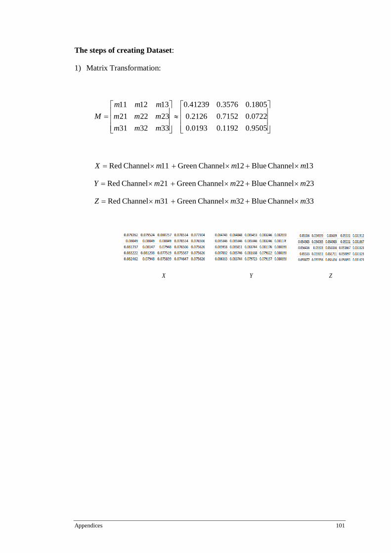
Appendices 101
The steps of creating Dataset:
1) Matrix Transformation:
≈
=
0.95050.11920.01930.07220.71520.21260.18050.35760.41239
333231232221131211
mmmmmmmmm
M
13Channel Blue 21ChannelGreen 11Channel Red mmmX ×+×+×=
23Channel Blue 22ChannelGreen 21Channel Red mmmY ×+×+×=
33Channel Blue 23ChannelGreen 31Channel Red mmmZ ×+×+×=
X Y Z

Appendices 102
2) xy Chromaticity Diagram:
a. )(
ofelement each ZYX
Xx++
=
b. )(
ofelement each ZYX
Yy++
=
coordinatex − coordinatey −
25th pixel falls into the grid of 29th in the sequence.

Appendices 103
3) Input Data is prepared as following steps:
a) xy Chromaticity Diagram is divided into grids based on the range its fall. i.e.:
x = 0 – 0.1; y = 0.1 – 0.2 => the 1st element of the sequence.
x = 0 – 0.1; y = 0.2 – 0.3 => the 2nd element of the sequence.
b) The total elements of a sequence are 45. The 1st element to 44th element
represents grids and the 45th element is the error catcher (ensuring
programming and computation are correct). In the 5-by-5 matrix above:
To total up the numbers of pixels of an image, fall into each grid: 0 0 0 0 0 0 0 0 0 0 0 0 0 0 0 0 0 0 0 0 0 0 0 0 0 0 0 0 25 0 0 0 0 0 0 0 0 0 0 0 0 0 0 0 0 To turn the grids with pixels into binary code – input data is now ready: 0 0 0 0 0 0 0 0 0 0 0 0 0 0 0 0 0 0 0 0 0 0 0 0 0 0 0 0 1 0 0 0 0 0 0 0 0 0 0 0 0 0 0 0 0
4) Target Input is organised as below:
BITUMEN 1 0 0 0 0
BUILDING 0 1 0 0 0
GRASS 0 0 1 0 0
TREES 0 0 0 1 0
WATER 0 0 0 0 1
Target Data is now ready.
5) Input Data combines Target Data:
In our case: 0 0 0 0 0 0 0 0 0 0 0 0 0 0 0 0 0 0 0 0 0 0 0 0 0 0 0 0 1 0 0 0 0 0 0 0 0 0 0 0 0 0 0 0 0 0 0 0 0 1
NOTED: each row represents a 50-by-50 image.
Appendices 104
Appendix B
The Confusion Matrices of 7 Images
The following are normalized Confusion Matrices of True Positive Rate and
False Negative Rate for each image.
Normalized Confusion Matrices Images
(1)
(2)
(3)
(4)

Appendices 105
(5)
(6)
(7)