a denotational semantics approach to functional and logic ... · frank steven kent silbermann. a...
TRANSCRIPT

A Denotational Semantics Approach to Functional and Logic Programming
TR89-030
August, 1989
Frank S.K. Silbermann
The University of North Carolina at Chapel Hill Department of Computer Science CB#3175, Sitterson Hall Chapel Hill, NC 27599-3175
UNC is an Equal OpportunityjAfflrmative Action Institution.

A Denotational Semantics Approach to Functional and Logic Programming
by
FrankS. K. Silbermann
A dissertation submitted to the faculty of the University of North Carolina at Chapel Hill in partial fulfillment of the requirements for the degree of Doctor of Philosophy in Computer Science.
Chapel Hill
1989

@1989
Frank S. K. Silbermann
ALL RIGHTS RESERVED
11

FRANK STEVEN KENT SILBERMANN. A Denotational Semantics Approach to
Functional and Logic Programming (Under the direction of Bharat Jayaraman.)
ABSTRACT
This dissertation addresses the problem of incorporating into lazy higher-order
functional programming the relational programming capability of Horn logic. The
language design is based on set abstraction, a feature whose denotational semantics
has until now not been rigorously defined. A novel approach is taken in constructing
an operational semantics directly from the denotational description.
The main results of this dissertation are:
(i) Relative set abstraction can combine lazy higher-order functional program
ming with not only first-order Horn logic, but also with a useful subset of higher
order Horn logic. Sets, as well as functions, can be treated as first-class objects.
(ii) Angelic powerdomains provide the semantic foundation for relative set ab
straction.
(iii) The computation rule appropriate for this language is a modified parallel
outermost, rather than the more familiar left-most rule.
(iv) Optimizations incorporating ideas from narrowing and resolution greatly
improve the efficiency of the interpreter, while maintaining correctness.
Ill

ACKNOWLEDGEMENTS
Bharat Jayaraman suggested I investigate unifying functional and logic pro
gramming via a lazy functional language with set abstraction. It was a fruitful
topic, drawing together a variety of programming language design ideas. He gave
his time, encouragement and patience generously.
I also thank my other committee members, David Plaisted, Dean Brock, Jan
Prins and Gyula Mago for their insightful and constructive comments on preliminary
drafts and oral presentations of preliminary work. David Plaisted and Dean Brock
were especially helpful in taking the time to read and comment under severe time
limitations. Don Stanat also provided many useful comments. Special thanks also
to David Schmidt of Kansas State University, who answered some difficult technical
questions.
This research was supported by grant DCR 8603609 from the National Science
Foundation and contract N 00014-86-K-0680 from the Office of Naval Research.
iv
TABLE OF CONTENTS
1 INTRODUCTION 1
1.1 Declarative vs. Imperative Languages 1
1.2 Paradigms of Declarative Programming 3
1.2.1 Functional Programming 3
1.2.2 (Horn) Logic Programming 4
1.2.3 Equational Logic Programming 7
1.2.4 Functional and Logic Programming Combinations 9
1.3 Proposed Approach 11
1.3.1 Relative Set Abstraction 12
1.3.2 Denotational Semantics 14
1.3.3 Correct Operational Semantics 15
1.3.4 Optimization 15
1.3.5 Scope of the Research 15
2 THE POWERFUL LANGUAGE 17
2.1 Syntax of Constructs 17
2.2 Program Examples 19
2.3 Translating Horn Logic to PowerFuL 21
2.3.1 Converting Horn Logic to Set Logic 21
2.3.2 Converting Set Logic to PowerFuL 22
2.3.3 Discussion 23
3 DENOTATIONAL SEMANTICS 25
3.1 Semantic Domains 25
3.2 Powerdomains 30
3.3 Denotational Semantics of PowerFuL 33
3.3.1 Semantic Equations 34
3.3.2 Coercions 38
3.4 Summary 39
v

4 FROM DENOTATIONAL TO OPERATIONAL SEMANTICS 41
4.1 Recursion and Least Fixpoints 43
4.2 Computation Rules and Safety 44
4.3 Computation of Primitives 4 7
4.4 Operational Semantics of PowerFuL 50
4.4.1 Termination of !3-Reduction 51
4.4.2 Desiderata for the Computation Rule 52
4.4.3 PowerFuL's Reduced Parallel-Outermost Rule 56
4.4.4 Example 59
4.6 Summary 60
5 POWERFUL SEMANTIC PRIMITIVES 62
5.1 Boolean Input Primitives 62
5.2 Atomic Input Primitives 63
5.3 List Primitives 64
5.4 The Powerdomain Primitive 64
5.5 Coercions 65
5.6 Run-time Typechecking 67
5. 7 Equality 69
5.8 Summary 71
6 OPTIMIZATIONS 72
6.1 Avoiding Generate-and-Test 72
6.2 Logical Variable Abstraction 74
6.3 Simplfying Primitives with Logical Variables 76
6.3.1 Technique 1: Simple Reduction 77
6.3.2 Technique 2: Splitting by Type 78
6.3.3 Technique 3: Splitting on Equality 79
6.3.4 Discussion 83
6.4 Example 84
6.5 Correctness Results 89
6.6 Summary 89
VI

7 CONCLUSIONS
7.1 Results and Contributions
7.2 Further Work
References
Vll
91
91
93
95
1 INTRODUCTION
This chapter places functional and Horn logic programming within the gen
eral context of declarative programming languages. After reviewing previous func
tional/relational combinations, we provide an overview of our approach.
1.1 Declarative vs. Imperative Languages
Programming languages can be divided into two broad categories: zmpera
tive languages, which includes languages such as Fortran, Pascal and Ada [M83],
and declarative languages, which includes (declarative subsets of) languages such
as Prolog [CM81] and Lisp [M65]. One way to appreciate their difference is via
Kowalski's celebrated equation "Algorithm = Logic + Control," [K79] meaning
that an algorithm may be described as a combination of logical relationships and
execution control. Imperative programming languages, having evolved from Von
Neumann machine languages, express the program control explicitly, and leave the
program logic implicit in the form of assertions that are invariant at various control
points. Declarative programming languages reverse the relative emphasis of logic
and control; they express the program logic explicitly, leaving much of the control
implicit. In contrast to the machine orientation of imperative languages, declarative
languages are programmer-oriented, and their syntax and semantics are based on
mathematical theories predating the electronic computer.
Two important declarative subgroups are functional and logic. The most
expressive functional programming languages (those which treat functions as com
putational objects) are based on lambda calculus; these include pure Scheme [AS85]
and pure ML [M84], Miranda [T85] and Haskell [HW88]. Simpler (first-order)
functional languages have been based on an algebra of programs [B78] and recur
sion equation systems [085]. Most logic programming languages have likewise been
based on the first-order predicate calculus [VK76, GM84], higher-order predicate
calculus [MN86], and also equational logic [085, YS86, F84].
The benefits of declarative languages are, firstly that algorithms expressed in a
declarative language are often easier to understand than when expressed in a more
procedural language, since the parts of a program combine in a more predictable
way. Often the declarative programs are shorter. Because of their absence of side
effects and explicit sequencing, they have great potential for parallel execution.
Even on purely sequential machines they execute efficiently enough to be useful
in many applications [P87]. As the ratio of programmer costs to hardware costs
rises, and with programs becoming longer and more complex, declarative languages
are becoming ever more attractive. Furthermore, declarative languages show great
potential for implementation on massively parallel hardware [CK81, D74, GJ89,
LWH88, MSO, M82]. Declarative languages do not over specify the order of op
erations, and for many subcalculations execution order may be chosen arbitrarily.
When execution order is known to be irrelevant, sub-calculations may be freely
executed in parallel.
Another advantage of declarative over imperative languages, and indeed, a cen
tral focus of this dissertation, is that the semantics of declarative languages can be
more easily given a mathematically rigorous treatment. Programming language
semantics is a study of the association between programs and the mathematical
objects which are their meaning. Different methods have been proposed to describe
this association, e.g., denotational, operational, axiomatic, etc. [P81]. To specify
the semantics of a language denotationally means to specify functions that assign
mathematical objects to the programs and to parts of the programs in such a way
that the semantics of a program expression depends only on the semantics (i.e. not
the form) of its subexpressions. This kind of semantics seems most useful for de
scribing the language constructs, i.e. for encapsulating the essence of the language
design. Since the constructs of a declarative language are patterned after mathemat
ical ideas, denotational semantics would seem seem to be the easiest way to describe
a declarative language. Operational semantics specifies an abstract machine which
would compute the output of a program. That is, an operational semantics can be
viewed as a high-level description of a possible implementation. Since the constructs
of an imperative language are designed with conventional hardware capabilities in
mind, operational semantics would seem to be the easiest way to describe an im-
2

perative language. Axiomatic semantics seems most useful for proving properties
of specific programs in a language. Since we are interested in language design and
implementation, we will concentrate on denotational and operational semantics. As,
we are designing a declarative language, the defining semantics is the denotational;
the operational semantics will be considered correct only to the extent it agrees
with the denotational.
1.2 Paradigms of Declarative Programming
Various declarative paradigms have evolved independently of each other. We
discuss some of the more popular ones, emphasizing their unique features.
1.2.1 Functional Programming
· The functional programming paradigm, based on function definition and appli
cation, offers powerful tools for program modularization and abstraction. Typically,
a computation may be decomposed into a hierarchy of smaller components. For in
stance, one operation might produce a data structure used by the next. In a purely
imperative style, rather than defining each operation independently, references to
their common data structures make the definitions of these operations mutually
dependent. This makes it difficult to understand one part of the program inde
pendently of the rest, and hinders the reuse of code. In a more functional style of
programming, an operation can provide data for the next via function composition.
For instance, an expression denoting the result of one function is used as an input
argument to another. The location or name of the intermediary result need not be
explicitly given, thus allowing the two functions to be defined independently of each
other. More specific features common to functional programming are listed below.
1) With a form of outermost, or lazy evaluation, the data structure defined by
an argument expression is computed only to the extent necessary for its caller. With
this strategy, a function can define a data structure that is conceptually infinite,
such as an infinite list. With infinite lists, even interactive input-output can be
described in a purely functional notation, as shown by Henderson [HSOb]. The
functions being composed can be modeled as concurrent processes.
2) Functional languages permit higher-order objects, i.e., functions may take
other functions as arguments and produce other functions as results. With this
feature, one can more easily abstract code common to several routines. With the
3

ability to create general-purpose program fragments, more program parts can be
easily reused in new systems.
3) Static Jcoping permits functions to be defined within the context of other
function definitions. This provides modularization via hierarchical functional de
composition and supports information hiding.
4) To help the programmer avoid errors, many programming languages provide
a type system. An object's type constrains the range of values it may take, so that
gross errors are caught early. Many functional programming languages provide
polymorphic typing, so that typing can be parameterized.
5) To enhance its acceptance for practical programming, powerful compilation
techniques have been developed, such as incremental compilation and combinator
approaches [P87].
To give a flavor of the functional style of programming, we present a small
program, which given a function to insert a binary operator between components
of a list, easily defines functions to sum lists of numbers, compute their products,
and even to append lists:
reduce (func, identity, list) is if null(l) then identity else func( head(list), reduce( func, identity, tail(list)) )
sumlist is lambda(list). reduce(+, 0, list)
prodlist is lambda(list). reduce( *• 1, list)
append(a, b) is reduce( cons, b, a)
1.2.2 (Horn) Logic Programming
In logic programming, computations are specified via logical constraints. In
stead of defining the solution as a function from input to output, one merely states,
in the form of relationJ, the properties the solution must satisfy. This gives pro
grams a more flexible execution moding; not until execution need it be d~termined
which parameters of a relation will be given values and which parameters are to be
computed. Execution is a search procedure to find one or more solutions. In this
sense, logic programming can be even more declarative than functional programs.
Its chief advantages are:
4
1) conceptual simplicity, in that a program can be viewed as a set of assertions
in first-order predicate logic; and
2) automatic availability of a function's inverse, i.e. when a function is pro
grammed as a relation between its input and its output, its inverse is also automat
ically defined.
The most popular form of logic programming is based on first-order Hom logic,
a subset of predicate logic. A Horn logic program defines and reasons with relations.
Conceptually speaking, each program clause states that for all instantiations of its
variables by first-order terms, if all the righthand side predicates are true, then so
is the predicate on the lefthand side. We use the term subgoal to refer to one of
the righthand side predicates. If a clause has no subgoals, then, for all possible
instantiations, the lefthand side predicate is true. Such a clause is called a unit
clause.
For instance, one can describe the appendfunction as a relation between its
input arguments and its output, as in the following Horn logic program:
append( [], X, X). append( [HIT], Y, [HIZ]) :-append( T, Y, Z).
The goal is to find a set of bindings for the variables so that all the predicates in the
user query are true. In a user query, one can either provide two lists to be appended,
or one can request that two lists be found which, when appended, produce a known
list:
?- append( [1,2], [3,4], Ans).
?- append( left, Right, [1,2,3,4]).
Since the universe of first-order terms can be enumerated, one could, in princi
ple, generate all possible instantiations for the goal, and check each instantiation for
suitability by verifying, if possible, the truth of each instantiated goal predicate via a
derivation. A more efficient operational procedure, called resolution, tries to derive
the truth of the original uninstantiated user query, binding values to the variables
in the goal and program clauses only to the extent needed to keep the derivation
going. Such variables are called logical variables, in current Prolog terminology.
Two basic operations of the resolution procedure are unification and search. In
unification, the logical variables in a program and in the goal are given values so that
5

a predicate in the user query will equal the lefthand side predicate of the partially
instantiated program clause. When this can be done, the instantiated righthand
side of the program clause replaces the matched predicate in the user query. In first
order Horn logic, two terms are equal if and only if they are identical, so unification
can be efficiently implemented. Higher-order unification is much more difficult; in
fact, testing the equality of two higher-order terms is not decidable, in general [R86].
"Search" refers to the fact that, an any stage in the derivation, one may have
several applicable program clauses to choose from. Breadth-first search, in which
one tries all possible choices, will find all solutions. This property is called complete
ness. Usually however, a depth-first search implemented via backtracking is used,
because of its smaller space requirements. Depth-first search, however, sacrifices
completeness.
One disadvantage of first-order Horn logic programming is its lack of higher
order capability, i.e. the inability to use relations themselves as objects. Warren
described a way to encode some higher-order Horn logic programs within first
order Prolog [W83a]. The programmer associates a special (first-order) term with
each predicate to be passed as an argument (or returned as a result) in place of
the predicate itself. To apply the 'predicate', one calls a special 'apply' predicate,
which has recorded which predicates are associated with which terms, applying the
associated predicate. Though Warren has described a useful Prolog programming
technique, higher-order predicates defined via his technique may lack referential
transparency. Referential transparency requires that when two predicates name
the same relation, they may be interchanged anywhere in the program without
changing the program's declarative meaning (though execution efficiency may be
affected). With Warren's scheme, a "higher-order" predicate testing two input
predicates for equality would test the associated terms, instead. The term.encodings
might differ even if the predicates themselves define the same relation. Though
Warren's technique provides the desired linguistic expressiveness, the possibility of
nontransparent usage makes reasoning about programs more difficult. It is for this
same reason that we consider first-order logic insufficient as the basis for higher
order programming, in contrast to the position taken in [G88]. One would prefer
that higher-order capability be directly supported in the language's actual formal
semantics.
6
Seeing the limitations of Warren's encodings, researchers (MN86, R86] are in
vestigating programming languages based on subsets of of higher-order Horn logic.
Unfortunately, full higher-order predicate logic is uncomputable, so most approaches
restrict the higher-order capability to handle only specific subclasses of higher-order
objects, or impose restrictions limiting their use. Miller and Nadathur have de
scribed a form of Horn logic incorporating terms from Church's typed lambda cal
culus (MN86], introducing some higher-order capability. However, their functions
(lambda expressions) cannot be recursively defined and were not intended to pro
vide full higher-order capability. Rather, they intended their system to be a useful
tool for meta-programming, i.e. for building program transformation systems and
theorem provers.
The next section discusses another variation of logic programming based on
equational logic.
1.2.3 Equational Logic Programming
Though this dissertation does not deal explicitly with equational programming,
we feel that some discussion is warranted, as equational programming is capable of
combining many of the features of both functional and Horn logic programming
[085, F84, YS86, DP85]. Like Horn logic programming, certain forms of equational
programming compute by solving constraints (YS86, F84, DP85]. As in functional
programming, certain forms of equational programming can define functions, exe
cuting them with reasonable efficiency (085]. As with Hom logic programming, it
provides no higher-order capability.
In equational logic, rather than defining general predicates or relations, the
program is a collection of parameterized equalities between terms, each implying
that, for all instantiations of the (logical) variables, the two resulting terms are
equal. Alternatively, the equality of a parameterization can be made conditional
upon other pairs of terms being proven equal first. The goal of an equational logic
program is to instantiate a user query so as to make it a logical consequence of the
program.
To test whether two terms are equal, one uses the equations as substitutions,
to see whether one can rewrite the two terms to identical forms. This can be very
difficult, as one must compare each equivalent form of the left term in the goal
7
with each equivalent form of the right. Furthermore, for each term, the class of
equivalent terms may be infinite.
To avoid the computational problems of unrestricted equational programming,
term-rewriting systems were developed. In proving equality of two terms, the pro
gram equations are used in one dires:tion only, i.e. one instantiates a program
equation so that its left side matches a portion of the term being rewritten, and
that portion is then replaced by the instantiated right-hand side. In order to guar
antee the sufficiency of this mechanism, the equation set must be confluent. That
is, it must be guaranteed that, if a term can be rewritten using more than one equa
tion, all results must eventually converge to a common result. It is easiest to prove
confluence when it can be shown that rewriting is always guaranteed to terminate,
in which case, every term has a unique normal form, i.e., rewrites to a single term
which can no longer be rewritten.
Confluent and terminating term-rewriting systems are called canonical. When
a canonical term-rewriting system is viewed as an equational program, it has the
property that all equal terms will rewrite to a common term, called a normal form,
which cannot be further rewritten. This greatly increases the efficiency of the
equality test, as one need not only compare two normal forms to test whether
two terms are equal. However, one disadvantage of using canonical term-rewriting
systems for functional programming is that the termination requirement rules out
functions and relations operating on infinite data structures.
An operational mechanism known as narrowing (HSOa], which combines reduc
tion and unification, allows one to solve for logical variables (DP85] [YS86] in a
goal equation. This technique reduces the parameterized equation via the rewrite
rules as much as possible. When the presence of logical variables in the goal pre
vents further reduction, the variables are replaced by somewhat more defined values
(terms which may contain new logical variables) in order that reduction may con
tinue. When the equality becomes apparent, the accumulated bindings for the
logical variables provide the solution. For completeness, each time a logical vari
able is narrowed, one must compute in a breadth-first manner many alternative
narrowings. Unfortunately, the branching on narrowing tends to quickly get out of
hand.
Constructor-based equational programming systems (R85] (JS86] [F84b] seem
8

to ameliorate the above problems. Certain functors are taken as irreducible data
constructors, and other functors are assumed to name functions. An equation's left
side is restricted to contain only one function name, placed at the outermost level,
thus distinguishing between equations to define functions, and equations stating
properties of functions, and permitting only the former. A term now no longer
stands for itself, but rather denotes the no"rmal form (which is built solely of con
structors). With this restriction, the distinction between term-rewriting and first
order functional programming begins to blur, and with narrowing, one gains Horn
logic's capability to satisfy constraints, as seen in the following example:
append( [ ] , y) = y append([h I t], y) = cons(h, append(t, y))
?-append([1,2], [5,6]).
?-append(x, y) = [1, 2, 3].
In a constructor-based system, narrowing becomes more efficient (at each step, fewer
narrowings need be considered) [F84b] [JS86J. Where reduction without narrow
ing suffices, non-terminating programs (denoting infinite objects) might possibly be
supported. Proofs of confluence are still required, though they are perhaps easier to
find. In some ways, reduction, the operational strategy of functional programming,
resembles term-rewriting. We should therefore not be surprised if the operational
procedure of a language combining functional and logic programming would simi
larly resemble narrowing.
1.2.4 Functional and Logic Programming Combinations
Sometimes we wish to combine both functions and relations within one pro
gram. A number of attempts have been made to combine features of functional and
logic programming into a single language (see [BL86] for a recent survey). Either
one can add functional programming to a Horn logic base, or one can add relational
capability to a functional programming language.
Some have proposed adding function definition capability to Horn logic via
an equational theory [K83] [GM84]. The equational theory may be provided via a
canonical term rewriting system. Syntactic examination of a predicate's arguments
no longer suffices when judging whether a program clause is relevant. Instead, the
interpreter must ascertain whether a predicate's arguments might rewrite to terms
9
matching the program clause, or whether patterns in the program clause may be
rewritten to match the arguments. The computational complexity of this inference
mechanism is a major difficulty.
In describing his language Fresh [SP85], Smolka begins with a functional lan
guage, written in an equational style to incorporate pattern-matching, and describes
an operational semantics reminiscent of narrowing. The resulting language is very
expressive, providing a higher-order capability via a technique similar to Warren's
(described above). As with Warren's encodings, referential transparency is lost. It
is unclear what would be a meaningful purely declarative subset, as Smolka did not
provide a denotational description.
Though Horn logic relations are defined in predicate logic, these relations could
just as easily be described via set theory. In fact, Horn logic's model-theoretic and
fixed-point semantics are described in the language of set theory. One approach to
combining functional and logic programming is to add sets as another data type.
Robinson and Darlington were the first advocates of adding logic programming
capability to functional programming through set abstraction. In describing SU
PERLOGLISP [BRS82], Robinson suggests that a functional language should have
a construct denoting the complete set of solutions to a Horn logic program, and that
the user be able to build functions accepting such sets as arguments. Darlington
calls his extension absolute set abstraction [D83, DFP86] to distinguish it from rel
ative set abstraction, discussed later. Absolute set abstraction permits expressions
such as
{x: p(x)},
to denote define the set of all x satisfying p( x). In this approach, nondeterminism
is replaced by set union, and unification is performed to solve equations between
non-ground objects.
Robinson's language, SUPERLOGLISP, combines LISP and Horn logic through
absolute set abstraction. He develops many useful implementation ideas, but does
not develop a mathematical justification or a formal semantics. Since the base
language is LISP, LOGLISP has some higher-order capability, though its use is
restricted when accessing the relational features. As in LISP, stream-based pro
gramming is not supported, as arguments must be evaluated before being passed
10

to functions.
Darlington's approach is similar; however, his base functional language is lazy,
with polymorphic typing. In his recent paper [DFP86), Darlington sketched a par
tial and informal operational semantics. In [DG89), he described absolute set ab
straction in a strictly first-order equational language as a variation of narrowing in
term-rewriting systems.
The work of Darlington and Robinson leaves several important open problems:
In what way does this construct interact with other traditional functional language
features, such as infinite and higher-order objects? How can the presence of this
feature be reflected in the language's denotational semantics? Will all denotable sets
be computable? To our knowledge, these semantic issues have never been rigorously
worked out.
1.3 Proposed Approach
Our goal is a language incorporating both functional and logic programming,
and providing the following features:
1) Simple semantics through referential transparency. For instance, functions
should be completely described by the mapping defined; two alternative defini
tions describing the same mapping should be indistinguishable within the language.
Analogously, sets should be completely described by the elements contained; we
should not be able to distinguish two different expressions of the same set, though
orderings of the elements may differ. In other words, we would like to satisfy the
axiom of extensionality [877) for functions and sets.
2) Higher-order objects should be first-class, i.e., they can be used freely as
function or predicate arguments and results.
3) Possibility of efficient execution. Backtracking should not be used where
simple rewriting is sufficient, and the interpreter should not rely on computationally
explosive primitives, such as higher-order unification or unification relative to an
equational theory.
4) Verifiably correct execution mechanism, 1.e., the operational and denota
tional semantics should describe the same language.
We make functional programming with set abstraction the basis for our unified
11
declarative language because:
1) simple propagation of objects can be managed without equality tests (im
portant for higher-order objects);
2) it should be easier to add the constructs from as small and simple a language
as Horn logic into the larger and more complicated functional programming, rather
than vice-versa. Functional programming languages have a richer domain of objects,
compared with Horn logic's fiat domain, and therefore a larger variety of constructs;
and
3) ordinary functional computations not making use of set abstraction might
be executed without backtracking.
For simplicity, we will not consider typing mechanisms, whether polymorphic or
otherwise, though we see no reason why such a feature could not be added.
1.3.1 Relative Set Abstraction
Neither Robinson nor Darlington have been able to implement absolute set
abstraction as a first-class object, interacting freely with other functional language
features. Both Darlington and Robinson claim that implementation of absolute set
abstractions as first-class objects would require higher-order unification, which is
not always computable. Even so, some higher-order programs in their languages
would merely be unexecutable program specifications. Robinson has criticized exist
ing combinations of higher-order functional programming with first-order relational
programming as inelegant [R86]. His goal is to create a purely declarative func
tional language permitting higher-order relational programming, without arbitrary
unorthogonal restrictions on its features. But, this line of work has yet to be fully
explored.
Replacing absolute set abstraction with the semantically simpler relative set
abstraction, the notation avoids the suggestion that full higher-order logic program
ming capability ought to be available. This removes the sense of inelegance Robinson
noted. A typical relative set abstraction would be an expression of the form:
{f(x) : x E G and C(x)}.
Here, the generating set G is provided explicitly, and those elements x which satisfy
the condition C are used in computing elements of the new set. Compare this to
12

the form of a typical absolute set abstraction:
{f(x) : C(x)}.
Here, one "solves" the condition C for suitable values of x, each solution used to
compute an element f(x) of the denoted set.
The absolute construct is powerful, but its higher-order extension is problem
atic. The implementations of the languages of Darlington and Robinson restrict a
logical variable to represent only first-order terms. This restricted domain is anal
ogous to the Herbrand univer3e in first-order Horn logic. Thus weakened, absolute
set abstraction is no longer more powerful than relative set abstraction. This set
of first-order terms, T, can easily be expressed via a recursively-defined relative set
abstraction. Thus, any first-order absolute set abstraction can easily be expressed
as a relative set abstraction. For instance, the example above would be written as:
{f(x) : x E T and C(x)}.
We observe that relative set abstraction can al3o provide the needed logic pro
gramming capability. We prefer relative set abstraction because it has a more
tractable higher-order generalization. Not only is relative set abstraction as expres
sive as first-order absolute set abstraction (as shown above), but it can mix freely
with higher-order constructs, without requiring arbitrary first-order restrictions.
David Turner pioneered the use of relative set abstraction in a functional pro
gramming language, KRC [T81]. However, in his language, sets are implemented
as lists, and may be accessed as such, thus providing an implicit ordering on the
elements. This violates the semantics of sets and does not ensure fairness. If com
putation with one element of a generator set diverges, the next element is never
tried. With this kind of implementation, the construct is no longer described as
set abstraction; rather, one speaks of li3t comprehen3ion3 [P87]. We, in contrast,
advocate true relative set abstraction.
In our system, the set of first-order terms is provided as a (semantically un
necessary but operationally convenient) primitive. In computing a relative set ab
straction, only if a variable x is recognized as being enumerated from the set of
first-order terms is it treated as a logical variable. This special treatment is merely
an optimization to the default 'generate and test' mechanism. We show that these
set abstractions generated from the Herbrand universe can be identified, and opti-
13
mized to provide efficiency comparable to Darlington's procedure.
Thus, we propose a lazy, statically-scoped, higher-order functional language
with relative set abstraction, to combine higher-order functional and logic pro
gramming.
1.3.2 Denotational Semantics
A formal mathematical description of objects computed in this language, ob
jects such as atoms, lists, functions and sets, is given by the specification of the
semantic domain. The denotational semantics consists of this and a function map
ping of the language's syntactic statements to elements of the semantic domain.
We choose to define the language through denotational semantics because, through
this method, properties of a language can be determined at a glance. Consider for
example the denotational equation for a cons structure:
£[cons(expr1, expr2)] p = <(£[expr1] p), (£[expr2] p)>.
This equation describes the meaning of the expression, cons ( expr 1 , expr2),
in the .environment p, as depending upon the meaning of the sub expressions expr 1
and expr2. Note that the environment for one subexpression is unaffected by the
presence of the other subexpression. That is, the computation of expr1 can have
no side-effects that might influence the value of expr2. Therefore, the two subex
pressions can be computed independently, perhaps even in parallel. Through such
semantic equations the declarative nature of the language may be seen.
Though others have proposed languages combining functional and logic pro
gramming through set abstraction [BRS82J [DFP86], to our knowledge we are the
first to give a denotational description. One difficulty was finding a suitable domain
to represent set-valued objects. We have found that angelic powerdomains suffice,
and our reasons for this choice will be explained later in Chapter 3. Powerdomain
theory is usually used to describe nondeterministic languages, i.e. where a pro
gram is said to denote the set of objects which might be computed in any single
execution. Indeed, powerdomains were conceived for that very purpose. Our use
of powerdomain theory is unusual, in that, rather than describing the results of a
control structure (nondeterminism), it describes sets as an explicit data type.
14

1.3.3 Correct Operational Semantics
To demonstrate that the language is executable, we provide an operational se
mantics, and we show its correctness with respect to the denotational semantics.
To do so, we show that the denotational description's function to map syntactic
statements to the semantic domain can be viewed as a functional program for the
interpreter, written in terms of lambda expressions and primitive semantic func
tions. Each primitive function is defined via a set of equations, and implemented
through the use of these equations as simplification rules. This leaves unspecified
only the order of evaluation. We choose a variation of the parallel-outermost rule,
optimized in that some outermost computations may be delayed. That some de
gree of parallel evaluation is needed for complete evaluation of sets should not be
surprising; as a complete implementation of Hom-logic also requires a degree of
breadth-first evaluation.
1.3.4 Optimizations
The operational semantics described above is inefficient for two reasons. First,
it is pure interpretation; no provision has been made for compile-time pre-computation.
In defining the scope of this research, we chose to avoid such issues. Second, the op
erational semantics is inefficient when the set of first-order terms is the generator of
a relative set abstraction (analogous to an absolute set abstraction); the procedure
described above would blindly enumerate the infinite set of terms, instantiating a
copy of the abstraction for every possible term. To avoid this second cause of inef
ficiency, optimizations are provided which permit the enumerated variable in such
cases to be treated as a logical variable, instantiated only as needed to continue the
computation. This optimized operational semantics was inspired by the narrowing
technique from term rewriting systems [R85] and the resolution technique from logic
programming [184]. This development expresses our point of view that the logical
variable concept is best understood as an operational optimization, and not as part
of the language's declarative description.
1.3.5 Scope of the Research
This dissertation describes a programming language combining functional and
logic programming, and exhibiting the characteristics we have set forth as desirable.
The denotational semantics provides a deep understanding of the meaning of the
15

language constructs, and serves as a standard for correct implementation. We also
develop two variations of operational semantics. The first serves two purposes:
1) to demonstrate that the language can in fact be correctly implemented; and
2) to serve as a basis for the second operational semantics.
The second operational semantics contains optimizations essential for efficient logic
programming (the relation between the two operational semantics may be thought
of as analogous to that between Horn logic proof theory and the resolution method
[VK76]), and justifies our view that the logical variable is an operational, not a
declarative concept. In this dissertation, we do not discuss the detailed imple
mentation issues necessary for constructing a practical piece of software. Neither
operational semantics, if implemented directly, would be very fast. Rather, op
erational issues are considered only in so far as they give us a deeper theoretical
understanding of the language.
This introduction has given an overview of the dissertation, and a summary
of related work. The remaining chapters are as follows. Chapter 2 provides the
syntax of the new language, along with sample programs. Chapter 3 describes the
denotational semantics. Chapter 4 derives a simple operational semantics. Chapter
5 provides a detailed description of the semantic primitives. Chapter 6 improves
the operational semantics with optimizations for more efficient logic programming.
Chapter 7 discusses and summarizes the results of this research.
16
2 THE POWERFUL LANGUAGE
This chapter introduces a functional language with relative set abstraction. We
call the language PowerFuL, because Powerdomains provide the semantic basis
for the kind of set abstraction needed to unite Functional and Logic programming.
We first describe the syntactic features via BNF and informal explanation, and then
provide sample programs chosen to illustrate the constructs, and to show that any
first-order Horn logic program can be translated into PowerFuL.
Wishing to concentrate of semantic foundations, we emphasize the essential
features, leaving out many convenient syntactic niceties. For instance, we do not
provide the boolean connectives, as these can be easily programmed via the condi
tional. We also do not discuss (polymorphic) strong typing and numeric operations,
though these features are not incompatible with PowerFuL.
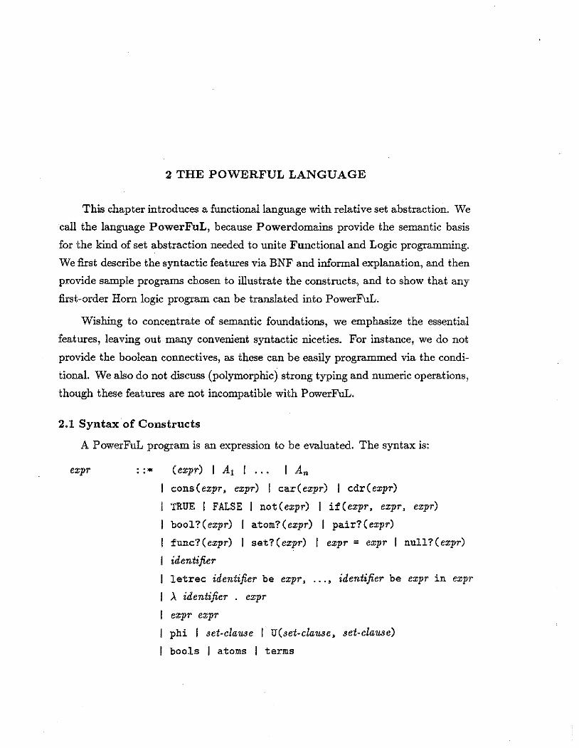
2.1 Syntax of Constructs
A PowerFuL program is an expression to be evaluated. The syntax is:
expr 0 0 = (expr) I A1 I .. . I An
cons(expr, expr) I car(expr) I cdr(expr)
TRUE I FALSE I not(expr) I if(expr, expr, expr)
bool?(expr)
func?(expr)
identifier
atom?(expr) I pair?(expr)
set? ( expr) I expr = expr I null? ( expr)
letrec identifier be expr, ... , identifier be expr in expr
>. identifier . expr
expr expr
phi I set-clause I U(set-clause, set-clause)
bools I atoms I terms
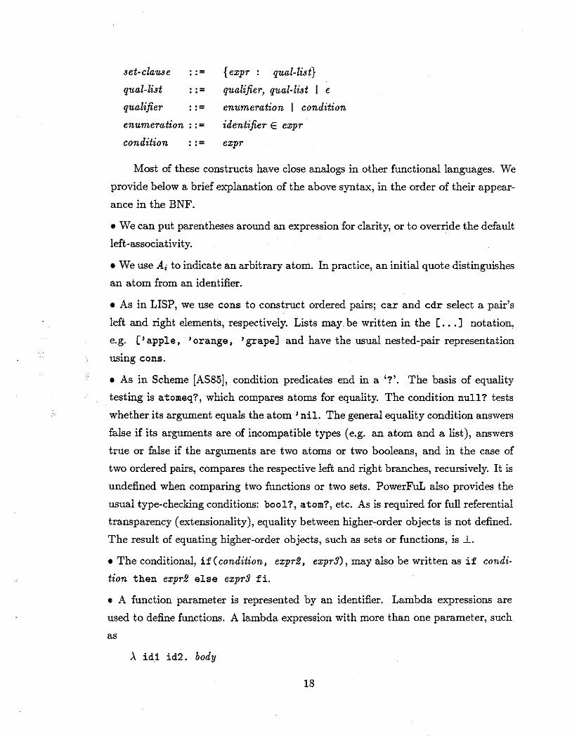
set-clause . ·= qual-list · · =
qualifier : : =
enumeration : : =
condition : : =
{ expr : qual-list}
qualifier, qual-list I e
enumeration I condition
identifier E expr
expr
Most of these constructs have close analogs in other functional languages. We
provide below a brief explanation of the above syntax, in the order of their appear
ance in the BNF.
• We can put parentheses around an expression for clarity, or to override the default
left-associativity.
• We use A; to indicate an arbitrary atom. In practice, an initial quote distinguishes
an atom from an identifier.
• As in LISP, we use cons to construct ordered pairs; car and cdr select a pair's
left and right elements, respectively. Lists may. be written in the [ ... ] notation,
e.g. ['apple, 'orange, 'grape] and have the usual nested-pair representation
usmg cons.
• As in Scheme [AS85], condition predicates end in a '?'. The basis of equality
testing is atomeq?, which compares atoms for equality. The condition null? tests
whether its argument equals the atom 'nil. The general equality condition answers
false if its arguments are of incompatible types (e.g. an atom and a list), answers
true or false if the arguments are two atoms or two booleans, and in the case of
two ordered pairs, compares the respective left and right branches, recursively. It is
undefined when comparing two functions or two sets. PowerFuL also provides the
usual type-checking conditions: bool?, atom?, etc. As is required for full referential
transparency (extensionality), equality between higher-order objects is not defined.
The result of equating higher-order objects, such as sets or functions, is l..
• The conditional, if (condition, expr2, expr:J), may also be written as if condi
tion then expr2 else expr:J fi.
• A function parameter is represented by an identifier. Lambda expressions are
used to define functions. A lambda expression with more than one parameter, such
as
,\ id1 id2. body
18
is syntactic sugar for a lambda expression with a single parameter x representing
a sequence. In this example, an occurrence of id2 in the body would be replaced
by cdr(x). Similarly, when applying a "multi-argument" lamba expression, the
argument list is converted to the appropriate list via cons.
• The syntactic form letrec is used to define statically scoped identifiers. A set of
identifiers may be defined via mutually recursive definitions. A program is invalid
if it contains a reference to an undefined identifier.
• Enumerations are the syntactic basis for relative set abstraction. Each identifier
introduced within the set-clause is associated with a set expression to provide possi
ble values. The scope of the enumerated identifier contains the principal expression
(left of the ': '), and also all qualifiers to the right of its introduction. In case of name
conflict, an identifier takes its value from the latest definition (innermost scope). In
any case, the scope of an enumerated identifier never reaches beyond the set-clause
of its introduction. When the qualifier is a condition, the expression to the left of
the ':' is in the denoted set only if the condition evaluates to true. When there
are no qualifiers to satisfy, the set-clause indicates a singleton set, and the ' : ' is
usually omitted. Expressions of the form U(set1 , ••• , se4,) are syntactic sugar
for a nesting of binary unions.
• The syntax bools refers to the set { TRUE, FALSE}. Similarly, atoms is the set
containing all the atoms A;. The set terms is a union of atoms, bools, and any
finite object which can be constructed by "cons" -ing together elements of those two
sets.
2.2 Program Examples
To illustrate the language constructs and to show their applicability for func
tional and logic programming, we now provide a series of short programs in Power
FuL.
19
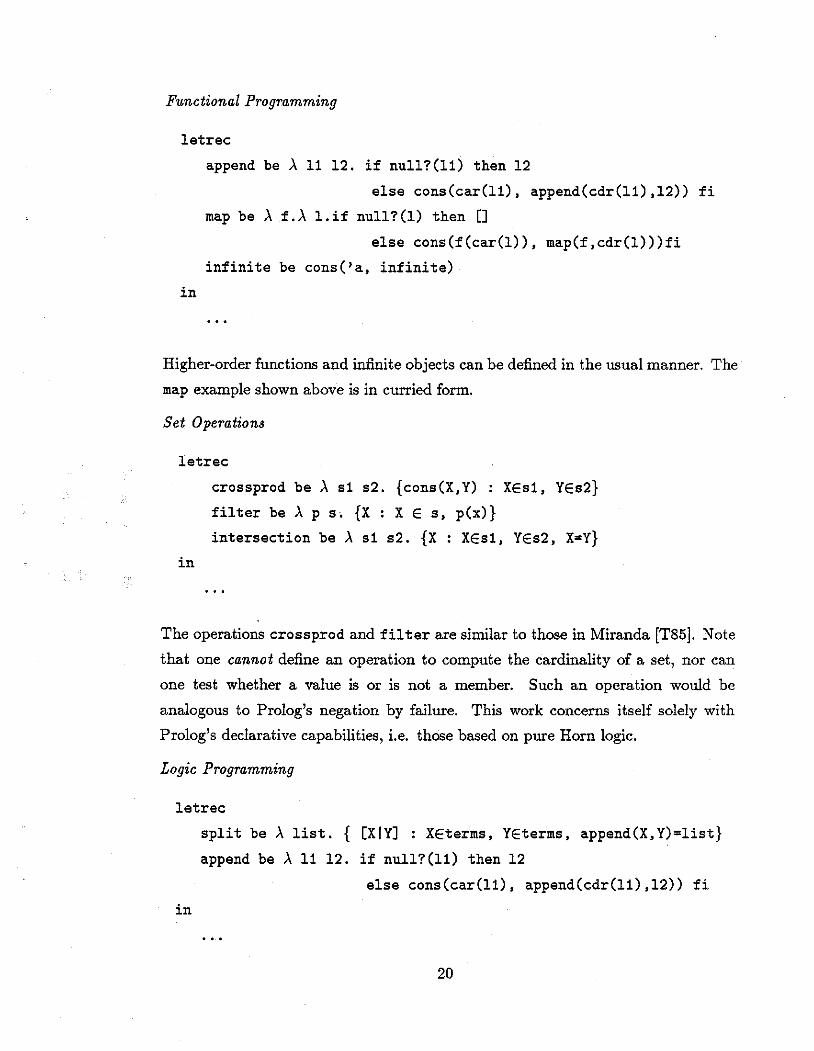
Functional Programming
letrec
in
append be A 11 12. if null?(l1) then 12
else cons(car(l1), append(cdr(l1),12)) fi
map be A f.A l.if null?(l) then []
else cons(f(car(l)), map(f,cdr(l)))fi
infinite be cons('a, infinite)
Higher-order functions and infinite objects can be defined in the usual manner. The
map example shown above is in curried form.
Set Operations
letrec
in
crossprod be A s1 s2. {cons(X,Y) : XEs1, YEs2}
filter be A p s. {X : X E s, p(x)}
intersection be A s1 s2. {X : XEs1, YEs2, X=Y}
The operations crossprod and filter are similar to those in Miranda [T85]. Note
that one cannot define an operation to compute the cardinality of a set, nor can
one test whether a value is or is not a member. Such an operation would be
analogous to Prolog's negation by failure. This work concerns itself solely with
Prolog's declarative capabilities, i.e. those based on pure Horn logic.
Logic Programming
letrec
split be A list. { [XIY] : XEterms, YEterms, append(X,Y)=list}
append be A 11 12. if null?(l1) then 12
else cons(car(l1), append(cdr(l1),12)) fi
in
20
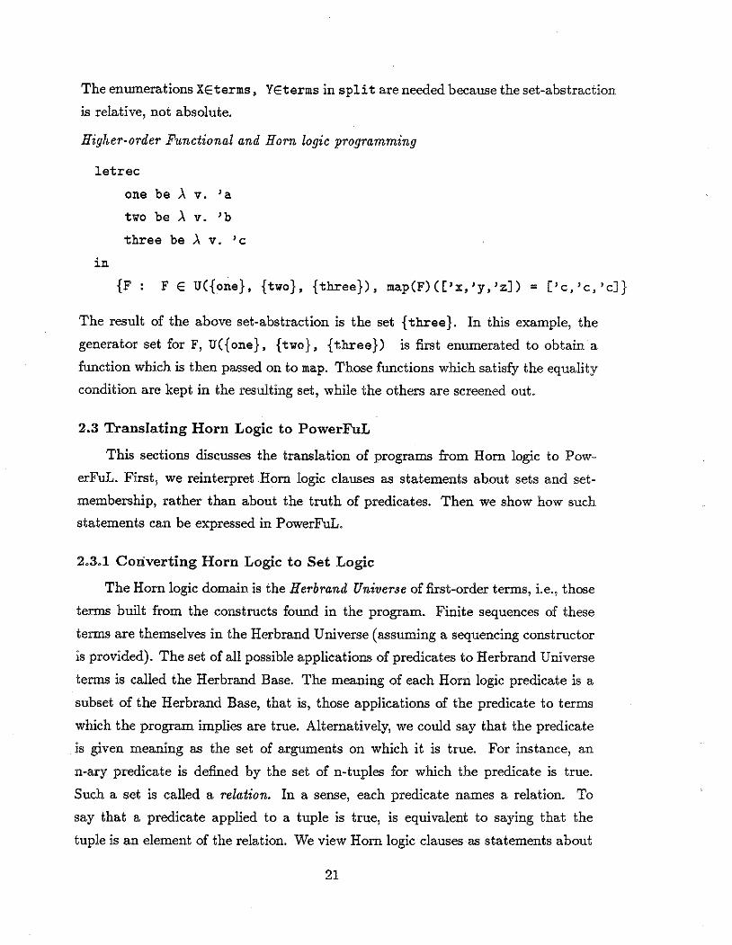
The enumerations XEterms, YEterms in split are needed because the set-abstraction
is relative, not absolute.
Higher-order Functional and Horn logic programming
letrec
in
one be ,\ v. ' a
two be ,\ v. 'b
three be ,\ v. 'c
{F: FE U({one}, {two}, {three}), map(F)(['x,'y,'z]) = ['c,'c,'c]}
The result of the above set-abstraction is the set {three}. In this example, the
generator set for F, U( {one}. {two}. {three}) is first enumerated to obtain a
function which is then passed on to map. Those functions which satisfy the equality
condition are kept in the resulting set, while the others are screened out.
2.3 Translating Horn Logic to PowerFuL
This sections discusses the translation of programs from Horn logic to Pow
erFuL. First, we reinterpret Horn logic clauses as statements about sets and set
membership, rather than about the truth of predicates. Then we show how such
statements can be expressed in PowerFuL.
2.3.1 Converting Horn Logic to Set Logic
The Horn logic domain is the Herbrand Universe of first-order terms, i.e., those
terms built from the constructs found in the program. Finite sequences of these
terms are themselves in the Herbrand Universe (assuming a sequencing constructor
is provided). The set of all possible applications of predicates to Herbrand Universe
terms is called the Herbrand Base. The meaning of each Horn logic predicate is a
subset of the Herbrand Base, that is, those applications of the predicate to terms
which the program implies are true. Alternatively, we could say that the predicate
is given meaning as the set of arguments on which it is true. For instance, an
n-ary predicate is defined by the set of n-tuples for which the predicate is true.
Such a set is called a relation. In a sense, each predicate names a relation. To
say that a predicate applied to a tuple is true, is equivalent to saying that the
tuple is an element of the relation. We view Horn logic clauses as statements about
21

set membership, where each set is a relation representing a predicate. Where a
conventional Prolog program asserts P(tuple ), we could equivalently assert that
tuple E P, where P now refers to a set.
For example, consider the following program and goal, written in Prolog syntax
[CM81].
app ( [], Y, Y) .
app([HIT], Y, [HIZ]) ·- app(T, Y, Z).
rev ( [] , [] ) .
rev([HIT], Z) ·- rev(T, Y), app(Y, [H], Z).
?- rev(L, [a, b, c]).
With a syntax more oriented towards sets, we could write:
[ [] , Y, Y] E app
[ [HIT], Y, [HIZ] ] E app ·- [T, Y, Z] E app
[ [] , [] ] E rev
[ [HIT] , Y] E rev ·- [T, Z] E rev, [Z, [H] , Y] E app
?- [X, [a, b, c] ] E rev
Here, we have used mutually-recursive definite clauses to define sets (instead of
predicates). We could call this paradigm set logic programming, but it is really just
another syntax for Horn logic.
2.3.2 Converting Set Logic to PowerFuL
Any such first order definite-clause set-logic program can be routinely converted
into PowerFuL. The letrec command provides mutually recursive definitions, and
each clause will correspond to a relative set abstraction. Where a predicate/set was
defined with several clauses, we use a union of relative set abstractions. Within
a relative set abstraction, each logical variable must be formally introduced as
representing an element the Herbrand Universe, i.e. terms. To indicate that a
particular first-order term is a member of a particular set, one lets the set instantiate
an enumeration variable, and then one states that the enumeration variable equals
the specified term.
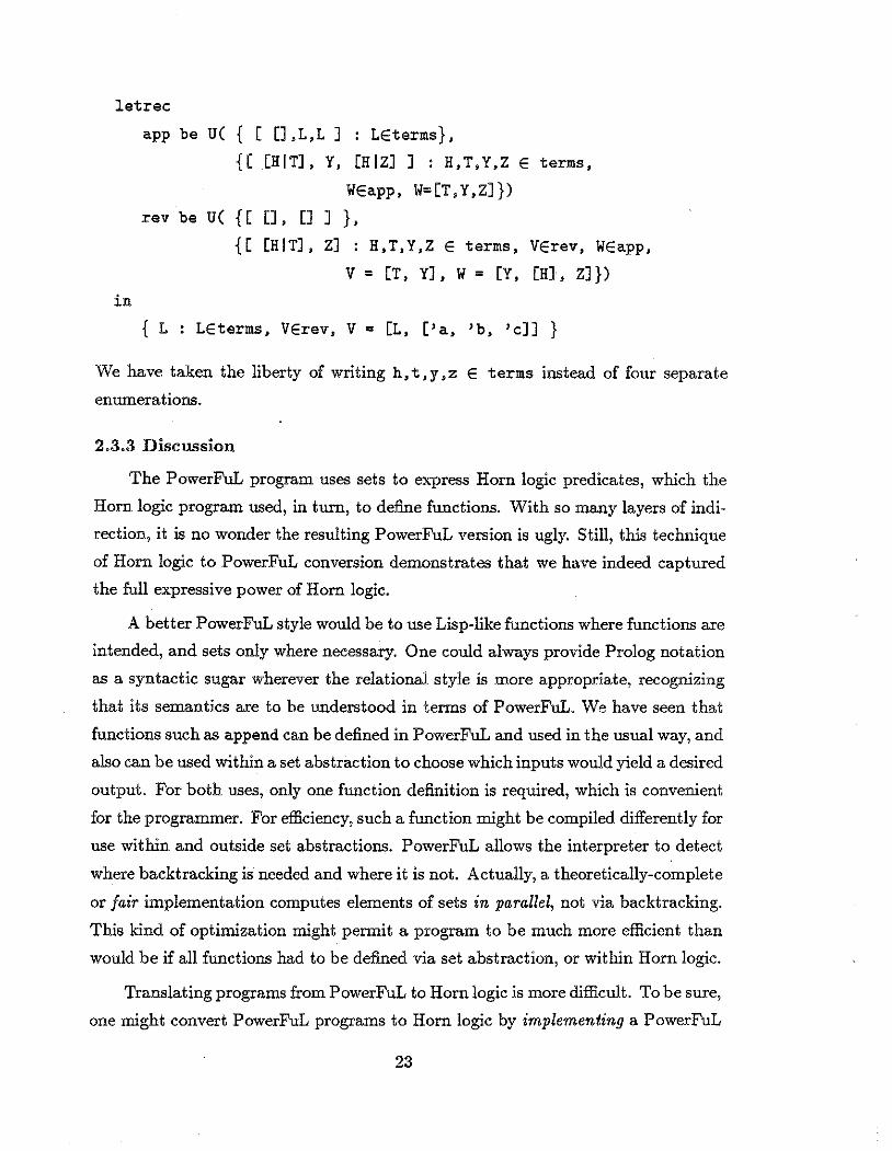
Converting the above program to PowerFuL syntax results in:
22
letrec
in
app be U( { [ [],L,L] : LEterms},
{[ [HIT], Y, [HI Z] ] : H, T, Y, Z E terms,
WEapp, W=[T,Y,Z]})
rev be U( {[ [], [] ] },
{[ [HIT], Z] : H,T,Y,Z E terms, VErev, WEapp,
V = [T, Y] , W = [Y, [H], ZJ})
{ L : LEterms, VErev, V = [L, ['a, 'b, 'c]] }
We have taken the liberty of writing h,t,y,z E terms instead of four separate
enumerations.
2.3.3 Discussion
The PowerFuL program uses sets to express Horn logic predicates, which the
Horn logic program used, in turn, to define functions. With so many layers of indi
rection, it is no wonder the resulting PowerFuL version is ugly. Still, this technique
of Horn logic to PowerFuL conversion demonstrates that we have indeed captured
the full expressive power of Horn logic.
A better PowerFuL style would be to use Lisp-like functions where functions are
intended, and sets only where necessary. One could always provide Prolog notation
as a syntactic sugar wherever the relational style is more appropriate, recognizing
that its semantics are to be understood in terms of PowerFuL. We have seen that
functions such as append can be defined in PowerFuL and used in the usual way, and
also can be used within a set abstraction to choose which inputs would yield a desired
output. For both uses, only one function definition is required, which is convenient
for the programmer. For efficiency, such a function might be compiled differently for
use within and outside set abstractions. PowerFuL allows the interpreter to detect
where backtracking is needed and where it is not. Actually, a theoretically-complete
or fair implementation computes elements of sets in parallel, not via backtracking.
This kind of optimization might permit a program to be much more efficient than
would be if all functions had to be defined via set abstraction, or within Horn logic.
Translating programs from PowerFuL to Horn logic is more difficult. To be sure,
one might convert PowerFuL programs to Horn logic by implementing a PowerFuL
23
interpreter in Horn logic, mapping PowerFuL's higher-order domain into Horn logic's
first-order domain. Since PowerFuL's semantic domain is much richer than that of
Horn logic, we see no general way to directly convert PowerFuL programs to Horn
logic. It is easier to restrict oneself to using only PowerFuL's first-order terms, than
to arbitrarily expand Horn logic's domain to include higher-order objects.
24
3 DENOTATIONAL SEMANTICS
This chapter presents a denotational definition of PowerFuL. After motivat
ing some fundamental terminology, we describe PowerFuL's semantic domain, and
define the function mapping PowerFuL syntax onto this domain. Especially note
worthy is the use of powerdomains as a semantic basis for a language with set
abstraction.
3.1 Semantic Domains
This section reviews some concepts and terminology from the Scott-Strachey
theory of denotational semantics. We will not try to provide a rigorous presentation,
but only try to motivate some of the basic definitions, which we have taken from
[S86J. A more detailed presentation can be found there, as well as in [S77]. Special
attention is given to the theory of powerdomains, a type of domain construction not
usually needed for functional programming.
Intuitively, a domain is the set of mathematical entities being manipulated as
data objects by a program. Actually, a domain is a partially ordered set with certain
technical properties which we will later define. Functions are defined recursively,
and it is conceivable that in defining a function, the program might not provide a
mapping for every possible input. So as to deal with true functions, rather than
partial functions, a domain will include a special element to mean undefined. This
element is usually written as l. (pronounced "bottom"). The undefined element
results when an undefined operation is requested (such as dividing by zero), or
when a definition is circular, possibly resulting in an infinite recursion.
Sometimes we wish to create new domains built upon domains already defined.
For instance, given domains D1 and D2 , we can create the domain D 1 X D2, which
consists of all ordered pairs of elements from domains D 1 and D 2 , respectively.
For instance, domain IJ_ x IJ_ contains all possible ordered pairs of elements from

l.J. .. The elements in this domain are defined to varying degrees. The least defined
element, .ll.L xl.L is the ordered pair where neither element defined, i.e. < .l, .l >. Note that, when combining domains like this, it is sometimes ambiguous as to
which domain's least element .l refers. Where necessary to avoid ambiguity, we will
subscript .l by the name of the domain intended. Here, the least defined element,
< .l, .l >, is less defined than < 2, .l >, which is, in turn less defined than
< 2, 3 >.
Definition 3.1: A binary relation !; over D x D is a. partial order if C is reflexive,
antisymmetric and transitive.
The partial ordering of ordered pairs depends upon the partial ordering on the
respective elements, as follows.
Definition 3.2: For ·any two elements < a1, b1 > and < a2, b2 > of D1 x D2,
< a1, b1 > !::::: < a2, b2 > iff both a1 !:::::n, a2 and b1 !:::::n2 b2.
Definition 3.3: For any partial ordering!; on a set D, if there exists an element
c E D such that for all d E D, c !; d, then c is the least element in D and is denoted
by the symbol .l.
Intuitively, one element A is less defined than or approximates another element
B if A can be created by replacing part of B with something undefined.
A list of elements for which each element approximates the next, (e.g. <
.l, .l >, < 1, .l >, < 1, 2 >) is called a chain.
Definition 3.4: For a partially ordered set D, a subset X of D is a chain iff X is
nonempty and for all a, b E X, either a!; b orb!; a.
The integer domain described above is very simple in that, aside from .lJ, all
its elements are fully defined. That is, for any A, B E I.L, A C B iff either A = .l1
or A= B. The longest possible chain is of length 2. A domain with this structure
is called a discrete or fiat domain. Another example of a discrete domain is the
domain of atoms (unlike the domain of integers, this domain has a finite number of
elements).
When the information content of two partially-defined elements is consistent,
there should exist an element which combines the information of each. We call such
an element an upper bound. This motivates the following definition.
26
Definition 3.5: For a set D with a partial ordering !;, the expression aU b denotes
the element in D (if it exists) such that:
1) a !; aU band b !; aU b; and
2) for all dE D, a C d and b!; dimply aU b !; d.
Definition 3.6: For a set D partially ordered by C and a subset X (sometimes
written as {x; I i E .i\f}) of D, UX (pronounced the least upper bound of X, and
sometimes written as U; x;) denotes the element of D (if it exists) such that:
1) for all x EX, x!; UX; and
2) for all dE D, if for all x; EX then x; C d, then U X !; d.
It is not always possible to automatically detect (e.g. in an interpreter) that
an arbitrary expression denotes .L When l. results from an infinite recursion,
evaluation will fail to terminate. While waiting for a result, we can never be sure
whether or not a result will eventually be forthcoming. Therefore, it is reasonable to
demand that, the less defined an argument to a function is (i.e. the more places l.
can be found), the less defined will be the output. This is expressed by a requirement
that functions be monotonic, as defined below.
Definition 3. 7: A function f : A ,_.. B is monotonic iff, for every (l, b E A, if
a !; b (using the the partial order of domain A), then f( a) !; f( b) (using the the
partial order of domain B).
A function may be either strict or non-strict. Informally, a function is strict if
the output is undefined whenever the input is undefined.
Definition 3.8: A function f: A>-+ B is strict iff, f(l.A) = l.s.
A constant function might be non-strict, for example the function f : h ~---> h which maps all inputs, including 1., to 1.
In higher-order functional programming, functions are themselves used as data
objects. So, domain D 1 >-+ D2 represents the domain of functions mapping elements
of domain D 1 to elements of domain D 2 • The partial order on functions is as follows.
Definition 3.9: Given two functions j, g : D 1 ,_. D 2 , we say that f !; g iff for all
dE Dll f(d)!; g(d).
If the input domain of a function has infinite size, then the domain of functions
will.contain chains of arbitrary length, perhaps even chains of infinite length. The
27
least function is defined as follows.
Definition 3.10: For any domains A and B, the least defined function Q is the
function f such that for all a E A, f(a) =.lB.
In a functional language, a function is typically defined as the least fizpoint of
a functional. These terms are defined below.
Definition 3.11: For domains A and B, a monotonic function f : A ~--+ B is
continuous iff for any chain X~ A, f(UX) = U{f(x) I x EX}. A function of
more than one variable is continuous iff it is continuous in each variable, individually.
Theorem 3.1: A monotonic function over a domain in which all chains are of finite
length (e.g. a discrete domain) is continuous.
Proof: Let A be a domain in which all chains are finite, and let f : A ~--+ B be
any monotonic function. Let X~ A be any (finite) chain in A. Because X is finite,
there must exist one element of the chain Xn such that for any x; E X, x; !;;;;; Xn and
therefore U; x; = Xn· Since f is monotonic, the set Y = {f(x;) I x; E X} is a finite
chaininBwithUY = f(xn)· Therefore,/(U;x;) = f(xn) = UY = U;J(x;).
End ofProof
Definition 3.12: A functional is a function r: D ~--+ D (usually D is a domain of
the form A>--> B).
Definition 3.13: For a functional T : D >--> D, dis a fizpoint of r iff dE D and
r(d)=d.
Definition 3.14: For a functional r: D >--> D, dis the least fizpoint (lfp) of riff d
is a fixpoint of r, and for any other fixpoint e of r, d !;;;;; e.
Theorem 3.2 (proved in [886]): If the domain D is a pointed cpo, then the least
fixpoint of a continuous functional r : D >--> D exists and is defined to be
lfp r = U{ri(.ln) I i 2: 0}, where Ti = ToTo ... or, i times.
Definition 3.15: The meaning of a recursive specification f = F(f) is taken to be
lfp(F), the least fixpoint of the functional denoted by F.
Consider the recursive definition, below, of the factorial function.
28
fact(x) = if((x=O),l,xxfact(x-1)).
The factorial is the least fixpoint of the functional
>.f. ,\x. if((x = O),l,x x f(x -1)).
In essence, the recursive definition defines a chain of non-recursive lambda
expressions, each of which we will call fact; for some integer i, each element of the
sequence expanding fact's recursion one step deeper than the previous, and thus
defining the factorial for yet another integer. This series of nonrecursive lambda
expressions forms a chain in h >--> I1., with the full factorial function being the
least upper bound of this chain. In general, when an infinite object, such as the
factorial function, is the least upper bound of a chain of elements in a domain, we
would like the least upper bound itself also to be in the domain. That is, we want
each domain to be a complete partial order. Since each domain will have a least
element, each domain will be a pointed cpo.
Definition 3.16: A partially ordered set D is a complete partial ordering ( cpo) iff
every chain in D has a least upper bound in D.
Definition 3.17: A complete partial ordering is a pointed complete partial ordering
(pointed cpo) iff it has a least element.
Applied to an argument x, the factorial function is computed by expanding
the recursion one step at a time. Mathematically, what we do is compute the chain
fact;( x ), until for some i the chain converges. The rationale for doing this will be
explained below.
Theorem 3.3: Any functional defined by the composition of monotonic functions
and the variable of the functional, is continuous.
The details of the proof of Theorem 3.3 use induction on the structure of the func
tional. It may be found in [M74].
Domain constructors must also be continuous, if we are to construct new do
mains from non-trivial base domains. For instance, in constructing the domain
(IJ. >-> I1.) X I1., we must be certain that < U; fact;, 2 > = U; < fact;, 2 >. The requirement that domain constructors be continuous plays an important role in
defining powerdomains, as seen in the next section. In defining PowerFuL's domain,
we only use domain constructors known to be continuous.
29

Another domain constructor is the sum. Given domains Dt, ... , Dn, the do
main (D1 + ... + Dn)J.. is a domain containing all the elements from then domains,
and a new least element .lv, + ... + Dn. For any d, e E (D1 + ... + Dn), d ~ e iff
either d = .lv, + ... + D. or both d and e came from the same component domain
D;, and d ~D; e.
Richer domains can sometimes be described as solutions to recursive domain
equations [S86]. For instance, the equation
D =(A + D x D)J..
describes the domain consisting of atoms, and nested ordered pairs whose leaves
are atoms, and are nested to arbitrary (and even infinite) depth. The equation is
actually read to say that domain D consists of the atoms plus the domain of ordered
pairs, the elements of these pairs coming from a domain isomorphic to D.
3.2 Powerdomains
The denotational semantics of set abstraction requires enriching the domain
with a new kind of object representing a set of simpler objects. Intuitively, given
a domain D, each element of domain D's powerdomain 'P(D) is to be viewed as a
set of elements from D. Powerdomain theory was originally developed to describe
the behavior of nondeterministic calculations, for which a program denotes a set of
possible results. The original application was operating system modelling, where
results depend on the random timing of events, as well as on the values of the inputs.
In describing powerdomains, we shall use examples in nondeterminism as motivation
for the theory. Be aware, however, that in PowerFuL we use powerdomains to
explicitly define sets within a deterministic language.
Suppose an operator accepts an element of domain D, and based on this element
produces another element in D, nondeterministically choosing from a number of
possibilities. The operator applied to its argument must therefore denote a set
of objects, i.e. those objects it might compute (this set is a subset of D). The set
whose elements are ( nondeterministically) computed is said to be a member of 'P(D),
the powerdomain of D. The operator is therefore of type D >-> 'P(D). Computation
approximates this set by nondeterministically returning a member.
Suppose f and g are nondeterministic computations performed in sequence,
first f and then g. For each possible output of operation f, operation g computes
30
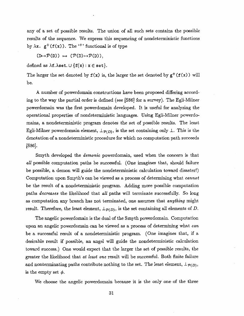
any of a set of possible results. The union of all such sets contains the possible
results of the sequence. We express this sequencing of nondeterministic functions
by ..\x. g+(f(x)). The •+' functional is of type
(Do-+P (D) ) 1-+ ('P (D) >-+'P (D) ) ,
defined as ..\f . ..\set. U {f(x): x E set}.
The larger the set denoted by f (x) is, the larger the set denoted by g+ (f (x)) will
be.
A number of powerdomain constructions have been proposed differing accord
ing to the way the partial order is defined (see [S86] for a survey). The Egli-Milner
powerdornain was the first powerdomain developed. It is useful for analyzing the
operational properties of nondeterministic languages. Using Egli-Milner powerdo
mains, a nondeterministic program denotes the set of possible results. The least
Egli-Milner powerdomain element, .l'P(D), is the set containing only .l. This is the
denotation of a nondeterministic procedure for which no computation path succeeds
[S86].
Smyth developed the demonic powerdornain, used when the concern is that
all possible computation paths be successful. (One imagines that, should failure
be possible, a demon will guide the nondeterministic calculation toward disaster!)
Computation upon Smyth's can be viewed as a process of determining what cannot
be the result of a nondeterministic program. Adding more possible computation
paths decreaJes the likelihood that all paths will terminate successfully. So long
as computation any branch has not terminated, one assumes that anything might
result. Therefore, the least element, .lp(D), is the set containing all elements of D.
The angelic powerdomain is the dual of the Smyth powerdomain. Computation
upon an angelic powerdornain can be viewed as a process of determining what can
be a successful result of a nondeterministic program. (One imagines that, if a
desirable result if possible, an angel will guide the nondeterministic calculation
toward success.) One would expect that the larger the set of possible results, the
greater the likelihood that at least one result will be successful. Both finite failure
and nonterminating paths contribute nothing to the set. The least element, .l'P(D),
is the empty set ¢>.
We choose the angelic powerdomain because it is the only one of the three
31

containing the empty set as an element (the denotational equations which follow
make use of</>). That the angelic powerdomain is the correct choice for a language
combining functional and logic programming can be seen by considering the seman
tics of Horn logic programming. In an attempt to find values for the goal's logical
variables so as to make the goal true, a Horn logic interpreter nondeterministi
cally chooses a logical derivation using the program clauses from among all possible
derivations. The set of solutions contains the results of the successful derivations;
the derivations which fail or diverge add nothing to the set. If all derivations fail
or diverge, the set of solutions is empty. If we view the set of all answer substitu
tions as a domain D, and the set of correct answer substitutions as an element of
'P( D), it is clear that we want ..L'P(D) to be t/>. Since a description of Horn logic in
terms of powerdomains would use the angelic powerdomain, it seems clear that set
abstraction for the purpose of incorporating logic programming capabilities should
also be described via this powerdomain construction.
We would like to have a partial order on sets which exhibits the property that
a set becomes more defined as one adds new elements, and that it also becomes
more defined as the elements within become more defined (according to the partial
order of the base domain). We would like to be able to say that for two sets A
and B, if for all a E A there exists a b E B such that a l;v b, then A I;'P(D) B.
However, this is not a partial order, as this would equate {dbd2 } with {d2 } when
d1 C d2. Yet, though these sets are distinct, they are computationally equivalent
(because the angel always chooses the best possible result). So theoretically, we are
working not with sets, but with equivalence classes of sets. Furthermore, the need
for continuity requires that for any chain of elements t; E D,
where singleton set { t;} actually represents the equivalence class of sets containing
that singleton set. These requirements motivate the following definitions (taken
from [S86]).
Definition 3.18: A Scott-topology upon a domain 0 is a collection of subsets
of 0 known as open sets. A set U <; 0 is open on the Scott-topology iff:
32

1) U is closed upwards, that is, for every d2 E D, if there exists a d 1 E U such that
d1 C d2, then d2 E U; and
2) If d E U is the least upper bound of a chain C in D, then some cEDis in U.
Definition 3.19: The symbol r;~, pronounced 'less defined than or equivalent
to', is a relation between sets. For A, B <; D, we say that A r;~ B iff for every a E A
and open set U <; D, if a E U then there exists a b E B such that b E U also.
Definition 3.20: We say A RJ B iff both A r;~ B and B C~ A. We denote the
equivalence class containing A as [A]. This class contains all sets B <; D such that
A~B.
We define the partial order on equivalence classes as: [A] C [B] iff A r;_ B. For
domain D, the powerdomain of D, written P(D), is the set of equivalence classes,
each member of an equivalence class being a subset of D.
Theorem 3.4 (Schmidt [S86]): The following operations are continuous:
,P: P (D) denotes [ {}] . This is the least element.
{-}: D >-+ 'P(D) maps d E D to [{d}].
_U_: P(D) xP(D)>-+P(D) maps [A] U [B] to [AU B].
+: (D~->'P(D)) ,__. ('P(D)~->'P(D)) is ..\L\(A].(U{f(a): a E A}].
An example will provide intuition about the use of •+•. Suppose we have a set
S = {1, 2, 3}, and we wish to create a new set, each element of which is of the
form f(x) where xis inS. Then
(.Ax. {f(x)})+({1,2,3}) = {f(1),j(2),j(3)}.
In this work we use a noncurried variation of •+•, that is, we use it as a primitive
function of type
((D~->'P(D)) X P(D)) 1-> 'P(D).
This function is strict in its second argument.
3.3 Denotational Semantics of PowerFuL
This section gives the semantics of PowerFuL using the concepts reviewed
above. After defining the domain of data objects which can be represented in
PowerFuL, we provide a function which shows the way a PowerFuL program can
33
be mapped onto this domain. The semantic primitives used are, for the most part,
quite conventional. However, a few unusual primitives, (called coercions) will be
discussed in a special section.
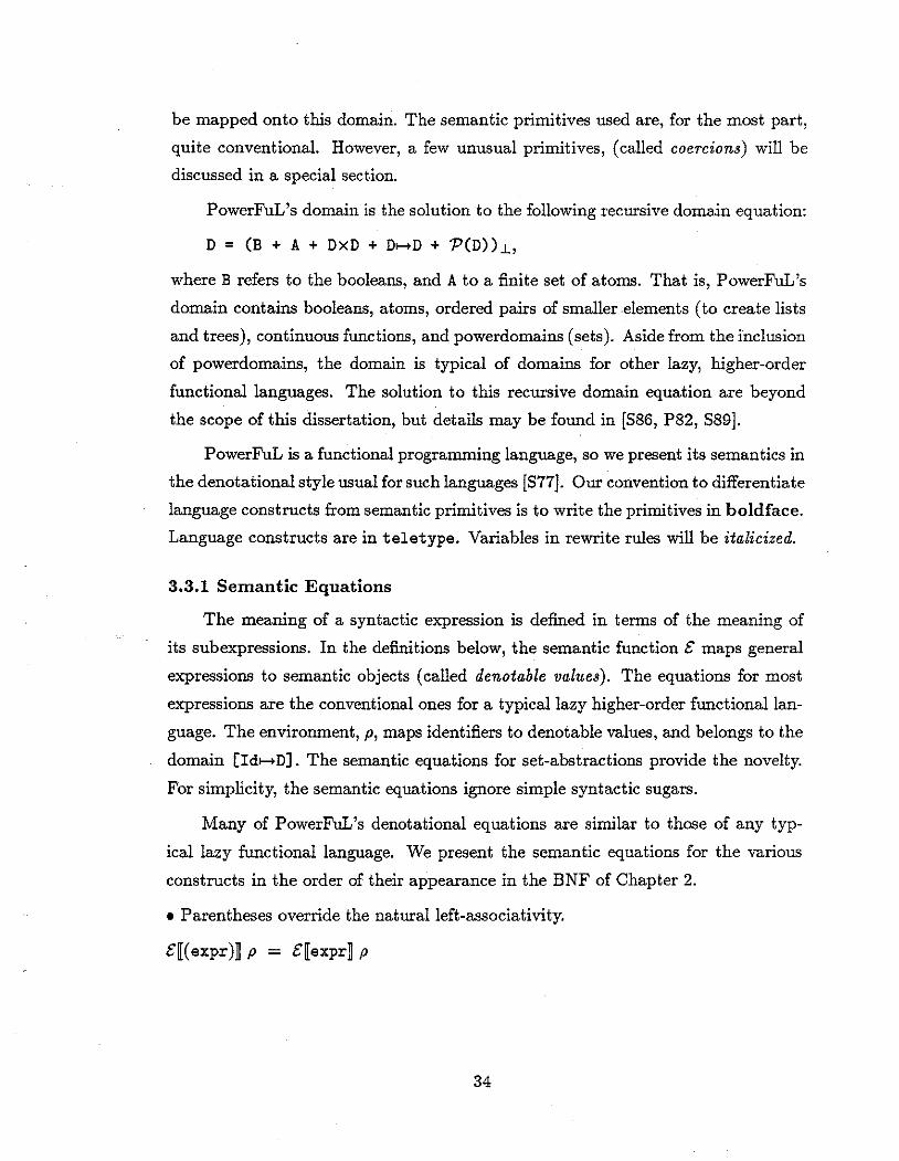
PowerFuL's domain is the solution to the following recursive domain equation:
D = (B + A + DxD + D>->D + "P(D)).L,
where B refers to the booleans, and A to a finite set of atoms. That is, PowerFuL's
domain contains booleans, atoms, ordered pairs of smaller elements (to create lists
and trees), continuous functions, and powerdomains (sets). Aside from the inclusion
of powerdomains, the domain is typical of domains for other lazy, higher-order
functional languages. The solution to this recursive domain equation are beyond
the scope of this dissertation, but details may be found in [S86, P82, S89].
PowerFuL is a functional programming language, so we present its semantics in
the denotational style usual for such languages [S77]. Our convention to differentiate
language constructs from semantic primitives is to write the primitives in boldface.
Language constructs are in teletype. Variables in rewrite rules will be italicized.
3.3.1 Semantic Equations
The meaning of a syntactic expression is defined in terms of the meaning of
its subexpressions. In the definitions below, the semantic function E maps general
expressions to semantic objects (called denotable values). The equations for most
expressions are the conventional ones for a typical lazy higher-order functional lan
guage. The environment, p, maps identifiers to denotable values, and belongs to the
domain [Id>->D]. The semantic equations for set-abstractions provide the novelty.
For simplicity, the semantic equations ignore simple syntactic sugars.
Many of PowerFuL's denotational equations are similar to those of any typ
ical lazy functional language. We present the semantic equations for the various
constructs in the order of their appearance in the BNF of Chapter 2.
• Parentheses override the natural left-associativity.
£[( expr)] p = E[expr] p
34
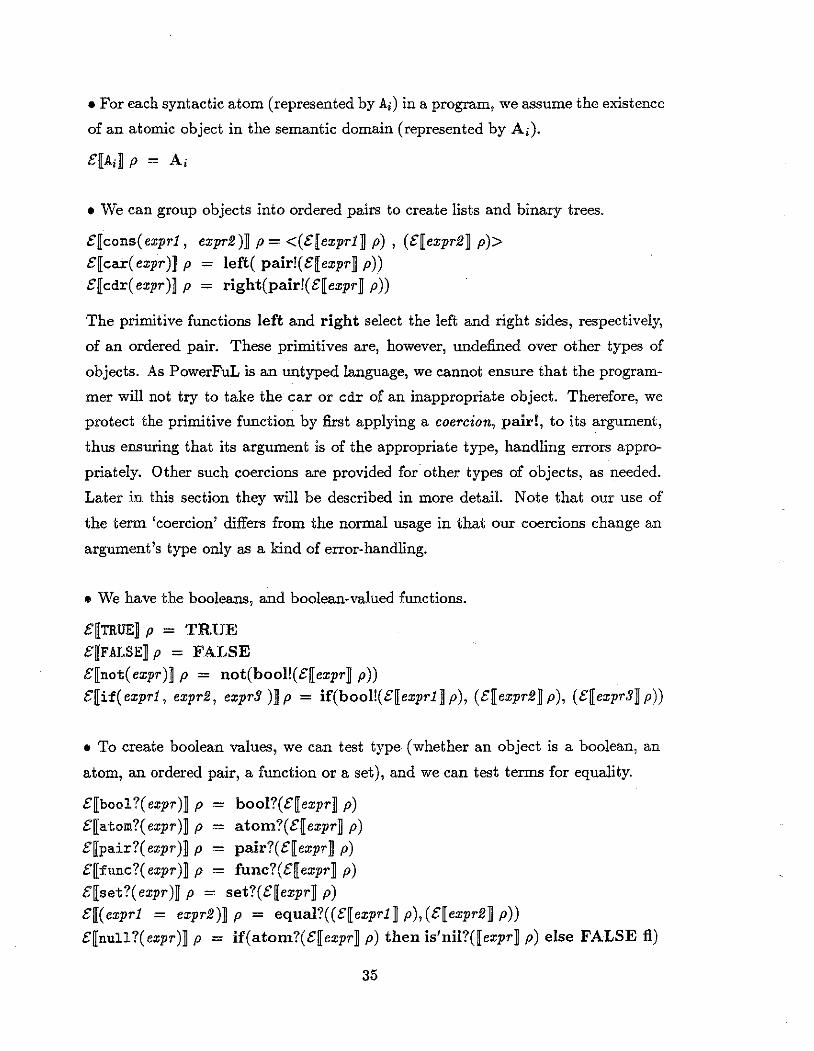
• For each syntactic atom (represented by A;) in a program, we assume the existence
of an atomic object in the semantic domain (represented by A;).
t'[A;] p = A;
• We can group objects into ordered pairs to create lists and binary trees.
t'[cons(exprt, expr2)] p = <(t'[expr1] p), (E[expr2] p)> t'[car(expr)] p - left( pair!(t'[expr] p)) £[cdr( expr)] p = right(pair!(t'[expr] p))
The primitive functions left and right select the left and right sides, respectively,
of an ordered pair. These primitives are, however, undefined over other types of
objects. As PowerFuL is an untyped language, we cannot ensure that the program
mer will not try to take the car or cdr of an inappropriate object. Therefore, we
protect the primitive function by first applying a coercion, pair!, to its argument,
thus ensuring that its argument is of the appropriate type, handling errors appro
priately. Other such coercions are provided for other types of objects, as needed.
Later in this section they will be described in more detail. Note that our use of
the term 'coercion' differs from the normal usage in that our coercions change an
argument's type only as a kind of error-handling.
e We have the booleans, and boolean-valued functions.
£[TRUE] p = TRUE e[F ALSE] p = FALSE e[not(expr)] p = not(bool!(t'[expr] p)) £[if( exprt, expr2, expr3 )] p = if(bool!(t'[exprt] p), (e[expr2] p), (e[expr3] p))
• To create boolean values, we can test type (whether an object is a boolean, an
atom, an ordered pair, a function or a set), and we can test terms for equality.
t'[bool?(expr)] p - bool?(t'[expr] p)
e[atom?(expr)] p - atom?(t'[expr] p) E[pair?(expr)] p - pair?(t'[expr] p)
f[func?(expr)] p - func?(f[expr] p)
t'[set?(expr)] p = set?(e[expr] p) t'[(exprt = expr2)] p = equal?((E[exprt] p),(t'[expr2] p))
t'[null?(expr)] p = if(atom?(t'[expr] p) then is'nil?([expr] p) else FALSE fi)
35

The equality predicate can compare booleans, atoms, and, provided it can compare
the respective subtrees, ordered pairs. It does not attempt to compare sets or
functions for equality (if you try, it returns ..L). Applied to two first-order infinite
lists, it returns FALSE if they differ, but fails to terminate (returns ..L) when they
are identical. A conventional operation tests whether a "list" is empty (i.e. equals
the atom 'nil).
• We can look up identifiers in the environment, and also create new bindings.
£[identifier~ p = p( identifier) £[letrec defs in expression] p = £[expression~ (:D[defs~ p) V[id be expr~ p = p[.:FIX(.A X. (£[expr~ p[X/id]))jid]
V[id be expr, defs] p = (V[defs~ p) [:FIX(,\ X. (E[expr~ (V[defs] p[X /id])))/id]
In the above equations, :FIX computes the least fixpoint of a functional.
Rather than using the fixpoint operator as a primitive, we can define it via:
:FIX(!) = f(.:FIX(f))
Taken as an equation, the above is true if :FIX computes any fixpoint of its ar
gument. But taken as a recursive definition with Definition 3.17 in mind, :FIX is
taken to be the least fixpoint of the functional .AF. ,\f. f(F(f)). Using Theorem
3.2, this can be shown to equal .Af. lfp(f).
• We can create functions through lambda abstraction, and apply functions to their
arguments.
£[.Aid. expr] p = .Ax. (£[expr] p[xjid]) £[expr1 expr2] p = func!(£[expr1~ p)(£[expr2] p)
In the above equations, we considered only functions of one argument. A function of
multiple arguments can be considered syntactic sugar either for a curried function,
or for a function whose single argument is a list.
• To build sets, the user begins with the empty set, and singleton sets, each con
structed from an element of the powerdomain's base domain. The union operation
builds larger sets from smaller ones.
36
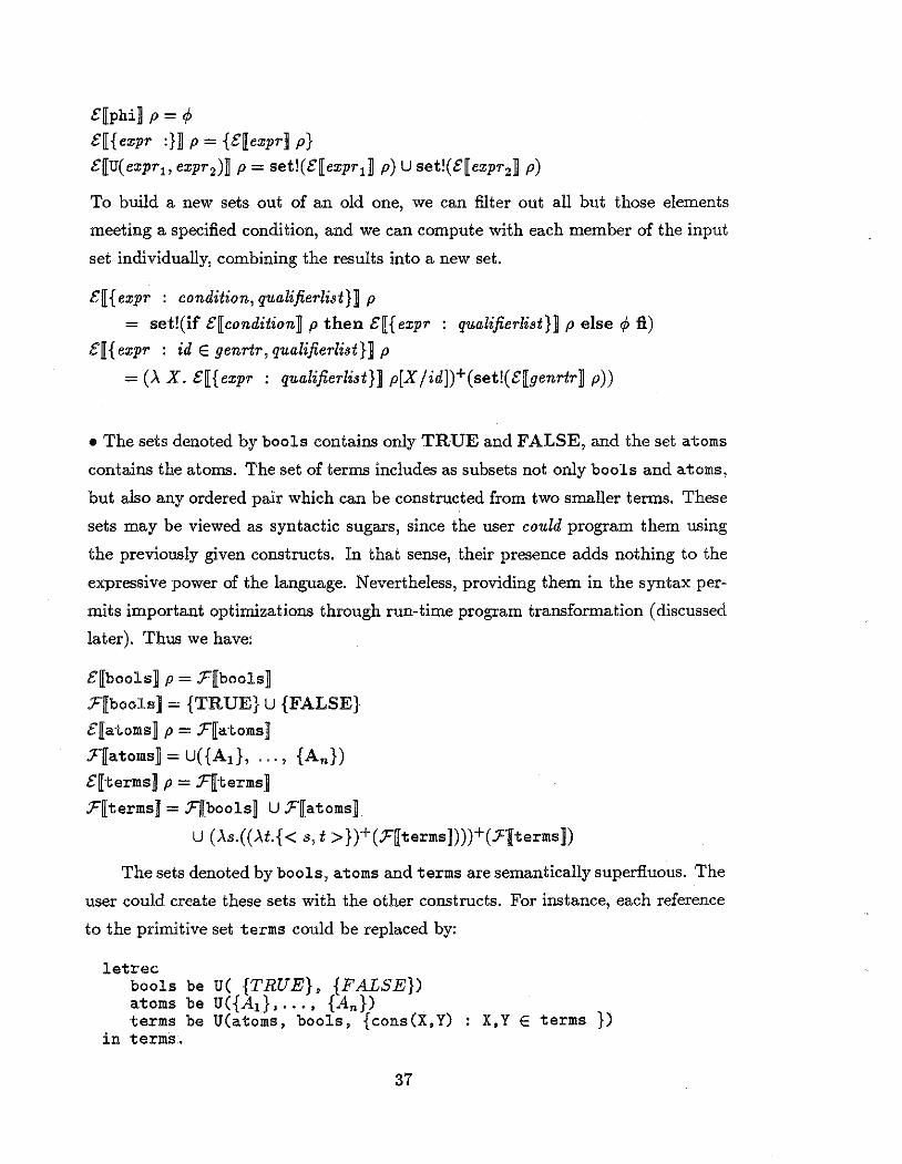
£[phi] p = 1>
E[{expr :}] p = {E[expr] p}
E[U(expr1 , expr2)] p = set!(E[expr1 ] p) U set!(E[expr2 ] p)
To build a new sets out of an old one, we can filter out all but those elements
meeting a specified condition, and we can compute with each member of the input
set individually, combining the results into a new set.
E[{ expr : condition, qualifierlist}] p
= set!(if £[condition] p then£[{ expr : qualifierlist}] p else </>fl.) £[ { expr : id E genrtr, qualifierlist}] p
=(>.X. E[{expr : qualifierlist}] p[X/id])+(set!(E[genrtr] p))
• The sets denoted by bools contains only TRUE and FALSE, and the set atoms
contains the atoms. The set of terms includes as subsets not only bools and atoms,
but also any ordered pair which can be constructed from two smaller terms. These
sets may be viewed as syntactic sugars, since the user could program them using
the previously given constructs. In that sense, their presence adds nothing to the
expressive power of the language. Nevertheless, providing them in the syntax per
mits important optimizations through run-time program transformation (discussed
later). Thus we have:
E[bools] p = .F[bools]
.F[bools] ={TRUE} u {FALSE}
£[atoms] p = .F[atoms]
.F[atoms]=U({AI}, ... ,{An})
£[terms] p = .F[terms]
.?="[terms]= .F[bools] U .F[atoms]
U (>.s.((>.t.{< s,t >})+(.F[terms])))+(.F[terms])
The sets denoted by bools, atoms and terms are semantically superfluous. The
user could create these sets with the other constructs. For instance, each reference
to the primitive set terms could be replaced by:
letrec bools atoms terms
in terms.
be be be
U( {TRUE}, {FALSE}) U({AI}, ... , {An}) U(atoms, bools, {cons(X,Y)
37
X,Y E terms })
PowerFuL provides these sets as primitives, so the interpreter can recognize them
and treat their enumerated variables as logical variables, for greater efficiency. This
will be discussed in greater detail in Chapter 6.
The functions £, 'D, :F and :FIX are mutually recursive. Their meaning is
the least fixed point of the recursive definition. This fixed-point exists because we
have combined continuous primitives with continuous combinators. Most of these
primitives are fairly standard, and will be described in a later section. Note the use
of the primitive •+• (for distributing elements of a powerdomain to a function) in
defining the meaning of the set abstraction construct.
3.3.2 Coercions
A few words must be said about some other novel primitives, here called coer
cions. Most primitives are only defined over portions of the domain D. The boolean
operators are only defined over B.L; the operations left and right assume the argu
ments to be ordered pairs; function application (,8-reduction) is defined only when
the left argument is in fact a lambda expression; and only sets can contribute to a
set union.
Five primitives coerce inappropriate arguments to the least-defined object of
the appropriate type. The are listed below. bool!: D >-+ B .L
atom!: D >-+ A.L
pair!: D >-+ DxD func!: D >-+ [D>-+D] set!: D >-+ 'P(D)
The function bool! maps TRUE and FALSE to themselves, and otherwise maps
arg to j_ . The function atom! maps arg to itself if arg is an atom, and maps arg to
j_ otherwise. The function pair! maps arg to itself if arg is a member of DxD, and
to j_DxD (that is, < j_, j_ >) otherwise. The function func! maps arg to itself if
arg is a member ofD>-+D and to j_DxD (that is, .Ax. j_) otherwise. The function set!
maps arg to itself if arg is a member of 'P(D) and to j_.P(D) (that is, ¢)otherwise.
The coercions ensure that primitives handles inappropriate input reasonably.
For instance, the union constructor is appropriately applied only to sets. If the
argument is something other than as set (perhaps j_), then this input is treated as
the empty set. This make sense because
38

1) only sets contain elements- other objects do not;
2) a set is completely defined by the elements it contains; and
3) the empty set is the only set not containing any elements.
Thus, the expression U(' a, expr) denotes a set containing 'a, regardless of whether
or not expr can be computed . .This is analogous the the set of solutions to a Horn
logic program and goal, the elements of which are determined by successful deriva
tions (or refutations), ignoring derivations which fail or diverge. For uniformity,
we define analogous coercions to handle similar questions about primitives of other
types.
Theorem 3.5: The coercion set! is continuous.
Proof: We will prove the continuity of setL Consider a chain of objects from
domain D: to, t1, t2, ... , such that fori< j, t;!:::; fj. If there is no i such that t; is
in 'P(D), then for all i, by definition, set!( t;) = _LP(D) = ¢. Furthermore, U; t;
will not be in P(D), so by definition,
set!(U; t;) = ¢.
Thus we have,
U; set!(t;) = ¢ = set!(U; t;),
proving continuity for that case. The only other possibility is that the sequence
does converge to a powerdomain element. In that case, let tk be the first member
of the chain in 'P(D). for any i < k, t; can only equal -lv, so set!(t;) equals¢, by
definition. Fori 2: k, set!(t;) equals t;, also by definition. Therefore,
U; set!(t;) = Ui~k set!(t;)
- ui~k t;
- set!(U;~k t;)
- set!(U; t;).
Hence, set! is continuous. End of Proof
Proofs of the continuity of the other coercions are similar.
3.4 Summary
In this chapter we described the semantic domain of PowerFuL. It resembles
the recursively defined domains of ordinary untyped functional languages, in which
39
complex objects are built from simpler objects via sequencing constructors (ordered
pairs) and function definition. What is new is the use of powerdomain constructors
to build sets. We gave the rationale for chosing angelic powerdomains, rather than
one of the other types of powerdomains.
The semantic equations for the traditional features are unaffected by the enrich
ment of the domain. All that was needed to handle set abstraction is the addition of
a few new equations. We consider this to be the strongest testimony of the elegance
of this approach.
The primitive functions used in the semantic equations are defined in the next
chapter. The use of coercions permits simpler definitions of primitives, as we need be
concerned only with appropriate subsets of PowerFuL's domain; redundant descrip
tions of "error handling" is avoided. This will be especially helpful when describing
the operational semantics, and its relation to the denotational semantics, in the
next chapter.
40

4 FROM DENOTATIONAL TO OPERATIONAL SEMANTICS
Though the denotational semantics usually provides the clearest and simplest
definition of the syntactic constructs, an operational semantics is essential if the
language is to be implemented. Therefore, even those defining a language via de
notational semantics usually also provide an operational definition. In such cases,
one would like to know the extent to which the two semantics agree. A proof of
equivalence is rarely given; usually the operational semantics are incomplete when
computing infinite objects f. Though Horn logic makes for a very simple language
(simple flat domain and only two types of clauses) the proof of correctness is far
from trivial [VK76]. The task becomes more difficult as the operational semantics
becomes low-level (hardware-oriented). The closer to the denotational definition
the operational semantics remains, the easier this proof should be. Therefore, in
the remaining chapters, we devise an operational procedure from the denotational
equations directly. This ensures that our operational semantics is consistent with
respect to the denotational definitions; in this chapter we also speculate upon its
completeness.
The semantic equations provided in the last chapter are a recursive definition
of the semantic function£, which maps PowerFuL programs into objects from the
semantic domain (the value denoted by the program). Assuming that the primitive
functions are continuous, the recursive equations define a functional which has a
least fixpoint, which can be "computed" by taking successive approximations, as
alluded to in Chapter 3. This fixpoint is taken to be the value of£. A procedure to
execute £ on its input is, by definition, an interpreter for the PowerFuL language.
In this section we examine ways of executing the function £ when applied to a
PowerFuL program and an (initially empty) environment. Given implementations
t This issue is discussed further in section 4.4.1.
for the semantic primitives (provided in the next chapter) and the ability to reduce
lambda-expressions, a computation rule is all that is needed to convert the semantic
equations into an interpreter. If the computation rule is a fixpoint rule, then the
computed result will indeed equal the fixpoint value of t'[program] A ('A' stands
for the empty environment). In other words, we interpret the language of denota
tional semantics as a functional programming language in its own right, not merely
reading it as a pseudocode. Since a functional program has both a declarative and
an operational reading, the denotational equations will thus provide both the deno
tational semantics of PowerFuL, and also a simple interpreter consistent with the
declarative reading.
To illustrate our approach, suppose that we wish to evaluate the expression:
car( cons( cons('a,'b), 'a))
The denotational equations for translating syntactic symbols of atoms to real atoms
in the semantic domain (differentiated here by the type font), and semantic equa
tions for cons, car and cdr are as follows:
t'[A;] p = A; t'[cons(expr1, expr2)] p = <(t'[expr1] p), (t'[expr2] p)> t'[ car( expr)] p - left( pair!( t'[ expr] p)) t'[cdr(expr)] p = right(pair!(t'[expr] p))
The rewrite rules to implement the semantic primitives left and right are:
left( <1st, 2nd>) = 1st right(<1st, 2nd>) = 2nd
The denotational equations map syntactic constructs to semantic constructs,
and the semantic primitives map semantic objects onto other semantic objects. In
this case, both kinds of mappings are defined through rewrite rules. We wish to
find the semantic object denoted by the syntactic expression above. That is, we
wish to compute:
t'[car(cons(cons('a,'b),' a))] A.
Using the semantic equation for car, we rewrite the above expression to:
left t'[cons(cons('a,'b),'a)] A.
We do not yet have enough information to apply the rewrite rule for left, so we
must translate more syntax using the semantic equation for cons, and will then
42
obtain:
left < E[cons('a,'b)] A, E['a] A>·
We now have enough information to execute the semantic primitive left, and will
get:
E[cons('a,'b)] A.
Further rewriting with the semantic equations produces the final value:
<'a, 'b >.
Thus, we see that one can sometimes execute a program directly from the denota
tional semantic equations.
The remainder of this chapter provides a more rigorous development of this
technique. The basic ideas come from Vuil!ernin's pioneering work on correct im
plementation of recursive programs [V74]. Following Kleene, Vuillernin views the
meaning of a recursive definition to be the least fixpoint of an associated functional.
As the fixpoint is shown to be the least upper bound of a (possibly infinite) chain of
approximations, computation becomes synonymous with the production of better
and better approximations. Usually, there are several places in an approximation
where one can seek improvement. The computation rule chooses which of these
places to work on next. Vuillernin provides conditions under which the successive
approximations will converge toward the value implicitly given by the fixpoint defi
nition. We then apply these ideas to PowerFuL's denotational equations, a recursive
definition in its own right, to produce our operational semantics.
4.1 Recursion and Least Fixpoints
Consider a recursive definition of the form:
F(x) = r[F](x)
for function F, where r is a functional over D1 x ... x Dn 1-+ D, expressed by
composing a term from:
a) the individual variables x =< x1, x2, ... , Xn >;
b) known monotonic and continuous functions, called primitives; and
c) the function variable, F.
43
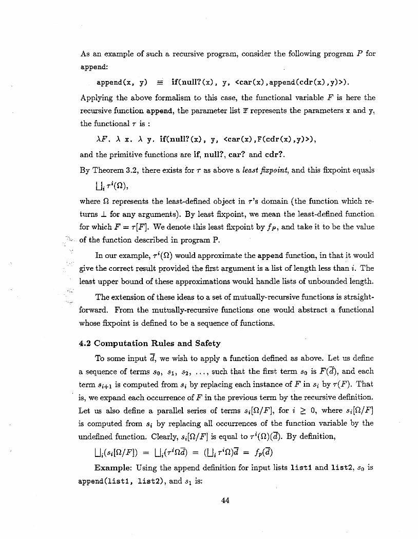
As an example of such a recursive program, consider the following program P for
append:
append(x, y) if(null?(x), y, <car(x) ,append(cdr(x) ,y)>).
Applying the above formalism to this case, the functional variable F is here the
recursive function append, the parameter list x represents the parameters x andy,
the functional T is :
>..F. >.. x. >.. y. if(null?(x), y, <car(x) ,F(cdr(x) ,y)>),
and the primitive functions are if, null?, car? and cdr?.
By Theorem 3.2, there exists for T as above a least fixpoint, and this fixpoint equals
where f! represents the least-defined object in r's domain (the function which re
turns .l for any arguments). By least fixpoint, we mean the least-defined function
for which F = r[F]. We denote this least fixpoint by fp, and take it to be the value
of the function described in program P.
In our example, ri(f!) would approximate the append function, in that it would
give the correct result provided the first argument is a list of length less than i. The
least upper bound of these approximations would handle lists of unbounded length.
The extension of these ideas to a set of mutually-recursive functions is straight
forward. From the mutually-recursive functions one would abstract a functional
whose fixpoint is defined to be a sequence of functions.
4.2 Computation Rules and Safety
To some input d, we wish to apply a function defined as above. Let us define
a sequence of terms s0 , 81, s2 , ••• , such that the first term so is F(d), and each
term 8;+J is computed from s; by replacing each instance ofF ins; by r(F). That
is, we expand each occurrence ofF in the previous term by the recursive definition.
Let us also define a parallel series of terms 8;[!1/ F], for i 2:: 0, where s;[fl/ F]
is computed from 8; by replacing all occurrences of the function variable by the
undefined function. Clearly, 8;[!1/ F] is equal to ri(f!)(d). By definition,
U;(8;[f!/F]) = U;(r;f!d) = (U;rif!)d = /p(d)
Example: Using the append definition for input lists list1 and list2, so is
append(list1, list2), and 8 1 is:
44

if(null?(listl), list2, <car(listl),append(cdr(listl),list2)>).
We can keep expanding the occurrences of append to any depth. The sequence of
approximations begins with s 0 (!2/F], which is Q(listl, list2) (i.e . ..L), followed
by s 1 (!2/F], which is:
if( null? (listl), list2, <car(listl) ,n(cdr(list1) ,list2) >).
In this case, there is only one occurrence of the recursive function to expand
at each step. In general there may be more. Let us define a new series t; similar to
s;, where t 0 = s0 = F(d), but where each t;+l is computed from t; by expanding
only some of the occurrences of F in t;, instead of all.
Definition 4.1: A computation rule C tells us which occurrences of F(e) should
be replaced by r(F](e) in each step.
For each t;, we compute t;[Qj F] in the same way we computed s;[Qj F] from
Si.
Theorem 4.1 (Cadiou (V74]): For any computation rule C,
Proof: For any i, t;[f!/ F]!;;; s;[Qj F], and therefore
U;( t;[nj F]) !;;; U;(s;(!2/ F]) = /p(d).
End of Proof
Definition 4.2: A computation rule is said to be a fixpoint computation rule for
program P if for all d in the relevant domain,
Vuillemin gives a condition which, if satisfied, means that a computation rule is a
fixpoint rule. To explain this condition, we need a bit more notation.
Definition 4.3: A substitution step expands some or all occurrences of the
recursive function calls in the term. Given a term t;, let Fy represent the occurrences
of F which the computation rule would choose, and let Fn represent those which
would not be chosen for expansion in the next step. Let
represent the result of replacing all chosen occurrences by S, and the unchosen by
T. Then
45

is just t;, and
is the same as
t;[f2/ F].
Let
represent the result computed if the chosen occurrences were never expanded, but
all other occurrences expanded arbitrarily far.
Definition 4.4: A safe substitution step chooses Fy so that
Intuitively, the computation is safe if the occurrences chosen are so important that,
were these never expanded, no other expansions would matter.
Definition 4.5: A computation rule is safe if it provides for only safe substitution
steps.
Theorem 4.2 (Vuillemin [V74]): If the computation rule used in producing the
series v; is a safe, then
To summarize the proof, we note that the fixpoint is equal to the least upper
bound of approximations made by the full-substitution rule. We need only show
that for each approximation made by the full-substitution rule, a safe rule will
produce an approximation that is at least as good. Each approximation using the
full-substitution rule expands only a finite number of occurrences. If we perform
that many safe substitution steps, then either we will have expanded all of these
(guaranteeing a suitably good approximation), or we will have had one or more steps
in which none of the remaining occurrences expanded with the full-substitution
rule were chosen. When that happens, the safety condition shows that the full
substitution approximation cannot be any better.
Using Theorems 4.1 and 4.2, then for any safe computation rule,
46
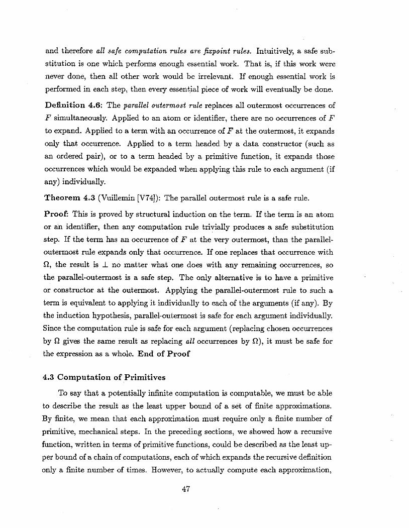
and therefore all safe computation rules are fixpoint rules. Intuitively, a safe sub
stitution is one which performs enough essential work. That is, if this work were
never done, then all other work would be irrelevant. If enough essential work is
performed in each step, then every essential piece of work will eventually be done.
Definition 4.6: The parallel outermost rule replaces all outermost occurrences of
F simultaneously. Applied to an atom or identifier, there are no occurrences ofF
to expand. Applied to a term with an occurrence ofF at the outermost, it expands
only that occurrence. Applied to a term headed by a data constructor (such as
an ordered pair), or to a term headed by a primitive function, it expands those
occurrences which would be expanded when applying this rule to each argument (if
any) individually.
Theorem 4.3 (Vuillemin (V74]): The parallel outermost rule is a safe rule.
Proof: This is proved by structural induction on the term. If the term is an atom
or an identifier, then any computation rule trivially produces a safe substitution
step. If the term has an occurrence ofF at the very outermost, than the parallel
outermost rule expands only that occurrence. If one replaces that occurrence with
n, the result is .l no matter what one does with any remaining occurrences, so
the parallel-outermost is a safe step. The only alternative is to have a primitive
or constructor at the outermost. Applying the parallel-outermost rule to such a
term is equivalent to applying it individually to each of the arguments (if any). By
the induction hypothesis, parallel-outermost is safe for each argument individually.
Since the computation rule is safe for each argument (replacing chosen occurrences
by n gives the same result as replacing all occurrences by !1), it must be safe for
the expression as a whole. End of Proof
4.3 Computation of Primitives
To say that a potentially infinite computation is computable, we must be able
to describe the result as the least upper bound of a set of finite approximations.
By finite, we mean that each approximation must require only a finite number of
primitive, mechanical steps. In the preceding sections, we showed how a recursive
function, written in terms of primitive functions, could be described as the least up
per bound of a chain of computations, each of which expands the recursive definition
only a finite number of times. However, to actually compute each approximation,
47
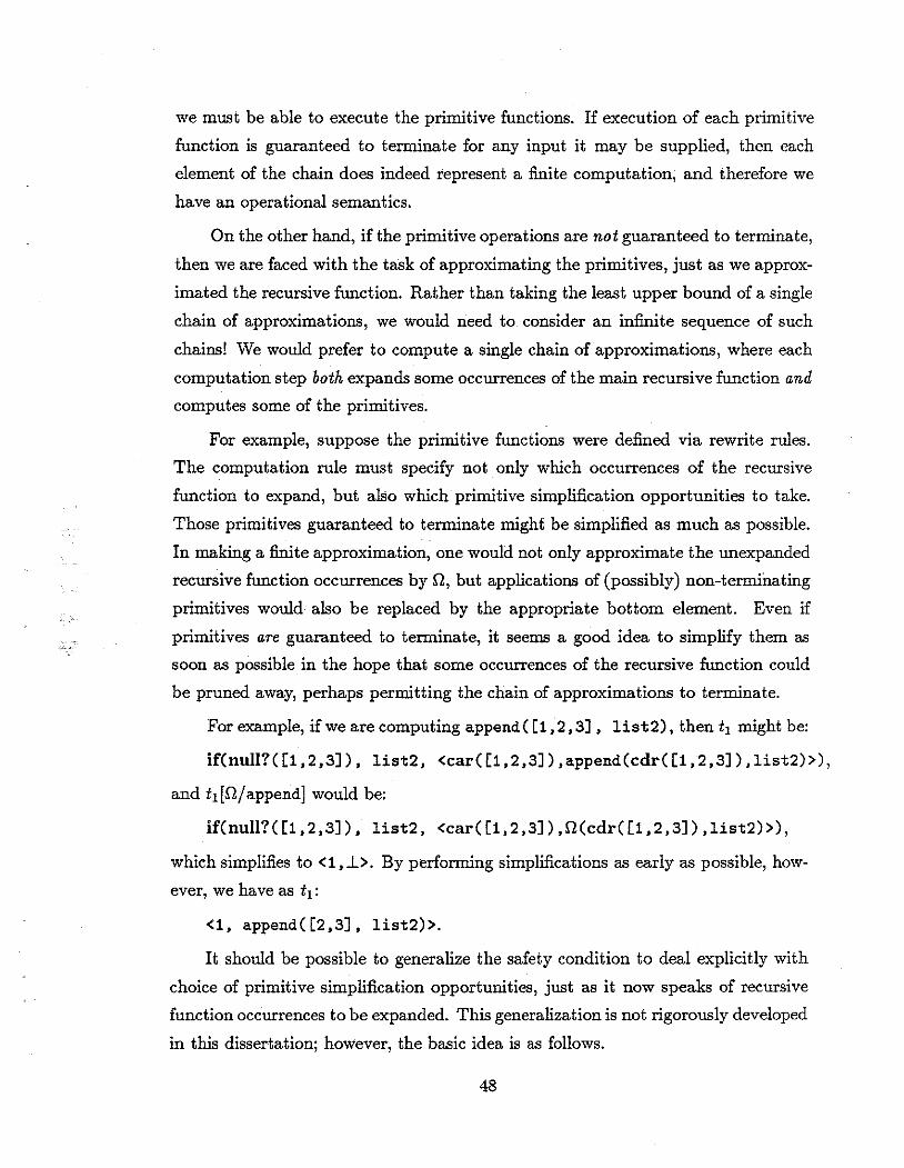
we must be able to execute the primitive functions. If execution of each primitive
function is guaranteed to terminate for any input it may be supplied, then each
element of the chain does indeed represent a finite computation, and therefore we
have an operational semantics.
On the other hand, if the primitive operations are not guaranteed to terminate,
then we are faced with the task of approximating the primitives, just as we approx
imated the recursive function. Rather than taking the least upper bound of a single
chain of approximations, we would need to consider an infinite sequence of such
chains! We would prefer to compute a single chain of approximations, where each
computation step both expands some occurrences of the main recursive function and
computes some of the primitives.
For example, suppose the primitive functions were defined via rewrite rules.
The computation rule must specify not only which occurrences of the recursive
function to expand, but also which primitive simplification opportunities to take.
Those primitives guaranteed to terminate might be simplified as much as possible.
In making a finite approximation, one would not only approximate the unexpanded
recursive function occurrences by n, but applications of (possibly) non-terminating
primitives would also be replaced by the appropriate bottom element. Even if
primitives are guaranteed to terminate, it seems a good idea to simplify them as
soon as possible in the hope that some occurrences of the recursive function could
be pruned away, perhaps permitting the chain of approximations to terminate.
For example, if we are computing append ( [1, 2, 3] , list2), then t 1 might be:
if( null?( [1, 2 ,3]), list2, <car( [1, 2 ,3]) ,append(cdr( [1, 2 ,3]), list2) >),
and t1 [i1/append] would be:
if( null?( [1, 2 ,3]), list2, <car( [1, 2 ,3]) ,Q(cdr( [1, 2, 3]), list2) >),
which simplifies to <1,..L>. By performing simplifications as early as possible, how
ever, we have as t1 :
<1, append([2,3], list2)>.
It should be possible to generalize the safety condition to deal explicitly with
choice of primitive simplification opportunities, just as it now speaks of recursive
function occurrences to be expanded. This generalization is not rigorously developed
in this dissertation; however, the basic idea is as follows.
48

The notation for approximating the current term, t;[fl/ F] would now mean that
we replace not only applications of the recursive function( s) by the appropriately
typed undefined element, but we do the same for uncomputed applications of the
primitives. The safety condition,
now would state that a computation step is safe if, among those recursive-function
occurrences to be expanded and those primitive applications to be simplified, are
some so critical that, were these operations never done, the current approximation
could never be improved upon no matter how much computation elsewhere were
performed. This means, for any part of t; which is not yet fully computed, the
computation rule has chosen vital steps to perform. We may say that such a safe
computation step is fair, because it simultaneously does work necessary for each
incomplete part the result being computed (it may do some unnecessary work as
well, but this does not concern us).
This is not to say that the occurrences chosen by the safe computation rule
must be expanded immediately for convergence; the order in which necessary work
is performed ought not affect convergence (though speed of convergence might be
affected). For any approximation requiring only a finite amount of computation (a
finite number of recursive function expansions and a finite number of primitive sim
plifications), any safe computation rule should eventually produce an approximation
that is at least as good.
One might question the claim that, in producing a finite approximation, the
order in which necessary work is performed is irrelevant. After all, are not some
computation rules more powerful than others? Does not the innermost computation
rule sometimes fails to converge, where outermost evaluation succeeds? The key
word here is necessary. An innermost computation rule may fail to converge if none
of the steps necessary to compute some part of the denoted object are ever chosen.
Instead, the innermost computation rule might put all its effort into computing an
infinite subexpression whose computation is unnecessary to the main result.
Since any computable function can be viewed as the least upper bound of a
set of finite approximations, and since a safe computation rule should be able to
produce a finite approximation at least as good as any of them, we believe that
49
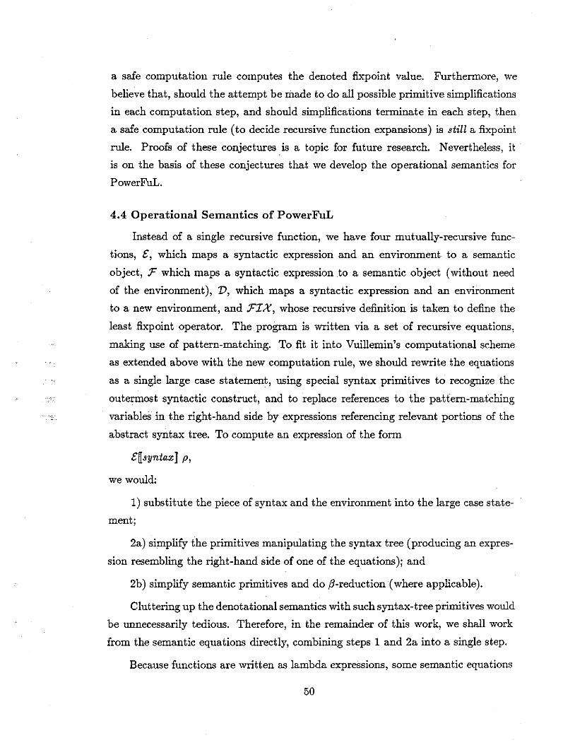
a safe computation rule computes the denoted fixpoint value. Furthermore, we
believe that, should the attempt be made to do all possible primitive simplifications
in each computation step, and should simplifications terminate in each step, then
a safe computation rule (to decide recursive function expansions) is still a fixpoint
rule. Proofs of these conjectures. is a topic for future research. Nevertheless, it
is on the basis of these conjectures that we develop the operational semantics for
PowerFuL.
4.4 Operational Semantics of PowerFuL
Instead of a single recursive function, we have four mutually-recursive func
tions, e, which maps a syntactic expression and an environment to a semantic
object, :F which maps a syntactic expression to a semantic object (without need
of the environment), TJ, which maps a syntactic expression and an environment
to a new environment, and :FIX, whose recursive definition is taken to define the
least fixpoint operator. The program is written via a set of recursive equations,
making use of pattern-matching. To fit it into Vuillemin's computational scheme
as extended above with the new computation rule, we should rewrite the equations
as a single large case statement, using special syntax primitives to recognize the
outermost syntactic construct, and to replace references to the pattern-matching
variables in the right-hand side by expressions referencing relevant portions of the
abstract syntax tree. To compute an expression of the form
e[syntax] p,
we would:
1) substitute the piece of syntax and the environment into the large case state
ment;
2a) simplify the primitives manipulating the syntax tree (producing an expres
sion resembling the right-hand side of one of the equations); and
2b) simplify semantic primitives and do ,8-reduction (where applicable).
Cluttering up the denotational semantics with such syntax-tree primitives would
be unnecessarily tedious. Therefore, in the remainder of this work, we shall work
from the semantic equations directly, combining steps 1 and 2a into a single step.
Because functions are written as lambda expressions, some semantic equations
50

introduce lambda variables. These variables may have to be renamed at times to
avoid variable capture; however, this is standard in lambda calculus based lan
guages.
As will be shown in the next chapter, semantic primitive simplification rules
will terminate on any finite argument (or infinite argument that is yet computed
only only to a finite degree). To implement the denotational equations as a recur
sive program, we want a safe computation rule for which ,8-reductions will always
terminate.
4.4.1 Termination of ,8-Reduction
In the sense that our entire formalism assumes the ability to compose functions,
function application is not technically a primitive. However, since functions are
represented as lambda expressions, and executed via ,8-reduction, operationally, ,8-reduction must be treated as a primitive. That is, we simplify lambda expression
via the rewrite rule
(>. var.body)arg = body[arg / var],
Using (untyped) lambda expressions to represent functions is dangerous, as
there exist lambda-expressions whose simplification will fail to terminate. This can
only happen when a lambda expression is applied to another lambda expression, in
which one ,8-reduction creates opportunities for additional ,8-reductions. Consider
the evaluation of:
func!(t'[>.x.x x] p)(t'[>.x.x x] p).
If we simplify both arguments of this ,8-reduction simultaneously, we eventually get:
(>. y.y y)(>. y.y y),
whose ,8-reduction will never terminate. Such inherently nonterminating lambda
expressions should be treated as .L However, in our computational paradigm, this
should be through a non-terminating computation sequence, and not by nontermi
nating simplifications within a single computation step. This expression may be
only a small piece of the main expression, and we do not want endless simplification
to prevent computation of the other parts.
Suppose we systematically delay computation within the body of a lambda
expression until after the expression has been applied. This means that, following
51

every f3 reduction, elements of the function body must be expanded before any new
/3-reductions can be done there. This ensures that, within each computation step,
/3-reduction will terminate. At no step will an infinity of /3-reductions be called for.
Every approximation generated by the computation sequence, the above example
reduces to .l, as- desired.
If the computation rule ensures that /3-reduction will always terminate, then
we can treat function application like the terminating semantic primitives. A user
defined function application may be treated as a primitive that is strict in the first
argument (the function begin applied), and which simplifies (/3-reduces) as soon as
the outermost constructor (the introduction of the lambda-variable) is computed.
That is, given an application of the form
we would compute the left portion to produce an expression of the form
(.\x. (£[body] Pa))£[expr2] P2·
Note that these computation steps may have extended the environment p1 ; hence
we use Pa in its place. This would immediately reduce to
(£[body] [(£[expr2] P2)/x]pa)).
Note that the body of the lambda-expression is not be computed until after appli
cation (after which it is no longer the body of a lambda-expression!).
The prohibition against computing the body of an unapplied lambda-expression
means that we will not be able to compute a program which denotes an unapplied
function, nor a structure which contains an unapplied function as a part. The
program as a whole must denote an element of E, where
E = (B + A+ ExE + 'P(E))J..
though individual parts of the program may freely denote objects from D, where
D = (B + A + DxD + D~->D + 'P(D))J..
That is, we are only considering higher-order programs in which functions are de
fined for the purpose of application, but not as final values per se.
4.4.2 Desiderata for the Computation Rule
Aside from the restriction against expanding recursive functions in the body
52
of a lambda-expression, we should not need to always expand all outermost occur
rences of the recursive function in every step. Consider an expression headed by
the conditional primitive (if). We would prefer to restrict computation to the first
argument, the condition, and postpone evaluation of the other two arguments, until
we know which one will be needed. For efficiency, one would like to limit computa
tion to any primitive's strict arguments, at least until we have enough information
about the argument to simplify the primitive, and to delay evaluation of non-strict
arguments, whose computation may not be needed. Even if the primitive is strict
in more than one argument, we may wish to concentrate on just one argument at
a time. By distinguishing essential from non-essential parallelism, we can define a
more efficient computation rule.
One computation rule often used for lazy functional languages is the leftmost
rule. Of the outermost occurrences of the recursive function(s), a substitution step
expands only the leftmost. Vuillemin proves that the leftmost computation rule is
safe for very simple languages.
Theorem 4.4 [V74]: If all the primitives are strict, except for the if (which is strict
in the first argument), and the semantic domain is flat, and assuming that primitive
simplifications are made as early as possible, then the leftmost computation rule is
safe.
Proof: At the outermost, an expression must be either an atom, an occurrence of
the recursive function begin computed, or a primitive (we do not need to consider
constructors at the outermost, as each element of a flat domain may be considered
as an individual atom). If the expression is an atom, then there is no occurrence
for the computation rule to choose, and any computation step is trivially safe. If
an occurrence ofF is at the outermost, then a leftmost substitution is the same as
a parallel-outermost substitution, already proven to be safe. The only alternative
is a primitive at the outermost. Consider the primitives leftmost argument. If
we replace all occurrences in the argument chosen by the leftmost rule with !1,
the result is either an atom or .L If the result is an atom, then the expression was
obviously amenable to simplification (since the primitive is strict in that argument).
However, we have assumed that all possible simplifications have already been carried
out. Therefore, the result is .l. Replacing all occurrences in this argument by !1
yield the same result (.l). Since we get the same result either way, the substitution
53
is safe, by definition. End of Proof
Many interesting languages do have nonfiat domains, and thus do not meet
Vuillemin's criteria. For a higher-order language, problems occur when we try to
evaluate a function outside the context of its application. In the following example
in which we are computing an unapplied function as a topmost goal. Assume exp1
denotes an infinite list, and the interpreter is asked to evaluate the function
>..j.(if f( expr1 ) then expr2 else expr3 ).
Using the parallel-outermost rule, we would evaluate all three arguments of the if
expression simultaneously, producing a sequence of partial functions whose limit is
the denoted function. The leftmost rule would produce better and better approxi
mations of expr1 , but would never get around to computing expr2 or expr3 • Though
evaluation of/( expr1 ) fails to terminate, we cannot say that the expression as a
whole denotes bottom; its value depends on the hypothetical value bound to f. Since the lambda expression is not being applied to any argument here, the first
argument of if will not reduce to an element of the semantic domain. It remains as
a "parameterized" description of a domain element.
In spite of this problem, leftmost evaluation is used in implementing higher
order functional languages. The implementor simply acknowledges that, though it
is useful to pass functions as arguments and results, we do so only for the sake of
applying them in the computation of other objects. We have no need to expand an
unapplied function for its own sake, no need to expand in the body of a function
until after that function has been applied (in which case the lambda parameter has
been replaced). Indeed, as we have seen above, this is also necessary to ensure that
,6-reduction terminates.
The leftmost rule has yet another deficiency when dealing with non-fiat do
mains. Consider a language with a hierarchical domain, built using the ordered
pair constructor'<,>'. Suppose we are trying to compute an ordered pair consist
ing of two infinite sublists, F( exp1) and F( exp2 ):
< F(exp 1 ), F(exp2 ) >.
A safe computation rule should produce a sequence of approximations whose limit
is the denoted pair of infinite lists. Using the left-most rule, however, no part of
the right side would ever be computed. The limit of the approximation sequence
54

would be a pair of objects, the first an infinite list, and the second object com
pletely undefined. Lazy functional languages do permit infinite lists in the domain,
nevertheless, they are usually implemented with a leftmost computation rule. This
works so long as one is only concerned with computing finite objects (though finite
portions of infinite objects may be used during the computation).
The limitation to programs which denote finite objects is inadequate for Pow
erFuL, a language which contains the expressive power of logic programming. Many
useful logic programs will denote an infinite set of solutions; even if the set of so
lutions is finite, the search space may contain nonterminating branches. Even with
a complete breadth-first search strategy, the computation procedure need not ter
minate. Yet, even if computation of the set never terminates, certain elements of
the set might be computed with only a finite amount of computation, and the user
might wish to see those elements as they appear. Even though standard Prolog
does not provide a complete search strategy for Horn logic (though, in principle,
complete breadth-first Prolog interpreters could be built), Prolog does make a se
rious effort to compute infinite sets. Consider the following Prolog program, which
denotes an infinite set of correct answer substitutions:
app([], Y, Y).
app([HIT], Y, [HIZ]) :- app(T, Y, Z).
?- app([1,2]. X, Y), app(X, [1,2],Y).
Rather than waiting for the entire set to be computed (which may never hap
pen), the system suspends and turns control over to the user, each time another
member of this set is computed. With each new solution, the user has a better
approximation to the complete set.
Traditionally, lazy languages have been.demand-driven, in that they compute
only those finite parts of an infinite object specifically requested by the user. Lan
guages computing infinite sets, however, cannot be demand driven. The problem
is that there is no referentially-transparent command or operation that a user may
invoke to reduce an infinite set to a single finite piece. The user cannot ask for the
"first" element of the set (as he could ask for the first element of a list), because
sets have no implicit ordering. All the system can do is to provide increasingly
better approximations, in which any finite element should eventually appear, until
55

the user decides he has seen enough, and terminates the computation. This could
be done interactively, with the system suspending each time a new element is ready
for output, and resuming at the option of the user. This leads to the topic of
user interfaces for PowerFuL. Perhaps in an interactive implementation, the pro
grammer will be able to direct where in the set expression the computational effort
should be concentrated. As the desire for referential transparency prevents such
commands from being part of the language per se, they could be provided in the
meta-linguistic environment, analogous to online-debugger commands. Details of
such an environment are beyond the scope of this work.
Therefore, we would like our implementation to be complete, if possible, even
for programs which are inherently non-terminating. That is, we want a fair driver
which, upon learning that the program denotes a union of two subsets, computes
both subsets simultaneously. Similarly, the top-level driver simultaneously compute
both sides of an ordered pair.
In summary, the leftmost computation rule is more efficient than parallel
outermost in that the delay in expanding some outermost occurrences, permits
some subcomputations to be avoided completely. Use of the leftmost computa
tion rule for a lazy higher-order language requires two compromises: The first is
that we never try to "compute" a function alone, though we may compute a func
tion applied to some argument. The second compromise is that we only wish to
compute objects for which the computation sequence will terminate, namely finite
objects. We accept the first compromise, but not the second. Therefore, we must
develop a computation rule which is a compromise between the leftmost and the
parallel-outermost.
4.4.3 PowerFuL's Reduced Parallel-Outermost Rule
The computation rule must consider four separate and exhaustive cases: (i)
when the expression is a recursive function call (not a primitive or constructor);
(ii) when the expression is headed by a data constructor (other than>.); (iii) when
the expression is headed by a primitive function not within the context of a lambda
expression (so we need not consider the presence of unbound lambda variables); and
(iv) when the expression is an unapplied >. expression.
We only require that the computation rule be safe when computing objects
56

from a domrun such as 'E', where
E = (B + A + ExE + 'P(E) )_L.
This is the subset of PowerFuL's semantic domain D, where
D = (B + A + DxD + D>-+D + 'P(D) )_L.
Domain E excludes those objects from D which either ar~ or contain functions
(though we may use these excluded element of D in computing elements of E).
We also require that primitives satisfy the following property.
Definition 4.7: We say that a primitive is eager if it can simplify (either to the
final result or to another primitive expression) as soon as the outermost constructor
of any strict argument is known, or, in the case of a type-checking primitive, as
soon as the type of the argument is known (e.g. by noticing the output type of the
arguments outermost function).
Definition 4.8: The reduced parallel-outermoJt computation rule chooses function
calls according to the following:
Case (i): If the expression is a function call, then expand only the main (single
outermost) function call. For example, in F(l,F(2,F)), only the first F would be
expanded.
Case (ii): If the expression is headed by a data constructor other than .A (e.g. the
ordered-prur or set union), then expand the union of sets of function calls chosen
by applying a safe computation rule individually to each argument. For example,
in< F(l,F(1,2)), F(3,4) >,the first and last occurrences would be expanded.
Case (iii): Suppose the expression is headed by a primitive function (and is not
within the context of a lambda expression). Let arg be any of the arguments in which
the primitive is strict. The computation rule chooses just those occurrences in the
primitive expression that would be chosen by applying the computation rule to arg
alone. (Note that if the primitive is strict in several arguments, this computation
rule gives us a choice of substitution steps.) For example, if addition is a primitive
strict in both arguments, then in +(F(l, 2), F(2, 3)), either of the two occurrences
could be chosen.
Case (iv): Suppose the occurrences are within a lambda expressiOn, such as
.Ax. if(F(x, 1), F(1,2), 7). Given the the program denotes an object from sub
domain E, and given that all primitives are eager, and assuming that primitives are
57
simplified as much as possible between recursive function expansions steps, then
an unapplied lambda expression can only occur either within a nonstrict argument
of a primitive, or, as a subexpression of a recursive function call. In neither case
would the computation rule look to the lambda expression for recursive function
calls to expand. Therefore, this case can be eliminated out of hand. (Furthermore,
since this case will not occur, we will never compute the bodies of functions except
after application, and therefore we may be assured that ,8-reduction will always
terminate).
Theorem 4.5: If all the semantic primitives are eager, and assuming that primitive
simplifications are made as early as possible, then a computation rule which chooses
from among the above substitution steps (depending upon the situation) is safe.
Proof: A safe computation rule is, by definition, one which uses only safe
substitution steps. Note that all four cases above describe safe substitution steps.
Case (i) is a parallel outermost substitution step, a substitution already proven to
be safe [V7 4]. Case (ii) can be proven by induction on the height of the term. If the
substitution steps calculated for each subterm are safe, then safety holds individually
for each argument, and therefore must also hold for the expression as a whole. Case
(iii): If we replace the chosen recursive function occurrences with least-defined
values of the appropriate functionality, then the argument in which the occurrences
were found evaluates to ..l (the primitives being eager, there otherwise would have
been opportunity to simplify; but we assumed the term was already simplified as
far a possible). Since the primitive is strict in this argument, replacement of these
occurrences by ..l makes the primitive application evaluate to the least element of
the primitive's output domain. Replacement of all occurrences in all arguments by
..l must give the save result, proving that this is a safe substitution. Case (iv): This
case will not occur, as mentioned above. End of Proof
Note that if the primitive is strict in several arguments, this computation rule
gives us a choice of substitution steps. The two advantages of this approach over
simple parallel outermost is that ,8-reductions will always terminate (for programs
denoting elements of domain E), and also that we can sometimes avoid computation
in a primitive's nonstrict arguments. This gives us some of the computational
advantages of the leftmost (outermost) rule, without sacrificing safety.
58

4.4.4 Example
We have proven that the reduced-parallel-outermost rule is safe (and there
fore probably complete for programs of interest), assuming that semantic primitives
simplify as soon as they have enough information to do so, and assuming that all
semantic primitives terminate. In Chapter 5, we examine the semantic primitives
and justify these assumptions. As an aside, note that all simplifications would
terminate under any computation rule given a first-order restriction of PowerFuL,
so for a first-order PowerFuL, our safe computation rule is indeed known to be a
fixpoint rule.
Below is a sample program execution to translate into the semantic domain the
object program:
letrec
inf be cons('joe, inf)
in
car(inf).
We start with an empty environment, so the initial input is:
t'[letrec inf be cons(' joe, inf) in car( inf)D A.
Expanding the outermost call yields:
t'[car(inf))(V[inf be cons(' joe, inf)] A).
There are still no simplifications to be performed, so we again expand the outermost
function call, yielding:
left(pair!(t'[inf](V[inf be cons(' joe, inf)] A))).
Expanding the outermost function call yields:
left(pair!((V[inf be cons(' joe, inf)] A)inf)),
and then:
left(pair!([(.:FIX AX. (£[cons(' joe, inf)] [X/inf]))/inf]inf)).
Note that when introducing new lambda variables, one must be careful to stan
dardize variables apart (rename bound variables so as not to confuse them with
pre-existing lambda variables). Simplifying (applying the environment) yields
left(pair!(.:FIX( AX.( £[cons(' joe, inf)] [X/inf])))).
59

Expanding the outermost call yields:
left(pair!((.\X. (£[cons('joe, inf)D [X/inf]))
(FIX(.\X. (£[cons('joe, inf)D [X/inf]))))).
A ,8-reduction yields:
left(pair!( £[cons(' joe, inf)D p) ),
where pis:
[(FIX(XY.( £[cons(' joe, inf)D [Y/inf])))/inf].
Expanding the outermost function call yields:
left(pair!(< (£['joeD p), (£[inf] p) >)).
This simplifies to:
£['joeD p.
Expanding the remaining function call yields:
'joe.
4.6 Summary
When proposing a language, it is good to show that it can be correctly imple
mented, at least theoretically. In this chapter we adapted Vuillemin's methodology
to interpret a language's denotational description as an interpreter, thus ensur
ing that the operational semantics is consistent with the 'denotational sel):lantics.
We developed the reduced-parallel-outermost computation rule, which we believe is
complete for those programs in which an unapplied function is not part of the final
result.
Because we chose earlier to map set abstractions onto angelic powerdomains,
an approximation to the denoted set consists of those elements of the denoted set
which we have proven to be contained therein. If a set is described as a union of
two subsets, then whatever is contained in one subset must surely be contained in
the union. For completeness, we must therefore compute of both parts of a union
in parallel. Had we used demonic powerdomains, an appro:¥:imation to the denoted
set would consist of those elements which we have not yet ruled out as being mem
bers. To prove that an element is not a member of a union, we must prove for
both subsets that the element is not a member. Had we been interested in this
60
sort of computations, the computation of a union could be sequentialized. With
demonic powerdomains, an undefined subset makes the whole set undefined, so we
could compute the subsets in sequence. Had we used the Egli-Milner powerdomain,
our approximations have to give more information, i.e., an approximation would
have to indicate whether the approximation is capable of being enlarged with addi
tional elements, or whether the computation has in fact terminated. This is added
precision is not required for any of the features in PowerFuL, though it would be
necessary if PowerFuL contained a predicate to test whether a set were empty.
In writing PowerFuL's denotational semantics, we have carefully chosen the
semantic primitives in such a way that a correct implementation can be derived di
rectly. For an efficient implementation, we do not recommend that this procedure be
followed too literally. Many optimizations are needed to make the implementation
efficient. So long as each optimization maintains correctness, then the resulting
efficient operational semantics will also be correct with respect to the normative
denotational description. Much research has already been done on techniques to
implement lazy functional languages (see [P87]), and we will not discuss these tech
niques here. This thesis will concern itself only with one very special optimization
to introduce logical variables. This optimization, to be discussed in Chapter 6, will
avoid blind generating and testing when the set denoted by terms is a relative set
abstractions generator.
61
5 POWERFUL SEMANTIC PRIMITIVES
This chapter formally defines the semantic primitives of PowerFuL. To justify
the operational semantics developed in the previous chapter, we must:
1) identify which arguments of each primitive are strict;
2) verify that the primitive simplifies upon knowing the outermost constructor
of any strict argument, (or, in the case of a type-checking primitive, as soon as the
type of the argument is known);
3) verify that after any application of the computation rule, primitive simplifi
cations will terminate; and
4) verify that all primitive functions are continuous.
These requirements affected the way the semantic equations were written. For
instance, the fixpoint operator would never do as a primitive, as it would lead
to non-terminating simplifications. Instead, we implemented the fixpoint operator
using the denotational equations themselves. That way, only a finite amount of
work is called for within each computation step. Creating a denotational description
suitable for direct interpretation requires this kind of special care.
We define the primitives via equations. Each equation is also a simplification
rule, rewriting from left to right. These functions are well-defined. Their values at
the limit points are defined by the continuous extension.
5.1 Boolean Input Primitives
A boolean input primitive is one which requires one or more of its arguments
be from the subdomain B.L. This is a flat domain consisting two elements, TRUE
and FALSE, and the least element .L PowerFuL has two such primitives, the
conditional and the negation. Each is strict in its boolean argument, and each
simplifies when the outermost constructor of that argument is available.

The equations defining if: B.L xD XD >-+ D are:
if( TRUE, arg2, arg3) = arg2 if(FALSE, arg2, arg3) = arg3 if(J., arg2, arg3) = 1..
For clarity when writing nested conditionals, we shall feel free to express this prim
itive using the alternative if ... then ... else ... ft notation.
The equations defining not: B.L >-+ B.L are:
not(TRUE) = FALSE not(FALSE) = TRUE not(J.) = 1..
Simplifications for these primitives obviously terminate, as only one rewriting is
needed.
The function not is a monotonic function over a discrete domain, and therefore
is continuous (by Theorem 3.1. ). To show that the function if is continuous, we must
show that it is continuous in each argument. It is continuous in the first argument
by Theorem 3.1. For the second argument, we must split into cases, according to
the value of the first argument. If the first argument is either l. or FALSE, then
the second argument is completely ignored, and so if is continuous in that argument
by default. If the first argument is TRUE, then if simplifies to the identity function
(which is continuous) applied to the second argument.
5.2 Atomic Input Primitives
From the syntax of each program, we determine a finite set of atoms, each
beginning with a quote ('). The set of atoms is always assumed to include 'nil.
For each such atom A; in the syntax there exists a corresponding semantic zero
arity constructor A;. These objects, together with the bottom element 1., make up
the subdomain of atoms, A.1.
For each atom A; is a primitive function isA;?: A.L >-+ B.L, strict in its only
argument. The simplification rules are:
isA;?(J.) = l. isA;?(A;) = TRUE isA;?(Ai) = FALSE fori# j.
Note that the last rewrite rule actually represents a number of rewrite rules, one
for each pair of distinct atoms. For instance, the primitive is'nil? tests whether an
63

atom is equal to 'nil. Each primitive of the form isA;? is strict in its argument, and
simplifies whenever the outermost constructor of that argument (the atom itself)
is available. Simplifications for these primitives obviously terminate, as only one
rewriting is needed.
Using the primitives just described as a base, we define a primitive to compare
two atoms for equality. The simplification rules for
are:
atorneq?: A.i XA.i >--> B.i
atorneq? (.l, arg2) = .l atorneq? ( arg1, .l) = .l atorneq? (A;, arg2) = is A;? ( arg2) atomeq?(arg1, A;) = isA;?(arg1).
This primitive is strict in both arguments, and simplifies whenever the outermost
constructor (an atom) of either argument is available. With one simplification, it
either terminates or simplifies to another primitive (isA;) which terminates. Note
that the third and fourth rules are actually rule schemas, each defining a rewrite
rule for each atom A;.
These primitives are also continuous by theorem 3.1.
5.3 List Primitives
The primitive left: DxD >--> D is strict in its only argument; likewise for the
primitive right. Each needs only a single simplification rule:
left(<1st, 2nd>) = 1st right( <1st, 2nd>) = 2nd.
Even before we have fully computed the argument, as soon as we have broken it
into an ordered pair (computed the outermost constructor), the primitive simplifies.
Termination is obvious, as only one rewriting is needed.
The proof continuity of these functions may be found in [S86].
5.4 The Powerdornain Primitive
The primitive •+> lets us iterate a function of typeD >--> P(D) over the elements
of an input set, combining the results via union into a single new set. It is strict in
the second argument. We can define •+> recursively via the rules:
64
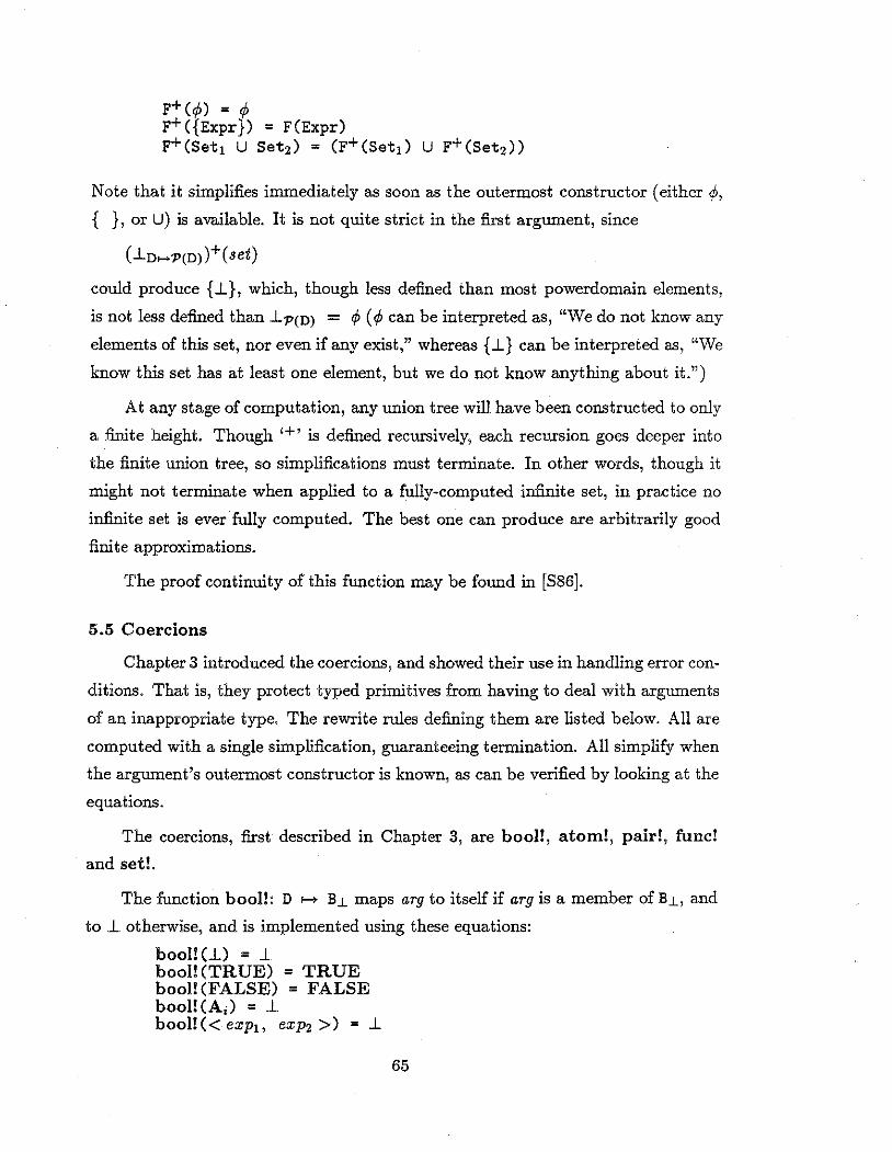
F+ (1/J) = ,P F+({Expr}) = F(Expr) F+ (Setl U Set2) = (F+ (Setl) U F+ (Set2))
Note that it simplifies immediately as soon as the outermost constructor (either ¢>,
{ }, or U) is available. It is not quite strict in the first argument, since
could produce {.l}, which, though less defined than most powerdomain elements,
is not less defined than .l'P(D) = ,P (¢>can be interpreted as, "We do not know any
elements of this set, nor even if any exist," whereas { .l} can be interpreted as, "We
know this set has at least one element, but we do not know anything about it.")
At any stage of computation, any union tree will have been constructed to only
a finite height. Though <+' is defined recursively, each recursion goes deeper into
the finite union tree, so simplifications must tenninate. In other words, though it
might not terminate when applied to a fully-computed infinite set, in practice no
infinite set is ever fully computed. The best one can produce are arbitrarily good
finite approximations.
The proof continuity of this function may be found in [586].
5.5 Coercions
Chapter 3 introduced the coercions, and showed their use in handling error con
ditions. That is, they protect typed primitives from having to deal with arguments
of an inappropriate type. The rewrite rules defining them are listed below. All are
computed with a single simplification, guaranteeing tennination. All simplify when
the argument's outermost constructor is known, as can be verified by looking at the
equations.
The coercions, first described in Chapter 3, are bool!, atom!, pair!, func!
and set!.
The function bool!: D >-+ B.1 maps arg to itself if arg is a member of B.1, and
to l.. otherwise, and is implemented using these equations:
boo!! (.l) = .l bool! (TRUE) = TRUE bool!(FALSE) = FALSE boo!! (A;) = .l boo!!(< exp1, exp2 >) = .l
65

bool! (.A ... ) = j_ bool! (r/>) = j_ bool!({ ... }) = j_ bool!( ... U ... ) = j_
The function atom!: D >-+ AJ. maps arg to itself if arg is a member of AJ., and
to j_ otherwise.
atom! (j_) = j_ atom! (TRUE) = j_ atom!(FALSE) = j_ atom!(A;) = A; atom!(< exp1, exP2 >) = j_ atom! (.A ... ) = j_ atom!(r/>) = j_ atom!({ ... }) = j_ atom!( ... U ... ) = j_
The function pair!: D >-+ DxD maps arg to itself if arg is a member of DxD,
and to j_DxD (that is, < j_, j_ >)otherwise.
pair! (j_) = < j_, j_ > pair! (TRUE) = < j_, j_ > pair!(FALSE) = < j_, j_ > pair! (A;) = < j_, j_ > pair!(< exp~, exJl2 >) = < exp1 , exJl2 > pair! (.A ... ) = < j_, j_ > pair! (r/>) = < j_, j_ > pair!({ ... }) = < j_, j_ > pair!( ... U ... ) = < j_, j_ >
The function func!: D >--+ [D>-+D] maps arg to itself if arg is a member of D>-+D
and to j_D,_.D (that is, .Ax. j_D, also written as !1) otherwise.
func! (j_) = n func! (TRUE) = n func!(FALSE) = n func! (A;) = !1 func!(< eXp!, €XJl2 >) = !1 func!(.A var. body) = .A var. bedy func!(r/>) = n func!({ ... }) = n func!( ... u ... ) = n
The function set!: D >--+ 'P(D) maps arg to itself if arg is a member of 'P(D)
and to j_:P(D) (that is, r/>) otherwise.
set! (j_) = r/> set! (TRUE) = r/> set! (FALSE) = r/>
66

set! (A;) = ¢> set!(< exp1 , exP2 >) = r/> set! (A ... ) = ¢> set! ( ¢>) = ¢> set! ( {element}) = {element} set! (set1 U set2) = set1 U set2
We can reduce sequences of coercions by noting that for two coercions c. and
c. ( Cb (arg)) = c. (arg) when c. and Cb are the same coercions. c. ( cb (arg)) = c. (.l) when c. and cb are different coercions.
For instance, we can simplify set!( set!( arg)) to set!( arg ), and set!( func!( arg)) to
¢>. The continuity of these functions was discussed at the end of Chapter 3.
5.6 Run-time Type-checking
PowerFuL is an untyped language. To allow the programmer to specify run
time type-checking, provide these primitive semantic functions over D 1-> BJ.: bool?,
atom?, pair?, func? and set?. We can determine an object's type by viewing
the outermost constructor, or in some cases, by the output type of the primitive
heading the argument (i.e. if the primitive never returns a result that is completely
undefined. For instance, the expression set?( set!( arg)) always denotes TRUE).
The equations defining bool? are:
boo I? (..L) = ..L bool?(TRUE) = TRUE bool?CFALSE) = TRUE bool?(A;) = FALSE bool?(< exp1. exP2 >) = FALSE bool?(A ... ) = FALSE bool?(r/>) = FALSE bool?({ ... }) = FALSE bool?(. .. u ... ) = FALSE. bool?(pair!(arg)) = FALSE. bool?(func!(arg)) = FALSE. bool?(set!(arg)) =FALSE. bool?(. .. + ... ) = FALSE.
In other words, bool? returns TRUE ifthe argument is a boolean, FALSE if the
argument is an atom, an ordered pair, a function or a set, and ..L if the object's type is
unknown. The primitive is computed with just one simplification, so termination is
guaranteed. When the outermost constructor of the object is known, simplification
can proceed.
67

The other type-checking primitives are similar, and have the same termination
and simplification properties. The equations for atom? are:
atom? (.l) = .l atom?(TRUE) = FALSE atom?(FALSE) = FALSE atom?(A;) = TRUE atom?(< expb exJ12 >) = FALSE atom?(>. ... ) = FALSE atom?(/fo) = FALSE atom?({ ... }) = FALSE atom?( ... u ... ) = FALSE. atom?(pair!(arg)) =FALSE. atom?(func!(arg)) =FALSE. atom?(set!(arg)) = FALSE. atom?( ... + ... ) = FALSE.
The equations for pair? are:
pair?(.l) = .l pair?(TRUE) = FALSE pair?(FALSE) = FALSE pair?(A;) = FALSE pair?(< exp1, exJ12 >) = TRUE pair?(>. ... ) = FALSE pair?(/fo) = FALSE pair?({ ... }) =FALSE pair?(. .. u ... ) = FALSE. pair?(pair!(arg)) = TRUE. pair?(func! (arg)) = FALSE. pair?(set!(arg)) =FALSE. pair?( ... + ... ) = FALSE.
The equations for func? are:
func? (.l) = .l func?(TRUE) = FALSE func?(FALSE) = FALSE func?(A;) = FALSE func?(< exp1, exJ12 >) = FALSE func? (>. •.• ) = TRUE func?(/fo) = FALSE func?({ ... }) = FALSE func?( ... u ... ) = FALSE. func?(pair!(arg)) = FALSE. func?(func!(arg)) = TRUE. func?(set!(arg)) =FALSE. func?(. .. + ... ) = FALSE.
The equations for set? are:
set? (.l) = .l set?(TRUE) = FALSE
68

set?(FALSE) = FALSE set?(A;) = FALSE set?(< exp1 , exP2 >) = FALSE set?(). ... ) = FALSE set?(<,D) = TRUE set?({ ... }) = TRUE set?(. .. U ... ) = TRUE. set? (pair! ( arg)) = FALSE. set? (func! ( arg)) = FALSE. set? (set! ( arg)) = TRUE. set?(. .. + ... ) = TRUE.
To prove continuity, note that, because these functions are monotonic, the
continuity requirement holds for all finite chains. For any infinite chain in D, the
least upper bound of the chain and every chain element (with the possible exception
of ..l.n are all contained within one of these subdomains: B1., A.L, D X D, D >-> D
and 'P(D). When applied to members of the same subdomain, each type-checking
always returns the same constant result, permitting continuity to be easily verified.
5. 7 Equality
We define first-order equality by saying that two first-order objects are equal
if and only if they are identical. First-order objects include atoms, booleans, and
nested ordered pairs whose leaves are atoms and booleans. We wish to define equal
ity over all first-order objects, not just atoms. There are several ways we could have
done this. We could have given the programmer access to the atomeq? primitive,
letting the user include a definition for equality within his program. Alternatively,
we could have defined equality construct via the denotation equations. However,
an important optimization technique developed in the next chapter requires that
equality be made a primitive. As a primitive strict in both arguments, there must be
a simplification available whenever the outermost constructor of either argument is
available. This motivates the following equations, broken into groups for discussion.
The first two equations simply indicate that the primitive is strict in both argu
ments.
equal?(..!., arg2) = ..!. equal? (arg1, ..!.) = ..!..
If we know anything at all about either argument, we know whether it is a member
of B (a boolean), A (an atom), DxD (an ordered pair), D>->D (a function) or 'P(D) (a
set). As soon as we know this about an argument (either by having computed the
69

outermost constructor, or by computing it to the form of a primitive application
headed by pair!, func!, set! or •+•), we can apply a simplification rule.
If B is known to be a boolean, then:
equal?(B, exp) = if bool?( exp) then if(B, bool!( exp ), not(bool!( exp ))) else FALSE fi
and by symmetry:
equal?( exp, B4 = If bool.(exp) then if(bool!(exp),B,not(B)) else FALSE fi.
If A is an atom, then
equal?(A, exp) = If atom?( exp) then atomeq?( A, atom!( exp)) else FALSE fi
and by symmetry
equal?(exp, A) = if atom?(exp) then atomeq?(atom!(exp),A) else FALSE fi
If F is a function, then
equal?(F, exp) -equal?( exp, F) -
if func?(exp) then .l else FALSE fi if func?(exp) then .l else FALSE fi
If Sis a set, then
equal?(S, exp) equal?( exp, S)
= if set?( exp) then .l else FALSE fi = if set?( exp) then .l else FALSE fi
If P is an ordered pair, then:
equal?(P, exp) = If not( pair?( exp )) then FALSE elseif not(equal?(left(P), left(pair!(exp)))) then FALSE else equal?(right(P), right(pair!( exp))) fi
and by symmetry:
equal?( exp, P) = If not(pair?( exp )) then FALSE elseif not( equal?(left(pair!( exp )), left( P) )) then FALSE else equal?( right( pair!( exp) ), right( P)) fi
Though the simplification rules for equal? are recursive, simplifications will
always terminate. The recursion only occurs when comparing two ordered pairs. At
any stage of computation, any ordered-pair tree will have been constructed to only a
70

finite height. Each recursion goes deeper into the finite union tree, so simplifications
must terminate. In other words, though it might not terminate when comparing
two identical fully-computed lists, in practice no infinite list is ever fully computed.
The best one can produce are arbitrarily good finite approximations.
Essentially, equal? is the least fixpoint of a recursive functional built usmg
the function composition of the function variable and continuous primitives, and is
therefore itself a continuous function [S86].
5.8 Summary
In this chapter, we have defined the primitives through equations which also
serve a rewrite rules. We have shown that each primitive does indeed simplify
upon availability of the outermost constructor of any argument in which it is strict.
We have also shown that the simplification stage of every computation step must
terminate.
With these definitions of the primitives, the definition of our language is com
plete. Because they satisfy the above properties, as required by the developments in
chapter 4, we have an operational semantics as well. The next chapter will improve
the interpretation procedure, and there these primitives play a central role.
71
6 OPTIMIZATIONS
This chapter improves the basic operational procedure described in the last
chapter. The problem being attacked is the inefficiency of relative set abstraction
when the set of terms acts as a generator. Rather than enumerating terms blindly,
we would like to treat the enumerated parameter as a logical variable, analogous to
the implementation of absolute set abstraction. This chapter explains why this is
proper to do, and provides a scheme for how to implement this optimization.
6.1 A voiding Generate-and-Test
In Section 2, we specified a Horn logic program using letrec (the feature
for creating recursive definitions), set abstraction, the conditional and the equality
primitive. Executing this program using PowerFuL's denotational equations as the
interpreter would be analogous to using Herbrand's method [Q82] to solve problems
in logic. Herbrand's "generate-and-test" approach is simple but inefficient.
The resolution method avoids blind generation of instantiations, preferring to
do as much work as possible on non-ground expressions. In logic programming, a
logical variable denotes an element from the set of terms (the Herbrand Universe).
In resolution, a logical variable becomes instantiated only to the extent necessary
to satisfy the inference rule's equality test. Partial instantiation narrows the set of
candidate bindings, without necessarily settling on a single choice. When performed
to ensure equality of non-ground terms, partial instantiation is called unification,
and the substitution implementing the partial instantiation is called a unifier.
In PowerFuL, to compute a relative set expression, we normally begin by com
puting the generator set. As an example, consider the following expression.

letrec
append be A 11 12. if null?(ll) then 12
else cons(car(ll), append(cdr(l1),12)) fi
in {X: X E terms, append(X, ['a,'b]) = ['c,'d,'a,'b]}
Whenever we isolate an expression denoting an element of the generator, in
this case a term, a copy of the relative set abstraction is created, with the generator
element expression replacing the enumeration parameter. In this case, the set terms
evaluates to a union tree, whose leaves are each a singleton set containing one term.
The set abstraction reduces to a union tree, each of whose leaves contains the value
denoted by
letrec
append be A 11 12. if null?(l1) then 12
else cons(car(ll), append(cdr(l1),12)) fi
in
{ term : append(term, ['a, 'b]) = ['c, 'd, 'a, 'bJ}
where term represents one element of the set of terms. It is clear that each such
instantiation can easily be computed. Where term satisfies the condition, the result
is a singleton set containing this term. For terms that do not satisfy the condition,
the result will be ¢. The complete result is union of all these subsets. We would
like to modify this procedure so that when terms is the generator set, we treat the
enumeration parameter as a logical variable, rather than blindly enumerating its
many simple objects. Similarly, an enumeration parameter generated by atoms, or
boola can be viewed as a partially-instantiated, or constrained, logical variable.
In Horn logic, each correct answer substitution provides ground bindings for the
goal's logical variables. Members of this set can be grouped into families. Within a
family, all answer substitutions share common aspects, with the remaining details
varying freely. The Herbrand derivation of one member of the family is almost iden
tical to the Her brand derivation for any other member. For each family of correct
answer substitutions, Herbrand's method would derive each member individually,
with an infinity of essentially similar derivations. Resolution, however, produces
most general computed answer substitutions, one per family. A general computed
answer substitution only partially instantiates a goal's logical variables, and does
73

so in such a way that for any ground completion of the general computed answer
substitution would result in a correct answer substitution. The derivation of the
general answer substitution resembles a parameterized Herbrand derivation.
Resolution performs modus ponens inferences on the non-ground clauses di
rectly, rather than first instantiating them. Logical variables become partially in
stantiated (via a most general unifier) only to the extent necessary to satisfy the
inference rule's equality requirement. Pure Horn logic ignores logical variable bind
ings which make the equality false. PowerFuL primitives are more complex, in that
we are interested in all possible logical variable bindings to produce all possible
results. However, some versions of Prolog [N85] add the inequality predicate as
well. Rather than actively generating bindings for logical variables, the inequality
primitive constrains future bindings.
In a sense, program execution is left unfinished. Though it is easy to extend a
most general answer substitution, to produce (ground) correct answer substitutions,
this is not done. Reporting results in the general form is more economical than
individually reporting each of the infinite ways in which each most general answer
can be extended.
6.2 Logical Variable Abstraction
To treat an enumeration parameter as a logical variable, we must recognize
that its generator is the set of first-order terms (or part of this set). An expression
of the form
(>..x.body)+ F[terms]
or equivalently
(>..x.body)+ set!(F[terms])
is rewritten at run-time to
term( x). body
to indicate that x is to be treated as a logical variable, rather than blindly enumer
ating its generator. We can look out for this situation by noting when the semantic
equation
t'([{expr : idE genrtr, qualifierlist}] p)
=(>..X. t'[{expr : qualifierlist}] p[Xjid])+(set!(t'[genrtr] p))
74
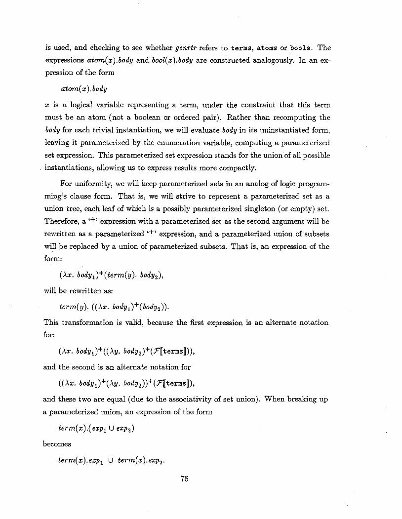
is used, and checking to see whether genrtr refers to terms, atoms or bools. The
expressions atom(x).body and bool(x).body are constructed analogously. In an ex
pression of the form
atom( x ). body
x is a logical variable representing a term, under the constraint that this term
must be an atom (not a boolean or ordered pair). Rather than recomputing the
body for each trivial instantiation, we will evaluate body in its uninstantiated form,
leaving it parameterized by the enumeration variable, computing a parameterized
set expression. This parameterized set expression stands for the union of all possible
instantiations, allowing us to express results more compactly.
For uniformity, we will keep parameterized sets in an analog of logic program
ming's clause form. That is, we will strive to represent a parameterized set as a
union tree, each leaf of which is a possibly parameterized singleton (or empty) set.
Therefore, a •+• expression with a parameterized set as the second argument will be
rewritten as a parameterized •+• expression, and a parameterized union of subsets
will be replaced by a union of parameterized subsets. That is, an expression of the
form:
will be rewritten as:
This transformation is valid, because the first expression is an alternate notation
for:
and the second is an alternate notation for
and these two are equal (due to the associativity of set union). When breaking up
a parameterized union, an expression of the form
becomes
term(x).exp 1 U term(x).exp2 •
75

A parameterized empty set, such as term( x ).¢>, can be simplified to ¢>, if desired.
One computes a parameterized set expression by expanding the occurrences of
the semantic function ( E, :F or 1J) in the parameterized body as specified by the
computation rule, and doing all possible primitive simplifications between expan
sion steps. In other words, one strives to compute the parameterized body just as
one would if each logical variable had been replaced by a ground term. Though
expansion of the semantic function is unaffected by the fact that some terms are
represented by logical variables, simplification of primitives becomes more difficult.
Simplification of primitives applied to logical variables is discussed in the next sec
tion.
6.3 Simplifying Primitives with Logical Variables
Suppose a parameterized body contains a subexpression headed by a primitive,
one of whose strict arguments is a logical variable. If the logical variable were
replaced by a term, we could simplify the primitive with the appropriate primitive
rewrite rule chosen according to the value of the term. But how do we choose which
rewrite rule to use, when the logical variable represents any of a whole range of
possible terms? For any such case, one of three techniques will permit simplification
of the primitive. Cases motivating each technique are listed below.
1) When the same rewrite rule would be chosen for any possible instantia
tion of the logical variable, Technique 1 allows us to simplify directly, without any
instantiation of the logical variable.
2) When the choice of rewrite rule depends upon whether a term represents a
boolean, an atom or an ordered pair, and the logical variable is unconstrained (i.e.
it could represent any of these), the second technique allows us to split into three
subsets, each of which handles one of the possibilities.
3) When two logical variables are being compared for equality, the third tech
nique splits the set into two subsets, one in which the equality is assumed to hold,
and the other in which an inequality constraint is generated.
We describe each case in the notation:
term( u ).( ... prim( u) . .. ),
where prim is some specific primitive. The ellipses indicate that the primitive subex-
76
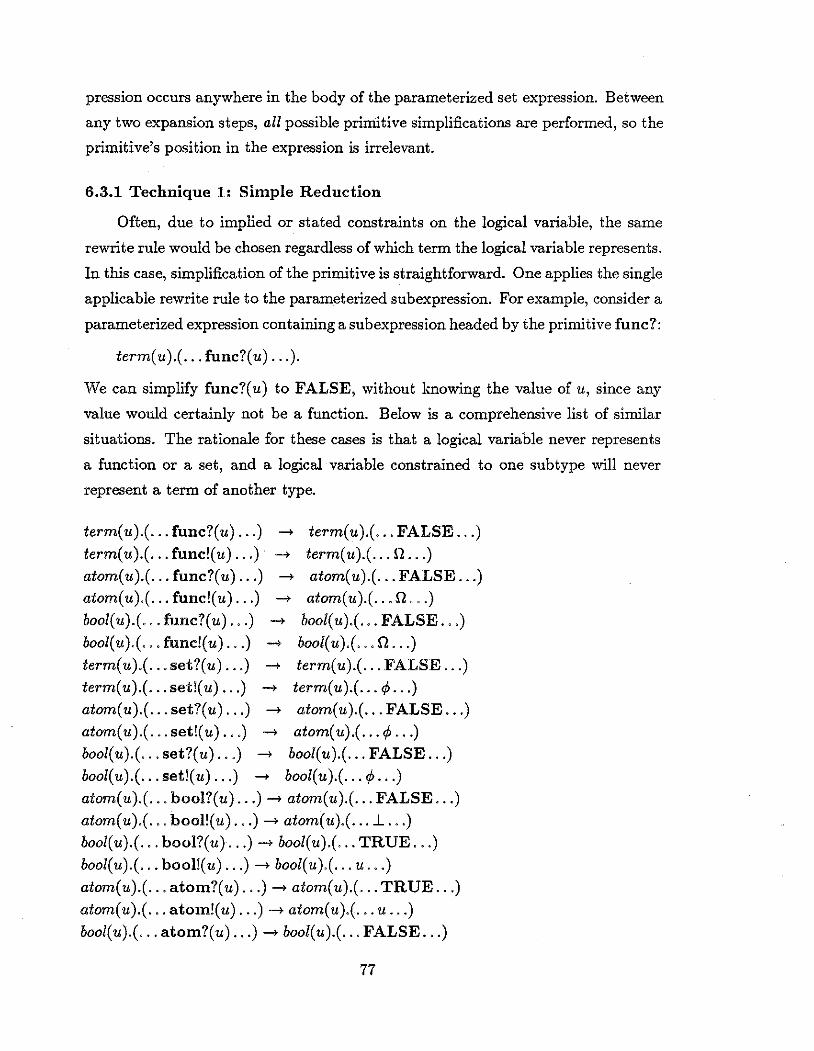
pression occurs anywhere in the body of the parameterized set expression. Between
any two expansion steps, all possible primitive simplifications are performed, so the
primitive's position in the expression is irrelevant.
6.3.1 Technique 1: Simple Reduction
Often, due to implied or stated constraints on the logical variable, the same
rewrite rule would be chosen regardless of which term the logical variable represents.
In this case, simplification of the primitive is straightforward. One applies the single
applicable rewrite rule to the parameterized subexpression. For example, consider a
parameterized expression containing a subexpression headed by the primitive func?:
term( u ).( ... func?( u) ... ).
We can simplify func?(u) to FALSE, without knowing the value of u, since any
value would certainly not be a function. Below is a comprehensive list of similar
situations. The rationale for these cases is that a logical variable never represents
a function or a set, and a logical variable constrained to one subtype will never
represent a term of another type.
term(u).( ... func?(u) ... ) --> term(u).(o. 0 FALSE ... ) term(u).( ... func!(u) .. o). --> term(u).( ... n ... ) atom(u).( ... func?(u) ... ) --+ atom(u).( ... FALSE ... ) atom(u).( ... func!(u) ... ) --> atom(u).( .. o!"!.oo) bool(u)o(o .. func?(u)oo•) --> bool(u).(.o.FALSE.oo) bool(u).(o 0 0 func!(u) ... ) -+ bool(u).(o 00 n. 0 o) term(u)o(o.oset?(u) ... ) -+ term(u).(o .. FALSE ... ) term( u).(o o. set!( u) .. . ) -+ term( u ).( ... <P •• • )
atom(u).( .. . set?(u) 0 •• ) -+ atom(u).( .. . FALSE ... )
atom( u )o(. 0. set!( u) .. . ) -> atom( u).( ... <P •• • )
bool(u).( ... set?(u) ... ) --+ bool(u).( ... FALSE ... ) bool(u).( .. . set!(u) ... ) -+ bool(u).( ... <,? ••• )
atom(u).( ... bool?(u) ... )--+ atom(u).( ... FALSE ... ) atom( u).(. o. bool!( u). 0 .) -+ atom( u)o( ... .l. o .) bool(u).( ... bool?(u) ... ) -+ bool(u)o(o .. TRUE ... )
bool( u).( ... boo!!( u) .. . ) --+ bool( u ).( ... u .. . ) atom(u).( ... atom?(u) .. . ) --+ atom(u).( . .. TRUE ... )
atom( u ).( ... atom!( u) ... ) -> atom( u ).( ... u ... ) bool(u).( ... atom?(u) ... ) -> bool(u).( ... FALSE ... )
77
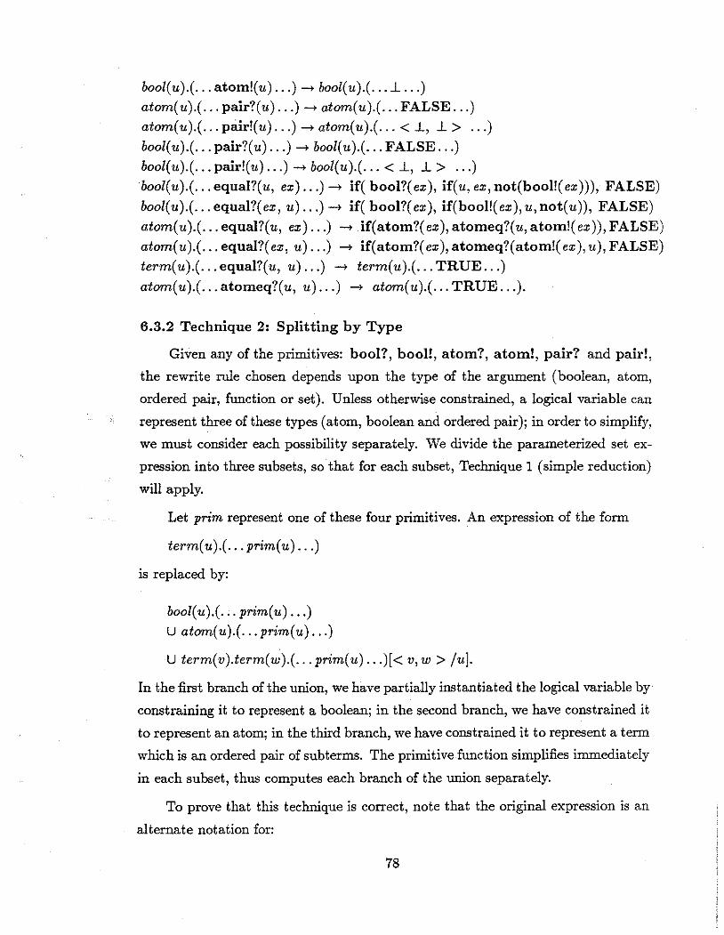
bool(u).( ... atom!(u) ... )--> bool(u).( ... .l ... )
atom(u).( ... pair?(u) . .. ) --> atom(u).( ... FALSE ... )
atom(u).( ... pair!(u) ... )->atom(u).( ... <.l, .l> ... )
bool(u).( ... pair?(u) .. . ) --> bool(u).( . .. FALSE ... )
bool(u).( ... pair!(u) ... ) --> bool(u).( ... < .l, .l > ... ) bool( u ).( ... equal?( u, ex) ... ) --> if( boo!?( ex), if( u, ex, not(bool!( ex))), FALSE)
bool(u).( ... equa!?(ex, u) ... )--> if( boo!?( ex), if(bool!(ex),u,not(u)), FALSE)
atom( u).( ... equal?(u, ex) ... ) --> if( atom?( ex), atomeq?(u, atom!( ex)), FALSE) atom( u).( ... equal?( ex, u) .. . ) --> if( atom?( ex), atomeq?(atom!( ex), u), FALSE)
term(u).( .. . equal?(u, u) .. . ) --> term(u).( ... TRUE ... )
atom(u).( ... atomeq?(u, u) ... ) --> atom(u).( ... TRUE ... ).
6.3.2 Technique 2: Splitting by Type
Given any of the primitives: boo!?, boo!!, atom?, atom!, pair? and pair!,
the rewrite rule chosen depends upon the type of the argument (boolean, atom,
ordered pair, function or set). Unless otherwise constrained, a logical variable can
represent three of these types (atom, boolean and ordered pair); in order to simplify,
we must consider each possibility separately. We divide the parameterized set ex
pression into three subsets, so that for each subset, Technique 1 (simple reduction)
will apply.
Let prim represent one of these four primitives. An expression of the form
term( u ).( ... prim( u) . .. )
is replaced by:
bool( u ).( ... prim( u) ... )
U atom(u).( ... prim(u) ... )
U term(v).term(w).( ... prim( u) .. . )(< v, w > /u].
In the first branch of the union, we have partially instantiated the logical variable by
constraining it to represent a boolean; in the second branch, we have constrained it
to represent an atom; in the third branch, we have constrained it to represent a term
which is an ordered pair of subterms. The primitive function simplifies immediately
in each subset, thus computes each branch of the union separately.
To prove that this technique is correct, note that the original expression is an
alternate notation for:
78

( ... prim(u) .. . )+(F[terms]).
Expanding F yields:
(F[bools]) U (F[atoms])
U (term(u).term(v). < u,v >).
Simplifying + by distributing ( ... prim( u) ... ) over the union yields:
( ... prim(u) ... )+(F[bools])
U ( ... prim(u) .. . )+(.r[atoms])
U ( •.. prim(u) .. .)+(term(v).term(w). < v,w >).
Putting this into the standard format for a parameterized set yields the replacement
expresswn.
This technique is analogous to narrowing in constructor-based term-rewriting
systems [R85], where, to permit further reduction of a non-ground term (a term
containing logical variables), one instantiates a variable in all possible ways which
would enable further reduction. This technique is also analogous to the use of most
general unifiers in Horn logic resolution. Unification prepares two clauses for modus
ponens by instantiating them no more than is necessary to satisfy the equality
requirement. One difference is that traditional Horn logic does not use negative
information. Horn logic only considers instantiations to make the equality true. In
PowerFuL, we are concerned with all possible outcomes. Some variations of Horn
logic do consider negative information through the use of a inequality predicate and
negative unifiers [N85] [K84]. We discuss primitives based on equality next.
6.3.3 Technique 3: Splitting on Equality
This section describes what to do when an argument of an equality primitive
(equal? or atomeq?) is a logical variable. Combined with the rewrite rules
for equality and the techniques given earlier, this technique implements syntactic
unification. Actually, a generalization of unification results, as negative bindings
(to make the equality false) are also considered.
Chapter 5 provided a comprehensive set of equal?'s rewrite rules. It simplifies
to a conditional expression whenever the type of either argument becomes known.
79

If the logical variable is constrained to one particular type, a simple reduction can
be performed, as was shown in a previous section.
If the lambda variable can represent more than one type, then, theoretically, one
could split according to type (divide into three cases, and then do simple reductions
for each case). In each case, the equality primitive would simplify to a conditional,
whose strictness demands that the type of the other argument be next ascertained.
However, a more efficient way is to delay the reduction of equality until the type of
the other argument (the one which is not a logical variable) is known, and simplify
according to itJ type. This way, preliminary computation of the other argument
needs be done only once, instead of three times.
When Both ArgumentJ are Logical VariableJ
If both arguments of the equality predicate are logical variables unconstrained
in type, then we mrut simplify. Consider an expression of the form:
term( u).( ... term( v ).( ... equal?( v, u) .. . ) ... )
This parameterized set expression contains somewhere in its body a primitive subex
pression comparing two unconstrained logical variables. Theoretically, one could
break this into an infinity of special cases, in each case u and v each being replaced
by an element of the set of terms. For some combinations the predicate equal?
would simplify to TRUE, and FALSE for other combinations. This could also
have been done with the primitives described earlier, but it is better to deal with
a few large subsets, than an infinity of individual cases. Splitting them into atoms,
booleans and ordered pairs does not help. We must recognize that the instantiations
fall into two cases: those for which the two terms are equal, and those for which
they are not. The subset handling the cases in which the two terms are equal can
be summarized by replacing all occurrences of v with occurrences of u:
term(u).( .. . term(v).( ... equal?(v, u) ... ) [v/u] ... ).
Since there are no more occurrences of v in the subexpression
term(v).( ... equal?(v, u) ... ) [v/u],
we can simplify this to
( .... ( ... TRUE ... ) [vfu]).
80

(In fact, this simplification can be performed whenever a body does not depend on
the enumerating variable. The special case of term( x). ¢> being replaced by ¢> was
given earlier.)
Inequality Constraints
We also need to summarize the cases when u and v are not equal. This could
be summarized by
term(u).( ... term(v).if not(equal?(v, u)) then ( ... FALSE ... ) else¢> ... ).
This summarizes the elements of the set for which which the two terms u and v are
not equal. Is there a way to compute this further, without trying individually all
possible combinations of unequal terms?
Lee Naish [N85] proposes for Prolog a inequality predicate, defined on terms.
His inequality predicate would fail when two terms are identical, succeed when two
terms cannot be unified, and delay when two terms are unifiable, but not identical.
In the last case, the other subgoals would be executed first, until the values of
logic variables have been instantiated enough to prove either the terms' equality or
their inequality. If all other subgoals succeed, without instantiating the variables
enough, Naish's Prolog gives an error message. This is not ideal behavior, since
unequal instantiations can certainly be computed. A better alternative woqld be
to make the inequality part of the solution, as a kind of negative unifier. Khabaza
describes a way in which this can be done [K84]. In essence, the inequality becomes
part of the general solution. Specific ground solutions can be generated from the
general solutions by instantiating logical variables in all possible ways subject to the
inequality constraint. Constraint logic programming [JL87] sets another precedent
for this approach. Computation of general non-ground solutions greatly improves
efficiency, and because replacing term variables by arbitrary ground terms is such a
trivial operation it matters little that the computation has terminates prematurely.
Requiring such term enumerations to satisfy a few inequalities adds little to the
complexity of the output, and makes it more compact.
To express such a constraint, we could write the above subset as:
term(u).( ... term(v)u =f v.( ... FALSE ... )).
81
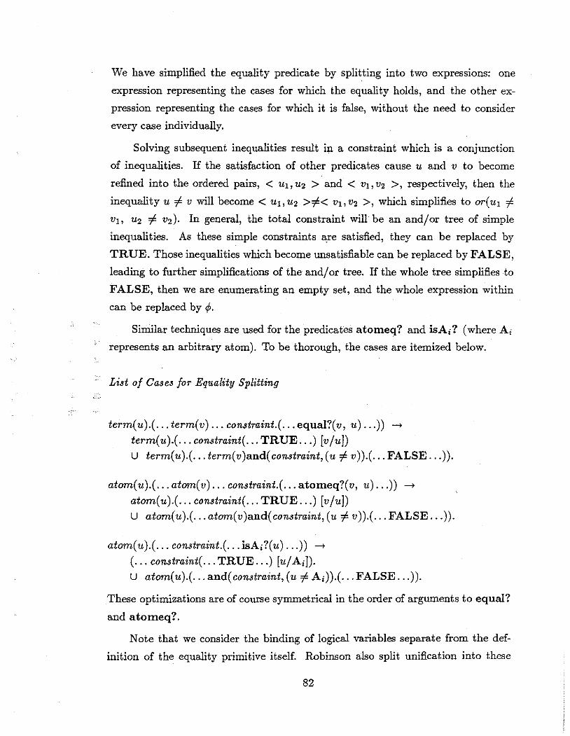
We have simplified the equality predicate by splitting into two expressions: one
expression representing the cases for which the equality holds, and the other ex
pression representing the cases for which it is false, without the need to consider
every case individually.
Solving subsequent inequalities result in a constraint which is a conjunction
of inequalities. If the satisfaction of other predicates cause u and v to become
refined into the ordered pairs, < u11 u2 > and < v11 v2 >, respectively, then the
inequality u =f v will become< u 1 ,u2 >=f< v11 v2 >,which simplifies to or(u1 =f vr, u2 =f v2). In general, the total constraint will be an and/or tree of simple
inequalities. As these simple constraints a,re satisfied, they can be replaced by
TRUE. Those inequalities which become unsatisfiable can be replaced by FALSE,
leading to further simplifications of the and/ or tree. If the whole tree simplifies to
FALSE, then we are enumerating an empty set, and the whole expression within
can be replaced by ¢.
Similar techniques are used for the predicates atomeq? and isA;? (where A;
represents an arbitrary atom). To be thorough, the cases are itemized below.
List of Cases for Equality Splitting
term(u).( ... term(v) ... constraint.( .. . equal?(v, u) . .. )) ->
term(u).( ... constraint( ... TRUE ... ) [vju]) U term(u).( ... term(v)and( constraint, ( u =f v)).( ... FALSE ... )).
atom( u).( ... atom( v) ... constraint.( ... atomeq?(v, u) . .. )) ->
atom(u).( ... constraint( ... TRUE ... ) [vju]) U atom(u).( ... atom(v)and(constraint,(u =f v)).( .. . FALSE ... )).
atom(u).( ... constraint.( .. . isA;?(u) ... )) ->
( ... constraint( ... TRUE ... ) [u/ A;]). U atom( u).( ... and( constraint, (u =fA;)).( ... FALSE ... )).
These optimizations are of course symmetrical in the order of argunrents to equal?
and atomeq?.
Note that we consider the binding of logical variables separate from the def
inition of the equality primitive itself. Robinson also split unification into these
82

components [BRS82]. We have generalized the approach to also consider negative
unification.
6.3.3 Discussion
We have already considered these primitives applied to logical variables: bool?,
t ? • ? f ? t? b I' t 1 • 1 f ' t' ·r t · A ? (" a om., patr., unc., se ., oo ., a om., patr .. , unc., se ., 1, no, Is i• 10r
each atom A;) and equal?. The primitives not discussed are: left, right, not, if,
t9-reduction and •+'.
According to the denotational equations, left and right are always applied
in conjunction with the coercion pair!. Since we have already considered logical
variables as arguments to pair!, we need no special mechanism for left and right.
The denotational equation producing function applications coerces the first
argument via the func! primitive. Since we have already considered logical variables
as arguments to func!, we need no special mechanism for t9-reduction, either.
Analogously, the coercion set! intercedes between •+' and its strict second
argument. Actually, since the second argument of •+, must be a set, one should
not expect to see a logical variable (which represents a term) in that position. We
have already discussed the case in which the second argument is a parameterized
set expression.
When a logical variable is an argument to not, or the first argument to if,
these arguments are protected by the coercion boo!!, so the logical variable must
already have been constrained to be a boolean. In that case, we simply split into two
subsets, one for which the logical variable is TRUE and one for which it is FALSE.
Though this involves a split, this is not really a special optimization technique. It
is the default procedure when bools is a relative set abstraction generator! The
only difference is that we delay the enumeration of bools until a boolean primitive
needs to know which one.
The only case not covered under any of these techniques is the case when a
logical variable represents a nonstrict argument of a primitive, e.g. if a logical
variable is the second or third argument of if. A semantic primitive of PowerFuL
will always simplify if it is given the outermost constructor of any strict argument. If
the primitive is not strict in that argument, however, the primitive will not simplify,
until something about a strict argument is known. So, consider
83

term(u).( .. . if((£[exp1 ] p),u, exp 3 ) • •• ).
Assuming the outermost constructor of exp1 is not available, the primitive if would
not yet simplify no matter which term might replace u. Therefore, the occurrence
of a logical variable in this position does not call for any special consideration.
6.4 Example
Suppose we wish to unify these two non-ground first-order terms: [A I B] and
[C I 'd] . i.e., to find replacements for logical variables A, B and C so that [A I B]
= [C I 'd]. It is clear that there are an infinite number of possible unifiers, each of
the form [A/D, B/'d, C/D] for some term D. In fact, this parameterized substitution
(parameterized by logical variable C) [A/D, B/' d, C/D] is the most general unifier.
It is a general unifier in that replacing C by any term will result in a unifier, and
most general in that any unifier is an instantiation of this form.
To calculate the set of unifiers, one might execute the Powerful program:
{ [AI[BIC]]: A,B,C E terms, [AIB]=[CI'd]}
That is, each unifier is represented by a list, whose elements are the respective
bindings for A, B and C. Removing some syntactic sugars, the denoted object is
defined as
E[{cons(A,cons(B,C)): A,B,C E terms,cons(A,B) = cons(C,' d)}] A.
Without the optimizations, this program would produce a set represented by
an infinite union tree with a leaf for each possible assignment of terms to A, B and
C. Where the assignment is a unifier, the leaf would be a singleton set containing
these bindings in a list. Where the assignment is not a unifier, the leaf would be
the empty set. The following derivation, however, uses the optimizations discussed
in this chapter, and succeeds in avoiding much redundant work. As we shall see, it
will construct a finite union tree, with a few leaves representing the empty set, and
a single leaf containing a parameterized singleton set. This parameterized singleton
set will represent the most general unifier [A/C, 'd/B]. Expanding the outermost
call, the above expression becomes
(AX. E[{cons(A, cons(B, c)) : B, C E terms, cons(A, B)= cons(C,' d)}] [X/A] )+set!(E[terms] A).
84
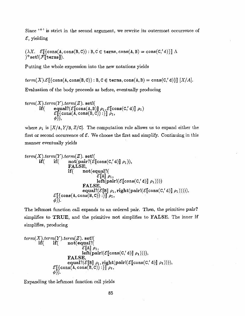
Since •+• is strict in the second argument, we rewrite its outermost occurrence of
£,yielding
(>.X. £[{ cons(A,cons(B, C)) : B, C E terms, cons(A, B)= cons(C,1 d)}] A )+set!(F[terms]).
Putting the whole expression into the new notations yields
term( X).£[{ cons( A, cons(B, c)) : B, C E terms, cons( A, B) = cons(C,' d)}] [X/ A].
Evaluation of the body proceeds as before, eventually producing
term( X).term(Y).term(Z). set!( if( efual?(E[cons(A,B)] p1 ,£[cons(C,' d)] p1 )
£ {cons( A, cons(B, C)) :} ] PI, q, ),
where PI is [XjA,YjB,Z/C]. The computation rule allows us to expand either the
first or second occurrence of£. We choose the first and simplify. Continuing in this
manner eventually yields
term( X).term(Y).term(Z). set!( if( if( not(pair?(E[cons(C,' d)] pi)),
FALSE, if( not( equal?(
£[A] Pl• left(pair!(E[cons(C,' d)] PI))))
FALSE, equal?(E[B] PI, right(pair!(E[cons(C,' d)] PI))))),
t'[ {cons( A, cons(B, C)) :} ] PI, q, )).
The leftmost function call expands to an ordered pair. Then, the primitive pair?
simplifies to TRUE, and the primitive not simplifies to FALSE. The inner if
simplifies, producing
term(X).term(Y).term(Z). set!( if( if( not( equal?(
£[A] P1, left(pair!(E[cons(C,' d)] PI)))),
FALSE, equal?(E[B] p1,right(pair!(£[cons(C,' d)] PI)))),
£[ {cons( A, cons(B, c)) : }H PI, ¢> )).
Expanding the leftmost function call yields
85
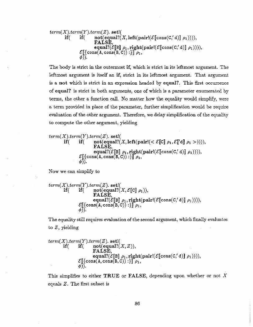
term(X).term(Y).term(Z). set!( if( if( not(equal?(X,left(pair!(£[cons(C,' d)] PI)))),
FALSE, equal?(£[B] PI>right(pair!(£[cons(C,' d)] PI)))),
£[{cons(A,cons(B,C)) :}] PI, 1/>J).
The body is strict in the outermost if, which is strict in its leftmost argument. The
leftmost argument is itself an if, strict in its leftmost argument. That argument
is a not which is strict in an expression headed by equal?. This first occurrence
of equal? is strict in both arguments, one of which is a parameter enumerated by
terms, the other a function call. No matter how the equality would simplify, were
a term provided in place of the parameter, further simplification would be require
evaluation of the other argument. Therefore, we delay simplification of the equality
to compute the other argument, yielding
term(X).term(Y).term(Z). set!( if( if( not( equal?( X, left( pair!(< £[c] PI,£[' d] PI >))) ),
FALSE, . equal?(£[B] PI, right(pair!( £[cons(C,' d)] PI)))),
£[ {cons( A, cons(B, C)) :} ] PI, 4> )).
Now we can simplify to
term(X).term(Y).term(Z). set!( if( if( not( equal?( X, £[c] PI)),
FALSE, equal?(£[B] PI, right(pair!(£[cons(C,' d)] pi)))),
£[{cons( A, cons(B, c)) : }] PI, 4> J).
The equality still requires evaluation of the second argument, which finally evaluates
to Z, yielding
term(X).term(Y).term(Z). set!( if( if( not( equal?(X, Z)),
FALSE, equal?(£[B] PI,right(pair!(£[cons(C,' d)] PI)))),
£[ {cons( A, cons(B, C)) :} ] Pb 4>)).
This simplifies to either TRUE or FALSE, depending upon whether or not X
equals Z. The first subset is
86
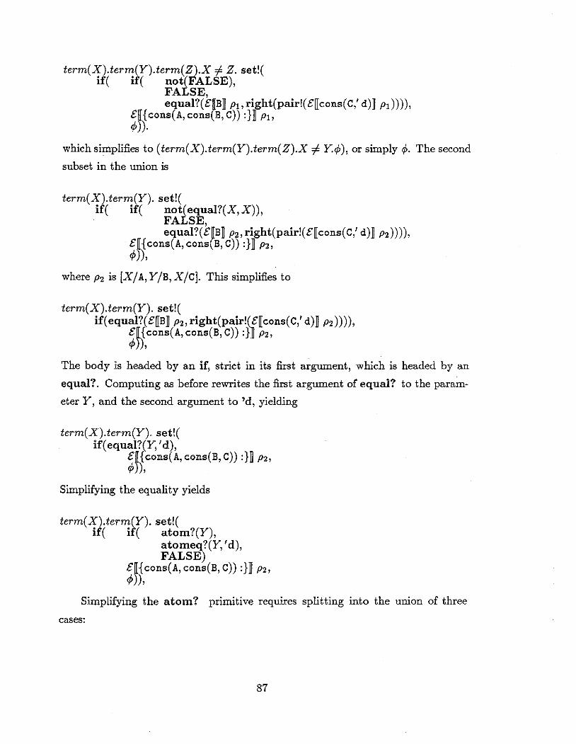
term(X).term(Y).term(Z).X # Z. set!( if( if( not(FALSE),
FALSE, equal?(£[B] P1,right(pair!(£[cons(C,1 d)] p1)))),
£[ {cons( A, cons(B, C)) :}] P1, <I>)).
which simplifies to (term(X).term(Y).term(Z).X # Y.</>), or simply¢>. The second
subset in the union is
term(X).term(Y). set!( if( if( not(equal?(X,X)),
FALSE, equal?(£[B] p2,right(pair!(£[cons(C,' d)] p2)))),
£[ {cons( A, cons(B, c)) :} ] P2, <I>)),
where p2 is [X/ A, Y /B, X/C]. This simplifies to
term(X).term(Y). set!( if( equal?( £[B] P2, right(pair!( £[cons(C,' d)] P2)))),
£[ {cons( A, cons(B, C)) :}] P2, <I>)),
The body is headed by an if, strict in its first argument, which is headed by an
equal?. Computing as before rewrites the first argument of equal? to the param
eter Y, and the second argument to 'd, yielding
term(X).term(Y). set!( if( equal?(Y, 1 d),
£[{cons( A, cons(B, C)) :}D P2, <I>)),
Simplifying the equality yields
term(X).term(Y). set!( if( if( atom?(Y),
atomeq?(Y, 'd), FALSE)
E[ {cons( A, cons(B, C)) :}] P2, </>)),
Simplifying the atom? primitive requires splitting into the union of three
cases:
87

term(X).bool(Y). set!( if( 1f( FALSE,
atomeg._?(Y, 'd), FALSE)
f[ {cons( A, cons(B, C)) : }D P2, <P) ),
term(X).atom(Y). set!( if( if( TRUE,
and
atomeq?(Y, 'd), FALSE)
f[ {cons( A, cons(B, C)) : }D P2, <P J),
term(X).term(Yi).term(Y2 ) set!( if( if( atom?(< Yi, Y2 > ),
atomeq?( < Yi, Y2 >, 1 d), FALSE)
f[{cons(A,cons(B,C)) :}] Pa, </1)),
where p3 is [X/ A,< Yb Y2 > /B, X/C]. The first and third subsets simplify to ¢1,
but the second simplifies to
term(X).atom(Y). set!( if( is' d(Y),
f[{cons(A,cons(B,C)) :}D P2, <P )).
Simplifying is'd? requires splitting Y into two cases:
term(X).atom(Y).Y =J 'd. set!( ¢1)).
which simplifies to </1, and
term(X). set!(f[{cons(A,cons(B,C)) :}] [X/A,'d/B,X/C]).
This latter clearly evaluates to
term(X). ({<X, < 'd,X >}).
Theoretically, we should still compute this expression as the union of all possible
instantiations, each instantiation replacing the logical variable X by a first-order
term (or approximate the result by doing some of these instantiations). For practical
88

purposes, such instantiation is trivial, so computation would terminate here. The
final result of this calculation is therefore a finite union tree, with </> for the first few
leaves (for the branches which split off earlier) and the last leaf being the above.
6.5 Correctness Observations
Soundness: Ift; is a partially computed parameterized set expression, and t;[fl/£]
is an approximation produced by setting all unevaluated function calls ('D, £or :F)
to ..l, then for every instantiation !7 replacing logical variables with terms satisfying
the constraints, t;[fl/ £] !7 approximates a subset of U{ t;[fl/ £]}.
Proof: The theorem is true because of the meaning of a parameterized expression
(in terms of •+•), and the fact that all steps in a parameterized derivation replace
expressions by equals. End of Proof
Completeness: Any element of a set which can be computed by a non-optimized
derivation can be computed as an instantiation of a parameterized derivation.
Proof: This theorem is true because when dividing a parameterized expression
into cases (for the purpose of simplifying a primitive), every possible instantiation
of logical variables which satisfies the constraints is a possible instantiation of one of
the subcases. No possible instantiation is ever lost. Furthermore, any computation
which can be performed after replacement of the enumeration variable by a term
can be performed on the parameterized body. End of Proof
6.6 Summary -
A type 1 simplification (simple reduction) does not require splitting; a type
2 simplification (splitting by type) requires a three-way split; type 3 simplifica
tions (splitting on equality) requires a two-way split. When performing primitive
simplifications, it is efficient to do first those simplifications which do not split the
computation into subcases, then those which split into two subcases and save for last
those requiring a three-way split. These optimizations avoid blind enumeration of
the sets terms, atoms and bools when used as relative set abstraction generators.
Instead, the enumeration parameter becomes a logical variable. An enumeration
variable from the set atoms is treated as a logical variable carrying the constraint
that it can be bound only to an atom. Enumeration variables from the set bools are
handled analogously. Inequality constraints relating two logical variables are also
89
used. The logical variables are instantiated only to the extent needed to simplify
the body. Wherever a logical variable is the argument of a primitive function, and
the primitive function needs more information about its argument to execute, the
generating set is divided into a few subsets, thereby dividing the whole expression
into subsets. In each subset, the range of the logical variable is narrowed enough
that the primitive has enough information to execute. Computing with logical vari
ables and constraints gives the set abstraction facility "resolution-like" efficiency.
Treating an enumeration parameter as a logical variable is practical because the
generating set terms is so simple in structure.
The optimizations described in this chapter modify the simple (though inef
ficient) operational semantics derived from the denotational equations in Chapter
4. Even with these optimizations, the result is far from a production-level imple
mentation! The purpose was rather to explain the role of the logical variable in
functional programming with set abstraction. The syntax and denotational seman
tics of PowerFuL made no reference to logical variables. The logical variable is
merely an operational concept to improve the execution efficiency when terms is
used as a generator. More complicated sets are also permitted as generators (e.g.
such as sets of functions, sets of sets, etc.), and in these cases, the default mechanism
(generate, instantiate, and continue) is used.
90

7 CONCLUSIONS
During the past decade, proponents of declarative programming languages have
discussed the possibility of combining of functional and logic programming styles
within one declarative language. Many proposals have been based on equational
logic, reasoning that equations could be used to define both functions and relations.
A weakness of this approach is the difficulty of maintaining functions (and other
higher-order constructions) as first-class objects. Testing higher-order objects for
equality is very difficult, and is not always computable, so a higher-order exten
sion will either relinquish referential transparency (through the use of an efficient
but unreliable higher-order equality test), or will require a very difficult and per
haps impractical, operational primitives such as higher-order unification, general
theorem-proving and unrestricted narrowing. Traditional functional programming,
in contrast, does not require tests of equality when passing arguments to proce
dures, and so avoids this problem. Since our approach is based on ordinary func
tional programming, incorporation of higher-order programming proved to be no
problem. Our approach supports both functions and sets as first-class higher-order
constructs. The underlying theses of our approach are:
1) Functional programming with relative set abstraction subsumes the expres
siveness of logic programming.
2) The resulting language does not require higher-order unification to maintain
first-class higher-order objects.
3) The use of logical variables is most properly viewed as an implementation
tool rather than as part of the language definition.
7.1 Results and Contributions
The principal results of this dissertation are:

(i) Relative set abstraction can combine lazy higher-order functional program
ming not only with first-order Horn logic, but also with a useful subset of higher
order Horn logic. Sets, as well as functions, can be treated as first-class objects.
(ii) Angelic powerdomains provide the semantic foundation for relative set ab
straction.
(iii) The computation rule appropriate for this language is a modified parallel
outermost, rather than the more familiar left-most rule.
(iv) Optimizations incorporating ideas from narrowing and resolution greatly
improve the efficiency of the interpreter, while maintaining correctness.
We are not the first to advocate set abstraction as a means of incorporating
Horn logic capability into higher-order functional programming. However, we do
believe this design is the first to be rigorously described via denotational seman
tics, mapping the syntax onto computable semantic primitives. The brevity and
simplicity of the denotational description attests to the elegance and integrity of
the design. To consider set-valued functions and sets as objects, we had to incor
porate angelic powerdomains into the complete semantic domain (each object in a
powerdomain represents a set of elements from some simpler domain). Our use of
powerdomains is novel in that we make the set an explicit data type, rather than
the implicit result of a non-deterministic control structure.
Horn logic programming can be described by either the fixed-point semantics
(closely related to Horn logic's model-theoretic semantics) or by its operational
semantics (SLD resolution). Soundness and completeness proofs attest the equiv
alence of these two descriptions. We feel that this result is an important feature
of Horn logic programming, and that our language should have a similar property.
Extending Vuillemin's theory of correct implementation of recursion, and apply
ing the resulting technique to the denotational equations themselves, we derived
an operational semantics equivalent to the denotational description. We think this
novel technique may be an important addition to the methodology of functional
programming, independent of the set abstraction problem.
To derive equivalent operational semantics by this technique, the denotational
semantics must handle most recursion explicitly, ensuring that primitives will al
ways terminate. Primitives must be rigorously defined via rewrite rules, rewriting
92

whenever the outermost constructor of any strict argument is available. Though
these restrictions make writing the denotational semantics more difficult, they en
sure the rigor of the definition. In extending Vuillemin's theory, we propose a new
computation rule which is a compromise between the parallel-outermost and the
leftmost computation rules. Like the leftmost rule, it permits evaluation to concen
trate in a primitive's strict arguments, but provides for parallel evaluation where
necessary due to the presence of non-flat domains.
Of special interest for logic programming is the set of terms, objects for which
identity is synonymous with equality. We showed that, when the set of terms is
used as a generating set in a relative set abstraction, the enumeration parameter
can be computed as a logical variable, instead of using the default blind generate
and-test procedure which would otherwise result. In the general case, however, the
enumeration parameters are instantiated by the various generator set elements as
these elements are computed. Thus, generators need not be arbitrarily restricted to
contain only first-order types.
Incorporating logical variables into the operational procedure complicates the
simplification of semantic primitives. That is, simplification sometimes requires
knowing more about a primitive's argument than that it is a term. It may depend
upon whether the logical variable represents an atom, a boolean or an ordered pair.
In such a case, we split the set into three subsets, one for each assumption. In each
subset, the primitive can simplify. A similar splitting procedure is used for handling
equality /inequality primitives.
7.2 Further Work
Several areas of additional research seem apparent:
1) Our decision to derive the operational semantics from the denotational equa
tions was motivated by a desire to ensure that the operational semantics remained
true to the denotational definition, and not by a conviction that this kind of inter
pretation would be most efficient. Practical software to implement this language
should make use of a more efficient strategy. The optimizations described in chap
ter 6 do not address the inefficiencies of interpreting from semantic equations in
general; rather, they solve a separate problem specific to set abstraction, i.e. the
desire to use logical variables in computing set abstractions generated by the set of
93

first-order terms. A challenging problem would be to describe this optimization in
terms of a more conventional operational semantics. In this dissertation we strove
to unify the declarative aspects of functional and logic programming; combining the
efficient implementation strategies developed for these kinds of languages (W83b]
(P87] is yet another topic.
2) Possible inefficiency aside, we feel that generating operational semantics from
denotational equations is an interesting idea, giving much insight as to the relation
between denotation and computation. We would like to study further the semantics
of denotational semantics as a programming language. From our experience in this
research, we feel that next time it might be better to define the semantics of the
language in terms of typed lambda calculus. This should permit greater rigor in
proving the relationship between operational and denotational semantics.
3) We would like to supplement PowerFuL with a polymorphic type system like
those provided for many other modern functional languages. This would lead to
many types of constructors. The most interesting aspect would be its effect on the
optimizations providing for logical variables. Would it increase the complexity of
computing with logical variables? Our feeling is that it might make the interpreter
more complex, but ought not to hurt efficiency.
4) Computation of infinite sets requires closer interaction between user and
interpreter. This places additional demands on the language environment, so new
programming enVironments may also need to be developed.
94

[A82]
[A83]
[AS85]
[AW82]
[BL86]
[BRS82]
[CK81]
[CM81]
[D74]
[D83]
[DP85]
References
S. Abramsky, "On Semantic Foundations for Applicative Multipro
gramming," In LNCS 154: Proc. 1Oth ICALP, Springer, Berlin, 1982,
pp. 1-14.
S. Abramsky, "Experiments, Powerdomains, and Fully Abstract Mod
els for Applicative Multiprogramming," In LNCS 158: Foundations of
Computation Theory, Springer, Berlin, 1983, pp. 1-13.
H. Abelson, G. Sussman, Structure and Interpretation of Computer
Programs, MIT Press, Cambridge, 1985.
E. A. Ashcroft and W. W. Wadge, "Prescription for Semantics," A CM
Transactions on Programming Languages and Systems, Vol. 4, No. 2,
April 1982, pp. 283-294.
M. Bellia and G. Levi, "The Relation between Logic and Functional
Languages: A Survey," In J. of Logic Programming, vol. 3, pp.217-236,
1986.
K. Berkling, J. A. Robinson and E. E.G. Siebert, "A Proposal for a
Fifth Generation Logic and Functional Programming System, Based
on Highly Parallel Reduction Machine Architecture," Syracuse Univ.,
Nov. 1982.
J. S. Conery and D. F. Kibler, "Parallel Implementation of Logic Pro
grams." In Conf Functional Prog. Lang. and Comp. Arch., ACM,
1981, pp. 163-170.
W. F. Clocksin and C. S. Mellish, Programming in Prolog, Springer
Verlag, New York, 1981.
J. B. Dennis, "First Version of a Data Flow Procedure Language." In
Lecture Notes in Comp. Sci., Ed. G. Goos and J. Hartmanis, Springer
Verlag, New York, 1974, pp. 362-376.
J. Darlington, "Unification of Functional and Logic Programming,"
internal report, Imperial College, 1983.
N. Dershowitz and D. A. Plaisted, "Applicative Programming cum
Logic Programming," In 1985 Symp. on Logic Programming, Boston,
95

[DFP86]
[DG89]
[F84]
[F84b]
[G88]
(GJ89]
[GM84]
[H80a]
[H80b]
[JLM84]
(JL87]
MA, July 1985, pp. 54-66.
J. Darlington, A.J. Field, and H. Pull, "Unification of Functional and
Logic Languages," In DeGroot and Lindstrom (eds.), Logic Program
mmg, Relations, Functions and Equations, pp. 37-70, Prentice-Hall,
1986.
J. Darlington, Y. Guo, "Narrowing and Unification in Functional Pro
gramming - An Evaluation Mechanism for Absolute Set Abstrac
tion," In 3rd International Conference, Rewriting Techniques and Ap
plications, Chapel Hill, NC, April 1989, pp. 92-108.
L. Fribourg, "Oriented Equational Clauses as a Programming Lan
guage." J. Logic Frog. 2 (1984) pp. 165-177.
L. Fribourg, "A Narrowing Procedure for Theories with Constructors."
In Proceedings of the 7th International Conference on Automated De
duction, LNCS 170 (1984) pp. 259c301.
J. Goguen, "Higher Order Functions Considered Unnecessary for
Higher Order Programming", SRI Project No. 1243, SRI International,
1988, 29 pages.
G. Gupta and B. Jayaraman, "Compilied And-Or Parallelism on
Shared-memory Multiprocessors," to appear in North American Con
ference on Logic Programming, Oct. 1989, 20 pp.
J. A. Goguen and J. Meseguer, "Equality, Types, Modules, and
(Why Not?) Generics for Logic Programming," J. Logic Frog., Vol.
2, pp. 179-210, 1984.
G. Huet, "Confluent Reductions: abstract properties and applications
to term rewriting systems," J. A CM, 27, 1980, pp. 797-821.
P. Henderson, Functional Programming Application and Implementa
tion, Prentice-Hall International, 1980.
J. Jaffar, J.-L. Lassez, M. J. Maher, "A Theory of Complete Logic
Programs with Equality," In J. Logic Frog., Vol. 1, pp. 211-223, 1984.
J. Jaffar, J.-1. Lassez, "Constraint Logic Programming," In 14th ACM
POPL, pp. 111-119, Munich, 1987.
96

[JS86] B. Jayaraman and F.S.K. Silbermann, "Equations, Sets, and Reduc
tion Semantics for Functional and Logic Programming," In 1986 ACM
Conf on LISP and Functional Programming, Boston, MA, Aug. 1986,
pp. 320-331.
(K79] R. A. Kowalski, "Algorithm = Logic + Control," In Communications
of the A CM, July 1979, pp. 424-435.
[K83] W. A. Kornfeld, "Equality for PROLOG," In Proceedings of the 8th
IJCAI, 1983, pp. 514-519.
[K84] T. Khabaza, "Negation as Failure and Parallelism." In Internatl. Symp.
Logic Programming, IEEE, Atlantic City 1984, pp. 70-75.
[L84] J. Lloyd, Foundations of Logic Programming, Springer-Verlag, New
York, 1984.
[L85]
[LWH88]
[M65]
[M74]
[M80]
[M82]
G. Lindstrom, "Functional Programming and the Logical Variable,"
In 12th ACM Symp. on Prine. of Prog. Langs., New Orleans, LA, Jan.
1985, pp. 266-280.
E. Lusk, D.H.D. Warren, S. Haridi et. a!. "The Aurora Or-Prolog Sys
tem", In Proceedings of the International Conference on Fifth Gener
ation Computer Systems, Tokyo, 1988, pp. 819-830.
J. McCarthy, eta!, LISP 1.5 Programmer's Manual, MIT Press, Cam
bridge, Mass., 1965.
Z. Manna, Mathematical Theory of Computation, McGraw-Hill Inc.,
New York, 1974.
G. A. Mag6, "A Cellular Computer Architecture for Functional Pro
gramming." Digest of Papers, IEEE Computer Society COMPCON
(Spring 1980) pp. 179-187 .
. T. Moto-oka (ed.) Fifth Generation Computer Systems, Proc. of Inti.
Conf. on Fifth Generation Systems, Japan Information Processing De
velopment Center (North-Holland), 1982.
[M83] B. J. MacLennan, Principles of Programming Languages, Holt, Rine
hart and Winston, New York, 1983.
[MMW84] Y. Malachi, Z. Manna, and R. Waldinger, "TABLOG: The Deductive-
97
[MN86]
[N85]
[P81]
[P82]
Tableau Programming Language," In ACM Symp. on LISP and Func
tional Programming, Austin, TX, Aug. 1984, pp. 323-330.
D. Miller and G. Nadathur, "Higher-Order Logic Programming," In
Third International Conference on Logic Programming, London, July
1986, 448-462.
L. Naish, "Negation and Control in Prolog," Doctoral Dissertation,
University of Melbourne, 1985.
F. G. Pagan, Formal Specification of Programming Languages, Prentice
Hall, Inc., Englewood Cliffs, New Jersey, 1981.
G. Plotkin, "The Category of Complete Partial Orders: a Tool for Mak
ing Meanings," Postgraduate lecture notes, Computer Science Dept.,
Univ. of Edinburgh, Edinburgh, 1982.
[P87] S.L. Peyton Jones, The Implementation of Functional Programming
[Q82]
[R85]
[R86]
Languages, Prentice-Hall, 1087.
W. Quine, Methods of Logic, Harvard University Press, Cambridge,
1982.
U. S. Reddy, "Narrowing as the Operational Semantics of Functional
Languages," In 1985 Symp. on Logic Programming, Boston, MA, July
1985, pp. 138-151.
J. A. Robinson, "The Future of Logic Programming," Symposium on
Logic in Computer Science, Ireland, 1986.
[S77] J. E. Stay, "Denotational Semantics: The Scott-Strachey Approach to
Programming Language Theory," MIT Press, Cambridge, Mass., 1977.
[S86J D. A. Schmidt, "Denotational Semantics: A Methodology for Language
Development," Allyn and Bacon, Inc., Newton, Mass., 1986.
[S89]
[SJS9]
D. A. Schmidt, personal communication, April1989.
F.S.K. Silbermann and B. Jayaraman, "Set Abstraction in Functional
and Logic Programming," To appear in 1989 ACM Conf on Func
tional Programming and Computer Architecture, London, UK, Sept.
1989.
98

[SP85]
[T81]
[V74]
[VK76]
[W83a]
[W83b]
(YS86]
G. Smolka and P. Panangaden, "A Higher-order Language with Uni
fication and Multiple Results," Tech. Report TR 85-685, Cornell Uni
versity, May 1985.
D. A. Turner, "The semantic elegance of applicative languages," In
ACM Symp. on Func. Prog. and Comp. Arch., New Hampshire, Octo
ber, 1981, pp. 85-92.
J. Vuillemin, "Correct and Optimal Implementations of Recursion in
a Simple Programming Language," Journal of Computer and System
Sciences 9, 197 4, 332-354.
M. H. van Emden and R. A. Kowalski, "The Semantics of Predicate
Logic as a Programming Language," J. ACM23, No.4 (1976) pp. 733-
743.
D. H. D. Warren, "Higher-order Extensions of Prolog: Are they
needed?" Machine Intelligence 10, 1982, 441-454.
D. H. D. Warren, "An Abstract Instruction Set for Prolog'', Tech. Note
309, SRI International, 1983, 28 pages.
J-H. You and P. A. Subrahrnanyam, "Equational Logic Programming:
an Extension to Equational Programming," In 13th ACM Symp. on
Prine. of Prog. Langs., St. Petersburg, FL, 1986, pp. 209-218.
99