a description and assessment of the new global foam - gmdd

GMDD6, 6219–6278, 2013

A description andassessment of thenew Global FOAM

system

E. W. Blockley et al.

Title Page

Abstract Introduction

Conclusions References

Tables Figures

J I

J I

Back Close

Full Screen / Esc

Printer-friendly Version

Interactive Discussion

Discussion

Paper

|D

iscussionP

aper|

Discussion

Paper

|D

iscussionP

aper|

Geosci. Model Dev. Discuss., 6, 6219–6278, 2013www.geosci-model-dev-discuss.net/6/6219/2013/doi:10.5194/gmdd-6-6219-2013© Author(s) 2013. CC Attribution 3.0 License.

Open A

ccess

GeoscientificModel Development

Discussions

This discussion paper is/has been under review for the journal Geoscientific ModelDevelopment (GMD). Please refer to the corresponding final paper in GMD if available.

Recent development of the Met Officeoperational ocean forecasting system:an overview and assessment of the newGlobal FOAM forecastsE. W. Blockley, M. J. Martin, A. J. McLaren, A. G. Ryan, J. Waters, D. J. Lea,I. Mirouze, K. A. Peterson, A. Sellar, and D. Storkey

Met Office, FitzRoy Road, Exeter, EX13PB, UK

Received: 1 November 2013 – Accepted: 19 November 2013 – Published: 29 November 2013

Correspondence to: E. W. Blockley ([email protected])

Published by Copernicus Publications on behalf of the European Geosciences Union.

6219

http://www.geosci-model-dev-discuss.net

http://www.geosci-model-dev-discuss.net/6/6219/2013/gmdd-6-6219-2013-print.pdf

http://www.geosci-model-dev-discuss.net/6/6219/2013/gmdd-6-6219-2013-discussion.html

http://creativecommons.org/licenses/by/3.0/

GMDD6, 6219–6278, 2013


system


Title Page



Tables Figures

J I

J I

Back Close

Full Screen / Esc



Discussion

Paper

|D

iscussionP

aper|

Discussion

Paper

|D

iscussionP

aper|

Abstract

The Forecast Ocean Assimilation Model (FOAM) is an operational ocean analysis andforecast system run daily at the Met Office. FOAM provides modelling capability in bothdeep ocean and coastal shelf seas regimes using the NEMO ocean model as its dy-namical core. The FOAM Deep Ocean suite produces analyses and 7 day forecasts of5

ocean tracers, currents and sea ice for the global ocean at 1/4◦ resolution and at 1/12◦

resolution in the North Atlantic, Indian Ocean and Mediterranean Sea. Satellite and in-situ observations of temperature, salinity, sea level anomaly and sea ice concentrationare assimilated by FOAM each day over a 48 h observation window. The FOAM DeepOcean configurations have recently undergone a major upgrade which has involved:10

the implementation of a new variational, first guess at appropriate time 3D-Var, assim-ilation scheme (NEMOVAR); coupling to a different, multi-thickness-category, sea icemodel (CICE); the use of CORE bulk formulae to specify the surface boundary condi-tion; and an increased vertical resolution for the global model.

In this paper the new FOAM Deep Ocean system is introduced and details of the15

recent changes are provided. Results are presented from 2 yr reanalysis integrationsof the Global FOAM configuration including an assessment of forecast accuracy. Com-parisons are made with both the previous FOAM system and a non-assimilative FOAMsystem. Assessments reveal considerable improvements in the new system to thenear-surface ocean and sea ice fields. However there is some degradation to sub-20

surface tracer fields and in equatorial regions which highlight specific areas upon whichto focus future improvements.

1 Introduction

The Forecast Ocean Assimilation Model (FOAM) system is an operational ocean fore-casting system run daily at the Met Office which provides modelling capability in both25

deep ocean and shelf seas regimes. FOAM has been producing global analyses and

6220





GMDD6, 6219–6278, 2013


system


Title Page



Tables Figures

J I

J I

Back Close

Full Screen / Esc



Discussion

Paper

|D

iscussionP

aper|

Discussion

Paper

|D

iscussionP

aper|

forecasts for the deep ocean operationally since 1997 (Bell et al., 2000). The FOAMDeep Ocean system was radically overhauled at the end of the last decade when it wasupgraded to use the Nucleus for European Modelling of the Ocean (NEMO: Madec,2008) community model as its dynamical core. As part of this change, termed FOAMversion 10 (FOAM v10), the deep ocean configurations were rationalised to comprise5

a 1/4◦ global model with three one-way-nested 1/12◦ regional models in the NorthAtlantic, Indian Ocean and Mediterranean Sea (Storkey et al., 2010).

Forecasts are primarily produced for use by the Royal Navy but there is also anincreasing requirement for FOAM within the commercial, ecological and governmentsectors for applications involving safety at sea and shipping; monitoring of oil-spills10

and pollutants as well as off-shore commercial operations (Davidson et al., 2009;Brushett et al., 2011; Jacobs et al., 2009). Additionally ocean and sea ice analysesfrom the Global FOAM configuration are used as initial conditions for the Met Office’sGloSea5 coupled ocean-ice-atmosphere seasonal and medium-range forecasting sys-tems (MacLachlan et al., 2013). This coupled forecasting system will provide short-15

range 1/4◦ global ocean forecasts as part of the MyOcean2 project (www.myocean.eu);with previous versions of FOAM having provided global analyses and forecasts as partof the original MyOcean project. FOAM was also one of the systems contributing to theGlobal Ocean Data Assimilation Experiment (GODAE: Bell et al., 2009; Dombrowskyet al., 2009) and is participating in the GODAE OceanView follow-on project (Le Traon20

et al., 2010).January 2013 saw the operational implementation of a major upgrade to the FOAM

Deep Ocean system denoted FOAM version 12 (FOAM v12). The new system retainsthe NEMO ocean model which is coupled to the Los Alamos CICE sea ice model ofHunke and Lipscomb (2010) in place of NEMO’s native LIM2 sea ice model (Fichefet25

and Maqueda, 1997; Bouillon et al., 2009). This change from LIM2 to CICE wasdriven by the need to be consistent with the Met Office seasonal forecasting (GloSea:MacLachlan et al., 2013; Arribas et al., 2011) and climate modelling (HadGEM: Hewittet al., 2011; Johns et al., 2006) systems to support the Met Office’s aim of producing

6221





www.myocean.eu

GMDD6, 6219–6278, 2013


system


Title Page



Tables Figures

J I

J I

Back Close

Full Screen / Esc



Discussion

Paper

|D

iscussionP

aper|

Discussion

Paper

|D

iscussionP

aper|

seamless forecasts across all timescales. The ocean Surface Boundary Condition(SBC) has been upgraded from direct forcing, with fluxes derived by the atmosphericmodel, to use the CORE bulk formulation of Large and Yeager (2004). This changemeans that the bulk formulae calculations are now performed in the ocean modelusing an evolving ocean surface to provide a more realistic representation of atmo-5

sphere interactions at the ocean and ice surface. The old analysis correction assim-ilation scheme OCNASM described in Storkey et al. (2010) and Martin et al. (2007)has been replaced with a newly developed variational (3D-Var) assimilation schemecalled NEMOVAR (Mogensen et al., 2012; Balmaseda et al., 2013; Mogensen et al.,2009). NEMOVAR has been specifically developed for use with NEMO and has been10

further tuned for the 1/4◦ global model by Waters et al. (2013a, b). Initial comparisonsbetween NEMOVAR and OCNASM show considerable improvements to ocean sur-face fields, particularly in areas of high variability, as well as the Atlantic meridionaloverturning circulation at 26.5◦ N (Waters et al., 2013b; Roberts et al., 2013) which areimportant for the initialisation of the coupled seasonal forecasts (Collins et al., 2006).15

This paper documents the developments that were made to the Global FOAM con-figuration and provides an assessment of the new global analyses and forecasts maderelative to the previous FOAM v11 system. The paper is structured as follows: In Sect. 2the FOAM v12 system is described and the evolution of the system is detailed fromFOAM v10 through to FOAM v12. Details of Global FOAM reanalyses and forecast ex-20

periments are documented in Sect. 3 and results from these integrations are presentedin Sect. 4. The paper concludes with a summary in Sect. 5.

2 System description

2.1 Physical model

The Global FOAM configuration is based on the ORCA025 setup developed by Mer-25

cator Océan (Drévillon et al., 2008). This tripolar grid is effectively a regular Mercator

6222





GMDD6, 6219–6278, 2013


system


Title Page



Tables Figures

J I

J I

Back Close

Full Screen / Esc



Discussion

Paper

|D

iscussionP

aper|

Discussion

Paper

|D

iscussionP

aper|

grid over the majority of the globe with a 1/4◦ (28 km) horizontal grid spacing at theequator reducing to 7 km at high southern latitudes in the Weddell and Ross Seas.To avoid singularities associated with the convergence of meridians at the North Pole,a stretched grid is used in northern latitudes with two poles in the Arctic (on the NorthAmerican and Eurasian landmasses respectively) as described by Madec (2008). Us-5

ing this irregular grid gives a typical grid spacing of approximately 10 km in the ArcticOcean basin.

The vertical coordinate system is based on geopotential levels using the DRAKKAR75 level set. These levels are prescribed using a double-tanh function distribution togive an increased concentration of levels in the near-surface without compromising the10

resolution in deeper waters. The model has a 1 m top-box in order to better resolveshallow mixed layers and potentially capture diurnal variability (Bernie et al., 2005).Partial cell thickness is used at the sea floor (Adcroft et al., 1997; Pacanowski andGnanadesikan, 1998) to better resolve the bottom topography. The model bathymetry isthe DRAKKAR G70 bathymetry which is based on the ETOPO2v2 dataset and created15

using methods described in Barnier et al. (2006).The modelling component of the FOAM v12 system is version 3.2 of the NEMO

ocean model (Madec, 2008) – a primitive equation model with variables distributedon a three-dimensional Arakawa C grid. The model uses a linear filtered free surface(Roullet and Madec, 2000) and free slip lateral momentum boundary condition. A vec-20

tor invariant formulation of the momentum equations is used with the total vorticityterm discretised using an energy- and enstrophy- conserving scheme adapted fromArakawa and Lamb (1981). Barnier et al. (2006) show that this combined use of partialcells, energy- and enstrophy-conserving momentum advection scheme and the freeslip lateral boundary condition give an improved representation of the mesoscale cir-25

culation in the DRAKKAR NEMO ORCA025 configuration and, in particular, westernboundary currents such as the Gulf Stream, Kuroshio and Agulhas.

Horizontal momentum diffusion is performed using a bilaplacian operator alonggeopotential levels with diffusion coefficient −1.5×1011 m4 s−1. Meanwhile tracer

6223





GMDD6, 6219–6278, 2013


system


Title Page



Tables Figures

J I

J I

Back Close

Full Screen / Esc



Discussion

Paper

|D

iscussionP

aper|

Discussion

Paper

|D

iscussionP

aper|

diffusion is laplacian and along isopycnals using diffusion coefficient 300m2 s−1. Thesediffusion values are valid at the equator where the grid-spacing is a maximum and thecoefficients are reduced with decreasing grid spacing to prevent instabilities causedby unrealistically high diffusion in areas of increased horizontal resolution (such as theWeddell Sea). The laplacian coefficient scales linearly with the grid spacing and the5

bilaplacian coefficient scales with the cube of the grid spacing. The tracer equationsuse a total-variation-diminishing (TVD) advection scheme (Zalesak, 1979) to avoid theproblem of overshooting where sharp gradients exist in the tracer fields (Lévy et al.,2001).

Vertical mixing is parametrised using the turbulent kinetic energy (TKE) scheme of10

Gaspar et al. (1990) (embedded into NEMO by Blanke and Delecluse, 1993). Thisscheme includes a prognostic equation for the TKE and a diagnostic equation for theturbulent mixing length based on the local stability profile. Convection is parametrisedusing an enhanced vertical diffusion and the mixing effect of Langmuir circulations isprescribed using the simple parametrisation proposed by Axell (2002). The scheme15

uses background vertical eddy viscosity and diffusivity coefficients of 1.0 ×10−4 m2 s−1

and 1.0 ×10−5 m2 s−1 respectively and buoyancy mixing lengthscale minimum valuesof 0.01m at the surface and 0.001m in the interior – consistent with the values usedwithin DRAKKAR. The TKE scheme within NEMO was updated at version 3.2 to ensuredynamical consistency in the space/time discretisations (Burchard, 2002).20

A quadratic bottom friction boundary condition is applied together with an advectiveand diffusive bottom boundary layer for temperature and salinity tracers (Beckmannand Döscher, 1997). There is a geographical variation of parameters to provide en-hanced mixing in the Indonesian Through-Flow (ITF), Denmark Strait and Bab el Man-deb. Bottom intensified tidal mixing is parametrised following the formulation proposed25

by St. Laurent et al. (2002) using K1 and M2 mixing climatologies provided by theDRAKKAR project. The Indonesian Through-Flow area is treated as a special case andthe parametrisations of Koch-Larrouy et al. (2007) (adapted from those of St. Laurent

6224





GMDD6, 6219–6278, 2013


system


Title Page



Tables Figures

J I

J I

Back Close

Full Screen / Esc



Discussion

Paper

|D

iscussionP

aper|

Discussion

Paper

|D

iscussionP

aper|

et al., 2002), are employed to better reproduce the effects of the strong internal tidesthat exist in this highly dynamic region.

The model is forced at the surface using the CORE bulk formulae scheme of Largeand Yeager (2004) using fields provided by the Met Office Numerical Weather Predic-tion (NWP) global model (Davies et al., 2005) – currently running at a horizontal reso-5

lution of approximately 25 km. These forcing fields consist of 3 hourly radiative fluxes,3 hourly 10 m temperature and humidity fields and 1 hourly 10 m wind speeds. An RGBscheme is used for the penetration of solar radiation (Lengaigne et al., 2007) with a uni-form chlorophyll value of 0.05gL−1. A Haney flux correction (Haney, 1971) is applied tothe sea surface salinity (SSS) based on the difference between the model and climatol-10

ogy. River outflow is input to the model as a surface freshwater flux with an enhancedvertical diffusion at river mouths – with mixing coefficient 2.0 ×10−3 m2 s−1 over thetop 10m – to mix the fresh water to depth. The climatological river run-off fields forORCA025 were derived by Bourdalle-Badie and Treguier (2006) based on estimatesgiven in Dai and Trenberth (2002).15

The long-time evolution of sub-surface tracer fields is controlled by way of 3-D New-tonian damping using temperature and salinity climatologies with a 360 day timescale.The temperature and salinity climatologies used for this damping – and also for theHaney flux salinity correction – were created by averaging the EN3v2a analysis (up-dated from Ingleby and Huddleston, 2007) over the years 2004–2008. However, as20

there were problems with the ingestion of data in the Black Sea into EN3v2a duringthis period, the temperature and salinity climatologies in this region were taken fromthe WOA2001 1/4◦ analysis of Boyer et al. (2005).

The sea ice model used is version 4.1 of the Los Alamos CICE model of Hunkeand Lipscomb (2010) based on the HadGEM3 implementation of Hewitt et al. (2011).25

The CICE model determines the spatial and temporal evolution of the ice thicknessdistribution (ITD) due to advection, thermodynamic growth and melt, and mechanicalredistribution/ridging (Thorndike et al., 1975). At each model grid-point the ice pack isdivided into 5 thickness categories (lower bounds: 0 m, 0.6 m, 1.4 m, 2.4 m and 3.6 m)

6225





GMDD6, 6219–6278, 2013


system


Title Page



Tables Figures

J I

J I

Back Close

Full Screen / Esc



Discussion

Paper

|D

iscussionP

aper|

Discussion

Paper

|D

iscussionP

aper|

to model the sub-grid-scale ITD, with an additional ice-free category for open waterareas.

The thermodynamic growth and melt of the sea ice is calculated using the zero-layer thermodynamic model of Semtner (1976), with a single layer of ice and a singlelayer of snow. Although the standard CICE configuration uses multi-layer thermody-5

namics, this scheme is not currently compatible with the coupling used in HadGEM3 orGloSea5 and so the zero-layer scheme is used for consistency. The calculated growthor melt rates are used to transport ice between thickness categories using the lin-ear remapping scheme of Lipscomb (2001). Ice dynamics are calculated using theelastic-viscous-plastic (EVP) scheme of Hunke and Dukowicz (2002) with ice strength10

determined using the formulation of Rothrock (1975). Sea ice ridging is modelled usinga scheme based on work by Thorndike et al. (1975), Hibler (1980), Flato and Hibler(1995) and Rothrock (1975). The ridging participation function proposed by Lipscombet al. (2007) is used with the ridged ice being distributed between thickness categoriesassuming an exponential ITD.15

The CICE model runs on the same ORCA025 tripolar grid as the NEMO oceanmodel with NEMO-CICE coupling as detailed in the HadGEM3 documentation (Hewittet al., 2011). Unlike HadGEM3 however, the freezing temperature in the FOAM sys-tem is dependent on salinity to provide a more realistic representation of ice meltingand freezing mechanisms and to give better consistency when assimilating both sea20

surface temperature (SST) and sea ice concentration. The CICE model uses its ownCORE bulk formulation to specify surface boundary conditions which is based on theCICE standard values.

2.2 Data assimilation

The data assimilation component of the FOAM v12 system is NEMOVAR (Mogensen25

et al., 2012). NEMOVAR is a multivariate, incremental 3D-Var, first guess at appro-priate time (FGAT) data assimilation scheme that has been developed specifically forNEMO in collaboration with CERFACS, ECMWF and INRIA/LJK. The state vector in

6226





GMDD6, 6219–6278, 2013


system


Title Page



Tables Figures

J I

J I

Back Close

Full Screen / Esc



Discussion

Paper

|D

iscussionP

aper|

Discussion

Paper

|D

iscussionP

aper|

NEMOVAR consists of temperature, salinity, surface elevation, sea ice concentrationand horizontal velocities. Key features of NEMOVAR are the multivariate relationshipswhich are specified through a linearised balance operator (Weaver et al., 2005) and theuse of an implicit diffusion operator to model background error correlations (Mirouzeand Weaver, 2010).5

The NEMOVAR system has been tuned at the Met Office for the ORCA025 con-figuration (Waters et al., 2013b). The background error variances for temperature andsalinity are specified as a combination of statistical errors and vertical parametrisations.This allows for flow dependent errors while incorporating climatological information.The background error variances for sea surface height (SSH) and sea ice concentra-10

tion are statistical errors. The statistical error variances were calculated using the NMCmethod (developed at the National Meteorology Center: Parrish and Derber, 1992) on2 yr worth of 24 and 48 h forecast fields and were then scaled using background errorvariances calculated from the Hollingsworth and Lonnberg (1986) method. In a similarway, the observation variances are calculated from the NMC method scaled by obser-15

vation error variances calculated from the Hollingsworth and Lonnberg method. Martinet al. (2007) provides more details on the method used to calculate these statisticalerror variances. The horizontal background error correlations for temperature, salin-ity and sea ice concentration are prescribed based on the Rossby radius (Cummings,2005) while the barotropic SSH correlation lengthscales are set at 4 degrees. The ver-20

tical background error correlations are flow dependent and parametrised based on themixed layer depth (Waters et al., 2013b).

The NEMOVAR system includes bias correction schemes for SST and altimeter dataand their implementations are detailed in Waters et al. (2013a). The SST bias cor-rection scheme aims to remove bias in SST data due to errors in the non-constant25

atmospheric constituents used in the retrieval algorithms by correcting data to a ref-erence data set of assumed unbiased SST observations (Martin et al., 2007; Donlonet al., 2012). The SST biases are determined using a 2-D version of NEMOVAR whichcalculates a large scale analysis of the match-ups between the SST observations and

6227





GMDD6, 6219–6278, 2013


system


Title Page



Tables Figures

J I

J I

Back Close

Full Screen / Esc



Discussion

Paper

|D

iscussionP

aper|

Discussion

Paper

|D

iscussionP

aper|

the reference data set. An altimeter bias correction scheme is used to correct biases inthe mean dynamic topography (MDT) which is added to the sea level anomaly (SLA)altimeter observations prior to assimilation. The bias correction is applied in a similarway to Lea et al. (2008), by adding an additional altimeter bias field to the data assim-ilation control vector and including extra terms in the 3D-Var cost function. The mean5

dynamic topography used is the CNES09 MDT of Rio et al. (2011). Systematic errorsin the wind forcing near the equator are counteracted by the addition of a correctionterm to the subsurface pressure gradients in the tropics to improve the retention oftemperature and salinity increments by the model (Bell et al., 2004).

Observations are read into NEMO and model fields are mapped into observation10

space using the NEMO observation operator to create model counterparts using bi-linear interpolation in the horizontal and cubic splines in the vertical directions. TheseFGAT model-observation comparisons, called the innovations, are subsequently usedas inputs to the NEMOVAR assimilation system. NEMOVAR assimilates satellite and in-situ observations of SST, in-situ observations of sub-surface temperature and salinity,15

altimeter observations of SSH and satellite observations of sea ice concentration. Ve-locity data are not assimilated into NEMOVAR but balanced velocities are determinedthrough the multivariate balance relationships.

Observations are assimilated using a 24 h assimilation window and increments areapplied to the model using a 24 h incremental analysis update (IAU) step (Bloom et al.,20

1996) with constant increments. Analysis updates are made to the state variables inthe NEMO model with the exception of sea ice concentration updates which are madein the CICE model, taking into account the distribution of ice concentration betweenthe different ice thickness categories (Peterson et al., 2013). Updates increasing iceconcentration are always made to the thinnest (0 m–0.6 m) category ice at a thickness25

of 0.5 m, whilst updates decreasing ice concentration are made to the thinnest icethickness category available in that grid cell.

6228





GMDD6, 6219–6278, 2013


system


Title Page



Tables Figures

J I

J I

Back Close

Full Screen / Esc



Discussion

Paper

|D

iscussionP

aper|

Discussion

Paper

|D

iscussionP

aper|

2.2.1 Observations assimilated

The satellite SST data assimilated include sub-sampled level 2 Advanced Very HighResolution Radiometer (AVHRR) data from NOAA and MetOp satellites supplied bythe Global High-Resolution Sea Surface Temperature (GHRSST) project. In-situ SSTfrom moored buoys, drifting buoys and ships are obtained from the Global Telecommu-5

nications System (GTS). This in-situ dataset is considered unbiased and is used as thereference for the satellite SST bias correction scheme. Sea level anomaly observationsfrom Jason-2, CryoSat2 and Jason-1 satellite altimeters are provided by CLS in near-real-time through the MyOcean project. Sub-surface temperature and salinity profilesare obtained from the GTS and include measurements taken by Argo profiling floats,10

underwater gliders, moored buoys and marine mammals as well as manual profilingmethods such as expendable bathythermograph (XBT) and conductivity temperaturedepth (CTD). The sea ice concentration observations are Special Sensor MicrowaveImager/Sounder (SSMIS) data provided by the EUMETSAT Ocean Sea Ice SatelliteApplication Facility (OSI-SAF). This OSI-SAF sea ice data is derived using data from15

several different SSMIS satellites and provided as a daily gridded product on a 10 kmpolar stereographic projection (OSI-SAF, 2012).

2.3 Operational implementation and daily running

The FOAM Deep Ocean system is run daily in the Met Office operational suite in anearly morning slot. Starting from T−48h each day, the system performs two 24 h data20

assimilation cycles before running a 7 day forecast. Performing data assimilation overa 48 h observation window in this manner allows the FOAM system to assimilate con-siderably more observations than would be possible with a single 24 h cycle. A detailedbreakdown of the daily operational running is as follows:

1. Observations (as detailed in Sect. 2.2 above) are obtained from the Met Office’s25

observations database separately for the [T−48h, T−24h) and [T−24h, T+00h)time periods and are quality controlled using the methods described in Storkey

6229





GMDD6, 6219–6278, 2013


system


Title Page



Tables Figures

J I

J I

Back Close

Full Screen / Esc



Discussion

Paper

|D

iscussionP

aper|

Discussion

Paper

|D

iscussionP

aper|

et al. (2010) and Ingleby and Lorenc (1993). The satellite SST bias correctionis then performed using the reference datasets (at present only in-situ SST) tocorrect for biases in the satellite SST data.

2. Surface boundary conditions are processed from Met Office Global AtmosphericNWP model output (Davies et al., 2005), using analysis fields from T−54h up to5

T+00h followed by forecast fields out to T+168h. The resulting SBCs are thentranslated onto the FOAM model grids using bilinear interpolation.

3. A 24 h NEMO model forecast is then run for the period T−48h to T−24h using theobservation operator described in Sect. 2.2 to create FGAT model-observationdifferences (innovations) valid at the observation locations/times.10

4. The FGAT innovations output by the observation operator are then used by theNEMOVAR assimilation scheme to generate fields of daily increments as detailedin Sect. 2.2 and Waters et al. (2013a, b).

5. The model is then rerun for the period T−48h to T−24h and these increments areapplied evenly over the 24 h period using an incremental analysis update (IAU)15

method (Bloom et al., 1996). At the end of this first IAU step the T−24h NEMO andCICE analyses are saved for the initialisation of the T−48h observation operatorstep on the following day.

6. The daily data assimilation cycle described in items 3–5 above is then repeatedfor the period T−24h to T+00h and the model is run out to T+168h to produce20

a 7 day forecast. The T+00h NEMO and CICE analyses are saved for initialisa-tion of the GloSea5 (MacLachlan et al., 2013) coupled seasonal and medium-range forecasts. Owing to the variation in observation arrival times, this (T−24h,T+00h] analysis will have been performed using fewer observations than the(T−48h, T−24h] analysis. Typically it will only have used 65 % of the sub-surface25

profiles and may not have had access to CryoSat2 SLA or OSI-SAF sea ice con-centration data.

6230





GMDD6, 6219–6278, 2013


system


Title Page



Tables Figures

J I

J I

Back Close

Full Screen / Esc



Discussion

Paper

|D

iscussionP

aper|

Discussion

Paper

|D

iscussionP

aper|

7. The forecasts are then post-processed to produce specific forecasts for varioususers as well as boundary conditions for the FOAM 1/12◦ regional configurations(Storkey et al., 2010) and FOAM Shelf Seas configurations (O’Dea et al., 2012;Hyder et al., 2013) for the next day. Products are delivered to the Royal Navy viaa dedicated communications link and to other customers via FTP.5

The Met Office operational suite benefits from round the clock operator technicalsupport with additional out-of-hours support being provided by ocean forecasting sci-entists where required. This helps to make the operational delivery of FOAM productsrobust; keeping failures and instances of late delivery to a minimum.

The new v12 FOAM Deep Ocean operational system was initialised in autumn 201210

from pre-operational trials (detailed in Sect. 3). It was implemented operationally on 17January 2013 after a successful period of trial running in the Met Office’s parallel suite.

2.4 Evolution of the global FOAM configuration from v10 to v12

In this section differences are highlighted between the new v12 FOAM global config-uration described in Sect. 2.1 and the previous v11 version. Details of the FOAM v1115

upgrade are also described here to reference the changes made at v11 relative to theStorkey et al. (2010) FOAM v10 system. It is important to provide details of the v11system because assessment of the new v12 system in Sect. 4 is made relative to thev11 system which has not been specifically documented in the literature. For brevity thedetails and justifications for the v11 changes are not described in depth but are merely20

highlighted to allow the reader to get a better background picture of the evolution ofthe FOAM system since the initial FOAM-NEMO implementation described in Storkeyet al. (2010). A summary of the differences between the global model configurationsfor FOAM v10, v11 and v12 can be found in Table 1.

6231





GMDD6, 6219–6278, 2013


system


Title Page



Tables Figures

J I

J I

Back Close

Full Screen / Esc



Discussion

Paper

|D

iscussionP

aper|

Discussion

Paper

|D

iscussionP

aper|

2.4.1 FOAM v12 upgrade

The main differences between the new FOAM v12 system and the v11 system are: dataassimilation change from OCNASM analysis correction scheme to NEMOVAR 3D-VarFGAT scheme; sea ice model change from LIM2 to CICE; SBC change from directforcing to CORE bulk formulae. There have additionally been a number of changes5

made to the input files and parameters used by the NEMO ocean model (Table 1)as well as an upgrade to the vertical resolution from 50 levels to 75. Motivation forthe sea ice model, SBC and assimilation changes was provided in Sect. 1 and theremaining NEMO changes were made to align the FOAM system with the Met Office’sclimate modelling (HadGEM) and seasonal forecasting (GloSea) systems as part of the10

Met Office’s seamless forecasting agenda. This was accomplished by using a sharedstandard UK NEMO Global Ocean configuration which was developed by the NERC-Met Office Joint Ocean Modelling Programme (JOMP) and is based on the DRAKKARconfiguration of Barnier et al. (2006).

2.4.2 FOAM v11 upgrade15

The following changes were made as part of the FOAM v11 system upgrade: the useof CNES09 MDT (Rio et al., 2011) in place of the Rio2007 MDT (Rio et al., 2007b); im-plementation of newly calculated and seasonally varying error covariances for the dataassimilation scheme; changing from free slip to partial slip lateral boundary conditionsand the implementation of a mixed laplacian/bilaplacian horizontal momentum diffu-20

sion scheme. Although the v10 documentation of Storkey et al. (2010) describes theuse of a mixed laplacian/bilaplacian scheme for horizontal momentum diffusion therewas found to be an error in the scheme and only the laplacian part was being applied.Correct implementation of the bilaplacian component reduced grid-scale noise in thevelocity fields and improved mesoscale variability in the system. The partial slip change25

was made to prevent the generation of spurious currents around islands in regions ofsteep topography, which were caused by the SLA assimilation within OCNASM. This

6232





GMDD6, 6219–6278, 2013


system


Title Page



Tables Figures

J I

J I

Back Close

Full Screen / Esc



Discussion

Paper

|D

iscussionP

aper|

Discussion

Paper

|D

iscussionP

aper|

issue has been solved by the move to NEMOVAR and so free slip lateral boundaryconditions are used at v12 once again.

The upgrade to FOAM v11 also saw the extension of the operational FOAM system toinclude an additional 24 h data assimilation cycle to allow the assimilation of data overa 48 h window (as briefly outlined in Sect. 2.3 above). This 48 h observation window5

allowed the FOAM v11 system to assimilate considerably more sub-surface profilesthan was possible with a 24 h window. This was particularly true for Argo (Roemmichet al., 2009) and marine mammal observations which saw an average increase of over50 % from approximately 220 to 340 profiles per day. The effect of assimilating theseextra profiles was a major reduction in root-mean-square (RMS) error of between 5 and10

6 % globally against sub-surface temperature and salinity observations.The v11 changes are further described in Blockley et al. (2012) and Storkey (2011)

who also provide assessments of the impacts of the v11 upgrade on near-surfacecurrents and temperature and salinity biases respectively. Readers should note that inthese publications the FOAM v10 and FOAM v11 systems are referred to as “FOAM15

V0” and “FOAM V1” the reason being that, as these particular FOAM configurationswere implemented as part of the MyOcean project, MyOcean version numbers wereused to reference the configurations.

3 Experiment setup

In order to investigate the quality of the new FOAM v12 system a series of reanalysis20

and hindcast trials have been performed using three separate FOAM configurations:the full FOAM v12 system; the full FOAM v11 system; and a free-running FOAM v12system with no data assimilation (hereafter the “v12”, “v11” and “free” trials). The mainpurpose of these trials is two-fold; first to show the difference between the new FOAMsystem and the existing system (i.e. v12 vs. v11) and second to assess the impact25

that the data assimilation has on the accuracy of FOAM predictions (v12 vs. free). Theassessment period for these experiments is the 2 yr period from 1 December 2010 until

6233





GMDD6, 6219–6278, 2013


system


Title Page



Tables Figures

J I

J I

Back Close

Full Screen / Esc



Discussion

Paper

|D

iscussionP

aper|

Discussion

Paper

|D

iscussionP

aper|

30 November 2012. The v12 and v11 reanalyses were performed using a single 24 hdata assimilation cycle only.

To assess the model forecast skill, a series of forecast experiments were performedby spawning off 5 day hindcasts from the FOAM v11 and v12 reanalysis trials every dayduring the middle month of each season (January, April, July and October for both 20115

and 2012). These hindcasts were performed using SBCs generated from forecast, asopposed to analysis, NWP fields to reflect the true manner in which forecasts are runoperationally. As April only has 30 days a 5 day hindcast was also spawned off onthe 1 May each year to ensure that an equal number of forecasts was performed perseason.10

3.1 Initial conditions

The FOAM v11 experiment was initialised from operational FOAM fields from 1 Novem-ber 2010 and spun-up for 30 days with full assimilation. Initialisation of the FOAM v12experiments (v12 and free) was more complicated owing to a change in vertical res-olution, the change to use the multi-category CICE sea ice model and the updated15

bathymetry. Initial conditions for the CICE model were obtained from a climatology de-rived from the HadGEM1 coupled climate system of Johns et al. (2006). Sea ice con-centration, sea ice thickness and snow thickness fields were taken from a 20 yr mean(1986–2005) of a HadGEM1 integration performed with time varying anthropogenicand natural forcing (Jones et al., 2011; Stott et al., 2006). All other fields required for the20

CICE model, including ice velocities, were initialised to zero and these fields were thenspun-up in a fully assimilative FOAM system (Waters et al., 2013a) for a further 3.5 yruntil 10 June 2010. The ocean temperature and salinity initial conditions for the trialswere taken from archived operational FOAM v10 initial conditions on 10 June 2010and interpolated vertically to the new FOAM v12 grid. Owing to a known problem with25

Black Sea sub-surface salinity in the v11 Global FOAM system, temperature and salin-ity fields throughout this region were replaced using the climatology developed by theWorld Ocean Atlas 2001 1/4◦ analysis (Boyer et al., 2005). All other fields required

6234





GMDD6, 6219–6278, 2013


system


Title Page



Tables Figures

J I

J I

Back Close

Full Screen / Esc



Discussion

Paper

|D

iscussionP

aper|

Discussion

Paper

|D

iscussionP

aper|

for the NEMO model, including ocean velocities, were set to zero. The resulting NEMOand CICE initial conditions were then integrated for 21 days without data assimilation toallow the currents to spin-up naturally, before commencing a fully assimilative 5 monthspin-up from 1 July 2010. After this spin-up both the v12 and free runs were startedfrom the same conditions on 1 December 2010.5

3.2 Observations assimilated

Owing to the changing availability of satellite observations during the reanalysis pe-riod, the observations used for the trials differ slightly from those used operationally.In particular SST data from the Advanced Microwave Scanning Radiometer-Earth Ob-serving System (AMSRE) and Advanced Along-Track Scanning Radiometer (AATSR)10

instruments as well as SLA data from the ENVISAT satellite altimeter are available atthe start of the reanalyses for a limited period. The CryoSat2 SLA data meanwhile isonly available towards the end of the period. The availability of satellite SST and SLAobservations for the trial period is detailed in Table 2. The in-situ SST and sea iceconcentration observations are the same as used operationally coming from the GTS15

and OSI-SAF respectively. However the temperature and salinity profiles used for thereanalyses are quality controlled data provided by the EN3v2a analysis (updated fromIngleby and Huddleston, 2007). Owing to the high accuracy of the ENVISAT AATSR in-strument (Donlon et al., 2012, Sect. 2), AATSR data is used alongside the in-situ SSTdata, where present, as reference for the satellite SST bias correction scheme.20

4 Assessments

Assessment of the Global FOAM trials described above is split into three parts. Sec-tion 4.1 details validation of the analysis fields for all three of the FOAM trials and isconcerned with documenting the differences between the new and the old FOAM sys-tems (i.e. v12 vs. v11) as well as the impact that the NEMOVAR data assimilation has25

6235





GMDD6, 6219–6278, 2013


system


Title Page



Tables Figures

J I

J I

Back Close

Full Screen / Esc



Discussion

Paper

|D

iscussionP

aper|

Discussion

Paper

|D

iscussionP

aper|

on the new v12 model (i.e. v12 vs. free). Section 4.2 contains an assessment of the5 day hindcasts performed during the assimilative trials and describes the differencein forecast skill between the v12 and v11 systems. Section 4.3 describes a qualitativeassessment of FOAM model fields performed by comparing SST, SSH and surfacevelocity fields with gridded observational products.5

4.1 Reanalysis validation

Throughout the duration of the reanalyses, FGAT model-observation differences (in-novations) are output each day from the NEMO observation-operator step. As well asbeing used by the data assimilation scheme, these innovations can be used to as-sess the quality of the FOAM fields during this initial 24 h forecast. Although these10

observations have not yet been assimilated, data from the same instrument may havebeen assimilated in previous cycles; 1 day before in most cases and 10 (5) days beforefor Argo (MedArgo) profiles. Therefore these observations are not strictly independentbut they still provide a very useful assessment and, owing to the sparsity of indepen-dent observations, it is common practice to validate assimilative models in this manner15

(Lellouche et al., 2013; Balmaseda et al., 2013; Storkey et al., 2010). The reanaly-sis innovations are filtered to ensure that a consistent set of observations is used foreach trial because, owing to differences in the model bathymetry, different numbers ofobservations were ingested into the v11 and v12 system trials.

RMS errors calculated using the reanalysis innovations for SST, SSH, sea ice con-20

centration and sub-surface temperature and salinity profiles can be found in Fig. 1.Meanwhile mean errors (for temperature and salinity fields only) can be found in Fig. 2.SST assessment is made relative to the unbiased SST datasets that are used for thesatellite SST bias correction scheme. These are displayed separately in Figs. 1 and 2for in-situ and AATSR observations (the latter only for the reduced period 1 December25

2010–8 April 2012). Profile errors are calculated over all depth levels so the mean er-rors displayed in Fig. 2 are actually depth-averaged biases. These plots are included toprovide details of how sub-surface biases, in particular for the free run, are distributed

6236





GMDD6, 6219–6278, 2013


system


Title Page



Tables Figures

J I

J I

Back Close

Full Screen / Esc



Discussion

Paper

|D

iscussionP

aper|

Discussion

Paper

|D

iscussionP

aper|

geographically. A better understanding of how the biases change with depth can beobtained from the profile errors displayed in Fig. 3.

4.1.1 Sea Surface Temperature (SST)

SST statistics show a clear improvement in the FOAM system at v12 compared to v11with a reduction in global RMS error of over 25 % – from 0.60 ◦C to 0.45 ◦C – against5

in-situ SST observations (Fig. 1a). This decrease is mainly due to lower errors in extra-tropical areas with the largest improvements at high latitudes (a reduction in RMS errorof over 35 % in the Southern Ocean and almost 30 % in the Arctic). These large SSTimprovements at high latitudes can be mainly attributed to the NEMOVAR data assim-ilation scheme fitting smaller-scale features better than the old OCNASM scheme –10

which is particularly noticeable in high latitudes where the Rossby radius is smaller.Additionally, in ice-covered areas such as the Arctic, improvements are also caused bya more consistent representation of ice-ocean-atmosphere interactions resulting fromthe CICE and CORE bulk formulae changes.

The free trial performed considerably worse against SST observations than either15

of the assimilative trials. In particular there are fairly large biases in the free-runningmodel fields in the tropics where the model is too warm. Figure 2a shows that meanerrors against in-situ SST are 0.44 ◦C in the Tropical Pacific and 0.32 ◦C in the TopicalAtlantic. RMS errors meanwhile are relatively low in the tropics (see Fig. 1a) whichsuggests that the majority of the tropical errors in the free run are prescribed by these20

biases. There is also a significant bias in the Arctic Ocean which is even larger thanthe tropical biases and is of opposite sign (−0.52 ◦C against in-situ SST) showing thatthe model is too cold there. This Arctic bias is caused mainly by observations in theboreal summer months which is consistent with the decreased May–July Arctic sea icemelting detailed later in this section and shown in Fig. 4 (below).25

6237





GMDD6, 6219–6278, 2013


system


Title Page



Tables Figures

J I

J I

Back Close

Full Screen / Esc



Discussion

Paper

|D

iscussionP

aper|

Discussion

Paper

|D

iscussionP

aper|

4.1.2 Temperature profiles

Globally the full-depth temperature profile RMS errors are lower for the v12 trial(0.61 ◦C) than for the v11 trial (0.63 ◦C). Areas of particular improvement are the NorthAtlantic, North Pacific and Mediterranean Sea regions (see Fig. 1c). However RMS er-rors are larger in the Tropical Pacific and mean errors are worse in the Tropical Pacific5

and Indian Ocean amongst other regions. Log-depth profile plots (Fig. 3a) show thatv12 temperature errors are considerably lower than for v11 in the top 80 m or so and inparticular around 50 m depth where the v11 system has a cold bias. However at 100 mthere is a warm bias in the new v12 system that is not seen in the v11 system. Below100 m depth the RMS and mean errors are very similar for the two assimilative systems10

although they are marginally better for the v11 system.The free run has worse errors than the v12 assimilative run with a global RMS error of

0.99 ◦C and RMS errors exceeding this in the North Atlantic and Pacific. There are alsosubstantial mean errors in the North Atlantic, Arctic Ocean and Mediterranean Sea.Temperature profile errors are considerably worse for the free run through all depths15

as shown by the black line in Fig. 3a. In particular the mean profile errors show that thefree-running model has the same warm bias centred at 100 m as can be seen in thev12 run – albeit much more pronounced. This suggests that the degraded temperaturefields at 100 m are caused by the new NEMOVAR assimilation system failing to fullyconstrain a persistent model bias there.20

4.1.3 Salinity profiles

The global full-depth salinity profile RMS errors are also lower for the v12 trial (0.12)than the v11 trial (0.13). However this improvement seems to be almost exclusivelyrestricted to the North Atlantic where the RMS errors are lower by 23 %. There aremarginal improvements in the North Pacific and Tropical Atlantic but all other regions25

are slightly worse for v12 (see Fig. 1d). Figure 2d shows the v11 system to have a sig-nificant fresh bias in the North Atlantic region which is reduced for v12 although mean

6238





GMDD6, 6219–6278, 2013


system


Title Page



Tables Figures

J I

J I

Back Close

Full Screen / Esc



Discussion

Paper

|D

iscussionP

aper|

Discussion

Paper

|D

iscussionP

aper|

errors are more pronounced in the Southern Ocean and Mediterranean Sea. Log-depthprofile plots (Fig. 3b) show that near-surface (< 70m) salinity is better in the v12 systemwith the most notable improvement occurring at around 20m where the v11 system hasa fresh bias. Error statistics for v12 and v11 are roughly comparable through the restof the water column. The somewhat large (23 %) reduction in salinty errors seen in the5

North Atlantic is associated with improvements to the near-surface salinity in coastallocations caused by the upgrade to bulk formulae SBCs. If observations in shallow wa-ter areas (< 100m) are ignored then the RMS errors for v11 and v12 are of similarmagnitude. This improvement appears to be limited to the North Atlantic region onlybecause a large proportion of these shallow coastal observations are situated along10

the east coast of North America.The free-running model has particularly bad salinity profile errors with a fairly sub-

stantial fresh bias above 120 m depth with RMS errors in excess of 0.5 in the top 50 m.The regional distribution of the depth-averaged profile mean errors (Fig. 2d) showsthat the free-running model has a salty bias of 0.13 in the Arctic Ocean but is too fresh15

everywhere else. These fresh biases are particularly large in the North Atlantic (0.26)and Mediterranean Sea (0.14) regions and are believed to be caused by excessivelyhigh precipitation in the surface forcing fields.

4.1.4 Sea Surface Height (SSH)

Comparisons against SLA observations are better for v12 than v11 with RMS errors20

reduced by approximately 4 % from 7.7 cm to 7.4 cm (see Fig. 1e). Again the majority ofthe improvement can be seen in mid–high latitudes (South Atlantic, North Pacific andSouthern Ocean). The v12 statistics are better in the Indian Ocean which suggeststhat the new system is doing a better job recreating the fronts and mesoscale featuresin this highly dynamic region. However things are worse in the Tropical Pacific and the25

Mediterranean Sea.There is clearly a large bias in the free run which causes the statistics to be signifi-

cantly worse than for the assimilative runs. Time series plots reveal that this is caused6239





GMDD6, 6219–6278, 2013


system


Title Page



Tables Figures

J I

J I

Back Close

Full Screen / Esc



Discussion

Paper

|D

iscussionP

aper|

Discussion

Paper

|D

iscussionP

aper|

by a long-term drift in the model surface height with an approximate increase of 28cmglobally over the course of the 2 yr trial period (not shown). This SSH drift appears tobe caused by a precipitation bias in the NWP forcing fields whereby the increasinglyfresh surface waters are of lower density causing sea level to rise. This ties in withthe aforementioned surface salinity drifts seen in Figs. 3b and 2d. It is worth noting5

that a 2 yr drift of 28cm corresponds to a daily drift of approximately 0.4mm which isunlikely to have an adverse effect on the quality of the short-range FOAM forecasts.Mean errors for the assimilative models are typically less than 5 mm and, globally, areless than 5 % of the RMS error. Meanwhile for the free run the SSH drift causes meanerrors of around 20 cm–25 cm that are approximately 80 % of the RMS error. For these10

reasons SSH mean errors are not included in Fig. 2.

4.1.5 Sea ice concentration and thickness

Sea ice concentration statistics are significantly improved in the v12 system comparedto the v11 system with an approximate reduction of 40 % in global RMS error. Thereduction in RMS error appears to be of similar magnitude both in the Arctic and the15

Antarctic regions (Fig. 1f).This improvement comes in part from the sea ice upgrade to the multi-category CICE

model, the SBC upgrade to CORE bulk formulae and the change to NEMOVAR – whichhas been shown to better resolve smaller scale features when used with dense obser-vation sets such as the OSI-SAF gridded data (Waters et al., 2013b). Initial testing20

of the component parts of the v12 upgrade (not shown) suggests that roughly half ofthis improvement is down to the NEMOVAR assimilation upgrade while the remaininghalf is split evenly between the CICE sea ice model and the CORE bulk formulae SBCupgrades. There is clearly a large difference in sea ice concentration RMS errors be-tween the free-running model and the assimilative models in all areas (Fig. 1f). This is25

also apparent in the mean errors (not shown) and suggests that there are considerablebiases in the free-running model over the polar regions.

6240





GMDD6, 6219–6278, 2013


system


Title Page



Tables Figures

J I

J I

Back Close

Full Screen / Esc



Discussion

Paper

|D

iscussionP

aper|

Discussion

Paper

|D

iscussionP

aper|

At this stage it should be noted that the sea ice statistics shown in Fig. 1f are obtainedfrom all of the OSI-SAF gridded data over the entire 2 yr assessment period. As theOSI-SAF grid (as detailed in OSI-SAF, 2012) is designed to cover all areas of theglobe where sea ice may be present at any point during the year, this means that thesedata include many areas where both model and observations have zero concentration5

values. This is particularly true during summer months. These statistics therefore, willbe diluted by the large number of observations taken away from the ice pack wherethe ocean is ice-free and will not truly represent the changes at the, highly variable, iceedge where the majority of ice concentration differences would be expected to occur.

It is therefore more interesting to consider errors in sea ice extent – i.e. the area of all10

grid cells which contain ice concentration of 15 % or more – rather than ice concentra-tion. Figure 4 shows time series of ice extent (left-hand plots) derived from the v12, v11and free trials. Also plotted is sea ice extent derived from 1/20◦ OSTIA (Donlon et al.,2012) ice concentration fields. These OSTIA ice fields are interpolated each day fromthe 10km OSI-SAF observations after performing filling to account for differences in15

the land-sea masks and the fact that OSI-SAF observations do not extend right to theNorth Pole (Donlon et al., 2012). Ice extents are calculated from the OSTIA analysisin the same manner as the FOAM extents after first being re-gridded onto the coarserORCA025 model grid.

The v12 and v11 systems are very similar to each other and to the OSTIA system20

although the v12 extents follow the OSTIA analyses slightly closer than do the v11extents. In fact the v12 and OSTIA extents (red and grey lines respectively) are in-distinguishable from one another for most of the trial period save for during the Arcticmelt season (mid-May to July) where the v12 extent is slightly lower than for OSTIA.Closer inspection of the time series shows that the v12 extents are consistently higher25

than the v11 extents during the melt periods but are slightly lower than those derivedfrom the OSTIA analyses (which can be seen by considering the dashed lines in Fig. 8below).

6241





GMDD6, 6219–6278, 2013


system


Title Page



Tables Figures

J I

J I

Back Close

Full Screen / Esc



Discussion

Paper

|D

iscussionP

aper|

Discussion

Paper

|D

iscussionP

aper|

Ice extent in the free run is significantly different than the (v12/v11) assimilative runsand the OSTIA observations. Ice initially melts slower in the Arctic (March to July)leading to too high extent but then starts to melt excessively from mid-July/Augustleading to an exaggerated sea ice minimum in September. In the Antarctic meanwhilethe free run consistently underestimates the ice extent, save for a small period during5

the melt season. It seems also that there is a phase lag between the free run andthe assimilative runs and OSTIA analysis with the free run growing (and melting) iceslightly behind the analyses.

As in-situ observations of sea ice thickness are very sparse and satellite obser-vations are not available during the melt season, direct model-observation compar-10

isons of sea ice thickness have not been performed. In order to assess the quality ofthe FOAM ice thickness distributions, sea ice volumes are instead compared with thereanalysis volume estimates of the Pan-Arctic Ice-Ocean Modelling and AssimilationSystem (PIOMAS) of Schweiger et al. (2011). This PIOMAS data is considered to bethe best available year-round estimates of Arctic ice volume and compare well against15

the available ice thickness observations (Laxon et al., 2013; Schweiger et al., 2011).Comparisons with PIOMAS data show that Arctic sea ice volume in the v12 system ismuch better than in the v11 system which has a significant bias most pronounced inthe boreal winter. Given that the ice extent and concentration are very similar in thev11 and v12 systems (Fig. 4), this excessive volume can be interpreted as a too thick20

bias in the LIM2 model which is consistent with the findings of Massonnet et al. (2011).Although much better than in the v11 system, ice volume in v12 is consistently lowerthan the PIOMAS data suggesting that the v12 CICE ice fields are a little too thin.

Curiously the Arctic ice volume in the free model run is comparable to that in the as-similative v12 run even during September when the ice extent is very different. Given25

that the summer ice extent is much lower it follows that the ice is thicker in the free-running model than in the v12 assimilative run. This suggests that the assimilation of iceconcentration data is thinning the ice within the Arctic ice-pack where there is a largerproportion of older, and hence thicker, multi-year ice. Ice thickness comparisons (not

6242





GMDD6, 6219–6278, 2013


system


Title Page



Tables Figures

J I

J I

Back Close

Full Screen / Esc



Discussion

Paper

|D

iscussionP

aper|

Discussion

Paper

|D

iscussionP

aper|

shown) support this hypothesis and reveal that the ice is on average 5 % thicker overthe central Arctic in the free run than the v12 assimilative run (this figure rises to be-tween 10 % and 20 % thicker during June and July). This is in keeping with the findingsof Lindsay and Zhang (2006) who show that assimilating concentration observationswithin the ice pack with as much weight as at the ice edge can have detrimental effects5

on the ice thickness distribution.In the Antarctic however the free run has lower ice volume than the v12 run which is

presumably caused by the considerable reduction in ice extent and the low proportionof multi-year ice in the region. Again the free run Antarctic ice fields show evidenceof a phase lag relative to the assimilative model with ice volume minima and maxima10

occurring approximately 1 month after the v12 run.

4.1.6 Near-surface velocities

As well as analysing the FGAT model-observation match-ups output from the NEMOobservation operator step, the positions of drifting buoys are used to give an indepen-dent assessment of the quality of the FOAM near-surface velocity fields. Using the15

methods of Blockley et al. (2012) daily-mean velocities are derived from the daily dis-placement of Global Drifter Program (GDP) buoys obtained via the GTS. These driftershave a drogue centred at 15m depth to ensure that the drifter follows the 15m currentswith a wind slip of less than 0.1 % of the wind speed. All drifters known to have lost theirdrogues are black-listed and velocities derived from the remaining buoys are compared20

with FOAM 15m modelled velocities for the entire 2 yr assessment period.Taylor plots (Taylor, 2001) of these results for the v12, v11 and free trials can be found

in Fig. 5 for the global ocean, North Atlantic, Tropical Pacific and Southern Ocean re-gions. These show that globally the v12 system is better than the old v11 system withzonal correlation increasing from 0.57 to 0.59 and the corresponding RMS error re-25

ducing by 2 % to under 21cms−1. The most notable improvements are in the SouthernOcean and extra-tropical regions such as the North Atlantic. Although better in theIndian Ocean the v12 system is worse elsewhere in the tropics; in particular in the

6243





GMDD6, 6219–6278, 2013


system


Title Page



Tables Figures

J I

J I

Back Close

Full Screen / Esc



Discussion

Paper

|D

iscussionP

aper|

Discussion

Paper

|D

iscussionP

aper|

Tropical Pacific. Further comparisons with currents measured by the TAO/TRITON(McPhaden et al., 1998) and PIRATA (Servain et al., 1998) tropical moorings (notshown) confirm the findings of the drifter regional results that the skill of current predic-tions is reduced in the Tropical Pacific and Tropical Atlantic.

Comparison of drifter-velocity statistics for the v12 and free trials shows that, in keep-5

ing with the findings of Blockley et al. (2012), the data assimilation is generally havinga positive impact on the near-surface currents even though velocity data are not assim-ilated. Interestingly however, the situation is not so clear cut in the tropics where dataassimilation only has a notable improvement on the meridional velocity with much lessimpact on zonal velocity. Figure 5a shows that the free run has actually a very good10

representation of zonal velocity in the Tropical Pacific region with a correlation of 0.62.Data assimilation results in an increase in correlation of 11 % to 0.68 which, althougha considerable increase, is significantly smaller than the corresponding 70 % increasein meridional correlation in this region, or the 120 % increase in zonal correlation seenin the North Atlantic. The main effect however seems to be to increase the variability15

of the near-surface currents in the region which, although not shown in Fig. 5, is alsotrue for the Tropical Atlantic. This result may be indicative of the data assimilation ar-tificially increasing the variability in the tropics which could be caused by incrementsinitialising waves that travel zonally along the equatorial wave-guide (as described byMoore, 1989). This theory would also be supported by the degradation to the SSH and20

sub-surface tracer fields in the Tropical Pacific.

4.2 Forecast validation

To analyse the performance of the 5 day forecasts for the two assimilative FOAM tri-als, comparisons are made between model daily-mean fields and a common obser-vation set. The observations used are in-situ SST drifters courtesy of USGODAE and25

sub-surface profiles of temperature and salinity from the EN3 dataset of Ingleby andHuddleston (2007).

6244





GMDD6, 6219–6278, 2013


system


Title Page



Tables Figures

J I

J I

Back Close

Full Screen / Esc



Discussion

Paper

|D

iscussionP

aper|

Discussion

Paper

|D

iscussionP

aper|

The analysis is performed using an off-line version of the NEMO observation operator(as described in Sect. 2) which has been modified to read in forecast (and analysis)fields and create model counterparts mapped to observation space for each dataset.The reason for performing the analysis in this way is to mimic the FOAM operationalverification systems which use this method to produce model-observation differences5

for the GODAE inter-comparison project and the MyOcean verification systems.In addition to calculating model counterparts for the forecast and analysis fields at

the correct time, match-ups are also produced using temporally interpolated monthlyclimatologies and analyses persisted from previous days. It should be noted here that,unlike for NWP systems, skill vs. persistence is not a user-driven metric for ocean fore-10

casting as users do not generally know the ocean state on a given day to make theirown persistence forecasts. Persistence however is useful from a scientific perspectiveand is used here to highlight the impact of the NEMO model and to indentify any po-tential problems. The equivalent “naive” forecast for the average ocean user would beclimatology rather than persistence. Climatological comparisons are made here using15

the modified EN3 climatology detailed in Sect. 2.

4.2.1 Sea Surface Temperature (SST)

Results for the SST comparisons can be found in Fig. 6 which shows RMS and meanerrors against forecast lead-time averaged globally as well as separately for the TropicalPacific, North Pacific and Southern Ocean regions. The RMS errors show that the v1220

forecasts are better than the v11 forecasts throughout the 5 day forecast. In particularthe T+60h (day 3) forecast error for the v12 system is comparable to the v11 T+12h(day 1) forecast error (see Fig. 6a). Forecasts are also much better than climatologyfor both the v12 and v11 systems. This is most pronounced in the tropics where RMSerrors are less than 0.4 ◦C for the v12 system throughout the entirety of the forecast25

(Fig. 6b).However the dotted RMS lines in Fig. 6 show that globally v12 SST forecasts are not

better than persistence, albeit only marginally, which is not the case for the v11 system.6245





GMDD6, 6219–6278, 2013


system


Title Page



Tables Figures

J I

J I

Back Close

Full Screen / Esc



Discussion

Paper

|D

iscussionP

aper|

Discussion

Paper

|D

iscussionP

aper|

This problem appears to be much worse in the Southern Ocean where persistence isconsiderably better over the latter parts of the forecast (see Fig. 6d). This situation isbelieved to be caused by a mixing bias in the ORCA025 model which has been high-lighted by the change in SBCs from direct forcing to CORE bulk formulae. The SBCupgrade inadvertently removed an error in the NEMO code that was preventing wind-5

induced mixing from being included in the TKE vertical mixing scheme – an error thatseems to have been compensating for a general over-specification of vertical mixingin the system. Furthermore an additional error has been found in the TKE scheme atNEMO vn3.2, caused by the enhanced vertical diffusion used to parametrise convec-tion being fed back into the TKE equations. This error has been shown to increase10

mixing in the system particularly in the winter and can lead to a three-fold increasein winter mixed layer depths at mid–high latitudes (D. Calvert, personal communica-tion, 2013). Forecast vs. analysis comparisons (not shown) indicate a cold bias in thesystem during summer months (July for Northern Hemisphere and January for South-ern Hemisphere) which, along with the cold bias visible in the North Pacific in Fig. 6b,15

strengthens this over-mixing argument. The fact that the v12 analysis surface temper-ature fields are better than v11 suggests that the NEMOVAR assimilation scheme isdoing a better job of correcting this mixing bias in the surface layers.

It should be stressed here however that although the v12 forecasts are worse thanpersistence, they are still much better than the v11 forecasts even in the Southern20

Ocean. In particular the RMS error of the T+84h (day 4) Southern Ocean forecasts forthe v12 system are comparable to the RMS error of the v11 T+12h (day 1) forecasts.

4.2.2 Temperature profiles

Results for the comparisons with sub-surface temperature profiles can be found inFig. 7 which shows RMS errors and mean errors averaged globally against (a) forecast25

lead-time and (b) depth. The plots show that, in keeping with the analysis results inSect. 4.1 above, the v12 forecasts are initially better than v11 globally. However atforecast day 2 (T+48h) the two converge and RMS errors are higher for v12 by the

6246





GMDD6, 6219–6278, 2013


system


Title Page



Tables Figures

J I

J I

Back Close

Full Screen / Esc



Discussion

Paper

|D

iscussionP

aper|

Discussion

Paper

|D

iscussionP

aper|

end of the 5 day forecast (Fig. 7a). A regional breakdown of the results shows thatv12 sub-surface temperature forecasts are generally better in the extra-tropics, andthe Southern Ocean in particular, but worse in the tropics. Additionally the v12 systemshows a marked improvement against temperature profiles in waters less than 200 mdeep (not shown). This is most likely caused by the fact that the NEMOVAR scheme5

is better at resolving smaller scale features and, in particular, SST which will havea strong impact in well-mixed shelf regions.

Once again the v12 forecasts do not beat persistence globally throughout the wholeforecast which, as was the case for SST, is worse in the Southern Ocean. This issueis also thought to be caused by the over-specification of vertical mixing in the system10

in exactly the same way as described for SST above. Error profiles in Fig. 7b showthat forecasts are slightly cold-biased over the top 50 m and warm-biased below this(as far down as 500 m in the Southern Ocean) which further supports this over-mixinghypothesis. The Tropical Pacific forecasts are more skilful than persistence (not shown)which was also the case for SST.15

Perhaps the most noticeable feature in the sub-surface lead-time plots (Fig. 7) is thatthere is a considerable increase in error between the T−12h analysis and the T+12hforecast for both the v12 and v11 systems. This feature may be caused by the dataassimilation over-fitting the rather sparse sub-surface profile data. This result is notseen in the SST forecasts where the assimilated data is considerably more abundant20

in both space and time.

4.2.3 Salinity profiles

Results for the comparisons with sub-surface salinity profiles can be found in Fig. 7cand d which show RMS errors and mean errors averaged globally against forecastlead-time and depth respectively. As with temperature, the global v12 forecasts are25

initially better than v11 but the errors grow at a greater rate through the forecast sothat errors are higher in the v12 system after forecast day 2. This improvement inthe analysis and subsequent degradation at longer lead-times appears to be driven

6247





GMDD6, 6219–6278, 2013


system


Title Page



Tables Figures

J I

J I

Back Close

Full Screen / Esc



Discussion

Paper

|D

iscussionP

aper|

Discussion

Paper

|D

iscussionP

aper|

by a freshening of the upper ocean fields (roughly above 110 m depth) which is mostpronounced at around 20 m (Fig. 7d). This is in keeping with the precipitation biasdiscussed in Sect. 4.1 above in relation to salinity and SSH drifts in the free-runningsystem.

In contrast to the FGAT results in the previous section the v11 error profiles show5

a considerable salty bias in the near-surface 10 m salinity fields. This error appears tobe caused by comparisons with a few isolated moorings in the tropics, mostly locatedin the Caribbean Sea, that are not in the filtered FGAT analysis and where the v11system is not so good.

As with the sub-surface temperature forecasts, there is a marked increase in error10

between the analysis and day 1 forecast in both the v12 and v11 systems. Again thev12 forecasts do not beat persistence throughout the whole forecast which again ismost pronounced in the Southern Ocean.

4.2.4 Sea ice concentration

For reasons discussed in Sect. 4.1 above the quality of the ice forecasts is assessed by15

considering sea ice extent (i.e. the total area of all ocean grid-points with ice concentra-tion of at least 15 %). Results show that the evolution of forecast ice extent is generallyin keeping with the behaviour of the free run shown in Fig. 4. The model tends tosomewhat exaggerate Arctic (Antarctic) ice melt for the forecasts performed during theJuly (January) melting periods and over-predict the growth of Arctic ice during the Jan-20

uary forecasts – albeit only slightly – consistent with the ice being a little too thin in themarginal ice zones. Forecasts performed during the April and October months howevershow good agreement with the analyses. Some examples of this over-melting can beseen in Fig. 8 which shows the model forecasts and analyses for the July 2011 Arcticmelt period and the January 2012 Antarctic melt period. The v12 forecast ice extents25

are much closer to the OSTIA analysis values than the v11 ones and this is particularlytrue in the Antarctic (Fig. 8b). As an example the sea ice extent predicted by the v115 day forecast for the 5 January 2012 (3.64×106 km2) is 41 % below the corresponding

6248





GMDD6, 6219–6278, 2013


system


Title Page



Tables Figures

J I

J I

Back Close

Full Screen / Esc



Discussion

Paper

|D

iscussionP

aper|

Discussion

Paper

|D

iscussionP

aper|

analysis for that day – which in turn is 14 % lower than the (7.14×106 km2) extent de-rived from the OSTIA analysis for this day. The v12 5 day forecast meanwhile predictsan ice extent of (6.93×106 km2) for 5 January 2012 which is much closer to the OSTIAobservational product as well as the corresponding v12 analysis.

As well as diagnosing forecast errors the dashed lines in Fig. 8 can be used, as5

a zoom of Fig. 4, to see the finer detail of the analysis ice extents. These dashed linesshow how much closer the v12 analysis ice extents compare to the OSTIA extentsparticularly in the Antarctic. Differences between the ice extents in the Arctic couldarise from the way coastal filling is used to augment the OSI-SAF observations aspart of the OSTIA interpolations. So it is therefore not realistic to expect the FOAM10

analyses, which only assimilate the raw OSI-SAF observations to match OSTIA exactly– particularly in the Arctic where the land-sea mask is considerably more complicated.

4.2.5 Near-surface velocities

The drifter-current analysis performed as part of Sect. 4.1 is extended here to assessthe daily-mean forecast fields generated during January, April, July and October each15

year. Drifter-derived velocity observations are compared to model analysis and fore-cast fields, persisted analyses and climatology as was done for SST and sub-surfaceprofiles above.

Results from this analysis can be found in Fig. 9 which shows RMS errors and cor-relations against forecast lead-time separately for zonal and meridional velocity fore-20

casts. These results show that globally the v12 velocities are better than the v11 veloc-ities throughout the 5 day forecast. This is particularly true for meridional velocity andis consistent with the reanalysis results in Sect. 4.1. Forecasts beat persistence andclimatology across the board with only a marginal decrease in correlation with fore-cast lead-time. The climatology used here is derived from drifter locations (Lumpkin25

and Garraffo, 2005) and so beating it shows a good level of skill. Both models show

6249





GMDD6, 6219–6278, 2013


system


Title Page



Tables Figures

J I

J I

Back Close

Full Screen / Esc



Discussion

Paper

|D

iscussionP

aper|

Discussion

Paper

|D

iscussionP

aper|

a considerable benefit to using the forecast rather than persistence for meridional ve-locity particularly in the tropics.

Global correlation coefficients ranging from almost 0.65 down to 0.6 for zonal ve-locity and over 0.55 down to 0.52 for meridional velocity show a good level of skill inagreement with the reanalysis assessments in Sect. 4.1 and Fig. 5. Regional statistics5

and comparisons (not shown) show that velocities are better for the v12 forecasts ev-erywhere apart from the Tropical Pacific (both zonal and meridional) and the TropicalAtlantic (zonal only). This is consistent with the drifter results for the full reanalysis pe-riod as shown in Fig. 5. Although the v12 system has lower correlations than v11 inthe tropics the zonal correlations are still well above 0.6 (and over 0.75 in the Tropical10

Pacific). Meridional correlations are also good for v12 being above 0.5 for the durationof the 5 day forecast in the Indian Ocean for v12 (up to 0.7 against tropical moorings).

4.3 Comparisons with gridded observations

To augment the quantitative, statistical assessments detailed above a qualitative as-sessment of the FOAM analyses has also been performed by comparing 2-D spatial15

maps of modelled SSH, SST and surface velocity against gridded observational prod-ucts. Modelled SSH fields were compared with 1/4◦ AVISO gridded absolute dynamicheight altimeter products; modelled SST fields were compared with 1/20◦ OSTIA SSTanalyses; and model surface velocities, integrated over the top 15 m, were comparedwith 1/3◦ OSCAR (Ocean Surface Current Analyses – Real time: Bonjean and Lager-20

loef, 2002) ocean surface currents derived from satellite altimeter and scatterometerwinds.

Comparisons using monthly-mean analysis fields show good agreement betweenthe v12 and v11 assimilative FOAM systems and the observational products. In generalthe v12 fields agree better with the observations than do the v11 fields as they seem25

to be better resolving the smaller scale features. This is consistent with the findings ofWaters et al. (2013b) who show that NEMOVAR produces better SST and SSH fieldsin frontal regions.

6250





GMDD6, 6219–6278, 2013


system


Title Page



Tables Figures

J I

J I

Back Close

Full Screen / Esc



Discussion

Paper

|D

iscussionP

aper|

Discussion

Paper

|D

iscussionP

aper|

Details of one particular case-study can be found in Fig. 10 which shows an exam-ple of such comparisons over the Agulhas retroflection region using September 2012monthly-mean fields. This period and location were chosen for illustration becausea pair of rather interesting cyclonic, cold-core eddies had traversed the frontal zoneof the Agulhas retroflection and made their way northwards into the warmer waters5

that flow southwards from the Mozambique Channel. The eddies persisted for a con-siderable period moving relatively slowly which made them easily detectable in theSeptember 2012 monthly-mean AVISO SSH (Fig. 10: left, row 2) and OSCAR velocity(Fig. 10: right, row 2) fields. The larger of these eddies can be seen located at approx-imately (26◦ E, 37.5◦ S) with a smaller eddy at (30◦ E, 36.5◦ S). These eddies are also10

visible in the OSTIA SST fields (Fig. 10: centre, row 2) albeit not so pronounced.The v12 system does a very good job at reproducing these eddies which can be

seen in the SSH, SST and velocity plots (Fig. 10: row 1). However the v11 systemdoes not capture these so well (see Fig. 10: row 3). Although there is a suggestion oflower SSH in the correct locations the surface circulation is somewhat different in the15

v11 model and the eddies do not feature in the current fields (Fig. 10: right, row 1).Aside from the position of the two cyclonic eddies the v12 fields look more like the

observational products throughout the majority of the rest of the domain. This is partic-ularly true for the SST which agrees very well with the OSTIA SST analysis throughoutthe whole of the domain plotted in Fig. 10. There is a suggestion that the model is20

resolving smaller scale features than the OSTIA product which is in keeping with thefact that, by design, OSTIA produces an analysis that is smoother than the true sur-face temperature, particularly in areas of sharp fronts (Donlon et al., 2012). The v12SLA also compares well with the AVISO product but does not quite capture the highintensity of the anticyclonic features at (22◦ E, 39.5◦ S) and (27.5◦ E, 36◦ S). Additionally25

the cyclonic structure at (17◦ E, 36–38◦ S) is underestimated in both the v12 and v11systems as is the northwards projection to the west of the retroflection at 15◦ E.

The free model does not do a bad job here and, to a certain extent, does representthe large-scale flow quite well. It does not manage to capture the finer scale features

6251





GMDD6, 6219–6278, 2013


system


Title Page



Tables Figures

J I

J I

Back Close

Full Screen / Esc



Discussion

Paper

|D

iscussionP

aper|

Discussion

Paper

|D

iscussionP

aper|

seen in the observations and assimilative runs though which is not surprising given thatORCA025 is only an eddy permitting, rather than a fully eddy resolving, model.

Although velocities are not assimilated in any of the systems the near-surface ve-locity fields in the (v12/v11) assimilative runs are considerably closer to the OSCARproduct than are those of the free run. This will have been caused by the SLA assimi-5

lation successfully constraining the circulation.

5 Summary and future plans

In this paper recent developments to the Met Office FOAM system have been intro-duced, the new FOAM v12 system has been described and changes relative to theprevious v11 FOAM system have been highlighted. Results have been presented from10

three 2 yr FOAM experiments and the performance of the new v12 system has beencompared to the old v11 system and a free-running, non-assimilative v12 system toinvestigate the respective impacts of the v12 upgrade and the data assimilation. As-sessments have focused on the analysis of FGAT innovations throughout the reanaly-sis period as well as daily-mean model-observation match-ups derived from a series of15

5 day forecasts spun-off the assimilative trials for 8 months during the assessment pe-riod (January, April, July and October each year). An additional qualitative assessmentof the reanalysis surface fields has been performed by comparing 2-D spatial maps ofSSH, SST and surface currents from all three FOAM trials against AVISO, OSTIA, andOSCAR gridded observational products.20

Results show that surface fields, and in particular surface temperature, are generallyimproved in the new v12 system with global SST and SSH RMS errors of 0.45 ◦C and7.4 cm respectively. Comparisons with gridded observational products suggest that thev12 system provides a better representation of mesoscale features in the extra-tropics– an improvement that will have been caused primarily by the shorter horizontal cor-25

relation lengthscales used within NEMOVAR (Waters et al., 2013b). Data assimilationis shown to have a positive effect on the surface fields with a reduction in surface

6252





GMDD6, 6219–6278, 2013


system


Title Page



Tables Figures

J I

J I

Back Close

Full Screen / Esc



Discussion

Paper

|D

iscussionP

aper|

Discussion

Paper

|D

iscussionP

aper|

temperature biases and correction of a long-term drift in surface height. Comparisonswith gridded data sets show a considerable improvement for the assimilative runs andan increased spatial structure to the surface fields.

The quality of near-surface (< 80m) temperature and salinity fields is also improvedin the new v12 system. The increased accuracy of near-surface temperatures is caused5

by the move to NEMOVAR and the associated improvements to SST. However thesalinity improvement is in contrast to the results of Waters et al. (2013b) and is drivenby the surface boundary condition upgrade to use CORE bulk formulae.

Temperature at 100 m is slightly degraded in the v12 system and this seems tobe a result of the present version of the NEMOVAR assimilation scheme not being10

able to constrain a persistent model bias quite as well as the old OCNASM schemedid. Although sub-surface salinity is better globally and in the North Atlantic, there isa slight degradation in most other regions. In particular, salinity is worse in the SouthernOcean throughout most of the water column. Although the shorter horizontal correlationlengthscales employed by NEMOVAR allow for tighter matching of mesoscale features,15

they also make it harder for the assimilation to constrain the tracer fields at depth ow-ing to the sparsity of sub-surface observations (Waters et al., 2013b). This is thoughtto be responsible for the degradation of temperature and salinity at depths below 80m.Further research is required here but it is hoped that the extension of NEMOVAR toinclude multiple horizontal lengthscales (as used in OCNASM) will better constrain the20

tracer fields at depth.Assessment of the forecast fields shows that the v12 SST fields remain better than

the v11 system and considerably better than climatology throughout the 5 day fore-casts. However the v12 forecasts do not beat analysis persistence for SST or near-surface temperature and salinity profiles which is particularly true in the Southern25

Ocean. It is believed that this result is caused by excessive mixing in the NEMO modelwhich seems to have been made worse at v12 by reinstating wind-induced mixingthat was erroneously being ignored at v11 – an error that was seemingly compensat-ing for the excessive mixing. The NEMOVAR assimilation scheme is doing a good job

6253





GMDD6, 6219–6278, 2013


system


Title Page



Tables Figures

J I

J I

Back Close

Full Screen / Esc



Discussion

Paper

|D

iscussionP

aper|

Discussion

Paper

|D

iscussionP

aper|

correcting for these mixing biases and the v12 analyses are considerably improvedcompared to the v11 analyses and, in particular, the free-running model forecasts.However this relative improvement in analysis quality, coupled with the mixing bias,causes the propagation of errors through the forecasts to be higher in the new sys-tem for SST and near-surface temperature and salinity fields. There has been a lot of5

work carried out in the UK, under the framework of the NERC-Met Office Joint OceanModelling Programme (JOMP), to better understand the cause of these vertical mixingerrors within the Global NEMO model configurations (Calvert and Siddorn, 2013) andan improved set of NEMO TKE scheme parameter values has been developed for thelatest release of the JOMP Global Ocean configuration (GO5.0: Megann et al., 2013).10

The FOAM system will be upgrading to use GO5.0 in 2014 and it is hoped that this willconsiderably reduce these forecasts errors in the future. This change will also includethe NEMO vn3.4 TKE convective bug fix which should help reduce the evolution oferroneously deep winter mixed layers.

For both the v12 and v11 systems there is a substantial jump in errors between the15

analyses and the start of the forecast when comparing against sub-surface temperatureand salinity observations. This suggests that the data assimilation schemes may beover-fitting the relatively sparse sub-surface profiles which could be the result of theerror variances, used to spread the information, being too tight, or the assimilationfalsely exaggerating the importance of sub-surface observations for profiles with high20

vertical resolution (such as Argo floats). This exaggeration can arise if the verticalresolution of an observed profile is higher than the model in such a way that multipleobservations exist for a particular depth level causing the assimilation to apply greaterweight to these observations. This over-fitting is particularly apparent in the SouthernOcean where a large proportion of sub-surface observations are obtained from Argo25

floats. It is hoped that recalculating error variances as part of the implementation of dualhorizontal correlation lengthscales will reduce any over-fitting. If the problem persiststhen there is also the option to perform vertical super-obbing on the sub-surface data

6254





GMDD6, 6219–6278, 2013


system


Title Page



Tables Figures

J I

J I

Back Close

Full Screen / Esc



Discussion

Paper

|D

iscussionP

aper|

Discussion

Paper

|D

iscussionP

aper|

which would coarsen the observed profiles and avoid having multiple observations permodel level.

Sea ice fields are considerably improved in the v12 system with a significant re-duction in concentration errors revealed by the innovation statistics. Comparisons ofice extent against gridded OSTIA observations confirm this ice concentration improve-5

ment showing that the v12 fields are closer to the SSMIS observations. The smallerhorizontal correlation lengthscales used within the NEMOVAR assimilation scheme ac-count for a significant portion of this improvement (Waters et al., 2013b) with the bulkformulae surface boundary condition and CICE multi-category sea ice model upgradesaccounting for the rest. The impact of the SBC and CICE changes can be seen by10

the improvement in sea ice extent evolution during the model forecasts (Fig. 8). Icevolume is also improved for v12 and compares much better with the Arctic PIOMASvolumes of Schweiger et al. (2011) than does the v11 system which overestimates thevolume of Arctic winter sea ice considerably. However there seems to be an underesti-mation of ice volume in the v12 CICE system albeit considerably less extreme than the15

overestimation in the v11 LIM2 system. Assimilation of sea ice concentration data hasa significant impact on the ice edge particularly during the summer months where thefree-running model tends to melt the ice too aggressively leading to an underestimationof the ice extent minima. However the Arctic ice is thinner in the v12 system comparedto the free run. This is thought to be caused by the assimilation of ice concentration20

in regions of thick multi-year ice (Lindsay and Zhang, 2006) and work is currently un-derway to investigate whether changing the way ice concentration is assimilated willreduce these detrimental effects. Additionally there are plans to investigate the ice-acean-atmosphere interactions within CICE with the aim of improving sea ice fields inthe free-running model.25

Near-surface velocity statistics are generally better in the new v12 system, with lowerRMS errors and higher correlations, save for in the Tropical Atlantic and Tropical Pacific.The same is true for the forecast experiments with v12 velocities outperforming v11 ve-locities throughout the forecast as well as beating both persistence and climatology.

6255





GMDD6, 6219–6278, 2013


system


Title Page



Tables Figures

J I

J I

Back Close

Full Screen / Esc



Discussion

Paper

|D

iscussionP

aper|

Discussion

Paper

|D

iscussionP

aper|

Comparisons with drifter-derived velocities suggest a good level of skill in the zonalvelocity fields with a correlation of 0.59 globally and correlations above 0.6 in the Tropi-cal Atlantic, Tropical Pacific and Indian Ocean regions. Data assimilation has a positiveeffect on the near-surface velocity fields, particularly for meridional velocities, eventhough the velocities themselves are not assimilated.5

In general there is a degradation of model skill in the tropics at v12 which is partic-ularly pronounced in the Tropical Pacific. One hypothesis is that assimilation of datain the tropics causes spurious variability in the system which in turn is responsible fordegrading the quality of model fields here. Mean and standard deviations of assimila-tion increments (not shown) reveal that, in general, NEMOVAR is doing a lot more work10

than OCNASM and at smaller lengthscales. This is particularly true in the tropics whichwould exaggerate this issue and could be responsible for the degradation seen in thev12 assessments. This hypothesis is partially supported by the drifter-velocity resultsthat show that the assimilation increases the zonal velocity variability in the tropics withcomparatively little increase in model skill. In an attempt to improve the situation in the15

tropics a number of modifications to the NEMOVAR scheme are being tested includingthe use of a second-order velocity balance in the tropics and adjusting the IAU windowto apply increments over both shorter and longer time periods.

As well as the previously mentioned development of dual horizontal correlationlengthscales, the upgrade to GO5.0 and the proposed modifications to the assimilation20

of sea ice concentration there are a number of other changes planned to the FOAMsystem. As part of a continual upgrade to the FOAM observing system to use newdata sources, Jason-1 SLA data will soon be replaced with AltiKA/SARAL data and thesatellite SST observations will be extended to include microwave data from the AMSR2instrument onboard the GCOM-W1 satellite. Since the loss of the AATSR instrument,25

the reference dataset used for the satellite SST bias correction scheme has consistedof only in-situ SST observations. There are plans to increase this reference datasetby inclusion of an accurate subset of night-time MetOp-AVHRR data, defined basedon low satellite zenith angle, as has already been implemented in the OSTIA system.

6256





GMDD6, 6219–6278, 2013


system


Title Page



Tables Figures

J I

J I

Back Close

Full Screen / Esc



Discussion

Paper

|D

iscussionP

aper|

Discussion

Paper

|D

iscussionP

aper|

Another planned change is the extension of the FOAM system to produce estimates ofdiurnal skin temperature using the parametrisations described in Sykes et al. (2013).There are also substantial upgrades planned to the Met Office global NWP model inspring 2014, including a resolution increase from 25km to 17km, which will hopefullyhave a positive effect on the precipitation biases described in Sect. 4.5

In the medium term, over the next year, FOAM forecasts will start to be producedby a coupled ocean-ice-atmosphere short-range forecasting system initialised from theFOAM and NWP analyses each day. In the longer term, there are also plans to extendthe FOAM and NWP assimilation schemes to produce an analysis within the coupledframework. This move to a fully coupled system would mean that the ocean surface10

fields become more important for effective ocean-ice-atmosphere interactions.

Acknowledgements. The data used for this study were obtained from numerous sources all ofwhich are gratefully acknowledged by the authors: drifter status and drogue information wereobtained from the Global Drifter Program (GDP) http://www.aoml.noaa.gov/phod/dac/; OSCARsurface current data was obtained from the OSCAR Project Office via the OSCAR website15

http://www.oscar.noaa.gov/; gridded altimeter products were produced by SSALTO/DUACSand distributed by AVISO, with support from CNES http://www.aviso.oceanobs.com/duacs/;OSTIA gridded SST and sea ice analyses were produced by the Met Office and are distributedunder the MyOcean project. Additionally the FOAM v12 model bathymetry and tidal mixing cli-matologies where obtained from the DRAKKAR project and the ORCA025 grid and river run-off20

climatology were provided by Mercator Océan through the MyOcean project.The authors would like to thank Catherine Guiavarc’h and James While for help and advice

regarding the implementation of the CORE bulk formulae and the satellite SST bias correctionscheme. Thanks also go to Daley Calvert for some useful discussions on vertical mixing and toChris Harris for his advice concerning NEMO-CICE coupling.25

Funding support from the UK Ministry of Defence and the European Community’s SeventhFramework Programme FP7/2007-2013 under grant agreement no. 283367 (MyOcean2) isgratefully acknowledged.

6257





http://www.aoml.noaa.gov/phod/dac/

http://www.oscar.noaa.gov/

http://www.aviso.oceanobs.com/duacs/

GMDD6, 6219–6278, 2013


system


Title Page



Tables Figures

J I

J I

Back Close

Full Screen / Esc



Discussion

Paper

|D

iscussionP

aper|

Discussion

Paper

|D

iscussionP

aper|

References

Adcroft, A., Hill, C., and Marshall, J.: Representation of topography by shaved cells in a heightcoordinate ocean model, Mon. Weather Rev., 125, 2293–2315, 1997. 6223

Arakawa, A. and Lamb, V. R.: A potential enstrophy and energy conserving scheme for theshallow water equations, Mon. Weather Rev., 109, 18–36, 1980. 62235

Arribas, A., Glover, M., Maidens, A., Peterson, K. A., Gordon, M., MacLachlan, C., Graham, R.,Fereday, D., Camp, J., Scaife, A. A., Xavier, P., McLean, P., Colman, A., and Cusack, S.: TheGloSea4 ensemble prediction system for seasonal forecasting, Mon. Weather Rev., 139,1891–1910, doi:10.1175/2010MWR3615.1, 2011. 6221

Axell, L. B.: Wind-driven internal waves and Langmuir circulations in a numerical ocean model10

of the southern Baltic Sea, J. Geophys. Res., 107, 3204, doi:10.1029/2001JC000922, 2002.6224

Balmaseda, M. A., Mogensen, K., and Weaver, A. T.: Evaluation of the ECMWF ocean reanal-ysis system ORAS4, Q. J. Roy. Meteor. Soc., 139, 1132–1161, doi:10.1002/qj.2063, 2012.6222, 623615

Barnier, B., Madec, G., Penduff, T., Molines, J.-M., Treguier, A.-M., Le Sommer, J., Beck-mann, A., Biastoch, A., Böning, C., Dengg, J., Derval, C., Durand, E., Gulev, S., Remy, E.,Talandier, C., Theetten, S., Maltrud, M., McClean, J., and De Cuevas, B.,: Impact of par-tial steps and momentum advection schemes in a global ocean circulation model at eddy-permitting resolution, Ocean Dynam., 56, 543–567, doi:10.1007/s10236-006-0082-1, 2006.20

6223, 6232Beckmann, A. and Döscher, R.: A method for improved representation of dense water spread-

ing over topography in geopotential-coordinate models, J. Phys. Oceanogr., 27, 581–591,1997. 6224

Bell, M. J., Forbes, R. M., and Hines, A.: Assessment of the FOAM global data assimilation25

system for real-time operational ocean forecasting, J. Marine Sys., 25, 1–22, 2000. 6221Bell, M. J., Martin, M. J., and Nichols, N. K.: Assimilation of data into an ocean model with

systematic errors near the equator, Q. J. Roy. Meteor. Soc., 130, 873–893, 2004. 6228Bell, M. J., Le Traon, P.-Y., Smith, N., Lefebvre, M., and Wilmer-Becker, K. The Global Ocean

Data Assimilation Experiment (GODAE), Oceanography, 22, 14–2, 2009. 622130

6258





http://dx.doi.org/10.1175/2010MWR3615.1

http://dx.doi.org/10.1029/2001JC000922

http://dx.doi.org/10.1002/qj.2063

http://dx.doi.org/10.1007/s10236-006-0082-1

GMDD6, 6219–6278, 2013


system


Title Page



Tables Figures

J I

J I

Back Close

Full Screen / Esc



Discussion

Paper

|D

iscussionP

aper|

Discussion

Paper

|D

iscussionP

aper|

Bernie, D. J., Woolnough, S. J., Slingo, J. M., and Guilyardi, E.: Modeling diurnaland intraseasonal variability of the ocean mixed layer, J. Climate, 18, 1190–1202,doi:10.1175/JCLI3319.1, 2005. 6223

Blanke, B. and Delecluse, P.: Variability of the tropical Atlantic Ocean simulated by a generalcirculation model with two different mixed-layer physics, J. Phys. Oceanogr., 23, 1363–1388,5

1993. 6224Blockley, E. W., Martin, M. J., and Hyder, P.: Validation of FOAM near-surface ocean current

forecasts using Lagrangian drifting buoys, Ocean Sci., 8, 551–565, doi:10.5194/os-8-551-2012, 2012. 6233, 6243, 6244

Bloom, S. C., Takacs, L. L., da Silva, A. M., and Ledvina, D.: Data assimilation using incremental10

analysis updates, Mon. Weather Rev., 124, 1256–1271, 1996. 6228, 6230Bonjean, F. and Lagerloef, G. S. E.: Diagnostic model and analysis of the surface currents in

the tropical Pacific Ocean, J. Phys. Oceanogr., 32, 2938–2954, 2002. 6250Bouillon, S., Maqueda, M. A. M., Legat, V., and Fichefet, T.: An elastic-viscous-plastic

sea ice model formulated on Arakawa B and C grids, Ocean Model., 27, 174–184,15

doi:10.1016/j.ocemod.2009.01.004, 2009. 6221Bourdalle-Badie, R. and Treguier, A. M.,: A climatology of runoff for the global ocean-ice model

ORCA025, Report, Mercator-Ocean. Reference: MOO-RP-425-365-MER, 2006. 6225Bourles, B., Lumpkin, R., McPhaden, M. J., Hernandez, F., Nobre, P., Campos, E., Yu, L., Plan-

ton, S., Busalacchi, A., Moura, A. D., Servain, J., and Trotte, J.: The PIRATA program: history,20

accomplishments, and future directions, B. Am. Meteorol. Soc., 89, 1111–1125, 2008.Boyer, T., Levitus, S., Garcia, H., Locarnini, R. A., Stephens, C., and Antonov, J.: Objective

analyses of annual, seasonal, and monthly temperature and salinity for the World Ocean ona 0.25◦ grid, Int. J. Climatol., 25, 931–945, doi:10.1002/joc.1173, 2005. 6225, 6234

Brushett, B. A., King, B. A., and Lemckert, C. J.: Evaluation of met-ocean forecast data ef-25

fectiveness for tracking drifters deployed during operational oil spill response in Australianwaters, J. Coastal Res., SI64, 991–994, 2011. 6221

Burchard, H.: Energy-conserving discretisation of turbulent shear and buoyancy production,Ocean Model., 4, 347–361, 2002. 6224

Calvert, D. and Siddorn, J. R.: Revised vertical mixing parameters for the UK community stan-30

dard configuration of the global NEMO ocean model, Met Office Hadley Centre, TechnicalNote, 95, 2013. 6254

6259





http://dx.doi.org/10.1175/JCLI3319.1

http://dx.doi.org/10.5194/os-8-551-2012

http://dx.doi.org/10.5194/os-8-551-2012

http://dx.doi.org/10.5194/os-8-551-2012

http://dx.doi.org/10.1016/j.ocemod.2009.01.004

http://dx.doi.org/10.1002/joc.1173

GMDD6, 6219–6278, 2013


system


Title Page



Tables Figures

J I

J I

Back Close

Full Screen / Esc



Discussion

Paper

|D

iscussionP

aper|

Discussion

Paper

|D

iscussionP

aper|

Collins, M., Botzet, M., Carril, A. F., Drange, H., Jouzeau, A., Latif, M., Masina, S., Ot-teraa, O. H., Pohlmann, H., Sorteberg, A., Sutton, R., and Terray, L.: Interannual to decadalclimate predictability in the North Atlantic: a multimodel-ensemble study, J. Climate 19, 1195–1203, 2006. 6222

Cummings, J. A.: Operational multivariate ocean data assimilation, Q. J. Roy. Meteor. Soc.,5

133, 3583–3604, 2005. 6227Dai, A. and Trenberth, K. E.: Estimates of freshwater discharge from continents: latitudinal and

seasonal variations, J. Hydrometeorol., 3, 660–687, 2002. 6225Davidson, F. J. M., Allen, A., Brassington, G. B., Breivik, Ø., Daniel, P., Kamachi, M., Sato, S.,

King, B., Lefevre, F., Sutton, M., and Kaneko, H.: Applications of GODAE ocean current10

forecasts to search and rescue and ship routing, Oceanography, 22, 176–181, 2009. 6221Davies, T., Cullen, M. J. P., Malcolm, A. J., Mawson, M. H., Staniforth, A., White, A. A., and

Wood, N.: A new dynamical core for the Met Office’s global and regional modelling of theatmosphere, Q. J. Roy. Meteor. Soc., 131, 1759–1782, doi:10.1256/qj.04.101, 2005. 6225,623015

Dombrowsky, E., Bertino, L., Brassington, G. B., Chassignet, E. P., Davidson, F., Hurlburt, H. E.,Kamachi, M., Lee, T., Martin, M. J., Mei, S., and Tonani, M.: GODAE systems in operation,Oceanography, 22, 80–95, 2009. 6221

Donlon, C. J., Martin, M., Stark, J. D., Roberts-Jones, J., Fiedler, E., and Wimmer, W.: The Op-erational Sea Surface Temperature and Sea Ice Analysis (OSTIA), Remote Sens. Environ.,20

116, 140–158, doi:10.1016/j.rse.2010.10.017, 2012. 6227, 6235, 6241, 6251, 6272Drévillon, M., Bourdallé-Badie, R., Derval, C., Drillet, Y., Lellouche, J. M., Rémy, E., Tran-

chant, B., Benkiran, M., Greiner, E., Guinehut, S., Verbrugge, N., Garric, G., Testut, C. E.,Laborie, M., Nouel, L., Bahurel, P., Bricaud, C., Crosnier, L., Dombrowsky, E., Durand, E.,Ferry, N., Hernandez, F., Le Galloudec, O., Messal, F., and Parent, L.: The GODAE/Mercator-25

Océan global ocean forecasting system: results, applications and prospects, J. Oper.Oceanogr., 1, 51–57, 2008. 6222

ETOPO2v2 2-minute Gridded Global Relief Data, US Department of Commerce, NationalOceanic and Atmospheric Administration, National Geophysical Data Center, available at:http://www.ngdc.noaa.gov/mgg/fliers/06mgg01.html (last access: 27 November 2013), 2006.30

6223Flato, G. M. and Hibler, W. D.: Ridging and strength in modeling the thickness distribution of

Arctic sea ice, J. Geophys. Res., 100, 18611–18626, doi:10.1029/95JC02091, 1995. 6226

6260





http://dx.doi.org/10.1256/qj.04.101

http://dx.doi.org/10.1016/j.rse.2010.10.017

http://www.ngdc.noaa.gov/mgg/fliers/06mgg01.html

http://dx.doi.org/10.1029/95JC02091

GMDD6, 6219–6278, 2013


system


Title Page



Tables Figures

J I

J I

Back Close

Full Screen / Esc



Discussion

Paper

|D

iscussionP

aper|

Discussion

Paper

|D

iscussionP

aper|

Fichefet, T. and Maqueda, M. A. M.: Sensitivity of a global sea ice model to the treat-ment of ice thermodynamics and dynamics, J. Geophys. Res., 102, 12609–12646,doi:10.1029/97JC00480, 1997. 6221

Gaspar, P., Gregoris, Y., and Lefevre, J. M.: A simple eddy kinetic energy model for simulationsof the ocean vertical mixing: tests at station Papa and long-term upper ocean study site, J.5

Geophys. Res., 95, 16179–16193, doi:10.1029/JC095iC09p16179, 1990. 6224Haney, R. L.: Surface thermal boundary condition for ocean circulation models, J. Phys.

Oceanogr., 1, 241–248, 1971. 6225Hayes, S. P., Mangum, L. J., PiCaut, J., Sumi, A., and Takeuchi, K.: TOGA-TAO: a moored

array for real-time measurements in the tropical Pacific Ocean, B. Am. Meteorol. Soc., 72,10

339–347, 1991.Hewitt, H. T., Copsey, D., Culverwell, I. D., Harris, C. M., Hill, R. S. R., Keen, A. B.,

McLaren, A. J., and Hunke, E. C.: Design and implementation of the infrastructure ofHadGEM3: the next-generation Met Office climate modelling system, Geosci. Model Dev.,4, 223–253, doi:10.5194/gmd-4-223-2011, 2011. 6221, 6225, 622615

Hibler, W. D.: Modeling a variable thickness sea ice cover, Mon. Weather Rev., 108, 1943–1973,1980. 6226

Hyder, P., While, J., Arnold, A., O’Dea, E., Furner, R., Siddorn, J., Martin, M., and Sykes, P.:Evaluating a new NEMO-based Persian/Arabian Gulf tidal operational model, J. Oper.Oceanogr., 6, 3–16, 2013. 623120

Hollingsworth, A. and Lonnberg, P.: The statistical structure of short-range forecast errorsas determined from radiosonde data – Part 1: The wind field, Tellus A, 38, 111–136,doi:10.1111/j.1600-0870.1986.tb00460.x, 1986. 6227

Hunke, E. C. and Dukowicz, J. K.: The elastic-viscous-plastic sea ice dynamics model in gen-eral orthogonal curvilinear coordinates on a sphere – incorporation of metric terms, Mon.25

Weather Rev., 130, 1848–1865, 2002. 6226Hunke, E. C. and Lipscomb, W. H.: CICE: the Los Alamos sea ice model. Documentation and

software users manual, Version 4.1 (LA-CC-06-012), T-3 Fluid Dynamics Group, Los AlamosNational Laboratory, Los Alamos, 2010. 6221, 6225

Ingleby, B. and Huddleston, M.: Quality control of ocean temperature and salinity profiles – his-30

torical and real-time data, J. Marine Syst., 65, 158–175, doi:10.1016/j.jmarsys.2005.11.019,2007. 6225, 6235, 6244

6261






http://dx.doi.org/10.1029/JC095iC09p16179

http://dx.doi.org/10.5194/gmd-4-223-2011

http://dx.doi.org/10.1111/j.1600-0870.1986.tb00460.x

http://dx.doi.org/10.1016/j.jmarsys.2005.11.019

GMDD6, 6219–6278, 2013


system


Title Page



Tables Figures

J I

J I

Back Close

Full Screen / Esc



Discussion

Paper

|D

iscussionP

aper|

Discussion

Paper

|D

iscussionP

aper|

Ingleby, N. B. and Lorenc, A. C.: Bayesian quality control using multivariate normal distribu-tions, Q. J. Roy. Meteor. Soc., 119, 1195–1225, 1993. 6230

Jacobs, G. A., Woodham, R., Jourdan, D., and Braithwaite, J.: GODAE applications useful tonavies throughout the world, Oceanography, 22, 182–189, 2009. 6221

Johns, T. C., Durman, C. F., Banks, H. T., Roberts, M. J., McLaren, A. J., Ridley, J. K., Se-5

niorm, C. A., Williams, K. D., Jones, A., Rickard, G. J., Cusack, S., Ingram, W. J., Cruci-fix, M., Sexton, D. M. H., Joshi, M. M., Dong, B. W., Spencer, H., Hill, R. S. R., Gregory, J. M.,Keen, A. B., Pardaens, A. K., Lowe, J. A., Bodas-Salcedo, A., Stark, S., and Searl, Y.: Thenew Hadley Centre climate model (HadGEM1): evaluation of coupled simulations, J. Climate,19, 1327–1353, 2006. 6221, 623410

Jones, G. S., Christidis, N., and Stott, P. A.: Detecting the influence of fossil fuel and bio-fuelblack carbon aerosols on near surface temperature changes, Atmos. Chem. Phys., 11, 799–816, doi:10.5194/acp-11-799-2011, 2011. 6234

Kara, A. B., Rochford, P. A., and Hurlburt, H. E.: An optimal definition for ocean mixed layerdepth, J. Geophys. Res., 105, 16803–16822, 2000.15

Koch-Larrouy, A., Madec, G., Bouruet-Aubertot, P., Gerkema, T., Bessieres, L., and Molcard, R.:On the transformation of Pacific water into Indonesian throughflow water by internal tidalmixing, Geophys. Res. Lett., 34, L04604, doi:10.1029/2006GL028405, 2007. 6224

Large, W. G. and Yeager, S. G.: Diurnal to decadal global forcing for ocean and sea ice models:the data sets and flux climatologies, Technical Report TN-460+STR, NCAR, 105 pp., 2004.20

6222, 6225Laxon, S. W., Giles, K. A., Ridout, A. L., Wingham, D. J., Willatt, R., Cullen, R., Kwok, R.,

Schweiger, A., Zhang, J., Haas, C., Hendricks, S., Krishfield, R., Kurtz, N., Farrell, S., andDavidson, M.: CryoSat-2 estimates of Arctic sea ice thickness and volume, Geophys. Res.Lett., 40, 732–737, doi:10.1002/grl.50193, 2013. 624225

Lea, D. J., Drecourt, J. P., Haines, K., and Martin, M. J.: Ocean altimeter assimilationwith observational- and model-bias correction, Q. J. Roy. Meteor. Soc., 134, 1761–1774,doi:10.1002/qj.320, 2008. 6228

Lellouche, J.-M., Le Galloudec, O., Drévillon, M., Régnier, C., Greiner, E., Garric, G., Ferry, N.,Desportes, C., Testut, C.-E., Bricaud, C., Bourdallé-Badie, R., Tranchant, B., Benkiran, M.,30

Drillet, Y., Daudin, A., and De Nicola, C.: Evaluation of global monitoring and forecastingsystems at Mercator Océan, Ocean Sci., 9, 57–81, doi:10.5194/os-9-57-2013, 2013. 6236

6262





http://dx.doi.org/10.5194/acp-11-799-2011

http://dx.doi.org/10.1029/2006GL028405

http://dx.doi.org/10.1002/grl.50193

http://dx.doi.org/10.1002/qj.320

http://dx.doi.org/10.5194/os-9-57-2013

GMDD6, 6219–6278, 2013


system


Title Page



Tables Figures

J I

J I

Back Close

Full Screen / Esc



Discussion

Paper

|D

iscussionP

aper|

Discussion

Paper

|D

iscussionP

aper|

Lengaigne, M., Menkes, C., Aumont, O., Gorgues, T., Bopp, L., André, J.-M., and Madec, G.:Influence of the oceanic biology on the tropical Pacific climate in a coupled general circulationmodel, Clim. Dynam., 28, 502–516, doi:10.1007/s00382-006-0200-2, 2007. 6225

Le Traon, P., Bell, M., Dombrowsky, E., Schiller, A., and Wilmer-Becker, K.: GODAE Ocean-View: from an experiment towards a long-term ocean analysis and forecasting international5

program, in: Proceedings of the OceanObs09 Conference: Sustained Ocean Observationsand Information for Society, Venice, Italy, 21–25 September 2009, vol. 2. (ESA PublicationWPP-306, 2010) 6221

Lévy, M., Estublier, A., and Madec, G.: Choice of an advection scheme for biogeochemicalmodels, Geophys. Res. Lett., 28, 3725–3728, doi:10.1029/2001GL012947, 2001. 622410

Lindsay, R. W. and Zhang, J.: Assimilation of ice concentration in an ice-ocean model, J. Atmos.Ocean. Tech., 23, 742–749, doi:10.1175/JTECH1871.1, 2006. 6243, 6255

Lipscomb, W. H.: Remapping the thickness distribution in sea ice models, J. Geophys. Res.,106, 13989–14000, doi:10.1029/2000JC000518, 2001. 6226

Lipscomb, W. H., Hunke, E. C., Maslowski, W., and Jakacki, J.: Improving ridg-15

ing schemes for high-resolution sea ice models, J. Geophys. Res., 112, C03S91,doi:10.1029/2005JC003355, 2007. 6226

Lorenc, A. C., Ballard, S. P., Bell, R. S., Ingleby, N. B., Andrews, P. L. F., Barker, D. M., Bray, J. R.,Clayton, A. M., Dalby, T., Li, D., Payne, T. J., and Saunders, F. W.: The Met. Office globalthree-dimensional variational data assimilation scheme, Q. J. Roy. Meteor. Soc., 126, 2991–20

3012, doi:10.1002/qj.49712657002, 2000.Lumpkin, R. and Garraffo, Z.: Evaluating the decomposition of tropical Atlantic drifter observa-

tions, J. Atmos. Ocean. Techn., 22, 1403—1415, 2005. 6249, 6277MacLachlan, C., Arribas, A., Peterson, D., Maidens, A., Fereday, D., Scaife, A. A., Gordon, M.,

Vellinga, M., Williams, A., Comer, R. E., Camp, J., and Xavier, P.: Global Seasonal Forecast25

System 5 (GloSea5): a high resolution seasonal forecast system, Q. J. Roy. Meteor. Soc., inpreparation, 2013. 6221, 6230

Madec, G.: NEMO ocean engine, Note du Pole de modélisation, Institut Pierre-Simon Laplace(IPSL), France, No 27 ISSN No, 1288–1619, 2008. 6221, 6223

Martin, M. J., Hines, A., and Bell, M. J.: Data assimilation in the FOAM operational short-range30

ocean forecasting system: a description of the scheme and its impact, Q. J. Roy. Meteor.Soc., 133, 59–89, 2007. 6222, 6227

6263





http://dx.doi.org/10.1007/s00382-006-0200-2

http://dx.doi.org/10.1029/2001GL012947

http://dx.doi.org/10.1175/JTECH1871.1

http://dx.doi.org/10.1029/2000JC000518

http://dx.doi.org/10.1029/2005JC003355

http://dx.doi.org/10.1002/qj.49712657002

GMDD6, 6219–6278, 2013


system


Title Page



Tables Figures

J I

J I

Back Close

Full Screen / Esc



Discussion

Paper

|D

iscussionP

aper|

Discussion

Paper

|D

iscussionP

aper|

Massonnet, F., Fichefet, T., Goosse, H., Vancoppenolle, M., Mathiot, P., and König Beatty, C.:On the influence of model physics on simulations of Arctic and Antarctic sea ice, TheCryosphere, 5, 687–699, doi:10.5194/tc-5-687-2011, 2011. 6242

McPhaden, M. J., Busalacchi, A. J., Cheney, R., Donguy, J. R., Gage, K. S., Halpern, D., Ji, M.,Julian, P., Meyers, G., Mitchum, G. T., Niiler, P. P., Picaut, J., Reynolds, R. W., Smith, N.,5

and Takeuchi, K.: The tropical ocean–global atmosphere observing system: a decade ofprogress, J. Geophys. Res., 103, 14169–14240, doi:10.1029/97JC02906, 1998. 6244

Megann, A., Storkey, D., Aksenov, Y., Alderson, S., Calvert, D., Graham, T., Hyder, P., Sid-dorn, J., and Sinha, B.: GO5.0: The joint NERC-Met Office NEMO global ocean modelfor use in coupled and forced applications, Geosci. Model Dev. Discuss., 6, 5747–5799,10

doi:10.5194/gmdd-6-5747-2013, 2013. 6254Mirouze, I. and Weaver, A. T.: Representation of correlation functions in variational assimilation

using an implicit diffusion operator, Q. J. Roy. Meteor. Soc., 136, 1421–1443, 2010. 6227Mogensen, K. S., Balmaseda, M. A., Weaver, A., Martin, M. J., and Vidard, A.: NEMOVAR:

A variational data assimilation system for the NEMO ocean model, ECMWF newsletter, sum-15

mer 2009. 6222Mogensen, K. S., Balmaseda, M. A., and Weaver, A.: The NEMOVAR ocean data assimilation

system as implemented in the ECMWF ocean analysis for System 4, ECMWF Tech. Memo.668., 2012. 6222, 6226

Moore, A. M.: Aspects of geostrophic adjustment during tropical ocean data assimilation, J.20

Phys. Oceanogr., 19, 435–461, 1989. 6244O’Dea, E. J., Arnold, A. K., Edwards, K. P., Furner, R., Hyder, P., Martin, M. J., Siddorn, J. R.,

Storkey, D., While, J., Holt, J. T., and Liu, H.: An operational ocean forecast system incorpo-rating NEMO and SST data assimilation for the tidally driven European North-West shelf, J.Oper. Oceanogr., 5, 3–17, 2012. 623125

Pacanowski, R. C. and Gnanadesikan, A.: Transient response in a z-level ocean model thatresolves topography with partial cells, Mon. Weather Rev., 126, 3248–3270, 1998. 6223

Parrish, D. and Derber, J. C.: The national meteorological center’s spectral statistical interpola-tion analysis system, Mon. Weather Rev., 120, 1747–1763, 1992. 6227

Penduff, T., Le Sommer, J., Barnier, B., Treguier, A.-M., Molines, J.-M., and Madec, G.: Influence30

of numerical schemes on current-topography interactions in 1/4◦ global ocean simulations,Ocean Sci., 3, 509–524, doi:10.5194/os-3-509-2007, 2007.

6264





http://dx.doi.org/10.5194/tc-5-687-2011


http://dx.doi.org/10.5194/os-3-509-2007

GMDD6, 6219–6278, 2013


system


Title Page



Tables Figures

J I

J I

Back Close

Full Screen / Esc



Discussion

Paper

|D

iscussionP

aper|

Discussion

Paper

|D

iscussionP

aper|

Peterson, K. A., Arribas, A., McLaren, A. J., Keen, A. B., and Hewitt, H. T.: Skill of Septembersea ice extent in the GloSea4 seasonal prediction system, Clim. Dynam., in press, 2013.6228

Rio, M.-H., Poulain, P.-M., Pascual, A., Mauri, E., Larnicol, G., and Santoleri, R.: A mean dy-namic topography of the Mediterranean Sea computed from altimetric data, in-situ measure-5

ments and a general circulation model, J. Marine Sys., 65, 484–508, 2007Rio, M.-H., Schaeffer, P., Hernandez, F., and Lemoine, J.-M.: The estimation of the ocean Mean

Dynamic Topography through the combination of altimetric data, in-situ measurements andGRACE geoid: from global to regional studies, Proceedings of the GOCINA internationalworkshop, Luxembourg, 2007. 623210

Rio, M.-H., Guinehut, S., and Larnicol, G.: New CNES-CLS09 global mean dynamic topographycomputed from the combination of GRACE data, altimetry, and in situ measurements, J.Geophys. Res., 116, C07018, doi:10.1029/2010JC006505, 2011. 6228, 6232

Roberts, C. D., Waters, J., Peterson, K. A., Palmer, M. D., McCarthy, G. D., Frajka-Williams, E.,Haines, K., Lea, D. J., Martin, M. J., Storkey, D., Blockley, E. W., and Zuo, H.: Atmo-15

sphere drives recent interannual variability of the Atlantic meridional overturning circulationat 26.5◦ N, Geophys. Res. Lett., 40, 5164–5170 doi:10.1002/grl.50930, 2013. 6222

Roemmich, D., Belbéoc, M., Freeland, H., Garzoli, S., Gould, J., Grant, F., Ignaszewski, M.,King, B., Klein, B., Le Traon, P.-Y., Mork, K. A., Owens, W. B., Pouliquen, S., Ravichan-dran, M., Riser, S., Sterl, A., Suga, T., Suk, M.-S., Sutton, P., and Thierry, V.: Argo: the20

challenge of continuing 10 yr of progress, Oceanography, 22, 46–55, 2009. 6233Rothrock, D. A.: The energetics of the plastic deformation of pack ice by ridging, J. Geophys.

Res., 80, 4514–4519, doi:10.1029/JC080i033p04514, 1975. 6226Roullet, G. and Madec, G.: Salt conservation, free surface and varying levels: a new formulation

for ocean general circulation models, J. Geophys. Res., 105, 23927–23942, 2000. 622325

Schweiger, A., Lindsay, R., Zhang, J., Steele, M., Stern, H., and Kwok, R.: Uncertainty in mod-eled Arctic sea ice volume, J. Geophys. Res., 116, C00D06, doi:10.1029/2011JC007084,2011. 6242, 6255, 6272

Semtner, A. J.: A model for the thermodynamic growth of sea ice in numerical investigations ofclimate, J. Phys. Oceanogr., 6, 379–389, 1976. 622630

Servain, J., Busalacchi, A. J., McPhaden, M. J., Moura, A. D., Reverdin, G., Vianna, M., and Ze-biak, S. E.: A pilot research moored array in the tropical Atlantic (PIRATA), B. Am. Meteorol.Soc., 79, 2019–2032, 1998. 6244

6265





http://dx.doi.org/10.1029/2010JC006505

http://dx.doi.org/10.1002/grl.50930

http://dx.doi.org/10.1029/JC080i033p04514

http://dx.doi.org/10.1029/2011JC007084

GMDD6, 6219–6278, 2013


system


Title Page



Tables Figures

J I

J I

Back Close

Full Screen / Esc



Discussion

Paper

|D

iscussionP

aper|

Discussion

Paper

|D

iscussionP

aper|

St. Laurent, L., Simmons, H., and Jayne, S.: Estimating tidally driven mixing in the deep ocean,Geophys. Res. Lett., 29, 2106, doi:10.1029/2002GL015633, 2002. 6224

Storkey, D.: Summary of large-scale biases in the global FOAM ocean forecasting system, MetOffice Forecasting Research Technical Report 554, 2011. 6233

Storkey, D., Blockley, E. W., Furner, R., Guiavarc’h, C., Lea, D., Martin, M. J., Barciela, R. M.,5

Hines, A., Hyder, P., and Siddorn, J. R.: Forecasting the ocean state using NEMO: the newFOAM system, J. Oper. Oceanogr., 3, 3–15, 2010. 6221, 6222, 6229, 6231, 6232, 6236,6267

Sykes, P. A., While, J., Martin, M. J., Sellar, A., and McLaren, A. J.: Assessing and modellingskin SST, J. Geophys. Res., in preparation, 2013. 625710

Stott, P. A., Jones, G. S., Lowe, J. A., Thorne, P., Durman, C., Johns, T. C., and Thelen, J.-C.:Transient climate simulations with the HadGEM1 climate model: causes of past warming andfuture climate change, J. Climate, 19, 2763–2782, doi:10.1175/JCLI3731.1, 2006. 6234

Taylor, K. E.: Summarizing multiple aspects of model performance in a single diagram, J. Geo-phys. Res., 106, 7183–7192, 2001. 624315

Thorndike, A., Rothrock, D., Maykut, G., and Colony, R.: The thickness distribution of sea ice, J.Geophys. Res., 80, 4501–4513, 1975. 6225, 6226

Waters, J., Lea, D. J., Martin, M. J., Storkey, D., and While, J.: Describing the development ofthe new foam-nemovar system in the global 1/4 degree configuration, Technical Report 578,Met Office, 2013a. 6222, 6227, 6230, 623420

Waters, J., Lea, D. J., Martin, M. J., Mirouze, I., Weaver, A. T., and While, J.: Implementinga variational data assimilation system in an operational 1/4 degree global ocean model, Q.J. Roy. Meteor. Soc., submitted, 2013b. 6222, 6227, 6230, 6240, 6250, 6252, 6253, 6255

Weaver, A. T., Deltel, C., Machu, E., Ricci, S., and Daget, N.: A multivariate balance operatorfor variational ocean data assimilation, Q. J. Roy. Meteor. Soc., 131, 3605–3625, 2005. 622725

Zalesak, S. T.: Fully multidimensional flux corrected transport algorithms for fluids, J. Comput.Phys., 31, 335–362, 1979. 6224

OSI-SA F. Sea ice product manual version 3.8, SAF/OSI/met.no/TEC/MA/125, available at:http://www.osi-saf.org (last access: 27 November 2013), 2012. 6229, 6241

6266





http://dx.doi.org/10.1029/2002GL015633

http://dx.doi.org/10.1175/JCLI3731.1

http://www.osi-saf.org

GMDD6, 6219–6278, 2013


system


Title Page



Tables Figures

J I

J I

Back Close

Full Screen / Esc



Discussion

Paper

|D

iscussionP

aper|

Discussion

Paper

|D

iscussionP

aper|

Table 1. Differences between the Global FOAM configuration in the new v12 system, the pre-vious v11 system and the v10 system of Storkey et al. (2010).

FOAM v10 FOAM v11 FOAM v12

Ocean model NEMO vn3.0 NEMO vn3.2 NEMO vn3.2Ice model LIM2: 1 thickness category LIM2: 1 thickness category CICE vn4.1: 5 thickness categoriesData assimilation OCNASM (AC) OCNASM (AC) NEMOVAR (3D-Var FGAT)Observation window 24 h 48 h 48 hMean Dynamic Topography Rio05 CNES09 CNES09Error (co)variances time invariant seasonally varying interpolated daily from

seasonally varying estimatesBathymetry Mercator Océan ORCA025 Mercator Océan ORCA025 DRAKKAR G70 ORCA025Vertical levels 50 50 75Surface forcing direct fluxes direct fluxes CORE bulk formulaePenetrating solar radiation scheme 2-band 2-band RGBHaney retroaction SST SST SSSVertical mixing lengthscale min 0.4m everywhere 0.4m everywhere surface: 0.01m; interior: 0.001mLangmuir cell parametrisation none none yesHorizontal momentum advection laplacian mixed laplacian/bilaplacian bilaplacianLateral momentum BCs free slip partial (half) slip free slipEnhanced mixing at river mouths 1.5 ×10−3 m2 s−1 1.5 ×10−3 m2 s−1 2.0 ×10−3 m2 s−1

over top 25m over top 25m over top 10mTidal mixing parametrisations none none DRAKKAR M2 and K1 climatologies3-D Newtonian damping none none temperature and salinity

1 yr timescaleBottom boundary layer none none advective and diffusive BBL

for temperature and salinityEnhanced bottom friction mixing none none Indonesian Through-Flow,

Denmark Strait and Bab el Mandeb

6267





GMDD6, 6219–6278, 2013


system


Title Page



Tables Figures

J I

J I

Back Close

Full Screen / Esc



Discussion

Paper

|D

iscussionP

aper|

Discussion

Paper

|D

iscussionP

aper|

Table 2. Availability of satellite SST (upper half) and satellite altimeter (lower half) observationsused within the operational implementation of FOAM v12 and the trials described in Sect. 3. Ifan instrument was operational before the start of the trials on 10 June 2010 or is still operationalat the time of writing “–” is used.

Data source Start End

AATSR – 8 Apr 2012AMSRE – 4 Oct 2011NOAA AVHRR – –MetOp AVHRR – –

ENVISAT – 8 Apr 2012Jason 1 – 21 Jun 2013Jason 2 – –CryoSat2 4 May 2012 –

6268





GMDD6, 6219–6278, 2013


system


Title Page



Tables Figures

J I

J I

Back Close

Full Screen / Esc



Discussion

Paper

|D

iscussionP

aper|

Discussion

Paper

|D

iscussionP

aper|

E. W. Blockley et al.: A description and assessment of the new Global FOAM system 9

Global Ocean

In-situ SST ( ◦ C)Global Ocean

AATSR SST ( ◦ C)

Arctic Ocean Arctic Ocean

North Atlantic North Atlantic

Tropical Atlantic Tropical Atlantic

South Atlantic South Atlantic

Mediterranean Sea Mediterranean Sea

North Pacific North Pacific

Tropical Pacific Tropical Pacific

South Pacific South Pacific

Indian Ocean Indian Ocean

0.0 0.4 0.8 1.2

Southern Ocean

0.0 0.4 0.8 1.2

Southern Ocean

v11v12free

Global Ocean

Temperature Profiles ( ◦ C)Global Ocean

Salinity Profiles










0.0 0.4 0.8 1.2

Southern Ocean

0.0 0.2 0.4 0.6

Southern Ocean

v11v12free

Global Ocean

Sea Level Anomaly (m)Global Ocean

Sea-ice Concentration (fraction)










0.0 0.1 0.2 0.3

Southern Ocean

0.0 0.1 0.2

Southern Ocean

v11v12free

(a) (b)

(c) (d)

(e) (f)

Fig. 1. Root-mean-square (RMS) errors against observations of (a) in-situ surface temperature (◦C), (b) AATSR satellite surface temperature(◦C), (c) sub-surface temperature profiles (◦C), (d) sub-surface salinity profiles (measured on the practical salinity scale), (e) sea levelanomaly (m) and (f) sea ice concentration (fraction) for the v12 (red), v11 (blue) and free (black) trials. All statistics are compiled asaverages over the full 2-year assessment period save for comparisons with AATSR data which is only available until 8th April 2012.

substantial mean errors in the North Atlantic, Arctic Oceanand Mediterranean Sea. Temperature profile errors are con-siderably worse for the free run through all depths as shownby the black line in Fig. 3(a). In particular the mean pro-file errors show that the free-running model has the samewarm bias centred at 100 m as can be seen in the v12 run— albeit much more pronounced. This suggests that the de-graded temperature fields at 100 m are caused by the newNEMOVAR assimilation system failing to fully constrain apersistent model bias there.

Salinity profiles

The global full-depth salinity profile RMS errors are alsolower for the v12 trial (0.12) than the v11 trial (0.13). How-ever this improvement seems to be almost exclusively re-stricted to the North Atlantic where the RMS errors are lowerby 23%. There are marginal improvements in the North Pa-cific and Tropical Atlantic but all other regions are slightlyworse for v12 (see Fig. 1(d)). Fig. 2(d) shows the v11 sys-tem to have a significant fresh bias in the North Atlantic re-gion which is reduced for v12 although mean errors are morepronounced in the Southern Ocean and Mediterranean Sea.Log-depth profile plots (Fig. 3(b)) show that near-surface(< 70m) salinity is better in the v12 system with the most no-

Fig. 1. Root-mean-square (RMS) errors against observations of (a) in-situ surface temperature(◦C), (b) AATSR satellite surface temperature (◦C), (c) sub-surface temperature profiles (◦C),(d) sub-surface salinity profiles (measured on the practical salinity scale), (e) sea level anomaly(m) and (f) sea ice concentration (fraction) for the v12 (red), v11 (blue) and free (black) trials. Allstatistics are compiled as averages over the full 2 yr assessment period save for comparisonswith AATSR data which is only available until 8 April 2012.

6269





GMDD6, 6219–6278, 2013


system


Title Page



Tables Figures

J I

J I

Back Close

Full Screen / Esc



Discussion

Paper

|D

iscussionP

aper|

Discussion

Paper

|D

iscussionP

aper|

10 E. W. Blockley et al.: A description and assessment of the new Global FOAM system

Global Ocean

In-situ SST ( ◦ C)Global Ocean

AATSR SST ( ◦ C)










0.4 0.2 0.0 0.2 0.4

Southern Ocean

0.4 0.3 0.2 0.1 0.0 0.1 0.2 0.3 0.4

Southern Ocean

v11v12free

Global Ocean

Temperature Profiles ( ◦ C)Global Ocean

Salinity Profiles










0.1 0.0 0.1 0.2 0.3

Southern Ocean

0.25 0.20 0.15 0.10 0.05 0.00 0.05 0.10

Southern Ocean

v11v12free

(a) (b)

(c) (d)

Fig. 2. Mean errors against observations of (a) in-situ surface temperature (◦C), (b) AATSR satellite surface temperature (◦C), (c) sub-surfacetemperature profiles (◦C) and (d) sub-surface salinity profiles (measured on the practical salinity scale) for the v12 (red), v11 (blue) and free(black) trials. Mean errors are plotted as modelled-observed meaning that positive temperature (salinity) values indicate that the model is toowarm (salty). All statistics are compiled as averages over the full 2-year assessment period save for comparisons with AATSR data which isonly available until 8th April 2012.

table improvement occurring at around 20m where the v11system has a fresh bias. Error statistics for v12 and v11 areroughly comparable through the rest of the water column.The somewhat large (23%) reduction in salinty errors seenin the North Atlantic is associated with improvements to thenear-surface salinity in coastal locations caused by the up-grade to bulk formulae SBCs. If observations in shallow wa-ter areas (< 100m) are ignored then the RMS errors for v11and v12 are of similar magnitude. This improvement appearsto be limited to the North Atlantic region only because a largeproportion of these shallow coastal observations are situatedalong the east coast of North America.

The free-running model has particularly bad salinity pro-file errors with a fairly substantial fresh bias above 120 mdepth with RMS errors in excess of 0.5 in the top 50 m. Theregional distribution of the depth-averaged profile mean er-rors (Fig. 2(d)) shows that the free-running model has a saltybias of 0.13 in the Arctic Ocean but is too fresh everywhereelse. These fresh biases are particularly large in the NorthAtlantic (0.26) and Mediterranean Sea (0.14) regions and arebelieved to be caused by excessively high precipitation in thesurface forcing fields.

Sea Surface Height (SSH)

Comparisons against SLA observations are better for v12than v11 with RMS errors reduced by approximately 4%from 7.7 cm to 7.4 cm (see Fig. 1(e)). Again the majority ofthe improvement can be seen in mid–high latitudes (SouthAtlantic, North Pacific and Southern Ocean). The v12 statis-tics are better in the Indian Ocean which suggests that thenew system is doing a better job recreating the fronts andmesoscale features in this highly dynamic region. Howeverthings are worse in the Tropical Pacific and the Mediter-ranean Sea.

There is clearly a large bias in the free run which causesthe statistics to be significantly worse than for the assimila-tive runs. Time series plots reveal that this is caused by along-term drift in the model surface height with an approxi-mate increase of 28cm globally over the course of the 2-yeartrial period (not shown). This SSH drift appears to be causedby a precipitation bias in the NWP forcing fields whereby theincreasingly fresh surface waters are of lower density causingsea level to rise. This ties in with the aforementioned surfacesalinity drifts seen in Fig. 3(b) and Fig. 2(d). It is worth not-ing that a 2 year drift of 28cm corresponds to a daily driftof approximately 0.4mm which is unlikely to have an ad-

Fig. 2. Mean errors against observations of (a) in-situ surface temperature (◦C), (b) AATSRsatellite surface temperature (◦C), (c) sub-surface temperature profiles (◦C) and (d) sub-surfacesalinity profiles (measured on the practical salinity scale) for the v12 (red), v11 (blue) and free(black) trials. Mean errors are plotted as modelled-observed meaning that positive temperature(salinity) values indicate that the model is too warm (salty). All statistics are compiled as aver-ages over the full 2 yr assessment period save for comparisons with AATSR data which is onlyavailable until 8 April 2012.

6270





GMDD6, 6219–6278, 2013


system


Title Page



Tables Figures

J I

J I

Back Close

Full Screen / Esc



Discussion

Paper

|D

iscussionP

aper|

Discussion

Paper

|D

iscussionP

aper|


0.2 0.0 0.2 0.4 0.6 0.8 1.0 1.2 1.4 1.6

101

102

103

Depth

(m

)

Temperature

RMSmean

0.2 0.1 0.0 0.1 0.2 0.3 0.4 0.5 0.6 0.7

101

102

103

Salinity

v11v12free

(a) (b)

Fig. 3. Global mean error profiles against EN3 data for (a) tem-perature (◦C) and (b) salinity (measured on the practical salinityscale) plotted against model depth (m) on a log scale. Solid linesdenote RMS errors and dashed lines denote mean errors for the v12(red), v11 (blue) and free (black) trials. Mean errors are plotted asmodelled-observed meaning that positive temperature (salinity) val-ues indicate that the model is too warm (salty).

verse effect on the quality of the short-range FOAM fore-casts. Mean errors for the assimilative models are typicallyless than 5 mm and, globally, are less than 5% of the RMSerror. Meanwhile for the free run the SSH drift causes meanerrors of around 20 cm–25 cm that are approximately 80%of the RMS error. For these reasons SSH mean errors are notincluded in Fig. 2.

Sea ice concentration and thickness

Sea ice concentration statistics are significantly improved inthe v12 system compared to the v11 system with an approx-imate reduction of 40% in global RMS error. The reductionin RMS error appears to be of similar magnitude both in theArctic and the Antarctic regions (Fig. 1(f)).

This improvement comes in part from the sea ice up-grade to the multi-category CICE model, the SBC upgradeto CORE bulk formulae and the change to NEMOVAR —which has been shown to better resolve smaller scale featureswhen used with dense observation sets such as the OSI-SAFgridded data (Waters et al., 2013b). Initial testing of the com-ponent parts of the v12 upgrade (not shown) suggests thatroughly half of this improvement is down to the NEMOVARassimilation upgrade while the remaining half is split evenlybetween the CICE sea ice model and the CORE bulk for-mulae SBC upgrades. There is clearly a large difference insea ice concentration RMS errors between the free-runningmodel and the assimilative models in all areas (Fig. 1(f)).This is also apparent in the mean errors (not shown) and sug-

gests that there are considerable biases in the free-runningmodel over the polar regions.

At this stage it should be noted that the sea ice statisticsshown in Fig. 1(f) are obtained from all of the OSI-SAFgridded data over the entire 2-year assessment period. As theOSI-SAF grid (as detailed in OSI-SAF, 2012) is designed tocover all areas of the globe where sea ice may be present atany point during the year, this means that these data includemany areas where both model and observations have zeroconcentration values. This is particularly true during sum-mer months. These statistics therefore, will be diluted by thelarge number of observations taken away from the ice packwhere the ocean is ice-free and will not truly represent thechanges at the, highly variable, ice edge where the majorityof ice concentration differences would be expected to occur.

It is therefore more interesting to consider errors in sea iceextent — i.e. the area of all grid cells which contain ice con-centration of 15% or more — rather than ice concentration.Fig. 4 shows time series of ice extent (left-hand plots) derivedfrom the v12, v11 and free trials. Also plotted is sea ice extentderived from 1/20◦ OSTIA (Donlon et al., 2012) ice concen-tration fields. These OSTIA ice fields are interpolated eachday from the 10km OSI-SAF observations after performingfilling to account for differences in the land-sea masks andthe fact that OSI-SAF observations do not extend right tothe North Pole (Donlon et al., 2012). Ice extents are calcu-lated from the OSTIA analysis in the same manner as theFOAM extents after first being re-gridded onto the coarserORCA025 model grid.

The v12 and v11 systems are very similar to each other andto the OSTIA system although the v12 extents follow the OS-TIA analyses slightly closer than do the v11 extents. In factthe v12 and OSTIA extents (red and grey lines respectively)are indistinguishable from one another for most of the trialperiod save for during the Arctic melt season (mid-May toJuly) where the v12 extent is slightly lower than for OSTIA.Closer inspection of the time series shows that the v12 ex-tents are consistently higher than the v11 extents during themelt periods but are slightly lower than those derived fromthe OSTIA analyses (which can be seen by considering thedashed lines in Fig. 8 below).

Ice extent in the free run is significantly different than the(v12/v11) assimilative runs and the OSTIA observations. Iceinitially melts slower in the Arctic (March to July) leading totoo high extent but then starts to melt excessively from mid-July/August leading to an exaggerated sea ice minimum inSeptember. In the Antarctic meanwhile the free run consis-tently underestimates the ice extent, save for a small periodduring the melt season. It seems also that there is a phase lagbetween the free run and the assimilative runs and OSTIAanalysis with the free run growing (and melting) ice slightlybehind the analyses.

As in-situ observations of sea ice thickness are very sparseand satellite observations are not available during the meltseason, direct model-observation comparisons of sea ice

Fig. 3. Global mean error profiles against EN3 data for (a) temperature (◦C) and (b) salinity(measured on the practical salinity scale) plotted against model depth (m) on a log scale. Solidlines denote RMS errors and dashed lines denote mean errors for the v12 (red), v11 (blue)and free (black) trials. Mean errors are plotted as modelled-observed meaning that positivetemperature (salinity) values indicate that the model is too warm (salty).

6271





GMDD6, 6219–6278, 2013


system


Title Page



Tables Figures

J I

J I

Back Close

Full Screen / Esc



Discussion

Paper

|D

iscussionP

aper|

Discussion

Paper

|D

iscussionP

aper|


Mar 2011 Jun 2011 Sep 2011 Dec 2011 Mar 2012 Jun 2012 Sep 20120

2

4

6

8

10

12

14

16

Ice

exte

nt(1

06km

2)

Arctic — Ice extent

v11v12freeOSTIA


5

10

15

20

Ice

exte

nt(1

06km

2)

Antarctic — Ice extent

v11v12freeOSTIA


1015202530354045

Ice

volu

me

(103

km3)

Arctic — Ice volumev11v12freePIOMAS


5

10

15

20

25

Ice

volu

me

(103

km3)

Antarctic — Ice volumev11v12free

Fig. 4. Time series of Arctic (upper) and Antarctic (lower) sea ice extent (left : 106 km2) and volume (right : 103 km3) derived from thev12 (red), v11 (blue) and free (black) trials. Daily OSTIA (Donlon et al., 2012) sea ice extent derived from OSI-SAF ice concentrations andmonthly PIOMAS (Schweiger et al., 2011) sea ice volume (northern hemisphere only) are plotted as grey dashed lines.

thickness have not been performed. In order to assess thequality of the FOAM ice thickness distributions, sea ice vol-umes are instead compared with the reanalysis volume esti-mates of the Pan-Arctic Ice-Ocean Modelling and Assimila-tion System (PIOMAS) of Schweiger et al. (2011). This PI-OMAS data is considered to be the best available year-roundestimates of Arctic ice volume and compare well againstthe available ice thickness observations (Laxon et al., 2013;Schweiger et al., 2011). Comparisons with PIOMAS datashow that Arctic sea ice volume in the v12 system is muchbetter than in the v11 system which has a significant biasmost pronounced in the boreal winter. Given that the ice ex-tent and concentration are very similar in the v11 and v12systems (Fig. 4), this excessive volume can be interpreted asa too thick bias in the LIM2 model which is consistent withthe findings of Massonnet et al. (2011). Although much bet-ter than in the v11 system, ice volume in v12 is consistentlylower than the PIOMAS data suggesting that the v12 CICEice fields are a little too thin.

Curiously the Arctic ice volume in the free model run iscomparable to that in the assimilative v12 run even duringSeptember when the ice extent is very different. Given thatthe summer ice extent is much lower it follows that the ice isthicker in the free-running model than in the v12 assimilativerun. This suggests that the assimilation of ice concentrationdata is thinning the ice within the Arctic ice-pack where thereis a larger proportion of older, and hence thicker, multi-yearice. Ice thickness comparisons (not shown) support this hy-pothesis and reveal that the ice is on average 5% thicker overthe central Arctic in the free run than the v12 assimilativerun (this figure rises to between 10% and 20% thicker duringJune and July). This is in keeping with the findings of Lind-say and Zhang (2006) who show that assimilating concentra-tion observations within the ice pack with as much weight as

at the ice edge can have detrimental effects on the ice thick-ness distribution.

In the Antarctic however the free run has lower ice vol-ume than the v12 run which is presumably caused by theconsiderable reduction in ice extent and the low proportionof multi-year ice in the region. Again the free run Antarcticice fields show evidence of a phase lag relative to the assim-ilative model with ice volume minima and maxima occurringapproximately 1 month after the v12 run.

Near-surface velocities

As well as analysing the FGAT model-observation match-ups output from the NEMO observation operator step, thepositions of drifting buoys are also used to assess the qualityof the FOAM near-surface velocity fields.

The positions of drifting buoysalso used to give an independent assessment of the quality

of the FOAM near-surface velocity fields.Using the methods of Blockley et al. (2012) daily-mean

velocities are derived from the daily displacement of GlobalDrifter Program (GDP) buoys obtained via the GTS. Thesedrifters have a drogue centred at 15m depth to ensure thatthe drifter follows the 15m currents with a wind slip of lessthan 0.1% of the wind speed. All drifters known to have losttheir drogues are black-listed and velocities derived from theremaining buoys are compared with FOAM 15m modelledvelocities for the entire 2-year assessment period.

Taylor plots (Taylor, 2001) of these results for the v12,v11 and free trials can be found in Fig. 5 for the global ocean,North Atlantic, Tropical Pacific and Southern Ocean regions.These show that globally the v12 system is better than theold v11 system with zonal correlation increasing from 0.57to 0.59 and the corresponding RMS error reducing by 2%

Fig. 4. Time series of Arctic (upper) and Antarctic (lower) sea ice extent (left: 106 km2) andvolume (right: 103 km3) derived from the v12 (red), v11 (blue) and free (black) trials. Daily OSTIA(Donlon et al., 2012) sea ice extent derived from OSI-SAF ice concentrations and monthlyPIOMAS (Schweiger et al., 2011) sea ice volume (Northern Hemisphere only) are plotted asgrey dashed lines.

6272





GMDD6, 6219–6278, 2013


system


Title Page



Tables Figures

J I

J I

Back Close

Full Screen / Esc



Discussion

Paper

|D

iscussionP

aper|

Discussion

Paper

|D

iscussionP

aper|


(a)

(b)

Fig. 5. Taylor plots showing comparisons between model near-surface currents and velocities derived from drifter locations for thev12 (red), v11 (blue) and free (black) trials. Results are shown forthe Global Ocean (circles), North Atlantic (squares), Tropical Pa-cific (triangles) and Southern Ocean (crosses) regions for (a) zonalvelocity and (b) meridional velocity.

to under 21cm/s. The most notable improvements are in theSouthern Ocean and extra-tropical regions such as the NorthAtlantic. Although better in the Indian Ocean the v12 systemis worse elsewhere in the tropics; in particular in the TropicalPacific. Further comparisons with currents measured by theTAO/TRITON (McPhaden et al., 1998) and PIRATA (Ser-vain et al., 1998) tropical moorings (not shown) confirm thefindings of the drifter regional results that the skill of currentpredictions is reduced in the Tropical Pacific and TropicalAtlantic.

Comparison of drifter-velocity statistics for the v12 andfree trials shows that, in keeping with the findings of Block-ley et al. (2012), the data assimilation is generally havinga positive impact on the near-surface currents even though

velocity data are not assimilated. Interestingly however, thesituation is not so clear cut in the tropics where data assim-ilation only has a notable improvement on the meridionalvelocity with much less impact on zonal velocity. Fig. 5(a)shows that the free run has actually a very good representa-tion of zonal velocity in the Tropical Pacific region with acorrelation of 0.62. Data assimilation results in an increasein correlation of 11% to 0.68 which, although a considerableincrease, is significantly smaller than the corresponding 70%increase in meridional correlation in this region, or the 120%increase in zonal correlation seen in the North Atlantic. Themain effect however seems to be to increase the variabilityof the near-surface currents in the region which, although notshown in Fig. 5, is also true for the Tropical Atlantic. This re-sult may be indicative of the data assimilation artificially in-creasing the variability in the tropics which could be causedby increments initialising waves that travel zonally along theequatorial wave-guide (as described by Moore, 1989). Thistheory would also be supported by the degradation to theSSH and sub-surface tracer fields in the Tropical Pacific.

4.2 Forecast validation

To analyse the performance of the 5-day forecasts for the twoassimilative FOAM trials, comparisons are made betweenmodel daily-mean fields and a common observation set. Theobservations used are in-situ SST drifters courtesy of US-GODAE and sub-surface profiles of temperature and salinityfrom the EN3 dataset of Ingleby and Huddleston (2007).

The analysis is performed using an off-line version ofthe NEMO observation operator (as described in Section 2)which has been modified to read in forecast (and analysis)fields and create model counterparts mapped to observationspace for each dataset. The reason for performing the anal-ysis in this way is to mimic the FOAM operational veri-fication systems which use this method to produce model-observation differences for the GODAE inter-comparisonproject and the MyOcean verification systems.

In addition to calculating model counterparts for the fore-cast and analysis fields at the correct time, match-ups are alsoproduced using temporally interpolated monthly climatolo-gies and analyses persisted from previous days. It should benoted here that, unlike for NWP systems, skill versus per-sistence is not a user-driven metric for ocean forecasting asusers do not generally know the ocean state on a given day tomake their own persistence forecasts. Persistence however isuseful from a scientific perspective and is used here to high-light the impact of the NEMO model and to indentify anypotential problems. The equivalent “naive” forecast for theaverage ocean user would be climatology rather than persis-tence. Climatological comparisons are made here using themodified EN3 climatology detailed in Section 2.

Fig. 5. Taylor plots showing comparisons between model near-surface currents and velocitiesderived from drifter locations for the v12 (red), v11 (blue) and free (black) trials. Results areshown for the Global Ocean (circles), North Atlantic (squares), Tropical Pacific (triangles) andSouthern Ocean (crosses) regions for (a) zonal velocity and (b) meridional velocity.

6273





GMDD6, 6219–6278, 2013


system


Title Page



Tables Figures

J I

J I

Back Close

Full Screen / Esc



Discussion

Paper

|D

iscussionP

aper|

Discussion

Paper

|D

iscussionP

aper|


12 12 36 60 84 108Lead time (Hours)

0.2

0.0

0.2

0.4

0.6

0.8

1.0

1.2

Err

or

[◦C

]

In-situ SST drifters

RMSE

Bias

forecast

persistence

clim v12 v11

Global ocean

12 12 36 60 84 108Lead time (Hours)

0.0

0.2

0.4

0.6

0.8

Err

or

[◦C

]


RMSE

Bias

forecast

persistence

clim v12 v11

Tropical Pacific

12 12 36 60 84 108Lead time (Hours)

0.2

0.0

0.2

0.4

0.6

0.8

1.0

1.2

1.4

Err

or

[◦C

]


RMSE

Bias

forecast

persistence

clim v12 v11

North Pacific

12 12 36 60 84 108Lead time (Hours)

0.2

0.0

0.2

0.4

0.6

0.8

1.0

1.2

1.4

Err

or

[◦C

]


RMSE

Bias

forecast

persistence

clim v12 v11

Southern Ocean

(a) (b)

(c) (d)

Fig. 6. Forecast lead-time plots showing RMS errors (squares) and mean errors (triangles) against surface temperature measurements (◦C)taken by in-situ drifting buoys for the (a) global, (b) Tropical Pacific, (c) North Pacific and (d) Southern Ocean regions. Statistics are shownfor model forecasts (solid lines) and persistence (dotted lines) averaged over all forecasts performed during the trials for the v12 (red) andv11 (blue) systems and the EN3 climatology (grey). The x-axis represents forecast lead-time (in hours) ranging from the analysis fields atT-12h up to the 5-day forecasts at T+108h.

Sea Surface Temperature (SST)

Results for the SST comparisons can be found in Fig. 6 whichshows RMS and mean errors against forecast lead-time aver-aged globally as well as separately for the Tropical Pacific,North Pacific and Southern Ocean regions. The RMS errorsshow that the v12 forecasts are better than the v11 forecaststhroughout the 5-day forecast. In particular the T+60h (day-3) forecast error for the v12 system is comparable to the v11T+12h (day-1) forecast error (see Fig. 6(a)). Forecasts arealso much better than climatology for both the v12 and v11systems. This is most pronounced in the tropics where RMSerrors are less than 0.4 (◦C) for the v12 system throughoutthe entirety of the forecast (Fig. 6(b)).

However the dotted RMS lines in Fig. 6 show that globallyv12 SST forecasts are not better than persistence, albeit only

marginally, which is not the case for the v11 system. Thisproblem appears to be much worse in the Southern Oceanwhere persistence is considerably better over the latter partsof the forecast (see Fig. 6(d)). This situation is believed to becaused by a mixing bias in the ORCA025 model which hasbeen highlighted by the change in SBCs from direct forcingto CORE bulk formulae. The SBC upgrade inadvertently re-moved an error in the NEMO code that was preventing wind-induced mixing from being included in the TKE vertical mix-ing scheme — an error that seems to have been compensat-ing for a general over-specification of vertical mixing in thesystem. Furthermore an additional error has been found inthe TKE scheme at NEMO vn3.2, caused by the enhancedvertical diffusion used to parametrise convection being fedback into the TKE equations. This error has been shown

Fig. 6. Forecast lead-time plots showing RMS errors (squares) and mean errors (triangles)against surface temperature measurements (◦C) taken by in-situ drifting buoys for the (a) global,(b) Tropical Pacific, (c) North Pacific and (d) Southern Ocean regions. Statistics are shown formodel forecasts (solid lines) and persistence (dotted lines) averaged over all forecasts per-formed during the trials for the v12 (red) and v11 (blue) systems and the EN3 climatology(grey). The x axis represents forecast lead-time (in hours) ranging from the analysis fields atT−12h up to the 5 day forecasts at T+108h.

6274





GMDD6, 6219–6278, 2013


system


Title Page



Tables Figures

J I

J I

Back Close

Full Screen / Esc



Discussion

Paper

|D

iscussionP

aper|

Discussion

Paper

|D

iscussionP

aper|


12 12 36 60 84 108Lead time (Hours)

0.2

0.0

0.2

0.4

0.6

0.8

1.0

1.2

1.4

Err

or

[◦C

]

Temperature profiles [EN3]

RMSE

Bias

forecast

persistence

clim v12 v11

Global ocean

0.2 0.0 0.2 0.4 0.6 0.8 1.0 1.2 1.4

101

102

103

Calc

ula

tion d

epth

s [m

]

Temperature profiles [EN3]

RMSE

Bias

clim v11 v12

Global ocean

12 12 36 60 84 108Lead time (Hours)

0.05

0.00

0.05

0.10

0.15

0.20

0.25

0.30

Err

or

Salinity profiles [EN3]

RMSE

Bias

forecast

persistence

clim v12 v11

Global ocean

0.1 0.0 0.1 0.2 0.3 0.4 0.5

101

102

103

Calc

ula

tion d

epth

s [m

]

Salinity profiles [EN3]

RMSE

Bias

clim v11 v12

Global ocean

(a) (b)

(c) (d)

Fig. 7. Global RMS errors (squares) and mean errors (triangles) against sub-surface profiles of temperature (upper : ◦C) and salinity (lower: measured on the practical salinity scale) from the EN3 dataset averaged over all forecasts performed during the trials in waters deeper than200 m. Plots show results for the v12 (red) and v11 (blue) trials as well as the EN3 climatology (grey). The left-hand plots, (a) and (c), showmodel forecast errors (solid lines) and persistence errors (dotted lines) against forecast lead-time (in hours) ranging from the analysis fieldsat T-12h up to the 5-day forecasts at T+108h. The right-hand plots, (b) and (d), show forecast profile errors against model depth (m) on a logscale. The area between the analysis (T-12h) and forecast day 5 (T+108h) is shaded red for v12 or blue for v11.

TIA analysis for this day. The v12 5-day forecast meanwhilepredicts an ice extent of (6.93× 106 km2) for 5th January2012 which is much closer to the OSTIA observational prod-uct as well as the corresponding v12 analysis.

As well as diagnosing forecast errors the dashed lines inFig. 8 can be used, as a zoom of Fig. 4, to see the finerdetail of the analysis ice extents. These dashed lines showhow much closer the v12 analysis ice extents compare to theOSTIA extents particularly in the Antarctic. Differences be-tween the ice extents in the Arctic could arise from the waycoastal filling is used to augment the OSI-SAF observationsas part of the OSTIA interpolations. So it is therefore not re-alistic to expect the FOAM analyses, which only assimilatethe raw OSI-SAF observations to match OSTIA exactly —

particularly in the Arctic where the land-sea mask is consid-erably more complicated.

Near-surface velocities

The drifter-current analysis performed as part of Section 4.1is extended here to assess the daily-mean forecast fields gen-erated during January, April, July and October each year.Drifter-derived velocity observations are compared to modelanalysis and forecast fields, persisted analyses and climatol-ogy as was done for SST and sub-surface profiles above.

Results from this analysis can be found in Fig 9 whichshows RMS errors and correlations against forecast lead-timeseparately for zonal and meridional velocity forecasts. Theseresults show that globally the v12 velocities are better than

Fig. 7. Global RMS errors (squares) and mean errors (triangles) against sub-surface profilesof temperature (upper: ◦C) and salinity (lower: measured on the practical salinity scale) fromthe EN3 dataset averaged over all forecasts performed during the trials in waters deeper than200 m. Plots show results for the v12 (red) and v11 (blue) trials as well as the EN3 climatology(grey). The left-hand plots, (a and c), show model forecast errors (solid lines) and persistenceerrors (dotted lines) against forecast lead-time (in hours) ranging from the analysis fields atT−12h up to the 5 day forecasts at T+108h. The right-hand plots, (b and d), show forecastprofile errors against model depth (m) on a log scale. The area between the analysis (T−12h)and forecast day 5 (T+108h) is shaded red for v12 or blue for v11.

6275





GMDD6, 6219–6278, 2013


system


Title Page



Tables Figures

J I

J I

Back Close

Full Screen / Esc



Discussion

Paper

|D

iscussionP

aper|

Discussion

Paper

|D

iscussionP

aper|


01-07-2011

06-07-2011

11-07-2011

16-07-2011

21-07-2011

26-07-2011

01-08-2011

06-08-20114

5

6

7

8

9

10

Ice

exte

nt(1

06km

2)

Arctic — July 2011

v11v12OSTIA

fcstanal

01-01-2012

06-01-2012

11-01-2012

16-01-2012

21-01-2012

26-01-2012

01-02-2012

06-02-20120

2

4

6

8

10

Ice

exte

nt(1

06km

2)

Antarctic — January 2012

v11v12OSTIA

fcstanal

(a)

(b)

Fig. 8. Time series of (a) Arctic sea ice extent (106 km2) for theforecasts performed in July 2011 and (b) Antarctic sea ice extent(106 km2) for the forecasts performed in January 2012 from the v12(red), v11 (blue) and OSTIA (grey) systems. Dashed lines show ex-tents calculated from analysis ice concentration fields, redrawn fromFig 4, whilst solid lines show the evolution of the ice extent overeach of the 5-day hindcasts performed during the 31 day periods.

the v11 velocities throughout the 5-day forecast. This is par-ticularly true for meridional velocity and is consistent withthe reanalysis results in Section 4.1. Forecasts beat persis-tence and climatology across the board with only a marginaldecrease in correlation with forecast lead-time. The clima-tology used here is derived from drifter locations (Lumpkinand Garraffo, 2005) and so beating it shows a good level ofskill. Both models show a considerable benefit to using theforecast rather than persistence for meridional velocity par-ticularly in the tropics.

Global correlation coefficients ranging from almost 0.65down to 0.6 for zonal velocity and over 0.55 down to 0.52 formeridional velocity show a good level of skill in agreementwith the reanalysis assessments in Section 4.1 and Fig. 5.Regional statistics and comparisons (not shown) show thatvelocities are better for the v12 forecasts everywhere apartfrom the Tropical Pacific (both zonal and meridional) andthe Tropical Atlantic (zonal only). This is consistent with thedrifter results for the full reanalysis period as shown in Fig. 5.Although the v12 system has lower correlations than v11 inthe tropics the zonal correlations are still well above 0.6 (andover 0.75 in the Tropical Pacific). Meridional correlations arealso good for v12 being above 0.5 for the duration of the 5-

day forecast in the Indian Ocean for v12 (up to 0.7 againsttropical moorings).

4.3 Comparisons with gridded observations

To augment the quantitative, statistical assessments detailedabove a qualitative assessment of the FOAM analyses hasalso been performed by comparing 2D spatial maps of mod-elled SSH, SST and surface velocity against gridded ob-servational products. Modelled SSH fields were comparedwith 1/4◦ AVISO gridded absolute dynamic height altimeterproducts; modelled SST fields were compared with 1/20◦

OSTIA SST analyses; and model surface velocities, inte-grated over the top 15 m, were compared with 1/3◦ OSCAR(Ocean Surface Current Analyses - Real time: Bonjean andLagerloef, 2002) ocean surface currents derived from satel-lite altimeter and scatterometer winds.

Comparisons using monthly-mean analysis fields showgood agreement between the v12 and v11 assimilativeFOAM systems and the observational products. In generalthe v12 fields agree better with the observations than do thev11 fields as they seem to be better resolving the smallerscale features. This is consistent with the findings of Wa-ters et al. (2013b) who show that NEMOVAR produces betterSST and SSH fields in frontal regions.

Details of one particular case-study can be found in Fig. 10which shows an example of such comparisons over the Agul-has retroflection region using September 2012 monthly-meanfields. This period and location were chosen for illustrationbecause a pair of rather interesting cyclonic, cold-core eddieshad traversed the frontal zone of the Agulhas retroflectionand made their way northwards into the warmer waters thatflow southwards from the Mozambique Channel. The eddiespersisted for a considerable period moving relatively slowlywhich made them easily detectable in the September 2012monthly-mean AVISO SSH (Fig. 10 : left, row 2) and OS-CAR velocity (Fig. 10 : right, row 2) fields. The larger ofthese eddies can be seen located at approximately (26◦ E,37.5◦ S) with a smaller eddy at (30◦ E, 36.5◦ S). These ed-dies are also visible in the OSTIA SST fields (Fig. 10 : centre,row 2) albeit not so pronounced.

The v12 system does a very good job at reproducing theseeddies which can be seen in the SSH, SST and velocity plots(Fig. 10 : row 1). However the v11 system does not capturethese so well (see Fig. 10 : row 3). Although there is a sugges-tion of lower SSH in the correct locations the surface circu-lation is somewhat different in the v11 model and the eddiesdo not feature in the current fields (Fig. 10 : right, row 1).

Aside from the position of the two cyclonic eddies the v12fields look more like the observational products throughoutthe majority of the rest of the domain. This is particularlytrue for the SST which agrees very well with the OSTIASST analysis throughout the whole of the domain plottedin Fig. 10. There is a suggestion that the model is resolv-ing smaller scale features than the OSTIA product which is

Fig. 8. Time series of (a) Arctic sea ice extent (106 km2) for the forecasts performed in July 2011and (b) Antarctic sea ice extent (106 km2) for the forecasts performed in January 2012 from thev12 (red), v11 (blue) and OSTIA (grey) systems. Dashed lines show extents calculated fromanalysis ice concentration fields, redrawn from Fig. 4, whilst solid lines show the evolution ofthe ice extent over each of the 5 day hindcasts performed during the 31 day periods.

6276





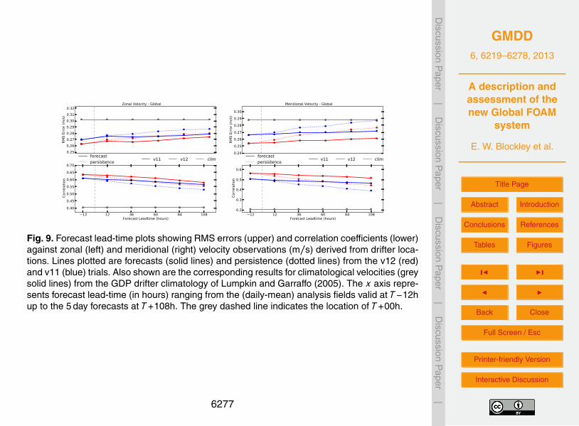
GMDD6, 6219–6278, 2013


system


Title Page



Tables Figures

J I

J I

Back Close

Full Screen / Esc



Discussion

Paper

|D

iscussionP

aper|

Discussion

Paper

|D

iscussionP

aper|


0.25

0.26

0.27

0.28

0.29

0.30

0.31

0.32

RM

S E

rror

(m/s

)

forecastpersistence

12 12 36 60 84 108Forecast Leadtime (hours)

0.40

0.45

0.50

0.55

0.60

0.65

0.70

Corr

ela

tion

v11 v12 clim

Zonal Velocity - Global

0.24

0.25

0.26

0.27

0.28

0.29

0.30

RM

S E

rror

(m/s

)

forecastpersistence

12 12 36 60 84 108Forecast Leadtime (hours)

0.2

0.3

0.4

0.5

0.6

Corr

ela

tion

v11 v12 clim

Meridional Velocity - Global

Fig. 9. Forecast lead-time plots showing RMS errors (upper) and correlation coefficients (lower) against zonal (left) and meridional (right)velocity observations (m/s) derived from drifter locations. Lines plotted are forecasts (solid lines) and persistence (dotted lines) from thev12 (red) and v11 (blue) trials. Also shown are the corresponding results for climatological velocities (grey solid lines) from the GDP drifterclimatology of Lumpkin and Garraffo (2005). The x-axis represents forecast lead-time (in hours) ranging from the (daily-mean) analysisfields valid at T-12h up to the 5-day forecasts at T+108h. The grey dashed line indicates the location of T+00h.

in keeping with the fact that, by design, OSTIA produces ananalysis that is smoother than the true surface temperature,particularly in areas of sharp fronts (Donlon et al., 2012). Thev12 SLA also compares well with the AVISO product butdoes not quite capture the high intensity of the anticyclonicfeatures at (22◦ E, 39.5◦ S) and (27.5◦ E, 36◦ S). Additionallythe cyclonic structure at (17◦ E, 36–38◦ S) is underestimatedin both the v12 and v11 systems as is the northwards projec-tion to the west of the retroflection at 15◦ E.

The free model does not do a bad job here and, to a cer-tain extent, does represent the large-scale flow quite well. Itdoes not manage to capture the finer scale features seen inthe observations and assimilative runs though which is notsurprising given that ORCA025 is only an eddy permitting,rather than a fully eddy resolving, model.

Although velocities are not assimilated in any of the sys-tems the near-surface velocity fields in the (v12/v11) assim-ilative runs are considerably closer to the OSCAR productthan are those of the free run. This will have been caused bythe SLA assimilation successfully constraining the circula-tion.

5 Summary and future plans

In this paper recent developments to the Met Office FOAMsystem have been introduced, the new FOAM v12 systemhas been described and changes relative to the previous v11FOAM system have been highlighted. Results have been pre-sented from three 2-year FOAM experiments and the perfor-mance of the new v12 system has been compared to the old

v11 system and a free-running, non-assimilative v12 systemto investigate the respective impacts of the v12 upgrade andthe data assimilation. Assessments have focused on the anal-ysis of FGAT innovations throughout the reanalysis periodas well as daily-mean model-observation match-ups derivedfrom a series of 5-day forecasts spun-off the assimilative tri-als for 8 months during the assessment period (Jan, Apr, Juland Oct each year). An additional qualitative assessment ofthe reanalysis surface fields has been performed by compar-ing 2D spatial maps of SSH, SST and surface currents fromall three FOAM trials against AVISO, OSTIA, and OSCARgridded observational products.

Results show that surface fields, and in particular surfacetemperature, are generally improved in the new v12 systemwith global SST and SSH RMS errors of 0.45 ◦C and 7.4 cmrespectively. Comparisons with gridded observational prod-ucts suggest that the v12 system provides a better representa-tion of mesoscale features in the extra-tropics — an improve-ment that will have been caused primarily by the shorterhorizontal correlation lengthscales used within NEMOVAR(Waters et al., 2013b). Data assimilation is shown to have apositive effect on the surface fields with a reduction in sur-face temperature biases and correction of a long-term driftin surface height. Comparisons with gridded data sets showa considerable improvement for the assimilative runs and anincreased spatial structure to the surface fields.

The quality of near-surface (< 80m) temperature andsalinity fields is also improved in the new v12 system. Theincreased accuracy of near-surface temperatures is caused bythe move to NEMOVAR and the associated improvements to

Fig. 9. Forecast lead-time plots showing RMS errors (upper) and correlation coefficients (lower)against zonal (left) and meridional (right) velocity observations (m/s) derived from drifter loca-tions. Lines plotted are forecasts (solid lines) and persistence (dotted lines) from the v12 (red)and v11 (blue) trials. Also shown are the corresponding results for climatological velocities (greysolid lines) from the GDP drifter climatology of Lumpkin and Garraffo (2005). The x axis repre-sents forecast lead-time (in hours) ranging from the (daily-mean) analysis fields valid at T−12hup to the 5 day forecasts at T+108h. The grey dashed line indicates the location of T+00h.

6277





GMDD6, 6219–6278, 2013


system


Title Page



Tables Figures

J I

J I

Back Close

Full Screen / Esc



Discussion

Paper

|D

iscussionP

aper|

Discussion

Paper

|D

iscussionP

aper|


0.044

0.0440.044

0.044 0.04

4

0.044

0.04

4

0.04

4

0.180

0.180

0.180

0.180

0.18

0

0.180

0.316

0.316

0.316

0.316

0.31

6

0.316

0.452

0.45

2

0.452

0.452

0.452

0.588

0.588

0.588

0.58

8

0.588

0.588

0.724

0.724

0.72

4

0.724

0.86

0

0.860

-0.466

-0.466

-0.330

-0.330

-0.3

30

-0.330

-0.194

-0.1

94

-0.194

-0.194

-0.194

-0.194

-0.058

-0.058

-0.058

-0.0

58

-0.058

-0.058

-0.058

-0.058

-0.058-0.058

16 20 24 28 32

16 20 24 28 32

-42

-40

-38

-36

-34

-32

-42-40

-38-36

-34-32v12

8.28

8.28

9.409.409.40

9.40

9.40

10.52

10.52

10.52

10.52

10.52

11.6411.64

11.6411.64

11.64

11.64

12.7612.7

6

12.76

12.76

12.76

12.76

13.8

813.88

13.88

13.88

13.88

15.00

15.00

15.00

15.00

15.00

16.12

16.12

16.12

16.1

2

16.1

2

16.12

16.12

16.12

17.24

17.2

4

17.24

17.24

17.2418.36

18.36

18.36

18.36

19.48

19.48

19.48

20.60

20.60

21.72

16 20 24 28 32

16 20 24 28 32

-42

-40

-38

-36

-34

-32

-42-40

-38-36

-34-32v12

16 20 24 28 32

16 20 24 28 32

-42

-40

-38

-36

-34

-32

-42-40

-38-36

-34-32v12

0.0440.044

0.044

0.044

0.044

0.044

0.0440.044

0.04

4

0.044

0.04

4

0.04

4

0.180

0.180

0.180

0.18

0

0.18

0

0.180

0.180

0.180

0.180

0.316

0.316

0.3160.316

0.316

0.31

6

0.316

0.31

6

0.452

0.452

0.45

20.452

0.452

0.452

0.45

2

0.452

0.45

2

0.58

8

0.588

0.588

0.58

80.588

0.588

0.588

0.58

8

0.58

8

0.72

4

0.724

0.724

0.724

0.72

4

0.724

0.724

0.72

4

0.86

0

0.860

0.860

0.860

0.860

0.996

0.99

6

-0.4

66

-0.466

-0.3

30

-0.3

30

-0.3

30

-0.330

-0.330

-0.194

-0.1

94

-0.1

94

-0.194

-0.194

-0.1

94

-0.1

94 -0.194

-0.1

94

-0.194

-0.194

-0.1

94

-0.1

94

-0.194

-0.058

-0.058

-0.058

-0.058

-0.058

-0.058

-0.0

58

-0.0

58

-0.0

58

-0.058

16 20 24 28 32

16 20 24 28 32

-42

-40

-38

-36

-34

-32

-42-40

-38-36

-34-32AVISO

8.28

8.28

8.28

8.28

9.40

9.40

9.40

9.40

9.40

10.52

10.5210.52

10.5

2

10.52

11.6411.64

11.64

11.6

4

11.6

4

11.64

12.7612.7612.76

12.7

6

12.76

13.88

13.8813.88

13.88

13.88

13.8

8

15.00

15.0015.00

15.00

15.0

0

16.12

16.12

16.12

16.12

16.12

16.1

2

16.12

17.24

17.24

17.24

17.24

17.2

4

18.36

18.36

18.36

18.36

19.48

19.48

19.48

20.60

20.60

16 20 24 28 32

16 20 24 28 32

-42

-40

-38

-36

-34

-32

-42-40

-38-36

-34-32OSTIA

16 20 24 28 32

16 20 24 28 32

-42

-40

-38

-36

-34

-32

-42-40

-38-36

-34-32OSCAR

0.0440.044

0.044

0.044

0.044

0.044

0.044

0.1800.180

0.18

0

0.180

0.180

0.18

0

0.3160.316

0.31

6

0.31

6

0.31

6

0.316 0.316

0.31

6

0.452

0.452

0.45

2

0.452

0.452

0.58

8 0.588

0.588

0.588

0.58

8

0.588

0.72

4

0.72

4

0.724

0.724

0.72

4

0.724

0.724

0.86

0

0.860

0.86

0

-0.466

-0.466

-0.330

-0.330

-0.330

-0.330

-0.194

-0.194

-0.194

-0.1

94

-0.194

-0.1

94

-0.194

-0.1

94

-0.194

-0.058

-0.058

-0.058

-0.0

58

-0.058

-0.058

-0.058

-0.058

-0.0

58

-0.0

58

-0.058

-0.058

-0.058

-0.0

58

16 20 24 28 32

16 20 24 28 32

-42

-40

-38

-36

-34

-32

-42-40

-38-36

-34-32v11

8.28

8.28

9.409.409.40

9.40

9.40

10.52

10.5210.5

2

10.52

10.52

11.64

11.6411.64

11.6

4

11.64

11.64

12.76

12.7612.76

12.76

12.76

12.76

13.88

13.88

13.88

13.88

13.88

13.88

15.00

15.00

15.00

15.00

15.00

15.00

16.1216.12

16.12

16.12

16.12

16.12

16.12

17.24

17.24

17.2

4

17.24

17.24

17.2418.36

18.36

18.36

18.36

18.36

19.48

19.48

19.4820.60

20.6

0

16 20 24 28 32

16 20 24 28 32

-42

-40

-38

-36

-34

-32

-42-40

-38-36

-34-32v11

16 20 24 28 32

16 20 24 28 32

-42

-40

-38

-36

-34

-32

-42-40

-38-36

-34-32v11

0.044

0.044

0.044

0.044

0.044

0.044

0.044

0.1800.180

0.18

0

0.180

0.1800.

180

0.316

0.316

0.316

0.316

0.316

0.452

0.452

0.45

2

0.452

0.452 0.588

0.588

0.588

0.588

0.724

-0.466

-0.466

-0.330

-0.330

-0.330

-0.330

-0.194

-0.1

94

-0.19

4

-0.194

-0.194

-0.194

-0.1

94

-0.058

-0.058

-0.058

-0.058

-0.058

-0.058-0.058

-0.058

16 20 24 28 32

16 20 24 28 32

-42

-40

-38

-36

-34

-32

-42-40

-38-36

-34-32

free

-0.5 -0.4 -0.3 -0.2 -0.1 0 0.1 0.2 0.3 0.4 0.5 0.6 0.7 0.8 0.9 1 1.1 1.2

8.28

8.28

8.28

9.409.40

9.40

9.40

10.52

10.5210.52

10.52

10.52

11.64

11.6

4

11.64

11.64

11.64

12.76

12.7

6

12.76

12.76

12.76

13.88

13.88

13.88

13.88

13.88

13.88

13.8

8

15.00

15.00

15.0

0

15.00

15.00

15.00

16.12

16.12

16.1

2

16.12

16.12

16.12

16.12

17.2

4

17.24

17.24

17.24

17.24

18.36

18.36

18.3

6

18.36

18.36

19.48

19.4819.48

20.60

20.6

0

21.72

16 20 24 28 32

16 20 24 28 32

-42

-40

-38

-36

-34

-32

-42-40

-38-36

-34-32

free

8 9 10 11 12 13 14 15 16 17 18 19 20 21 22

16 20 24 28 32

16 20 24 28 32

-42

-40

-38

-36

-34

-32

-42-40

-38-36

-34-32

free

0 0.08 0.16 0.24 0.32 0.40 0.48 0.56 0.64 0.72 0.80

SSH SST CRT

Fig. 10. An array of monthly-mean gridded contour plots over the Agulhas retroflection region (longitude: 12◦ E – 36◦ E; latitude: 31◦ S– 43◦ S) for September 2012. Sea surface height (left column : m) and temperature (centre column : ◦C) are plotted as coloured contoursand overlaid with black contour lines. For the SSH plots solid black lines denote positive contour values and broken white lines are usedfor negative values. Surface currents (right column : m/s) are displayed as coloured contours of current intensity (speed) with white arrowsoverlaid to show direction. Output from the v12, v11 and free trials are plotted in the 1st, 3rd and 4th rows respectively whilst the 2nd rowplots show the gridded observational products: AVISO SSH, OSTIA SST and OSCAR surface currents. Model currents shown (i.e. v12, v11and free) are total integrated velocity over the top 15m.

SST. However the salinity improvement is in contrast to theresults of Waters et al. (2013b) and is driven by the surfaceboundary condition upgrade to use CORE bulk formulae.

Temperature at 100 m is slightly degraded in the v12 sys-tem and this seems to be a result of the present version of theNEMOVAR assimilation scheme not being able to constraina persistent model bias quite as well as the old OCNASMscheme did. Although sub-surface salinity is better globallyand in the North Atlantic, there is a slight degradation in mostother regions. In particular, salinity is worse in the South-ern Ocean throughout most of the water column. Althoughthe shorter horizontal correlation lengthscales employed by

NEMOVAR allow for tighter matching of mesoscale fea-tures, they also make it harder for the assimilation to con-strain the tracer fields at depth owing to the sparsity of sub-surface observations (Waters et al., 2013b). This is thought tobe responsible for the degradation of temperature and salin-ity at depths below 80m. Further research is required herebut it is hoped that the extension of NEMOVAR to includemultiple horizontal lengthscales (as used in OCNASM) willbetter constrain the tracer fields at depth.

Assessment of the forecast fields shows that the v12 SSTfields remain better than the v11 system and considerablybetter than climatology throughout the 5-day forecasts. How-

Fig. 10. An array of monthly-mean gridded contour plots over the Agulhas retroflection region(longitude: 12◦ E–36◦ E; latitude: 31◦ S–43◦ S) for September 2012. Sea surface height (left col-umn: m) and temperature (centre column: ◦C) are plotted as coloured contours and overlaidwith black contour lines. For the SSH plots solid black lines denote positive contour valuesand broken white lines are used for negative values. Surface currents (right column: m s−1)are displayed as coloured contours of current intensity (speed) with white arrows overlaid toshow direction. Output from the v12, v11 and free trials are plotted in the 1st, 3rd and 4th rowsrespectively whilst the 2nd row plots show the gridded observational products: AVISO SSH,OSTIA SST and OSCAR surface currents. Model currents shown (i.e. v12, v11 and free) aretotal integrated velocity over the top 15 m.

6278





a description and assessment of the new global foam - gmdd

Documents