a differential forms approach to electromagnetics in anisotropic media
TRANSCRIPT
A DIFFERENTIAL FORMS APPROACH TOELECTROMAGNETICS IN ANISOTROPIC MEDIA
A Dissertation
Submitted to the
Department of Electrical and Computer Engineering
Brigham Young University
In Partial Fulfillment
of the Requirements for the Degree
Doctor of Philosophy
c© Karl F. Warnick 2003
by
Karl F. Warnick
February, 1997
A DIFFERENTIAL FORMS APPROACH TO ELECTROMAGNETICS INANISOTROPIC MEDIA
Karl F. Warnick
Department of Electrical and Computer Engineering
Ph.D. Degree, February, 1997
ABSTRACT
The behavior of electromagnetic fields in an inhomogeneous, anisotropic med-ium can be characterized by a tensor Green function for the electric field. In this disserta-tion, a new formalism for tensor Green functions using the calculus of differential forms isproposed. Using this formalism, the scalar Green function for isotropic media is general-ized to an anisotropic, inhomogeneous medium. An integral equation is obtained relatingthis simpler Green function to the desired Green function for the electric field, generalizingthe standard technique for construction of the Green function for the isotropic case from thescalar Green function. This treatment also leads to a new integral equation for the electricfield which is a direct generalization of a standard free space result. For the special caseof a biaxial medium, a paraxial approximation for the Green function is used to obtain theGaussian beam solutions. A straightforward analysis breaks down for beams propagatingalong two singular directions, or optical axes, so these directions are investigated specially.The associated phenomenon of internal conical refraction is known to yield a circular inten-sity pattern with a dark ring in its center; this analysis predicts the appearence of additionaldark rings in the pattern.
COMMITTEE APPROVAL:David V. Arnold, Committee Chairman
Richard H. Selfridge, Committee Member
David G. Long, Committee Member
Michael A. Jensen, Committee Member
B. Kent Harrison, Committee Member
Michael D. Rice, Graduate Coordinator
This dissertation by Karl F. Warnick is accepted in its present form by the Department
of Electrical and Computer Engineering of Brigham Young University as satisfying the
dissertation requirement for the degree of Doctor of Philosophy.
David V. Arnold, Committee Chairman
Richard H. Selfridge, Committee Member
David G. Long, Committee Member
Michael A. Jensen, Committee Member
B. Kent Harrison, Committee Member
Date Michael D. Rice, Graduate Coordinator
ii
DEDICATION
To my wife Shauna for her support and faith in me.
iii
ACKNOWLEDGMENTS
I would like to thank especially Dr. David V. Arnold, for his encouragement,support, and friendship. His insights provided the foundation for many of the results ofthis dissertation. Dr. Richard H. Selfridge was the first in the Department of Electrical andComputer Engineering to become interested in differential forms, and helped in obtainingresults and understanding on which this work is based. I thank him for many discussionsand insights and for his support of my efforts. I thank also Dr. David Long, Dr. GayleMiner, Dr. Kent Harrison, and Dr. Michael Jensen for assisting my work and taking time todiscuss issues and questions that came up in connection with this research. I am grateful toall of the department faculty and staff for providing a pleasant and supportive environmentduring my time at Brigham Young University. Finally, I acknowledge the National ScienceFoundation for funding this research through a Graduate Fellowship.
iv
Contents
Dedication iii
Acknowledgments iv
1 Introduction 1
2 Background 72.1 Green Function Methods for Complex Media . . . . . . . . . . . . . . . . 72.2 Present Approach . . . . . . . . . . . . . . . . . . . . . . . . . . . . . . . 82.3 Survey of the Calculus of Differential Forms . . . . . . . . . . . . . . . . . 92.4 Introduction to the Calculus of Differential Forms . . . . . . . . . . . . . . 11
2.4.1 Degree of a Differential Form; Exterior Product . . . . . . . . . . . 112.4.2 Maxwell’s Laws in Integral Form . . . . . . . . . . . . . . . . . . 132.4.3 The Hodge Star Operator and the Constitutive Relations . . . . . . 142.4.4 The Exterior Derivative and Maxwell’s Laws in Point Form . . . . 142.4.5 The Interior Product and Boundary Conditions . . . . . . . . . . . 162.4.6 Integration by Pullback . . . . . . . . . . . . . . . . . . . . . . . . 18
2.5 Summary . . . . . . . . . . . . . . . . . . . . . . . . . . . . . . . . . . . 19
3 Green Forms for Anisotropic, Inhomogeneous Media 203.1 The Hodge Star Operator for a Complex Medium . . . . . . . . . . . . . . 213.2 The Green Form for the Electric Field . . . . . . . . . . . . . . . . . . . . 27
3.2.1 Boundary Conditions . . . . . . . . . . . . . . . . . . . . . . . . . 303.2.2 Symmetry and Self-Adjointness Conditions . . . . . . . . . . . . . 32
3.3 Green Form for the Anisotropic Helmholtz Equation . . . . . . . . . . . . 353.3.1 Integral Relationship BetweenG andg . . . . . . . . . . . . . . . 363.3.2 Symmetric Permeability Tensor . . . . . . . . . . . . . . . . . . . 37
3.4 Electrically Inhomogeneous Media . . . . . . . . . . . . . . . . . . . . . . 383.5 Homogeneous Media . . . . . . . . . . . . . . . . . . . . . . . . . . . . . 38
3.5.1 Exact Solution for the Helmholtz Green Form . . . . . . . . . . . . 403.6 Summary . . . . . . . . . . . . . . . . . . . . . . . . . . . . . . . . . . . 43
4 Electric Field Integral Equation 454.1 Applications . . . . . . . . . . . . . . . . . . . . . . . . . . . . . . . . . . 45
4.1.1 Homogeneous Media . . . . . . . . . . . . . . . . . . . . . . . . . 464.1.2 Inhomogeneous Media . . . . . . . . . . . . . . . . . . . . . . . . 47
4.2 Correspondence with Free Space Results . . . . . . . . . . . . . . . . . . . 504.2.1 Plane Wave Solutions . . . . . . . . . . . . . . . . . . . . . . . . . 55
4.3 Singularity of the Helmholtz Green Form . . . . . . . . . . . . . . . . . . 554.4 Summary . . . . . . . . . . . . . . . . . . . . . . . . . . . . . . . . . . . 58
v

5 Gaussian Beams in Biaxial Media 605.1 Introduction . . . . . . . . . . . . . . . . . . . . . . . . . . . . . . . . . . 605.2 Spectral Decomposition of the Green Form . . . . . . . . . . . . . . . . . 615.3 Paraxial Approximation of the Green Form . . . . . . . . . . . . . . . . . 635.4 Gaussian Beams . . . . . . . . . . . . . . . . . . . . . . . . . . . . . . . . 66
6 Internal Conical Refraction 696.1 Introduction . . . . . . . . . . . . . . . . . . . . . . . . . . . . . . . . . . 696.2 Propagation Along an Optical Axis . . . . . . . . . . . . . . . . . . . . . . 716.3 Numerical Validation and Interpretation of Results . . . . . . . . . . . . . 786.4 Summary . . . . . . . . . . . . . . . . . . . . . . . . . . . . . . . . . . . 82
7 Conclusion 837.1 Further Research . . . . . . . . . . . . . . . . . . . . . . . . . . . . . . . 84
A Boundary Conditions Using Differential Forms 94A.1 Derivation . . . . . . . . . . . . . . . . . . . . . . . . . . . . . . . . . . . 94
A.1.1 Representing Surfaces With 1-forms . . . . . . . . . . . . . . . . . 94A.1.2 The Boundary Projection Operator . . . . . . . . . . . . . . . . . . 95A.1.3 Orientation of Sources . . . . . . . . . . . . . . . . . . . . . . . . 97
A.2 Boundary Decomposition of Forms . . . . . . . . . . . . . . . . . . . . . . 98
B Teaching Electromagnetic Field Theory Using Differential Forms 101B.1 Introduction . . . . . . . . . . . . . . . . . . . . . . . . . . . . . . . . . . 101
B.1.1 Development of Differential Forms . . . . . . . . . . . . . . . . . 102B.1.2 Differential Forms in EM Theory . . . . . . . . . . . . . . . . . . 102B.1.3 Pedagogical Advantages of Differential Forms . . . . . . . . . . . 104B.1.4 Outline . . . . . . . . . . . . . . . . . . . . . . . . . . . . . . . . 105
B.2 Differential Forms and the Electromagnetic Field . . . . . . . . . . . . . . 105B.2.1 Representing the Electromagnetic Field with Differential Forms . . 106B.2.2 1-Forms; Field Intensity . . . . . . . . . . . . . . . . . . . . . . . 106B.2.3 2-Forms; Flux Density and Current Density . . . . . . . . . . . . . 110B.2.4 3-Forms; Charge Density . . . . . . . . . . . . . . . . . . . . . . . 111B.2.5 0-forms; Scalar Potential . . . . . . . . . . . . . . . . . . . . . . . 112B.2.6 Summary . . . . . . . . . . . . . . . . . . . . . . . . . . . . . . . 112
B.3 Maxwell’s Laws in Integral Form . . . . . . . . . . . . . . . . . . . . . . . 113B.3.1 Ampere’s and Faraday’s Laws . . . . . . . . . . . . . . . . . . . . 113B.3.2 Gauss’s Laws . . . . . . . . . . . . . . . . . . . . . . . . . . . . . 114B.3.3 Constitutive Relations and the Star Operator . . . . . . . . . . . . . 115B.3.4 The Exterior Product and the Poynting 2-form . . . . . . . . . . . . 117B.3.5 Energy Density . . . . . . . . . . . . . . . . . . . . . . . . . . . . 120
B.4 Curvilinear Coordinate Systems . . . . . . . . . . . . . . . . . . . . . . . 121B.4.1 Cylindrical Coordinates . . . . . . . . . . . . . . . . . . . . . . . 121B.4.2 Spherical Coordinates . . . . . . . . . . . . . . . . . . . . . . . . 122B.4.3 Generalized Orthogonal Coordinates . . . . . . . . . . . . . . . . . 123
vi
B.5 Electrostatics and Magnetostatics . . . . . . . . . . . . . . . . . . . . . . . 124B.5.1 Point Charge . . . . . . . . . . . . . . . . . . . . . . . . . . . . . 124B.5.2 Line Charge . . . . . . . . . . . . . . . . . . . . . . . . . . . . . . 125B.5.3 Line Current . . . . . . . . . . . . . . . . . . . . . . . . . . . . . 126
B.6 The Exterior Derivative and Maxwell’s Laws in Point Form . . . . . . . . . 127B.6.1 Exterior Derivative of 0-forms . . . . . . . . . . . . . . . . . . . . 128B.6.2 Exterior Derivative of 1-forms . . . . . . . . . . . . . . . . . . . . 128B.6.3 Exterior Derivative of 2-forms . . . . . . . . . . . . . . . . . . . . 129B.6.4 Properties of the Exterior Derivative . . . . . . . . . . . . . . . . . 129B.6.5 The Generalized Stokes Theorem . . . . . . . . . . . . . . . . . . 130B.6.6 Faraday’s and Ampere’s Laws in Point Form . . . . . . . . . . . . 132B.6.7 Gauss’s Laws in Point Form . . . . . . . . . . . . . . . . . . . . . 133B.6.8 Poynting’s Theorem . . . . . . . . . . . . . . . . . . . . . . . . . 133B.6.9 Integrating Forms by Pullback . . . . . . . . . . . . . . . . . . . . 134B.6.10 Existence of Graphical Representations . . . . . . . . . . . . . . . 136B.6.11 Summary . . . . . . . . . . . . . . . . . . . . . . . . . . . . . . . 136
B.7 The Interior Product and Boundary Conditions . . . . . . . . . . . . . . . . 137B.7.1 The Interior Product . . . . . . . . . . . . . . . . . . . . . . . . . 137B.7.2 Boundary Conditions . . . . . . . . . . . . . . . . . . . . . . . . . 139B.7.3 Surface Current . . . . . . . . . . . . . . . . . . . . . . . . . . . . 139B.7.4 Surface Charge . . . . . . . . . . . . . . . . . . . . . . . . . . . . 141
B.8 Conclusion . . . . . . . . . . . . . . . . . . . . . . . . . . . . . . . . . . 143
vii
List of Tables
B.1 Differential forms of each degree. . . . . . . . . . . . . . . . . . . . . . . 106B.2 The differential forms that represent fields and sources. . . . . . . . . . . . 107
viii
List of Figures
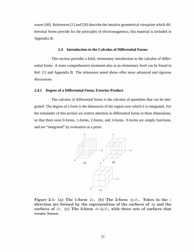
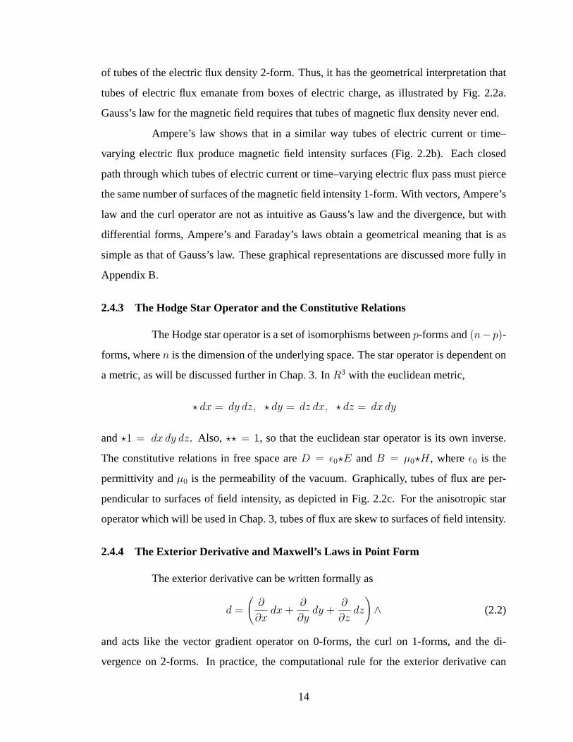
2.1 (a) The 1-formdx. (b) The 2-form dy dz. Tubes in thez direction areformed by the superposition of the surfaces ofdy and the surfaces ofdz.(c) The 3-formdx dy dz, with three sets of surfaces that create boxes. . . . 11
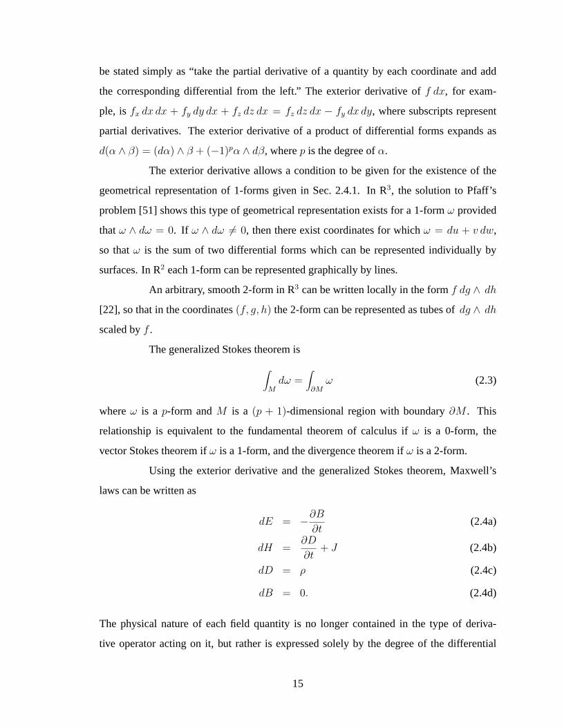
2.2 (a) Gauss’s law: boxes of electric charge produce tubes of electric flux. (b)Ampere’s law: tubes of current produce magnetic field surfaces. (c) Tubesof D are perpendicular to surfaces ofE, sinceD = ε0?E. . . . . . . . . . 13
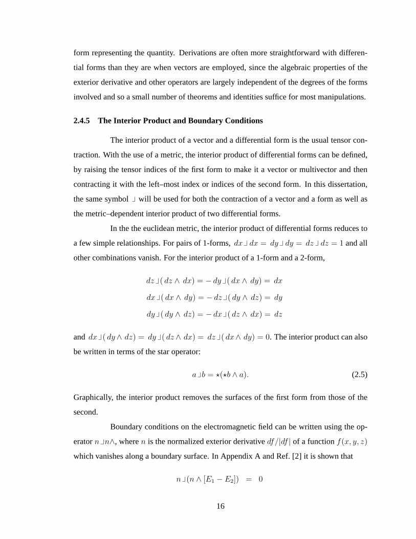
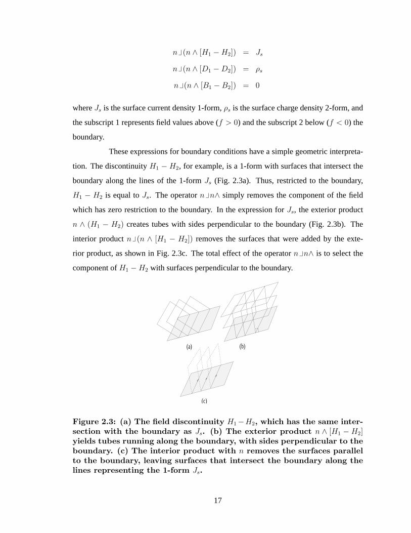
2.3 (a) The field discontinuityH1 −H2, which has the same intersection withthe boundary asJs. (b) The exterior productn ∧ [H1 − H2] yields tubesrunning along the boundary, with sides perpendicular to the boundary. (c)The interior product withn removes the surfaces parallel to the boundary,leaving surfaces that intersect the boundary along the lines representing the1-formJs. . . . . . . . . . . . . . . . . . . . . . . . . . . . . . . . . . . 17
6.1 Geometry of internal conical refraction. Thez direction is an optical axis.Normals to the wave surface at the singular point generate the cone of re-fraction. . . . . . . . . . . . . . . . . . . . . . . . . . . . . . . . . . . . . 72
6.2 A circular cross section of the cone of refraction.b1 is the distance from(x, y, z) to the cone in thex-y plane. . . . . . . . . . . . . . . . . . . . . . 77
6.3 Magnitude ofE/E0 for Aragonite,z = 10 cm, beam waist 34µm, andwavelength .6328µm. The solid line is computed by numerical integration.On the same scale the percentage error is shown as a dashed line. Incidentpolarization is in thex direction. The cone of refraction intersects the xaxis atx = −3.5 mm. . . . . . . . . . . . . . . . . . . . . . . . . . . . . . 78
6.4 Magnitude ofF (1 + iq, b). The local minimum along theb = 0 axis pro-duces the dark ring in the intensity pattern of conical refraction.b > 0corresponds to the interior of the cone andb < 0 to the exterior. . . . . . . . 79
6.5 Magnitude ofE/E0 for Aragonite,z = 1 cm, w0 = 18 µm, andλ =.6328 µm. The singularity of (6.27) at the center of the cone of refractionappears atx = −.175 mm. Incident polarization is in thex direction. . . . 79
6.6 Same as Fig. 6.3, except that dashed lines are magnitudes of the internal andexternal contributions taken separately and the solid line is total intensityas given by Eq. (6.27). . . . . . . . . . . . . . . . . . . . . . . . . . . . . 81
B.1 (a) The 1-formdx, with surfaces perpendicular to thex axis and infinite inthey andz directions. (b) The 1-form2 dz, with surfaces perpendicular tothez-axis and spaced two per unit distance in thez direction. (c) A moregeneral 1-form, with curved surfaces and surfaces that end or meet eachother. . . . . . . . . . . . . . . . . . . . . . . . . . . . . . . . . . . . . . 108
B.2 A path piercing four surfaces of a 1-form. The integral of the 1-form overthe path is four. . . . . . . . . . . . . . . . . . . . . . . . . . . . . . . . . 109
B.3 (a) The 2-formdx dy, with tubes in thez direction. (b) Four tubes of a2-form pass through a surface, so that the integral of the 2-form over thesurface is four. . . . . . . . . . . . . . . . . . . . . . . . . . . . . . . . . 111
ix

B.4 The 3-formdx dy dz, with cubes of side equal to one. The cubes fill allspace. . . . . . . . . . . . . . . . . . . . . . . . . . . . . . . . . . . . . . 112
B.5 (a) A graphical representation of Ampere’s law: tubes of current producesurfaces of magnetic field intensity. Any loop around the three tubes ofJmust pierce three surfaces ofH. (b) A cross section of the same magneticfield using vectors. The vector field appears to “curl” everywhere, eventhough the field has nonzero curl only at the location of the current. . . . . 114
B.6 A graphical representation of Gauss’s law for the electric flux density:boxes ofρ produce tubes ofD. . . . . . . . . . . . . . . . . . . . . . . . 115
B.7 The star operator relates 1-form surfaces to perpendicular 2-form tubes. . . 116B.8 The Poynting power flow 2-formS = E ∧ H. Surfaces of the 1-formsE
andH are the sides of the tubes ofS. . . . . . . . . . . . . . . . . . . . . 119B.9 The 3-form2w due to fields inside a parallel plate capacitor with oppositely
charged plates. The surfaces ofE are parallel to the top and bottom plates.The tubes ofD extend vertically from charges on one plate to oppositecharges on the other. The tubes and surfaces intersect to form cubes of2ω,one of which is outlined in the figure. . . . . . . . . . . . . . . . . . . . . 120
B.10 Surfaces of (a)dρ, (b) dφ scaled by3/π, and (c)dz. . . . . . . . . . . . . 122B.11 Surfaces of (a)dr, (b) dθ scaled by10/π, and (c)dφ scaled by3/π. . . . 123B.12 Electric flux density due to a point charge. Tubes ofD extend away from
the charge. . . . . . . . . . . . . . . . . . . . . . . . . . . . . . . . . . . 125B.13 Electric flux density due to a line charge. Tubes ofD extend radially away
from the vertical line of charge. . . . . . . . . . . . . . . . . . . . . . . . 126B.14 Magnetic field intensityH due to a line current. . . . . . . . . . . . . . . . 127B.15 The Stokes theorem forω a 1-form. (a) The loopbdM pierces three of the
surfaces ofω. (b) Three tubes ofdω pass through any surfaceM boundedby the loopbdM . . . . . . . . . . . . . . . . . . . . . . . . . . . . . . . 131
B.16 Stokes theorem forω a 2-form. (a) Four tubes of the 2-formω pass througha surface. (b) The same number of boxes of the 3-formdω lie inside thesurface. . . . . . . . . . . . . . . . . . . . . . . . . . . . . . . . . . . . . 132
B.17 (a) The 1-formH1 − H2. (b) The 2-formn ∧ (H1 − H2). (c) The 1-formJs, represented by lines on the boundary. Current flows along the lines. . . 140
B.18 (a) The 2-formD1 − D2. (b) The 3-formn ∧ (D1 − D2), with sides per-pendicular to the boundary. (c) The 2-formρs, represented by boxes on theboundary. . . . . . . . . . . . . . . . . . . . . . . . . . . . . . . . . . . . 142
x

Chapter 1
INTRODUCTION
Electromagnetic fields interact with the materials in which they exist. On the
atomic scale, the interactions between fields and particles can be extremely complex, but
on a macroscopic scale, the influence of a medium on fields can be modelled by modifying
the constitutive relations between the electric and magnetic field intensity and the associ-
ated flux densities. These constitutive relations, together with Maxwell’s laws, govern the
propagation of fields in materials. A medium for which the relationship between field and
flux density depends on the direction of field intensity is an anisotropic medium. If the con-
stitutive relations depend on position, then the medium is inhomogeneous. A bianisotropic
medium is one in which electric and magnetic fields are coupled by the constitutive rela-
tions. In this dissertation I consider the behavior of electromagnetic fields in an anisotropic,
inhomogeneous medium. Bianisotropic, nonlinear, and spatially dispersive media are not
considered. The term complex media is often used to denote the class of materials of
the most general type, but “complex media” or “general media” will be used here to de-
note the limited category under consideration. The most general constitutive relation to be
treated are possibly position dependent, linear relationships of the formDi = εij(r)Ej and
Bi = µij(r)Hj, whereεij is the permittivity tensor andµij is the permeability tensor. In
the general derivations of Chapters 3 and 4, the only restriction placed on the constitutive
tensors is that they must be non–singular. Special cases are treated thereafter. Chapters
5 and 6 deal with biaxial materials, which are homogeneous, magnetically isotropic, and
have a diagonalizable permittivity tensor with three unique eigenvalues. I consider only
time–harmonic (e−iωt) fields, so that effects due to temporal dispersion are neglected. Al-
though many of the general results given in this dissertation are coordinate–free, I employ
rectangular coordinates almost exclusively when dealing with expressions in component
form.
1

Numerous types of materials fall into the class treated in this dissertation. Aniso-
tropic media are employed in electromagnetic devices for modulation and control of sig-
nals, especially those materials for which the anisotropy can be influenced by application of
a static or slowly varying electric field and devices which employ polarization–dependent
effects to control microwave and optical signals. Anisotropic effects of the ionosphere
must be studied in order to understand the behavior of radio waves for which transmission
is affected by this region of the atmosphere. Problems involving inhomogeneous media are
ubiquitous, and range from investigations of interaction between a biological object and
a radiating antenna to statistical analysis of effects on signal propagation due to random
fluctuation of atmospheric properties. Inhomogeneous media arise in a variety of remote
sensing applications, and their effects must be quantified in order to effectively evaluate
and interpret data obtained by detection of signals radiated or scattered by natural or artifi-
cial materials. Inhomogeneous materials such as graded index fibers are often employed in
optical systems. Problems for which the medium could be considered both inhomogeneous
and anisotropic include the scattering problem for bounded anisotropic materials of various
shapes, layered anisotropic media, or anisotropic coatings.
Methods for analysis of fields in complex media are manifold. Possible ap-
proaches include computational algorithms for solving differential and integral equations
as well as analytical approaches specialized to particular problems. The particular method
to be extended and applied here is the theory of the tensor Green function for the electric
field. Maxwell’s laws can be solved for an arbitrary source configuration and a specified
boundary condition if an appropriate tensor Green function is available. The tensor Green
function essentially represents the electric field produced by an infinitesimal current source
of arbitrary orientation and location. If this Green function is known, then the fields due
to a given source can be obtained by direct integration, so that the Green function can
be thought of as completely characterizing the electromagnetic properties of a particular
medium.
For a general medium, a closed form representation of the Green function has
not been obtained. For an inhomogeneous medium, the problem of determining the Green
function is especially difficult, since information about the variation of the medium over
2
the entire region of interest must be incorporated into the Green function. Even for a biaxial
medium, the Green function can only be given in closed form asymptotically. The present
understanding of Green functions for complex media is far from complete, and the research
reported in this dissertation is intended to advance this area of electromagnetic field theory.
Chapter 2 is devoted to a study of previous work on Green functions for com-
plex media and an introduction to the primary tool used in this dissertation, the calculus
of differential forms. The power of differential forms as a tool for electromagnetics is the
foundation of the results of this dissertation. As outlined briefly in Chap. 2 and in detail in
Appendix B and Ref. [1], the calculus of differential forms offers both algebraic and geo-
metrical advantages over traditional vector analysis. With differential forms, many vector
identities and theorems are reduced to simple, algebraic properties. This makes differen-
tial forms ideal in searching for new theoretical approaches, since manipulations are often
more transparent and less tedious than they would be if the usual notation were employed.
Differential forms also allow field quantities and the laws they obey to be visualized in an
intuitive manner. This is valuable in research since problems can be understood and solved
first visually and then mathematically. The geometrical representation for electromagnetic
boundary conditions given in Chap. 2, for example, is naturally related to the mathematical
expression derived in Ref. [2] and Appendix A.
In order to employ the calculus of differential forms to treat the theory of elec-
tromagnetic Green functions, I represent the tensor Green function as a double differential
form, rather than as a dyadic. The utility of double forms for the case of free space has been
demonstrated in Ref. [3], where it is shown that differential forms make key expressions
more concise and easier to apply in some respects than their dyadic formulations. In order
to treat a general medium, I construct in Chap. 3 Hodge star operators from the permittivity
and permeability tensors. The new formalism arising from the use of these star operators
yields two benefits: first, the same few fundamental theorems and algebraic properties of
the calculus of differential forms which are used to treat electromagnetics in free space can
be employed for complex media with only minor modification. Second, expressions extend
3

in a more obvious way to the inhomogeneous, anisotropic case, facilitating the generaliza-
tion of free space results to complex media. Some results generalize to a complex medium
simply by reinterpreting the star operators which are already present in the expressions.
After using this formalism to define the Green form for the electric field, I re-
cover known results for the electric field in terms of the Green form, impressed sources,
and boundary values of the fields due to sources external to the region of interest. Unlike
previous treatments, this derivation follows the pattern of the standard, formal theory of
Green functions by obtaining key results from a generalization of Green’s theorem. With
the derivation cast into this form, the origins of symmetry and self–adjointness properties
of the Green form and the associated differential operator become clear. The treatment
also elucidates the role of boundary conditions in determining the properties of the Green
function and the associated differential operator.
For a homogeneous, isotropic medium, the tensor Green function can be con-
structed from a simpler Green function associated with the scalar Helmholtz equation.
Similar techniques have been sought for anisotropic media with limited success in cer-
tain special cases, as will be reviewed in Chap. 2. The primary intent of Chapter 3 is to
generalize this type of construction. While I do not obtain a closed form solution for the
Green function, the treatment does yield a result that is a rather direct generalization of the
free space method. Using the wave operator of the calculus of differential forms, I gen-
eralize to a complex medium the scalar Helmholtz equation and the associated free space
Green function. The associated Green function is a double form rather than a scalar quan-
tity, but is still simpler than the Green form for the electric field. This Helmholtz Green
form can be obtained analytically for an unbounded, homogeneous, anisotropic medium.
For an isotropic medium, it reduces to a double form with the usual scalar Green function
as the diagonal component. Following introduction of the Helmholtz Green form, the cen-
tral result of this work is derived: a relationship between the Helmholtz Green form and
the Green form for the electric field. In free space, the Green form for the electric field
can be expressed in terms of the scalar Green function and its derivatives. For a complex
medium, this relationship becomes an integral equation. Although the integral equation
4
does not reduce directly to the free space expression, the two constructions are very similar
in form. The work contained in Chap. 3 has been reported in Ref. [4].
Chapter 4 treats in more detail an integral equation for the electric field in terms
of the Helmholtz Green form of the previous chapter. The equivalence of this integral equa-
tion with a standard result for the electric field due to sources in an isotropic, homogeneous
medium is demonstrated. The isotropic expression is manipulated into a form that gener-
alizes directly to the case of a complex medium. I contrast this integral equation with the
usual integral equation method for complex media, and discuss cases where the present
approach may have advantage over the usual method. I also give a principal value interpre-
tation for integrals involving derivatives of the Helmholtz Green form, which is required in
order to implement the integral equation numerically.
Following these general considerations, I specialize to the case of a biaxial
medium. Chapter 5 treats the propagation of Gaussian beams in biaxial media. I give
the beam solutions and parameters in terms of the direction of propagation and the per-
mittivity of the medium. There are two singular directions, or optical axes, for which the
results of Chap. 5 break down. Narrow beams in these directions spread into a hollow cone.
This phenomenon is known as internal conical refraction. In Chap. 6, I give a special anal-
ysis of beams for these directions, obtaining an expression for field intensities that yields
new features of internal conical refraction not discerned by previous theories. The material
in this chapter is also reported in Ref. [5]. It has long been known that the characteristic,
annular intensity pattern produced by internal conical refraction of a narrow beam exhibits
in its center a fine, dark ring. This dark ring has been observed and explained theoretically.
The analysis presented here indicates the existence of secondary dark rings concentric to
the primary dark ring on the interior of the intensity pattern. For a biaxial medium, these
secondary fringes have apparently not been observed or predicted, although similar dark
rings have been reported for an optically active crystal [6]. I give quantitative results for
the field intensity at various parameter values and specify the parameter regime for which
this effect should appear.
In summary, the contributions of this dissertation to electromagnetic field theory
in general and the study of electromagnetic propagation in complex media are:
5
• A new formalism based on the Hodge star operator for electromagnetic Green func-
tions in complex media;
• A generalization of the Helmholtz equation to anisotropic, inhomogeneous media,
the definition of the associated Green form, and the solution for the Helmholtz Green
form for the case of a homogeneous, anisotropic medium;
• An integral equation relating the Green form for the electric field to the Helmholtz
Green form which generalizes the standard construction for the free space Green
function;
• A new electric field integral equation with kernel related to the Helmholtz Green
form which is a direct generalization of a standard free space result;
• A generalization of the free space Stratton–Chu formula to complex media;
• Explicit representation of Gaussian beam solutions for generic propagation directions
in a biaxial medium;
• A precise analysis of internal conical refraction of a Gaussian beam with wave direc-
tion along an optical axes of a biaxial medium, and the prediction of new structure in
the associated intensity pattern.
The results of this research include not only the solution of specific problems, but also a new
theoretical approach to the theory of anisotropic, inhomogeneous media, with the definition
of the Helmholtz Green form and integral equation relating the Green form for the electric
field to the Helmholtz Green form. There are many special cases for which approximate or
exact methods of solutions for this integral equation might be sought. Numerical methods
based on this equation might also be developed. In the conclusion to this dissertation,
several of the more obvious avenues for further work are noted.
6
Chapter 2
BACKGROUND
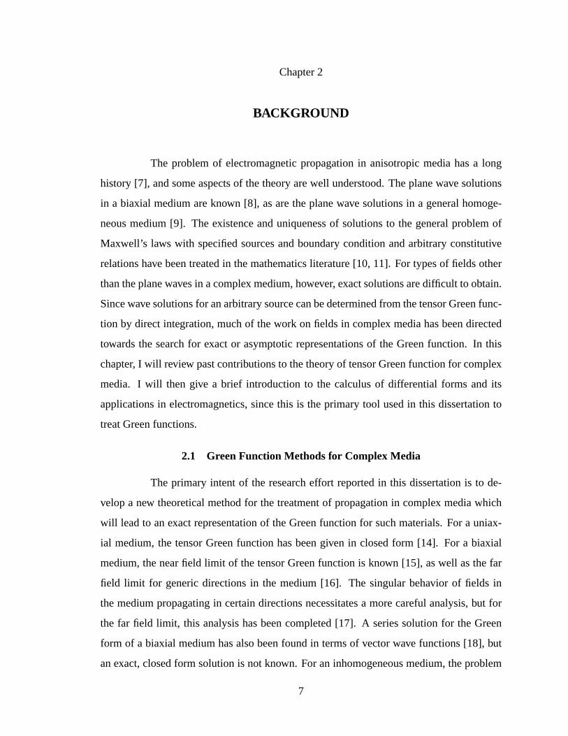
The problem of electromagnetic propagation in anisotropic media has a long
history [7], and some aspects of the theory are well understood. The plane wave solutions
in a biaxial medium are known [8], as are the plane wave solutions in a general homoge-
neous medium [9]. The existence and uniqueness of solutions to the general problem of
Maxwell’s laws with specified sources and boundary condition and arbitrary constitutive
relations have been treated in the mathematics literature [10, 11]. For types of fields other
than the plane waves in a complex medium, however, exact solutions are difficult to obtain.
Since wave solutions for an arbitrary source can be determined from the tensor Green func-
tion by direct integration, much of the work on fields in complex media has been directed
towards the search for exact or asymptotic representations of the Green function. In this
chapter, I will review past contributions to the theory of tensor Green function for complex
media. I will then give a brief introduction to the calculus of differential forms and its
applications in electromagnetics, since this is the primary tool used in this dissertation to
treat Green functions.
2.1 Green Function Methods for Complex Media
The primary intent of the research effort reported in this dissertation is to de-
velop a new theoretical method for the treatment of propagation in complex media which
will lead to an exact representation of the Green function for such materials. For a uniax-
ial medium, the tensor Green function has been given in closed form [14]. For a biaxial
medium, the near field limit of the tensor Green function is known [15], as well as the far
field limit for generic directions in the medium [16]. The singular behavior of fields in
the medium propagating in certain directions necessitates a more careful analysis, but for
the far field limit, this analysis has been completed [17]. A series solution for the Green
form of a biaxial medium has also been found in terms of vector wave functions [18], but
an exact, closed form solution is not known. For an inhomogeneous medium, the problem
7

of finding the Green function is even more difficult than for a homogeneous, anisotropic
medium. Closed form representations must be sought using methods specialized to partic-
ular types of inhomogeneity, although general numerical methods for determination of the
Green function for inhomogeneous media are available [19].
As noted in the introduction, the main result of this dissertation is a generaliza-
tion of the free space construction of the tensor Green function for the electric field in terms
of a simpler Green function which can be obtained exactly. This type of representation has
been sought by other researchers, with success for certain limits or types of materials. Wei-
glhofer gives the tensor Green function for a uniaxial medium in closed form in terms of
scalar Green functions [14]. The Green function for an isotropic, inhomogeneous medium
has also been represented in terms of two simpler quantities satisfying coupled partial dif-
ferential equations [20]. The coupled equations can be solved for media varying only in
one dimension and in the limit of a weakly inhomogeneous medium. The far field limit
of the Green function for a biaxial medium can be expressed in terms of scalar quantities
which have the same form as the free space scalar Green function [16]. For a general com-
plex medium, however, a representation of this type for the tensor Green function has not
been has not been obtained in the past.
2.2 Present Approach
The theory developed in the following chapters relies on a new notation for
electromagnetics in complex media based on the calculus of differential forms. The tensor
Green function is represented as a double differential form, or Green form, as done for free
space by Thirring [12] in the spacetime representation and Ref. [3] in the3 + 1 represen-
tation. This approach can be extended to the case of a complex medium by embedding the
permittivity and permeability tensors into the Hodge star operator, rather than employing
them directly as tensor quantities. The use of the Hodge star operator to characterize mate-
rial properties was suggested in passing by Bamberg and Sternberg [13]. This new notation
allows the the identities and theorems of the calculus of differential forms which are used
for electromagnetics in free space to be applied to the theory of complex media.
8
The calculus of differential forms is widely used in various fields of physics and
mathematics, and its advantages over traditional vector and tensor methods have been noted
by many authors. In Sec. 2.3, I give a brief outline of some areas in which differential forms
are used, and then survey in more detail applications within the field of electromagnetics. In
order to provide background for the following chapters, Sec. 2.4 gives a brief introduction
to the quantities, operators, and key theorems of the calculus of differential forms, including
the exterior product, exterior derivative, the generalized Stokes theorem, and the interior
product. Maxwell’s laws, the free space constitutive relations, and boundary conditions are
represented using differential forms. These and other topics are treated in greater detail in
the Appendices.
2.3 Survey of the Calculus of Differential Forms
A differential form is a quantity that can be integrated, including differentials.
More precisely, a differential form is a fully covariant, fully antisymmetric tensor [21, 22].
The calculus of differential forms was developed from the exterior algebra of Grassman by
Cartan, Poincare and others in the early 1900’s, and like vector analysis is a self–contained
subset of tensor analysis.
Differential forms are used regularly in fields of physics such as general relativ-
ity [23], quantum field theory [24], thermodynamics [13], and mechanics [25]. A section
on differential forms is commonplace in mathematical physics texts [26, 27]. Differen-
tial forms have been applied to control theory by Hermann [28] and others. Systems of
differential forms are currently a prominent method in nonlinear control theory, and differ-
ential forms methods are used to search for symmetries of nonlinear differential equations
[29]. In applied electromagnetics, however, vector analysis was already entrenched by the
time the calculus of differential forms became widely known. In spite of this, a number of
authors have employed differential forms to treat various aspects of EM theory.
Aside from early papers in which Maxwell’s laws were originally written using
differential forms, the general relativity text by Misner, Thorne and Wheeler [23] is one
of the first works to emphasize the use of differential forms in electromagnetics. Since
the focus of the work is gravitation, applications of EM theory are not treated. Burke [30]
9

treats a range of mathematical physics topics. The chapter on electromagnetics gives an
elegant formulation of electromagnetic boundary conditions. Bamberg and Sternberg [13]
also develop various topics of mathematical physics. Maxwell’s equations appear as the
continuous limit of the laws of circuit theory expressed using discrete differential forms.
Other works include that of Ingarden and Jamiołkowksi [31], an electrodynam-
ics text using a mix of vectors and differential forms, and the advanced electrodynamics text
by Parrott [32]. Thirring [12] is a classical field theory text which treats general relativity
in addition to electromagnetics, but certain applied topics such as waveguides are included.
Thirring represents an electromagnetic Green function as a double differential form, and
derives a result analogous to that of Sec. 3.2 for free space in the spacetime formulation.
Flanders [25] is a standard reference on the mathematical aspects and applications of dif-
ferential forms.
Deschamp was among the first to suggest the use of differential forms in engi-
neering. His article [33] considers briefly several applications, such as Huygen’s principle
and reciprocity. The papers [34], [35], [36], [37], [38], [39], [40] are essentially simi-
lar to previous treatments, with additional applications such asCerenkov radiation [36]
or the Hertz potentials [39]. Reference [41] advocates a variational technique derived us-
ing differential forms for numerical solution of electromagnetics problems, and Ref. [42]
suggests a numerical method for computation of fields in elastic, conducting media based
on a method for the discretization of electromagnetic field and source differential forms.
Sasaki and Kasai [43] review the algebraic topology of the differential forms representing
the electromagnetic field. Burke also gives an interesting discussion of electromagnetics
using twisted differential forms [44], so that parity invariance is explicit and a “right–hand
rule” is not required. The papers [45, 46] employ differential forms to treat the relativistic
rotation of a charged particle in an electromagnetic field.
More recent work includes that of Kotiuga, who uses differential forms to solve
the problem of making cuts for magnetic scalar potentials in multiply connected regions
[47] and to provide a metric–independent functional for the variational solution of elec-
tromagnetic inverse problems. Baldwin has investigated the use of Clebsch potentials to
represent field quantities [48] and classified the principle linearly polarized electromagnetic
10
waves [49]. References [1] and [50] describe the intuitive geometrical viewpoint which dif-
ferential forms provide for the principles of electromagnetics; this material is included in
Appendix B.
2.4 Introduction to the Calculus of Differential Forms
This section provides a brief, elementary introduction to the calculus of differ-
ential forms. A more comprehensive treatment also at an elementary level can be found in
Ref. [1] and Appendix B. The references noted above offer more advanced and rigorous
discussions.
2.4.1 Degree of a Differential Form; Exterior Product
The calculus of differential forms is the calculus of quantities that can be inte-
grated. The degree of a form is the dimension of the region over which it is integrated. For
the remainder of this section we restrict attention to differential forms in three dimensions,
so that there exist 0-forms, 1-forms, 2-forms, and 3-forms. 0-forms are simply functions,
and are “integrated” by evaluation at a point.
z
x
y
z
x
y
y
(b)(a)
(c)
z
x
Figure 2.1: (a) The 1-form dx. (b) The 2-form dy dz. Tubes in the zdirection are formed by the superposition of the surfaces of dy and thesurfaces of dz. (c) The 3-form dx dy dz, with three sets of surfaces thatcreate boxes.
11
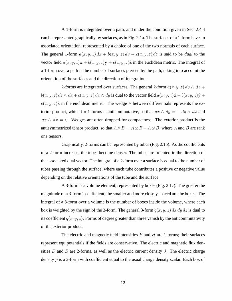
A 1-form is integrated over a path, and under the condition given in Sec. 2.4.4
can be represented graphically by surfaces, as in Fig. 2.1a. The surfaces of a 1-form have an
associated orientation, represented by a choice of one of the two normals of each surface.
The general 1-forma(x, y, z) dx + b(x, y, z) dy + c(x, y, z) dz is said to bedual to the
vector fielda(x, y, z)x + b(x, y, z)y + c(x, y, z)z in the euclidean metric. The integral of
a 1-form over a path is the number of surfaces pierced by the path, taking into account the
orientation of the surfaces and the direction of integration.
2-forms are integrated over surfaces. The general 2-forma(x, y, z) dy ∧ dz +
b(x, y, z) dz ∧ dx + c(x, y, z) dx∧ dy is dual to the vector fielda(x, y, z)x+ b(x, y, z)y +
c(x, y, z)z in the euclidean metric. The wedge∧ between differentials represents the ex-
terior product, which for 1-forms is anticommutative, so thatdx ∧ dy = − dy ∧ dx and
dx ∧ dx = 0. Wedges are often dropped for compactness. The exterior product is the
antisymmetrized tensor product, so thatA∧B = A⊗B−A⊗B, whereA andB are rank
one tensors.
Graphically, 2-forms can be represented by tubes (Fig. 2.1b). As the coefficients
of a 2-form increase, the tubes become denser. The tubes are oriented in the direction of
the associated dual vector. The integral of a 2-form over a surface is equal to the number of
tubes passing through the surface, where each tube contributes a positive or negative value
depending on the relative orientations of the tube and the surface.
A 3-form is a volume element, represented by boxes (Fig. 2.1c). The greater the
magnitude of a 3-form’s coefficient, the smaller and more closely spaced are the boxes. The
integral of a 3-form over a volume is the number of boxes inside the volume, where each
box is weighted by the sign of the 3-form. The general 3-formq(x, y, z) dx dy dz is dual to
its coefficientq(x, y, z). Forms of degree greater than three vanish by the anticommutativity
of the exterior product.
The electric and magnetic field intensitiesE andH are 1-forms; their surfaces
represent equipotentials if the fields are conservative. The electric and magnetic flux den-
sitiesD andB are 2-forms, as well as the electric current densityJ . The electric charge
densityρ is a 3-form with coefficient equal to the usual charge density scalar. Each box of
12

the 3-form represents a certain amount of charge. Each of these differential forms is dual
to the corresponding vector or scalar quantity.
2.4.2 Maxwell’s Laws in Integral Form
Using the differential forms for field and source quantities defined above, Maxwell’s
laws can be written as∮
PE = − d
dt
∫
AB
∮
PH =
d
dt
∫
AD +
∫
AJ
∮
SD =
∫
Vρ
∮
SB = 0 (2.1)
whereA is a surface bounded by a pathP andV is a volume bounded by a surfaceS. As
discussed in Appendix B, the units ofE andH areV andA, D andB have unitsC and
Wb, and the sourcesJ andρ have units ofA andC, since the differentials in these forms
are considered to have units of length.
(c)
(b)(a)
Figure 2.2: (a) Gauss’s law: boxes of electric charge produce tubes ofelectric flux. (b) Ampere’s law: tubes of current produce magnetic fieldsurfaces. (c) Tubes of D are perpendicular to surfaces of E, since D =ε0?E.
Gauss’s law for the electric field shows that a closed surface containing a certain
number of boxes of the electric charge density 3-form must be pierced by a like number
13
of tubes of the electric flux density 2-form. Thus, it has the geometrical interpretation that
tubes of electric flux emanate from boxes of electric charge, as illustrated by Fig. 2.2a.
Gauss’s law for the magnetic field requires that tubes of magnetic flux density never end.
Ampere’s law shows that in a similar way tubes of electric current or time–
varying electric flux produce magnetic field intensity surfaces (Fig. 2.2b). Each closed
path through which tubes of electric current or time–varying electric flux pass must pierce
the same number of surfaces of the magnetic field intensity 1-form. With vectors, Ampere’s
law and the curl operator are not as intuitive as Gauss’s law and the divergence, but with
differential forms, Ampere’s and Faraday’s laws obtain a geometrical meaning that is as
simple as that of Gauss’s law. These graphical representations are discussed more fully in
Appendix B.
2.4.3 The Hodge Star Operator and the Constitutive Relations
The Hodge star operator is a set of isomorphisms betweenp-forms and(n− p)-
forms, wheren is the dimension of the underlying space. The star operator is dependent on
a metric, as will be discussed further in Chap. 3. InR3 with the euclidean metric,
? dx = dy dz, ? dy = dz dx, ? dz = dx dy
and?1 = dx dy dz. Also, ?? = 1, so that the euclidean star operator is its own inverse.
The constitutive relations in free space areD = ε0?E andB = µ0?H, whereε0 is the
permittivity andµ0 is the permeability of the vacuum. Graphically, tubes of flux are per-
pendicular to surfaces of field intensity, as depicted in Fig. 2.2c. For the anisotropic star
operator which will be used in Chap. 3, tubes of flux are skew to surfaces of field intensity.
2.4.4 The Exterior Derivative and Maxwell’s Laws in Point Form
The exterior derivative can be written formally as
d =
(∂
∂xdx +
∂
∂ydy +
∂
∂zdz
)∧ (2.2)
and acts like the vector gradient operator on 0-forms, the curl on 1-forms, and the di-
vergence on 2-forms. In practice, the computational rule for the exterior derivative can
14
be stated simply as “take the partial derivative of a quantity by each coordinate and add
the corresponding differential from the left.” The exterior derivative off dx, for exam-
ple, isfx dx dx + fy dy dx + fz dz dx = fz dz dx − fy dx dy, where subscripts represent
partial derivatives. The exterior derivative of a product of differential forms expands as
d(α ∧ β) = (dα) ∧ β + (−1)pα ∧ dβ, wherep is the degree ofα.
The exterior derivative allows a condition to be given for the existence of the
geometrical representation of 1-forms given in Sec. 2.4.1. In R3, the solution to Pfaff’s
problem [51] shows this type of geometrical representation exists for a 1-formω provided
thatω ∧ dω = 0. If ω ∧ dω 6= 0, then there exist coordinates for whichω = du + v dw,
so thatω is the sum of two differential forms which can be represented individually by
surfaces. In R2 each 1-form can be represented graphically by lines.
An arbitrary, smooth 2-form in R3 can be written locally in the formf dg ∧ dh
[22], so that in the coordinates(f, g, h) the 2-form can be represented as tubes ofdg ∧ dh
scaled byf .
The generalized Stokes theorem is
∫
Mdω =
∫
∂Mω (2.3)
whereω is a p-form andM is a (p + 1)-dimensional region with boundary∂M . This
relationship is equivalent to the fundamental theorem of calculus ifω is a 0-form, the
vector Stokes theorem ifω is a 1-form, and the divergence theorem ifω is a 2-form.
Using the exterior derivative and the generalized Stokes theorem, Maxwell’s
laws can be written as
dE = −∂B
∂t(2.4a)
dH =∂D
∂t+ J (2.4b)
dD = ρ (2.4c)
dB = 0. (2.4d)
The physical nature of each field quantity is no longer contained in the type of deriva-
tive operator acting on it, but rather is expressed solely by the degree of the differential
15
form representing the quantity. Derivations are often more straightforward with differen-
tial forms than they are when vectors are employed, since the algebraic properties of the
exterior derivative and other operators are largely independent of the degrees of the forms
involved and so a small number of theorems and identities suffice for most manipulations.
2.4.5 The Interior Product and Boundary Conditions
The interior product of a vector and a differential form is the usual tensor con-
traction. With the use of a metric, the interior product of differential forms can be defined,
by raising the tensor indices of the first form to make it a vector or multivector and then
contracting it with the left–most index or indices of the second form. In this dissertation,
the same symbol will be used for both the contraction of a vector and a form as well as
the metric–dependent interior product of two differential forms.
In the the euclidean metric, the interior product of differential forms reduces to
a few simple relationships. For pairs of 1-forms,dx dx = dy dy = dz dz = 1 and all
other combinations vanish. For the interior product of a 1-form and a 2-form,
dz ( dz ∧ dx) = − dy ( dx ∧ dy) = dx
dx ( dx ∧ dy) = − dz ( dy ∧ dz) = dy
dy ( dy ∧ dz) = − dx ( dz ∧ dx) = dz
and dx ( dy∧ dz) = dy ( dz∧ dx) = dz ( dx∧ dy) = 0. The interior product can also
be written in terms of the star operator:
a b = ?(?b ∧ a). (2.5)
Graphically, the interior product removes the surfaces of the first form from those of the
second.
Boundary conditions on the electromagnetic field can be written using the op-
eratorn n∧, wheren is the normalized exterior derivativedf/|df | of a functionf(x, y, z)
which vanishes along a boundary surface. In Appendix A and Ref. [2] it is shown that
n (n ∧ [E1 − E2]) = 0
16
n (n ∧ [H1 −H2]) = Js
n (n ∧ [D1 −D2]) = ρs
n (n ∧ [B1 −B2]) = 0
whereJs is the surface current density 1-form,ρs is the surface charge density 2-form, and
the subscript 1 represents field values above (f > 0) and the subscript 2 below (f < 0) the
boundary.
These expressions for boundary conditions have a simple geometric interpreta-
tion. The discontinuityH1 − H2, for example, is a 1-form with surfaces that intersect the
boundary along the lines of the 1-formJs (Fig. 2.3a). Thus, restricted to the boundary,
H1 − H2 is equal toJs. The operatorn n∧ simply removes the component of the field
which has zero restriction to the boundary. In the expression forJs, the exterior product
n ∧ (H1 − H2) creates tubes with sides perpendicular to the boundary (Fig. 2.3b). The
interior productn (n ∧ [H1 − H2]) removes the surfaces that were added by the exte-
rior product, as shown in Fig. 2.3c. The total effect of the operatorn n∧ is to select the
component ofH1 −H2 with surfaces perpendicular to the boundary.
(a) (b)
(c)
Figure 2.3: (a) The field discontinuity H1−H2, which has the same inter-section with the boundary as Js. (b) The exterior product n ∧ [H1 −H2]yields tubes running along the boundary, with sides perpendicular to theboundary. (c) The interior product with n removes the surfaces parallelto the boundary, leaving surfaces that intersect the boundary along thelines representing the 1-form Js.
17
Unlike other differential forms of electromagnetics,Js is not dual to the usual
surface current density vectorJs. The expression for current through a pathP is
I =∫
PJs · (n× ds) (2.6)
wheren is a surface normal ands is tangent to the path. Using the 1-formJs, this simplifies
to
I =∫
PJs (2.7)
which is the obvious definition for a surface current quantity.
2.4.6 Integration by Pullback
Integrals of differential forms can be evaluated in a straightforward manner us-
ing the method of pullback. A vector field must be converted to a differential form before it
can be integrated. This accounts for the presence of an inner product in the path or surface
integral of vector field. The method of pullback is more natural, since neither a metric nor a
differential vector is required to evaluate an integral of a form. To integrate a 1-formω over
a pathP parameterized as(u(s), v(s), w(s)) in an arbitrary coordinate system(u, v, w), the
coordinatesu, v andw in the arguments of the coefficients as well as the differentials ofω
are replaced withu(s), v(s) andw(s). Jacobian factors enter automatically when the exte-
rior derivativesdu(s), dv(s), anddw(s) are computed. The result of the pullback operation
is a new 1-form which can be written asg(s) ds. This 1-form is the pullback ofω to the
pathP , and is integrated over the limits of the parameters of the path. Ifω is the 1-form
f(x, y, z) dx, for example, then the integral ofω over the pathP is
∫
Pω =
∫
Pf(x, y, z) dx
=∫ a
bf(u(s), v(s), w(s)) du(s)
=∫ a
bf(u(s), v(s), w(s))
∂u
∂sds.
Integration of a 2-form over a surface proceeds similarly, except that two parameterss and
t are necessary and the final integrand is a 2-form inds ∧ dt.
18

2.5 Summary
In this chapter, I have given a survey of various results contained in the literature
on the theory of electromagnetic Green functions which relate to the work reported in
this dissertation. I have also outlined the calculus of differential forms, since this will be
the primary tool to be employed in the following chapters. Chapter 3, which constitutes
the core of this dissertation, begins by generalizing the euclidean star operator of Sec.
2.4.3 to an asymmetric, complex metric, so that the star operator can be used to express
the constitutive relations for materials with arbitrary permeability and permittivity tensors.
This formalism enables other operators and theorems of the calculus of differential forms
to be used in obtaining the key result of this research: a new representation for the Green
function for the electric field for anisotropic, inhomogeneous media.
19

Chapter 3
GREEN FORMS FOR ANISOTROPIC, INHOMOGENEOUS
MEDIA
The goal of this chapter is to represent the tensor Green function for a complex
medium in terms of a simpler Green function which can be obtained exactly, generalizing
the standard construction method for the tensor Green function in free space. The material
given here is also contained in Ref. [4].
In order to derive this result, the tensor Green function is represented as a double
differential form. This method is employed to treat the special case of free space in Ref.
[3]. For the general case, in Sec. 3.1 material properties as characterized by the permittivity
and permeability tensors are embedded into the Hodge star operator. The usual definition
of the Hodge star operator must be modified for material tensors with negative or complex
determinants. In addition, the metric tensor from which the Hodge star operator is defined
is by definition symmetric. In order to employ the star operator to characterize media with
nonsymmetric material tensorsεij andµij, the definition of the Hodge star operator must
be extended in a formal manner. Fortunately, this new operator retains many of the same
properties as the usual, symmetric Hodge star operator, as demonstrated in Sec. 3.1. As
far as the derivations of this chapter are concerned, the primary difference between the
symmetric and nonsymmetric star operators is that the nonsymmetric star operator is not
proportional to its own inverse.
Following these preparatory derivations, in Sec. 3.2 I define the Green form
for the electric field and recover known results [52] for the electric field in terms of the
Green form and current sources. The derivation presented in this chapter is analogous to
the standard treatment of the general theory of Green functions [27]. As a result, the origins
of conventions used in the definition of the Green form and symmetry and self–adjointness
properties of the Green form and the associated partial differential operator become clear.
20
The reformulation of the tensor Green function as a double differential form
and the use of the Hodge star operator to express constitutive relations lead to a natural
generalization of the Helmholtz equation to anisotropic media. Unlike the Green form for
the electric field, the Green form for this generalized Helmholtz equation can be found
exactly for an important class of media, those which are homogeneous and anisotropic.
This class is quite general, since it includes biaxial media, lossy media, and nonreciprocal
media such as gyrotropic plasma. For an isotropic medium, the Helmholtz Green form
essentially reduces to the usual scalar Green function.
In Sec. 3.3 the main result of this chapter is given: an integral equation relating
the Green form for the electric field to the Helmholtz Green form. The kernel of this
integral equation consists of second order partial derivatives of the Helmholtz Green form.
The expression obtained in this chapter does not reduce directly to the usual result for
free space, since the usual result gives the electric field directly from the sources, while
the expression given here remains an integral equation even for free space. The integral
equation and the free space relationship, however, are very similar in form and have a clear
connection. The correspondence between the treatment of this chapter and standard free
space results is treated in Chap. 4.
By specializing to a homogeneous medium, this integral equation can be trans-
formed into the wavevector representation, leading to known expressions for the Fresnel
equation and the Fourier transform of the Green form for the electric field. The Neumann
series solution for the integral equation in the wavevector representation can be resummed,
yielding another type of representation for the Green form.
3.1 The Hodge Star Operator for a Complex Medium
In Sec. 2.4.3, the Hodge star operator was used to express the free space con-
stitutive relations. It was noted there that the Hodge star operator depends on a metric.
If this metric is related in the proper way to the permittivity and permeability tensors, the
free space constitutive relations of Sec. 2.4.3 can be generalized to the case of a complex
medium. In order to treat media which have nonsymmetric permittivity or permeability
tensors, however, the standard definition of the Hodge star operator must be extended in a
21
formal manner. The standard definition must also be modified if the determinants of the
material tensors are not real and positive, as can occur if a medium is lossy. After making
the necessary generalizations, I determine the inverse of the star operator, prove the theo-
rem ν ∧ ?λ = ?−1ν ∧ λ for p-forms ν andλ, and define the Laplace–de Rham or wave
operator.
The most commonly used definition for the Hodge star operator is that given by
Flanders [25] and Bamberg and Sternberg [13],
λ ∧ ν = (?λ, ν)σ (3.1)
whereν is ap-form,λ is an(n−p)-form,σ is the volume element?1 ≡√|g| dx1∧· · ·∧ dxn
and( , ) denotes the inner product ofp-forms induced by the metric tensorgij. Thirring
[12] gives an alternate definition,
?λ = λ σ (3.2)
where denotes the interior product on differential forms induced by the metricgij. These
two definitions can be shown to be equivalent using the relationshipλ ∧ ?ω = (λ ω)σ
whereλ andω arep-forms. Letν = ?ω. Then by making use of??ω = (−1)p(n−p)+sω,
Eq. (3.1) becomes
λ ∧ ν = (−1)p(n−p)+s(λ ?ν)σ. (3.3)
Thirring shows that(−1)p(n−p)+s(λ ?ν) is equal to the inner product of thep-forms ?λ
andν, so that this expression reduces to the definition (3.1). The text [23] on p. 97 also
defines a duality betweenp-forms and(n − p)-vectors. If the metric is used to lower the
indices of the(n − p)-vector, the resulting(n − p)-form is equivalent to that obtained by
applying the star operator to the originalp-form (note that the tensorε used in Ref. [23]
contains a factor of√|g|).
For the purposes of this chapter, an explicit definition of the star operator in
terms of a metric is most useful. For a simplep-form,
? dxi1 ∧ . . . ∧ dxip = gi1j1 . . . gipjpεj1...jn
√|g|
(n− p)!dxjp+1 ∧ · · · ∧ dxjn (3.4)
whereε is the Levi-Civita tensor,g is the determinant of the metric tensor,n is the dimen-
sion of space, andgij is the inverse metric. The derivation of this expression from (3.2) is
22
given as an exercise in Ref. [12]. For the euclidean metricδij, we recover the result given
in Sec. 2.4.3, that? dx = dy dz, ? dy = dz dx, ?dz = dx dy, and?1 = dx dy dz.
For symmetric, positive definite permittivity and permeability tensors, I define
?e using (3.4) with the inverse metricgij = εji/(detεij) and?h with gij = µji/(detµij).
The constitutive relations can then be written as
D = ?eE (3.5a)
B = ?hH. (3.5b)
Since a metric tensor is by definition symmetric, the definition (3.4) produces a true Hodge
star operator only ifgij = gji. By employing the expression formally with a nonsymmetric
gij, however, an operator is obtained which retains many of the useful properties of the
Hodge star operator. This allows the treatment given in this chapter to apply to nonrecipro-
cal media, for which the material tensors are nonsymmetric.
Due to the presence of the absolute value in the factor√|g| of Eq. (3.4), the
definition of the star operator must also be modified if the determinants of the material
tensors are not positive and real. I therefore define the star operator employed in this
chapter according to
? dxi1 ∧ . . . ∧ dxip = gi1j1 . . . gipjpεj1...jn
√g
(n− p)!dxjp+1 ∧ · · · ∧ dxjn . (3.6)
Using this definition, the constitutive relations (3.5) are valid for an anisotropic, inhomo-
geneous, nonbianisotropic, and linear medium. The operator obtained using the modified
definition, as well as its formal extension to a nonsymmetric tensorgij, is still referred to
as a star operator and given the same symbol? throughout this dissertation.
In rectangular coordinates, from Eq. (3.6) the star operator?e acts on an arbi-
trary 1-form in the obvious way, so that
?e(E1 dx + E2 dy + E3 dz) = (ε11E1 + ε12E2 + ε13E3) dy dz+
(ε21E1 + ε22E2 + ε23E3) dz dx+
(ε31E1 + ε32E2 + ε33E3) dx dy
(3.7)
23
where wedges between differentials are omitted. If the star operator?e is applied to a
2-form,
?e(D1 dy dz + D2 dz dx + D3 dx dy) = (ε11D1 + ε21D2 + ε31D3) dx+
(ε12D1 + ε22D2 + ε32D3) dy+
(ε13D1 + ε23D2 + ε33D3) dz
(3.8)
where theεij are components ofε−1. On 1-forms and 3-forms,
?e1 = (detεij) dx dy dz. (3.9)
The magnetic star operator?h behaves similarly.
For media with symmetric permeability and permittivity tensors,?e = ?e−1 and
?h = ?h−1. As can be seen by inspection of Eq. (3.8), in the nonsymmetric case the star
operator is no longer equal to its own inverse. As will be shown below, the inverse of the
star operator must in general be defined using (3.6) withgij replaced by its transposegji. I
give this transposed star operator the symbol?. The inverse star operator?e−1 = ?e is thus
obtained from (3.6) withgij = εij/(detεij) and?h−1 = ?h with gij = µij/(detµij).
I now prove that? is proportional to?−1 for a nonsymmetricgij by demonstrat-
ing the result for a simplep-form. The general case follows by linearity of the star operator.
Applying the definition (3.6) and using the shorthand notationdxi1 ∧· · ·∧ dxip = dxi1...ip,
?? dxi1...ip =g
p!(n− p)!gkp+1jp+1 · · · gknjngi1j1 · · · gipjpεkp+1...knk1...kpεj1...jn dxk1...kp .
Raising the indices ofεj1...jn and using the expression(1/g)δi1...inj1...jn
= εj1...jnεi1...in for the
permutation tensorδ in terms of the Levi–Civita tensor gives
?? dxi1...ip =1
p!(n− p)!gkp+1jp+1 · · · gknjngjp+1lp+1 · · · gjnlnδ
i1...iplp+1...lnkp+1...knk1...kp
dxk1...kp .
Using the definitiongijgjk = δk
i of the inverse metricgjk and permuting the indices
k1 . . . kn, this becomes
?? dxi1...ip =1
p!(n− p)!δ
kp+1
lp+1· · · δkn
ln(−1)p(n−p)δ
i1...iplp+1...lnk1...kn
dxk1...kp .
Summing the indiceslp+1 . . . ln gives
?? dxi1...ip =1
p!(n− p)!(−1)p(n−p)δ
i1...ipkp+1...kn
k1...kndxk1...kp .
24
Due to the antisymmetry of the permutation tensor, the quantityδi1...ipkp+1...kn
k1...knvanishes if
kn is equal to any ofi1, . . . , ip. Thus, there aren−p possible values forkn which contribute
to the summation overkn, so that the summation introduces a factor of(n − p). If kn−1 is
equal tokn or any ofi1, . . . , ip, the quantity also vanishes, sokn−1 hasn − p− 1 possible
values and thekn−1 summation yields a factor of(n − p − 1). By similar reasoning, after
summing overkp+1 throughkn−2, we have
?? dxi1...ip =1
p!(n− p)!(−1)p(n−p)(n− p)!δ
11...ipk1...kp
dxk1...kp .
Since both the permutation tensor anddxk1...kp are antisymmetric in the indicesk1 . . . kp,
the right–hand side consists ofp! copies of(1/p!)(−1)p(n−p) dxk1...kp , so that we have fi-
nally
?? dxi1...ip = (−1)p(n−p) dxi1...ip .
This proves the relationship
?−1 = (−1)p(n−p)? (3.10)
so that in R3, ?−1 = ?.
The identityν∧?λ = ?−1ν∧λ for p-formsν andλ is required for the derivations
in Sections 3.2 and 3.3. Thirring [12] proves the result for a symmetric star operator; I
generalize to the nonsymmetric case. The proof is given for simple forms and extends to
the general case by linearity. By the definition (3.6) of the star operator,
dxi1...ip ∧ ? dxj1...jp =
√g
(n− p)!gj1k1 · · · gjpkpεk1...kn dxi1...ipkp+1...kn . (3.11)
By rearranging the differentials using the antisymmetry of the exterior product of 1-forms,
dxi1...ip ∧ ? dxj1...jp =
√g
(n− p)!gj1k1 · · · gjpkpεk1...knεi1...ipkp+1...kn dx1...n.
This can be rewritten using the permutation tensorδ,
dxi1...ip ∧ ? dxj1...jp =
√g
(n− p)!gj1k1 · · · gjpkp
(n− p)!
gδ
i1...ipk1...kp
dx1...n.
Using an explicit representation [27] forδ, Eq. (3.11) becomes
dxi1...ip ∧ ? dxj1...jp =1√g
∑π
gj1iπ(1) · · · gjpiπ(p)sgn(π) dx1...n (3.12)
25
whereπ represents a permutation ofp objects. By rearranging the order of thegjkiπ(k), this
can be transformed into
dxi1...ip ∧ ? dxj1...jp =1√g
∑π
gjπ(1)i1 · · · gjπ(p)ipsgn(π) dx1...n
since for each permutationπ, the inverse permutation is also included in the summation.
Reversing the steps leading to Eq. (3.12), we find that
dxi1...ip ∧ ? dxj1...jp =
√g
(n− p)!gk1i1...kpipεk1...kn dxj1...jpkp+1...kn
=
√g
(n− p)!gk1i1...kpipεk1...kn(−1)p(n−p) dxkp+1...knj1...jp .
Using Eq. (3.10) together with the definition of? shows that
dxi1...ip ∧ ? dxj1...jp = ?−1dxi1...ip ∧ dxj1...jp . (3.13)
In R3 the inverse star operator in this expression can be replaced with?.
Finally, I extend the definition of the Laplace–de Rham or wave operator∆
to allow use of the nonsymmetric star operator.∆ is a generalization of the Laplacian.
Variation in sign conventions for∆ exists in the literature; the two alternatives are found
in Bamberg and Sternberg [13] and Thirring [12]. I choose Thirring’s definition, since it
agrees with the sign of the usual vector Laplacian. Accordingly, I define
∆α = (−1)n(p+1) [(−1)n?d?d + d?d?] α (3.14)
whereα is ap-form. This is equivalent to Thirring’s definition for a positive definite metric,
and for a constant metric with real eigenvalues it differs by the sign|g|/g = (−1)s, where
s is the signature ofgij. For a constant but otherwise arbitrary tensorgij, in a particular
coordinate system (3.14) reduces to
∆(ω dxi1...ip) = gij ∂2ω∂xi∂xj
dxi1...ip (3.15)
which becomes the usual expression for the Laplacian in the euclidean metricgij = gij =
δij.
26
3.2 The Green Form for the Electric Field
In this section, I define the Green form for the electric field, and derive an
expression for the observed electric field due to sources and external fields in terms of
the operator transpose of the Green form. I consider a linear, nonbianisotropic medium
with macroscopic electromagnetic properties characterized by invertible permittivity and
permeability tensorsεij(r) andµij(r). Maxwell’s laws are
dE = iωB (3.16a)
dH = −iωD + J (3.16b)
dD = ρ (3.16c)
dB = 0 (3.16d)
whereE andH are the electric and magnetic field intensity 1–forms,D andB are the
electric and magnetic flux density 2–forms,J is the electric current density 2–form, andρ
is the electric charge density 3–form. The constitutive relations areD = ?eE andB = ?hH
where the star operators?e and?h are defined in the previous section.
By applying the operator?hd?h to Faraday’s law and making use of the consti-
tutive relations and Ampere’s law, it can be shown that the electric fieldE satisfies
(−?hd?hd + ω2?h?e)E = −iω?hJ (3.17)
where the field quantities and the star operators are evaluated at the same point. The natural
Green double1⊗ 1 form G for this system of partial differential equations obeys the same
equation, but withiωJ replaced by an elementary or delta function source:
(−?hd?hd + ω2?h?e)G(r1, r2) = −?hδ(r1 − r2)I (3.18)
whereI is the unit2 ⊗ 1 form dy1 dz1 ⊗ dx2 + dz1 dx1 ⊗ dy2 + dx1 dy1 ⊗ dz2 and⊗denotes the tensor product. In rectangular coordinates, the Green form G has components
G(r1, r2) = G11 dx1 ⊗ dx2 + G12 dx1 ⊗ dy2 + G13 dx1 ⊗ dz2 +
G21 dy1 ⊗ dx2 + G22 dy1 ⊗ dy2 + G23 dy1 ⊗ dz2 + (3.19)
G31 dz1 ⊗ dx2 + G32 dz1 ⊗ dy2 + G33 dz1 ⊗ dz2.
27

where the coefficientsGij are functions ofr1 andr2. The tensor product⊗ is explicitly
included in these expressions to show that there is no exterior product between the differ-
entials of ther1 andr2 coordinate systems.
For an isotropic medium, the definition ofG becomes(− 1
µ?d
1
µ?d +
ω2ε
µ
)G(r1, r2) = − 1
µδ(r1 − r2)I (3.20)
whereε(r) andµ(r) are the scalar permittivity and permeability,? is the euclidean star
operator, andI is the unit1⊗1 form dx1⊗ dx2 + dy1⊗ dy2 + dz1⊗ dz2. The?h operator
acting from the left on both sides of (3.18) does not affect the definition ofG but is retained
since−?hd?hd is part of the Laplace-de Rham operator to be employed in Sec. 3.3.
In Eq. (3.18) and other expressions throughout this chapter, operators act on
the r1 coordinates unless otherwise noted. The star operator is in general a function of
position, and is evaluated at the position vector of the coordinate system corresponding
to the differentials on which it operates. Althoughr1 in the definition (3.18) represents
observation coordinates andr2 represents source coordinates, the standard approach to
Green function theory employed in this chapter naturally leads to a reversal of the roles of
the two coordinates. For reciprocal or lossless media, the symmetry relations for the Green
form obtained in Sec. 3.2.2 allow the coordinates to be interchanged.
I note here an important difference between this notation for double differen-
tial forms and the usual dyadic formulation. With double forms, the coordinate system to
which each differential belongs is explicitly specified. With dyadics, the unit vectors of
each component are not associated with a particular coordinate system. The information
contained in the coordinate dependence of the differentials is for dyadics contained in the
ordering of dot products with other quantities. With double forms, the ordering of factors is
not important as far as the coordinate dependence is concerned. Thus, with double differ-
ential forms the order of exterior products can be interchanged with a possible sign change
depending on the degrees of the forms. The operation corresponding to the transpose of a
dyadic becomes interchange of the coordinate dependence of the coefficients of a double
form, since the differentials are explicitly associated with the coordinate systems of the
arguments of the double form.
28
I define the formal transpose ofG to be the1⊗ 1 double formG satisfying
(−?hd?hd + ω2?h?e)G(r1, r2) = −?hδ(r1 − r2)I. (3.21)
This definition forG differs from Chew’s [52] definition for the dyadic Green function for
an anisotropic, inhomogeneous medium due to the presence of the operator?h on the left–
hand side of (3.21). In general,G is not the coordinate transpose of the double formG,
although in Sec. 3.2.1 it is shown thatG(r1, r2) = G(r2, r1) for certain types of boundary
conditions.
Let L andL represent the operators on the left hand sides of Eqs. (3.18) and
(3.21) respectively. In order to obtain the electric field in terms ofG, L andL must be such
that a relationship of the form
E1 ∧ (?hLE2)− E2 ∧ (?hLE1) = dP (3.22)
holds for arbitraryE1 andE2. This equation will lead to a generalized Green theorem, from
which symmetry and self–adjointness properties ofG for reciprocal and lossless media as
well as the solution for the electric field in terms of sources can be conveniently obtained.
The product rule for the exterior derivative [25],d(α∧β) = (dα)∧β+(−1)pα∧dβ, whereα is ap-form, and the relationshipν ∧?λ = ?ν ∧λ for p-formsν andλ obtained
in the previous section can be used to show that
d(E1 ∧ ?hdE2 + ?hdE1 ∧ E2) = d?hdE1 ∧ E2 − E1 ∧ d?hdE2. (3.23)
Applying this identity to (3.22) and using the definitions of L andL yields
P = E1 ∧ ?hdE2 + ?hdE1 ∧ E2 (3.24)
for the conjunct ofE1 andE2. Note that star operators cannot be moved across the exterior
products in this expression sinceE1 andE2 do not have the same degree asdE2 anddE1.
Integrating Eq. (3.22) over a volumeV1 and applying the generalized Stokes theorem∫
∂Vω =
∫
Vdω (3.25)
yields a generalization of Green’s theorem for the operators L andL,∫
V1
E1 ∧ (?hLE2)−∫
V1
E2 ∧ (?hLE1) =∫
∂V1
P (3.26)
29
where∂V1 denotes the boundary ofV1. This relationship shows thatL is the formal trans-
pose of L with respect to the inner product
< E1, E2 >=∫
VE1 ∧ ?hE2. (3.27)
If the surface term vanishes, then Eq. (3.26) becomes for L andL the definition of operator
transpose with respect to the inner product (3.27). The term formal refers to the possibility
that L andL may have different domains; the spaces of functions on which they act may,
for example, satisfy different boundary conditions.
I now wish to replaceE1(r1) with G(r1, r2) in (3.26). Yaghjian [53] shows that
for the case of an isotropic, homogeneous medium, the identity (3.26) with this substitution
is not valid if r1 = r2, sinceG(r1, r2) does not have continuous and unique second deriva-
tives atr1 = r2. This is due to ambiguity in the interpretation of the elementary sourceδI.
The resulting inconsistency can be resolved by employing an appropriate principal value
interpretation for volume integrals involvingG.
Proceeding with the substitution and applying the definition (3.21) produces the
generalized Huygens principle for anisotropic, inhomogeneous media,
E(r2) = iω∫
V1
G(r1, r2) ∧ J(r1) +∫
∂V1
[G(r1, r2) ∧ ?hdE(r1) + ?hdG(r1, r2) ∧ E(r1)
].
(3.28)
This is equivalent to the dyadic result given in [52]. Note the absence of surface normal
vectors in this expression. Normal components of the fields naturally do not contribute to
the surface integral term of (3.28).
3.2.1 Boundary Conditions
In this section, I seek to determine boundary conditions onE1 andE2 and the
Green forms such that the surface terms on the right–hand sides of (3.26) and (3.28) vanish.
I assume here thatG(r1, r2) as a function ofr1 satisfies the same boundary condition asE1
andG(r1, r2) as a function ofr1 satisfies the same boundary condition asE2. If the surface
contribution is zero, then replacingE1(r1) with G(r1, r2) and E2(r1) with G(r1, r3) in
(3.26) shows that
G(r3, r2) = G(r2, r3). (3.29)
30
Thus, for properly chosen boundary conditions,G is the coordinate transpose ofG. In
addition, the electric field as given by (3.28) will satisfy the same boundary condition as
G(r1, r2) as a function ofr2. By Eq. (3.29), the electric field will then satisfy the same
boundary condition asG(r1, r2) as a function ofr1. Boundary conditions for which the
surface contribution vanishes include radiation, Neumann (magnetically conducting), and
Dirichlet (electrically conducting). There are other boundary conditions for which the sur-
face term of (3.28) vanishes; this section treats only the simplest types.
Suppose thatE2 has the asymptotic behavior
limr→∞ r [dE2 − ik2 dr ∧ E2] = 0 (3.30a)
limr→∞ r(?h dr) ∧ E2 = 0 (3.30b)
limr→∞ r|E2| ≤ C (3.30c)
wherek2 is a bounded function ofr andC is a constant. LetE1 have the same behavior but
with k2 replaced withk1 in (3.30a) and?h replaced with?h in (3.30b). If∂V is a sphere
with radiusr, then
limr→∞
∣∣∣∣∫
∂VE1 ∧ ?h [dE2 − ik2 dr ∧ E2]
∣∣∣∣ ≤ limr→∞ 4πr2sup∂V |E1| sup∂V |dE2 − ik2 dr ∧ E2|
which vanishes by conditions (3.30a) and (3.30c). Using this result, we have that
limr→∞
∫
∂VP = lim
r→∞
∫
∂V[E1 ∧ ik2?h( dr ∧ E2) + ik1?h( dr ∧ E1) ∧ E2] . (3.31)
Using (2.5), the integrand can be rewritten using the interior product as
−ik2?h[E1˜( dr ∧ E2)] + ik1?h[E2 ( dr ∧ E1)]
where is the interior product induced by the metric of?h and ˜ is induced by?h. The
interior products expand by (A.7) to become
−ik2(E1˜ dr)?hE2 + ik1(E2 dr)?hE1 + ik2(E1˜E2)?h dr − ik1(E2 E1)?h dr.
By making use again of (2.5), this becomes
−ik2[?h(?h dr ∧ E1)]?hE2 + ik1[?h(?h dr ∧ E2)]?hE1
+ik2[?h(?hE2 ∧ E1)]?h dr − ik1[?h(?hE1 ∧ E2)]?h dr.
31

The first two terms of this expression vanish in the limit when integrated over∂V due to
the conditions (3.30b) and (3.30c), by an argument similar to that used in arriving at (3.31).
The second pair of terms can be written using (3.13) and (2.5) as
i(E2 E1)(k2?h − k1?h) dr.
In order for this to vanish, we must have that the permeability tensor is symmetric. We must
also have that the asymptotic forms ofE1 andE2 as expressed by (3.30a) be identical. A
sufficient condition for this is that the permittivity tensor be symmetric. Thus, for a medium
with symmetric permeability and permittivity tensors and outgoing fields satisfying the
conditions (3.30), the surface contribution to (3.26) vanishes. It remains to show for specific
types of media that the fields behave according to (3.30).
For electrically conducting boundary conditions, the 1-formsE1 and E2 are
oriented perpendicular to the boundary, so that ifn is a coordinate normal to the boundary,
thenE1 andE2 are proportional todn. The 2-formsE1 ∧ ?hdE2 and?hdE1 ∧E2 therefore
must each contain a factor ofdn. Since the surface integration is over all coordinates except
n, the boundary term of Eq. (3.26) vanishes.
For magnetically conducting boundary conditions, the 1-formH2 is oriented
perpendicular to the boundary, so thatH2 must be proportional todn. We have from
Faraday’s law and the constitutive relation forB that ?hdE2 = iωH2, so that?hdE2 is
also proportional todn. In general,E1 need not satisfy the same boundary condition as
E2 (physically,E2 satisfies Maxwell’s laws with constitutive relations as given by (3.5),
whereasE1 satisfies Maxwell’s laws with the magnetic constitutive relationB = ?hH). If
we require that?hdE1 be oriented perpendicular to the boundary, then this 1-form contains
a factor ofdn as well. For these conditions onE1 andE2, the boundary term of Eq. (3.26)
vanishes.
3.2.2 Symmetry and Self-Adjointness Conditions
The reaction of a fieldE and sourceJ is
< E, J >R=∫
VE ∧ J (3.32)
32
whereE is a 1-form andJ is a 2-form. The derivation of Eq. (3.26) together with the
relationship (3.17) show that if?h = ?h and?e = ?e, then
< E2, J1 >R − < E1, J2 >R=∫
∂V(E1 ∧H2 + H1 ∧ E2) (3.33)
whereE1 andE2 here are solutions of (3.17) with sourcesJ1 andJ2 respectively. This
is the Lorentz reciprocity theorem. For boundary conditions such that the right–hand side
vanishes, Eq. (3.33) reduces to the definition of reciprocity,< E2, J1 >R=< E1, J2 >R.
Thus, we recover the result that a medium is reciprocal if?h and?e are symmetric and the
fields satisfy boundary conditions such that the surface contribution of Eq. (3.33) vanishes.
Making use again of (3.17), we find from the definition of reciprocity that
∫
V1
E1 ∧ (?hLE2) =∫
V1
E2 ∧ (?hLE1) (3.34)
which shows that L is symmetric with respect to the inner product (3.27). ReplacingE1
with G(r1, r2) andE2 with G(r1, r3) in Eq. (3.34) gives the reciprocity relation [52]
G(r3, r2) = G(r2, r3) (3.35)
for a medium with symmetric permittivity and permeability tensors and fields satisfying
boundary conditions such that the surface contribution of Eq. (3.33) vanishes.
The energy imparted to the fieldE by the sourceJ is
< E, J >E=∫
VE∗ ∧ J. (3.36)
By slightly modifying the derivation of (3.26), one can show that if?e = ?e∗ and?h = ?h
∗,
then
< E1, J2 >E + < E2, J1 >∗E=
∫
∂V(H∗
1 ∧ E2 − E∗1 ∧H2) . (3.37)
The superscript∗ on ?e∗ and ?h
∗ denotes complex conjugation of the coefficients of the
permittivity and permeability tensors employed in the definitions of the star operators. For
a given sourceJ and associated fieldE, settingJ1 = J2 = J andE1 = E2 = E in (3.37)
yields
Re< E, J >E= −Re∫
∂VE ∧H∗. (3.38)
33
This equation represents a balance between energy imparted to the field by the sourceJ
and the power flow through the boundary ofV , so that the material in the regionV must
be lossless (note that this expression is the real part of Poynting’s theorem for a lossless
medium).
If in addition the boundary conditions are assumed to be such that the right–
hand side of (3.37) vanishes (so that no real power flows through the boundary ofV ), then
we have that
< E1, J2 >E= − < E2, J1 >∗E . (3.39)
For boundary conditions of this type, (3.39) can be taken as the definition of losslessness,
in the same way that< E2, J1 >R=< E1, J2 >R is the definition of reciprocity.
For a resonant frequency of a bounded region, (3.39) leads to an apparent con-
tradiction. At a resonance, the electric fieldE associated with a sourceJ is not uniquely
defined by Eq. (3.17). ForJ1 = J2 = J , E1 = E, andE2 = E+E0, whereE0 is a homoge-
neous solution to (3.17), Eq. (3.39) leads to the result that2Re< E, J >= − < E0, J >∗.
But (3.39) withE1 = E2 = E also requires that Re< E, J >= 0, so that< E0, J >
must vanish. The quantity< E0, J >, however, is in general not zero, since the current
J is arbitrary. The resolution of the contradiction lies in the observation that ifJ is not
orthogonal to all resonant modes ofV , power will continually be supplied to the field and
the assumption of steady state fields upon which the results of this section depend becomes
invalid.
Using the definition of L, Eq. (3.39) leads to∫
VE∗
1 ∧ (?hLE2) =[∫
VE∗
2 ∧ (?hLE1)]∗
. (3.40)
Thus, L is self–adjoint with respect to the inner product
< E1, E2 >=∫
VE∗
1 ∧ ?hE2 (3.41)
as has been shown by Chew [52]. ReplacingE1 with G(r1, r2) andE2 with G(r1, r3) in
(3.40) then yields
G∗(r3, r2) = G(r2, r3) (3.42)
so that the Green form for a lossless medium is hermitian if it satisfies boundary conditions
such that the surface contribution of Eq. (3.37) vanishes.
34

3.3 Green Form for the Anisotropic Helmholtz Equation
The derivative operator of Eq. (3.17) is not diagonal, making the solution for
the Green formG difficult to obtain. Addingd?hd?hE to both sides of Eq. (3.17) yields
(∆h + ω2?h?e)E = −iω?hJ + d?hd?hE (3.43)
where∆h is the wave operator in the metric due to the permeability of the medium and is
defined using Eq. (3.14) to be−?hd?d + d?hd?h. For a constant permeability tensor, the
operator∆h is diagonal and therefore simpler than the derivative operator of Eq. (3.17).
Since the operator on the left–hand side reduces in free space essentially to the Helmholtz
operator, I refer to (3.43) as the anisotropic Helmholtz equation. The corresponding Green
1⊗ 1 form g satisfies
(∆h + ω2?h?e)g(r1, r2) = −δ(r1 − r2)I (3.44)
where operators act on ther1 coordinate andI is the unit1 ⊗ 1 form. The Green form
g can be found in closed form for certain types of media for which no exact solution for
G is known. In free space,g = µ20g0I, whereg0 = eik0r/(4πr) is the usual scalar Green
function.
In Eq. (3.44) I have not included the?h operator on the right–hand side as was
done in Eq. (3.18). Since∆h is symmetric for constant?h, the additional?h operator does
not simplify the derivations of this section as it did in Sec. 3.2. The formal transpose ofg
is defined to be the2⊗ 1 Green formg which satisfies
(∆h + ω2?e?h)g(r1, r2) = −δ(r1 − r2)I (3.45)
whereI is the unit2 ⊗ 1 form. Note that the same derivative operator is employed in the
definitions ofg andg.
With the operators M= (∆h + ω2?h?e) andM = (∆h + ω2?e?h) appearing in
the definitions ofg andg, I seek to obtain a relationship of the form
C1 ∧ME2 − E2 ∧ MC1 = dQ (3.46)
whereE2 is an arbitrary 1-form andC1 is an arbitrary 2-form. The conjunctQ of E2 and
C1 defined by (3.46) can be shown to be
Q = ?hC1 ∧ ?hdE2 + ?hd?hC1 ∧ E2 + C1 ∧ ?hd?hE2 − ?hdC1 ∧ ?hE2. (3.47)
35
Integrating (3.46) over a volumeV and applying the generalized Stokes theorem yields
∫
VC1 ∧ME2 −
∫
VE2 ∧ MC1 =
∫
∂VQ. (3.48)
Substitutingg(r1, r2) for C1(r) and using Eqs. (3.43) and (3.45), we have
E(r2) = iω∫
V1
g(r1, r2) ∧ ?hJ(r1)−∫
V1
g(r1, r2) ∧ d?hd?hE(r1) +∫
∂V1
R (3.49)
whereR is
R = ?hg(r1, r2) ∧ ?hdE(r1) + ?hd?hg(r1, r2) ∧ E(r1)
+g(r1, r2) ∧ ?hd?hE(r1)− ?hdg(r1, r2) ∧ ?hE(r1).(3.50)
Integrating the second term on the right–hand side of (3.49) twice by parts cancels two of
the terms ofR, leaving
E(r2) = iω∫
V1
g(r1, r2) ∧ ?hJ(r1)−∫
V1
?hd?hdg(r1, r2) ∧ E(r1) +∫
∂V1
R1 (3.51)
where the operator?hd?hd acts on ther1 part of g and
R1 = ?hg(r1, r2) ∧ ?hdE(r1) + ?hd?hg(r1, r2) ∧ E(r1) (3.52)
is the integrand of the surface contribution.
If ?hg andE satisfy boundary conditions such as those described in Sec. 3.2.1,
so that the surface integral term of (3.51) vanishes, then we obtain the relationship
E(r2) = iω∫
V1
g(r1, r2) ∧ ?hJ(r1)−∫
V1
?hd?hdg(r1, r2) ∧ E(r1). (3.53)
This is a Fredholm integral equation of the second kind for the electric field in terms of the
sourceJ . As will be discussed in the following chapter, it may be possible to employ this
equation as a basis for numerical techniques for treating scattering problems in complex
media.
3.3.1 Integral Relationship BetweenG and g
Substitutingg(r1, r2) for C1 andG(r1, r3) for E2 in Eq. (3.48) and following a
procedure similar to the derivation of (3.51), I obtain the integral equation
G(r1, r2) = ?hg(r2, r1)−∫
V3
?hd?hdg(r3, r1) ∧G(r3, r2) (3.54)
36
where the derivatives act on ther3 coordinates ofg and surface terms have been neglected.
This expression generalizes to complex media the usual relationship between the scalar
Green function and the Green form for isotropic, homogeneous media [3].
By repeated substitution on (3.54) I obtain a formal series solution forG,
G = ?hg −∫
?hd?hdg ∧ ?hg +∫ ∫
?hd?hdg ∧ ?hd?hdg ∧ ?hg − · · · (3.55)
where coordinate dependence is suppressed. For free space, up to factors ofµ0 the second
term has components equal to the second partial derivatives ofeikr/(8πik). Beyond the
second term, increasingly high powers ofr appear, so that for larger the series diverges.
For a homogeneous medium, however, the wavevector representation of this series can be
resummed, as will be shown in Sec. 3.5.
3.3.2 Symmetric Permeability Tensor
For a symmetric permeability tensor, one can simplify expressions (3.51) and
(3.54) by absorbing a star operator?h into the definition ofg. I therefore employ the
modified definitions
(∆h + ω2?h?e)g = −?hδI (3.56a)
(∆h + ω2?h?e)g = −?hδI (3.56b)
whereg andg are1⊗ 1 forms andI is the unit2⊗ 1 form. One can now obtain an identity
of the form
E1 ∧ ?hM′E2 − E2 ∧ ?hM′E1 = dQ′ (3.57)
which replaces Eq. (3.46). By altering slightly the derivation given in the previous section,
one can show that Eq. (3.51) simplifies to
E(r2) = iω∫
V1
g(r1, r2) ∧ J(r1)−∫
V1
?hd?hd?hg(r1, r2) ∧ E(r1). (3.58)
The integral equation (3.54) becomes
G(r1, r2) = g(r1, r2)−∫
V3
?hd?hd?hg(r3, r2) ∧ G(r1, r3) (3.59)
for a symmetric?h operator and the modified definitions (3.56).
37
3.4 Electrically Inhomogeneous Media
The representation for the Green form (3.54), as well as the electric field integral
equation (3.53), connect scalar scattering by an isotropic, magnetically homogeneous, elec-
trically inhomogeneous medium with the electromagnetic scattering problem for the same
medium. Solution of Eq. (3.44) for the Helmholtz Green form reduces to the determination
of the usual scalar Green functiongs for the Helmholtz equation,
[∆ + k2(r1)]gs(r1, r2) = −δ(r1 − r2) (3.60)
wherek2(r) = ω2µ0ε(r). If the left–hand side of the definition (3.44) is multiplied byµ20,
the Helmholtz Green formg is then equal togsI. The scalar Green function can be found
analytically for certain types of inhomogeneous profiles, including the one–dimensional
variationk2(r) = k20(1 + az) [54] and the spherical profilek2(r) = k2
0(1 + ar2) [55],
leading to exact, closed form solutions for the Helmholtz Green form. If the Helmholtz
Green form is available in closed form, then the kernel of the integral equation (3.54) is
known and the integral equation becomes an exact representation of the Green form for
the electric field. The electric field integral equation (3.51) for electrically inhomogeneous
media will be discussed further in the following chapter.
3.5 Homogeneous Media
For a homogeneous medium, by spatial symmetry the components ofg are
shift–invariant functionsgij(r1 − r2). The integral in (3.54) becomes a convolution, so
that the Fourier transform of the integral is the product of the transforms of?hd?hdg and
G. The following transform relations can be used to obtain the wavevector representation
of ?hd?hdg. If a(r1, r2) is a2⊗ 1 form, b(r1, r2) is a1⊗ 1 form, andc(r1, r2) is a0-form
in ther1 coordinates, then
da(r1, r2) ←→ ikT a(k)
?hb(r1, r2) ←→ µT b(k)
dc(r1, r2) ←→ ikc(k)
wherek is the wavevector and derivatives act on ther1 coordinates. The coefficients of
the forms are functions ofr1 − r2, and the spatial Fourier transform is taken with respect
38

to this quantity. Throughout this section, the Fourier transforms of double forms will be
represented for convenience as matrices, and the same symbol used for both the physical
space representation of a double form and the matrix of the transforms of its components.
Matrix components are ordered according to Eq. (3.19).
The Fourier transform of?hd?hdg becomes−(1/detµ)µTkkT g. Since the ex-
terior product of this term withG acts on the first argument part rather than the second,
the matrix must be transposed in order to obtain the transform of the product. The spatial
Fourier transform of Eq. (3.54) is therefore
G = gT µ−1 +1
detµgTkkT µG. (3.61)
Solving forG, we obtain
G =
[µgT−1 − 1
detµµkkT µ
]−1
. (3.62)
Similarly, the Fourier transform of Eq. (3.45) shows that
g =
[1
detµ(kT µk)I − ω2εT µT−1
]−1
(3.63)
where I is the identity matrix. Eq. (3.18) leads to an alternate expression forG,
G =[−ΓµT−1Γ− ω2ε
]−1(3.64)
where
Γ =
0 −kz ky
kz 0 −kx
−ky kx 0
. (3.65)
Substituting (3.63) into (3.62) gives
G =
[− 1
detµµkkT µ +
1
detµ(kT µk)µ− ω2ε
]−1
(3.66)
which is equivalent to the result obtained in Ref. [9]. The poles ofG in the wavevector
representation represent plane wave solutions to (3.17), so that
det
[− 1
detµkkT µ +
1
detµ(kT µk)I − ω2µ−1ε
]= 0 (3.67)
is the Fresnel equation [9, 56] for an arbitrary homogeneous medium.
39
Finally, if the wave operator∆h is applied to a 1-form, the Fourier transform of
the definition (3.14) becomes
− 1
detµ(kT µk)I = µ−1ΓµT−1Γ− 1
detµkkT µ. (3.68)
This expression shows explicitly that the operator∆h is diagonal for an arbitrary (constant)
permeability tensor.
The wavevector representation of the series solution (3.55) forG can be re-
summed, leading to another representation for the Green form for the electric field. By
resubstitution, Eq. (3.61) can be transformed into
G = gT µ−1 +1
detµgTkkT µgT µ−1 +
1
detµgTkkT µ
1
detµgTkkT µgT µ−1 + · · · (3.69)
This can be rewritten as
G = gT µ−1 +1
detµgTk
1 +
1
detµkT µgTk +
(1
detµkT µgTk
)2
+ · · · kT µgT µ−1
(3.70)
where the series is now scalar and geometric. Summing the series yields
G = gT µ−1 +1
detµ
gT
1− 1detµkT µgTk
kkT µgT µ−1. (3.71)
For free space, the quantity inside square brackets is equal toµ20I/k
20, so that this expression
in physical space reduces up to factors ofµ0 to the usual expression for the Green form for
the electric field. The series in Eq. (3.70) is singular for values ofk that represent allowed
plane waves, so that1
detµkT µgTk = 1 (3.72)
is equivalent to the Fresnel equation (3.67).
3.5.1 Exact Solution for the Helmholtz Green Form
If µij is diagonalizable by a rotation, then the inverse transform ofg(k) can be
obtained in closed form. In this case, the kernel of the electric field integral equation (3.53)
and the Green form integral relationship (3.54) is known exactly. From Eq. (3.63),
g(r1, r2) =1
(2π)3
∫dkeik·r
[1
detµ(kT µk)I − ω2εT µT−1
]−1
(3.73)
40
wherer = r1−r2. By rotating the coordinate system so thatµij is diagonal and performing
a further change of variables such thatk′2 = kT µk/(detµ), this simplifies to
g(r1, r2) =detµ(2π)3
∫dk′eik′·r [
k′2I − ω2εT µT−1]−1
(3.74)
wherer =√
detµ(xx/√
µ1 + yy/√
µ2 + zz/√
µ3). Here,x, y, andz are the components
of r and µ1, µ2, andµ3 are the eigenvalues ofµij. I assume for convenience that the
eigenvalues ofµij are positive and real. Rotatingk′ so thatk′z is in the r direction, we
obtain
g(r1, r2) =detµ(2π)3
∫k′2 sin θ dk′ dθ dφ eik′r cos θ
[k′2I − ω2εT µT−1
]−1(3.75)
whereθ andφ are the angles associated withk′. By integrating the angles,
g(r1, r2) =detµ4iπ2r
∫k′dk′ (eik′r − e−ik′r)
[k′2I − ω2εT µT−1
]−1. (3.76)
The remainingk′ integration can be performed ifεT µT−1 has a square root.
The matrixεT µT−1 is not in general diagonalizable (see Ref. [9]), but it has a
Jordan normal formSJS−1. Consider one of the Jordan blocks ofJ , corresponding to the
eigenvalueaeib wherea andb are positive and real. For this block, I construct the square
root
aeib 1. .. . ..
. .. 1
aeib
1/2
= ±
√aeib/2 1/(2
√aeib/2)
. .. . ... .. 1/(2
√aeib/2)
√aeib/2
(3.77)
where the sign is chosen so that Re±√aeib/2 is positive. As with the case thatεT µT−1 is
diagonalizable, the other root can be discarded by causality. (If the eigenvalues ofµij are
not positive and real, then determination of the outgoing solution is more difficult sincer
also becomes complex and nonunique.) The right–hand side of (3.77) exists sinceεij and
µij are by assumption invertible, so thatεT µT−1 has no zero eigenvalues.
By proceeding in this manner for each block ofJ , I constructJ1/2, so that
K = ωSJ1/2S−1 is a square root ofω2εT µT−1. Equation (3.76) then becomes
g(r1, r2) =detµ8iπ2r
∫ ∞
0dk′ (eik′r − e−ik′r)
[(k′I −K)
−1+ (k′I + K)
−1]. (3.78)
41
This can be rewritten as
g(r1, r2) =detµ8iπ2r
∫ ∞
−∞dk′ eik′r
[(k′I −K)
−1 − (k′I + K)−1
]. (3.79)
Since the eigenvalues ofK have positive real part, the second term can be discarded by
causality, and the final result is
g(r1, r2) = (detµ)eiKr
4πr(3.80)
for the transposed Helmholtz Green form with a radiation boundary condition. This can be
seen to be a direct generalization of the free space scalar Green functioneikr/(4πr).
The matrix exponential in Eq. (3.80) can be computed in closed form from the
Jordan normal form ofK, so thatg can be obtained explicitly. There are three possible
cases for the normal formJ , depending on the number of unique eigenvalues. If there is
only one unique eigenvalueaeib, thenJ1/2 can be written as
J1/2 =
m 1/(2m)
m 1/(2m)
m
(3.81)
wherem = ±√aeia/2 with the sign chosen as described above. The transposed Helmholtz
Green form then has components
g = (detµ)eimr
4πrS
1 1/(2m) 1/(8m2)
1 1/(2m)
1
S−1. (3.82)
If εT µT−1 has two unique eigenvalues,a1eib1 with multiplicity two anda2e
ib2 with multi-
plicity one, then
J1/2 =
m1 1/(2m1)
m1
m2
(3.83)
wherem1 = ±√a1eia1/2 andm2 = ±√a2e
ia2/2 with the signs chosen individually so that
m1 andm2 both have positive real part. In this case,g becomes
g = (detµ)1
4πrS
eim1r eim1r/(2m1)
eim1r
eim2r
S−1. (3.84)
42
Finally, if εT µT−1 has three unique eigenvalues, there is a coordinate system for which
εT µT−1 is diagonal. In that coordinate system, we have that
g = (detµ)1
4πr
eim1r
eim2r
eim3r
(3.85)
wherem1, m2, andm3 are the square roots of the eigenvalues with positive real part.
As we have just seen, ifεT µT−1 is diagonal, theng is also diagonal. For sym-
metric or hermitianεij andµij, this is equivalent to the simultaneous diagonalizability of
εij andµij. A commonly encountered type of medium for whichεT µT−1 is diagonal is
a biaxial material, which is a homogeneous, magnetically isotropic medium such that the
permittivity tensor has unique eigenvalues. For convenience, I scaleG by a factor ofµ0
andg by a factor ofµ20. If the coordinates system is transformed so that the permittivity
tensor is diagonal with eigenvaluesεi, theng(k) has the diagonal components
gii(k) =1
k2 − k20i
(3.86)
wherek0i = ω√
εiµ0 and other elements vanish. In physical space,
g(r1, r2) =eik01r
4πrdx1 ⊗ dx2 +
eik02r
4πrdy1 ⊗ dy2 +
eik03r
4πrdz1 ⊗ dz2 (3.87)
wherer = |r1 − r2|. The representation (3.71) of the Green form for the electric field
becomes
G = g +
(g
1− kT gk
)kkT g (3.88)
and the Fresnel equation can be written askT gk = 1 for a biaxial medium.
3.6 Summary
In order to conveniently represent macroscopic electromagnetic properties of
a medium, I have defined anisotropic Hodge star operators in which the permittivity and
permeability tensors of the medium are embedded. The use of these operators along with
other tools of the calculus of differential forms makes expressions concise and simplifies
manipulations. Because the physical meaning of a quantity is contained in the degree of the
differential form, rather than in the type of derivative operator acting on it, a few general
43
properties and theorems suffice for the derivations given in this chapter. This strength is
also a weakness, since final expressions with many exterior derivatives and star operators
are impossible to interpret physically without knowing the degrees of the differential forms
involved and keeping track of changes in degree as operators are applied. For derivations
such as those performed in this chapter, however, differential forms are ideal.
The use of electric and magnetic star operators to express the constitutive re-
lations leads to a natural generalization of the free space scalar Green function, which I
have called the Helmholtz Green form. The main result of this chapter is an integral equa-
tion connecting the Helmholtz Green form to the Green form for the electric field. This
integral equation extends to complex media the well–known construction of the free space
tensor Green function from the scalar Green function. The Helmholtz Green form with a
radiation boundary condition can be obtained exactly in physical space for a homogeneous
medium with diagonalizable permittivity tensor, and is essentially equivalent to the scalar
Green function for an isotropic, magnetically homogeneous medium. Also obtained is an
integral equation for the electric field in terms of the Helmholtz Green form, which will be
examined in greater detail in the next chapter.
44
Chapter 4
ELECTRIC FIELD INTEGRAL EQUATION
The integral equation obtained in the previous chapter for the electric field in
terms of sources, field boundary values, and the Helmholtz Green form,
E = iω∫
V?hg ∧ J −
∫
V?hd?hdg ∧ E +
∫
∂V(?hg ∧ ?hdE + ?hd?hg ∧ E) (4.1)
is valid for an arbitrarily anisotropic, inhomogeneous medium. If boundary conditions are
such that the surface integral term can be neglected, this is a Fredholm integral equation
of the second kind. The integral equation may be useful as a basis for numerical methods
for computing scattered fields or could provide theoretical insights for various problems if
exact or asymptotic solution methods can be found. In this chapter, I examine this integral
equation, its possible applications, and relationship to other representations for the electric
field in free space and complex media.
Section 4.1 outlines possible applications of this integral equation and presents
arguments as to problems for which it may be superior to the usual integral equation meth-
ods. In Sec. 4.2, the standard free space expression for the electric field in terms of a scalar
Green function is manipulated into a form such that the integral equation (4.1) can be seen
to be a direct generalization. A principal value interpretation for the volume integration of
(4.1) is vital to its numerical evaluation. This is considered further in Sec. 4.3.
For clarity, coordinate dependence will be suppressed in nearly all expressions.
Integrals are over ther1 coordinates unless otherwise noted. Any quantity under an integral
which is not a double form will depend on ther1 coordinates. Operators under integrals
generally act on ther1 coordinates. Those few operators appearing outside of integrals
generally operate on quantities which are not double forms, and so there is no ambiguity.
4.1 Applications
For a given geometry, medium, and boundary condition, the integral equation
(4.1) can be applied directly only if the Helmholtz Green formg is known. As noted in the
45

previous chapter, the Helmholtz Green form can be found in closed form for an unbounded,
homogeneous, anisotropic medium. For an electrically inhomogeneous, isotropic medium,
the defining equation for the Helmholtz Green form essentially reduces to the usual scalar
Helmholtz equation. These two classes of media include many of the types of problems
which are of interest in applications, and will be discussed further in this section.
There are media which do not fall into these two groups, such as isotropic,
magnetically inhomogeneous media and materials which are both anisotropic and homo-
geneous. The former case can be treated by duality, thereby reducing the problem to that
of an electrically inhomogeneous medium. Media with spatially varying properties as well
as anisotropy might be subdivided by types of symmetry, and methods of solving for the
Helmholtz Green form based on the symmetries of the medium then sought.
4.1.1 Homogeneous Media
For an unbounded, homogeneous, anisotropic medium with a radiation bound-
ary condition, the exact solution (3.80) for the Helmholtz Green form leads to a closed
form representation of the kernel of (4.1). If the radiation boundary condition is of the
form of (3.30), the surface contribution of vanishes as well, so that (4.1) can in principle
be employed to solve for the electric field due to a given source. For a bounded region, a
solution for the Helmholtz Green form satisfying an appropriate boundary condition would
be required in order to apply the integral equation.
Previous integral equation methods for scattering by electrically anisotropic me-
dia rely on the use of an equivalent source which depends on the electric field. For such
media, the electric field satisfies
(−?d?d + k20)E = −iωµ0?J − ω2µ0??e
′E (4.2)
wherek20 = ω2µ0ε0 and?e
′ is defined similarly to?e but with the permittivity taken to be
εij(r)− ε0δij. For a homogeneous, isotropic medium, the results of Sec. 3.2 for the electric
field in terms of the Green formG simplify to [3]
E = iωµ0
∫
VG0 ∧ J +
∫
∂V(G0 ∧ ?dE + ?dG0 ∧ E) (4.3)
46

whereG0 is the double1⊗ 1 form given by
G0 =
(1 +
1
k20
d?d?
)g0I. (4.4)
The equivalent source of Eq. (4.2) can be writtenJ ′ = J − iω?e′E, so that the electric field
satisfies the integral equation
E = iωµ0
∫
VG0 ∧ J − iω
∫
VG0 ∧ ?e
′E (4.5)
assuming boundary conditions such that the surface term vanishes. This integral equa-
tion has long been used as a numerical method for computation of fields in electrically
anisotropic and inhomogeneous media [57, 58]. The first term on the right (the “incident
field”) becomes equal to the exact electric field asεij(r) approachesε0δij. Thus, for small
anisotropy, (4.5) can be solved efficiently by using the first few terms of the Neumann
series solution. For large anisotropy, the integral equation is more difficult to deal with.
For an electrically anisotropic medium, Eq. (4.1) can be simplified to
E = iωµ0
∫
Vg ∧ J −
∫
V?d?d?g ∧ E. (4.6)
For a biaxial medium with radiation boundary conditions, the incident field term gives the
exact electric field ifJ represents a plane current oriented perpendicular to any of the three
principal axes of the permittivity tensor. The corresponding term of (4.5) can produce the
exact electric field for a plane wave propagating in at most one direction. In this sense,
the incident field term of (4.6) is a more accurate approximation to the true electric field.
In effect, the incident field term of (4.5) approximates the wave surface of the medium by
a single sphere of radiusk0, while the incident field term of (4.6) implies a wave surface
consisting of three spheres of radiik01, k02, andk03. The true wave surface consists of
two sheets with portions lying near each of these three spheres [7]. This may lead to an
advantage when solving (4.6) numerically for the case of large anisotropy.
4.1.2 Inhomogeneous Media
As discussed in Sec. 3.4, finding the Helmholtz Green form for an electrically
inhomogeneous, isotropic medium reduces to the determination of the Green functiongs for
47
the scalar Helmholtz equation. Thus, the integral equation (4.1) connects the scalar Green
function for media of this type with the scattering problem for the electric fieldE, so that
exact or asymptotic results for vector scattering can be obtained from a knowledge of the
scalar scattering. Exact solutions for the scalar Green function are known for media with
certain types of permittivity profiles; examples are given in Sec. 3.4. These solutions in turn
yield exact representations for the kernel of the electric field integral equation (4.1). For a
general permittivity profile, a numerical solution to the scalar problem could be employed
to approximate the kernel of (4.1).
For a medium with slowly varying permittivity, the integral equation (4.1) may
be more efficient as a solution method than the usual integral equation (4.5). In order to
demonstrate this, we begin with the wave equation for the electric field in the form
[∆ + k2(r)]E = −iωµ0?J + d?d?E. (4.7)
Gauss’s law requires that
ρ = dε(r)?E
= (dε) ∧ ?E + εd?E.
If the spatial variation of the permittivity is much slower than the change in phase of the
electric field, then the first term on the right–hand side of this expression can be neglected
and we have thatd?E ' ρ/ε. Equation (4.7) then shows that each component of the electric
field in the slowly varying approximation satisfies the Helmholtz equation
[∆ + k2(r)]E = −iωµ0?J′ (4.8)
whereJ ′ = J − ?d?[ρ/(iωµ0ε)]. It would therefore be expected that the electric field can
be approximated by an expression of the formE = iωµ0
∫g ∧ J ′. This is indeed the case,
as will be seen below.
Using the results of Sec. 3.3 specialized to an isotropic, magnetically homoge-
neous medium, we have from (3.49) that
E = iωµ0
∫
Vg∧J−
∫
Vg∧?d?d?E+
∫
∂V[g∧?dE+?dg∧E+(?d?g)?E−?g(?d?E)] (4.9)
48
whereg is equal togsI with I the unit1⊗ 1 form. Integrating the second term on the right
by parts yields
E = iωµ0
∫
Vg ∧ J +
∫
V(?d?g)d?E +
∫
∂V[g ∧ ?dE + ?dg ∧ E − (?d?g)?E] (4.10)
Using Gauss’s law and integration by parts, this can be rewritten as
E = iωµ0
∫
Vg∧J ′+
∫
V(?d?g)
(dε
ε∧ ?E
)+
∫
∂V[g∧?dE+?dg∧E−(?d?g)?E+(?g)?ρ/ε].
(4.11)
The first two terms of the surface contribution are zero for magnetically conducting, electri-
cally conducting, or radiation boundary conditions. For magnetically conducting boundary
conditions, the third surface term vanishes approximately for a slowly varying medium,
sinced?g = d?E ' ρ/ε andρ = 0 on the boundary, and the fourth term vanishes exactly.
The third and fourth terms also do not contribute for radiation boundary conditions as well,
sinceρ = 0 at infinity. If in addition to the magnetically conducting or radiation boundary
condition the medium is homogeneous near the boundary or at infinity, all of the surface
terms vanish identically. If the boundary terms vanish, we obtain the integral equation
E = iωµ0
∫
Vg ∧ J ′ +
∫
V(?d?g)
(dε
ε∧ ?E
)(4.12)
for the electric field. Note thatJ ′ can be written asJ + ?d?(1/k2(r))dJ , so that if the
medium is homogeneous, then Eq. (4.12) is equivalent up to boundary contributions to the
usual result for the electric field in terms of the free space scalar Green function.
If the wavelength is much smaller than the scale of spatial variation of the
medium, then the electric field is given approximately by the first term on the right of
(4.12). The volume integral term of (4.12) involving the unknown fieldE contributes only
a small correction to the total electric field. Determination of the unknown fieldE from
the sourceJ thus requires inversion of a well–conditioned integral operator. The series
solution for the integral equation will be rapidly convergent as well. By contrast, for a
medium which is slowly varying but not weakly inhomogeneous, the incident field term
of the usual integral equation method,iωµ0
∫V G0 ∧ J , is a poor approximation to the true
field. The free space Green formG0 contains no information about the variation of the per-
mittivity of the medium. Because of this, the integral equation (4.12) should be superior to
49
the usual method for strongly varying dielectric profiles admitting an exact solution for the
scalar Green function. Even for inhomogeneous media without an exact Green function,
a two step approach in which the scalar Green function is first obtained numerically and
Eq. (4.12) then solved to find the electric field could have advantage over direct use of the
usual volume integral equation, since efficient computational methods for determination of
the Green function for the scalar Helmholtz equation are available [19].
4.2 Correspondence with Free Space Results
In this section, I show the relationship between the integral equation (4.1) and
the well–known expression for the electric field in terms of the scalar Green function for
an isotropic, homogeneous medium such as free space. In free space, the electric potential
φ in the Lorentz gauge?d?A = iωε0µ0φ satisfies
(∆ + k20)φ = −?ρ/ε0 (4.13)
and the magnetic potential 1-formA satisfies
(∆ + k20)A = −µ0?J (4.14)
whereA is defined to be a 1-form such thatB = dA, φ is a 0-form which satisfiesE =
iωA− dφ, and the constantk20 is equal toω2ε0µ0.
These two expressions show that the electric potential and each component of
A in rectangular coordinates obey a scalar Helmholtz equation of the form
(∆ + k20)u(r) = f(r). (4.15)
In order to solve this differential equation, one defines a scalar Green functiong0 such that
(∆ + k20)g0(r1, r2) = −δ(r1 − r2). (4.16)
I will denote by M0 the differential operator on the left of this equation. From the definition
of ∆, if u is a 0-form, then∆u = ?d?du. Using this result along with the product rule for
the exterior derivative, we have for arbitrary 0-formsu1 andu2,
?u1M0u2 − ?u2M0u1 = u1d?du2 − u2?d?du1
= d(u1?du2 − u2?du1). (4.17)
50

This expression leads to a scalar form of Green’s theorem for the operator M0. By integrat-
ing (4.17) over a volumeV and applying Stokes theorem, we obtain∫
V(?u1M0u2 − ?u2M0u1) =
∫
∂V(u1?du2 − u2?du1) . (4.18)
Settingu1 = u(r1) andu2 = g0(r1, r2) in this expression yields the result
u(r2) = −∫
V1
?g0(r1, r2)f(r1) +∫
∂V1
[u(r1)?dg0(r1, r2)− g0(r1, r2)?du(r1)] . (4.19)
Using this result, we can write that
φ =∫
Vg0ρ/ε0 +
∫
∂V(g0?dφ− φ?dg0) (4.20)
Ai =∫
V?g0µ0Ji +
∫
∂V(g0?dAi − Ai?dg0) (4.21)
where the coordinate dependence is suppressed and the componentsAi are treated as 0-
forms. The relationshipE = iωA − dφ, allows the electric field to be written in terms of
(4.20) and (4.21), so that
E = iωµ0
∫
V?g0Ji − d
∫
Vg0ρ/ε0 + iω
∫
∂V(g0?dAi − Ai?dg0)− d
∫
∂V(g0?dφ− φ?dg0)
(4.22)
for the electric field in terms of the sourceJ and the boundary values ofφ andA.
The expression (4.22) appears to be different from the isotropic reduction of
(4.1), but I will demonstrate the equivalence of the two formulations. This can be done
most conveniently by employing the intermediate step of expressingdφ andA in terms of
the Helmholtz Green formg, rather than the scalar Green functiong0. For free space, the
definition (3.44) of the previous chapter can be simplified to
(∆ + k20)g(r1, r2) = −δ(r1 − r2)I (4.23)
where the derivative operator acts on ther1 coordinates andI is the unit double1⊗1 forms.
With this definition,g is equal tog0I.
The relationshipd2g0(r1, r2) = −?1d1?1g(r1, r2), where subscripts on the op-
erators indicate the coordinates on which the operators act, follows from the translational
invariance of the free space Green function. Using this result together with (4.20) shows
thatdφ can be written as
dφ = −∫
V(?d?g)ρ/ε0 −
∫
∂V[(?d?g)?dφ− φ?d?d?g] . (4.24)
51
The magnetic potentialA satisfies Eq. (4.14), which is similar in form to Eq. (3.43) of the
previous chapter. The derivation of Sec. 3.3 therefore can be employed to show that
A = µ0
∫
Vg ∧ J +
∫
∂V[g ∧ ?dA + ?dg ∧ A + (?g)?d?A− (?A)?d?g] . (4.25)
Combining this expression with (4.24) fordφ shows that the electric field can be expressed
as
E = iωµ0
∫
Vg ∧ J +
∫
V(?d?g)ρ/ε0 +
∫
∂VS (4.26)
where the2⊗ 1 form S is given by
S = iωg∧?dA+iω?dg∧A+iω(?g)?d?A−iω(?A)?d?g+(?d?g)?dφ−φ?d?d?g (4.27)
and represents the surface contribution. It remains to demonstrate that Eq. (4.22) is equiv-
alent to this result and in turn that (4.26) is equivalent to the free space special case of the
integral equation (4.1).
The volume integral terms of Eqs. (4.22) and (4.26) are easily seen to be equal.
The surface integral terms involvingφ are also clearly identical. All that remains to com-
pare between the two expressions are the surface integral terms involvingA. Leaving
out a factor ofiω, the dx2 component of the surface integrand due toA of Eq. (4.22) is
(g0A1x−A1g0x) dy1 dz1 + (g0A1y −A1g0y) dz1 dx1 + (g0A1z −A1g0z) dx1 dy1, where the
subscriptsx, y, andz denote partial derivatives by ther1 coordinates. By computation in
coordinates, thedx2 component of the corresponding surface integrand of (4.26) differs
from this by[(g0A3)z + (g0A2)y] dy1 dz1 − (g0A2)x dz1 dx1 − (g0A3)x dx1 dy1, which can
be seen to be thedx2 component ofd?(g ∧ A). Similar reasoning for thedy2 and dz2
components shows that the difference between Eqs. (4.22) and (4.26) is
iω∫
∂Vd?(g ∧ A) (4.28)
which vanishes since the integral of an exact differential over a closed region is zero, as can
be verified by making use of the generalized Stokes theorem. Thus, the expression (4.22)
for the electric field intensity in terms of the scalar Green function is equivalent to (4.26)
in terms of the Helmholtz Green form.
Finally, I will show that the free space special case of the integral equation (4.1)
can be derived from Eq. (4.26). This will complete the proof that for free space the results
52
of the previous chapter reduce to the usual expression (4.22) for the electric field in terms of
the scalar Green function. SinceE = iωA−dφ, the integrandS of the surface contribution
in Eq. (4.26) can be written as
S = g ∧ ?dE + ?dg ∧ E − (?d?g)?E + ?dg ∧ dφ + iω(?g)?d?A− φ?d?d?g. (4.29)
The first two terms of this expression are identical to the integrand of the surface contribu-
tion of Eq. (4.1). By rearranging Eq. (4.26),
E = iωµ0
∫
Vg ∧ J +
∫
V(?d?g)ρ/ε0 +
∫
∂V[g ∧ ?dE + ?dg ∧ E − (?d?g)?E] +
∫
∂VS ′
(4.30)
whereS ′ = ?dg ∧ dφ + iω(?g)?d?A − φ?d?d?g. By using the Lorentz gauge?d?A =
iωε0µ0φ, S ′ can be transformed into
S ′ = ?dg ∧ dφ− φ?(d?d? + k20)g. (4.31)
The definition (4.23) shows that this is equal to
S ′ = ?dg ∧ dφ− φ?(?d?dg − δI). (4.32)
The first two terms ofS ′ are equal to the exact form−d(?φdg), and so their integral over
∂V vanishes by Stokes theorem. The third term appears to lead to a singularity onδV , but
the surface integral ofS in the derivation of (4.26) originated from the volume integral of
dS, so that the contribution of the third term in (4.32) is more precisely equal to
∫
Vd(φδ?I) (4.33)
which vanishes due to the identity
∫f(x)
∂
∂xδ(x− a) dx = −∂f
∂x(a). (4.34)
Thus, the term containingS ′ vanishes and Eq. (4.30) simplifies to
E = iωµ0
∫
Vg ∧ J +
∫
V(?d?g)ρ/ε0 +
∫
∂V[g ∧ ?dE + ?dg ∧ E − (?d?g)?E] . (4.35)
The surface integral term of this expression is equivalent to the Stratton–Chu formula [59].
53
Using the continuity equationdJ = iωρ, Eq. (4.35) can be rewritten as
E = iωµ0
∫
Vg∧J+
∫
V(?d?g)dJ/(iωε0)+
∫
∂V[g ∧ ?dE + ?dg ∧ E − (?d?g)?E] . (4.36)
Integrating the second term by parts and using Ampere’s law,
E = iωµ0
∫
Vg∧J−
∫
Vd?d?g∧J/(iωε0)+
∫
∂V[g ∧ ?dE + ?dg ∧ E + (?d?g)dH/(iωε0)] .
(4.37)
The volume integral terms show that the Green form for the electric field can be written as
G =
(1 +
1
k20
d?d?
)g (4.38)
which is the usual result [3, 59] for an isotropic, homogeneous medium.
Gauss’s law for the electric field can be used to replaceρ/ε0 with d?E in Eq.
(4.35), so that the expression becomes a volume integral equation,
E = iωµ0
∫
Vg ∧ J +
∫
V(?d?g)d?E +
∫
∂V[g ∧ ?dE + ?dg ∧ E − (?d?g)?E] (4.39)
where the unknown fieldE appears under the volume integral on the right hand side. For
the isotropic case, this reformulation is clearly not advantageous. By integrating the second
term by parts, however, Eq. (4.39) can be written as
E = iωµ0
∫
Vg ∧ J −
∫
V?d?d?g ∧ E +
∫
∂V[g ∧ ?dE + ?dg ∧ E] . (4.40)
For a homogeneous, isotropic medium, the integral equation (4.1) reduces essentially to this
expression. If the free space Helmholtz Green formg in (4.40) is replaced with with?hg, ?
replaced with?h or ?h, and the factors ofµ0 removed, then the equation becomes identical
to (4.1). For the case of a medium with symmetric permeability tensor, the?h operator
can be absorbed into the definition ofg as was done in Sec. 3.3.2, and the correspondence
between this expression and the general integral equation (4.1) becomes even closer. We
have now obtained the purpose of this section, which is to demonstrate the connection
between the usual free space expressions (4.20) and (4.21) and the integral equation derived
in the previous chapter.
54

4.2.1 Plane Wave Solutions
In free space, plane wave solutions for the electric field correspond to poles of
the Green formg. In spite of this, the second volume integral term of (4.40) remains finite
even ifE represents a plane wave andV is unbounded, due to the presence of the derivative
operator?d?d? and the constraint imposed by Gauss’s law. This can be seen explicitly by
considering a very simple example. IfE is equal toE0eik0z dx, then the right–hand side of
the integral equation (4.40) becomes
−E0
∫
V1
dx1 dy1 dz1eik0z
(dx2
∂2g0
∂x21
+ dy2
∂2g0
∂x1∂y1
+ dz2∂2g0
∂x1∂z1
)(4.41)
This integral can be evaluated as the inverse Fourier transform of the product of the trans-
forms ofeikz andg0,
E01
8π3
∫dk eik·r28π3δ(kz−k0)δ(kx)δ(ky)
(dx2
k2x
k2 − k20
+ dy2
kxky
k2 − k20
+ dz2kxkz
k2 − k20
).
(4.42)
After performing thekz andky integrations, this becomes
E0
∫dkz δ(kx) dx2e
ikzz2k2
x
k2x
= E0eik0z2 . (4.43)
so that the volume integration of (4.40) does yieldE, as expected. Note that the integral
in (4.40) becomes singular ifE does not satisfy Gauss’s law and the wavevector is not
orthogonal toE.
For a general plane waveE0eil·r, whereE0 = E1 dx + E2 dy + E3 dz is a
constant 1-form, the inverse Fourier transform integral becomes
1
8π3
∫dk eik·r28π3δ(k− l)
k E0
k2 − k20
(kx dx2 + ky dy2 + kz dz2) (4.44)
so thatl andE0 must be orthogonal in order for the integral to converge. Also, as above
the integrations in the plane of the wavevector space perpendicular tol must be performed
before the integration in thel direction. A similar computation can also be performed for a
plane wave propagating in a biaxial medium.
4.3 Singularity of the Helmholtz Green Form
Due to the singularity ofg(r1, r2) at r1 = r2, the derivation of (4.1) in the
previous chapter was not strictly correct. As shown by Yaghjian [53] for the isotropic case,
55
however, the final result is valid if the proper principal value interpretation for integrals
involving second order partial derivatives ofg is employed. The result is also valid if the
expression can be placed into a form such that only first order derivatives ofg are present
[52].
The second order derivatives ofg can be eliminated from (4.1) by integrating
the second volume integral term by parts, so that the integral equation becomes
E = iω∫
Vg ∧ ?hJ +
∫
V?hdg ∧ d?hE +
∫
∂V[?hg ∧ ?hdE + ?hd?hg ∧ E − (?hdg)?hE] .
(4.45)
This is a generalization of the Stratton–Chu formula [59]. In a free space region contain-
ing no sources, the Stratton–Chu formula is a surface integral equation, sinced?hE =
µ0ρ/ε0 = 0. For a complex medium, this generalization of the Stratton–Chu formula is a
volume integral equation, sinced?hE is not related tod?eE = ρ in any simple manner.
For an arbitrary fundamental solutiong of the anisotropic Helmholtz equation,
the surface contribution of (4.45) does not vanish. In order for the solutionE given by
(4.45) to be physically meaningful, it must satisfy a specified boundary condition on∂V .
If the electric fieldE andg(r1, r2) as a function ofr1 satisfy a boundary condition such
that the surface contribution to (4.45) vanishes, then the result given by (4.45) will satisfy
the same boundary condition asg(r1, r2) as a function ofr2. As shown in Sec. 3.2.1, the
first two terms of the surface contribution do not contribute ifg andE satisfy magnetically
conducting, electrically conducting, or radiation boundary conditions. Unfortunately, the
term(?hdg)?hE in general does not vanish. In order to avoid the additional surface integral
term, the integral equation (4.1) could be employed directly instead of (4.45). In order to do
this, one must determine the correct principal value interpretation for the volume integral
∫
V1
?hd?hdg(r1, r2) ∧ E(r1). (4.46)
Proper treatment of the integration is crucial, sinceE is in general nonzero over all ofV
and so evaluation of the integral term atr2 = r1 cannot be avoided. For free space, a
nontrivial principle value interpretation is required for the volume integral terms of (4.37)
only if the value of the electric field is desired at a location for whichJ 6= 0.
56

I will determine the principal value interpretation for the case of a biaxial medium.
In this case, Eq. (4.1) simplifies to (4.6). The Helmholtz Green form is a double1⊗ 1 form
with diagonal elementseik0ir/(4πr). The volume integral term (4.46) becomes∫
V?d?d?g(r1, r2) ∧ E(r1). (4.47)
I assume thatE satisfies a Holder condition in the interior ofV , so that loosely speaking, the
value ofE does not vary too much over any small region. With this condition, a principal
value interpretation leading to a uniquely defined value for integrals of the form of (4.47)
is known to exist [52]. The domain of the volume integration can be divided into two parts,
V − Vδ andVδ, whereVδ contains the pointr2. The volume integral of?d?d?g ∧E is then
equal to ∫
V−Vδ
d?d?g ∧ ?E +∫
Vδ
d?d?g ∧ ?E. (4.48)
Integrating the second term by parts and applying Stokes theorem yields∫
V−Vδ
d?d?g ∧ ?E +∫
Sδ
?d?g ∧ ?E −∫
Vδ
?d?g ∧ d?E (4.49)
whereSδ is the boundary ofVδ. The first term represents the value which is obtained by
numerical integration of Eq. (4.47) for the particular exclusion volumeVδ. The second term
represents a correction to this value such that the sum of the first two terms is independent of
the choice of shape forVδ. The third term vanishes in the limit as the maximal dimension
δ of Vδ becomes small, since?d?g has a singularity which is only of order1/r2, where
r = |r1 − r2|.It remains to compute the limit of the second term of Eq. (4.49) asδ → 0. In
the limit,
?d?g = g1x dx2 + g2y dy2 + g3z dz2
=(ik01rx − rx
r
)eik01r
4πrdx2 +
(ik02ry − ry
r
)eik02r
4πrdy2 +
(ik03rz − rz
r
)eik03r
4πrdz2
' − 1
4πr2(rx dx2 + ry dy2 + rz dz2)
=d2r
4πr2
where the subscript ond2r indicates that the exterior derivative ofr = |r1 − r2| is with
respect to ther2 coordinates. By using this result, the surface integral term in (4.49) can be
57
written
limδ→0
∫
Sδ
d2r
4πr2?E(r1). (4.50)
The value of the integral becomes linear in components ofE [52], so that using the double
form
L(r2, r1) = − limδ→0
∫
Sδ
d2r
4πr2I (4.51)
whereI here is the unit double formdy3 dz3 dx1 + dz3 dx3 dy1 + dx3 dy3 dz1, and the
integration is over ther3 coordinates. The pullbacks of the 2-form factors ofI to Sδ are
components of the surface normaln of Sδ, so that this result forL is equivalent to that
obtained by Yaghjian [53] for free space. Yaghjian gives results forL corresponding to
several commonly employed shapes for the exclusion volume.
In terms of this result for the double formL, the volume integral (4.47) is equal
to
limδ→0
∫
V−Vδ
?d?d?g ∧ E − L E(r2) (4.52)
where the interior product acts on ther1 differentials ofL and ther2 differentials ofE. The
clumsiness of the coordinate dependencies in this term is due to the fact thatL would more
naturally have the delta function coefficientδ(r1−r2) and be integrated againstE(r1) over
V . I have chosen to mimic the standard dyadic treatment, for which coordinate dependence
is somewhat ambiguous and expressions such as (4.52) appear natural. Inserting this result
into the integral equation (4.40) gives
E = iωµ0
∫
Vg∧J + lim
δ→0
∫
V−Vδ
?d?d?g∧E−L E +∫
∂V(g ∧ ?dE + ?dg ∧ E) . (4.53)
A similar derivation can be performed for the more general homogeneous, anisotropic case.
If the medium is magnetically anisotropic, then the components ofL contain factors related
to the value of the permeability tensor for the medium.
4.4 Summary
In this chapter, I have discussed several issues related to the application of the
electric field integral equation which was derived in the previous chapter. I have compared
this integral equation to the usual equivalent source formulation used for electrically inho-
mogeneous or anisotropic media, and pointed out cases where the present integral equation
58
may be superior as a basis for computational methods. Sec. 4.2 explored the connection be-
tween the results of the previous chapter and the usual solution for the electric field in terms
of the scalar Green function for an isotropic, homogeneous medium. The magnetic vector
potentialA and the electric potentialφ can be written in terms of the scalar Green function,
leading to an expression for the electric field. An equivalent formulation of this result can be
obtained using the free space Helmholtz Green form. Although the Helmholtz Green form
and the scalar Green function are trivially related for an isotropic, homogeneous medium,
it is interesting to note that the proof of the equivalence of the two formulations given in
Sec. 4.2 was not trivial. Once the standard free space result is expressed in terms of the
Helmholtz Green form, its connection with the integral equation of the previous chapter
becomes clear. The general integral equation (4.1) is a direct generalization of the free
space result.
In Sec. 4.3, a principal value interpretation of the integrals in Eq. (4.1) was
obtained for the case of a biaxial medium. Such an interpretation is required in order to
implement this integral equation as a numerical algorithm. An additional term linear inE
which depends on the geometry of a specified exclusion volume must be combined with the
numerical value of the integral in order to give a result which is independent of the type of
limiting process chosen in the numerical evaluation of the integral. For a biaxial medium,
this term is the same as that obtained by previous authors for the homogeneous, isotropic
case.
59

Chapter 5
GAUSSIAN BEAMS IN BIAXIAL MEDIA
5.1 Introduction
Some electromagnetic problems in homogeneous, anisotropic media, such as
the analysis of optical devices relying on anisotropic effects, can be reduced to the study
of narrow beams. In this chapter, I treat Gaussian beam solutions in a biaxial medium
for directions of propagation away from the two optical axes of the medium. Propagation
of beams with wave vector along an optical axis behave in a singular manner, and the
associated phenomenon of internal conical refraction will be treated in the next chapter.
In order to compute the Gaussian beam solutions, a parabolic expansion for
the wave surface will be employed. Such an expansion has been used by many authors,
including Ctyroky [60] to give an integral formula for the Fresnel diffraction of a narrow
beam, and Moskvinet al. [17] to obtain the far field limit of the tensor Green function for a
biaxial medium. As shown in Chap. 3, the Green form for a biaxial, nonmagnetic medium
can be expressed easily in the wavevector representation. The physical space representation
can only be obtained in certain limits. To obtain the far field limit of the Green form
itself, the inverse Fourier transform of the tensor Green function can be evaluated using
stationary phase [16, 17]. A similar approach is employed in this chapter. I express the
product of the Green form for the electric field and an equivalent Gaussian current source
in the wavevector representation, and employ a parabolic wave surface expansion to obtain
a paraxial approximation for the inverse Fourier transform of the product. This gives the
electric field corresponding to a Gaussian beam with waist at the location of the equivalent
current source.
Other approaches to the study of narrow beams in anisotropic media include
that of Shin and Felsen [61], who make use of the free space scalar Green function with
a complex position vector. This yields an exact solution to Maxwell’s laws which reduces
to a Gaussian beam in the paraxial limit. Using this method, Shin and Felsen give analytic
60

results for the beam solutions for the special case of a uniaxial medium. Fleck and Feit
[62] derive a paraxial wave equation in order to obtain the Gaussian beam solutions for a
uniaxial medium. Ermert [63] derives another type of paraxial wave equation and gives
the associated beam solutions for a biaxial medium, but these are only valid if certain
conditions are placed on the principal permittivities of the medium.
5.2 Spectral Decomposition of the Green Form
I begin with the wavevector representation (3.66) of the Green form for the
electric field obtained in Chap. 3. Since a biaxial medium is magnetically isotropic, for
convenience I scale the Green form by a factor ofµ0, so thatG becomes
G =[−kkT + kTkI − ω2µ0ε
]−1. (5.1)
whereε is the real, symmetric permittivity tensor of the medium. By using the notation
k = kn, this can be rewritten as
G(k, ω) =[k2(I − nnT )− ω2µ0ε
]−1. (5.2)
As discussed in the previous chapter, the zeros of the denominator of the Green form lead to
the Fresnel equation. When considered as a quadratic equation ink2, the Fresnel equation
has one zero solution and two nonzero solutions. These solutions define the wave surface
for the medium. For each directionn, the two corresponding values ofk represents the
distance from the origin to the wave surface. Since there are two roots for each direction,
the wave surface consists of two parts, the internal part and the external parts. The external
and internal parts meet at four points, and these points are in the directions of the two
optical axes of the medium. Reference [7] contains an illustration of the wave surface for a
biaxial medium.
Since parabolic approximations for the wave surface must be found for both
the internal and external parts, a more convenient representation for the Green form is a
spectral decomposition, so thatG is separated into terms corresponding to each of the of
roots of the Fresnel equation individually. This spectral decomposition is derived by Lax
and Nelson [16]. Following their treatment, I define right eigenvectorsvj and eigenvalues
61
k−2j such that
ε−1(I − nnT )vj =
ω2µ0
k2j
vj. (5.3)
The left eigenvectors ofε−1(I − nnT ) are easily seen to be equal tovTj ε. If the normaliza-
tions of the eigenvectors are chosen such that
vTj εvj = 1 (5.4)
then by the spectral decomposition theorem,
[sI − ε
−1(I − nnT )]−1
=3∑
j=1
vjvTj ε
s− ω2µ0
k2j
(5.5)
Settings = ω2µ0/k2 and rearranging this expression gives
G =3∑
j=1
vjvTj
ω2µ0
(k2
k2j− 1
) . (5.6)
The definition (5.3) shows that the eigenvectors satisfy[k2
j (I − nnT )− ω2µ0ε]vj = 0.
This is the Fourier transform of the wave equation satisfied by the electric field. The eigen-
vectorsvj therefore correspond to plane wave solutions with wavenumbers equal tokj. The
kj are solutions of the Fresnel equation det[k2(I − nnT )− ω2µ0ε
]= 0. In the principal
coordinate system of the permittivity tensor, for whichε has diagonal componentsεi, the
eigenvectors have components [16]
vjk = Mnk
k2j − ω2µ0εk
(5.7)
whereM is chosen such that the normalization (5.4) holds. This expression is singular
for wavevector directions lying on the principal axes, but the eigenvectors can be obtained
for such directions by taking the limit as the wavevector approaches a principal axis. A
nonsingular representation for the eigenvectorsvj in terms of the wavevector has also been
obtained [17].
One of theω2µ0/kj is zero; the associated term of (5.8) represents the nonprop-
agating or static part ofG. From (5.3), the eigenvector corresponding to the zero eigenvalue
is proportional ton, so thatG can be rewritten as
G =2∑
j=1
vjvTj
ω2µ0
(k2
k2j− 1
) − nnT
ω2µ0 (nT εn)(5.8)
62

where the summed terms correspond to the external and internal parts of the wave surface
and the right–most term corresponds to the static root of the wave equation.
5.3 Paraxial Approximation of the Green Form
A Gaussian beam consists of a narrow distribution of components with wavevec-
tors spread about some central direction of wave propagation. The wave surface governs
the propagation of the energy associated with each component. We must therefore expand
the wave surface about the central direction of propagation of the beam. Letk′ denote
the wavevector in the principal coordinates of the permittivity tensor. Letk represent the
wavevector in a rotated coordinate system such that thekz axis is in the direction of the
central wavevector of the beam. In the two coordinate systems, the components of the
wavevector are related by
k′ = Ak (5.9)
whereA is the orthogonal matrix
A =
cos θ cos φ − sin φ sin θ cos φ
cos θ sin φ cos φ sin θ sin φ
− sin θ 0 cos θ
. (5.10)
The anglesφ andθ represent the direction of the central wavevector of the Gaussian beam
in the principal coordinate system. The wave surface must then be expanded in terms ofkx
andky, which give the deviation of the wavevector away from the centralkz direction.
In the principal coordinate system, the wave surface is given by the Fresnel
equationF (k′x, k′y, k
′z) = 0, where
F (k′x, k′y, k
′z) = −k′2(k2
01k′2x + k2
02k′2y + k2
03k′2z ) + k′2x k2
01(k202 + k2
03)
+k′2y k202(k
203 + k2
01) + k′2z k203(k
201 + k2
02)− k201k
202k
203 (5.11)
andk20i = ω2µ0εi. By using the relationshipk′ = k′n′, the Fresnel equation can be rewritten
so that it is biquadratic ink′2,
F (k′x, k′y, k
′z) = −k′4(k2
01n′2x + k2
02n′2y + k2
03n′2z ) + k′2
[n′2x k2
01(k202 + k2
03)
+n′2y k202(k
203 + k2
01) + n′2z k203(k
201 + k2
02)]− k2
01k202k
203. (5.12)
63
In the rotated coordinate system, the Fresnel equationF (Ak) is no longer biquadratic, but
the roots can still conveniently be expanded using the implicit function theorem. Let the
function g(kx, ky) be defined such thatF (A[kx, ky, g(kx, ky)]T ) = 0. The wave surface
then can be written in the formkz = g(kx, ky). By expandingg(kx, ky) for smallkx and
ky, we obtain the parabolic approximation
kz ' αj + g1kx + g2ky +g11
2k2
x + g12kxky +g22
2k2
y ≡ Tj (5.13)
whereαj is a solution toF (A[0, 0, αj]) = 0 andj indexes the components of the wave
surface, so thatj = 1 corresponds to the external part andj = 2 to the internal part. The
subscripts ong denote partial derivatives bykx andky, and all derivatives ofg are evaluated
atkx = 0, ky = 0.
The Fresnel equation in the form of (5.12) can be written as
−k4P + k2Q−R = 0 (5.14)
where
P = k201 sin2 θ cos2 φ + k2
02 sin2 θ sin2 φ + k203 cos2 θ
Q = sin2 θ cos2 φ k201(k
202 + k2
03) + sin2 θ sin2 φ k202(k
203 + k2
01) + cos2 θ k203(k
201 + k2
02)
R = k201k
202k
203.
The constant term of the wave surface expansion (5.13) is therefore
α2j =
Q− (−1)j√
Q2 − 4PR
2P. (5.15)
The first order coefficients can be found using the implicit function theorem,
gm = −Fm(Ak)
F3(Ak)(5.16)
where the subscripts denote partial derivatives bykx, ky, andkz. By applying the chain
rule, this can be rewritten as
gm = −Al′mFl′(Ak)
Al′3Fl′(Ak)(5.17)
64
where the indexl′ is summed andFl′(Ak) denotes the partial derivative ofF by the l′th
components ofk′. The derivatives ofF with respect to the principal coordinates can be
obtained from (5.11),
Fl′(k′x, k
′y, k
′z) = −2k′l′(k2
01k′2x +k2
02k′2y +k2
03k′2z )−2k2
0l′k′l′k
′2+2k′l′k20l′(k
20−k2
0l′). (5.18)
The expansion coefficients are obtained by evaluating (5.17) at the pointk = (0, 0, αj),
which corresponds tok′ = αj(sin θ cos φ, sin θ sin φ, cos θ) in the principal coordinate sys-
tem.
The second–order coefficients can be obtained by taking partial derivatives of
thegj. They are
gmn =−FmnF3 + FmF3n
F 23
(5.19)
where
Fm = Al′mFl′(Ak) (5.20)
Fmn = Al′mAp′nFl′p′(Ak). (5.21)
The second derivatives ofF in the principal coordinate system are
Fl′p′ = −4k′l′k′p′(k20p′ + k2
0l′)− 2δl′p′[k2
01k′2x + k2
02k′2y + k2
03k′2z + k2
0l′k′2 − k2
0l′(k20 − k2
0l)].
(5.22)
When expanded, the expressions (5.17) and (5.19) contain numerous terms and can be
simplified considerably, but this has been done adequately in Ref. [60].
I will give the coefficients explicitly for the special case ofφ = 0, for which the
kz axis lies in thex′− z′ plane. In this plane, we have thatα21 is equal to the greater andα2
2
is equal to the lesser ofk202 andk2
01k203/G, whereG = k2
01 sin2 θ + k203 cos2 θ. Forα2
j = k202,
the coefficients of the expansionTj become
g1 = g2 = 0
g11 = − 1
k02
g12 = 0 (5.23)
g22 =k02(k
202 − k2
01 cos2 θ − k203 sin2 θ)
k201k
203 − k2
02G.
65

Forα2j = k2
01k203/G, the coefficients are
g1 =sin θ cos θ(k2
03 − k201)
G
g2 = 0
g11 =k01k03
G3/2
[2(sin θ cos θ(k2
03 − k201))
2
k201k
203 − k2
02G− 1
]
g12 = 0 (5.24)
g22 =1
k01k03
√G
[k2
02(k201 + k2
03)G− k201k
203G− k2
01k202k
203
k201k
203 − k2
02G
].
Note thatg11 andg22 become singular at the two angles
tan θ = ±√√√√k2
03(k202 − k2
01)
k201(k
203 − k2
02)(5.25)
These angles correspond to the optical axes of the medium. In these directions the expan-
sion (5.13) becomes invalid, and a more sophisticated treatment must be made, as will be
done in Chap. 6.
5.4 Gaussian Beams
Using the expansion for the wave surface (5.13), we find the propagating part
of the Green formG to be
G =2∑
j=1
α2jvjv
Tj
ω2µ0(k2z − T 2
j )(5.26)
for smallkρ. I place an equivalent surface current densityJs = ξ0(ρ)p on thez = 0 plane,
where
ξ0(ρ) =2E0
η0
e−ρ2/w20 (5.27)
and the constants are the free space impedanceη0 =√
µ0/ε0 and the beam waist parameter
w0. p is a unit 1-form specifying the direction of the equivalent source. The electric field is
then
E(r2) = iωµ0
∫G(r1, r2) ∧ J(r1) (5.28)
where the integration is over thez1 = 0 plane.
The integration in physical space of (5.28) becomes a product in the wavevec-
tor representation. The electric field in physical space is therefore equal to the inverse
66
Fourier transform of the product of the wavevector representations of the Green form
and the equivalent source. The Fourier transform of the equivalent current isξ0(kρ)p =
(2E0/η0)πw20e−w2
0k2ρ/4p, so that the electric field is
E =iωµ0
8π3
∫dkeik·rξ0(kρ)
2∑
j=1
α2jvj(vj p)
ω2µ0(k2z − T 2
j )(5.29)
where thevj are 1-forms dual to the polarization vectorsvj expressed in the rotated coor-
dinate system. Integratingkz by a countour closing in the upper–half plane gives
E =αj
16π2ω
∫dkx dky eikxx+ikyyξ0(kρ)
2∑
j=1
eizT (αj)vj(vj p) (5.30)
for the outgoing solution. Substituting Eq. (5.13) forTj and using the definition ofξ0 yields
Ej =αjw
20E0e
iαjz
8πωη0
∫dkx dky eRvj(vj p). (5.31)
whereE1 represents the contribution due to the external sheet of the wave surface,E2
represents the internal contribution, and the exponent is
R = ikx(x + g1z) + iky(y + g2z) + k2x
(g11
2− w2
0
4
)+ kxkyg12 + k2
y
(g22
2− w2
0
4
).
The remaining transverse integrations can be performed by rotatingkx andky to clear the
kxky term of the exponent in the integrand of (5.31). This yields
Ej =αjw
20E0e
iαjz
8πωη0
∫dkx dky exp
[ikxC + ikyD − kx
2
(w2
0
4− A
)− ky
2
(w2
0
4−B
)]vj(vj p)
(5.32)
where
Aj =1
αj
(g11
2cos2 γ + g12 sin γ cos γ +
g22
2sin2 γ
)
Bj =1
αj
(g11
2sin2 γ − g12 sin γ cos γ +
g22
2cos2 γ
)
Cj = (x + g1z) cos γ + (y + g2z) sin γ
Dj = −(x + g1z) sin γ + (y + g2z) cos γ
cot 2γ =g11 − g22
2g12
.
The contributions from the two parts of the wave surface are then equal to
Ej =αjw
20E0e
iαjz
2ωη0
√w2
0 − 4Aj
√w2
0 − 4Bj
exp
[− C2
j
w20 − 4Aj
− D2j
w20 − 4Bj
]vj(vj p). (5.33)
67
If the wavevector lies in they′ = 0 plane, then this expression simplifies to
Ej =αjw
20E0e
iαjz
2ωη0
√w2
0 − 4g11
√w2
0 − 4g22
exp
[−(x + g1z)2
w20 − 4g11
− y2
w20 − 4g22
]vj(vj p) (5.34)
where the coefficients are given in Eq. (5.24).
In free space, the wave direction and the direction of the peak amplitude of a
Gaussian beam coincide. For a biaxial medium, the coefficients appearing in the functions
Cj andDj are related to the angle of the ray direction away from the wave direction. The
ray vector lies in the direction of the normal to the wave surface at the point(0, 0, αj), and
in general does not coincide with the wavevector. The functionsCj andDj shift the peak
of the Gaussian amplitude of the beam solution (5.33) so that it lies along the ray direction.
Neglecting the complicated effects due to refraction at a face of a biaxial medium, the
power contained in an incident beam splits into two parts, with the directions determined
by normals to each sheet of the wave surface for the particular value of the wavevector of
the incident beam.
If the wavevector coincides with one of the optical axes of the medium, the
coefficients found in (5.34) become singular. As noted above, the treatment of this chapter
is invalid for these directions. In the following chapter, the behavior of beams propagating
along the optical axes are studied in detail.
68

Chapter 6
INTERNAL CONICAL REFRACTION
6.1 Introduction
The paraxial approximation for the Green form of the previous chapter breaks
down if the direction of the wavevector about which the expansion is taken coincides with
one of the four singular points of the wave surface for a biaxial medium. The singular
points lie on two straight lines, which are known as optical axes or binormals. A narrow
beam propagating along one of the optical axes of a biaxial medium spreads into a hollow
cone. This phenomenon, internal conical refraction, was predicted by Hamilton in 1832
and observed shortly thereafter by Lloyd. A dark ring in the center of the circular inten-
sity pattern produced by conical refraction was observed by Poggendorf in 1839 and later
explained by Voigt. (These historical references and an elementary treatment of conical
refraction are found in Born and Wolf [7].) Voigt’s explanation of the Poggendorf dark ring
was made more precise by Portigal and Burstein [64]. Lalor [65] and Juretschke [66] also
reported methods for quantitative analysis of internal conical refraction. Schell and Bloem-
bergen [67] further refined the work of Portigal and Burstein, achieving a result accurate to
second order in angle away from the optical axis. Despite the improved accuracy, Schell
and Bloembergen employed numerical integration in order to obtain some of the results
given in the paper. Other theoretical treatments include that of Uhlmann [68], who proved
the existence of the dark ring but did not examine the structure of the intensity pattern in
detail. This chapter gives the treatment of internal conical refraction reported in Ref. [5].
Previous theoretical methods for obtaining the field intensity due to conical re-
fraction amount to a two–dimensional stationary phase evaluation of an inverse Fourier
transform integral for the refracted field intensity. This approximation for the field inten-
sity can be understood geometrically, by considering the shape of the wave surface near an
optical axis. The wave surface for a biaxial medium consists of an external and an internal
sheet which meet in the directions of two optical axes. For wave directions away from the
69
optical axes, power associated with the particular wavevector flows along two ray vectors,
one normal to the external sheet of the wave surface and the other to the internal sheet.
Near each singular point, the wave surface has the shape of a cone. Instead of two distinct
normals, at a singular point the wave surface has a family of normal directions lying on an-
other cone. Incident power propagates along this cone of normals. The contributions from
nearby wavevectors on the internal and external sheets are shifted slightly to the inside and
outside of the cone of refraction respectively, so that a dark ring appears in the center of the
circular intensity pattern produced by conical refraction [67].
The treatment of conical refraction given in this chapter employs the wavevector
representation of Lax and Nelson [16] for the Green function for the electric field which
was used in the previous chapter. A conical expansion for the wave surface near an optical
axis given by Moskvinet al. [17] yields a paraxial approximation for the Green function.
The refracted fields can then be obtained by finding the inverse Fourier transform of the
product of the Green function and the spectral representation of a Gaussian beam. I treat
asymptotically an integration in azimuthal angle about the optical axis, and the remaining
transverse integration can be evaluated analytically. The resulting simple characterization
of the intensity pattern in terms of special functions is one of the primary contributions of
this chapter to the theory of internal conical refraction. In order to demonstrate the validity
of this approach, I have also performed numerical integrations for the field intensity at
certain parameter values.
The results obtained in this way agree with the theoretical and experimental re-
sults of Schell and Bloembergen [67] for a 1 cm Aragonite sample, a 34µm beam waist,
and a wavelength of .6328µm. For a 10 cm sample length, however, their theoretical
results are qualitatively similar to the 1 cm pattern, whereas this treatment predicts sec-
ondary dark rings or fringes in the interior of the cone of refraction. I specify the parameter
ranges for which this secondary oscillatory behavior of the intensity pattern should appear,
and demonstrate that even allowing for large variation of the parameters the effect per-
sists. These secondary dark rings have apparently not been predicted by past theoretical
treatments, nor have experimental results been given for parameter values lying within this
oscillatory regime.
70
Measurements by Schell and Bloembergen [6] indicate the appearance of qual-
itatively similar secondary rings for conical refraction by an optically active medium. Os-
cillatory behavior of the intensity pattern has been predicted for conical refraction in gy-
rotropic media [69, 70], but the field has an Airy function dependence and is identically
zero for certain distances from the cone of refraction. This behavior is qualitatively differ-
ent from that reported here for biaxial media. Other related work includes that of Naida
[71], who considers conical refraction in an inhomogeneous, weakly biaxial medium. Bel-
skii [72] obtains transmission coefficients for a thin biaxial plate along the optical axes,
and Belskiiet al. [73] discuss the change in astigmatism of a Gaussian beam propagat-
ing along an optical axis. Khatkevich [74] shows that a conically refracted beam is not
confined to a particular generator of the cone, and plane wave solutions near the optical
axis are discussed by Alexandroff [75]. References [69, 70, 76] also investigate the appli-
cation of conical refraction in gyrotropic media to beam focusing. A recent experimental
measurement for conical refraction in KTP is found in Ref. [77].
6.2 Propagation Along an Optical Axis
To determine the electric field due to the internal conical refraction of a Gaus-
sian beam, I begin with the decomposition of the Fourier transform of the Green form given
in Chap. 5 for a biaxial medium. As in the previous chapter, the refracted field can be ob-
tained from an equivalent current source at the focus of a Gaussian beam by an inverse
Fourier transform. The two main problems are the determination of the proper paraxial
expansion of the Green form for wave directions near an optical axis and the asymptotic
evaluation of the inverse Fourier transform in the paraxial limit.
For a given wave vector directionn, the Fresnel equation is biquadratic in the
length of the wave vector. The Fresnel equation therefore has two pairs of solutions, the
members of each pair differing by a sign. The wave surface defined by these solutions
consists of two sheets, one sheet for each pair of solutions. In four wave directions, the
solutions become equal, so that the two sheets of the wave surface meet. At each of the
singular points, the wave surface has the shape of a cone [17]. The singular points lie in
pairs on two lines, which are the optical axes or binormals [8]. Due to the conical shape,
71
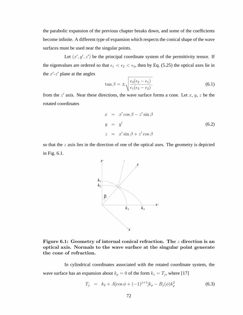
the parabolic expansion of the previous chapter breaks down, and some of the coefficients
become infinite. A different type of expansion which respects the conical shape of the wave
surfaces must be used near the singular points.
Let (x′, y′, z′) be the principal coordinate system of the permittivity tensor. If
the eigenvalues are ordered so thatε1 < ε2 < ε3, then by Eq. (5.25) the optical axes lie in
thex′-z′ plane at the angles
tan β = ±√√√√ε3(ε2 − ε1)
ε1(ε3 − ε2). (6.1)
from thez′ axis. Near these directions, the wave surface forms a cone. Letx, y, z be the
rotated coordinates
x = x′ cos β − z′ sin β
y = y′ (6.2)
z = x′ sin β + z′ cos β
so that thez axis lies in the direction of one of the optical axes. The geometry is depicted
in Fig. 6.1.
’
’
1
β
2
2 3
xkk
kk
zz
x
Figure 6.1: Geometry of internal conical refraction. The z direction is anoptical axis. Normals to the wave surface at the singular point generatethe cone of refraction.
In cylindrical coordinates associated with the rotated coordinate system, the
wave surface has an expansion aboutkρ = 0 of the formkz = Tj, where [17]
Tj = k2 + A[cos φ + (−1)j+1]kρ −Bj(φ)k2ρ (6.3)
72

Bj(φ) = B[1 + (−1)jD cos φ][1− (−1)jE cos φ]. (6.4)
Thej = 1 term corresponds to the external part of the wave surface andj = 2 to the inner
part. The constants are
A =1
2
√(ε3 − ε2)(ε2 − ε1)
ε1ε3
B =(ε3 + ε2)(ε2 + ε1)
8ε1ε3k02
D =ε3 − ε2
ε3 + ε2
E =ε2 − ε1
ε2 + ε1
wherek02 = ω√
ε2µ0. The apex angle of the cone of refraction is2A.
If we neglect the nonpropagating term, the tensor Green function for smallkρ is
given by Eq. (5.26) from the previous chapter,
G =2∑
j=1
ε2vjvj
k2z − T 2
j
(6.5)
where the polarization vectorsvj are expressed in the principal coordinate system. The
vectorsvj can be found from the electric flux density eigenvectors, which lie in the plane
perpendicular to thez axis. The vectorsDj corresponding to thevj are [64]
D1 = x cosφ
2+ y sin
φ
2
D2 = −x sinφ
2+ y cos
φ
2
whereφ is the azimuthal angle associated with the rotated coordinate system. Thevj are
proportional toε−1Dj, so that
v1′ = N
(x′ε−1
1 cos β cosφ
2+ y′ε−1
2 sinφ
2− z′ε−1
3 sin β cosφ
2
)(6.6)
with the normalization
N =
(ε−11 cos2 β cos2 φ
2+ ε−1
2 sin2 φ
2+ ε−1
3 sin2 β cos2 φ
2
)− 12
(6.7)
The eigenvectorv2 is equal tov1(φ + π).
73
The eigenvectorsvj can also be found from Eq. (5.7). The wavevectorkn =
(kρ cos φ, kρ sin φ, Tj) can be transformed into the principal coordinate system to yieldn′.
Thekj are given byk2j = k2
ρ + T 2j . Substituting these expressions into (5.7) and taking the
limit askρ goes to zero yields the result
vj′ = M
(x′
k02 sin β
k202 − k2
01
+ y′sin φ
2k02A(cos φ + (−1)j+1)+ z′
k02 cos β
k202 − k2
03
)(6.8)
whereM is a normalization such that (5.4) holds. Transforming to the unprimed coordinate
system,v1 can be shown to be parallel to
x cos (φ/2) + y sin (φ/2) + z2A cos (φ/2) (6.9)
andv2 to
−x sin (φ/2) + y cos (φ/2)− z2A sin (φ/2) (6.10)
which is equivalent to the result obtained in Ref. [67].
As in the previous chapter, I place an equivalent Gaussian surface currentJs =
ξ0p on thez = 0 plane at the waist of the beam, where
ξ0 =2E0
η2
e−ρ2/w20 δ(z) (6.11)
and the 1-formp specifies the polarization of the beam in the principal coordinate sys-
tem. The constantw0 specifies the waist size of the beam at its focus andη2 is the wave
impedance√
µ0/ε2. The beam is assumed to be focused at the incident face of the medium.
The electric field is then
E =iωµ0
8π3
∫dk eik·rG(k) ξ0(kρ)p (6.12)
whereξ0(kρ) = (2E0/η2)πw20e−w2
0k2ρ/4. Integratingkz by a contour closing in the upper
half plane yields forz > 0,
E = − k02
8π2ω
∫kρ dkρ dφeikρ(x cos φ+y sin φ)ξ0(kρ)
∑
j
vj(vj p)eiTjz (6.13)
where thevj are 1-forms dual to the vectorsvj. Substituting the expressions forξ0 andTj
given above yields
E = −k02w20E0e
ik02z
4πωη2
∫kρ dkρ dφ
∑
j
exp
[ikρ(g(φ) + (−1)j+1Az)− k2
ρ
(w2
0
4+ izBj
)]vj(vj p)
(6.14)
74
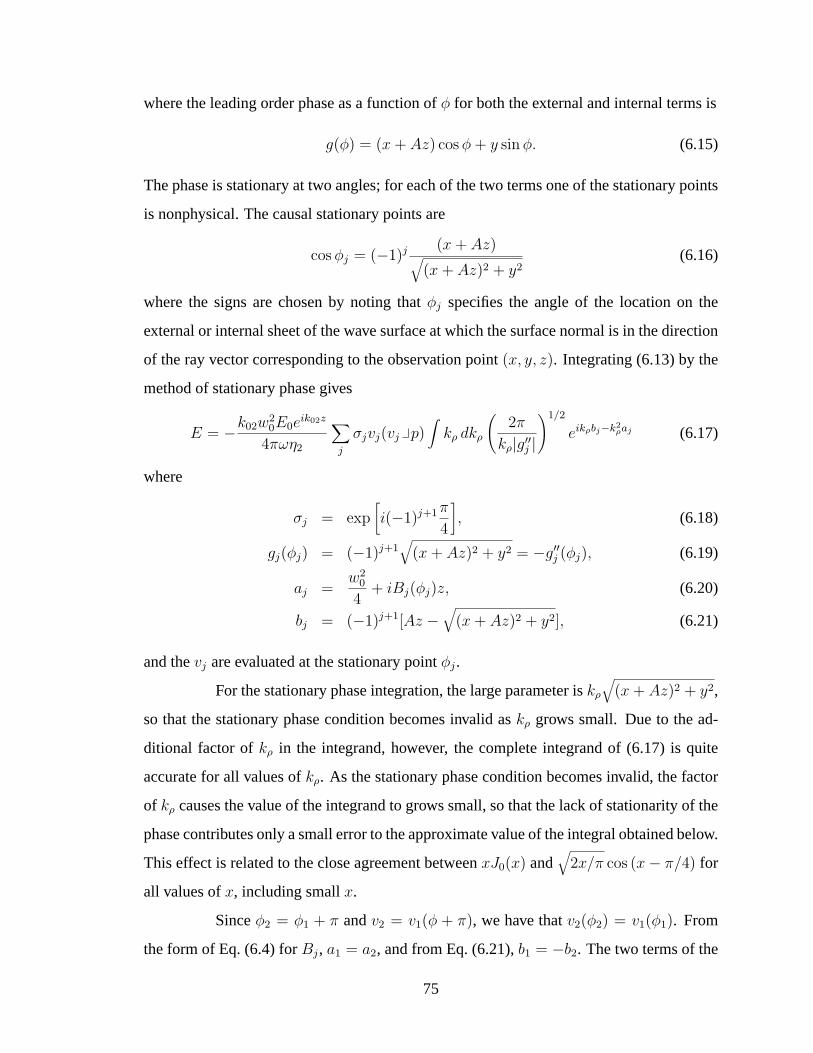
where the leading order phase as a function ofφ for both the external and internal terms is
g(φ) = (x + Az) cos φ + y sin φ. (6.15)
The phase is stationary at two angles; for each of the two terms one of the stationary points
is nonphysical. The causal stationary points are
cos φj = (−1)j (x + Az)√(x + Az)2 + y2
(6.16)
where the signs are chosen by noting thatφj specifies the angle of the location on the
external or internal sheet of the wave surface at which the surface normal is in the direction
of the ray vector corresponding to the observation point(x, y, z). Integrating (6.13) by the
method of stationary phase gives
E = −k02w20E0e
ik02z
4πωη2
∑
j
σjvj(vj p)∫
kρ dkρ
(2π
kρ|g′′j |
)1/2
eikρbj−k2ρaj (6.17)
where
σj = exp[i(−1)j+1π
4
], (6.18)
gj(φj) = (−1)j+1√
(x + Az)2 + y2 = −g′′j (φj), (6.19)
aj =w2
0
4+ iBj(φj)z, (6.20)
bj = (−1)j+1[Az −√
(x + Az)2 + y2], (6.21)
and thevj are evaluated at the stationary pointφj.
For the stationary phase integration, the large parameter iskρ
√(x + Az)2 + y2,
so that the stationary phase condition becomes invalid askρ grows small. Due to the ad-
ditional factor ofkρ in the integrand, however, the complete integrand of (6.17) is quite
accurate for all values ofkρ. As the stationary phase condition becomes invalid, the factor
of kρ causes the value of the integrand to grows small, so that the lack of stationarity of the
phase contributes only a small error to the approximate value of the integral obtained below.
This effect is related to the close agreement betweenxJ0(x) and√
2x/π cos (x− π/4) for
all values ofx, including smallx.
Sinceφ2 = φ1 + π andv2 = v1(φ + π), we have thatv2(φ2) = v1(φ1). From
the form of Eq. (6.4) forBj, a1 = a2, and from Eq. (6.21),b1 = −b2. The two terms of the
75

integral in (6.17) can then be combined, so that the electric field intensity becomes
E = −k02w20E0e
ik02z
4πωη2
v1(v1 p)
(2π
|g′′1 |
)1/2
eiπ/4∫ ∞
−∞
√kρ dkρe
ikρb1−k2ρa1 (6.22)
The remainingkρ integration can be evaluated exactly using the integral ([78], 3.462 #3)
∫ ∞
−∞
√xeibx−ax2
=√
πe−iπ/42−1/4a−3/4e−b2/(8a)D1/2
( −b√2a
)(6.23)
whereDν is the parabolic cylinder function. (A parabolic cylinder function of order1/2 has
also been obtained in connection with a different integral arising from conical refraction by
a gyrotropic medium in a certain limit [69].)
Asymptotically, the functionD1/2(x) depends exponentially on the square of
its argument. The expression (6.23) can be put into a more useful form in which this
asymptotic dependence is extracted and combined with the existing exponential factor of
e−b2/(8a). This is done using the relationship ([78], 9.240)
Dν(x) = 2ν/2e−x2/4
[ √π
Γ(1/4)1F1
(−ν
2,1
2,x2
2
)− x
√2π
Γ(−ν/2)1F1
(1− ν
2,3
2,x2
2
)](6.24)
for the parabolic cylinder function in terms of the hypergeometric function1F1 and the
expression ([78], 8.972 #1)
Lαn(x) =
Γ(n + α + 1)
Γ(n + 1)Γ(1− α)1F1(−n, α + 1, x) (6.25)
for the associated Laguerre functionLαn in terms of the hypergeometric function. These
relationships, along with the identitiesπ√
2 = Γ(1/4)Γ(3/4) = −Γ(−1/4)Γ(5/4), yield
the result
e−iπ/4
√2a3/4
e−b2/(4a)
[Γ(1/2)Γ(5/4)L
−1/21/4
(b2
4a
)− b√
aΓ(3/2)Γ(3/4)L
1/2−1/4
(b2
4a
)](6.26)
for the integral (6.23).
By using this result, the finalkρ integration of Eq. (6.22) can be performed, so
that the electric field intensity for the refracted Gaussian beam is
E = − ε2w20E0e
ik02z
4√
π[(x + Az)2 + y2]1/4a3/41
v1(φ1)[v1(φ1) p] F (a1, b1) (6.27)
76
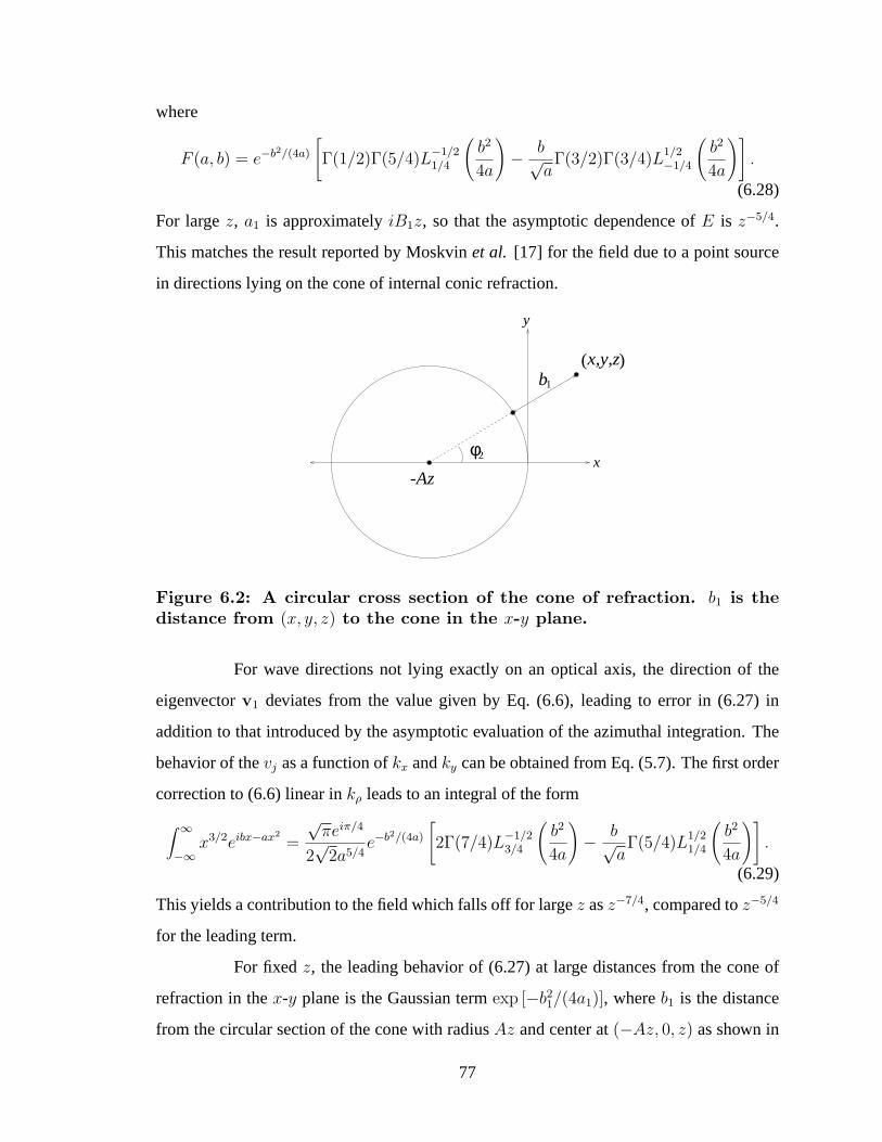
where
F (a, b) = e−b2/(4a)
[Γ(1/2)Γ(5/4)L
−1/21/4
(b2
4a
)− b√
aΓ(3/2)Γ(3/4)L
1/2−1/4
(b2
4a
)].
(6.28)
For largez, a1 is approximatelyiB1z, so that the asymptotic dependence ofE is z−5/4.
This matches the result reported by Moskvinet al. [17] for the field due to a point source
in directions lying on the cone of internal conic refraction.
b1
( )x,y,z
2
-Azx
y
φ
Figure 6.2: A circular cross section of the cone of refraction. b1 is thedistance from (x, y, z) to the cone in the x-y plane.
For wave directions not lying exactly on an optical axis, the direction of the
eigenvectorv1 deviates from the value given by Eq. (6.6), leading to error in (6.27) in
addition to that introduced by the asymptotic evaluation of the azimuthal integration. The
behavior of thevj as a function ofkx andky can be obtained from Eq. (5.7). The first order
correction to (6.6) linear inkρ leads to an integral of the form
∫ ∞
−∞x3/2eibx−ax2
=
√πeiπ/4
2√
2a5/4e−b2/(4a)
[2Γ(7/4)L
−1/23/4
(b2
4a
)− b√
aΓ(5/4)L
1/21/4
(b2
4a
)].
(6.29)
This yields a contribution to the field which falls off for largez asz−7/4, compared toz−5/4
for the leading term.
For fixedz, the leading behavior of (6.27) at large distances from the cone of
refraction in thex-y plane is the Gaussian termexp [−b21/(4a1)], whereb1 is the distance
from the circular section of the cone with radiusAz and center at(−Az, 0, z) as shown in
77
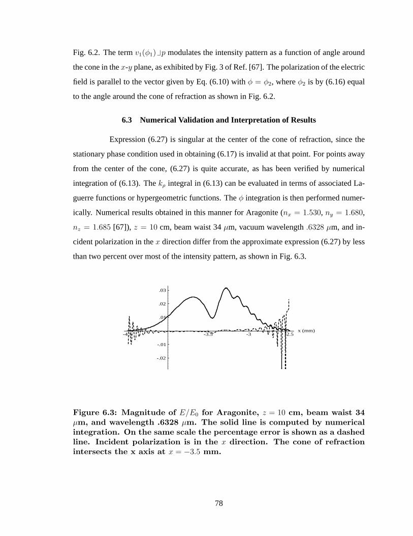
Fig. 6.2. The termv1(φ1) p modulates the intensity pattern as a function of angle around
the cone in thex-y plane, as exhibited by Fig. 3 of Ref. [67]. The polarization of the electric
field is parallel to the vector given by Eq. (6.10) withφ = φ2, whereφ2 is by (6.16) equal
to the angle around the cone of refraction as shown in Fig. 6.2.
6.3 Numerical Validation and Interpretation of Results
Expression (6.27) is singular at the center of the cone of refraction, since the
stationary phase condition used in obtaining (6.17) is invalid at that point. For points away
from the center of the cone, (6.27) is quite accurate, as has been verified by numerical
integration of (6.13). Thekρ integral in (6.13) can be evaluated in terms of associated La-
guerre functions or hypergeometric functions. Theφ integration is then performed numer-
ically. Numerical results obtained in this manner for Aragonite (nx = 1.530, ny = 1.680,
nz = 1.685 [67]), z = 10 cm, beam waist 34µm, vacuum wavelength.6328 µm, and in-
cident polarization in thex direction differ from the approximate expression (6.27) by less
than two percent over most of the intensity pattern, as shown in Fig. 6.3.
-4.5 -3.5 -3 -2.5x (mm)
-.02
-.01
.01
.02
.03
Figure 6.3: Magnitude of E/E0 for Aragonite, z = 10 cm, beam waist 34µm, and wavelength .6328 µm. The solid line is computed by numericalintegration. On the same scale the percentage error is shown as a dashedline. Incident polarization is in the x direction. The cone of refractionintersects the x axis at x = −3.5 mm.
78
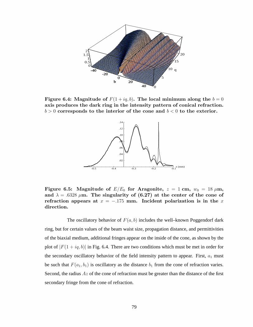
-40-20
020
40b
0
5
10
15
20
q0
0.51
1.52
-40-20
020
40b
Figure 6.4: Magnitude of F (1 + iq, b). The local minimum along the b = 0axis produces the dark ring in the intensity pattern of conical refraction.b > 0 corresponds to the interior of the cone and b < 0 to the exterior.
-0.5 -0.4 -0.3 -0.2 -0.1x (mm)
.02
.04
.06
.08
.10
.12
.14
Figure 6.5: Magnitude of E/E0 for Aragonite, z = 1 cm, w0 = 18 µm,and λ = .6328 µm. The singularity of (6.27) at the center of the cone ofrefraction appears at x = −.175 mm. Incident polarization is in the xdirection.
The oscillatory behavior ofF (a, b) includes the well–known Poggendorf dark
ring, but for certain values of the beam waist size, propagation distance, and permittivities
of the biaxial medium, additional fringes appear on the inside of the cone, as shown by the
plot of |F (1 + iq, b)| in Fig. 6.4. There are two conditions which must be met in order for
the secondary oscillatory behavior of the field intensity pattern to appear. First,a1 must
be such thatF (a1, b1) is oscillatory as the distanceb1 from the cone of refraction varies.
Second, the radiusAz of the cone of refraction must be greater than the distance of the first
secondary fringe from the cone of refraction.
79
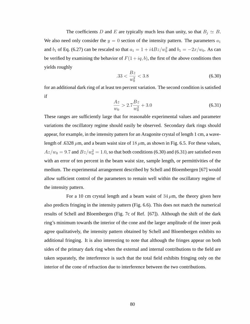
The coefficientsD andE are typically much less than unity, so thatBj ' B.
We also need only consider they = 0 section of the intensity pattern. The parametersa1
andb1 of Eq. (6.27) can be rescaled so thata1 = 1 + i4Bz/w20 andb1 = −2x/w0. As can
be verified by examining the behavior ofF (1 + iq, b), the first of the above conditions then
yields roughly
.33 <Bz
w20
< 3.8 (6.30)
for an additional dark ring of at least ten percent variation. The second condition is satisfied
ifAz
w0
> 2.7Bz
w20
+ 3.0 (6.31)
These ranges are sufficiently large that for reasonable experimental values and parameter
variations the oscillatory regime should easily be observed. Secondary dark rings should
appear, for example, in the intensity pattern for an Aragonite crystal of length 1 cm, a wave-
length of .6328µm, and a beam waist size of18 µm, as shown in Fig. 6.5. For these values,
Az/w0 = 9.7 andBz/w20 = 1.0, so that both conditions (6.30) and (6.31) are satisfied even
with an error of ten percent in the beam waist size, sample length, or permittivities of the
medium. The experimental arrangement described by Schell and Bloembergen [67] would
allow sufficient control of the parameters to remain well within the oscillatory regime of
the intensity pattern.
For a 10 cm crystal length and a beam waist of34 µm, the theory given here
also predicts fringing in the intensity pattern (Fig. 6.6). This does not match the numerical
results of Schell and Bloembergen (Fig. 7c of Ref. [67]). Although the shift of the dark
ring’s minimum towards the interior of the cone and the larger amplitude of the inner peak
agree qualitatively, the intensity pattern obtained by Schell and Bloembergen exhibits no
additional fringing. It is also interesting to note that although the fringes appear on both
sides of the primary dark ring when the external and internal contributions to the field are
taken separately, the interference is such that the total field exhibits fringing only on the
interior of the cone of refraction due to interference between the two contributions.
80
Figure 6.6: Same as Fig. 6.3, except that dashed lines are magnitudesof the internal and external contributions taken separately and the solidline is total intensity as given by Eq. (6.27).
81
6.4 Summary
The intensity pattern due to internal conical refraction of a narrow beam by
a biaxial medium apparently has a more complicated structure than previously thought,
since the theory given here predicts additional dark rings on the interior of the cone for
certain values of the material parameters, beam waist size, wavelength, and propagation
distance. The existence of the primary dark ring in the intensity pattern can be explained
heuristically, as is done in Ref. [7], by noting that if a narrow beam is considered to be a
sum of plane waves, the solid angle of the plane wave components reaching a thin circle
near the dark ring vanishes as the thin circle approaches the dark ring. For the secondary
dark rings, however, there is no such qualitative explanation.
For biaxial media, there apparently do not exist in the literature measurements
of the intensity pattern for beam and material parameters for which secondary dark rings
would be expected to appear. It seems desirable to further explore conical refraction exper-
imentally. I have given a reasonable sample size and beamwidth for Aragonite at which the
fringes should appear and indicated generally how beam and material parameters relate to
the appearance of oscillatory behavior in the intensity pattern.
82
Chapter 7
CONCLUSION
The purpose of this dissertation is to provide new techniques for analysis of
electromagnetic fields in anisotropic, inhomogeneous media. The primary results are a
new formalism for tensor Green functions for anisotropic media, an integral equation gen-
eralizing to anisotropic, inhomogeneous media the standard isotropic solution method in-
volving the Green function for the scalar Helmholtz equation, a new integral equation for
the electric field for complex media, closed form expressions for the Gaussian beam wave
solutions in biaxial media, and a precise analysis of internal conical refraction in biaxial
media predicting the appearance of secondary dark rings in the associated intensity pattern.
The electric field integral equation obtained in Chap. 3 and discussed in Chap.
4 is of interest for two classes of media. The first is that of a homogeneous medium, for
which the Helmholtz Green form can be obtained exactly. The integral equation then has
a closed–form kernel, and may be useful as a basis for numerical methods. The second
case is that of an isotropic, homogeneous medium, for which the Helmholtz Green form
reduces to the Green function for the scalar scattering by the same medium. To support
possible applications of this integral equation, I show how it reduces to standard results for
the isotropic, homogeneous special case, give principal value interpretations for the integral
involving highly singular derivatives of the Helmholtz Green form, and compare the equa-
tion to the usual integral equation method for electrically anisotropic and inhomogeneous
media.
Important physical problems involving propagation in anisotropic media can
be solved by a knowledge of the narrow beam solutions for the medium, including the
analysis of optical devices which rely on anisotropic media. Since a biaxial medium is
easier to analyze than more general media and is encountered commonly in applications,
for the study of beams I restrict study to this special type of medium. For an unbounded
biaxial medium, Chap. 5 gives the Gaussian beam solutions for all directions in the medium
except those which are near one of the optical axes. The phenomenon of internal conical
83
refraction of beams propagating along these singular directions has been analyzed before,
but the more precise analysis of Chap. 6 predicts a new effect, the existence of secondary
dark rings concentric to the well–known Poggendorf dark ring in the intensity pattern of
the refracted beam. I provide a numerical validations of the result and specify ranges of
material parameters which should be suitable for experimental verification of the effect.
In addition to the presentation of the results noted above, this dissertation is
intended to help establish the calculus of differential forms as a tool for applied electro-
magnetics problems. Results supporting this aim include the development of a geometrical
meaning for field quantities expressed as differential forms in Chap. 2 and Appendix B.
Appendix A gives the derivation of a new representation for electromagnetic boundary
conditions, which is shown in Chap. 2 to have a clear geometrical meaning. In Chap. 3,
the Hodge star operator is extended to allow its use for characterization of complex me-
dia with nonsymmetric permeability or permittivity tensors, and important theorems and
definitions such as that of the Laplace–de Rham operator are generalized to the case of a
nonsymmetric star operator. If one employs vectors and dyads, the derivation of key results
in this dissertation is hindered by the necessity of separately proving many special cases of
required identities. These results extend the utility of the calculus of differential forms as a
formalism for the development of new theoretical methods.
7.1 Further Research
It is hoped that new directions of research on the electromagnetics of complex
media will arise from this work, either through direct applications of the results presented
here or through new applications of the general approach and formalism for Green function
theory. There are a number of avenues for further work in extending the methods developed
in this dissertation. These include:
• Use of the electric field or Green form integral equation as a basis for numerical
methods of analyzing propagation in anisotropic, homogeneous media or isotropic,
inhomogeneous media for which the Helmholtz Green form can be represented ex-
actly;
84
• Determination of solutions for the Helmholtz Green form for bounded homogeneous
media of various shapes which satisfy specified boundary conditions;
• Determination of other exact solutions for the Helmholtz Green form; types of media
for which this may be possible include complex media with a certain symmetry,
such as an inhomogeneous, anisotropic medium with radially symmetric permittivity
profile;
• Investigation of the Helmholtz Green form and the associated derivative operator for
the case of a magnetically inhomogeneous medium;
• Further exploration of the Neumann series solution for the electric field, since there
may be types of media for which the series can be resummed in physical space or the
terms represented generally using special functions, leading to new field solutions
for the particular medium;
• Use of the integral equation for the case of an isotropic, electrically inhomogeneous
medium in seeking analytical, asymptotic or numerical results for electromagnetic
scattering from a knowledge of the scalar Green function, since the integral equation
links scalar scattering with full vector scattering for the same medium;
• Experimental verification of the secondary dark rings predicted by the results of
Chap. 6 for the intensity pattern of internal conical refraction, and a theoretical anal-
ysis of the relationship between the secondary fringes predicted by this theory and
those that appear in the intensity pattern for an optically active medium [6].
In addition, there are likely many unexplored applications of the calculus of differential
forms in applied electromagnetics other than the theory of Green functions. The strengths
of differential forms are most evident when one is deriving coordinate–free expressions,
rather than solving a problem for a specific source or boundary condition in a particular
coordinate system. This makes the calculus of differential forms ideal as a tool for seeking
new theoretical approaches. Differential forms also provide a link between electromagnet-
ics and a large body of pure mathematical theory, and methods from these fields might be
applied to the problems of applied electromagnetics. I hope that this work on the theory of
85

Green functions will provide not only numerical and analytical approaches to the solution
of problems involving electromagnetic propagation in complex media but also a foundation
for further theoretical developments in other areas of electromagnetics through the use of
the calculus of differential forms.
86
Bibliography
[1] K. F. Warnick, R. H. Selfridge, and D. V. Arnold, “Teaching electromagnetic field
theory using differential forms,”IEEE Trans. Educ., vol. 40, pp. 53–68, Feb. 1997.
[2] K. F. Warnick, R. H. Selfridge, and D. V. Arnold, “Electromagnetic boundary condi-
tions using differential forms,”IEE Proc., vol. 142, no. 4, pp. 326–332, 1995.
[3] K. F. Warnick and D. V. Arnold, “Electromagnetic Green functions using differential
forms,” J. Elect. Waves Appl., vol. 10, no. 3, pp. 427–438, 1996.
[4] K. F. Warnick and D. V. Arnold, “Green forms for anisotropic, inhomogeneous me-
dia,” J. Elect. Waves Appl., in press, 1997.
[5] K. F. Warnick and D. V. Arnold, “Secondary dark rings of internal conical refraction,”
Phys. Rev. E, in press, 1997.
[6] A. J. Schell and N. Bloembergen, “Laser studies of internal conical diffraction. II.
intensity patterns in an optically active crystal,α–iodic acid,”J. Opt. Soc. Am., vol. 68,
pp. 1098–1106, Aug. 1978.
[7] M. Born and E. Wolf,Principles of Optics. Oxford: Pergamon, 1980.
[8] L. D. Landau and E. M. Lifshitz,Electrodynamics of Continuous Media. New York:
Pergamon, 2 ed., 1984.
[9] P. Boulanger and M. Hayes, “Electromagnetic planes waves in anisotropic media: An
approach using bivectors,”Phil. Trans. R. Soc. Lond. A, vol. 330, pp. 335–393, 1990.
[10] N. Weck, “Maxwell’s boundary value problem on Riemannian manifolds with nons-
mooth boundaries,”J. Math. Anal. Appl., vol. 46, pp. 410–437, 1974.
[11] R. Picard, “Eigensolution expansions for generalized Maxwell fields on C0,1–
manifolds with boundary,”Applic. Anal., vol. 21, pp. 261–296, 1986.
[12] W. Thirring,Classical Field Theory, vol. II. New York: Springer-Verlag, 2 ed., 1978.
87
[13] P. Bamberg and S. Sternberg,A Course in Mathematics for Students of Physics, vol. II.
Cambridge: Cambridge University Press, 1988.
[14] W. S. Weiglhofer, “Dyadic Green’s functions for general uniaxial media,”IEE Proc.
H, vol. 137, pp. 5–10, Feb. 1990.
[15] D. I. Kaklamani and N. K. Uzunoglu, “Radiation of a dipole in an infinite triaxial
anisotropic medium,”Electromagnetics, vol. 12, pp. 231–245, 1992.
[16] M. Lax and D. F. Nelson, “Linear and nonlinear electrodynamics in elastic anisotropic
dielectrics,”Phys. Rev. B, vol. 4, pp. 3694–3731, 1971.
[17] D. N. Moskvin, V. P. Romanov, and A. Y. Val’kov, “Green’s function of the electro-
magnetic field in biaxial media,”Phys. Rev. E, vol. 48, no. 2, pp. 1436–1446, 1993.
[18] W. Ren, “Contributions to the electromagnetic wave theory of bounded homogenous
anisotropic media,”Phys. Rev. E, vol. 47, pp. 664–673, Jan. 1993.
[19] K. F. Warnick and M. A. Jensen, “The recursive Green function method for domain
decomposition,”Appl. Num. Math., In Review.
[20] A. Ben–Menahem, “Green’s tensors and associated potentials for electromagnetic
waves in inhomogeneous material media,”Proc. R. Soc. Lond. A, vol. 426, pp. 79–
106, 1989.
[21] G. de Rham,Differentiable Manifolds. New York: Springer-Verlag, 1984.
[22] H. Cartan,Differential Forms. Boston: Houghton Mifflin, 1970.
[23] C. Misner, K. Thorne, and J. A. Wheeler,Gravitation. San Francisco: Freeman, 1973.
[24] C. Nash and S. Sen,Topology and geometry for physicists. San Diego, California:
Academic Press, 1983.
[25] H. Flanders,Differential Forms with Applications to the Physical Sciences. New York,
New York: Dover, 1963.
88

[26] Y. Choquet-Bruhat and C. DeWitt-Morette,Analysis, Manifolds and Physics. Ams-
terdam: North-Holland, rev. ed., 1982.
[27] S. Hassani,Foundations of Mathematical Physics. Boston: Allyn and Bacon, 1991.
[28] R. Hermann,Topics in the geometric theory of linear systems. Brookline, MA: Math
Sci Press, 1984.
[29] Y. Choquet-Bruhat and C. DeWitt-Morette,Analysis, Manifolds and Physics. Part II:
92 Applications, vol. 2. Amsterdam: North-Holland, 1989.
[30] W. L. Burke, Applied Differential Geometry. Cambridge: Cambridge University
Press, 1985.
[31] R. S. Ingarden and A. Jamiołkowksi,Classical Electrodynamics. Amsterdam, The
Netherlands: Elsevier, 1985.
[32] S. Parrott,Relativistic Electrodynamics and Differential Geometry. New York:
Springer-Verlag, 1987.
[33] G. A. Deschamps, “Electromagnetics and differential forms,”IEEE Proc., vol. 69,
pp. 676–696, June 1981.
[34] D. Baldomir, “Differential forms and electromagnetism in 3-dimensional Euclidean
space R3,” IEE Proc., vol. 133, pp. 139–143, May 1986.
[35] N. Schleifer, “Differential forms as a basis for vector analysis—with applications to
electrodynamics,”Am. J. Phys., vol. 51, pp. 1139–1145, Dec. 1983.
[36] D. B. Nguyen, “Relativistic constitutive relations, differential forms, and the p-
compound,”Am. J. Phys., vol. 60, pp. 1137–1147, Dec. 1992.
[37] D. Baldomir and P. Hammond, “Global geometry of electromagnetic systems,”IEE
Proc., vol. 140, pp. 142–150, Mar. 1992.
89
[38] R. Mingzhong, T. Banding, and H. Jian, “Differential forms with applications to de-
scription and analysis of electromagnetic problems,”Proc. CSEE, vol. 14, pp. 56–62,
Sept. 1994.
[39] V. I. Karloukovski, “On the formulation of electrodynamics in terms of differential
forms,” Annuaire de l’Universite de Sofia Faculte de Physique, vol. 79, pp. 3–12,
1986.
[40] W. L. Engl, “Topology and geometry of the electromagnetic field,”Radio Sci., vol. 19,
pp. 1131–1138, Sept.–Oct. 1984.
[41] P. Hammond and D. Baldomir, “Dual energy methods in electromagnetics using tubes
and slices,”IEE Proc., vol. 135, pp. 167–172, Mar. 1988.
[42] A. Bossavit, “Differential forms and the computation of fields and forces in electro-
magnetism,”Eur. J. Mech. B, vol. 10, no. 5, pp. 474–488, 1991.
[43] I. Sasaki and T. Kasai, “Algebraic–topological interpretations for basic equations of
electromagnetic fields,”Bull. Univ. Osaka Prefecture A, vol. 25, no. 1-2, pp. 49–57,
1976.
[44] W. L. Burke, “Manifestly parity invariant electromagnetic theory and twisted tensors,”
J. Math. Phys., vol. 24, pp. 65–69, Jan. 1983.
[45] N. Salingaros, “Relativistic motion of a charged particle, the Lorentz group, and the
Thomas precession,”J. Math. Phys., vol. 25, pp. 706–716, Mar. 1984.
[46] N. Salingaros, “The gyrofrequency of a charged particle in a constant electromagnetic
field,” Il Nuovo Cimento, vol. 90 B, pp. 232–253, Dec. 1985.
[47] P. R. Kotiuga, “On making cuts for magnetic scalar potentials in multiply connected
regions,”J. Appl. Phys., vol. 61, pp. 3916–3918, Apr. 1987.
[48] P. R. Baldwin, “Constructing Clebsch potentials for vector fields,” Unpublished.
[49] P. R. Baldwin and R. M. Kiehn, “A classification result for linearly polarized principal
electromagnetic waves,”Phys. Lett. A, vol. 189, pp. 161–166, 1994.
90
[50] K. F. Warnick, D. V. Arnold, and R. H. Selfridge, “Electromagnetics made easy:
differential forms as a teaching tool,”Frontiers in Education Proceedings, Salt Lake
City, UT, 1996.
[51] J. A. Schouten,Pfaff ’s Problem and its Generalizations. New York: Chelsea, 1969.
[52] W. C. Chew,Waves and Fields in Inhomogenous Media. New York: IEEE Press,
1995.
[53] A. D. Yaghjian, “Electric dyadic Green’s functions in the source region,”Proc. IEEE,
vol. 68, no. 2, pp. 248–263, 1980.
[54] Y. L. Li, C. H. Liu, and S. J. Franke, “Three–dimensional Green’s function for
wave propagation in a linear inhomogeneous medium–the exact analytic solution,”
J. Acoust. Soc. Am., vol. 87, pp. 2285–2291, June 1990.
[55] Y. L. Li, “Exact analytic expressions of Green’s functions for wave propagation in
certain types of range–dependent inhomogeneous media,”J. Acoust. Soc. Am., vol. 96,
pp. 484–490, July 1994.
[56] L. B. Felsen and N. Marcuvitz,Radiation and Scattering of Waves. Piscataway, NJ:
IEEE Press, 1994.
[57] D. E. Livesay and K. Chen, “Electromagnetic fields induced inside arbitrarily shaped
biological bodies,”IEEE Trans. Micr. Th. Tech., vol. MTT-22, pp. 1273–1280, Dec.
1974.
[58] J. J. H. Wong, “Analysis of a three–dimensional arbitrarily shaped dielectric or biolog-
ical body inside a rectangular waveguide,”IEEE Trans. Micr. Th. Tech., vol. MTT-26,
pp. 457–462, July 1978.
[59] J. A. Kong,Electromagnetic Wave Theory. New York: John Wiley & Sons, 1990.
[60] J. Ctyroky, “On the propagation of wave beams in anisotropic media,”Opt. Acta,
vol. 22, no. 5, pp. 435–441, 1975.
91
[61] S. Y. Shin and L. B. Felsen, “Gaussian beam in anisotropic medium,”Applied Physics,
vol. 5, pp. 239–250, Dec. 1974.
[62] J. A. Fleck and M. D. Felt, “Beam propagation in uniaxial anisotropic media,”J. Opt.
Soc. Am., vol. 73, pp. 920–926, July 1983.
[63] H. Ermert, “Gaussian beams in anisotropic media,”Electron. Lett., vol. 6, no. 22,
pp. 720–721, 1970.
[64] D. L. Portigal and E. Burstein, “Internal conical refraction,”J. Opt. Soc. Am., vol. 59,
pp. 1567–1573, 1969.
[65] E. Lalor, “An analytical approach to the theory of internal conical refraction,”J. Math.
Phys., vol. 13, pp. 449–454, 1972.
[66] H. Juretschke,Crystal Physics: Macroscopic Physics of Anisotropic Solids. New
York: Benjamin, 1974.
[67] A. J. Schell and N. Bloembergen, “Laser studies of internal conical diffraction. I.
Quantitative comparison of experimental and theoretical conical intensity distribution
in aragonite,”J. Opt. Soc. Am., vol. 68, pp. 1093–1098, Aug. 1978.
[68] G. A. Uhlmann, “Light intensity distribution in conical refraction,”Comm. Pure Appl.
Math., vol. 25, pp. 69–80, 1982.
[69] Y. A. Brodskii, I. G. Kondratev, and M. A. Miller, “Electromagnetic beams in
anisotropic media. I.,”Radiophys. Quant. Elect., vol. 12, pp. 1047–1055, Sept. 1969.
[70] Y. A. Brodskii, I. G. Kondratev, and M. A. Miller, “Electromagnetic beams in
anisotropic media. II.,”Radiophys. Quant. Elect., vol. 15, pp. 447–453, April 1972.
[71] O. N. Naida, “Tangential conical refraction in a three-dimensionally inhomogenous
weakly anisotropic medium,”Sov. Phys.–JETP, vol. 50, pp. 239–245, Aug. 1979.
[72] A. M. Belskii, “Properties of light-wave propagation in weakly biaxial crystals,”Opt.
Spectrosc., vol. 55, pp. 776–779, Oct. 1983.
92

[73] A. M. Belskii and A. P. Khapalyuk, “Propagation of confined light beams along the
beam axes of biaxial crystals,”Opt. Spectrosc., vol. 44, pp. 312–315, March 1978.
[74] A. G. Khatkevich, “Internal conical refraction of light beams,”Opt. Spectrosc.,
vol. 46, pp. 282–284, March 1979.
[75] V. N. Alexandroff, “II. Les solutions des equations de maxwell dans le cas de refrac-
tion conique interne,”J. Optics, vol. 15, no. 4, pp. 219–228, 1984.
[76] A. M. Goncharenko, V. N. Belyi, S. N. Kurilkina, A. G. Khatkevich, and N. A. Khilo,
“Focusing and suppression of diffractive divergence in propagation of light beams in
the vicinity of the optical axes of biaxial gyrotropic crystals,”Opt. Spectrosc., vol. 78,
no. 5, pp. 787–791, 1995.
[77] J. P. Feve, B. Boulanger, and G. Marnier, “Experimental study of internal and external
conical refractions in KTP,”Opt. Commun., vol. 105, pp. 243–252, 1994.
[78] I. S. Gradshteyn and I. M. Ryzhik,Table of Integrals, Series, and Products. San
Diego: Academic Press, 5 ed., 1994.
93
Appendix A
BOUNDARY CONDITIONS USING DIFFERENTIAL FORMS
In this appendix I derive a new formulation for the boundary conditions at a
discontinuity in the electromagnetic field using differential forms [2]. Thirring [12] and
Burke [30, 44] treat boundary conditions using the calculus of differential forms. Thirring’s
approach is similar to that given here, but his expressions for boundary sources include a
singularity in the direction normal to the boundary. The formulation given here is more
closely analogous to the usual vector boundary conditions than those given by Burke and
Thirring. As discussed in Sec. 2.4.5, the boundary conditions derived in this appendix have
intuitive geometric interpretations.
A.1 Derivation
In this section I derive an expression for sources on a boundary where a field
is discontinuous. The boundary condition associated with a general field equation can be
given in convenient form using an operator which projects a form to its component with
surfaces orthogonal to the boundary. The specializations to magnetic field intensity and
electric flux density are discussed further in Chap. 2.
A.1.1 Representing Surfaces With 1-forms
If the continuous and differentiable functionf(x1, ..., xn) vanishes (or is con-
stant) along a boundary, then when interpreted graphically the 1-formdf has a surface that
lies on the boundary. This 1-form can be used to express boundary conditions for fields
near a boundary. The surface of a paraboloid reflector antenna, for example, is given by
−x2−y2 +az = 0, so that the unnormalized boundary 1-form is−2x dx−2y dy+a dz. A
rough surface can be described by−h(x, y)+z = 0, giving the boundary 1-form−dh+ dz.
For the remainder of this appendix I will use the notation
n =df
|df | =df√
df df(A.1)
94
where is the interior product. The 1-formn is dual to the usual surface normal vectorn.
A.1.2 The Boundary Projection Operator
In this section, I derive a general expression for the boundary conditions satis-
fied by a field which is related to a source and another nonsingular field by exterior dif-
ferentiation. Letα be ap-form with p < n (wheren is the dimension of space) which
represents a field with a(p + 1)-form β as a source, so that
dα = γ + β (A.2)
whereγ is nonsingular. Letf = 0 represent a boundary, wheref is differentiable and
vanishes only along the boundary. Letα equalα1 for f > 0 andα2 for f < 0.
We can writeα = (α1 − α2)θ(f) + α2, whereθ is the unit step function. Then
γ + β = d(α1 − α2)θ(f) + α2= δ(f)df ∧ (α1 − α2) + θ(f)d(α1 − α2) + dα2. (A.3)
= δ(f)n ∧ (α1 − α2) + θ(f)d(α1 − α2) + dα2
whereδ is the Dirac delta function andδ(f) is δ(x1 − x10) · · · δ(xn − xn
0 ) such that the
point (x10, ..., x
n0 ) lies on the boundary andδ(f) = δ(f)/
√df df . The singular parts of
both sides of (A.3) must be equal, so that
β′ = δ(f)n ∧ (α1 − α2) (A.4)
whereβ′ is the singular part ofβ, representing the boundary source alongf = 0. Since the
sourceβ′ is confined to the boundary, it can be written [12]
β′ = δ(f)n ∧ βs (A.5)
whereβs is ap-form, the restriction ofβ′ to the boundary. Integrating (A.4) and (A.5) over
a small region containing the boundary shows that the equality
n ∧ βs = n ∧ (α1 − α2). (A.6)
95

must hold on the boundary. The interior product distributes over the exterior product ac-
cording to the relationship
α (β ∧ γ) = (α β) ∧ γ + (−1)pβ ∧ (α γ) (A.7)
wherep is the degree ofβ andα is a 1-form. Taking the interior product of both sides of
(A.6) with n and applying the identity (A.7) yields
n (n ∧ (α1 − α2)) = n (n ∧ βs)
= (n n) ∧ βs − n ∧ (n βs). (A.8)
By definition, we have thatn n = 1. Since the sourceβs is confined to the boundary,
n βs = 0. By interpreting this graphically, we see that the surfaces ofβs must be perpen-
dicular to the boundary, so thatβs can contain no factor ofn. Applying this to (A.8), we
have
βs = n (n ∧ (α1 − α2)) (A.9)
which is the central result of this appendix. Note that the source may be represented by a
twisted form, as defined and discussed in detail in Ref. [2]. In this case, an orientation for
βs must be specified. In practice, the distinction between twisted and nontwisted forms can
be ignored and the sense of the current or charge represented byβs obtained precisely in a
straighforward manner, as explained in the following section.
The operatorn n∧ can be interpreted as a boundary projection operator. Ge-
ometrically, its action on a differential form is to remove the component of the form with
surfaces parallel to the boundary. The boundary projection of a 1-form has surfaces per-
pendicular to the boundary. The boundary projection of a 2-form has tubes perpendicular
to the surface at every point.
Since the boundary condition derived above applies to any law of the form of
Eq. (A.2), Maxwell’s laws (2.4) lead to
n (n ∧ (E1 − E2)) = 0
n (n ∧ (H1 −H2)) = Js
n (n ∧ (D1 −D2)) = ρs (A.10)
n (n ∧ (B1 −B2)) = 0
96
whereJs is the surface current 1-form andρs is the surface charge 2-form. In four-space
we havedF = 0 anddG = j, whereF = B+E∧ dt, G = D−H∧ dt andj = ρ−J∧ dt.
All four boundary conditions can be expressed as
n (n ∧ (F1 − F2)) = 0
n (n ∧ (G1 −G2)) = js (A.11)
wherejs = ρs − Js ∧ dt.
A.1.3 Orientation of Sources
The direction of flow of the surface current represented byJs and the sign of
the surface charge represented byρs cannot be obtained directly from the formsJs andρs
alone. If the labels 1 and 2 of the two sides of a boundary are interchanged, the signs ofJs
andρs also change. The signs of the vector surface current densityJs and the scalar charge
densityqs do not change. If the quantitiesJs or qs are integrated to yield total current or
charge, however, one must choose a differential path length or differential surface element.
There are two possible signs for these differential elements. This additional sign is already
present in the differential formsJs andρs.
Although the sign change with respect to the labeling of regions makes the sense
of the sources represented byJs andρs more difficult to specify precisely than is the case
with the vector boundary sources, the differential forms lead to simpler integral expressions
for total current and charge. For many electromagnetic quantities, the vector representation
and the representation as a differential form are duals, so that their components differ only
by metrical coefficients. This is not the case for the surface current and charge density
forms yielded by the boundary projection operator. The integral of the surface current
densityJs over a path should yield the total current through the path. The 1-formJs as
obtained using the boundary projection operator satisfies this definition:
I =∫
PJs (A.12)
whereP is a path. The sense ofI is with respect to the direction of the 2-formn ∧ s,
wheres is the 1-form dual to the tangent vectors of P (so thats is a 1-form with surfaces
97
perpendicular to the pathP and oriented in the direction of integration). The total current
given by (2.6) in terms of the vector surface current density is less natural than (A.12).
The total charge on an areaA of a boundary with surface chargeρs is
Q =∫
Aρs. (A.13)
In order to obtain the proper sign forQ, the orientation ofA must be such that a 2-form
ω which satisfiesn ∧ ω = Ω also satisfies∫A ω > 0, whereΩ is the standard volume
element,dx dy dz in rectangular coordinates. The sign of the charge represented byρs can
also be found by computing(n ∧ ρs)/Ω. This complication in specifying the sense ofQ is
actually present when dealing with the scalar surface charge densityqs as well, since one
must choose the area elementdS and orientation ofA in Q =∫A qsdS such that
∫A dS is
positive in order to obtain the correct total charge.
A.2 Boundary Decomposition of Forms
The boundary conditions of the previous section appear to depend on a metric,
since the metric–dependent interior product of differential forms is employed. The bound-
ary projection operatorn n∧, however, is in a sense extraneous. The 1-formH1−H2, for
example, yields the same result as the surface currentJs = n (n∧ (H1−H2)) for integra-
tion over any path lying in the boundary. The formsJs andH1 −H2 are equivalent in that
they have the same restriction to the boundary. The boundary projection operator simply
removes the component of the form with surfaces parallel to the boundary with respect to
the metric. The metric has no effect on the relationship between the field discontinuity and
boundary source.
A metric independent type of boundary decomposition can be defined. Letf be
a function vanishing along a boundary as above. Letv be a an arbitrary vector field. The
interior product expands across the exterior product according to
v (α ∧ ω) = (v α) ∧ ω + (−1)pα ∧ (v ω) (A.14)
wherep is the degree ofα. Recall that the interior product of a vector and a form represents
the contraction of the vector with the leftmost index of the form, and is metric independent.
98
If α = df , then by rearranging (A.14) we have
(v df)ω = v (df ∧ ω) + df ∧ (v ω). (A.15)
Since the termdf ∧ (v ω) contains a factor ofdf , its integral over any region lying in the
boundaryf = 0 must vanish, as can be verified by integration by parts. The interior product
of v with the termv (df ∧ ω) vanishes by the antisymmetry of the tensordf ∧ ω. Thus,
Eq. (A.15) decomposes(v df)ω into two parts, one which has zero contraction withv and
another which integrates to zero over any region confined to the boundary. Furthermore, if
the vectorv is chosen such thatv df = 1, thenv df∧ anddf ∧v are both projections.
If the vectorv is related todf by a metric, then the termv (df ∧ω) is orthogo-
nal to the boundaryf = 0 in a metrical sense. In the previous section, the use ofn instead
of v is equivalent to obtainingv from df/|df | by raising its index using a metric.
If the boundary is sufficiently smooth, then there is a local coordinate system
x1, . . . , xn for which f = x1. If the vectorv is chosen to bex1 (or ∂x1 in the notation
of differential geometry), then the first term of the decomposition (A.15) consists of all
terms ofω which do not contain a factor ofdx1. This part ofω is the restriction ofω
to the boundary, since it is equal to the pullback ofω to the boundary by the function
(0, x2, . . . , xn). The second term of the decomposition includes the remaining terms ofω
which contain a factor ofdx1.
It is interesting to compare Eq. (A.15) to the definition of the wave operator∆.
For a constant metric the definition of the Laplace–de Rham operator can be written as [3]
(d d)ω = d (d ∧ ω) + d ∧ (d ω) (A.16)
where the interior product of the exterior derivative with another quantity is defined by
using the metric formally to convert the operatord = ∂/∂x1 dx1 + · · ·+ ∂/∂xn dxn from a
1-form to a vector and then contracting this vector with the first index of the second factor
of the interior product. The spatial Fourier transform of (A.16) is identical to (A.15) with
v equal to the wavevectork anddf replaced with the dual 1-formk.
Finally, I note that Burke’s formulation of boundary conditions provide an ele-
gant alternative proof of the result (A.9) [30]. In integral form, Eq. (A.2) is∮
∂Mα =
∫
Mγ +
∫
Mβ (A.17)
99
As the regionM approachesM ∩ B, whereB is the boundaryf = 0, the right–hand side
approaches ∫
Mγ +
∫
Mβ =
∫
M∩Bβs (A.18)
where theγ term drops out sinceγ is nonsingular and so its integral vanishes asM loses its
dimension in the direction perpendicular toB. In the same limit, the left–hand side reduces
to ∮
∂Mα =
∫
∂M1
α +∫
∂M2
α (A.19)
whereM1 is the part ofM on thef < 0 side of the boundary andM2 is the part on the
f > 0 side. This in turn becomes
∫
∂M1
α +∫
∂M2
α =∫
M∩B(p∗1α + p∗2α) (A.20)
wherep1 is a mapping from thef > 0 side of the boundary to the boundary,p2 is a mapping
from thef < 0 side of the boundary to the boundary, and the superscript∗ represents the
pullback operation. The integrand on the right is given the symbol[α] by Burke. By
combining Eqs. (A.18) and (A.20), we have that
∫
M∩B[α] =
∫
M∩Bβs (A.21)
SinceM can be chosen to be arbitrarily small, the integrands on both sides of this expres-
sion must be equal ifα andβs are sufficiently regular. The boundary condition onα can
thus be written
[α] = βs. (A.22)
By the above discussion, the pullback ofv (df ∧ α) to the boundary is equivalent to[α].
Furthermore, in a coordinate systemx1, . . . , xn such thatf = x1, then ifv = x1, the form
v (df ∧ α) is equal to[α] expressed in the same coordinate system.
100
Appendix B
TEACHING ELECTROMAGNETIC FIELD THEORY USING
DIFFERENTIAL FORMS
The material in this appendix is taken from Ref. [1]. It includes an elementary
introduction to electromagnetic field theory using differential forms, simple computational
examples, and a summary of the pedagogical advantages of differential forms. The primary
contribution of this appendix is to extend the geometric viewpoint advanced in Refs. [23]
and [30], providing a new viewpoint on the quantities and physical principles of electro-
magnetic field theory. This viewpoint is a valuable tool in both teaching and research.
B.1 Introduction
Certain questions are often asked by students of electromagnetic (EM) field the-
ory: Why does one need both field intensity and flux density to describe a single field? How
does one visualize the curl operation? Is there some way to make Ampere’s law or Fara-
day’s law as physically intuitive as Gauss’s law? The Stokes theorem and the divergence
theorem seem vaguely similar; do they have a deeper connection? Because of difficulty
with concepts related to these questions, some students leave introductory courses lack-
ing a real understanding of the physics of electromagnetics. Interestingly, none of these
concepts are intrinsically more difficult than other aspects of EM theory; rather, they are
unclear because of the limitations of the mathematical language traditionally used to teach
electromagnetics: vector analysis. In this appendix, we show that the calculus of differen-
tial forms clarifies these and other fundamental principles of electromagnetic field theory.
The use of the calculus of differential forms in electromagnetics has been ex-
plored in several important papers and texts, including Misner, Thorne, and Wheeler [23],
Deschamps [33], and Burke [30]. These works note some of the advantages of the use of
differential forms in EM theory. Misneret al. and Burke treat the graphical representation
of forms and operations on forms, as well as other aspects of the application of forms to
101
electromagnetics. Deschamps was among the first to advocate the use of forms in teaching
engineering electromagnetics.
Existing treatments of differential forms in EM theory either target an advanced
audience or are not intended to provide a complete exposition of the pedagogical advan-
tages of differential forms. This appendix presents the topic on an undergraduate level and
emphasizes the benefits of differential forms in teaching introductory electromagnetics,
especially graphical representations of forms and operators. The calculus of differential
forms and principles of EM theory are introduced in parallel, much as would be done in a
beginning EM course. We present concrete visual pictures of the various field quantities,
Maxwell’s laws, and boundary conditions. The aim of this appendix is to demonstrate that
differential forms are an attractive and viable alternative to vector analysis as a tool for
teaching electromagnetic field theory.
B.1.1 Development of Differential Forms
Cartan and others developed the calculus of differential forms in the early 1900’s.
A differential form is a quantity that can be integrated, including differentials. More pre-
cisely, a differential form is a fully covariant, fully antisymmetric tensor. The calculus of
differential forms is a self–contained subset of tensor analysis.
Since Cartan’s time, the use of forms has spread to many fields of pure and ap-
plied mathematics, from differential topology to the theory of differential equations. Dif-
ferential forms are used by physicists in general relativity [23], quantum field theory [24],
thermodynamics [13], mechanics [25], as well as electromagnetics. A section on differen-
tial forms is commonplace in mathematical physics texts [26, 27]. Differential forms have
been applied to control theory by Hermann [28] and others.
B.1.2 Differential Forms in EM Theory
The laws of electromagnetic field theory as expressed by James Clerk Maxwell
in the mid 1800’s required dozens of equations. Vector analysis offered a more convenient
tool for working with EM theory than earlier methods. Tensor analysis is in turn more
concise and general, but is too abstract to give students a conceptual understanding of EM
102
theory. Weyl and Poincare expressed Maxwell’s laws using differential forms early this
century. Applied to electromagnetics, differential forms combine much of the generality of
tensors with the simplicity and concreteness of vectors.
General treatments of differential forms and EM theory include papers [33],
[34], [35], [36], [37], and [41]. Ingarden and Jamiołkowksi [31] is an electrodynamics text
using a mix of vectors and differential forms. Parrott [32] employs differential forms to
treat advanced electrodynamics. Thirring [12] is a classical field theory text that includes
certain applied topics such as waveguides. Bamberg and Sternberg [13] develop a range
of topics in mathematical physics, including EM theory via a discussion of discrete forms
and circuit theory. Burke [30] treats a range of physics topics using forms, shows how
to graphically represent forms, and gives a useful discussion of twisted differential forms.
The general relativity text by Misner, Thorne and Wheeler [23] has several chapters on EM
theory and differential forms, emphasizing the graphical representation of forms. Flanders
[25] treats the calculus of forms and various applications, briefly mentioning electromag-
netics.
We note here that many authors, including most of those referenced above, give
the spacetime formulation of Maxwell’s laws using forms, in which time is included as a
differential. We use only the (3+1) representation in this appendix, since the spacetime
representation is treated in many references and is not as convenient for various elemen-
tary and applied topics. Other formalisms for EM theory are available, including bivectors,
quaternions, spinors, and higher Clifford algebras. None of these offer the combination
of concrete graphical representations, ease of presentation, and close relationship to tradi-
tional vector methods that the calculus of differential forms brings to undergraduate–level
electromagnetics.
The tools of applied electromagnetics have begun to be reformulated using dif-
ferential forms. The authors have developed a convenient representation of electromag-
netic boundary conditions [2]. Thirring [12] treats several applications of EM theory using
forms, and this dissertation applies differential forms to the Green function theory of com-
plex media.
103

B.1.3 Pedagogical Advantages of Differential Forms
As a language for teaching electromagnetics, differential forms offer several
important advantages over vector analysis. Vector analysis allows only two types of quan-
tities: scalar fields and vector fields (ignoring inversion properties). In a three–dimensional
space, differential forms of four different types are available. This allows flux density and
field intensity to have distinct mathematical expressions and graphical representations, pro-
viding the student with mental pictures that clearly reveal the different properties of each
type of quantity. The physical interpretation of a vector field is often implicitly contained
in the choice of operator or integral that acts on it. With differential forms, these properties
are directly evident in the type of form used to represent the quantity.
The basic derivative operators of vector analysis are the gradient, curl and diver-
gence. The gradient and divergence lend themselves readily to geometric interpretation, but
the curl operation is more difficult to visualize. The gradient, curl and divergence become
special cases of a single operator, the exterior derivative and the curl obtains a graphical
representation that is as clear as that for the divergence. The physical meanings of the curl
operation and the integral expressions of Faraday’s and Ampere’s laws become so intuitive
that the usual order of development can be reversed by introducing Faraday’s and Ampere’s
laws to students first and using these to motivate Gauss’s laws.
The Stokes theorem and the divergence theorem have an obvious connection in
that they relate integrals over a boundary to integrals over the region inside the boundary,
but in the language of vector analysis they appear very different. These theorems are special
cases of the generalized Stokes theorem for differential forms, which also has a simple
graphical interpretation.
Since 1992, in the Brigham Young University Department of Electrical and
Computer Engineering we have incorporated short segments on differential forms into our
beginning, intermediate, and graduate electromagnetics courses. In the Fall of 1995, we
reworked the entire beginning electromagnetics course, changing emphasis from vector
analysis to differential forms. Following the first semester in which the new curriculum
was used, students completed a detailed written evaluation. Out of 44 responses, four were
partially negative; the rest were in favor of the change to differential forms. Certainly,
104
enthusiasm of students involved in something new increased the likelihood of positive re-
sponses, but one fact was clear: pictures of differential forms helped students understand
the principles of electromagnetics.
B.1.4 Outline
Section B.2 defines differential forms and the degree of a form. Graphical rep-
resentations for forms of each degree are given, and the differential forms representing the
various quantities of electromagnetics are identified. In Sec. B.3 we use these differen-
tial forms to express Maxwell’s laws in integral form and give graphical interpretations
for each of the laws. Section B.4 introduces differential forms in curvilinear coordinate
systems. Section B.5 applies Maxwell’s laws to find the fields due to sources of basic
geometries. In Sec. B.6 we define the exterior derivative, give the generalized Stokes the-
orem, and express Maxwell’s laws in point form. Section B.7 treats boundary conditions
using the interior product. Section B.8 provides a summary of the main points made in the
appendix.
B.2 Differential Forms and the Electromagnetic Field
In this section we define differential forms of various degrees and identify them
with field intensity, flux density, current density, charge density and scalar potential.
A differential form is a quantity that can be integrated, including differentials.
3x dx is a differential form, as arex2y dx dy andf(x, y, z) dy dz + g(x, y, z) dz dx. The
type of integral called for by a differential form determines its degree. The form3x dx is
integrated under a single integral over a path and so is a 1-form. The formx2y dx dy is
integrated by a double integral over a surface, so its degree is two. A 3-form is integrated
by a triple integral over a volume. 0-forms are functions, “integrated” by evaluation at a
point. Table B.1 gives examples of forms of various degrees. The coefficients of the forms
can be functions of position, time, and other variables.
105
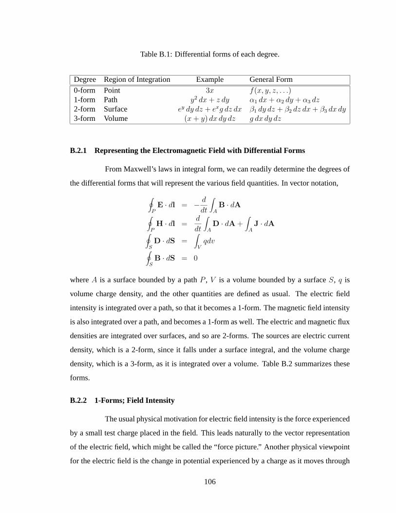
Table B.1: Differential forms of each degree.
Degree Region of Integration Example General Form
0-form Point 3x f(x, y, z, . . .)1-form Path y2 dx + z dy α1 dx + α2 dy + α3 dz2-form Surface ey dy dz + exg dz dx β1 dy dz + β2 dz dx + β3 dx dy3-form Volume (x + y) dx dy dz g dx dy dz
B.2.1 Representing the Electromagnetic Field with Differential Forms
From Maxwell’s laws in integral form, we can readily determine the degrees of
the differential forms that will represent the various field quantities. In vector notation,
∮
PE · dl = − d
dt
∫
AB · dA
∮
PH · dl =
d
dt
∫
AD · dA +
∫
AJ · dA
∮
SD · dS =
∫
Vqdv
∮
SB · dS = 0
whereA is a surface bounded by a pathP , V is a volume bounded by a surfaceS, q is
volume charge density, and the other quantities are defined as usual. The electric field
intensity is integrated over a path, so that it becomes a 1-form. The magnetic field intensity
is also integrated over a path, and becomes a 1-form as well. The electric and magnetic flux
densities are integrated over surfaces, and so are 2-forms. The sources are electric current
density, which is a 2-form, since it falls under a surface integral, and the volume charge
density, which is a 3-form, as it is integrated over a volume. Table B.2 summarizes these
forms.
B.2.2 1-Forms; Field Intensity
The usual physical motivation for electric field intensity is the force experienced
by a small test charge placed in the field. This leads naturally to the vector representation
of the electric field, which might be called the “force picture.” Another physical viewpoint
for the electric field is the change in potential experienced by a charge as it moves through
106
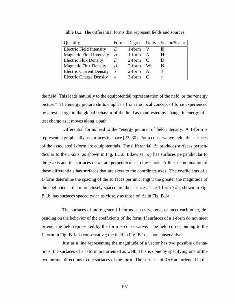
Table B.2: The differential forms that represent fields and sources.
Quantity Form Degree Units Vector/Scalar
Electric Field Intensity E 1-form V EMagnetic Field Intensity H 1-form A HElectric Flux Density D 2-form C DMagnetic Flux Density B 2-form Wb BElectric Current Density J 2-form A JElectric Charge Density ρ 3-form C q
the field. This leads naturally to the equipotential representation of the field, or the “energy
picture.” The energy picture shifts emphasis from the local concept of force experienced
by a test charge to the global behavior of the field as manifested by change in energy of a
test charge as it moves along a path.
Differential forms lead to the “energy picture” of field intensity. A 1-form is
represented graphically as surfaces in space [23, 30]. For a conservative field, the surfaces
of the associated 1-form are equipotentials. The differentialdx produces surfaces perpen-
dicular to thex-axis, as shown in Fig. B.1a. Likewise,dy has surfaces perpendicular to
they-axis and the surfaces ofdz are perpendicular to thez axis. A linear combination of
these differentials has surfaces that are skew to the coordinate axes. The coefficients of a
1-form determine the spacing of the surfaces per unit length; the greater the magnitude of
the coefficients, the more closely spaced are the surfaces. The 1-form2 dz, shown in Fig.
B.1b, has surfaces spaced twice as closely as those ofdx in Fig. B.1a.
The surfaces of more general 1-forms can curve, end, or meet each other, de-
pending on the behavior of the coefficients of the form. If surfaces of a 1-form do not meet
or end, the field represented by the form is conservative. The field corresponding to the
1-form in Fig. B.1a is conservative; the field in Fig. B.1c is nonconservative.
Just as a line representing the magnitude of a vector has two possible orienta-
tions, the surfaces of a 1-form are oriented as well. This is done by specifying one of the
two normal directions to the surfaces of the form. The surfaces of3 dx are oriented in the
107
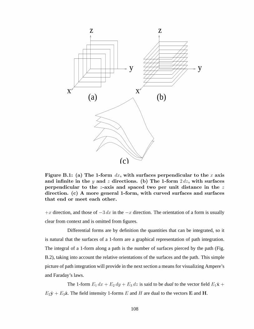
z
(a) (b)
(c)
x
z
y
x
y
Figure B.1: (a) The 1-form dx, with surfaces perpendicular to the x axisand infinite in the y and z directions. (b) The 1-form 2 dz, with surfacesperpendicular to the z-axis and spaced two per unit distance in the zdirection. (c) A more general 1-form, with curved surfaces and surfacesthat end or meet each other.
+x direction, and those of−3 dx in the−x direction. The orientation of a form is usually
clear from context and is omitted from figures.
Differential forms are by definition the quantities that can be integrated, so it
is natural that the surfaces of a 1-form are a graphical representation of path integration.
The integral of a 1-form along a path is the number of surfaces pierced by the path (Fig.
B.2), taking into account the relative orientations of the surfaces and the path. This simple
picture of path integration will provide in the next section a means for visualizing Ampere’s
and Faraday’s laws.
The 1-formE1 dx + E2 dy + E3 dz is said to bedual to the vector fieldE1x +
E2y + E3z. The field intensity 1-formsE andH are dual to the vectorsE andH.
108

Figure B.2: A path piercing four surfaces of a 1-form. The integral ofthe 1-form over the path is four.
Following Deschamps, we take the units of the electric and magnetic field inten-
sity 1-forms to be Volts and Amps, as shown in Table B.2. The differentials are considered
to have units of length. Other field and source quantities are assigned units according to
this same convention. A disadvantage of Deschamps’ system is that it implies in a sense
that the metric of space carries units. Alternative conventions are available; Bamberg and
Sternberg [13] and others take the units of the electric and magnetic field intensity 1-forms
to be V/m and A/m, the same as their vector counterparts, so that the differentials carry
no units and the integration process itself is considered to provide a factor of length. If
this convention is chosen, the basis differentials of curvilinear coordinate systems (see Sec.
B.4) must also be taken to carry no units. This leads to confusion for students, since these
basis differentials can include factors of distance. The advantages of this alternative con-
vention are that it is more consistent with the mathematical point of view, in which basis
vectors and forms are abstract objects not associated with a particular system of units, and
that a field quantity has the same units whether represented by a vector or a differential
form. Furthermore, a general differential form may include differentials of functions that
do not represent position and so cannot be assigned units of length. The possibility of con-
fusion when using curvilinear coordinates seems to outweigh these considerations, and so
we have chosen Deschamps’ convention.
109
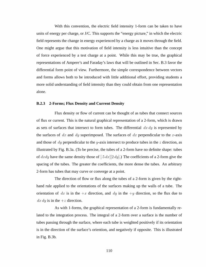
With this convention, the electric field intensity 1-form can be taken to have
units of energy per charge, or J/C. This supports the “energy picture,” in which the electric
field represents the change in energy experienced by a charge as it moves through the field.
One might argue that this motivation of field intensity is less intuitive than the concept
of force experienced by a test charge at a point. While this may be true, the graphical
representations of Ampere’s and Faraday’s laws that will be outlined in Sec. B.3 favor the
differential form point of view. Furthermore, the simple correspondence between vectors
and forms allows both to be introduced with little additional effort, providing students a
more solid understanding of field intensity than they could obtain from one representation
alone.
B.2.3 2-Forms; Flux Density and Current Density
Flux density or flow of current can be thought of as tubes that connect sources
of flux or current. This is the natural graphical representation of a 2-form, which is drawn
as sets of surfaces that intersect to form tubes. The differentialdx dy is represented by
the surfaces ofdx and dy superimposed. The surfaces ofdx perpendicular to thex-axis
and those ofdy perpendicular to they-axis intersect to produce tubes in thez direction, as
illustrated by Fig. B.3a. (To be precise, the tubes of a 2-form have no definite shape: tubes
of dxdy have the same density those of[.5 dx][2 dy].) The coefficients of a 2-form give the
spacing of the tubes. The greater the coefficients, the more dense the tubes. An arbitrary
2-form has tubes that may curve or converge at a point.
The direction of flow or flux along the tubes of a 2-form is given by the right-
hand rule applied to the orientations of the surfaces making up the walls of a tube. The
orientation of dx is in the+x direction, anddy in the +y direction, so the flux due to
dx dy is in the+z direction.
As with 1-forms, the graphical representation of a 2-form is fundamentally re-
lated to the integration process. The integral of a 2-form over a surface is the number of
tubes passing through the surface, where each tube is weighted positively if its orientation
is in the direction of the surface’s oriention, and negatively if opposite. This is illustrated
in Fig. B.3b.
110

(b)
z
x
y
(a)Figure B.3: (a) The 2-form dx dy, with tubes in the z direction. (b)Four tubes of a 2-form pass through a surface, so that the integral of the2-form over the surface is four.
As with 1-forms, 2-forms correspond to vector fields in a simple way. An arbi-
trary 2-formD1 dy dz +D2 dz dx+D3 dx dy is dual to the vector fieldD1x+D2y+D3z,
so that the flux density 2-formsD andB are dual to the usual flux density vectorsD and
B.
B.2.4 3-Forms; Charge Density
Some scalar physical quantities are densities, and can be integrated over a vol-
ume. For other scalar quantities, such as electric potential, a volume integral makes no
sense. The calculus of forms distinguishes between these two types of quantities by repre-
senting densities as 3-forms. Volume charge density, for example, becomes
ρ = q dx dy dz (B.1)
whereq is the usual scalar charge density in the notation of [33].
A 3-form is represented by three sets of surfaces in space that intersect to form
boxes. The density of the boxes is proportional to the coefficient of the 3-form; the greater
111
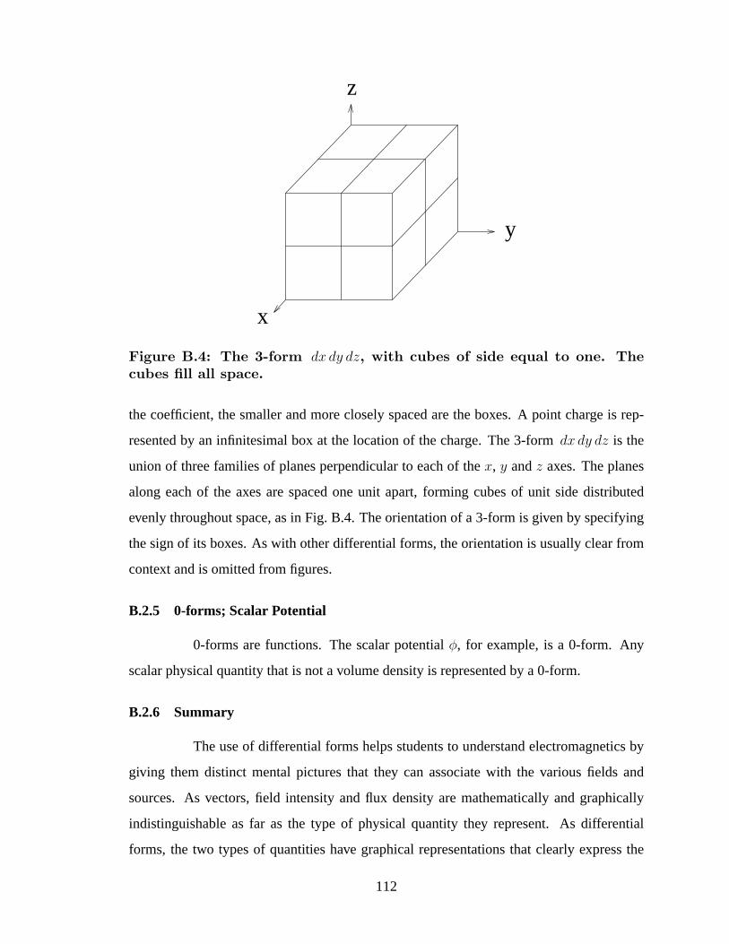
y
z
x
Figure B.4: The 3-form dx dy dz, with cubes of side equal to one. Thecubes fill all space.
the coefficient, the smaller and more closely spaced are the boxes. A point charge is rep-
resented by an infinitesimal box at the location of the charge. The 3-formdx dy dz is the
union of three families of planes perpendicular to each of thex, y andz axes. The planes
along each of the axes are spaced one unit apart, forming cubes of unit side distributed
evenly throughout space, as in Fig. B.4. The orientation of a 3-form is given by specifying
the sign of its boxes. As with other differential forms, the orientation is usually clear from
context and is omitted from figures.
B.2.5 0-forms; Scalar Potential
0-forms are functions. The scalar potentialφ, for example, is a 0-form. Any
scalar physical quantity that is not a volume density is represented by a 0-form.
B.2.6 Summary
The use of differential forms helps students to understand electromagnetics by
giving them distinct mental pictures that they can associate with the various fields and
sources. As vectors, field intensity and flux density are mathematically and graphically
indistinguishable as far as the type of physical quantity they represent. As differential
forms, the two types of quantities have graphical representations that clearly express the
112
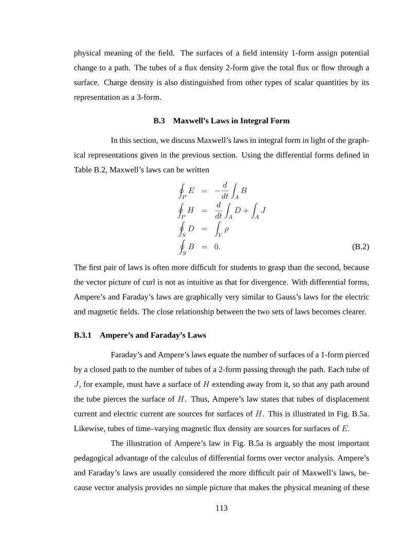
physical meaning of the field. The surfaces of a field intensity 1-form assign potential
change to a path. The tubes of a flux density 2-form give the total flux or flow through a
surface. Charge density is also distinguished from other types of scalar quantities by its
representation as a 3-form.
B.3 Maxwell’s Laws in Integral Form
In this section, we discuss Maxwell’s laws in integral form in light of the graph-
ical representations given in the previous section. Using the differential forms defined in
Table B.2, Maxwell’s laws can be written∮
PE = − d
dt
∫
AB
∮
PH =
d
dt
∫
AD +
∫
AJ
∮
SD =
∫
Vρ
∮
SB = 0. (B.2)
The first pair of laws is often more difficult for students to grasp than the second, because
the vector picture of curl is not as intuitive as that for divergence. With differential forms,
Ampere’s and Faraday’s laws are graphically very similar to Gauss’s laws for the electric
and magnetic fields. The close relationship between the two sets of laws becomes clearer.
B.3.1 Ampere’s and Faraday’s Laws
Faraday’s and Ampere’s laws equate the number of surfaces of a 1-form pierced
by a closed path to the number of tubes of a 2-form passing through the path. Each tube of
J , for example, must have a surface ofH extending away from it, so that any path around
the tube pierces the surface ofH. Thus, Ampere’s law states that tubes of displacement
current and electric current are sources for surfaces ofH. This is illustrated in Fig. B.5a.
Likewise, tubes of time–varying magnetic flux density are sources for surfaces ofE.
The illustration of Ampere’s law in Fig. B.5a is arguably the most important
pedagogical advantage of the calculus of differential forms over vector analysis. Ampere’s
and Faraday’s laws are usually considered the more difficult pair of Maxwell’s laws, be-
cause vector analysis provides no simple picture that makes the physical meaning of these
113

laws intuitive. Compare Fig. B.5a to the vector representation of the same field in Fig. B.5b.
The vector field appears to “curl” everywhere in space. Students must be convinced that
indeed the field has no curl except at the location of the current, using some pedagogical
device such as an imaginary paddle wheel in a rotating fluid. The surfaces ofH, on the
other hand, end only along the tubes of current; where they do not end, the field has no
curl. This is the fundamental concept underlying Ampere’s and Faraday’s laws: tubes of
time varying flux or current produce field intensity surfaces.
(a) (b)
Figure B.5: (a) A graphical representation of Ampere’s law: tubes ofcurrent produce surfaces of magnetic field intensity. Any loop aroundthe three tubes of J must pierce three surfaces of H. (b) A cross sectionof the same magnetic field using vectors. The vector field appears to“curl” everywhere, even though the field has nonzero curl only at thelocation of the current.
B.3.2 Gauss’s Laws
Gauss’s law for the electric field states that the number of tubes ofD flowing
out through a closed surface must be equal to the number of boxes ofρ inside the surface.
The boxes ofρ are sources for the tubes ofD, as shown in Fig. B.6. Gauss’s law for the
magnetic flux density states that tubes of the 2-formB can never end—they must either
form closed loops or go off to infinity.
Comparing Figs. B.5a and B.6 shows the close relationship between the two
sets of Maxwell’s laws. In the same way that flux density tubes are produced by boxes of
114
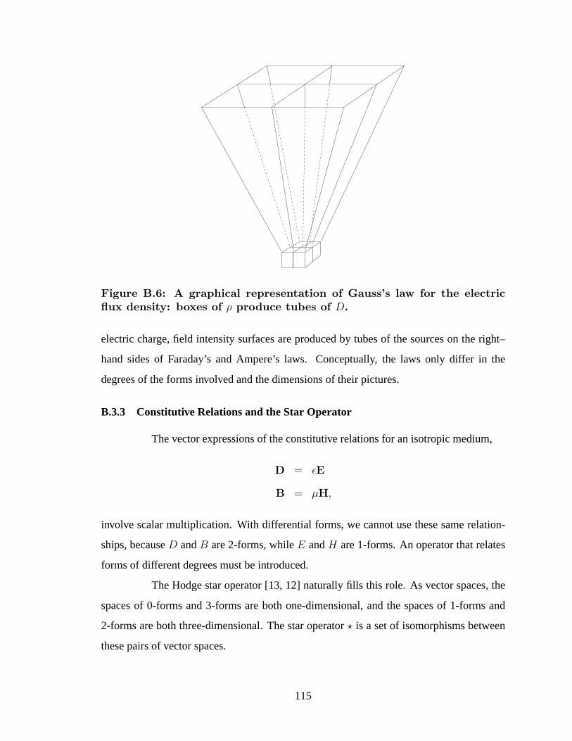
Figure B.6: A graphical representation of Gauss’s law for the electricflux density: boxes of ρ produce tubes of D.
electric charge, field intensity surfaces are produced by tubes of the sources on the right–
hand sides of Faraday’s and Ampere’s laws. Conceptually, the laws only differ in the
degrees of the forms involved and the dimensions of their pictures.
B.3.3 Constitutive Relations and the Star Operator
The vector expressions of the constitutive relations for an isotropic medium,
D = εE
B = µH,
involve scalar multiplication. With differential forms, we cannot use these same relation-
ships, becauseD andB are 2-forms, whileE andH are 1-forms. An operator that relates
forms of different degrees must be introduced.
The Hodge star operator [13, 12] naturally fills this role. As vector spaces, the
spaces of 0-forms and 3-forms are both one-dimensional, and the spaces of 1-forms and
2-forms are both three-dimensional. The star operator? is a set of isomorphisms between
these pairs of vector spaces.
115
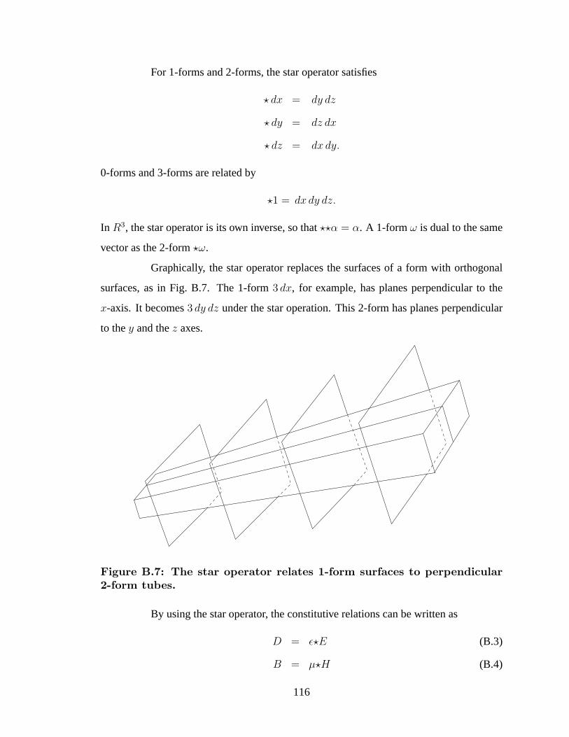
For 1-forms and 2-forms, the star operator satisfies
? dx = dy dz
? dy = dz dx
? dz = dx dy.
0-forms and 3-forms are related by
?1 = dx dy dz.
In R3, the star operator is its own inverse, so that??α = α. A 1-form ω is dual to the same
vector as the 2-form?ω.
Graphically, the star operator replaces the surfaces of a form with orthogonal
surfaces, as in Fig. B.7. The 1-form3 dx, for example, has planes perpendicular to the
x-axis. It becomes3 dy dz under the star operation. This 2-form has planes perpendicular
to they and thez axes.
Figure B.7: The star operator relates 1-form surfaces to perpendicular2-form tubes.
By using the star operator, the constitutive relations can be written as
D = ε?E (B.3)
B = µ?H (B.4)
116
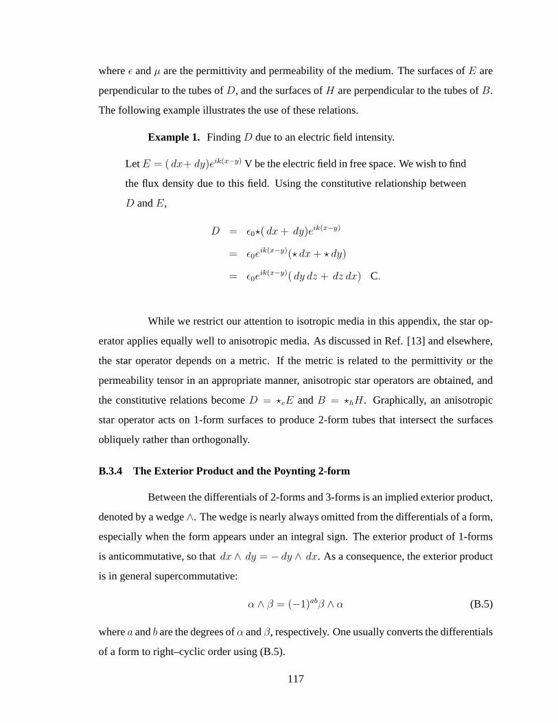
whereε andµ are the permittivity and permeability of the medium. The surfaces ofE are
perpendicular to the tubes ofD, and the surfaces ofH are perpendicular to the tubes ofB.
The following example illustrates the use of these relations.
Example 1. FindingD due to an electric field intensity.
LetE = ( dx+ dy)eik(x−y) V be the electric field in free space. We wish to find
the flux density due to this field. Using the constitutive relationship between
D andE,
D = ε0?( dx + dy)eik(x−y)
= ε0eik(x−y)(? dx + ? dy)
= ε0eik(x−y)( dy dz + dz dx) C.
While we restrict our attention to isotropic media in this appendix, the star op-
erator applies equally well to anisotropic media. As discussed in Ref. [13] and elsewhere,
the star operator depends on a metric. If the metric is related to the permittivity or the
permeability tensor in an appropriate manner, anisotropic star operators are obtained, and
the constitutive relations becomeD = ?eE andB = ?hH. Graphically, an anisotropic
star operator acts on 1-form surfaces to produce 2-form tubes that intersect the surfaces
obliquely rather than orthogonally.
B.3.4 The Exterior Product and the Poynting 2-form
Between the differentials of 2-forms and 3-forms is an implied exterior product,
denoted by a wedge∧. The wedge is nearly always omitted from the differentials of a form,
especially when the form appears under an integral sign. The exterior product of 1-forms
is anticommutative, so thatdx ∧ dy = − dy ∧ dx. As a consequence, the exterior product
is in general supercommutative:
α ∧ β = (−1)abβ ∧ α (B.5)
wherea andb are the degrees ofα andβ, respectively. One usually converts the differentials
of a form to right–cyclic order using (B.5).
117
As a consequence of (B.5), any differential form with a repeated differential
vanishes. In a three-dimensional space each term of ap-form will always contain a repeated
differential if p > 3, so there are no nonzerop-forms forp > 3.
The exterior product of two 1-forms is analogous to the vector cross product.
With vector analysis, it is not obvious that the cross product of vectors is a different type
of quantity than the factors. Under coordinate inversion,a × b changes sign relative to
a vector with the same components, so thata × b is a pseudovector. With forms, the
distinction betweena ∧ b anda or b individually is clear.
The exterior product of a 1-form and a 2-form corresponds to the dot product.
The coefficient of the resulting 3-form is equal to the dot product of the vector fields dual
to the 1-form and 2-form in the euclidean metric.
Combinations of cross and dot products are somewhat difficult to manipulate
algebraically, often requiring the use of tabulated identities. Using the supercommutativity
of the exterior product, the student can easily manipulate arbitrary products of forms. For
example, the identities
A · (B×C) = C · (A×B) = B · (C×A)
are in the euclidean metric equivalent to relationships which are easily obtained from (B.5).
Factors in any exterior product can be interchanged arbitrarily as long as the sign of the
product is changed according to (B.5).
Consider the exterior product of the 1-formsE andH,
E ∧H = (E1 dx + E2 dy + E3 dz) ∧ (H1 dx + H2 dy + H3 dz)
= E1H1 dx dx + E1H2 dx dy + E1H3 dx dz
+E2H1 dy dx + E2H2 dy dy + E2H3 dy dz
+E3H1 dz dx + E3H2 dz dy + E3H3 dz dz
= (E2H3 − E3H2) dy dz + (E3H1 − E1H3) dz dx + (E1H2 − E2H1) dx dy.
This is the Poynting 2-formS. For complex fields,S = E ∧H∗. For time–varying fields,
the tubes of this 2-form represent flow of electromagnetic power, as shown in Fig. B.8. The
sides of the tubes are the surfaces ofE andH. This gives a clear geometrical interpretation
118
to the fact that the direction of power flow is orthogonal to the orientations of bothE and
H.
Power
E
H
Figure B.8: The Poynting power flow 2-form S = E ∧H. Surfaces of the1-forms E and H are the sides of the tubes of S.
Example 2. The Poynting 2-form due to a plane wave.
Consider a plane wave propagating in free space in thez direction, with the
time–harmonic electric fieldE = E0dx V in the x direction. The Poynting
2-form is
S = E ∧H
= E0 dx ∧ E0
η0
dy
=E2
0
η0
dx dy W
whereη0 is the wave impedance of free space.
119
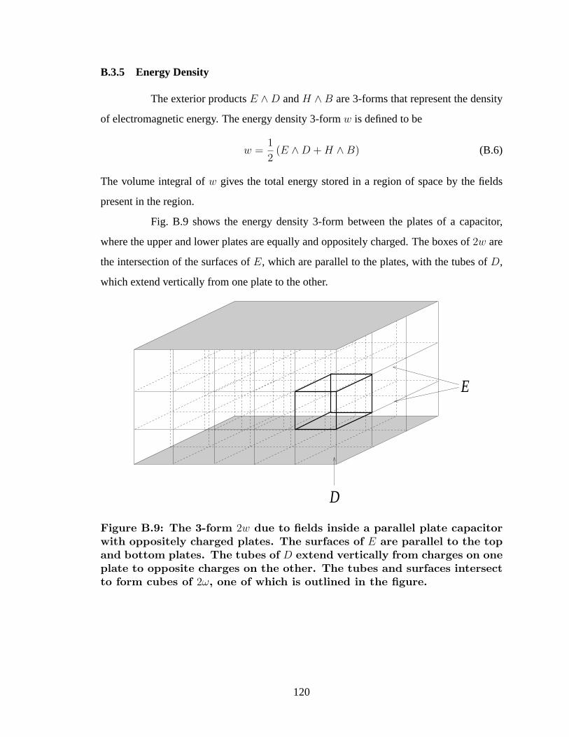
B.3.5 Energy Density
The exterior productsE ∧D andH ∧ B are 3-forms that represent the density
of electromagnetic energy. The energy density 3-formw is defined to be
w =1
2(E ∧D + H ∧B) (B.6)
The volume integral ofw gives the total energy stored in a region of space by the fields
present in the region.
Fig. B.9 shows the energy density 3-form between the plates of a capacitor,
where the upper and lower plates are equally and oppositely charged. The boxes of2w are
the intersection of the surfaces ofE, which are parallel to the plates, with the tubes ofD,
which extend vertically from one plate to the other.
D
E
Figure B.9: The 3-form 2w due to fields inside a parallel plate capacitorwith oppositely charged plates. The surfaces of E are parallel to the topand bottom plates. The tubes of D extend vertically from charges on oneplate to opposite charges on the other. The tubes and surfaces intersectto form cubes of 2ω, one of which is outlined in the figure.
120
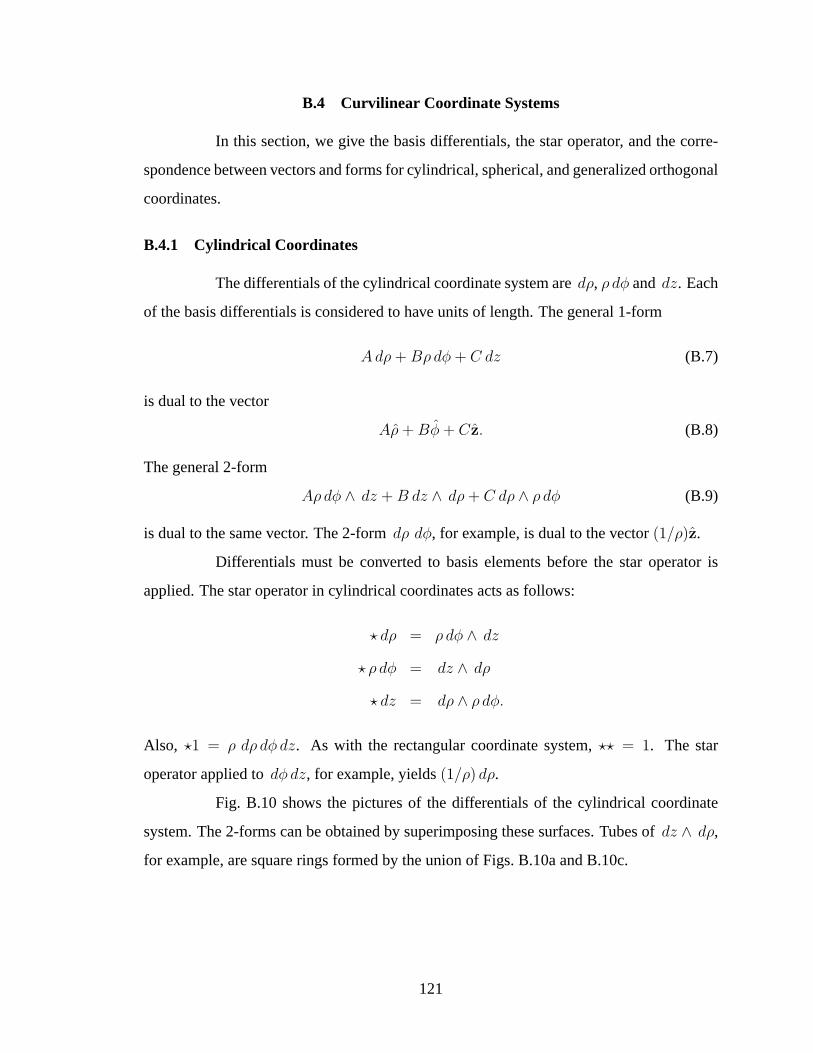
B.4 Curvilinear Coordinate Systems
In this section, we give the basis differentials, the star operator, and the corre-
spondence between vectors and forms for cylindrical, spherical, and generalized orthogonal
coordinates.
B.4.1 Cylindrical Coordinates
The differentials of the cylindrical coordinate system aredρ, ρ dφ and dz. Each
of the basis differentials is considered to have units of length. The general 1-form
A dρ + Bρ dφ + C dz (B.7)
is dual to the vector
Aρ + Bφ + Cz. (B.8)
The general 2-form
Aρdφ ∧ dz + B dz ∧ dρ + C dρ ∧ ρ dφ (B.9)
is dual to the same vector. The 2-formdρ dφ, for example, is dual to the vector(1/ρ)z.
Differentials must be converted to basis elements before the star operator is
applied. The star operator in cylindrical coordinates acts as follows:
? dρ = ρ dφ ∧ dz
? ρ dφ = dz ∧ dρ
? dz = dρ ∧ ρ dφ.
Also, ?1 = ρ dρ dφ dz. As with the rectangular coordinate system,?? = 1. The star
operator applied todφ dz, for example, yields(1/ρ) dρ.
Fig. B.10 shows the pictures of the differentials of the cylindrical coordinate
system. The 2-forms can be obtained by superimposing these surfaces. Tubes ofdz ∧ dρ,
for example, are square rings formed by the union of Figs. B.10a and B.10c.
121
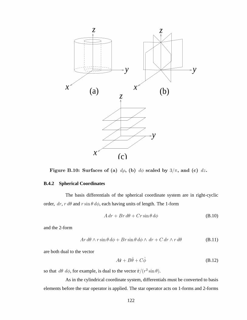
(a)
z
y
x
(c)
(b)
z
y
x
x
y
z
Figure B.10: Surfaces of (a) dρ, (b) dφ scaled by 3/π, and (c) dz.
B.4.2 Spherical Coordinates
The basis differentials of the spherical coordinate system are in right-cyclic
order, dr, r dθ andr sin θ dφ, each having units of length. The 1-form
Adr + Br dθ + Cr sin θ dφ (B.10)
and the 2-form
Ar dθ ∧ r sin θ dφ + Br sin θ dφ ∧ dr + C dr ∧ r dθ (B.11)
are both dual to the vector
Ar + Bθ + Cφ (B.12)
so thatdθ dφ, for example, is dual to the vectorr/(r2 sin θ).
As in the cylindrical coordinate system, differentials must be converted to basis
elements before the star operator is applied. The star operator acts on 1-forms and 2-forms
122
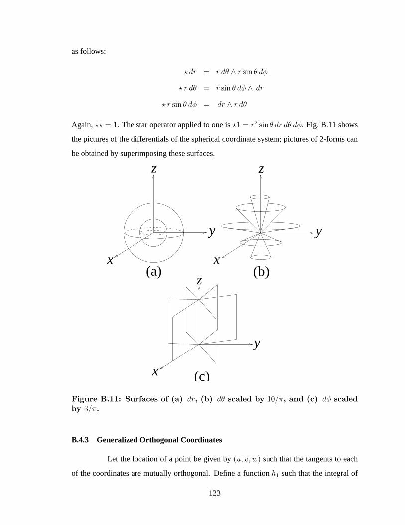
as follows:
? dr = r dθ ∧ r sin θ dφ
? r dθ = r sin θ dφ ∧ dr
? r sin θ dφ = dr ∧ r dθ
Again,?? = 1. The star operator applied to one is?1 = r2 sin θ dr dθ dφ. Fig. B.11 shows
the pictures of the differentials of the spherical coordinate system; pictures of 2-forms can
be obtained by superimposing these surfaces.
y
z
x(a) (b)
z
y
x (c)
y
x
z
Figure B.11: Surfaces of (a) dr, (b) dθ scaled by 10/π, and (c) dφ scaledby 3/π.
B.4.3 Generalized Orthogonal Coordinates
Let the location of a point be given by(u, v, w) such that the tangents to each
of the coordinates are mutually orthogonal. Define a functionh1 such that the integral of
123
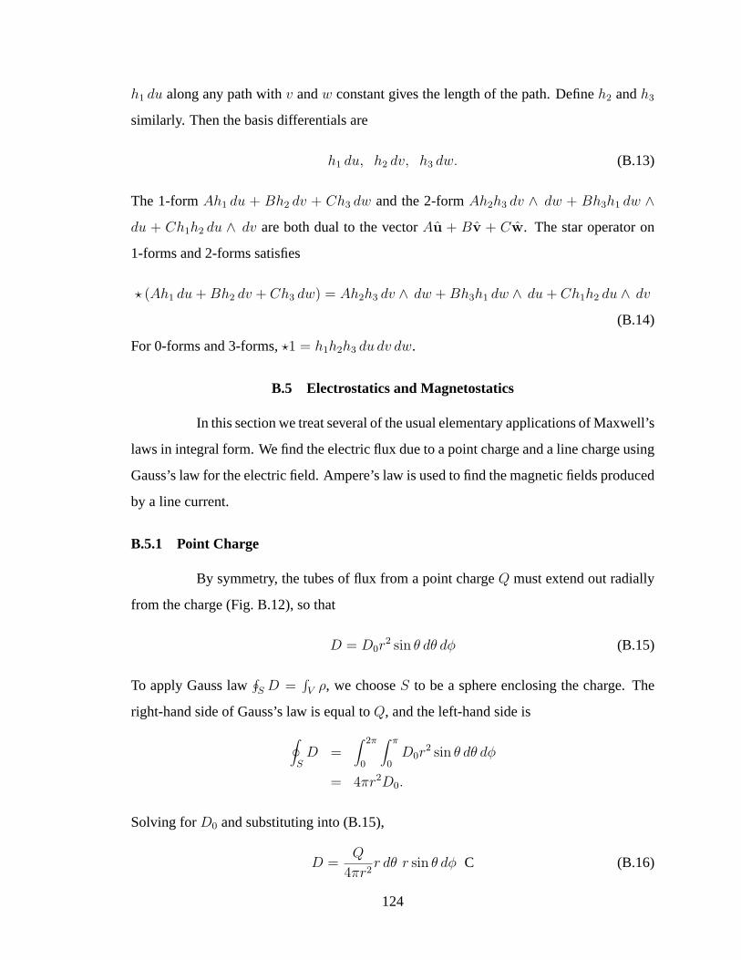
h1 du along any path withv andw constant gives the length of the path. Defineh2 andh3
similarly. Then the basis differentials are
h1 du, h2 dv, h3 dw. (B.13)
The 1-formAh1 du + Bh2 dv + Ch3 dw and the 2-formAh2h3 dv ∧ dw + Bh3h1 dw ∧du + Ch1h2 du ∧ dv are both dual to the vectorAu + Bv + Cw. The star operator on
1-forms and 2-forms satisfies
? (Ah1 du + Bh2 dv + Ch3 dw) = Ah2h3 dv ∧ dw + Bh3h1 dw ∧ du + Ch1h2 du ∧ dv
(B.14)
For 0-forms and 3-forms,?1 = h1h2h3 du dv dw.
B.5 Electrostatics and Magnetostatics
In this section we treat several of the usual elementary applications of Maxwell’s
laws in integral form. We find the electric flux due to a point charge and a line charge using
Gauss’s law for the electric field. Ampere’s law is used to find the magnetic fields produced
by a line current.
B.5.1 Point Charge
By symmetry, the tubes of flux from a point chargeQ must extend out radially
from the charge (Fig. B.12), so that
D = D0r2 sin θ dθ dφ (B.15)
To apply Gauss law∮S D =
∫V ρ, we chooseS to be a sphere enclosing the charge. The
right-hand side of Gauss’s law is equal toQ, and the left-hand side is
∮
SD =
∫ 2π
0
∫ π
0D0r
2 sin θ dθ dφ
= 4πr2D0.
Solving forD0 and substituting into (B.15),
D =Q
4πr2r dθ r sin θ dφ C (B.16)
124
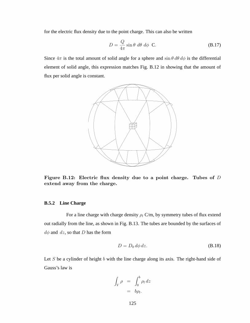
for the electric flux density due to the point charge. This can also be written
D =Q
4πsin θ dθ dφ C. (B.17)
Since4π is the total amount of solid angle for a sphere andsin θ dθ dφ is the differential
element of solid angle, this expression matches Fig. B.12 in showing that the amount of
flux per solid angle is constant.
Figure B.12: Electric flux density due to a point charge. Tubes of Dextend away from the charge.
B.5.2 Line Charge
For a line charge with charge densityρl C/m, by symmetry tubes of flux extend
out radially from the line, as shown in Fig. B.13. The tubes are bounded by the surfaces of
dφ and dz, so thatD has the form
D = D0 dφ dz. (B.18)
Let S be a cylinder of heightb with the line charge along its axis. The right-hand side of
Gauss’s law is
∫
Vρ =
∫ b
0ρl dz
= bρl.
125
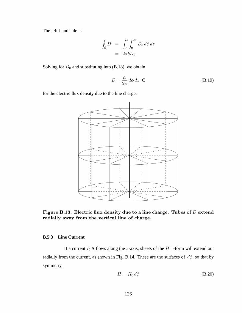
The left-hand side is
∮
SD =
∫ b
0
∫ 2π
0D0 dφ dz
= 2πbD0.
Solving forD0 and substituting into (B.18), we obtain
D =ρl
2πdφ dz C (B.19)
for the electric flux density due to the line charge.
Figure B.13: Electric flux density due to a line charge. Tubes of D extendradially away from the vertical line of charge.
B.5.3 Line Current
If a currentIl A flows along thez-axis, sheets of theH 1-form will extend out
radially from the current, as shown in Fig. B.14. These are the surfaces ofdφ, so that by
symmetry,
H = H0 dφ (B.20)
126

whereH0 is a constant we need to find using Ampere’s law. We choose the pathP in
Ampere’s law∮P H = d
dt
∫A D +
∫A J to be a loop around thez-axis. Assuming that
D = 0, the right–hand side of Ampere’s law is equal toIl. The left-hand side is the integral
of H over the loop,
∮
PH =
∫ 2π
0H0 dφ
= 2πH0.
The magnetic field intensity is then
H =Il
2πdφ A (B.21)
for the line current source.
Figure B.14: Magnetic field intensity H due to a line current.
B.6 The Exterior Derivative and Maxwell’s Laws in Point Form
In this section we introduce the exterior derivative and the generalized Stokes
theorem and use these to express Maxwell’s laws in point form. The exterior derivative is
a single operator which has the gradient, curl, and divergence as special cases, depending
127
on the degree of the differential form on which the exterior derivative acts. The exterior
derivative has the symbold, and can be written formally as
d ≡ ∂
∂xdx +
∂
∂ydy +
∂
∂zdz. (B.22)
The exterior derivative can be thought of as implicit differentiation with new differentials
introduced from the left.
B.6.1 Exterior Derivative of 0-forms
Consider the 0-formf(x, y, z). If we implicitly differentiatef with respect to
each of the coordinates, we obtain
df =∂f
∂xdx +
∂f
∂ydy +
∂f
∂zdz. (B.23)
which is a 1-form, the exterior derivative off . Note that the differentialsdx, dy, and dz
are the exterior derivatives of the coordinate functionsx, y, andz. The 1-formdf is dual
to the gradient off .
If φ represents a scalar electric potential, the negative of its exterior derivative
is electric field intensity:
E = −dφ.
As noted earlier, the surfaces of the 1-formE are equipotentials, or level sets of the function
φ, so that the exterior derivative of a 0-form has a simple graphical interpretation.
B.6.2 Exterior Derivative of 1-forms
The exterior derivative of a 1-form is analogous to the vector curl operation. If
E is an arbitrary 1-formE1 dx + E2 dy + E3 dz, then the exterior derivative ofE is
dE =(
∂∂x
E1 dx + ∂∂y
E1 dy + ∂∂z
E1 dz)
dx
+(
∂∂x
E2 dx + ∂∂y
E2 dy + ∂∂z
E2 dz)
dy
+(
∂∂x
E3 dx + ∂∂y
E3 dy + ∂∂z
E3 dz)
dz
Using the antisymmetry of the exterior product, this becomes
dE = (∂E3
∂y− ∂E2
∂z) dy dz + (
∂E1
∂z− ∂E3
∂x) dz dx + (
∂E2
∂x− ∂E1
∂y) dx dy, (B.24)
128
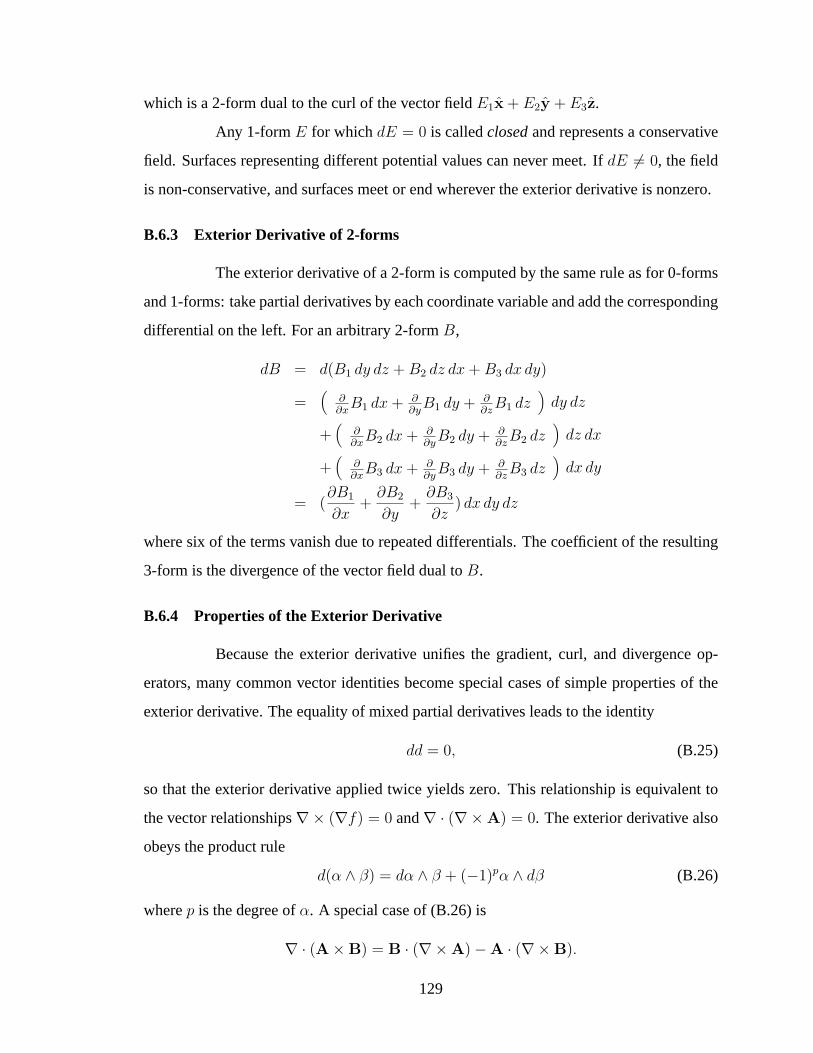
which is a 2-form dual to the curl of the vector fieldE1x + E2y + E3z.
Any 1-formE for whichdE = 0 is calledclosedand represents a conservative
field. Surfaces representing different potential values can never meet. IfdE 6= 0, the field
is non-conservative, and surfaces meet or end wherever the exterior derivative is nonzero.
B.6.3 Exterior Derivative of 2-forms
The exterior derivative of a 2-form is computed by the same rule as for 0-forms
and 1-forms: take partial derivatives by each coordinate variable and add the corresponding
differential on the left. For an arbitrary 2-formB,
dB = d(B1 dy dz + B2 dz dx + B3 dx dy)
=(
∂∂x
B1 dx + ∂∂y
B1 dy + ∂∂z
B1 dz)
dy dz
+(
∂∂x
B2 dx + ∂∂y
B2 dy + ∂∂z
B2 dz)
dz dx
+(
∂∂x
B3 dx + ∂∂y
B3 dy + ∂∂z
B3 dz)
dx dy
= (∂B1
∂x+
∂B2
∂y+
∂B3
∂z) dx dy dz
where six of the terms vanish due to repeated differentials. The coefficient of the resulting
3-form is the divergence of the vector field dual toB.
B.6.4 Properties of the Exterior Derivative
Because the exterior derivative unifies the gradient, curl, and divergence op-
erators, many common vector identities become special cases of simple properties of the
exterior derivative. The equality of mixed partial derivatives leads to the identity
dd = 0, (B.25)
so that the exterior derivative applied twice yields zero. This relationship is equivalent to
the vector relationships∇× (∇f) = 0 and∇ · (∇×A) = 0. The exterior derivative also
obeys the product rule
d(α ∧ β) = dα ∧ β + (−1)pα ∧ dβ (B.26)
wherep is the degree ofα. A special case of (B.26) is
∇ · (A×B) = B · (∇×A)−A · (∇×B).
129
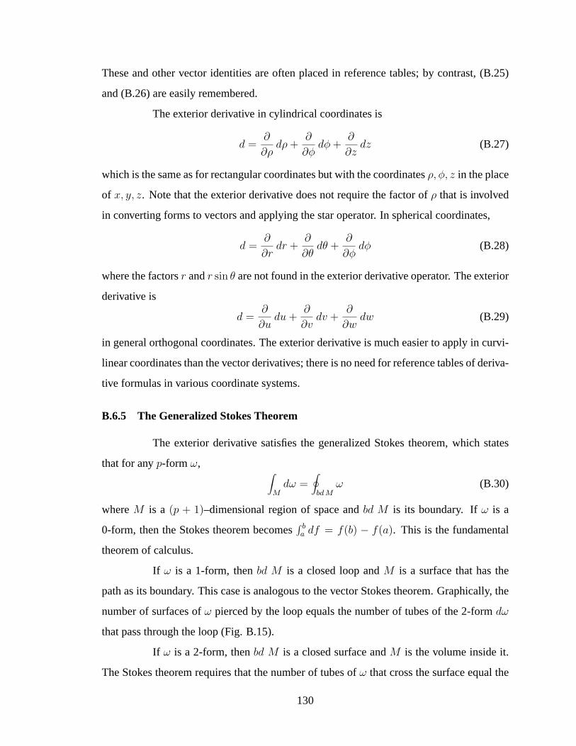
These and other vector identities are often placed in reference tables; by contrast, (B.25)
and (B.26) are easily remembered.
The exterior derivative in cylindrical coordinates is
d =∂
∂ρdρ +
∂
∂φdφ +
∂
∂zdz (B.27)
which is the same as for rectangular coordinates but with the coordinatesρ, φ, z in the place
of x, y, z. Note that the exterior derivative does not require the factor ofρ that is involved
in converting forms to vectors and applying the star operator. In spherical coordinates,
d =∂
∂rdr +
∂
∂θdθ +
∂
∂φdφ (B.28)
where the factorsr andr sin θ are not found in the exterior derivative operator. The exterior
derivative is
d =∂
∂udu +
∂
∂vdv +
∂
∂wdw (B.29)
in general orthogonal coordinates. The exterior derivative is much easier to apply in curvi-
linear coordinates than the vector derivatives; there is no need for reference tables of deriva-
tive formulas in various coordinate systems.
B.6.5 The Generalized Stokes Theorem
The exterior derivative satisfies the generalized Stokes theorem, which states
that for anyp-form ω, ∫
Mdω =
∮
bd Mω (B.30)
whereM is a (p + 1)–dimensional region of space andbd M is its boundary. Ifω is a
0-form, then the Stokes theorem becomes∫ ba df = f(b) − f(a). This is the fundamental
theorem of calculus.
If ω is a 1-form, thenbd M is a closed loop andM is a surface that has the
path as its boundary. This case is analogous to the vector Stokes theorem. Graphically, the
number of surfaces ofω pierced by the loop equals the number of tubes of the 2-formdω
that pass through the loop (Fig. B.15).
If ω is a 2-form, thenbd M is a closed surface andM is the volume inside it.
The Stokes theorem requires that the number of tubes ofω that cross the surface equal the
130
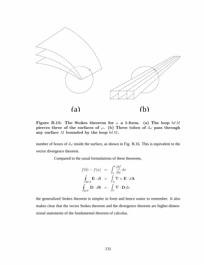
(b)(a)
Figure B.15: The Stokes theorem for ω a 1-form. (a) The loop bdMpierces three of the surfaces of ω. (b) Three tubes of dω pass throughany surface M bounded by the loop bdM .
number of boxes ofdω inside the surface, as shown in Fig. B.16. This is equivalent to the
vector divergence theorem.
Compared to the usual formulations of these theorems,
f(b)− f(a) =∫ b
a
∂f
∂xdx
∮
bd AE · dl =
∫
A∇× E · dA
∮
bd VD · dS =
∫
V∇ ·D dv
the generalized Stokes theorem is simpler in form and hence easier to remember. It also
makes clear that the vector Stokes theorem and the divergence theorem are higher-dimen-
sional statements of the fundamental theorem of calculus.
131
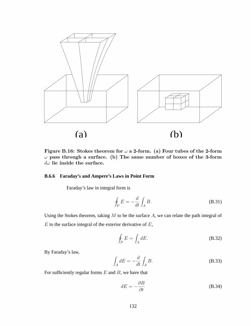
(b)(a)
Figure B.16: Stokes theorem for ω a 2-form. (a) Four tubes of the 2-formω pass through a surface. (b) The same number of boxes of the 3-formdω lie inside the surface.
B.6.6 Faraday’s and Ampere’s Laws in Point Form
Faraday’s law in integral form is
∮
PE = − d
dt
∫
AB. (B.31)
Using the Stokes theorem, takingM to be the surfaceA, we can relate the path integral of
E to the surface integral of the exterior derivative ofE,
∮
PE =
∫
AdE. (B.32)
By Faraday’s law, ∫
AdE = − d
dt
∫
AB. (B.33)
For sufficiently regular formsE andB, we have that
dE = −∂B
∂t(B.34)
132

since (B.33) is valid for all surfacesA. This is Faraday’s law in point form. This law states
that new surfaces ofE are produced by tubes of time–varying magnetic flux.
Using the same argument, Ampere’s law becomes
dH =∂D
∂t+ J. (B.35)
Ampere’s law shows that new surfaces ofH are produced by tubes of time–varying electric
flux or electric current.
B.6.7 Gauss’s Laws in Point Form
Gauss’s law for the electric flux density is∮
SD =
∫
Vρ. (B.36)
The Stokes theorem withM as the volumeV andbd M as the surfaceS shows that∮
SD =
∫
VdD. (B.37)
Using Gauss’s law in integral form (B.36),∫
VdD =
∫
Vρ. (B.38)
We can then write
dD = ρ. (B.39)
This is Gauss’s law for the electric field in point form. Graphically, this law shows that
tubes of electric flux density can end only on electric charges. Similarly, Gauss’s law for
the magnetic field is
dB = 0. (B.40)
This law requires that tubes of magnetic flux density never end; they must form closed
loops or extend to infinity.
B.6.8 Poynting’s Theorem
Using Maxwell’s laws, we can derive a conservation law for electromagnetic
energy. The exterior derivative ofS is
dS = d(E ∧H)
= (dE) ∧H − E ∧ (dH)
133

Using Ampere’s and Faraday’s laws, this can be written
dS = −∂B
∂t∧H − E ∧ ∂D
∂t− E ∧ J (B.41)
Finally, using the definition (B.6) ofw, this becomes
dS = −∂w
∂t− E ∧ J. (B.42)
At a point where no sources exist, a change in stored electromagnetic energy must be
accompanied by tubes ofS that represent flow of energy towards or away from the point.
B.6.9 Integrating Forms by Pullback
We have seen in previous sections that differential forms give integration a clear
graphical interpretation. The use of differential forms also results in several simplifications
of the integration process itself. Integrals of vector fields require a metric; integrals of
differential forms do not. The method of pullback replaces the computation of differential
length and surface elements that is required before a vector field can be integrated.
Consider the path integral
∫
PE · dl. (B.43)
The dot product ofE with dl produces a 1-form with a single differential in the parameter
of the pathP , allowing the integral to be evaluated. The integral of the 1-formE dual to
E over the same path is computed by the method ofpullback, as change of variables for
differential forms is commonly termed. Let the pathP be parameterized by
x = p1(t), y = p2(t), z = p3(t)
for a < t < b. The pullback ofE to the pathP is denotedP ∗E, and is defined to be
P ∗E = P ∗(E1 dx + E2 dy + E3 dz)
= E1(p1, p2, p3)dp1 + E2(p1, p2, p3)dp2 + E3(p1, p2, p3)dp3.
=
(E1(p1, p2, p3)
∂p1
∂t+ E2(p1, p2, p3)
∂p2
∂t+ E3(p1, p2, p3)
∂p3
∂t
)dt.
134

Using the pullback ofE, we convert the integral overP to an integral int over the interval
[a, b], ∫
PE =
∫ b
aP ∗E (B.44)
Components of the Jacobian matrix of the coordinate transform from the original coordi-
nate system to the parameterization of the region of integration enter naturally when the
exterior derivatives are performed. Pullback works similarly for 2-forms and 3-forms, al-
lowing evaluation of surface and volume integrals by the same method. The following
example illustrates the use of pullback.
Example 3. Work required to move a charge through an electric field.
Let the electric field intensity be given byE = 2xy dx + x2 dy− dz. A charge
of q = 1 C is transported over the pathP given by(x = t2, y = t, z = 1− t3)
from t = 0 to t = 1. The work required is given by
W = −q∫
P2xy dx + x2 dy − dz (B.45)
which by Eq. (B.44) is equal to
= −q∫ 1
0P ∗(2xy dx + x2 dy − dz)
whereP ∗E is the pullback of the field 1-form to the pathP ,
P ∗E = 2(t2)(t)2t dt + (t2)2 dt− (−3t2) dt
= (5t4 + 3t2) dt.
Integrating this new 1-form int over [0, 1], we obtain
W = −∫ 1
0(5t4 + 3t2)dt = −2 J
as the total work required to move the charge alongP .
135
B.6.10 Existence of Graphical Representations
With the exterior derivative, a condition can be given for the existence of the
graphical representations of Sec. B.2. These representations do not correspond to the usual
“tangent space” picture of a vector field, but rather are analogous to the integral curves
of a vector field. Obtaining the graphical representation of a differential form as a family
of surfaces is in general nontrivial, and is closely related to Pfaff’s problem [51]. By the
solution to Pfaff’s problem, each differential form may be represented graphically in two
dimensions as families of lines. In three dimensions, a 1-formω can be represented as
surfaces if the rotationω∧ dω is zero. Ifω∧ dω 6= 0, then there exist local coordinates for
whichω has the formdu + v dw, so that it is the sum of two 1-forms, both of which can be
graphically represented as surfaces.
An arbitrary, smooth 2-form in R3 can be written locally in the formfdg ∧ dh,
so that the 2-form consists of tubes ofdg ∧ dh scaled byf .
B.6.11 Summary
Throughout this section, we have noted various aspects of the calculus of dif-
ferential forms that simplify manipulations and provide insight into the principles of elec-
tromagnetics. The exterior derivative behaves differently depending on the degree of the
form it operates on, so that physical properties of a field are encoded in the type of form
used to represent it, rather than in the type of operator used to take its derivative. The
generalized Stokes theorem gives the vector Stokes theorem and the divergence theorem
intuitive graphical interpretations that illuminate the relationship between the two theo-
rems. While of lesser pedagogical importance, the algebraic and computational advantages
of forms cited in this section also aid students by reducing the need for reference tables or
memorization of identities.
136
B.7 The Interior Product and Boundary Conditions
Boundary conditions can be expressed using a combination of the exterior and
interior products. The same operator is used to express boundary conditions for field inten-
sities and flux densities, and in both cases the boundary conditions have simple graphical
interpretations.
B.7.1 The Interior Product
The interior product has the symbol. Graphically, the interior product re-
moves the surfaces of the first form from those of the second. The interior productdx dy
is zero, since there are nodx surfaces to remove. The interior product ofdx with itself is
one. The interior product ofdx and dx dy is dx dx dy = dy. To compute the interior
productdy dx dy, the differentialdy must be moved to the left ofdx dy before it can be
removed, so that
dy dx dy = − dy dy dx
= − dx.
The interior product of arbitrary 1-forms can be found by linearity from the relationships
dx dx = 1, dx dy = 0, dx dz = 0
dy dx = 0, dy dy = 1, dy dz = 0 (B.46)
dz dx = 0, dz dy = 0, dz dz = 1.
The interior product of a 1-form and a 2-form can be found using
dx dy ∧ dz = 0, dx dz ∧ dx = − dz, dx dx ∧ dy = dy
dy dy ∧ dz = dz, dy dz ∧ dx = 0, dy dx ∧ dy = − dx (B.47)
dz dy ∧ dz = − dy, dz dz ∧ dx = dx, dz dx ∧ dy = 0.
The following examples illustrate the use of the interior product.
Example 4. The Interior Product of two 1-forms
137
The interior product ofa = 3x dx− y dz andb = 4 dy + 5 dz is
a b = (3x dx− y dz) (4 dy + 5 dz)
= 12x dx dy + 15x dx dz − 4y dz dy − 5y dz dz
= −5y
which is the dot producta · b of the vectors dual to the 1-formsa andb.
Example 5. The Interior Product of a 1-form and a 2-form
The interior product ofa = 3x dx− y dz andc = 4 dz dx + 5 dx dy is
a c = (3x dx− y dz) (4 dz dx + 5 dx dy)
= 12x dx dz dx + 15x dx dx dy − 4y dz dz dx− 5y dz dx dy
= −12x dz + 15x dy − 4y dx
which is the 1-form dual to−a× c, wherea andc are dual toa andc.
The interior product can be related to the exterior product using the star operator.
The interior product of arbitrary formsa andb is
a b = ?(?b ∧ a) (B.48)
which can be used to compute the interior product in curvilinear coordinate systems. (This
formula shows the metric dependence of the interior product as we have defined it; the
interior product is usually defined to be the contraction of a vector with a form, which is
independent of any metric.) The interior and exterior products satisfy the identity
α = n ∧ (n α) + n (n ∧ α) (B.49)
wheren is a 1-form andα is arbitrary.
The Lorentz force law can be expressed using the interior product. The force
1-formF is
F = q(E − v B) (B.50)
138
wherev is the velocity of a chargeq, and the interior product can be computed by finding
the 1-form dual tov and using the rules given above.F is dual to the usual force vectorF.
The force 1-form has units of energy, and does not have as clear a physical interpretation
as the usual force vector. In this case we prefer to work with the vector dual toF , rather
thanF itself. Force, like displacement and velocity, is naturally a vector quantity.
B.7.2 Boundary Conditions
A boundary can be specified as the set of points satisfyingf(x, y, z) = 0 for
some suitable functionf . The surface normal 1-form is defined to be the normalized exte-
rior derivative off ,
n =df√
(df df). (B.51)
The surfaces ofn are parallel to the boundary. Using a subscript 1 to denote the region
wheref > 0, and a subscript 2 forf < 0, the four electromagnetic boundary conditions
can be written [2]
n (n ∧ (E1 − E2)) = 0
n (n ∧ (H1 −H2)) = Js
n (n ∧ (D1 −D2)) = ρs
n (n ∧ (B1 −B2)) = 0
whereJs is the surface current density 1-form andρs is the surface charge density 2-form.
The formn (n∧ω) is the component ofω which has surfaces perpendicular to the bound-
ary and integrates to the same value asω over any region lying in the boundary.
B.7.3 Surface Current
The action of the operatorn n∧ can be interpreted graphically, leading to a
simple picture of the field intensity boundary conditions. Consider the field discontinuity
H1 − H2 shown in Fig. B.17a. The exterior product ofn andH1 − H2 is a 2-form with
tubes that run parallel to the boundary, as shown in Fig. B.17b. The component ofH1−H2
with surfaces parallel to the boundary is removed. The interior productn (n∧ (H1−H2))
139
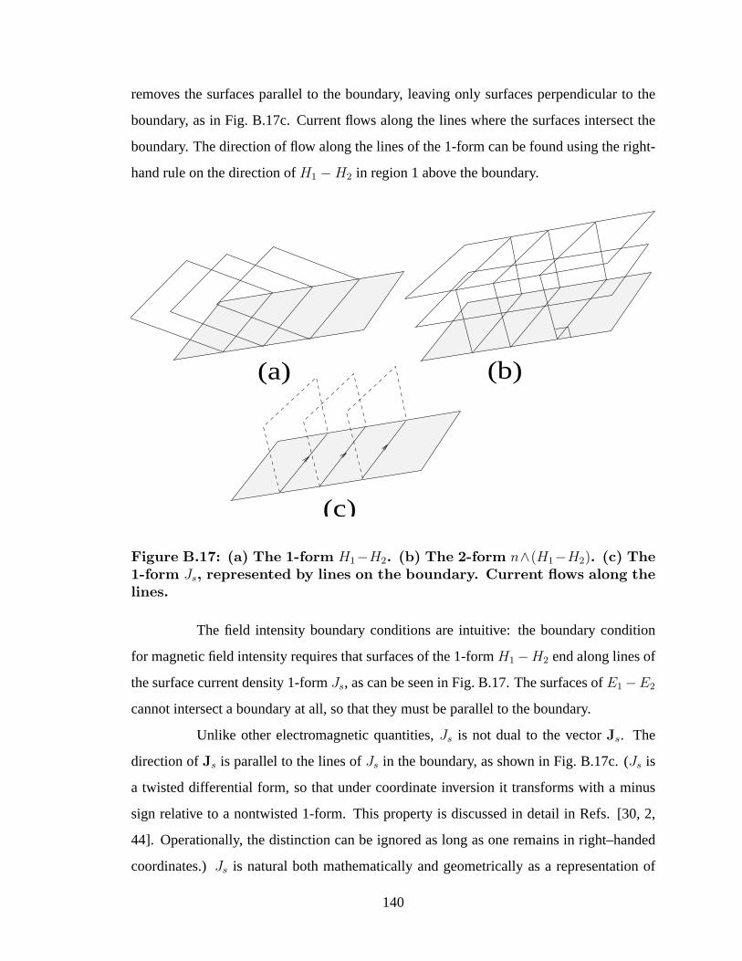
removes the surfaces parallel to the boundary, leaving only surfaces perpendicular to the
boundary, as in Fig. B.17c. Current flows along the lines where the surfaces intersect the
boundary. The direction of flow along the lines of the 1-form can be found using the right-
hand rule on the direction ofH1 −H2 in region 1 above the boundary.
(c)
(a) (b)
Figure B.17: (a) The 1-form H1−H2. (b) The 2-form n∧(H1−H2). (c) The1-form Js, represented by lines on the boundary. Current flows along thelines.
The field intensity boundary conditions are intuitive: the boundary condition
for magnetic field intensity requires that surfaces of the 1-formH1−H2 end along lines of
the surface current density 1-formJs, as can be seen in Fig. B.17. The surfaces ofE1−E2
cannot intersect a boundary at all, so that they must be parallel to the boundary.
Unlike other electromagnetic quantities,Js is not dual to the vectorJs. The
direction ofJs is parallel to the lines ofJs in the boundary, as shown in Fig. B.17c. (Js is
a twisted differential form, so that under coordinate inversion it transforms with a minus
sign relative to a nontwisted 1-form. This property is discussed in detail in Refs. [30, 2,
44]. Operationally, the distinction can be ignored as long as one remains in right–handed
coordinates.)Js is natural both mathematically and geometrically as a representation of
140
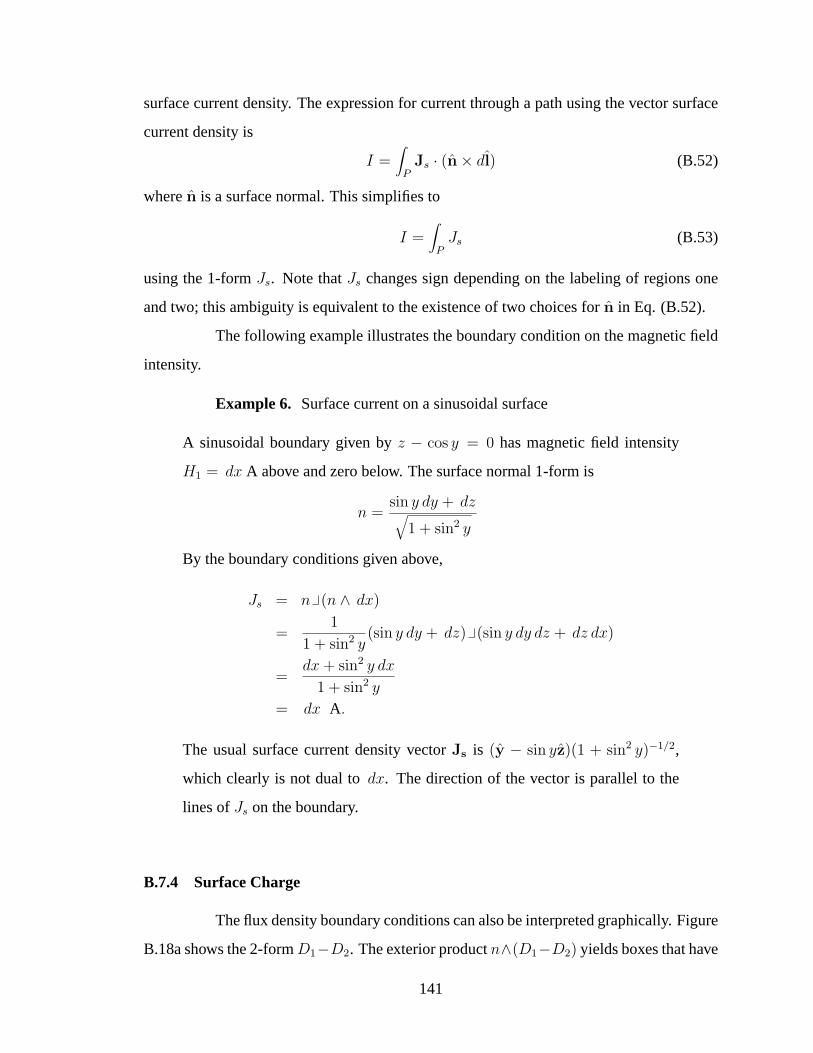
surface current density. The expression for current through a path using the vector surface
current density is
I =∫
PJs · (n× dl) (B.52)
wheren is a surface normal. This simplifies to
I =∫
PJs (B.53)
using the 1-formJs. Note thatJs changes sign depending on the labeling of regions one
and two; this ambiguity is equivalent to the existence of two choices forn in Eq. (B.52).
The following example illustrates the boundary condition on the magnetic field
intensity.
Example 6. Surface current on a sinusoidal surface
A sinusoidal boundary given byz − cos y = 0 has magnetic field intensity
H1 = dx A above and zero below. The surface normal 1-form is
n =sin y dy + dz√
1 + sin2 y
By the boundary conditions given above,
Js = n (n ∧ dx)
=1
1 + sin2 y(sin y dy + dz) (sin y dy dz + dz dx)
=dx + sin2 y dx
1 + sin2 y
= dx A.
The usual surface current density vectorJs is (y − sin yz)(1 + sin2 y)−1/2,
which clearly is not dual todx. The direction of the vector is parallel to the
lines ofJs on the boundary.
B.7.4 Surface Charge
The flux density boundary conditions can also be interpreted graphically. Figure
B.18a shows the 2-formD1−D2. The exterior productn∧(D1−D2) yields boxes that have
141
sides parallel to the boundary, as shown in Fig. B.18b. The component ofD1 − D2 with
tubes parallel to the boundary is removed by the exterior product. The interior product
with n removes the surfaces parallel to the boundary, leaving tubes perpendicular to the
boundary. These tubes intersect the boundary to form boxes of charge (Fig. B.18c). This is
the 2-formρs = n (n ∧ (D1 −D2)).
(c)
(a) (b)
Figure B.18: (a) The 2-form D1 −D2. (b) The 3-form n ∧ (D1 −D2), withsides perpendicular to the boundary. (c) The 2-form ρs, represented byboxes on the boundary.
The flux density boundary conditions have as clear a graphical interpretation as
those for field intensity: tubes of the differenceD1 −D2 in electric flux densities on either
side of a boundary intersect the boundary to form boxes of surface charge density. Tubes
of the discontinuity in magnetic flux density cannot intersect the boundary.
The sign of the charge on the boundary can be obtained from the direction of
D1 −D2 in region 1 above the boundary, which must point away from positive charge and
towards negative charge. The integral ofρs over a surface,
Q =∫
Sρs (B.54)
142

yields the total charge on the surface. Note thatρs changes sign depending on the labeling
of regions one and two. This ambiguity is equivalent to the existence of two choices for
the area elementdA and orientation of the areaA in the integral∫A qs dA, whereqs is the
usual scalar surface charge density. Often, the sign of the value of the integral is known
beforehand, and the subtlety goes unnoticed.
B.8 Conclusion
The primary pedagogical advantages of differential forms are the distinct repre-
sentations of field intensity and flux density, intuitive graphical representations of each of
Maxwell’s laws, and a simple picture of electromagnetic boundary conditions. Differential
forms provide visual models that can help students remember and apply the principles of
electromagnetics. Computational simplifications also result from the use of forms: deriva-
tives are easier to employ in curvilinear coordinates, integration becomes more straight-
forward, and families of related vector identities are replaced by algebraic rules. These
advantages over traditional methods make the calculus of differential forms ideal as a lan-
guage for teaching electromagnetic field theory.
The reader will note that we have omitted important aspects of forms. In par-
ticular, we have not discussed forms as linear operators on vectors, or covectors, focusing
instead on the integral point of view. Other aspects of electromagnetics, including vector
potentials, Green functions, and wave propagation also benefit from the use of differential
forms.
Ideally, the electromagnetics curriculum set forth in this appendix would be
taught in conjunction with calculus courses employing differential forms. A unified cur-
riculum, although desirable, is not necessary in order for students to profit from the use of
differential forms. We have found that because of the simple correspondence between vec-
tors and forms, the transition from vector analysis to differential forms is generally quite
easy for students to make. Familiarity with vector analysis also helps students to recognize
and appreciate the advantages of the calculus of differential forms over other methods.
143
We hope that this attempt at making differential forms accessible at the under-
graduate level helps to fulfill the vision expressed by Deschamps [33] and others, that stu-
dents obtain the power, insight, and clarity that differential forms offer to electromagnetic
field theory and its applications.
144