a diffusion hydrodynamic model - library.oapen.org
TRANSCRIPT

A Diffusion Hydrodynamic ModelAuthored by Theodore V. Hromadka II,
Chung-Cheng Yen and Prasada Rao
Authored by Theodore V. Hromadka II, Chung-Cheng Yen and Prasada Rao
The Diffusion Hydrodynamic Model (DHM), as presented in the 1987 USGS publication, was one of the first computational fluid dynamics computational
programs based on the groundwater program MODFLOW, which evolved into the control volume modeling approach. Over the following decades, others developed similar computational programs that either used the methodology and approaches
presented in the DHM directly or were its extensions that included additional components and capacities. Our goal is to demonstrate that the DHM, which was developed in an age preceding computer graphics/visualization tools, is as robust as any of the popular models that are currently used. We thank the USGS for their
approval and permission to use the content from the earlier USGS report.
Published in London, UK
© 2020 IntechOpen © PashaIgnatov / iStock
ISBN 978-1-83962-817-7
A D
iffusion H
ydrodynamic M
odel


A Diffusion Hydrodynamic Model
Authored by Theodore V. Hromadka II, Chung-Cheng Yen and Prasada Rao
Published in London, United Kingdom


Supporting open minds since 2005

A Diffusion Hydrodynamic Modelhttp://dx.doi.org/10.5772/intechopen.90224Authored by Theodore V. Hromadka II, Chung-Cheng Yen and Prasada Rao
© The Editor(s) and the Author(s) 2020The rights of the editor(s) and the author(s) have been asserted in accordance with the Copyright, Designs and Patents Act 1988. All rights to the book as a whole are reserved by INTECHOPEN LIMITED. The book as a whole (compilation) cannot be reproduced, distributed or used for commercial or non-commercial purposes without INTECHOPEN LIMITED’s written permission. Enquiries concerning the use of the book should be directed to INTECHOPEN LIMITED rights and permissions department ([email protected]).Violations are liable to prosecution under the governing Copyright Law.
Individual chapters of this publication are distributed under the terms of the Creative Commons Attribution - NonCommercial 4.0 International which permits use, distribution and reproduction of the individual chapters for non-commercial purposes, provided the original author(s) and source publication are appropriately acknowledged. More details and guidelines concerning content reuse and adaptation can be found at http://www.intechopen.com/copyright-policy.html.
NoticeStatements and opinions expressed in the chapters are these of the individual contributors and not necessarily those of the editors or publisher. No responsibility is accepted for the accuracy of information contained in the published chapters. The publisher assumes no responsibility for any damage or injury to persons or property arising out of the use of any materials, instructions, methods or ideas contained in the book.
First published in London, United Kingdom, 2020 by IntechOpenIntechOpen is the global imprint of INTECHOPEN LIMITED, registered in England and Wales, registration number: 11086078, 5 Princes Gate Court, London, SW7 2QJ, United KingdomPrinted in Croatia
British Library Cataloguing-in-Publication DataA catalogue record for this book is available from the British Library
Additional hard and PDF copies can be obtained from [email protected]
A Diffusion Hydrodynamic ModelAuthored by Theodore V. Hromadka II, Chung-Cheng Yen and Prasada Raop. cm.Print ISBN 978-1-83962-817-7Online ISBN 978-1-83962-818-4eBook (PDF) ISBN 978-1-83962-819-1
An electronic version of this book is freely available, thanks to the support of libraries working with Knowledge Unlatched. KU is a collaborative initiative designed to make high quality books Open Access for the public good. More information about the initiative and links to the Open Access version can be found at www.knowledgeunlatched.org

Selection of our books indexed in the Book Citation Index in Web of Science™ Core Collection (BKCI)
Interested in publishing with us? Contact [email protected]
Numbers displayed above are based on latest data collected. For more information visit www.intechopen.com
5,000+ Open access books available
151Countries delivered to
12.2%Contributors from top 500 universities
Our authors are among the
Top 1%most cited scientists
125,000+International authors and editors
140M+ Downloads
We are IntechOpen,the world’s leading publisher of
Open Access booksBuilt by scientists, for scientists
BOOKCITATION
INDEX
CLAR
IVATE ANALYTICS
IN D E X E D


Meet the authors
Hromadka & Associates’ Principal and Founder, Theodore Hromadka II, PhD, PhD, PhD, PH, PE, has extensive scientific, engineering, expert witness, and litigation support experience. His frequently referenced scientific contributions to the hydro-logic, earth, and atmospheric sciences have been widely pub-lished in peer-reviewed scientific literature, including 30 books and more than 500 scientific papers, book chapters, and gov-
ernment reports. His professional engineering experience includes supervision and development of over 1500 engineering studies. He is currently a faculty member at the United States Military Academy at West Point, New York.
Chung-Cheng Yen received his Ph.D. degree from the University of California, Irvine, in 1985. He has more than 35 years of expe-rience in the field of water resource engineering, specializing in hydrology, hydraulics, dam breach, and groundwater modeling. His work experience includes rainfall analysis, flood frequency analysis, rainfall-runoff modeling, detention basin flood routing analysis, drainage master plan, FEMA floodplain evaluations
and mapping, dam breach analysis and flood inundation mapping, and the USACE risk and uncertainty analysis. Dr. Yen has conducted floodplain analyses using 2-D hydrodynamic models (such as DHM, FLO-2D, HEC-RAS 1D/2D, and XPSWMM), prepared hydrologic and hydraulic studies for government and private entities, and drainage master plans for various cities in southern California.
Prasada Rao is a Professor in the Civil and Environmental Engineering Department at California State University, Fuller-ton. His current research areas relate to surface and subsurface flow modeling and computational mathematics. He has worked extensively on developing innovative, hydraulic and hydrological modelling solutions to better predict surface flow phenomena along with its impact on groundwater levels. He has also worked
on developing parallel hydraulic models for large scale applications. He has taught undergraduate and graduate level courses in hydraulics, hydrology, open channel flow, and hydraulic structures.

Contents
Preface XI
Chapter 1 1Diffusion Hydrodynamic Model Theoretical Developmentby Theodore V. Hromadka II and Chung-Cheng Yen
Chapter 2 13Verification of Diffusion Hydrodynamic Modelby Theodore V. Hromadka II and Chung-Cheng Yen
Chapter 3 27Program Description of the Diffusion Hydrodynamic Modelby Theodore V. Hromadka II and Chung-Cheng Yen
Chapter 4 33Applications of Diffusion Hydrodynamic Modelby Theodore V. Hromadka II and Chung-Cheng Yen
Chapter 5 55Reduction of the Diffusion Hydrodynamic Model to Kinematic Routingby Theodore V. Hromadka II and Chung-Cheng Yen
Chapter 6 63Comparison of DHM Results for One- and Two-Dimensional Flows with Experimental and Numerical Databy Theodore V. Hromadka II and Prasada Rao

Contents
Preface XIII
Chapter 1 1Diffusion Hydrodynamic Model Theoretical Developmentby Theodore V. Hromadka II and Chung-Cheng Yen
Chapter 2 13Verification of Diffusion Hydrodynamic Modelby Theodore V. Hromadka II and Chung-Cheng Yen
Chapter 3 27Program Description of the Diffusion Hydrodynamic Modelby Theodore V. Hromadka II and Chung-Cheng Yen
Chapter 4 33Applications of Diffusion Hydrodynamic Modelby Theodore V. Hromadka II and Chung-Cheng Yen
Chapter 5 55Reduction of the Diffusion Hydrodynamic Model to Kinematic Routingby Theodore V. Hromadka II and Chung-Cheng Yen
Chapter 6 63Comparison of DHM Results for One- and Two-Dimensional Flows with Experimental and Numerical Databy Theodore V. Hromadka II and Prasada Rao

Preface
The Diffusion Hydrodynamic Model (DHM), as presented in the 1987 USGS publication (https://pubs.er.usgs.gov/publication/wri874137), was one of the first computational fluid dynamics computational programs based on the groundwater program MODFLOW, which evolved into the control volume modeling approach. In the DHM, overland flow effects are modeled by a two-dimensional unsteady flow hydraulic model based on the diffusion (non-inertial) form of the governing flow equations. The channel flow is modeled using a one-dimensional unsteady flow hydraulic model based on the diffusion type equation. DHM can simulate both approximate unsteady supercritical and subcritical flow (without the user predeter-mining hydraulic controls), backwater flooding effects, and escaping and returning flow from the two-dimensional overland flow model to the channel system. The model is also capable of treating such effects as backwater, drawdown, channel overflow, storage, and ponding.
Since 1987, others developed similar computational programs that either used the methodology and approaches presented in the DHM directly or were its exten-sions that included additional components and capacities. Later, the DHM itself was extended considerably to the version EDHM (Extended DHM), although the fundamental mechanics of the procedures were retained.
The original effort was funded by the USGS, and the authors acknowledge their support. The report submitted to the USGS is available online at https://pubs.er.usgs.gov/publication/wri874137, and some of the relevant contract details are:
Water Resources Investigations Report: 87- 4137
Name of Contractor: Williamson and Schmid
Principal Investigator: Theodore V. Hromadka II
Contract Officer’s Representative: Marshall E. Jennings
Short Title of Work: Diffusion Hydrodynamic Model
Year Published: 1987
The time evolution of this document from the original 1987 USGS report to the present content in this book is summarized below.
Although the original report is available on the web as a pdf file, we were unable to locate the relevant computer files on our memory devices. Correspondence with the USGS also pointed only to the report that is on the web and not to any elec-tronic files available offline. Since some of the pages and figures in the pdf report lacked clarity, we started this book by retyping the entire report (as it is) along with the equations using MS Word. A few graduate students from the Civil and Environmental Engineering Department at California State University, Fullerton

IV
did the retyping task, and we acknowledge their effort. While many figures were also redrawn, some of the figures (because of the complexity) were left as they were presented in the original report.
Our goal is to show the readers that the Diffusion Hydrodynamic Model, which was developed in an age preceding computer graphics/visualization tools, is as robust as any of the popular models that are currently used in the consulting industry. To this end, we wanted to enhance/revise the original report by adding a new chapter that compares the results of the DHM with current standard models, including HEC-RAS, TUFLOW, Mike 21, RAS 2D, WSPG, and OpenFOAM applied to a few com-plex flows and physical domain scenarios. Since we were building on the original USGS report, approval from the USGS was obtained to enhance the original report. We thank the USGS for their approval and for permitting us to use the content from the earlier USGS report.
Specific major additions/deletions to the text in the original report are:
(1) The DHM Fortran source code was deleted. Since the source code (DHM21.FOR) and its executable file for Windows environment (DHM21.EXE), along with the executable file for extended DHM (EDHM21.EXE) and the sample data file can be downloaded from www.diffusionhydrodynamicmodel.com, we did not see an advantage for again listing the source code and the data file.
(2) Chapter 6 has been added.
Minor formatting changes were made to the content in the original report to make it compatible with the publisher’s guidelines. We hope that this report, together with the resources present at the companion website, http://diffusionhydrodynamicmodel.com, will motivate the readers to use DHM for their applications. The resources in the companion website include:
• DHM Program source code (DHM21.FOR) and its executable code (DHM21.EXE).
• Executable code for the extended DHM (EDHM21.EXE).
• Sample input data files and related publications/presentations.
In this book, ample applications of DHM are included, which hopefully demon-strate the utility of this modeling approach in many drainage engineering problems. The model is applied to a collection of one- and two-dimensional unsteady flows hydraulic problems including (1) one-dimensional unsteady flow problem, (2) rainfall-runoff model, (3) dam-break flow analysis, (4) estuary model, (5) channel floodplain interface model, (6) mixed flows in open channel, (7) overland flow, and (8) flow through a constriction. For selected applications, DHM results have been compared with those from other widely used hydraulic and CFD models. Consequently, the diffusion hydrodynamic model promises to result in a highly useful, accurate, and simple to use computer model, which is of immediate use to practicing flood control engineers. Use of the DHM in surface runoff problems will result in a highly versatile and practical tool which significantly advances the current state-of-the-art flood control system and flood plain mapping analysis procedures, resulting in more accurate predictions in the needs of the flood control
V
system, and potentially proving a considerable cost saving due to reduction of conservation used to compensate for the lack of proper hydraulic unsteady flow effects approximation.
Theodore V. Hromadka II Department of Mathematical Sciences,
United States Military Academy,West Point, NY, USA
Chung-Cheng Yen Tetra Tech,
Irvine, CA, USA
Prasada RaoDepartment of Civil and Environmental Engineering,
California State University,Fullerton, CA, USA
XIV

IV
did the retyping task, and we acknowledge their effort. While many figures were also redrawn, some of the figures (because of the complexity) were left as they were presented in the original report.
Our goal is to show the readers that the Diffusion Hydrodynamic Model, which was developed in an age preceding computer graphics/visualization tools, is as robust as any of the popular models that are currently used in the consulting industry. To this end, we wanted to enhance/revise the original report by adding a new chapter that compares the results of the DHM with current standard models, including HEC-RAS, TUFLOW, Mike 21, RAS 2D, WSPG, and OpenFOAM applied to a few com-plex flows and physical domain scenarios. Since we were building on the original USGS report, approval from the USGS was obtained to enhance the original report. We thank the USGS for their approval and for permitting us to use the content from the earlier USGS report.
Specific major additions/deletions to the text in the original report are:
(1) The DHM Fortran source code was deleted. Since the source code (DHM21.FOR) and its executable file for Windows environment (DHM21.EXE), along with the executable file for extended DHM (EDHM21.EXE) and the sample data file can be downloaded from www.diffusionhydrodynamicmodel.com, we did not see an advantage for again listing the source code and the data file.
(2) Chapter 6 has been added.
Minor formatting changes were made to the content in the original report to make it compatible with the publisher’s guidelines. We hope that this report, together with the resources present at the companion website, http://diffusionhydrodynamicmodel.com, will motivate the readers to use DHM for their applications. The resources in the companion website include:
• DHM Program source code (DHM21.FOR) and its executable code (DHM21.EXE).
• Executable code for the extended DHM (EDHM21.EXE).
• Sample input data files and related publications/presentations.
In this book, ample applications of DHM are included, which hopefully demon-strate the utility of this modeling approach in many drainage engineering problems. The model is applied to a collection of one- and two-dimensional unsteady flows hydraulic problems including (1) one-dimensional unsteady flow problem, (2) rainfall-runoff model, (3) dam-break flow analysis, (4) estuary model, (5) channel floodplain interface model, (6) mixed flows in open channel, (7) overland flow, and (8) flow through a constriction. For selected applications, DHM results have been compared with those from other widely used hydraulic and CFD models. Consequently, the diffusion hydrodynamic model promises to result in a highly useful, accurate, and simple to use computer model, which is of immediate use to practicing flood control engineers. Use of the DHM in surface runoff problems will result in a highly versatile and practical tool which significantly advances the current state-of-the-art flood control system and flood plain mapping analysis procedures, resulting in more accurate predictions in the needs of the flood control
V
system, and potentially proving a considerable cost saving due to reduction of conservation used to compensate for the lack of proper hydraulic unsteady flow effects approximation.
Theodore V. Hromadka II Department of Mathematical Sciences,
United States Military Academy,West Point, NY, USA
Chung-Cheng Yen Tetra Tech,
Irvine, CA, USA
Prasada RaoDepartment of Civil and Environmental Engineering,
California State University,Fullerton, CA, USA
XV

Chapter 1
Diffusion Hydrodynamic ModelTheoretical DevelopmentTheodore V. Hromadka II and Chung-Cheng Yen
Abstract
In this chapter, the governing flow equations for one- and two-dimensionalunsteady flows that are solved in the diffusion hydrodynamic model (DHM) arepresented along with the relevant assumptions. A step-by-step derivation of thesimplified equations which are based on continuity and momentum principles aredetailed. Characteristic features of the explicit DHM numerical algorithm arediscussed.
Keywords: unsteady flow, conservation of mass, finite difference, explicit scheme,flow equations
1. Introduction
Many flow phenomena of great engineering importance are unsteady incharacters and cannot be reduced to a steady flow by changing the viewpoint of theobserver. A complete theory of unsteady flow is therefore required and will bereviewed in this section. The equations of motion are not solvable in the mostgeneral case, but approximations and numerical methods can be developed whichyield solutions of satisfactory accuracy.
2. Review of governing equations
The law of continuity for unsteady flow may be established by considering theconservation of mass in an infinitesimal space between two channel sections(Figure 1). In unsteady flow, the discharge, Q, changes with distance, x, at a rate∂Q∂x , and the depth, y, changes with time, t, at a rate ∂y
∂t. The change in dischargevolume through space dx in the time dt is ∂Q
∂x
� �dxdt. The corresponding change in
channel storage in space is Tdx ∂y∂t
� �dt ¼ dx ∂A
∂t
� �dt in which A ¼ Ty. Because water is
incompressible, the net change in discharge plus the change in storage should bezero, that is
∂Q∂x
� �dxdtþ Tdx
∂y∂t
� �dt ¼ ∂Q
∂x
� �dxdtþ dx
∂A∂t
� �dt ¼ 0
1

Simplifying
∂Q∂x
þ T∂y∂t
¼ 0 (1)
or
∂Q∂x
þ ∂A∂t
¼ 0 (2)
At a given section, Q = VA; thus Eq. (1) becomes
∂ VAð Þ∂x
þ T∂y∂t
¼ 0 (3)
or
A∂V∂x
þ V∂A∂x
þ T∂y∂t
¼ 0 (4)
Because the hydraulic depth D = A/T and ∂A ¼ T∂y, the above equation may bewritten as
D∂V∂x
þ V∂y∂x
þ ∂y∂t
¼ 0 (5)
The above equations are all forms of the continuity equation for unsteady flowin open channels. For a rectangular channel or a channel of infinite width, Eq. (1)may be written as
∂q∂x
þ ∂y∂t
¼ 0 (6)
where q is the discharge per unit width.
Figure 1.Continuity of unsteady flow.
2
A Diffusion Hydrodynamic Model
3. Equation of motion
In a steady, uniform flow, the gradient, dHdx , of the total energy line is equal tomagnitude of the “friction slope” S f ¼ V2= C2R
� �, where C is the Chezy coefficient
and R is the hydraulic radius. Indeed this statement was in a sense taken as thedefinition of Sf; however, in the present context, we have to consider the moregeneral case in which the flow is nonuniform, and the velocity may be changing inthe downstream direction. The net force, shear force and pressure force, is nolonger zero since the flow is accelerating. Therefore, the equation of motionbecomes
�γAΔh� τ0PΔx ¼ ρAΔx V∂V∂x
þ ∂V∂t
� �
that is
τ0 ¼ �γR∂h∂x
þ Vg∂V∂x
þ 1g∂V∂t
� �
�γR∂H∂x
þ 1g∂V∂t
� �(7)
where τ0 is the same shear stress, P is the hydrostatic pressure, h is the depth ofwater, Δh is the change of depth of water, γ is the specific weight of the fluid, R isthe mean hydraulic radius, and ρ is the fluid density. Substituting τ0
γR =V2
C2Rinto
Eq. (7), we obtain
∂H∂x
þ 1g∂V∂t
þ V2
C2R¼ 0 (8)
and this equation may be rewritten as
Se þ Sa þ Sf ¼ 0 (9)
where the three terms of Eq. (9) are called the energy slope, the accelerationslope, and the friction slope, respectively. Figure 2 depicts the simplifiedrepresentation of energy in unsteady flow.
By substituting H ¼ V2
2g þ yþ z and the bed slope So ¼ � ∂z∂x into Eq. (8), we
obtain
∂H∂x
¼ ∂z∂x
þ ∂y∂x
þ Vg∂V∂x
¼ �So þ ∂y∂x
þ Vg∂V∂x
¼ � 1g∂V∂t
� S f
(10)
3
Diffusion Hydrodynamic Model Theoretical DevelopmentDOI: http://dx.doi.org/10.5772/intechopen.93207

Hence Eq. (8) can be rewritten as
ð11Þ
This equation may be applicable to various types of flow as indicated. Thisarrangement shows how the nonuniformity and unsteadiness of flows introduceextra terms into the governing dynamic equation.
4. Diffusion hydrodynamic model
4.1 One-dimensional diffusion hydrodynamic model
The mathematical relationships in a one-dimensional diffusion hydrodynamicmodel (DHM) are based upon the flow equations of continuity (2) and momentum(11) which can be rewritten [1] as
∂Qx
∂xþ ∂Ax
∂t¼ 0 (12)
∂Qx
∂tþ ∂ Qx
2=Ax� �
∂xþ gAx
∂H∂x
þ Sfx
� �¼ 0 (13)
Figure 2.Simplified representation of energy in unsteady flow.
4
A Diffusion Hydrodynamic Model
where Qx is the flow rate; x,t are spatial and temporal coordinates, Ax is the flowarea, g is the gravitational acceleration, H is the water surface elevation, and Sfx is afriction slope. It is assumed that Sfx approximated from Manning’s equation forsteady flow by [1].
Qx ¼1:486n
AxR2=3Sfx1=2 (14)
where R is the hydraulic radius and n is a flow resistance coefficient which maybe increased to account for other energy losses such as expansions and bend losses.
Letting mx be a momentum quantity defined by
mx ¼ ∂Qx
∂tþ ∂ Qx
2=Ax� �
∂x
!=gAx (15)
then Eq. (13) can be rewritten as
Sfx ¼ � ∂H∂x
þmx
� �(16)
In Eq. (15), the subscript x included in mx indicates the directional term. Theexpansion of Eq. (13) to two-dimensional case leads directly to the terms (mx, my)except that now a cross-product of flow velocities is included, increasing the com-putational effort considerably.
Rewriting Eq. (14) and including Eqs. (15) and (16), the directional flow rate iscomputed by
Qx ¼ �Kx∂H∂x
þmx
� �(17)
where Qx indicates a directional term and Kx is a type of conduction parameterdefined by
Kx ¼ 1:486n
AxR2=3
∂H∂x þmx�� ��1=2 (18)
In Eq. (18), Kx is limited in value by the denominator term being checked for a
smallest allowable magnitude (such as ∂H∂X þmX�� ��1=2 > 10�3).
Substituting the flow rate formulation of Eq. (17) into Eq. (12) gives a diffusiontype of relationship
∂
∂XKX
∂H∂X
þmX
� �¼ ∂AX
∂t(19)
The one-dimensional model of Akan and Yen [1] assumed mX = 0 in Eq. (18).The mX term is assumed to be negligible when combined with the other similarterms—that is, they are considered as a sum rather than as individual directionalterms that typically have more significance when examined individually. Addition-ally, the term “diffusion” routing indicates assuming that several convective andother components have a small contribution to the coupled mass and energy balanceequations and therefore are neglected in the computational formulation to simplifythe model accordingly. Thus, the one-dimensional DHM equation is given by
5
Diffusion Hydrodynamic Model Theoretical DevelopmentDOI: http://dx.doi.org/10.5772/intechopen.93207

∂
∂XKX
∂H∂X
¼ ∂AX
∂t(20)
where KX is now simplified as
Kx ¼1:486n AxR2=3
∂H∂X
�� ��12 (21)
For a channel of constant width, WX, Eq. (20) reduces to
∂
∂XKX
∂H∂X
¼ WX∂H∂t
(22)
Assumptions other than mX = 0 in Eq. (19) result in a family of models:
mx ¼
∂ðQx2=AXÞ∂X
.gAX ðconvective acceleration modelÞ
∂QX
∂t=gAX ðlocal acceleration modelÞ
&∂QX
∂tþ ∂ðQx
2=AXÞ∂X
’,gAX ðfully dynamic modelÞ
0 ðDHMÞ
8>>>>>>>>>><>>>>>>>>>>:
(23)
4.2 Two-dimensional diffusion hydrodynamic model
The set of (fully dynamic) 2D unsteady flow equations consists of one equationof continuity
∂qx∂x
þ∂qy∂y
þ ∂H∂t
¼ 0 (24)
and two equations of motion
∂qx∂t
þ ∂
∂xqx
2
h
� �þ ∂
∂y
qxqyh
� �þ gh Sfx þ ∂H
∂X
� �¼ 0 (25)
∂qy∂t
þ ∂
∂y
qy2
h
" #þ ∂
∂y
qxqyh
� �þ gh Sfy þ ∂H
∂y
� �¼ 0 (26)
where qX and qy are flow rates per unit width in the x and y directions; Sfx and Sfyrepresents friction slopes in x and y directions; H, h, and g stand for water surfaceelevation, flow depth, and gravitational acceleration, respectively; and x, y, and tare spatial and temporal coordinates.
The above equation set is based on the assumptions of constant fluid densitywithout sources or sinks in the flow field and of hydrostatic pressure distributions.
The local and convective acceleration terms can be grouped, and Eqs. (25) and(26) are rewritten as
mZ þ Sfz þ ∂H∂Z
� �¼ 0, z ¼ x, y (27)
6
A Diffusion Hydrodynamic Model
where mZ represents the sum of the first three terms in Eqs. (25) or (26) dividedby gh. Assuming the friction slope to be approximated by the Manning’s formula,one obtains, in the US customary units for flow in the x or y directions,
qZ ¼ 1:486n
h5=3Sfz1=2, z ¼ x, y (28)
Eq. (28) can be rewritten in the general case as
qZ ¼ �KZ∂H∂Z
� KZmZ, z ¼ x, y (29)
where
KZ ¼ 1:486n
h5=3
∂H∂S þmS�� ��1=2 , z ¼ x, y (30)
The symbol s in Eq. (30) indicates the flow direction which makes an angle of
θ ¼ tan �1 qy=qx� �
with the positive x direction.
Themz term is assumed to be negligible [1–5] when combined with the othersimilar terms, i.e., they are considered as a sum rather than as individual directionalterms that typically have more significance when examined individually. Additionally,the term “diffusion” routing indicates assuming that several convective and othercomponents have a small contribution to the coupled mass and energy balance equa-tions and therefore are neglected in the computational formulation to simplify themodel accordingly. Neglecting this term results in the simple diffusion model
qZ ¼ �KZ∂H∂Z
, z ¼ x, y (31)
The proposed 2D DHM is formulated by substituting Eq. (31) into Eq. (24)
∂
∂XKx
∂H∂X
þ ∂
∂yKy
∂H∂y
¼ ∂H∂t
(32)
If the momentum term groupings were retained, Eq. (32) would be written as
∂
∂xKx
∂H∂x
þ ∂
∂yKy
∂H∂y
þ S ¼ ∂H∂t
(33)
where
S ¼ ∂
∂xKxmxð Þ þ ∂
∂yKxmy� �
and Kx and Ky are also functions of mx and my, respectively.
5. Numerical approximation
5.1 Numerical solution algorithm
The one-dimensional domain is discretized across uniformly spaced nodalpoints, and at each of these points, at time (t) = 0, the values of Manning’s n, an
7
Diffusion Hydrodynamic Model Theoretical DevelopmentDOI: http://dx.doi.org/10.5772/intechopen.93207

elevation, and initial flow depth (usually zero) are assigned. With these initialconditions, the solution is advanced to the next time step (t + Δt) as detailed below
1.Between nodal points, compute an average Manning’s n and average geometricfactors
2.Assuming mX = 0, estimate the nodal flow depths for the next time step(t + Δt) by using Eqs. (20) and (21) explicitly
3.Using the flow depths at time t and t + Δt, estimate the mid time step value ofmX selected from Eq. (23)
4.Recalculate the conductivities KX using the appropriate mX values
5.Determine the new nodal flow depths at the time (t + Δt) using Eq. (19), and
6.Return to step (3) until KX matches mid time step estimates.
The above algorithm steps can be used regardless of the choice of definition formX from Eq. (23). Additionally, the above program steps can be directly applied to atwo-dimensional diffusion model with the selected (mX,my) relations incorporated.
5.2 Numerical model formulation (grid element)
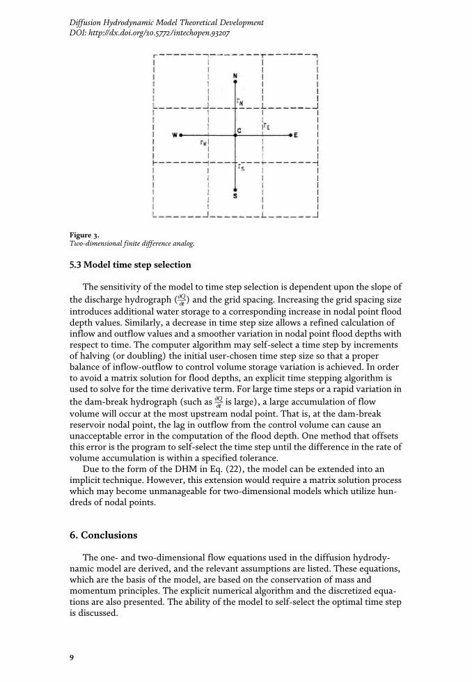
For uniform grid elements, the integrated finite difference version of the nodaldomain integration (NDI) method [6] is used. For grid elements, the NDI nodalequation is based on the usual nodal system shown in Figure 3. Flow rates across theboundary Г are estimated by assuming a linear trial function between nodal points.
For a square grid of width δ
q ГEj ¼ � KX ГEj½ � HE �HC½ �∕δ (34)
where
KxjГE
1:486n
h5=3� �
ГE
. HE �HC
δ cos θ
��������1=2
; jHE �Hcj≥ℇ
0 ; HE �HCj j< ε
8><>:
(35)
In Eq. (35), h (depth of water) and n (the Manning’s coefficient) are both theaverage of their respective values at C and E, i.e., h ¼ hC þ hEð Þ=2 and n ¼nC þ nEð Þ=2. Additionally, the denominator of KX is checked such that KX is set tozero if HE �HCj j is less than a tolerance ε such as 10�3 ft.
The net volume of water in each grid element between time step i and i + 1 isΔqC
i ¼ q rEj þ q rwj þ q rNj þ q rSj and the change of depth of water is ΔHCi ¼
ΔqCi ∗Δt=δ2 for time step i and i + 1 with Δt interval. Then the model advances in
time by an explicit approach
HCiþ1 ¼ ΔHC
i þHCi (36)
where the assumed input flood flows are added to the specified input nodes ateach time step. After each time step, the hydraulic conductivity parameters ofEq. (35) are reevaluated, and the solution of Eq. (36) is reinitiated.
8
A Diffusion Hydrodynamic Model
5.3 Model time step selection
The sensitivity of the model to time step selection is dependent upon the slope ofthe discharge hydrograph (∂Q
∂t ) and the grid spacing. Increasing the grid spacing sizeintroduces additional water storage to a corresponding increase in nodal point flooddepth values. Similarly, a decrease in time step size allows a refined calculation ofinflow and outflow values and a smoother variation in nodal point flood depths withrespect to time. The computer algorithm may self-select a time step by incrementsof halving (or doubling) the initial user-chosen time step size so that a properbalance of inflow-outflow to control volume storage variation is achieved. In orderto avoid a matrix solution for flood depths, an explicit time stepping algorithm isused to solve for the time derivative term. For large time steps or a rapid variation inthe dam-break hydrograph (such as ∂Q
∂t is large), a large accumulation of flowvolume will occur at the most upstream nodal point. That is, at the dam-breakreservoir nodal point, the lag in outflow from the control volume can cause anunacceptable error in the computation of the flood depth. One method that offsetsthis error is the program to self-select the time step until the difference in the rate ofvolume accumulation is within a specified tolerance.
Due to the form of the DHM in Eq. (22), the model can be extended into animplicit technique. However, this extension would require a matrix solution processwhich may become unmanageable for two-dimensional models which utilize hun-dreds of nodal points.
6. Conclusions
The one- and two-dimensional flow equations used in the diffusion hydrody-namic model are derived, and the relevant assumptions are listed. These equations,which are the basis of the model, are based on the conservation of mass andmomentum principles. The explicit numerical algorithm and the discretized equa-tions are also presented. The ability of the model to self-select the optimal time stepis discussed.
Figure 3.Two-dimensional finite difference analog.
9
Diffusion Hydrodynamic Model Theoretical DevelopmentDOI: http://dx.doi.org/10.5772/intechopen.93207
elevation, and initial flow depth (usually zero) are assigned. With these initialconditions, the solution is advanced to the next time step (t + Δt) as detailed below
1.Between nodal points, compute an average Manning’s n and average geometricfactors
2.Assuming mX = 0, estimate the nodal flow depths for the next time step(t + Δt) by using Eqs. (20) and (21) explicitly
3.Using the flow depths at time t and t + Δt, estimate the mid time step value ofmX selected from Eq. (23)
4.Recalculate the conductivities KX using the appropriate mX values
5.Determine the new nodal flow depths at the time (t + Δt) using Eq. (19), and
6.Return to step (3) until KX matches mid time step estimates.
The above algorithm steps can be used regardless of the choice of definition formX from Eq. (23). Additionally, the above program steps can be directly applied to atwo-dimensional diffusion model with the selected (mX,my) relations incorporated.
5.2 Numerical model formulation (grid element)
For uniform grid elements, the integrated finite difference version of the nodaldomain integration (NDI) method [6] is used. For grid elements, the NDI nodalequation is based on the usual nodal system shown in Figure 3. Flow rates across theboundary Г are estimated by assuming a linear trial function between nodal points.
For a square grid of width δ
q ГEj ¼ � KX ГEj½ � HE �HC½ �∕δ (34)
where
KxjГE
1:486n
h5=3� �
ГE
. HE �HC
δ cos θ
��������1=2
; jHE �Hcj≥ℇ
0 ; HE �HCj j< ε
8><>:
(35)
In Eq. (35), h (depth of water) and n (the Manning’s coefficient) are both theaverage of their respective values at C and E, i.e., h ¼ hC þ hEð Þ=2 and n ¼nC þ nEð Þ=2. Additionally, the denominator of KX is checked such that KX is set tozero if HE �HCj j is less than a tolerance ε such as 10�3 ft.
The net volume of water in each grid element between time step i and i + 1 isΔqC
i ¼ q rEj þ q rwj þ q rNj þ q rSj and the change of depth of water is ΔHCi ¼
ΔqCi ∗Δt=δ2 for time step i and i + 1 with Δt interval. Then the model advances in
time by an explicit approach
HCiþ1 ¼ ΔHC
i þHCi (36)
where the assumed input flood flows are added to the specified input nodes ateach time step. After each time step, the hydraulic conductivity parameters ofEq. (35) are reevaluated, and the solution of Eq. (36) is reinitiated.
8
A Diffusion Hydrodynamic Model
5.3 Model time step selection
The sensitivity of the model to time step selection is dependent upon the slope ofthe discharge hydrograph (∂Q
∂t ) and the grid spacing. Increasing the grid spacing sizeintroduces additional water storage to a corresponding increase in nodal point flooddepth values. Similarly, a decrease in time step size allows a refined calculation ofinflow and outflow values and a smoother variation in nodal point flood depths withrespect to time. The computer algorithm may self-select a time step by incrementsof halving (or doubling) the initial user-chosen time step size so that a properbalance of inflow-outflow to control volume storage variation is achieved. In orderto avoid a matrix solution for flood depths, an explicit time stepping algorithm isused to solve for the time derivative term. For large time steps or a rapid variation inthe dam-break hydrograph (such as ∂Q
∂t is large), a large accumulation of flowvolume will occur at the most upstream nodal point. That is, at the dam-breakreservoir nodal point, the lag in outflow from the control volume can cause anunacceptable error in the computation of the flood depth. One method that offsetsthis error is the program to self-select the time step until the difference in the rate ofvolume accumulation is within a specified tolerance.
Due to the form of the DHM in Eq. (22), the model can be extended into animplicit technique. However, this extension would require a matrix solution processwhich may become unmanageable for two-dimensional models which utilize hun-dreds of nodal points.
6. Conclusions
The one- and two-dimensional flow equations used in the diffusion hydrody-namic model are derived, and the relevant assumptions are listed. These equations,which are the basis of the model, are based on the conservation of mass andmomentum principles. The explicit numerical algorithm and the discretized equa-tions are also presented. The ability of the model to self-select the optimal time stepis discussed.
Figure 3.Two-dimensional finite difference analog.
9
Diffusion Hydrodynamic Model Theoretical DevelopmentDOI: http://dx.doi.org/10.5772/intechopen.93207

Author details
Theodore V. Hromadka II1* and Chung-Cheng Yen2
1 Department of Mathematical Sciences, United States Military Academy,West Point, NY, USA
2 Tetra Tech, Irvine, CA, USA
*Address all correspondence to: [email protected]
©2020TheAuthor(s). Licensee IntechOpen.Distributed under the terms of theCreativeCommonsAttribution -NonCommercial 4.0 License (https://creativecommons.org/licenses/by-nc/4.0/),which permits use, distribution and reproduction fornon-commercial purposes, provided the original is properly cited. –NC
10
A Diffusion Hydrodynamic Model
References
[1] Akan AO, Yen BC. Diffusion-waveflood routing in channel networks.ASCE Journal of Hydraulic Division.1981;107(6):719-732
[2] Hromadka TV II, Berenbrokc CE,Freckleton JR, Guymon GL. A two-dimensional diffusion dam-breakmodel. Advances in Water Resources.1985;8:7-14
[3] Xanthopoulos TH, Koutitas CH.Numerical simulation of a two-dimensional flood wave propagationdue to dam failure. ASCE Journal ofHydraulic Research. 1976;14(4):321-331
[4] Hromadka TV II, Lai C. Solving thetwo-dimensional diffusion flow model.In: Proceedings of ASCE HydraulicsDivision Specialty Conference, Orlando,Florida. 1985
[5] Hromadka TV II, Nestlinger AB.Using a two-dimensional diffusionaldam-break model in engineeringplanning. In: Proceedings of ASCEWorkshop on Urban Hydrology andStormwater Management, Los AngelesCounty Flood Control District Office,Los Angeles, California. 1985
[6] Hromadka TV II, Guymon GL,Pardoen G. Nodal domain integrationmodel of unsaturated two-dimensionalsoil water flow: Development. WaterResources Research. 1981;17:1425-1430
11
Diffusion Hydrodynamic Model Theoretical DevelopmentDOI: http://dx.doi.org/10.5772/intechopen.93207

13
Chapter 2
Verification of Diffusion Hydrodynamic ModelTheodore V. Hromadka II and Chung-Cheng Yen
Abstract
The efficacy of the one- and two-dimensional diffusion hydrodynamic model (DHM) for predicting flow characteristics resulting from a dam-break scenario is tested. The model results, for different inflow scenarios, are compared with the standard United States Geological Survey (USGS) K-634 model. The sensitivity of the model results to grid spacing and the chosen time step are presented. The model results are in close agreement.
Keywords: floodplain, hydrograph, unsteady flows, initial flow condition, spatial grid size, transient simulation
1. Introduction
An unsteady flow hydraulic problem of considerable interest is the analysis of dam breaks and their downstream hydrograph. In this section, the main objective is to evaluate the diffusion form of the flow equations for the estimation of flood depths (and the floodplain), resulting from a specified dam-break hydrograph. The dam-break failure mode is not considered in this section. Rather, the dam-break failure mode may be included as part of the model solution (such as for a sudden breach) or specified as a reservoir outflow hydrograph.
The use of numerical methods to approximately solve the flow equations for the propagation of a flood wave due to an earthen dam failure has been the subject of several studies reported in the literature. Generally, the flow is modeled using the one-dimensional equation wherever there is no significant lateral variation in the flow. Land [1, 2] examined four such dam-break models in his prediction of flood-ing levels and flood wave travel time and compares the results against observed dam failure information. In the dam-break analysis, an assumed dam-break failure mode (which may be part of the solution) is used to develop an inflow hydrograph to the downstream floodplain. Consequently, it is noted that a considerable sensitivity in modeling results is attributed to the dam-break failure rate assumptions. Ponce and Tsivoglou [3] examined the gradual failure of an earthen embankment (caused by an overtopping flooding event) and present detailed analysis for each part of the total system: sediment transport, unsteady channel hydraulics, and earth embank-ment failure.
In another study, Rajar [4] studied a one-dimensional flood wave propagation from an earthen dam failure. His model solved the St. Venant equations using either a first-order diffusive or a second-order Lax-Wendroff numerical scheme. A review of the literature indicates that the most frequently used numerical scheme was the

A Diffusion Hydrodynamic Model
14
method of characteristics (to solve the governing flow equations) as described in Sakkas and Strelkoff [5], Chen [6], and Chen and Armbruster [7].
Although many dam-break studies involve flood flow regimes which are truly two-dimensional (in the horizontal plane), the two-dimensional case has not received much attention in the literature. Katopodes and Strelkoff [8] used the method of bicharacteristics to solve the governing equations of continuity and momentum. The model utilizes a moving grid algorithm to follow the flood wave propagation and also employs several interpolation schemes to approximate the nonlinearity effects. In a much simpler approach, Xanthopoulos and Koutitas [9] used a diffusion model (i.e., the inertial terms are assumed negligible in comparison to the pressure, friction, and gravity components) to approximate a two-dimen-sional flow field. The model assumed that the flow regime in the floodplain is such that the inertial terms (local and convective acceleration) are negligible. In a one-dimensional model, Akan and Yen [10] also used the diffusion approach to model hydrograph confluences at channel junctions. In the latter study, comparisons of modeling results were made between the diffusion model, a complete dynamic wave model solving the total equation system, and the basic kinematic-wave equation model (i.e., the inertia and pressure terms are assumed negligible in comparison to the friction and gravity terms). The differences between the diffusion model and the dynamic wave model were small, showing only minor discrepancies.
The kinematic-wave flow model has been used in the computation of dam-break flood waves [11]. Hunt concluded in his study that the kinematic-wave solution is asymptotically valid. Since the diffusion model has a wider range of applicability for varied bed slopes and wave periods than the kinematic model [12], the diffusion model approach should provide an extension to the referenced kinematic model.
Because the diffusion modeling approach leads to an economic two-dimensional dam-break flow model (with numerical solutions based on the usual integrated finite difference or finite element techniques), the need to include the extra compo-nents in the momentum equation must be ascertained. For example, evaluating the convective acceleration terms in a two-dimensional flow model requires approxi-mately an additional 50 percent of the computational effort required in solving the entire two-dimensional model with the inertial terms omitted. Consequently, including the local and convective acceleration terms increases the computer execution costs significantly. Such increases in computational effort may not be significant for one-dimensional case studies; however, two-dimensional case stud-ies necessarily involve considerably more computational effort, and any justifiable simplifications of the governing flow equations is reflected by a significant decrease in computer software requirements, costs, and computer execution time.
Ponce [13] examined the mathematical expressions of the flow equations, which lead to wave attenuation in prismatic channels. It is concluded that the wave attenuation process is caused by the interaction of the local acceleration term with the sum of the terms of friction slope and channel slope. When local acceleration is considered negligible, wave attenuation is caused by the interaction of the friction slope and channel slope terms with the pressure gradient or convective acceleration terms (or a combination of both terms). Other discussions of flow conditions and the sensitivity to the various terms of the flow equations are given in Miller and Cunge [14], Morris and Woolhiser [15], and Henderson [16].
It is stressed that the ultimate objective of this effort is to develop a two-dimen-sional diffusion model for use in estimating floodplain evolution, such as those that occur due to drainage system deficiencies. Prior to finalizing such a model, the requirement of including the inertial terms in the unsteady flow equations needs to be ascertained. The strategy used to check on this requirement is to evaluate the accuracy in predicted flood depths produced from a one-dimensional diffusion
15
Verification of Diffusion Hydrodynamic ModelDOI: http://dx.doi.org/10.5772/intechopen.93208
model with respect to the one-dimensional United States Geological Survey (USGS) K-634 dam-break model which includes all of the inertial term components.
2. One-dimensional analysis
2.1 Study approach
To evaluate the accuracy of the one-dimensional diffusion model [Chapter 1, Eq. 22) in the prediction of flood depths, the USGS fully dynamic flow model K-634 [1, 2] is used to determine channel flood depths for comparison purposes. The K-634 model solves the coupled flow equations of continuity and momen-tum by an implicit finite difference approach and is considered to be a highly accurate model for many unsteady flow problems. The study approach is to compare predicted (1) flood depths and (2) discharge hydrographs from both the K-634 and the diffusion hydrodynamic model (DHM) for various channel slopes and inflow hydrographs.
It should be noted that different initial conditions are used for these two models. The USGS K-634 model requires a base flow to start the simulation; therefore, the initial depth of water cannot be zero. Next, the normal depth assumption is used to generate an initial water depth before the simulation starts. These two steps are not required by the DHM.
In this case study, two hydrographs are assumed; namely, peak flows to 120,000 and 600,000 cfs. A base flow of 5000 and 40,000 cfs was used for hydrographs with peaks of 120,000 and 600,000 cfs, respectively, for all K-634 simulations. Both hydrographs are assumed to increase linearly from zero (or the base flow) to the peak flow rate at 1 h and then decrease linearly to zero (or the base flow) at 6 h (see Figure 1 inset). The study channel is assumed to be a 1000-feet-width rectangular section of Manning’s n equal to 0.040 and various slopes S0 in the range of 0.001 ≤ S0 ≤ 0.01. Figure 1 shows the comparison of modeling results. From the figure, various flood depths are plotted along the channel length of up to 10 miles. Two reaches of channel lengths of up to 30 miles are also plotted in Figure 1 which correspond to a slope S0 = 0.0020. In all tests, grid spacing was set at 1000-feet intervals. Time steps were 0.01 h for K-634 and 7.2 s for DHM.
From Figure 1, it is seen that the diffusion model provides estimates of flood depths that compare very well to the flood depths predicted from the K-634 model. For downstream distances at up to 30 miles, differences in predicted flood depths are less than 3% for the various channel slopes and peak flow rates considered.
In Figures 2–5, good comparisons between the diffusion hydrodynamic and the K-634 models are observed for water depths and outflow hydrographs at 5 and 10 miles downstream from the dam-break site. It should be noted that the test conditions are purposefully severe in order to bring out potential inaccuracies in the diffusion hydrodynamic model results. Less severe test conditions should lead to more favorable comparisons between the two model results. Although offsets do occur in timing, volume continuity is preserved when allowances are made for differences in base flow volumes.
2.2 Grid spacing selection
The choice of the time step and grid size for an explicit time advancement is a relative matter and is theoretically based on the well-known Courant condition [17]. The choice of grid size usually depends on available topographic data for nodal elevation determination and the size of the problem. The effect of the grid size

A Diffusion Hydrodynamic Model
16
(for constant time step for 7.2 s) on the diffusion model accuracy can be shown by example where nodal spacings of 1000, 2000, and 5000 feet are considered. The predicted flood depths varied only slightly from choosing the grid size between 1000 and 2000 feet. However, an increased variation in results occurs when a grid size of 5000 feet is selected. For the example of peak flow rate test hydrograph of 600,000 cfs, the differences of simulated flow depths between 1000 and 5000-feet grid are 0.03, 0.06, and 0.17 feet at 1, 5, and 10 miles, respectively, downstream from the dam-break site for the maximum flow depth with the magnitude of 30 feet.
Because the algorithm presented is based upon an explicit time stepping tech-nique, the modeling results may become inaccurate, should the time step size versus grid size ratio become large. A simple procedure to eliminate this instability is to half the time step size until convergence in computed results is achieved. Generally,
Figure 1. Diffusion hydrodynamic model and K-634 model results (solid line) for 1000-feet-width channel, Manning’s n = 0.040, and various channel slopes, S0.
17
Verification of Diffusion Hydrodynamic ModelDOI: http://dx.doi.org/10.5772/intechopen.93208
such a time step adjustment may be directly included in the computer program for the dam-break model. For the cases considered in this section, the time step size of 7.2 s was found to be adequate when using the 1000–5000-feet grid sizes.
Figure 2. Comparisons of outflow hydrographs at 5 and 10 miles downstream from the dam – break site (peak Q = 120,000 cfs) (A) S = 0.001 (B) S = 0.008.
Figure 3. Comparisons of outflow hydrographs at 5 and 10 miles downstream from the dam – break site (peak Q = 600,000 cfs) (C) S = 0.001 (D) S = 0.008.

A Diffusion Hydrodynamic Model
18
2.3 Results
For the dam-break hydrographs considered and the range of channel slopes modeled, the simple diffusion dam-break model of Eq. (22) in Chapter 1 provides estimates of flood depths and outflow hydrographs which compare favorably to the results determined by the well-known K-634 one-dimensional dam-break model. Generally speaking, the difference between the two modeling approaches is found to be less than a 3% variation in predicted flood depths.
Figure 4. Comparisons of depths of water at (A) 5 miles and (B) 10 miles downstream from the dam-break site (peak Q = 120,000 cfs).
19
Verification of Diffusion Hydrodynamic ModelDOI: http://dx.doi.org/10.5772/intechopen.93208
The presented diffusion dam-break model is based upon a straightforward explicit time stepping method which allows the model to operate upon the nodal points without the need to use large matrix systems. Consequently, the model can be implemented on most currently available microcomputers. However, as com-pared to implicit solution methods, time steps for DHM use are extremely small. Thus, relatively short simulation times must be used.
The diffusion model of Eq. (22) in Chapter 1 can be directly extended to a two-dimensional model by adding the y-direction terms, which are computed in a similar fashion as the x-direction terms. The resulting two-dimensional diffusion
Figure 5. Comparisons of depths of water at (C) 5 miles and (D) 10 miles downstream from the dam-break site (peak Q = 600,000 cfs).

A Diffusion Hydrodynamic Model
20
model is texted by modeling the considered test problems in the x-direction, the y-direction, and along a 45-degree trajectory across a two-dimensional grid aligned with the x-y coordinate axis. Using a similar two-dimensional model, Xanthopoulos and Koutitas [9] conceptually verify the diffusion modeling technique by consider-ing the evolution of a two-dimensional floodplain which propagates radially from the dam-break site.
From the above conclusions, the use of the diffusion approach (Chapter 1, Eq. 22), in a two-dimensional DHM may be justified due to the low variation in predicted flooding depths (one-dimensional) with the exclusion of the inertial terms. Generally speaking, a two-dimensional model would be employed when the expansion nature of flood flows is anticipated. Otherwise, one of the available one-dimensional models would suffice for the analysis.
3. Two-dimensional analysis
3.1 Introduction
In this section, a two-dimensional DHM is developed. The model is based on a diffusion approach where gravity, friction, and pressure forces are assumed to dom-inate the flow equations. Such an approach has been used earlier by Xanthopoulos and Koutitas [9] in the prediction of dam-break floodplains in Greece. In those studies, good results were also obtained by using the two-dimensional model for predicting one-dimensional flow quantities. In the preceding section, a one-dimen-sional diffusion model has been considered, and it has been concluded that for most velocity flow regimes (such as Froude number less than approximately 4), the diffu-sion model is a reasonable approximation of the full dynamic wave formulation.
An integrated finite difference grid model is developed which equates each cell-centered node to a function of the four neighboring cell nodal points. To demon-strate the predictive capacity of the floodplain model, a study of a hypothetical dam break of the Crowley Lake dam near the city of Bishop, California (Figure 6), is considered [18, 19].
The steepness and confinement of the channel right beneath the Crowley Lake dam results in a translation of outflow hydrograph in time. Therefore, the dam-break analysis is only conducted in the neighborhood near the city of Bishop, where the gradient of topography is mild.
3.2 K-634 modeling results and discussion
Using the K-634 model for computing the two-dimensional flow was attempted by means of the one-dimensional nodal spacing (Figure 7). Cross sections were obtained by field survey, and the elevation data were used to construct nodal point flow-width versus stage diagrams. A constant Manning’s roughness coefficient of 0.04 was assumed for study purposes. The assumed dam failure reached a peak flow rate of 420,000 cfs within 1 h and returned to zero flow 9.67 h later. Figure 8 depicts the K-634 floodplain limits. To model the flow breakout, a slight gradient was assumed for the topography perpendicular to the main channel. The motiva-tion for such a lateral gradient is to limit the channel flood-way section in order to approximately conserve the one-dimensional momentum equations. Consequently, fictitious channel sides are included in the K-634 model study, which results in artificial confinement of the flows. Hence, a narrower floodplain is delineated in Figure 8 where the flood flows are falsely retained within a hypothetical channel confine. An examination of the flood depths given in Figure 9 indicates that at
21
Verification of Diffusion Hydrodynamic ModelDOI: http://dx.doi.org/10.5772/intechopen.93208
the widest floodplain expanse of Figure 8, the flood depth is about 6 feet, yet the floodplain is not delineated to expand southerly but is modeled to terminate based on the assumed gradient of the topography toward the channel. Such complications in accommodating an expanding floodplain when using a one-dimensional model are obviously avoided by using a two-dimensional approach.
The two-dimensional diffusion hydrodynamic model is now applied to the hypo-thetical dam-break problem using the grid discretization shown in Figure 10. The same
Figure 6. Dam-break study location.
Figure 7. Surveyed cross section locations on Owens River for use in K-634 model.

A Diffusion Hydrodynamic Model
22
inflow hydrograph used in K-634 model is also used for the diffusion hydrodynamic model. Again, Manning’s roughness coefficient at 0.04 was used. The resulting flood-plain is shown in Figure 11 for the 1/4 square-mile grid model.
The two approaches are comparable except at cross sections shown as A-A and B-B in Figure 7. Cross section A-A corresponds to the predicted breakout of flows
Figure 8. Floodplain computed from K-634 model.
Figure 9. Comparison of modeled water surface elevations (Points A and B in the figure are selected as example locations where a greater than an average difference between tested model predictions are observed).
23
Verification of Diffusion Hydrodynamic ModelDOI: http://dx.doi.org/10.5772/intechopen.93208
away from the Owens River channel with flows traveling southerly toward the city of Bishop. As discussed previously, the K-634 predicted flood depth corresponds to a flow depth of 6 feet (above natural ground) which is actually unconfined by the channel. The natural topography will not support such a flood depth, and,
Figure 10. Floodplain discretization for two-dimensional diffusion hydrodynamic model.
Figure 11. Floodplain for two-dimensional diffusion hydrodynamic model.
A Diffusion Hydrodynamic Model
24
Author details
Theodore V. Hromadka II 1* and Chung-Cheng Yen2
1 Department of Mathematical Sciences, United States Military Academy, West Point, NY, USA
2 Tetra Tech, Irvine, CA, USA
*Address all correspondence to: [email protected]
consequently, there should be southerly breakout flows such as predicted by the two-dimensional model. With such breakout flows included, it is reasonable that the two-dimensional model would predict a lower flow depth at cross section A-A.
At cross section B-B, the K-634 model predicts a flood depth of approximately 2 feet less than the two-dimensional model. However, at this location, the K-634 modeling results are based on cross sections, which traverse a 90-degree bend. In this case K-634 model will overestimate the true channel storage, resulting in an underestimation of flow depths.
4. Conclusions
The contribution of inertial terms for one-dimensional flows resulting from a dam break was investigated by comparing the results of the DHM with the K-634 model, which includes inertial terms. The close agreement between the two models predicted results justifies the use of the DHM for these applications.
For two-dimensional flows, comparing the various model predicted flood depths and delineated plains, it is seen that the two-dimensional diffusion hydrody-namic model predicted more reasonable floodplain boundary, which is associated with broad, flat plains such as those found at the study site. The model approxi-mates channel bends, channel expansions and contractions, flow breakouts, and the general area of inundation. Additionally, the diffusion hydrodynamic model approach allows for the inclusion of return flows (to the main channel), which were the result of upstream channel breakout, and other two-dimensional flow effects, without the need for special modeling accommodations that would be necessary with using a one-dimensional model.
© 2020 The Author(s). Licensee IntechOpen. Distributed under the terms of the Creative Commons Attribution - NonCommercial 4.0 License (https://creativecommons.org/licenses/by-nc/4.0/), which permits use, distribution and reproduction for non-commercial purposes, provided the original is properly cited.
25
Verification of Diffusion Hydrodynamic ModelDOI: http://dx.doi.org/10.5772/intechopen.93208
[1] Land LF. Mathematical simulations of the Toccoa Falls, Georgia, Dam-Break Flood. Water Resources Bulletin. 1980;16(6):1041-1048
[2] Land LF. Evaluation of selected dam-break flood-wave models by using field data. U.S.G.S. Water Resources Investigations. 1980;80(4):54
[3] Ponce VM, Tsivoglou AJ. Modeling gradual dam breaches. ASCE Journal of Hydrauic Division. 1981;107(7):829-838
[4] Rajar R. Mathematical simulation of dam-break flow. ASCE Journal of Hydrauic Division. 1978;104(7):1011-1026
[5] Sakkas JG, Strelkoff T. Dam-break flood in a prismatic dry channel. ASCE Journal of Hydrauic Division. 1973;99(12):2195-2216
[6] Chen C. Laboratory verification of a dam-break flood model. ASCE Journal of Hydrauic Division. 1980;106(4):535-556
[7] Chen C, Armbruster JT. Dam-break wave model: Formulation and verification. ASCE Journal of Hydrauic Division. 1980;106(5):747-767
[8] Katopodes N, Strelkoff T. Computing two-dimensional dam-break flood waves. ASCE Journal of Hydrauic Division. 1978;104(9):1269-1288
[9] Xanthopoulos T, Koutitas C. Numerical simulation of a two-dimensional flood wave propagation due to dam failure. ASCE Journal of Hydraulic Research. 1976;14(4):321-331
[10] Akan AO, Yen BC. Diffusion-wave flood routing in channel networks. ASCE Journal of Hydrauic Division. 1981;107(6):719-732
[11] Hunt T. Asymptotic solution for dam-break problem. ASCE Journal of Hydrauic Division. 1982;108(1):115-126
[12] Ponce VM, Li RM, Simons DB. Applicability of kinematic and diffusion models, in verification of mathematical and physical models in hydraulic engineering. In: American Society of Civil Engineers, Hydraulic Division, Special Conference College Park, Maryland: University of Maryland; 1978. pp. 605-613
[13] Ponce VM. Nature of wave attenuation in Open Channel flow. ASCE Journal of Hydrauic Division. 1982;108(2):257-262
[14] Miller WA, Cunge JA. Simplified Equations of Unsteady Flow. Chapter 5 of Unsteady Flow in Open Channels. Vol. 1. Fort Collins, Colorado: Water Resources Publications; 1975. pp. 183-257
[15] Morris EM, Woolhiser DA. Unsteady one-dimensional flow over a plane: Partial equilibrium and recession hydrographs. Water Resources Research, AGU. 1980;16(2):356-360
[16] Henderson FM. Flood waves in prismatic channels. ASCE Journal of Hydrauic Division. 1963;89(4):39-67
[17] Basco DR. Introduction to numerical method—Part I and II. Verification of mathematical and physical models in hydraulic engineering. In: American Society of Civil Engineers, Hydraulic Division, Special Conference College Park, Maryland: University of Maryland; 1978. pp. 280-302
[18] Hromadka II TV, Lai C. Solving the two-dimensional diffusion flow model. In: Proceedings of ASCE Hydraulics Division Specialty Conference, Orlando, Florida. 1985
References

A Diffusion Hydrodynamic Model
26
[19] Hromadka II TV, Nestlinger AB. Using a two-dimensional diffusional dam-break model in engineering planning. In: Proceedings of ASCE Workshop on Urban Hydrology and Stormwater Management, Los Angeles County Flood Control District Office, Los Angeles, California. 1985
27
Chapter 3
Program Description of the Diffusion Hydrodynamic ModelTheodore V. Hromadka II and Chung-Cheng Yen
Abstract
The numerical algorithm, with a focus on the interface element that is used in the diffusion hydrodynamic model, is presented in this chapter. The source program was written in FORTRAN language, and it can be downloaded from this book companion website. The channel, flood plain, and the interface flow details are discussed.
Keywords: flood plain, overflow, control volume, water elevation, channel interface
1. Introduction
A computer program for the two-dimensional diffusion hydrodynamic model which is based on the diffusion form of the St. Venant equations [1–5] where grav-ity, friction, and pressure forces are assumed to dominate the flow equation will be discussed in this section.
The DHM consists of a 1-D channel and 2-D flood plain models, and an inter-face sub-model. The one-dimensional channel element utilizes the following assumptions:
• Infinite vertical extensions on channel walls (Figure 1)
• Wetted perimeter is calculated as shown in Figure 1(a)
• Volumes due to channel skew are ignored (Figure 1(b))
• All overflow water is assigned to one grid element (Figure 2)
The interface model calculates the excess amount of water either from the channel element or from the flood plain element. This excess water is redistributed to the flood plain element or the channel element according to the water surface elevation.
This FORTRAN program has the capabilities to simulate both one-and two-dimensional surface flow problems, such as the one-dimensional open channel flow and two-dimensional dam-break problems illustrated in the preceding pages. Engineering applications of the program will be presented in the next chapter.

A Diffusion Hydrodynamic Model
28
2. Interface model
2.1 Introduction
The interface model modifies the water surface elevations of flood plain grids and channel elements at specified time intervals (update intervals). There are three cases of interface situations: (1) channel overflow, (2) grid overflow, and (3) flood-ing of channel and grid elements.
Figure 1. One-dimensional channel flow element characteristics: (a) element geometrics, (b) element associations to grid elements, and (c) channel element connections.
29
Program Description of the Diffusion Hydrodynamic ModelDOI: http://dx.doi.org/10.5772/intechopen.93209
2.2 Channel overflow
When the channel is overflowing; the excess water is temporarily stored in the vertically extended space (Figure 3(b)). Actually, it is the volume per unit length. This excess water is the product of the depth of water, the width of the channel, and the length of the channel and is subsequently uniformly distributed over the grid elements. In other words, the new grid water surface elevation is equal to the old water surface elevation plus a depth of hw/L, and the channel water surface elevation now matches the parent grid water surface elevation.
2.3 Grid overflow
When the water surface elevation of the grid element is greater than a speci-fied surface detention (Figure 3(a)), the excess water drains into the channel element, and the new water surface elevation is changed according to the follow-ing two conditions (Figure 3(c)), (a) if v > v’, where v denotes the excess volume of water per unit length and v’ denotes the available volume per unit length, the new water surface of the grid element is ANEW = AOLD − (v − v’)/L, and the new water surface elevation of the channel element is also equal to ANEW, and (b) if v ≤ v’, the new water surface elevation of the grid element is ANEW = AOLD − h and the new water surface elevation of the channel element is BNEW = BOLD + v/w.
Figure 2. Grid element nodal molecule.

A Diffusion Hydrodynamic Model
30
Figure 3. Diffusion hydrodynamic interface model: (a) model interface geometries, (b) channel overflow interface model, (c) grid overflow interface model, (d) grid-channel flooding interface model, and (e) channel-grid flooding interface model.
31
Program Description of the Diffusion Hydrodynamic ModelDOI: http://dx.doi.org/10.5772/intechopen.93209
Author details
Theodore V. Hromadka II 1* and Chung-Cheng Yen2
1 Department of Mathematical Sciences, United States Military Academy, West Point, NY, USA
2 Tetra Tech, Irvine, CA, USA
*Address all correspondence to: [email protected]
2.4 Flooding of channel and grid
When flooding occurs, the water surface elevations of the grid and channel elements are both greater than the specified surface detention elevation. Two cases have to be considered as follows:
1. If A > B (Figure 3(d)), the new water surface elevation of the grid element is ( ) OLDNEW h L w
BL
A-
+= , and the new water surface elevation of the channel
element is equal to ANEW.
2. If A < B (Figure 3(e)), the new water surface elevation of the grid element is * NEW OLD h w
A AL
+= , and the new water surface elevation of the channel element
is equal to ANEW.
3. Conclusions
The characteristic features of the diffusion hydrodynamic model are detailed with a focus on its ability to model the interface. The interface component in the model can modify the water elevation in the grids along the flood plain and channel to account for different overflow scenarios, which are also illustrated.
© 2020 The Author(s). Licensee IntechOpen. Distributed under the terms of the Creative Commons Attribution - NonCommercial 4.0 License (https://creativecommons.org/licenses/by-nc/4.0/), which permits use, distribution and reproduction for non-commercial purposes, provided the original is properly cited.

32
A Diffusion Hydrodynamic Model
References
[1] Abbott MB, Bathurst JC, Cunge JA, O’Connell PE, Rasmussen J. An introduction to the European hydrological system—Système Hydrologique Européen, “SHE”, 1: History and philosophy of a physically based distributed modeling system. Journal of Hydrology. 1986;87(1-2):45-59
[2] Amein M, Fang CS. Implicit flood routing in natural channels. Journal of Hydraulics Division, Proceedings of ASCE. 1970;96(12):2481-2500
[3] Balloffet A, Scheffler ML. Numerical analysis of the Teton dam failure flood. Journal of Hydraulic Research. 1982;20(4):317-328
[4] Borah DK, Prasad SN, Alonso CV. Kinematic wave routing incorporating shock fitting. Water Resources Research. 1980;16(3):529-541
[5] Li RM, Simons DB, Stevens MA. Nonlinear kinematic wave approxi-mation for water routing. Water Resources Research. 1975;11(2):245-252
Chapter 4
Applications of DiffusionHydrodynamic ModelTheodore V. Hromadka II and Chung-Cheng Yen
Abstract
The diffusion hydrodynamic model is applied for seven engineering applicationsthat are commonly encountered in real-world applications. Of the seven applica-tions, six relate to two-dimensional flows. The results are compared to other modelresults, where available. The results underscore the reliability of the DHM alongwith its limitation for modeling rapidly varying flows.
Keywords: hydraulic jump, hydrograph, two-dimensional flows, estuary,channel flood plain interface
1. One-dimensional model application
1.1 Application 1: steady flow in an open channel
Because the DHM is anticipated for use in modeling watershed phenomena, it isimportant that the channel models represent known flow characteristics. Unsteadyflow is examined in the previous section. For steady flow, a steady-state, graduallyvaried flow problem is simulated by the 2-D diffusion model. Figure 1 depicts boththe water levels form the 2-D diffusion model and from the gradually varied flowequation. For an 8000 cfs constant inflow rate, the water surface profiles from boththe 2-D diffusion model and the gradually varied flow equation match quite well.The discrepancies of these profiles occur at the breakpoints where the upstreamchannel slope and downstream channel slope change. At the first break point wherethe upstream channel slope is equal to 0.001 and the downstream channel slope isequal to 0.005, the water surface level is assumed to be equal to the critical depth.However, Henderson [1] notes that brink flow is typically less than the criticaldepth (Dc). The DHM water surface closely matches the 0.72 Dc brink depth.
It is clear to see that the DHM cannot simulate the hydraulic jump but rathersmooth out the usually assumed “shock front.” However, when consideringunsteady flow, the DHMmay be a reasonable approach for approximating the jumpprofile. For a higher inflow rate, 20,000 cfs, the surface water levels differ in themost upstream reach. Again, this is due to the downstream control, critical depth, ofthe gradually varied flow equation.
33

2. Two-dimensional model applications
2.1 Application 2: rainfall-runoff model
The DHM can be used to develop a runoff hydrograph given the time distribu-tion of effective rainfall. To demonstrate the DHM runoff hydrograph generation[2], the DHM is used to develop a synthetic S-graph for a watershed where theoverland flow is the dominating flow effect.
To develop the S-graph, a uniform effective rainfall is assumed to uniformlyoccur over the watershed. For each time step (5 s), an incremental volume of wateris added directly to each grid element based on the assumed constant rainfallintensity, resulting in an equivalent increase in the nodal point depth of water.Runoff flows to the point of concentration according to the two-dimensionaldiffusion hydrodynamics model.
The 10 square mile Cucamonga Creek Watershed (California) is shown,discretized by 1000-foot grid elements, in Figure 2. A design storm (Figure 3) wasapplied to the watershed, and the resulting runoff hydrographs are depicted inFigure 4 for DHM and synthetic unit hydrograph method. From Figure 4, thediffusion model generates runoff quantities which are in good agreement with thevalues computed using a synthetic unit hydrograph method derived from streamgage data.
Next, the DHM is applied to three hypothetical dam failures in OrangeCounty, California (see Figure 5). In this application, the ability of DHM topredict flow characteristics in domains where flood flow patterns are affected byrailroad, the bridge under crossings, and other man-made obstacles to flow isillustrated.
Figure 1.Gradually varied flow profiles. (a) Q = 20,000 cfs, downstream slope = 0.0001 (b) Q = 8,000 cfs, downstreamslope = 0.0001 (c) Q = 8,000 cfs, downstream slope = 0.0002.
34
A Diffusion Hydrodynamic Model
Major assumptions used in these assumptions are as follows:
1.In each grid, an area-averaged ground elevation was estimated based on thetopographic map, and a Manning’s roughness coefficient was used for eachapplication.
2.All storm drain systems provide negligible draw off of the dam-break flows.This assumption accommodates a design storm in progress during the damfailure. This assumption also implies that stormwater runoff provides anegligible increase to the dam-break flow hydrograph.
3.All canyon damming effects due to culvert crossings provide negligibleattenuation of dam-break flows. This assumption is appropriate due to theconcurrent design storm assumption and due to sediment deposition from thetransport of the reservoir earthen dam materials.
4.The reservoir failure yields an outflow hydrograph, as depicted in Figure 6.
Figure 2.Cucamonga Creek discretization.
35
Applications of Diffusion Hydrodynamic ModelDOI: http://dx.doi.org/10.5772/intechopen.93210

2.2 Application 3: small dam-break floodplain analysis
A study of a hypothetical failure of the Orange Country Reservoir northeast ofthe city of Brea, California (Figure 7), was conducted by Hromadka and Lai [3].Using the USGS topographic quadrangle map (photo-revised, 1981), a 500-foot griddiscretization was prepared (Figure 8), and nodal-area ground elevations wereestimated based on the map. A Manning’s roughness coefficient of n = 0.040 wasused throughout the study, except in canyon reaches and grassy plains, where n wasselected as 0.030 and 0.050, respectively. In this study, the resulting flood plain andthe comparison of the model-simulated flood plain to a previous study by theMetropolitan Water District of Southern California [4] are shown in Figure 9. Themain difference in the estimated flood plains is due to the dynamic nature of the
Figure 3.Design storm for Cucamonga Creek.
36
A Diffusion Hydrodynamic Model
DHM, which accounts for the storage effects resulting from flooding, and theattenuation of a flood wave because of 2-D routing effects. From this study, theestimated flood plain is judged to be reasonable.
Figure 4.Simulated runoff hydrographs for Cucamonga Creek.
Figure 5.Vicinity map for dam-break analyses.
37
Applications of Diffusion Hydrodynamic ModelDOI: http://dx.doi.org/10.5772/intechopen.93210

Figure 6.Study dam-break outflow hydrograph for Orange County Reservoir.
Figure 7.Location map for the Orange County Reservoir dam-break problem.
38
A Diffusion Hydrodynamic Model
2.3 Application 4: small-scale flows onto a flat plain
A common civil engineering problem is the use of temporary detention basins tooffset the effects of urbanization on watershed runoff. A problem, however, is theanalysis of the basin failure, especially, when the flood flows enter a wide expanseof land surface with several small channels. This application is to present studyconclusions in estimating the flood plain, which may result from a hypotheticaldam failure of the LO2P3O temporary retarding basin. The results of this study areto be used to estimate the potential impacts of the area if the retention basin bermwere to fail.
The study site includes the area south of Plano Trabuco, Phase I. It isbounded on the north of LO2P3O Retarding Basin Berm, on the east and
Figure 8.Domain discretization for Orange County Reservoir.
39
Applications of Diffusion Hydrodynamic ModelDOI: http://dx.doi.org/10.5772/intechopen.93210

south of Portola Parkway, and on the west by the Arroyo Trabuco bluffs (seeFigure 10).
Using a 1″ = 3000 topographic map, a 200-foot grid control volume discretizationwas constructed, as shown in Figure 11. In each grid, an area-averaged groundelevation was estimated based on the topographic map. A Manning’s roughnesscoefficient of n = 0.030 was used throughout the study.
Figure 9.Comparison of flood plain results for Orange County Reservoir.
40
A Diffusion Hydrodynamic Model
The profile of Portola Parkway varies approximately 2 ft above and below theadjacent land. Consequently, minor ponding may occur where Portola Parkway ishigh and sheet flow across Portola Parkway will occur at low points. It should benoted that depths along Portola Parkway are less than 1 foot (Figure 11). Figure 12shows lines of arrival times for the basin study. It is concluded that Portola Parkwayis essentially unaffected by a hypothetical failure of the LO2P3O temporaryretarding basin.
2.4 Application 5: two-dimensional flood flows around a large obstruction
In another temporary detention basin site, flood flows (from a dam-break)would pond upstream of a landfill site, and then split, when waters are deepenough, to flow on either side of the landfill. An additional complication is arailroad berm located downstream of the landfill, which forms a channel for floodflows. The study site (see Figure 13) is bounded on the north by a temporary bermapproximately 300 ft north of the Union Pacific Railroad, bounded on the east byMilliken Avenue, bounded on the south by the Union Pacific Railroad, and boundedon the west by Haven Avenue.
Figure 10.Location map for L02P30 temporary retarding basin.
41
Applications of Diffusion Hydrodynamic ModelDOI: http://dx.doi.org/10.5772/intechopen.93210

A 200-foot grid control volume discretization was constructed as depicted inFigure 14. In each grid, an area-averaged ground elevation was estimated based onthe topographic map. A Manning’s roughness coefficient of n = 0.030 was usedthroughout the study.
Figure 11.Domain discretization of L02P30 temporary retarding basin.
Figure 12.Time of maximum flooding depth (80.5 acre—Feet basin test) for L02P30 temporary retarding basin.
42
A Diffusion Hydrodynamic Model
Figure 13.Location map for Ontario industrial partners’ temporary detention basin.
Figure 14.Domain discretization for Ontario industrial partners’ detention basin.
43
Applications of Diffusion Hydrodynamic ModelDOI: http://dx.doi.org/10.5772/intechopen.93210

From Figure 15, it is seen that flood plain spreads out laterally and flows aroundthe landfill. The flow ponds up around the landfill; along the north side of thelandfill, the water ponds as high as 9.2 ft, and along the east and west sides of the
Figure 15.Flood plain for Ontario industrial partners’ detention basin.
Figure 16.Time (h) of maximum flooding depth for Ontario industrial partners detention basin.
44
A Diffusion Hydrodynamic Model
landfill, the water ponds up to 5.1 ft high. As the flow travels south, it ponds up to adepth of 4.8 ft against the railroad near Milliken Avenue. Because the water spreadslaterally, Milliken Avenue runs the risk of becoming flooded; however, the wateronly ponds to 0.6 ft along the street. A more in-depth study is needed to see if thewater would remain in the gutter or flood Milliken Avenue.
By observing the arrival times of the flood plain in Figure 16, it is seen that theflood plain changes very little on the west side of the landfill once it reaches therailroad (0.6 h after the dam-break). But on the east side of the landfill, it takes 2.0h to reach the railroad.
Figure 17.A hypothetical bay.
Figure 18.The schematization of a hypothetical bay shown in Figure 17.
45
Applications of Diffusion Hydrodynamic ModelDOI: http://dx.doi.org/10.5772/intechopen.93210

2.5 Application 6: estuary modeling
Figure 17 illustrates a hypothetical bay, which is schematized in Figure 18.Stage hydrographs are available at seven stations as marked in Figure 17 andare numbered 1–7 (counterclockwise). Stage values in this application areexpressed by sinusoidal equations (see Table 1). Some DHM-predicted flowpatterns in the estuary are shown in Figures 19–21. The flow patterns appearreasonable by comparing the fluctuations of the water surface to the stage
Boundary value equation: z ¼ a sin 2π t�ξð ÞT
h iþMþ 100
in which
a = amplitude, and t = time (s)
ξ = phase lag, and T = tidal period = 12.4 h = 44640 s
M = mean water level
NODE a (ft) ξ (sec) M (ft)
63 5 0 0
70 4.95 60 0
74 4.85 180 0
75 4.85 180 0
46 4.75 1200 0.3
39 4.725 1260 0.35
33 4.7 1320 0.4
5 4.5 1800 0.7
4 4.45 1860 0.75
Table 1.Boundary values for flow computation in a hypothetical bay.
Figure 19.Mean velocity and water surface profiles at 1 h.
46
A Diffusion Hydrodynamic Model
hydrographs. DHM computed flow patterns compare well to a similar studyprepared by Lai [5].
3. Application for channel and floodplain interface model
3.1 Application 7: channel-floodplain model
Figure 22 depicts a discretization of a two-dimensional hypothetical watershedwith three major channels crossing through the flood plain.
Figure 23 depicts the inflow and outflow boundary conditions for the hypothet-ical watershed model. Figures 24–30 illustrate the evolutions of the flood plain.
The shaded areas indicate which grid element is flooded. From Figure 24, it isseen that the outflow rates at nodes 31, 71, and 121 are less than the correspondinginflow rates, which result in a flooding situation adjacent to the outflow grid ele-ments. The junction of channel B and B0 is also flooded. At the end of the peak
Figure 20.Mean velocity and water surface profiles at 5 h.
Figure 21.Mean velocity and water surface profiles at 10 h.
47
Applications of Diffusion Hydrodynamic ModelDOI: http://dx.doi.org/10.5772/intechopen.93210

Figure 22.Diffusion hydrodynamic model discretization of a hypothetical watershed model.
Figure 23.Inflow and outflow boundary conditions for the hypothetical watershed model.
Figure 24.Diffusion hydrodynamic modeled floodplain at time = 1 h.
48
A Diffusion Hydrodynamic Model
Figure 25.Diffusion hydrodynamic modeled floodplain at time = 2 h.
Figure 26.Diffusion hydrodynamic modeled floodplain at time = 3 h.
Figure 27.Diffusion hydrodynamic modeled floodplain at time = 5 h.
49
Applications of Diffusion Hydrodynamic ModelDOI: http://dx.doi.org/10.5772/intechopen.93210

inflow rate (Figure 26), about 1/3 of the flood plain is flooded. Figure 29 indicates aflooding situation along the bottom of the basin after 10 h of simulation. Figure 30shows the maximum depth of water at four downstream cross sections. It is neededto point out that the maximum water surface for each grid element is not
Figure 28.Diffusion hydrodynamic modeled floodplain at time = 7 h.
Figure 29.Diffusion hydrodynamic modeled floodplain at time = 10 h.
50
A Diffusion Hydrodynamic Model
necessarily incurred at the same time. Finally, Figures 31 and 32 depict the outflowhydrographs for both the channel system and the flood plain system.
Until now, no existing numerical model can successfully simulate or predict theevolution of the channel-floodplain interface problem. The proposed DHM uses asimple diffusion approach and interface scheme to simulate the channel-floodplaininterface development.
Figure 30.Maximum water depth at different cross sections. (a) Maximum floodplain and (b) maximum waterprofiles.
51
Applications of Diffusion Hydrodynamic ModelDOI: http://dx.doi.org/10.5772/intechopen.93210

Figure 31.Bridge flow hydrographs assumed outflow relation (Q = 10 d).
Figure 32.Critical outflow hydrographs for floodplain.
52
A Diffusion Hydrodynamic Model
Author details
Theodore V. Hromadka II1* and Chung-Cheng Yen2
1 Department of Mathematical Sciences, United States Military Academy,West Point, NY, USA
2 Tetra Tech, Irvine, CA, USA
*Address all correspondence to: [email protected]
©2020TheAuthor(s). Licensee IntechOpen.Distributed under the terms of theCreativeCommonsAttribution -NonCommercial 4.0 License (https://creativecommons.org/licenses/by-nc/4.0/),which permits use, distribution and reproduction fornon-commercial purposes, provided the original is properly cited. –NC
53
Applications of Diffusion Hydrodynamic ModelDOI: http://dx.doi.org/10.5772/intechopen.93210

References
[1] Henderson FM. Open Channel Flow.New York: MacMillan Publishing Co.,Inc.; 1966. p. 522
[2] Hromadka TV II, Nestlinger AB.Using a two-dimensional diffusionaldam-break model in engineeringplanning. In: Proceedings: ASCEWorkshop on Urban Hydrology andStormwater Management, Los AngelesCounty Flood Control District Office.Los Angeles, California; 1985
[3] Hromadka TV II, Lai C. Solving thetwo-dimensional diffusion flow model.In: Proceedings: ASCE HydraulicsDivision Specialty Conference. Orlando,Florida; 1985
[4] Metropolitan Water District ofSouthern California. Dam-BreakInundation Study for Orange CountyReservoir. Los Angeles, California; 1973
[5] Lai C. Computer Simulation ofTwo-Dimensional Unsteady Flows inEstuaries and Embayments by theMethod of Characteristics—BasicTheory and the Formulation of theNumerical Method. Reston, Virginia:U.S. Geological Survey, WaterResources Investigation; 1977. pp. 77-85
54
A Diffusion Hydrodynamic Model
55
Chapter 5
Reduction of the Diffusion Hydrodynamic Model to Kinematic RoutingTheodore V. Hromadka II and Chung-Cheng Yen
Abstract
In this chapter, the kinematic routing option of the diffusion hydrodynamic model for one-dimensional flows is presented along with the underlying pinning of kinematic flow. The kinematic model results are compared with the full model and K-634 model output data for the mild and steep channel.
Keywords: one-dimensional flow, kinematic routing, channel slope, flow discharge, routing
1. Introduction
The two-dimensional DHM formulation as given by Eq. (32) in Chapter 1 can be simplified into a kinematic wave approximation of the two-dimensional equations of motion by using the slope of the topographic surface rather than the slope of the water surface is the friction slope in Chapter 1, Eq. (28). That is, flow rates are driven by Manning’s equation, while backwater effects, reverse flows, and ponding effects are entirely ignored. As a result, the kinematic wave routing approach can-not be used for flooding situations such as considered in the previous chapter. Flows which escape from the channels cannot be modeled to pond over the surrounding land surface nor move over adverse slopes nor are backwater effects being modeled in the open channels due to constrictions which, typically, are the source of flood system deficiencies.
In a report by Doyle et al. [1], an examination of approximations of the one-dimensional flow equation was presented. The authors write: “It has been shown repeatedly in flow-routing applications that the kinematic wave approximation always predicts a steeper wave with less dispersion and attenuation than may actu-ally occur. This can be traced to the approximations made in the development of the kinematic wave equations wherein the momentum equation is reduced to a uniform flow equation of motion that simply states the friction slope is equal to the bed slope. If the pressure term is retained in the momentum equation (diffusion wave method), then this will help to stop the accumulation of error that occurs when the kinematic wave approximation procedure is applied.” More background informa-tion relating to relating to kinematic and diffusion wave equations can be found in the works of Ponce and others [2–5].

A Diffusion Hydrodynamic Model
56
2. Application 8: kinematic routing (one-dimensional)
To demonstrate the kinematic routing feature of the DHM, the one-dimensional channel problem used for the verification of the DHM is now used to compare results between the DHM and the kinematic routing.
For the steep channel, both techniques show similar results up to 10 miles for the maximum water depth (Figure 1) and discharge rates at 5 and 10 miles (Figures 2–5). For the mild channel, the maximum water surface and discharge rates deviate increasingly as the distance increases downstream from the point of channel inflow.
Figure 1. Diffusion model , kinematic routing (dashed line), and K-634 model results (solid line) for 1000 feet width channel, Manning’s n = 0.040, and various channel slopes, S0.
57
Reduction of the Diffusion Hydrodynamic Model to Kinematic RoutingDOI: http://dx.doi.org/10.5772/intechopen.93211
3. Conclusions
The reliability of the kinematic routing option in DHM was tested by applying it over mild and steep channels. The DHM results were compared with the diffusion model and K-634 model results. The close agreement of the results for the steep channel between the models across the length of flow underscores the reliability of this option in DHM.
Figure 2. Comparisons of outflow hydrographs at 5 and 10 miles downstream from the dam-break site (peak Q = 120,000 cfs).

A Diffusion Hydrodynamic Model
58
Figure 3. Comparisons of outflow hydrographs at 5 and 10 miles downstream from the dam-break site (peak Q = 600,000 cfs).
59
Reduction of the Diffusion Hydrodynamic Model to Kinematic RoutingDOI: http://dx.doi.org/10.5772/intechopen.93211
Figure 4. Comparisons of depths of water at 5 and 10 miles downstream from the dam-break site (peak Q = 120,000 cfs).

A Diffusion Hydrodynamic Model
60
Figure 5. Comparisons of depths of water at 5 and 10 miles downstream from the dam-break site (peak Q = 600,000 cfs).
61
Reduction of the Diffusion Hydrodynamic Model to Kinematic RoutingDOI: http://dx.doi.org/10.5772/intechopen.93211
Author details
Theodore V. Hromadka II 1* and Chung-Cheng Yen2
1 Department of Mathematical Sciences, United States Military Academy, West Point, NY, USA
2 Tetra Tech, Irvine, CA, USA
*Address all correspondence to: [email protected]
© 2020 The Author(s). Licensee IntechOpen. Distributed under the terms of the Creative Commons Attribution - NonCommercial 4.0 License (https://creativecommons.org/licenses/by-nc/4.0/), which permits use, distribution and reproduction for non-commercial purposes, provided the original is properly cited.

62
A Diffusion Hydrodynamic Model
[1] Doyle WH, Shearman JO, Stiltner GJ, Krug WR. A digital model for Streamflow routing by convolution method. Water-Resources Investigations Report. 1983:83-4160. DOI: 10.3133/wri834160
[2] Ponce VM. Modeling surface runoff with kinematic, diffusion, and dynamic waves. In: Singh VP, Kumar B, editors. Proceedings of the International Conference on Hydrology and Water Resources, New Delhi, India, December 1993. Dordrecht: Water Science and Technology Library, Springer; 1996. p. 16
[3] Moramarco T, Pandolfo C, Singh VP. Accuracy of kinematic wave approximation for flood routing, II: Unsteady analysis. Journal of Hydrologic Engineering. 2008;13(11):1089-1096
[4] Moramarco T, Pandolfo C, Singh VP. Accuracy of kinematic wave approximation for flood routing, II: Unsteady analysis. Journal of Hydrologic Engineering. 2008;13(11):1089-1096
[5] Xiong Y, Melching CS. Comparison of kinematic wave and nonlinear reservoir routing of urban watershed runoff. Journal of Hydrologic Engineering. 2005;10(1):39-49
References
63
Chapter 6
Comparison of DHM Results for One- and Two-Dimensional Flows with Experimental and Numerical DataTheodore V. Hromadka II and Prasada Rao
Abstract
In this chapter, the performance of DHM for one- and two-dimensional flows is compared with the results of HEC-RAS, HEC-RAS 2D, WSPG, TUFLOW, Mike 21, and OpenFOAM models. The latter four models are currently widely used in industry, and benchmarking their data with DHM can shed more light on the reliability of DHM. As the results indicate, for applications which do not violate the assumptions made in DHM, the results are in agreement.
Keywords: HEC-RAS, WSPG, TUFLOW, OpenFOAM, Froude number, hydraulic jump, overland flow
1. Introduction
Numerical modeling of free surface flow across real-life applications is gaining momentum. These model domains are characterized by thousands of computa-tional cells, and the physical characteristics have varying complexities. Over the last three decades, with the growth of computational and visualization resources, multiple numerical models have been developed for solving the free surface flow equations across one, two, and three dimensions. While some of these models are available for free in the public domain, others are licensed by their respec-tive vendors. Based on the assumptions used in these models, the complexity of flow equations can range from Bernoulli’s energy equation to three-dimensional unsteady Navier-Stokes equations. The models continue to evolve as the physics of flow is better understood, and the need for accurately predicting the flow variables across large spatial and temporal domains as their values is an important factor in the hydraulic design of structures and other related applications. Computational fluid dynamics (CFD) models that focus on solving the complete Navier-Stokes equations, rather than the energy equation or shallow water equations which are used in the hydraulic models, are also gaining popularity among the hydraulic modeling community.
The goal of this chapter is to evaluate the DHM results with a few industry-wide established software and experimental data to underscore the advantages and limitations in the models. To this end, we have chosen one critical application each from one-dimensional and two-dimensional flows.

A Diffusion Hydrodynamic Model
64
2. One-dimensional application
2.1 Flows with hydraulic jump
Modeling flows with hydraulic jump where the flow transits from super critical to subcritical has been used by different researchers [1–4] to test the reliability of their numerical formulations. Hydraulic jump is often created inflows to dissipate the flow energy, which can otherwise among others, erode the channels. They occur in gravity flows and are characterized by a large variation in flow depth and veloc-ity before (Froude number > 1) and after (Froude number < 1) the jump. While capturing the internal flow details like bubble breakup, turbulence characteristics, tracking the water surface, aeration, fluid mixing, and turbulence is not possible using the shallow water equations, these equations can, however, predict the location and the flow depths before and after of the jump at steady state, which are important variables in the design calculations.
2.2 Experimental setup and model variables
A dataset from a series of experiments [5] that were conducted in the hydraulics laboratory at California State University, Fullerton, to simulate the location of steady-state hydraulic jump, was used for validating the models. The rectangular open channel flume was 15.2 m long, 0.46 m wide and 0.6 m in height. The chan-nel sides are of glass, while the bottom interface with water is a metal sheet with a Manning roughness coefficient of 0.01. The bottom slope of the channel can be changed by tilting the flume, and in this investigation, it was set to 0.012. The flow discharge is 0.036 m3/s.
Boundary conditions need to be consistent with the physics of flow and appro-priately complement the flow Equations [6]. The number of boundary condi-tions at the two ends of the flow domain is governed by the local Froude number. From a mathematical perspective, a boundary condition is a constraint imposed at the boundary node to arrive at a unique solution to a well-posed equation set. Specifying more or less than the required number may make the problem “ill-posed” and can lead to incorrect solutions. While one-dimensional supercritical flow requires superimposing two boundary conditions at the upstream end, a subcritical flow requires superimposing one boundary condition at the downstream end. In this simulation, at the upstream end, a flow depth of 0.04 m and flow discharge was specified. At the downstream end, a constant flow depth of 0.24 m was used. For this flow and boundary depth combination, the Froude numbers at the upstream and downstream end of the channel are 3.37 and 0.66, respectively.
2.3 Examined numerical models
The results of the DHM, RAS, WSPG, and TUFLOW models were compared with the experimental data. The other three models are briefly described below.
HEC-River Analysis System (RAS): HEC-RAS (steady state) model is based on the solution of the one-dimensional energy equation between two sections with energy losses given by Manning’s equation. The momentum equation can be used in situations where the water surface profile is rapidly varied as in hydraulic jump, hydraulics of bridges, and evaluating profiles at river confluences (stream junc-tions). RAS model also has modules to solve unsteady flows, sediment transport, and water quality analysis. In this work, the steady-state model was used. The model was developed by the US Army Corps of Engineers and can be downloaded for free [7].
65
Comparison of DHM Results for One- and Two-Dimensional Flows with Experimental…DOI: http://dx.doi.org/10.5772/intechopen.93212
Water Surface Pressure Gradient (WSPG): WSPG is one of the first models in computational hydraulics that was developed by the Los Angeles County Department of Public Works. The model solves the Bernoulli energy equation between any two cross sections, using the standard step method. The program computes uniform and nonuniform steady flow water surface profiles. As part of the solution, it can automatically identify a hydraulic jump in the channel reach. The model is currently distributed for a fee by civil design [8].
Two-dimensional unsteady flow (TUFLOW): The two-dimensional depth-averaged shallow water equations are solved in TUFLOW using a structured grid system with an alternating direction implicit scheme. The algorithm can capture flow transitions from supercritical to subcritical. TUFLOW incorporates the 1-D component (ESTRY software) or quasi-2D modeling system based on the full one-dimensional free surface flow Equations [9]. The model was developed by BMT WBM and can be downloaded for a fee.
2.4 Results
Figure 1 is a plot of the steady-state depth profile from the four models together with the experimental data. But for DHM, all other models satisfactorily predict the location and the flow depth before and after the jump. The reason as to why DHM could not capture the jump is because of the number of boundary conditions that the DHM permits from the end user. At the upstream end, DHM allows for only the flow discharge to be specified (and not two boundary conditions). The model had 18 grid elements in the computational domain. The upstream element is #1, and the end downstream element is #18. Element #14 corresponds to the end of the channel (length = 15.2 m). At element #1, the input discharge is 0.036 m3/s. At element #18, critical depth condition is specified, and the grid elevation was progressively raised such the depth at element #14 equals 0.24 m.
Because of this boundary condition limitation in the DHM, the jump is smooth-ened out in the solution. Although the downstream depth is consistent with other models, at the upstream end, the DHM predicted depth is higher than actual depth. DHM computed the flow transitioning from supercritical to subcritical without going through a hydraulic jump as required by theory and observed in the flume
Figure 1. Steady-state results for one-dimensional rapidly varying flow.

A Diffusion Hydrodynamic Model
66
model. It can be concluded that DHM cannot be used in applications which require the prediction of the location of hydraulic jump.
3. Two-dimensional applications
3.1 Overland flow on a sloping domain
Overland flow is a dynamic response of the watershed to excess rainfall. Overland flow typically occurs as sheet flow on the land surface, and when the flow joins a channel, it is known as streamflow. The spatial and temporal distribution of two-dimensional overland flow variables is driven by the topographical character-istics of the domain and the boundary conditions. The nonhomogeneous surface characteristics and varying width of the natural watercourse path in the direction of flow make it an ideal case for comparing the results of different models.
Modeling overland flow has drawn the attention of many researchers. Since excess rainfall can cause flooding and mudslides which has the potential to cause loss of human life and disrupt the local economy, reliably predicting the flow vari-ables for different precipitation scenarios can assist decision-makers and emergency personnel. Researchers have modeled these flows by solving the two-dimensional fully dynamic shall water Equations [10, 11] or their diffusion [12, 13] or kinematic approximations [14, 15].
3.1.1 Examined numerical models
The results of the DHM, extended DHM (EDHM), RAS, WSPG, and the CFD (OpenFOAM) models were compared. The back engine for EDHM is identical to DHM, with the primary difference between the two models being the larger array size of the variables in EDHM. When DHM was originally developed, the maximum array dimension was limited to 250, largely because of the available computational resources in 1980s. In EDHM, the dimension of all the arrays was increased to 9999. Since background information relating to RAS and WSPG has been given earlier, characteristic features of the CFD model, OpenFOAM, are summarized below.
OpenFOAM (Open-source Field Operation and Manipulation) is a freely avail-able open-source software [16] that is gaining popularity across CFD applications. Its versatile C++ toolbox for the Linux operating system enables developing customized, efficient numerical solvers, and pre-/post-processing utilities for all kinds of CFD flows [17]. This code uses a tensorial approach following the widely known finite vol-ume method (FVM), first used by McDonald [18]. Both structured and unstructured meshes can be used in the computational domain. The time integration can be done through backward Euler, steady-state solver, and Crank-Nicholson. The available gradient, divergence, Laplacian, and interpolation schemes are second-order central difference, fourth-order central difference, first-order upwind, and first-/second-order upwind. The turbulence models that can be used in OpenFOAM are LES, k-ɛ, and k-ɯ. The available solvers, options in specifying the boundary conditions, mesh generation tools, flow visualization software, and extensive documentation are mak-ing OpenFOAM popular among the CFD modeling community [2, 13, 19].
3.1.2 Study area and model variables
The study area is shown in Figure 2. Overland flow generated by a storm down a steep slope hits the flat main street after which a significant portion of the flow
67
Comparison of DHM Results for One- and Two-Dimensional Flows with Experimental…DOI: http://dx.doi.org/10.5772/intechopen.93212
continues flowing North. The flow is supercritical from the inlet boundary location to the downstream of the main street. At the street downstream, there is a wall which reduces the flow velocity, thus forcing the flow to be critical. In this analysis, lateral flow on the main street was neglected.
In the models, the Manning roughness coefficient was set to 0.015 for the street portion and 0.03 for the earth. A uniform grid size of 15 ft was used, which resulted in a total of grids in the domain. The grids were oriented with the natural water-course (NWC) path. The NWC ranged between 27 and 35 ft in the vicinity of the upstream end (southwest corner), and its width ranged between 45 and 60 ft in the vicinity where the water hits the main street. Having a 15 ft grid enabled us to cover the entire NWC path (Figure 3). The elevation at the center of the grid in the DHM was obtained from the topography map of the area. For the RAS and WSPG models, the required cross-sectional data was obtained from the top map. The rest of the input variables were consistent with the DHM data.
Figure 2. Map of the study area. The inflow and outflow boundary locations are identified by and .

A Diffusion Hydrodynamic Model
68
The intensity of rainfall and the bottom slope enhances the power of gravity-driven overland flow to make it supercritical (Froude number > 1). The available power in the water near the street can potentially push any moving or stationary automobiles. At the upstream end center cell, the flow hydrograph (Figure 4) was used as the boundary condition. The peak discharge at t = 0.5 hours is 755 cfs. At the downstream end, a critical depth boundary was specified. To keep the effect of downstream boundary minimal on the solution, the domain was extended by about 250 ft north of the main street.
Our focus was on predicting the flow depth at multiple probe locations on the main street. To conserve space, these results are plotted at two of the thirteen probe locations. These probe locations are 9 and 13 (Figure 5).
3.1.3 Results
The DHM computational results include a variety of hydraulics relationships that are useful in further detailed analysis, such as flow velocity, flow depth, Froude number, and so forth. Of course, the code can be readily included in the DHM or as a post-processor routine, which enhances the DHM outcome. Of particular interest are the computational results from the DHM in comparison with the computa-tional results produced by the CFD application. To display these computational results, hypothetical “probes” are inserted into the computational mesh where
Figure 3. DHM computational domain. The domain is aligned with the natural watercourse path and had 248 cells, which are 15 ft squares.
69
Comparison of DHM Results for One- and Two-Dimensional Flows with Experimental…DOI: http://dx.doi.org/10.5772/intechopen.93212
computational results are assembled and collated into a form suitable for visualiza-tion. The results from the visualization assessment are depicted below.
Figures 6 and 7 are plots comparing the flow depth, at probe location 9 and 13 on the main street. The data from DHM, EDHM, WSPG, RAS, and CFD (OpenFOAM) are plotted, for a specific CFD simulation time period. It is noted that the computational results are of high similarity, yet the computational effort ranges vastly. The DHM takes approximately 1 hour of CPU for the indicated simulation.
Figure 4. Input hydrograph at the upstream end.
Figure 5. Location of the probes along the center of the main street. The flow depth results were compared at probe locations 9 and 13.
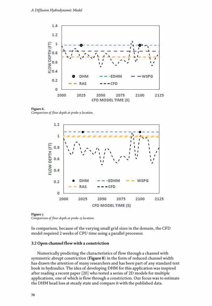
A Diffusion Hydrodynamic Model
70
In comparison, because of the varying small grid sizes in the domain, the CFD model required 2 weeks of CPU time using a parallel processor.
3.2 Open channel flow with a constriction
Numerically predicting the characteristics of flow through a channel with symmetric abrupt constriction (Figure 8) in the form of reduced channel width has drawn the attention of many researchers and has been part of any standard text book in hydraulics. The idea of developing DHM for this application was inspired after reading a recent paper [20] who tested a series of 2D models for multiple applications, one of which is flow through a constriction. Our focus was to estimate the DHM head loss at steady state and compare it with the published data.
Figure 6. Comparison of flow depth at probe 9 location.
Figure 7. Comparison of flow depth at probe 13 location.
71
Comparison of DHM Results for One- and Two-Dimensional Flows with Experimental…DOI: http://dx.doi.org/10.5772/intechopen.93212
3.2.1 Examined numerical models
The results of the extended DHM (EDHM), Mike 21, TUFLOW, and HEC-RAS 2D models were compared, with the bench mark data from the equations provided by the Federal Highways Administration (FHA). Mike 21 and HEC-RAS 2D are briefly outlined here. Mike 21 solves the two-dimensional free surface flows where stratification can be neglected. It was originally developed for flow simulation in coastal areas, estuaries, and seas. The various modules of the system simulate hydrodynamics, advection-dispersion, short waves, sediment transport, water quality, eutrophication, and heavy metals [21].
HEC-RAS 2D (5.0.1) solves the two-dimensional Saint-Venant Equations [7] for shallow water flows using the full momentum computational method. The equa-tions can model turbulence and Coriolis effects. For flow in sudden contraction, which is accompanied by high velocity, using the full momentum method in RAS 2D is recommended. The model uses an implicit finite volume solver.
3.2.2 Model variables
Figure 8 is the definition sketch of the test problem. The rectangular channel is 3100 ft long and 320 ft wide. The constriction is 60 × 60 ft. The channel length before constriction is 310 ft, and its length after constriction is 2730 ft. The compu-tational domain in EDHM had 10 ft square cells, and the total number of cells was 9920. The longitudinal slope is 1%, the transverse slope is zero, and the model was run for a total of 1 hour. The upstream inflow is 1000 cfs. Since there are 30 cells at the upstream end, a uniform steady inflow of 33.3 cfs was specified at each of the cells. At the downstream end, a free overall boundary was specified. Constricting the flow area results in loss of energy. This loss of energy is reflected in a rise in energy gradient line and energy upstream of the constriction. Of interest is to estimate the head loss that occurs between points 1 and 2 (shown in Figure 8). The head loss (HL) equals WSE2 − WSE1, where WSE is the water surface elevation [20].
3.2.3 Results
Table 1 shows the comparison of the head loss value obtained from the models along with the published data of other models. It is noted that in this effort, the computational models are compared with respect to head loss (as given in [20]) through the constriction, and this is the primary form of assessment. The DHM
Figure 8. Definition sketch of the test problem along with the location of the two points (P1 and P2).

A Diffusion Hydrodynamic Model
72
Author details
Theodore V. Hromadka II 1* and Prasada Rao2
1 Department of Mathematical Sciences, United States Military Academy, West Point, NY, USA
2 Department of Civil and Environmental Engineering, California State University, Fullerton, CA, USA
*Address all correspondence to: [email protected]
WSE change value is within the range of other model predictions, although all the model predictions are above the FHA value.
4. Conclusions
Results from multiple computer models are compared with those of DHM for one- and two-dimensional flows. The considered one-dimensional flow was a mixed flow with a hydraulic jump. All the model results (DHM, WSPG, RAS, TUFLOW) were compared with the benchmark experimental data. Because of the way the boundary conditions are specified in the DHM, the model cannot simulate the hydraulic jump. For the two-dimensional overland flow, the model results (DHM, EDHM, TUFLOW, MIKE 21, WSPG, RAS, RAS2D, and the CFD model, OpenFOAM) were compared between themselves. The agreement of the predicted flow variables reinforces the reliability of the current model.
WSE change (ft)
HEC-RAS 2D 1.27
TUFLOW 0.99
Mike 21 1.28
EDHM 1.16
FHA equation 0.8*Except for EDHM all other data were obtained from the literature [20].
Table 1. Comparison of change in water surface elevation at constriction between EDHM and published data*.
© 2020 The Author(s). Licensee IntechOpen. Distributed under the terms of the Creative Commons Attribution - NonCommercial 4.0 License (https://creativecommons.org/licenses/by-nc/4.0/), which permits use, distribution and reproduction for non-commercial purposes, provided the original is properly cited.
73
Comparison of DHM Results for One- and Two-Dimensional Flows with Experimental…DOI: http://dx.doi.org/10.5772/intechopen.93212
[1] Viti N, Valero D, Gualtieri C. Numerical simulation of hydraulic jumps. Part 2: Recent results and future outlook. Water. 2018;11:28. DOI: 10.3390/w11010028
[2] Bayón Barrachina A, López Jiménez PA. Numerical analysis of hydraulic jumps using OpenFOAM. Journal of Hydroinformatics. 2015;17(4):662-678. DOI: 10.2166/hydro.2015.041
[3] Mortazavi M, Le Chenadec V, Moin P, Mani A. Direct numerical simulation of a turbulent hydraulic jump: Turbulence statistics and air entrainment. Journal of Fluid Mechanics. 2016;797:60-94
[4] Gharangik AM, Chaudhry MH. Numerical simulation of hydraulic jump. Journal of Hydraulic Engineering ASCE. 1991;117:1195
[5] Rao P, Hromadka TV II. Numerical modeling of rapidly varying flows using HEC-RAS and WSPG models. Technical Note. Springerplus. 2016;5:662. DOI: 10.1186/s40064-016-2199-0
[6] Hirsh C. Numerical Computation of Internal and External Flows. New York (NY): John Wiley & Sons; 1990
[7] U.S. Army Corps of Engineers (USACE). HEC-RAS River Analysis System. User’s Manual. Davis, CA: Hydrologic Engineering Center; 2019. Version 5.0.7. Available from: http://www.hec.usace.army.mil/software/hec-ras/
[8] Water Surface Pressure Gradient for Windows. Joseph E. Bonadiman & Associates, Inc.; Available from: https://civildesign.com/products/wspgw-water-surface-pressure-gradient-for-windows
[9] BMT-WBM, Australia. User’s Manual for TUFLOW. Spring Hill: WBM Oceanics Australia; 2019
[10] Costabile P, Costanzo C, Macchione F, Mercogliano P. Two-dimensional model for overland flow simulations: A case study. European Water. 2012;38:13-23
[11] Ponce VM. Modeling surface runoff with kinematic, diffusion, and dynamic waves. In: Singh VP, Kumar B, editors. Proceedings of the International Conference on Hydrology and Water Resources. New Delhi, India, December 1993. Dordrecht: Water Science and Technology Library, Springer; 1996. p. 16
[12] Kazezyılmaz-Alhan CM. An improved solution for diffusion waves to overland flow. Applied Mathematical Modelling. 2012;36:465-1472
[13] Santillana M. Analysis and numerical simulation of the diffusive wave approximation of the shallow water equations [PhD thesis]. Austin: University of Texas; 2008
[14] Liu Q , Chen L, Li J, Singh V. Two-dimensional kinematic wave model of overland-flow. Journal of Hydrology. 2004;291(10):28-41
[15] Tsai T, Yang J. Kinematic wave modelling of overland flow using characteristic method with cubic-spline interpolation. Advances in Water Resources. 2005;28(7):661-670
[16] The Free Software Foundation Inc. OpenFOAM: The Open Source CFD Toolbox User Guide. London, United Kingdom: The Free Software Foundation Inc; 2019. Available from: https://openfoam.org/
[17] Weller H, Tabor G, Jasak H, Fureby C. A tensorial approach to computational continuum mechanics using object-oriented techniques. Computers in Physics. 1998;12:620-631
References

A Diffusion Hydrodynamic Model
74
[18] McDonald PW. The computation of transonic flow through two-dimensional gas turbine cascades. American Society of Mechanical Engineers. Paper No: 71-GT-89, V001T01A089; 1971. p. 7. DOI: 10.1115/71-GT-89
[19] Bayon A, Valero D, García-Bartual R, Jos F, Valles-Mor FJ, Lopez-Jim P. Performance assessment of OpenFOAM and FLOW-3D in the numerical modeling of a low Reynolds number hydraulic jump. Environmental Modelling & Software. 2016;80:322-335
[20] Paudel M, Roman SB, Pritchard J. A Comparative Study of HEC-RAS 2D, TUFLOW, & Mike 21. In: ASFPM 2016 Annual National Conference, Grand Rapids, MI. 2016
[21] DHI, MIKE 11 & MIKE 21 Flow Model. Scientific Documentations. 2019. Available from: https://www.mikepoweredbydhi.com

A Diffusion Hydrodynamic ModelAuthored by Theodore V. Hromadka II,
Chung-Cheng Yen and Prasada Rao
Authored by Theodore V. Hromadka II, Chung-Cheng Yen and Prasada Rao
The Diffusion Hydrodynamic Model (DHM), as presented in the 1987 USGS publication, was one of the first computational fluid dynamics computational
programs based on the groundwater program MODFLOW, which evolved into the control volume modeling approach. Over the following decades, others developed similar computational programs that either used the methodology and approaches
presented in the DHM directly or were its extensions that included additional components and capacities. Our goal is to demonstrate that the DHM, which was developed in an age preceding computer graphics/visualization tools, is as robust as any of the popular models that are currently used. We thank the USGS for their
approval and permission to use the content from the earlier USGS report.
Published in London, UK
© 2020 IntechOpen © PashaIgnatov / iStock
ISBN 978-1-83962-817-7
A D
iffusion H
ydrodynamic M
odel
ISBN 978-1-83962-819-1