a distributed-memory randomized structured multifrontal ...xiaj/work/mfpar.pdf · a...

SIAM J. SCI. COMPUT. c© 2017 Society for Industrial and Applied MathematicsVol. 39, No. 4, pp. C292–C318

A DISTRIBUTED-MEMORY RANDOMIZED STRUCTUREDMULTIFRONTAL METHOD FOR SPARSE DIRECT SOLUTIONS∗

ZIXING XIN† , JIANLIN XIA‡ , MAARTEN V. DE HOOP§ , STEPHEN CAULEY¶, AND

VENKATARAMANAN BALAKRISHNAN‖

Abstract. We design a distributed-memory randomized structured multifrontal solver for largesparse matrices. Two layers of hierarchical tree parallelism are used. A sequence of innovative parallelmethods are developed for randomized structured frontal matrix operations, structured update ma-trix computation, skinny extend-add operation, selected entry extraction from structured matrices,etc. Several strategies are proposed to reuse computations and reduce communications. Unlike anearlier parallel structured multifrontal method that still involves large dense intermediate matrices,our parallel solver performs the major operations in terms of skinny matrices and fully structuredforms. It thus significantly enhances the efficiency and scalability. Systematic communication costanalysis shows that the numbers of words are reduced by factors of about O(

√n/r) in two dimen-

sions and about O(n2/3/r) in three dimensions, where n is the matrix size and r is an off-diagonalnumerical rank bound of the intermediate frontal matrices. The efficiency and parallel performanceare demonstrated with the solution of some large discretized PDEs in two and three dimensions.Nice scalability and significant savings in the cost and memory can be observed from the weak andstrong scaling tests, especially for some 3D problems discretized on unstructured meshes.

Key words. distributed memory, tree parallelism, fast direct solver, randomized multifrontalmethod, rank structure, skinny matrices

AMS subject classifications. 15A23, 65F05, 65F30, 65Y05, 65Y20

DOI. 10.1137/16M1079221

1. Introduction. The solution of large sparse linear systems plays a criticallyimportant role in modern numerical computations and simulations. Generally, thereare two types of sparse solvers, iterative ones and direct ones. Direct solvers are robustand suitable for solving linear systems with multiple right-hand sides but usually takemore memory to store the factors that are often much denser. The focus of this workis on a parallel sparse direct solution that uses low-rank approximations to reducefloating-point operations and decrease memory usage.

An important type of direct solvers is the multifrontal method proposed in [9].Multifrontal methods perform the factorization of a sparse matrix via a sequenceof smaller dense factorizations organized following a tree called an elimination orassembly tree. This results in nice data locality and great potential for parallelization.Matrix reordering techniques such as nested dissection [10] are commonly used beforethe factorization to reduce fill-in.

∗Submitted to the journal’s Software and High-Performance Computing section June 9, 2016;accepted for publication (in revised form) March 13, 2017; published electronically August 17, 2017.

http://www.siam.org/journals/sisc/39-4/M107922.htmlFunding: The work of the second author was supported in part by NSF CAREER Award

DMS-1255416.†Department of Mathematics, Purdue University, West Lafayette, IN 47907 ([email protected]).‡Department of Mathematics and Department of Computer Science, Purdue University, West

Lafayette, IN 47907 ([email protected]).§Department of Computational and Applied Mathematics, Rice University, Houston, TX 77005

([email protected]).¶Athinoula A. Martinos Center for Biomedical Imaging, Department of Radiology, Massachusetts

General Hospital, Harvard University, Charlestown, MA 02129 ([email protected]).‖School of Electrical and Computer Engineering, Purdue University, West Lafayette, IN 47907

([email protected]).

C292

http://www.siam.org/journals/sisc/39-4/M107922.html

mailto:[email protected]





DISTRIBUTED-MEMORY RANDOMIZED MULTIFRONTAL SOLVER C293

In recent years, structured multifrontal methods [33, 30, 27, 2] have been devel-oped to utilize a certain low-rank property of the intermediate dense matrices thatarise in the factorization of some discretized PDEs. This low-rank property has beenfound in many problems, such as the ones arising from the discretization of ellipticPDEs. Hierarchical structured matrices like H/H2-matrices [5, 15, 17] and hierar-chically semiseparable (HSS) matrices [6, 34] are often used to take advantage of thelow-rank property. Other rank structured representations are also used in multifrontaland similar solvers [2, 14].

To enhance the performance and flexibility of the structured matrix operations,some recent work integrates randomization into structured multifrontal methods [31].Randomized sampling enables the conversion of a large rank-revealing problem intoa much smaller one after matrix-vector multiplications [18, 21]. This often greatlyaccelerates the construction of structured forms and also makes the processing of thedata much simpler [24, 35].

In this work, we are interested in the parallelization of the randomized struc-tured multifrontal (RSMF) method in [31] for the factorization of large-scale sparsematrices. The work is a systematic presentation of our developments in the technicalreports [36, 37, 38]. The parallelism is essential to speed up the algorithms and makethe algorithms available to large problems by the exploitation of more processes andmemory. Earlier work in [28] gives a parallel multifrontal solver based on a simpli-fied structured multifrontal method in [30] that involves dense intermediate matrices.Some dense matrices called frontal matrices are approximated by HSS forms and thenfactorized. The resulting Schur complements called update matrices are still denseand are used to assemble later frontal matrices. The use of dense update matricesis due to the lack of an effective structured data assembly strategy. All these densematrices tend to be a memory bottleneck if their sizes are large. Moreover, the denseforms make some major operations more costly than necessary, including the struc-tured approximations of the frontal matrices, the computation of the update matrices,and the assembly of the frontal matrices. In addition, the parallel solver in [28] relieson the geometry of the mesh, which is required to be a regular mesh. This limits theapplicability of that solver.

Here, we seek to build a systematic framework for parallelizing the RSMF methodin [31] using distributed memory. The randomized approach avoids the use of densefrontal and update matrices and also makes the parallelization significantly moreconvenient and efficient. We also allow more general matrix types. Our main resultsinclude the following:

• We design all the mechanisms for a distributed-memory parallel implemen-tation of the RSMF method. A static mapping parallel model is designedto handle two layers of parallelism (one for the assembly tree and anotherfor the structured frontal/update matrices) as well as new parallel structuredoperations. Novel parallel algorithms for all the major steps are developed,such as the intermediate structured matrix operations, structured submatrixextraction, skinny matrix assembly, and information propagation.

• A sequence of strategies is given to reduce the communication costs, suchas the combination of process grids for different tree parallelism, a compactstorage of HSS forms, the assembly and passing of data between processesin compact forms, heavy data reuse, the collection of data for BLAS3 op-erations, and the storage of a small amount of the same data in multipleprocesses.

C294 XIN, XIA, DE HOOP, CAULEY, AND BALAKRISHNAN

• The parallel structured multifrontal method is not restricted to a specific meshgeometry. Graph partitioning techniques and packages are used to efficientlyproduce nested dissection ordering of a general mesh. The method can beapplied to much more general sparse matrices where the low-rank propertyexists. For problems without the low-rank property, we can also use themethod as an effective preconditioner.

• Our nested dissection ordering and symbolic factorization well respect thelocal geometric connectivity and thus naturally preserve the inherent low-rank property in the intermediate dense matrices.

• As compared with the parallel structured multifrontal method in [28],– our parallel method can be applied to sparse matrices corresponding to

more general graphs instead of only regular meshes;– we do not need to store large dense frontal/update matrices or convert

between dense and HSS matrices, and instead, the HSS constructionsand factorizations are fully structured;

– the parallel data assembly is performed through skinny matrix-vectorproducts instead of large dense matrices.

We give a detailed analysis of the communication cost (which is also missingfor the method in [28]). The communication cost of our solver includes O(

√P ) +

O(r log3 P ) messages and O( r√n

P)+O( r

2 log3 P√P

) words for two-dimensional (2D) prob-

lems or O( rn23

P) + O( r

2 log3 P√P

) words for 3D problems, where n is the matrix size, P

is the total number of processes, r is the maximum off-diagonal numerical rank ofthe frontal matrices, and P is the minimum size of all the process grids. There is asignificant reduction in the communication cost as compared with the solver in [28].The numbers of words of the new solver are smaller by factors about O(

√nr ) and

O(n23

r ) for two and three dimensions, respectively.Extensive numerical tests in terms of some discretized PDEs in two and three

dimensions are used to show the parallel performance. Both weak and strong scalingtests are done. The nice scalability and significant savings in the cost and memorycan be clearly observed, especially for some 3D PDEs discretized on unstructuredmeshes. For example, for a discretized 3D Helmholtz equation with n ≈ 9.7×106, thenew solver takes about 1/4 of the flops of the standard multifrontal solver and about1/2 of the storage for the factors. With up to 256 processes, when the number ofprocesses doubles, the parallel factorization time reduces by a factor about 1.7 ∼ 1.8.The new solver works well for larger n even if the standard parallel multifrontal solverruns out of memory.

The remaining sections are organized as follows. We discuss nested dissection,parallel symbolic factorization, and graph connectivity preservation in section 2. Sec-tion 3 reviews the basic framework of the RSMF method. Section 4 details our parallelrandomized structured multifrontal (PRSMF) method. Section 5 shows the analysisof the communication cost. The numerical results are shown in section 6. Finally, wedraw our conclusions in section 7.

For convenience, we first explain the basic notation to be used throughout thepaper.

• For a matrix A and an index set I, A|I denotes the submatrix of A formedby the rows with the row index set I.

• For a matrix A and index sets I,J, A|I×J denotes the submatrix of A withrow index set I and column index set J.


• If T is a postordered binary tree with nodes i = 1, 2, . . ., we use sib(i) andpar(i) to denote the sibling and parent of a node i, respectively, and useroot(T ) to denote the root node of T .

• Bold and calligraphic letters are usually used for symbols related to the mul-tifrontal process.

2. Nested dissection for general graphs, parallel symbolic factorization,and connectivity preservation. For an n × n sparse matrix A, let G(A) be itscorresponding adjacency graph, which has n vertices and has an edge connectingvertices i and j if Aij 6= 0. G is a directed graph if A is nonsymmetric. In this case,we consider the adjacency graph G(A+AT ) instead of G(A) (see, e.g., [3, 20]). In thefactorization of A, vertices in the adjacency graph are eliminated, and their neighborsare connected, which yields fill-in in the factors.

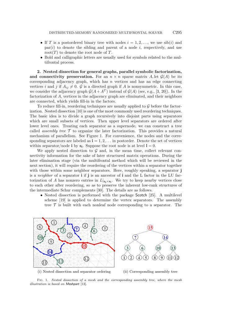
To reduce fill-in, reordering techniques are usually applied to G before the factor-ization. Nested dissection [10] is one of the most commonly used reordering techniques.The basic idea is to divide a graph recursively into disjoint parts using separatorswhich are small subsets of vertices. Then upper level separators are ordered afterlower level ones. Treating each separator as a supernode, we can construct a treecalled assembly tree T to organize the later factorization. This provides a naturalmechanism of parallelism. See Figure 1. For convenience, the nodes and the corre-sponding separators are labeled as i = 1, 2, . . . in postorder. Denote the set of verticeswithin separator/node i by si. Suppose the root node is at level l = 0.

We apply nested dissection to G and, in the mean time, collect relevant con-nectivity information for the sake of later structured matrix operations. During thelater elimination stage (via the multifrontal method which will be reviewed in thenext section), it will require the reordering of the vertices within a separator togetherwith those within some neighbor separators. Here, roughly speaking, a separator jis a neighbor of a separator i if j is an ancestor of i and the L factor in the LU fac-torization of A has nonzero entries in L|sj×si . We try to keep nearby vertices closeto each other after reordering, so as to preserve the inherent low-rank structures ofthe intermediate Schur complements [30]. The details are as follows.

• Nested dissection is performed with the package Scotch [25]. A multilevelscheme [19] is applied to determine the vertex separators. The assemblytree T is built with each nonleaf node corresponding to a separator. The

8

9

12

14

5

11

2

3

10

13

6

14

7

15

15

4

3 6 1

7 1

0 13

1 2 4 5 8 9 11 12

(i) Nested dissection and separator ordering (ii) Corresponding assembly tree

Fig. 1. Nested dissection of a mesh and the corresponding assembly tree, where the meshillustration is based on Meshpart [13].


Gibbs–Poole–Stockmeyer method [12] is used to order the vertices within eachseparator so that the bandwidth of the corresponding adjacency submatrix ofA is small. Geometrically, this keeps nearby vertices within a separator closeto each other under the new ordering and may benefit the low-rank structureof the corresponding frontal matrix. The reason is as follows. For somediscretized elliptic PDEs, the frontal matrices are related to (the inverses of)the discretized Green’s functions, and the low-rank property of the frontalmatrices is related to the geometric separability of the mesh points wherethe Green’s function is evaluated [7, 33]. Well-separated points correspondto blocks with small numerical ranks. Thus intuitively, it is often beneficialto use an appropriate ordering that respects the geometric connectivity.

• In a symbolic factorization, following a bottom-up traversal of the assemblytree T , we collect the neighbor information of each node of T . The neighborinformation reflects how earlier eliminations create fill-in. The connectivityof the vertices within a separator i and its neighbors is also collected. Suchconnectivity information is accumulated from child nodes to parent nodes andis used to preserve the graph connectivity after reordering.

• The symbolic factorization is performed in parallel. Under a certain paral-lel level lp, each process performs a local symbolic factorization of a privatesubtree and stores the corresponding neighboring information. At level lp, anall-to-all communication between all processes is triggered to exchange neigh-boring information of nodes at lp. For all the nodes above lp, the symbolicfactorization is performed within each processor, so that each process canconveniently access relevant nodes without extra communications.

• Following the nice data locality of the assembly tree, we adopt a subtree-to-subcube static mapping model [11] to preallocate computational tasks toeach process. Each process is assigned a portion of the computational tasksassociated with a subtree of T or a subgraph of G. Starting from a certainlevel, processes form disjoint process groups form process grids to work to-gether. We try to evenly divide the adjacency graph so as to maintain theload balance of processes. See also section 4.1. Static unbalances may stillexist as a result of unbalanced partitioning of the graph. Dynamic unbal-ances may also arise in the factorization stage since the HSS ranks and HSSgenerator sizes are generally unknown in advance. It will be interesting to in-vestigate the use of dynamic scheduling in our solver. Other static mappingmodels such as the strict proportional mapping [26] are also used in somesparse direct solvers and may help improve the static balance of our solver.These are not the primary focus of the current work and will be studied in thefuture.

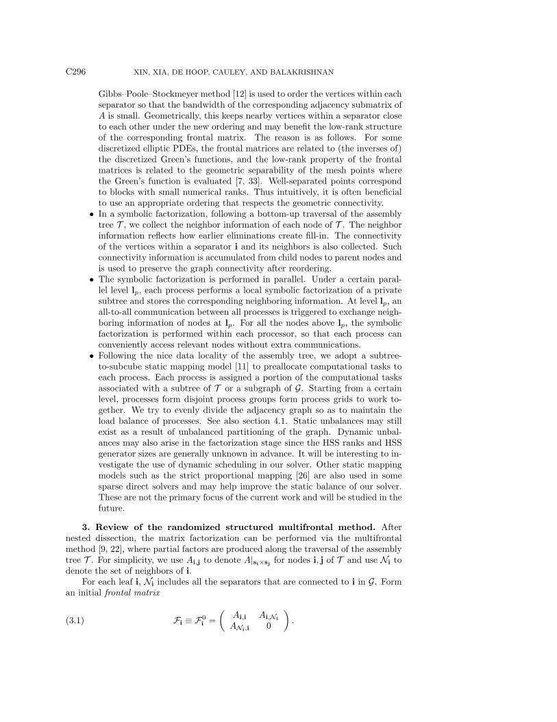
3. Review of the randomized structured multifrontal method. Afternested dissection, the matrix factorization can be performed via the multifrontalmethod [9, 22], where partial factors are produced along the traversal of the assemblytree T . For simplicity, we use Ai,j to denote A|si×sj for nodes i, j of T and use Ni todenote the set of neighbors of i.

For each leaf i, Ni includes all the separators that are connected to i in G. Forman initial frontal matrix

(3.1) Fi ≡ F0i =

(Ai,i Ai,Ni

ANi,i 0

).


Compute an LU factorization of Fi:

(3.2) Fi =(

Li,i

LNi,i I

)(Ki,i Ki,Ni

Ui

),

where Ui is the Schur complement and is called an update matrix. In the adjacencygraph, this corresponds to the elimination of i.

For each nonleaf node i, Ni includes all the ancestor separators that are originallyconnected to i in G or get connected due to lower level eliminations. Suppose thechild nodes of i are c1 and c2. Form a frontal matrix

(3.3) Fi = F0i↔l Uc1↔l Uc2 ,

where the symbol↔l denotes the extend-add operation [9, 22]. This operation performsmatrix permutation and addition by matching the index sets following the orderingof the vertices in G. Then partition Fi as

(3.4) Fi =(Fi;1,1 Fi;1,2Fi;2,1 Fi;2,2

),

where Fi;1,1 corresponds to si, and perform an LU factorization as in (3.2).The above procedure continues along the assembly tree until the root is reached.

This is known as the standard multifrontal method. A bottleneck of the method isthe storage and cost associated with the local dense frontal and update matrices.

The class of structured multifrontal methods [30, 31, 33] is based on the ideathat, for certain matrices A, the local dense frontal and update matrices are rankstructured. For some cases, Fi and Ui may be approximated by rank structuredforms such as HSS forms. An HSS matrix F is a hierarchical structured form thatcan be defined via a postordered binary tree T called an HSS tree. Each node i of Tis associated with some local matrices called generators that are used to define F . Adiagonal generator Di is recursively defined, so that Dk ≡ F for the root k of T , andfor a node i with children c1 and c2,

Di =(

Dc1 Uc1Bc1VTc2

Uc2Bc2VTc1 Dc2

),

where the off-diagonal basis generators U, V are also recursively defined as

Ui =(Uc1Rc1Uc2Rc2

), Vi =

(Vc1Wc1

Vc2Wc2

).

Suppose Di corresponds to an index set si ⊂ 1 : N, where N is the size of F ; thenF−i ≡ F |si×(1:N\si) and F |i ≡ F |(1:N\si)×si

are called HSS blocks, whose maximum(numerical) rank is called the HSS rank of F . Also for convenience, suppose the rootnode of T is at level l = 0.

In the structured multifrontal method in [33], HSS approximations to the frontalmatrices are constructed. The factorization of an HSS frontal matrix Fi yields an HSSupdate matrix Ui. This process may be costly and complex. A simplified version in[28] uses dense Ui instead. To enhance the efficiency and flexibility, randomized HSSconstruction [24, 35] is used in [31]. The basic idea is to compress the off-diagonalblocks of Fi via randomized sampling [21]. Suppose Fi has size N × N and HSS


rank r. Generate an N × (r + µ) Gaussian random matrix X, where µ is a smallinteger. Compute

(3.5) Y = FiX.

The compression of an HSS block F−i ≡ Fi|si×(1:N\si) is done via the compressionof

(3.6) Si = Y −DiX|si(= F−i X|1:N\si

).

Applying a strong rank-revealing factorization [16] to the above quantity yields

Si ≈ UiSi|siwith Ui = Πi

(IEi

),

where si is a subset of si and the entries of Ei have magnitudes around 1. This givesthe U generator in the HSS construction, so that F−i ≈ UiF

−i |si

with high probability[21]. Due to the feature that the row basis matrix F−i |si

is a submatrix of F−i , thiscompression is also referred to as a structure-preserving rank-revealing factorization[35]. More details for generating the other HSS generators can be found in [24, 35].The overall HSS construction follows a bottom-up sweep of the HSS tree.

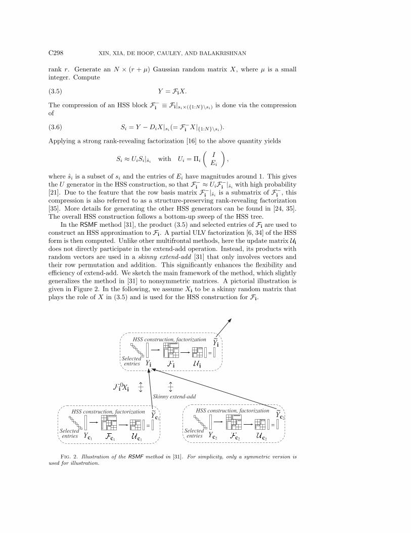
In the RSMF method [31], the product (3.5) and selected entries of Fi are used toconstruct an HSS approximation to Fi. A partial ULV factorization [6, 34] of the HSSform is then computed. Unlike other multifrontal methods, here the update matrix Uidoes not directly participate in the extend-add operation. Instead, its products withrandom vectors are used in a skinny extend-add [31] that only involves vectors andtheir row permutation and addition. This significantly enhances the flexibility andefficiency of extend-add. We sketch the main framework of the method, which slightlygeneralizes the method in [31] to nonsymmetric matrices. A pictorial illustration isgiven in Figure 2. In the following, we assume Xi to be a skinny random matrix thatplays the role of X in (3.5) and is used for the HSS construction for Fi.

=

Yc1

Yc1 c1 c1

Xii0

Skinny extend-add

=

Yc2

Yc2 c2 c2

=

Yi

Selectedentries Yi i i

HSS construction, factorization

HSS construction, factorization HSS construction, factorization

Selectedentries

Selectedentries

~ ~

~

Fig. 2. Illustration of the RSMF method in [31]. For simplicity, only a symmetric version isused for illustration.


1. For nodes i below a certain switching level ls of T , perform the traditionalmultifrontal factorization.

2. For nodes i above level ls, construct an HSS approximation to Fi using se-lected entries of Fi and matrix-vector products Yi = FiXi and Zi = FTi Xi.Here, Yi and Zi are obtained from (3.8) below.

3. Partially ULV factorize Fi and compute Ui with the fast Schur complementupdate in HSS form. Compute

(3.7) Yi = UiXi, Zi = UTi Xi,

where Xi is a submatrix of Xi corresponding to the indices Ui as in (3.2).4. For an upper level node i with children c1 and c2, compute skinny extend-add

operations

(3.8) Yi = (F0i Xi) −l Yc1 −l Yc2 , Zi = ((F0

i )TXi) −l Zc1 −l Zc2 .

5. Form selected entries of Fi based on F0i , Uc1 , and Uc2 , and go to step 2.

4. Distributed-memory parallel randomized multifrontal method. Here,we present our distributed-memory parallel sparse direct solver based on the RSMFmethod, denoted PRSMF. The primary significance includes the following:

• We design a static mapping parallel model that (1) has two hierarchical layersof parallelism with good load balance and (2) can conveniently handle bothHSS matrices and intermediate skinny matrices. The PRSMF method signif-icantly extends the one in [28] by allowing more flexible parallel structuredoperations and also avoiding large dense intermediate frontal and update ma-trices.

• We develop some innovative parallel algorithms for a sequence of HSS opera-tions, such as a parallel HSS Schur complement computation in partial ULVfactorization, a parallel extraction of selected entries from an HSS form, anda parallel skinny extend-add algorithm for assembling local data.

• The main ideas to reduce the communication costs in the new parallel al-gorithms are (1) taking advantage of the tree parallelism and store HSSgenerators in an appropriate way; (2) assembling and passing data betweenprocesses in compact forms so that the number of messages is reduced; (3)reusing data whenever possible; (4) collecting data into messages to facilitateBLAS3 dense operations; and (5) storing a small amount of the same data inmultiple processes.

• The graph reordering strategies and the convenient data assembly make themethod much more general than the parallel structured multifrontal methodin [28] which is restricted to a specific mesh geometry.

In this section, an overview of the parallel model is given, followed by details ofthe parallel algorithms.

4.1. Overview of the parallel model and data distribution. In the RSMFmethod, both the assembly tree and the HSS tree have nice data locality. For adistributed memory architecture, a static mapping model usually requires less com-munication than a dynamic scheduling model. To avoid idling as much as possible, itis vital to keep work load balance among all processes. When generating the assemblytree and local HSS trees, we try to make the trees as balanced as possible. A roughlybalanced assembly tree can be obtained with Scotch [25] with appropriate strategies.More specifically, a multilevel graph partition method in [19] is used to generate the


3

1 2

70

6

4 5

0 1

150 1

10

8 9

141

13

11 12

Switching

30

31

Processes

Process grid

Parallellevel lp

level ls

0 1

2 3

32

2 3

32

0 1

32

18

16 17

222

21

19 20

25

23 24

293

28

26 27

0 1 2 3

0 1 320 1

0 1 2 3

32

0 132

0 1

0 1 0 1 32 32

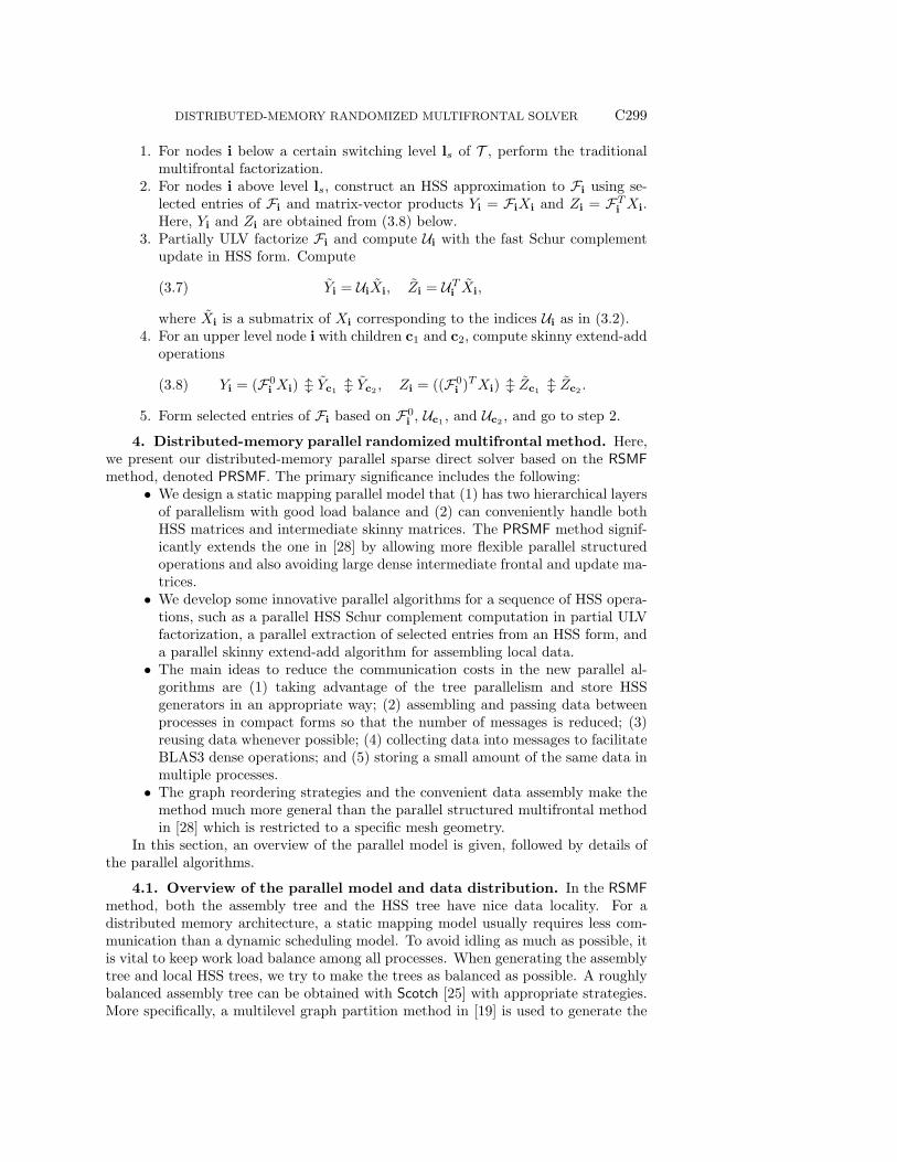
Fig. 3. Static mapping model for our PRSMF method, where the outer-layer tree is the assemblytree, and the inner-layer trees are HSS trees.

separators of the adjacency graph of A. In this method, each time we use the vertexgreedy-graph-growing method to obtain a rough separator, and refine this separatorwith some strategies so that the resulting lower level subgraphs are roughly balanced.For the HSS trees, we try to keep them balanced via the recursive bipartition of theindex set of a frontal matrix.

Our parallel model (Figure 3) is described as follows. The basic idea is inher-ited from [28], and we further incorporate more structured forms to avoid densefrontal/update matrices and also allow more flexible choices of processes for the struc-tured operations. Below a parallel level lp, one process is used to handle the operationscorresponding to one subtree, called a local tree. (The method also involves a switch-ing level ls, at which the local operations switch from dense to HSS ones so as tooptimize the complexity and also to avoid structured operations for very small ma-trices at lower levels [31].) Starting from level lp, processes are grouped into processgrids or contexts to work on larger matrices. The standard 2D block cyclic storagescheme in ScaLAPACK [4] is adopted to store dense blocks (such as HSS generatorsand skinny matrices). Process grids associated with the nodes of the assembly treeT are generated as follows. Let Gi denote the set of processes assigned to a node i.Then,

• Gi ∩Gj = ∅ if i and j are distinct nodes at the same level;• Gi = Gc1 ∪ Gc2 for a parent node i with child nodes c1 and c2. Usually,

the process grids associated with Gc1 and Gc2 are concatenated vertically orhorizontally to form the process grid associated with Gi. With this approach,only pairwise exchanges between the processes are needed when redistributingmatrices from the children process grids to the parent process grids. This canhelp reduce the number of messages exchanged and save the communicationcost. See [28, 29] for more discussions. Here, since the algorithm frequentlyinvolves skinny matrices, the process grids are not necessarily square. This isdifferent from those in [28, 29], where large local matrices are involved.

In this setting, each process can only access a subset of nodes in the assemblytree. We call these nodes accessible nodes of a process. The accessible nodes of aprocess are those in the associated local tree and in the path connecting the rootof the local tree and the root of the assembly tree. For example, in Figure 3, the


accessible nodes of process 0 are nodes 1, 2, . . . , 7, 15, 31. A process only gets involvedin the computations associated with its accessible nodes.

Along the assembly tree, child nodes pass information to parent nodes, and com-munication between two process groups is involved. Unlike the traditional multifrontalmethod and the structured one in [28] that pass dense update matrices, here, onlyskinny matrix-vector products and a small number of matrix entries are passed. Onthe process grid of a parent node, we redistribute these skinny matrices to the corre-sponding processes. We design a distribution scheme and a message passing methodto perform the skinny extend-add operation in parallel. The result will be used in theparallel randomized HSS construction.

For a node i above lp, if HSS operations are involved, smaller process subgroupsare formed by the processes in Gi to accommodate the parallel HSS operations forFi, Ui, etc. For each node i of the HSS tree T of Fi, a process group Gi ⊂ Gi isformed. Initially, for the root k of T , Gk ≡ Gi, which is used for both Fi and Ui.Unlike the scheme in [23], Gk is also used for both children of k, so as to facilitatethe computation of Ui. (See the inner-layer trees in Figure 3.) For nodes at lowerlevels, the same strategies to group processes as above are used along the HSS treeto form the process subgroups. That is, for any nonleaf node i of T below level 1,Gi = Gc1 ∪Gc2 , where children c1 and c2 are the children of i. Each process subgroupforms a process grid which stores the dense blocks (such as HSS generators and skinnymatrices) in a 2D block cyclic scheme. The operations (such as multiplication andredistribution) on the dense blocks are performed with ScaLAPACK. As in [23], theHSS generators Ri,Wi (and also Di, Ui for a leaf i) are stored in Gi, and Bi is storedin Gpar(i). The details of these grouping and distribution schemes will become clearin the subsequent subsections.

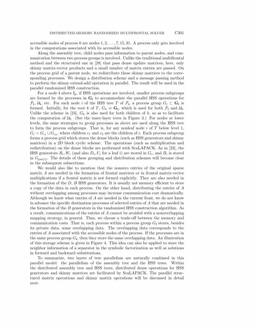
We would also like to mention that the nonzero entries of the original sparsematrix A are needed in the formation of frontal matrices or in frontal matrix-vectormultiplications if a frontal matrix is not formed explicitly. They are also needed inthe formation of the D, B HSS generators. It is usually not memory efficient to storea copy of the data in each process. On the other hand, distributing the entries of Awithout overlapping among processes may increase communication cost dramatically.Although we know what entries of A are needed in the current front, we do not knowin advance the specific destination processes of selected entries of A that are needed inthe formation of the B generators in the randomized HSS construction algorithm. Asa result, communications of the entries of A cannot be avoided with a nonoverlappingmapping strategy, in general. Thus, we choose a trade-off between the memory andcommunication costs. That is, each process within a process group Gi stores, besidesits private data, some overlapping data. The overlapping data corresponds to theentries of A associated with the accessible nodes of the process. If the processes are inthe same process group Gi, then they store the same overlapping data. An illustrationof this storage scheme is given in Figure 4. This idea can also be applied to store theneighbor information of a separator in the symbolic factorization as well as solutionsin forward and backward substitutions.

To summarize, two layers of tree parallelism are naturally combined in thisparallel model: the parallelism of the assembly tree and the HSS trees. Withinthe distributed assembly tree and HSS trees, distributed dense operations for HSSgenerators and skinny matrices are facilitated by ScaLAPACK. The parallel struc-tured matrix operations and skinny matrix operations will be discussed in detailnext.


Private data Overlapping data

Process 1

Process 2

l=l p ...

l=0

l=1

......

Process ...

l=l p ...

l=0

l=1

l=l p ...

l=0

l=1

Fig. 4. Storage scheme for the sparse matrix A. Below the parallel level lp, each process storesa private portion of A. Above lp, each process stores overlapping data associated with its accessiblenodes at each level l = 0, 1, . . . , lp.

4.2. Parallel randomized HSS construction, factorization, and Schurcomplement computation. Above the switching level ls, all frontal and updatematrices are in HSS forms. The method in [28] is only partially structured in the sensethat dense frontal matrices are formed first and then converted into HSS forms, andthe updated matrices are also dense. Here, the HSS construction for a frontal matrixFi is done via randomization, and a partial ULV factorization of Fi also produces anHSS form Schur complement/update matrix Ui in (3.2).

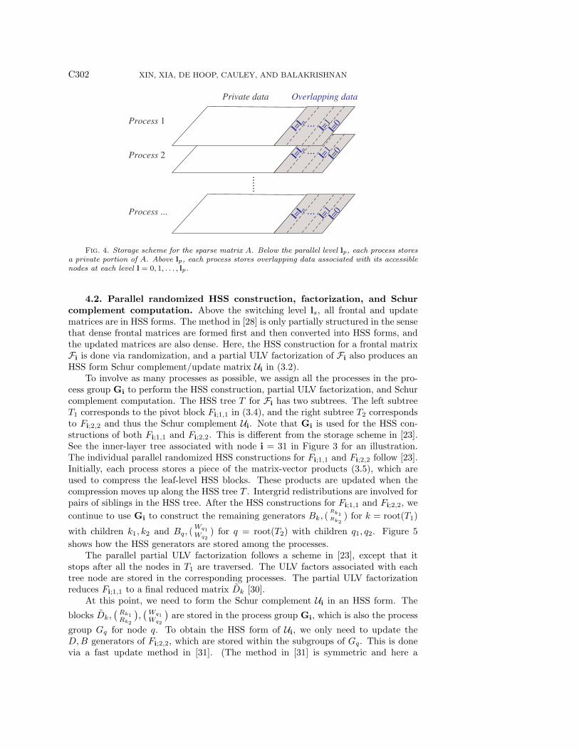
To involve as many processes as possible, we assign all the processes in the pro-cess group Gi to perform the HSS construction, partial ULV factorization, and Schurcomplement computation. The HSS tree T for Fi has two subtrees. The left subtreeT1 corresponds to the pivot block Fi;1,1 in (3.4), and the right subtree T2 correspondsto Fi;2,2 and thus the Schur complement Ui. Note that Gi is used for the HSS con-structions of both Fi;1,1 and Fi;2,2. This is different from the storage scheme in [23].See the inner-layer tree associated with node i = 31 in Figure 3 for an illustration.The individual parallel randomized HSS constructions for Fi;1,1 and Fi;2,2 follow [23].Initially, each process stores a piece of the matrix-vector products (3.5), which areused to compress the leaf-level HSS blocks. These products are updated when thecompression moves up along the HSS tree T . Intergrid redistributions are involved forpairs of siblings in the HSS tree. After the HSS constructions for Fi;1,1 and Fi;2,2, wecontinue to use Gi to construct the remaining generators Bk, (

Rk1Rk2

) for k = root(T1)

with children k1, k2 and Bq, (Wq1Wq2

) for q = root(T2) with children q1, q2. Figure 5shows how the HSS generators are stored among the processes.

The parallel partial ULV factorization follows a scheme in [23], except that itstops after all the nodes in T1 are traversed. The ULV factors associated with eachtree node are stored in the corresponding processes. The partial ULV factorizationreduces Fi;1,1 to a final reduced matrix Dk [30].

At this point, we need to form the Schur complement Ui in an HSS form. The

blocks Dk,(Rk1Rk2

),(Wq1Wq2

)are stored in the process group Gi, which is also the process

group Gq for node q. To obtain the HSS form of Ui, we only need to update theD,B generators of Fi;2,2, which are stored within the subgroups of Gq. This is donevia a fast update method in [31]. (The method in [31] is symmetric and here a


( )Rk10 12 3

0 1

Rk2

Bk (Wq1,Wq2)T T

V1T

U2

001

0 1

2 3

0 12 3

0 12 3

0 12 3

1

2

3

0

1

2

3

23

2 3

Pivot block Fi;1,1

D1

B2

0 12 3

0 1

2 3

0 101

D2

Fi;2,2

Fig. 5. Distributed memory storage for an HSS form frontal matrix Fi given four processes,where k1, k2 are the children of k (root of the HSS tree T1 for Fi;1,1) and q1, q2 are the children of q(root of the HSS tree T2 for Fi;2,2). See the inner-layer tree associated with node i=31 in Figure 3.

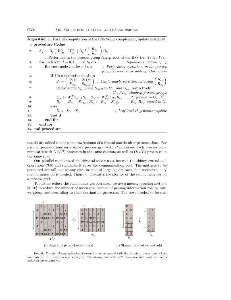
nonsymmetric variation is used.) The computations are performed in disjoint processgroups at each level in a top-down traversal of T2. A sequence of products Si arecomputed for the update. Each Si is computed in Gi and then redistributed for reuseat lower levels. Its submatrices are used to update the generators Di, Bi. The detailsare given in Algorithm 1. An important observation from this update process is thatthe HSS rank of Ui is bounded by that of Fi [30].

After this, we then compute Yi and Zi in (3.7) in parallel. This may be based ondirect HSS matrix-vector multiplications, or an indirect procedure [31] that updatesYi. The detailed parallelization is omitted here. Yi and Zi are passed to the parentnode to participate in the skinny extend-add operation.

Remark 4.1. In our solver, the nested HSS structure has a very useful feature thatsignificantly simplifies one major step: the formation of the Schur complement/updatematrix (the mathematical scheme behind Algorithm 1). That is, the nested HSSstructure enables the Schur complement computation to be conveniently done viasome reduced matrices, so that only certain generators of the frontal matrix need tobe quickly updated. Such a mathematical scheme was designed and proved in [30,31]. For 3D problems, the HSS structure is indeed less efficient than more advancedstructures such asH2 and multilayer hierarchical structures [32]. The HSS form servesas a compromise between the efficiency and the implementation simplicity.

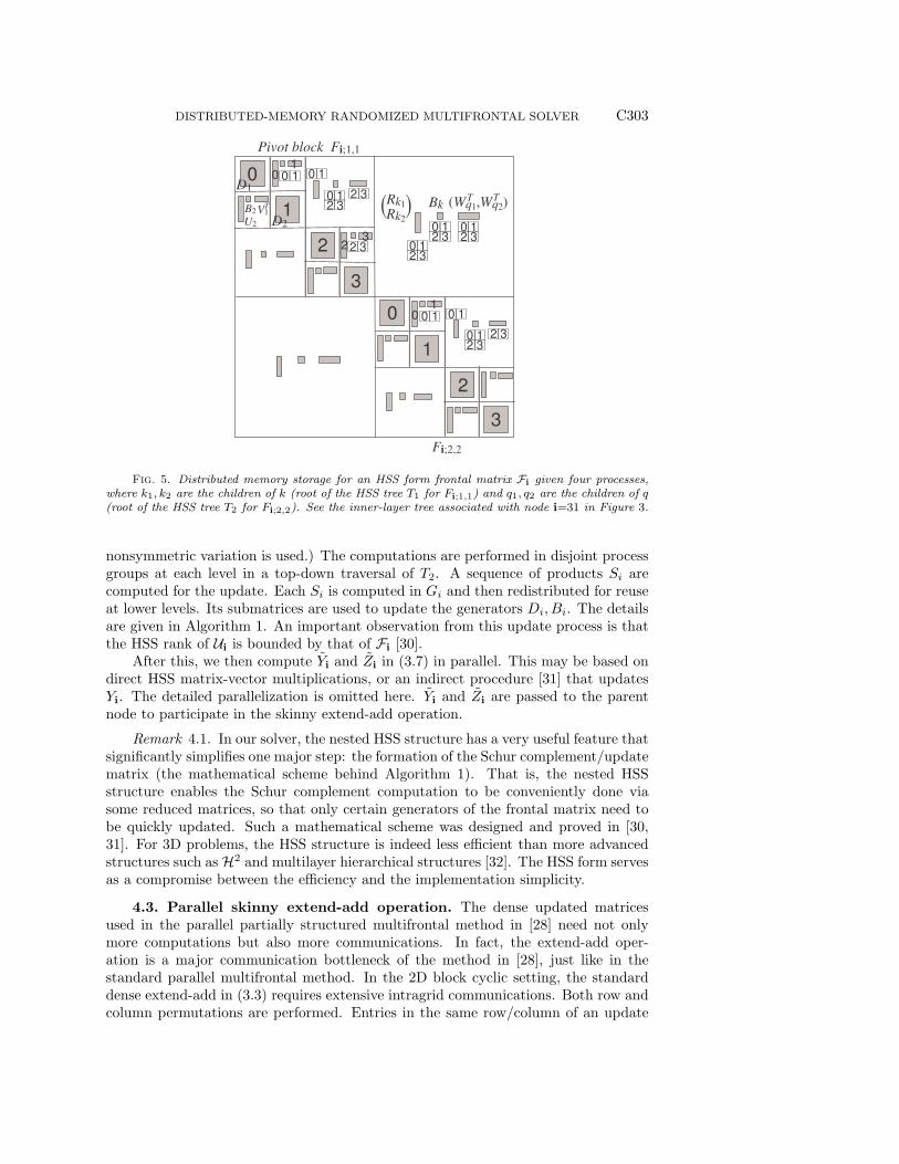
4.3. Parallel skinny extend-add operation. The dense updated matricesused in the parallel partially structured multifrontal method in [28] need not onlymore computations but also more communications. In fact, the extend-add oper-ation is a major communication bottleneck of the method in [28], just like in thestandard parallel multifrontal method. In the 2D block cyclic setting, the standarddense extend-add in (3.3) requires extensive intragrid communications. Both row andcolumn permutations are performed. Entries in the same row/column of an update


Algorithm 1. Parallel computation of the HSS Schur complement/update matrix Ui.1: procedure PSchur

2: Sq ← Bq(WTq1 WT

q2

)D−1k

(Rk1Rk2

)Bk

. Performed in the process group Gq; q: root of the HSS tree T2 for Fi;2,23: for each level l = 0, 1, . . . of T2 do . Top-down traversal of T24: for each node i at level l do . Performing operations in the process

group Gi and redistributing information5: if i is a nonleaf node then

6: Si =(Si;1,1 Si;1,2Si;2,1 Si;2,2

). Conformable partition following

(Rc1Rc2

)7: Redistribute Si;1,1 and Si;2,2 to Gc1 and Gc2 , respectively

. Gc1 , Gc2 : children process groups8: Sc1 ←WT

c1Si;1,1Rc1 , Sc2 ←WTc2Si;2,2Rc2 . Performed in Gc1 , Gc2

9: Bc1 ← Bc1 − Si;1,2, Bc2 ← Bc2 − Si;2,1 . Bc1 , Bc2 : stored in Gi10: else11: Di ← Di − Si . Leaf level D generator update12: end if13: end for14: end for15: end procedure

matrix are added to one same row/column of a frontal matrix after permutations. Forparallel permutations on a square process grid with P processes, each process com-municates with O(

√P ) processes in the same column, as well as O(

√P ) processes in

the same row.Our parallel randomized multifrontal solver uses, instead, the skinny extend-add

operations (3.8) and significantly saves the communication cost. The matrices to bepermuted are tall and skinny ones instead of large square ones, and moreover, onlyrow permutation is needed. Figure 6 illustrates the storage of the skinny matrices ona process grid.

To further reduce the communication overhead, we use a message passing method[3, 20] to reduce the number of messages. Instead of passing information row by row,we group rows according to their destination processes. The rows needed to be sent

0 1 2 3

4 5 6 7

8 9 10 11

1213 14 15

0 1 2 3

4 5 6 7

8 9 10 11

1213 14 15

0 1 2 3

4 5 6 7

8 9 10 11

1213 14 15

0 1 2 3

4 5 6 7

8 9 10 11

1213 14 15

0 1 2 3

4 5 6 7

8 9 10 11

1213 14 15

0 1

4 5

8 9

1213

0 1 2 3

4 5 6 7

0 1

4 5

c1

c2

0 1

2 3

0 1

2 3

0 1

2 3

0 1

2 3

Yc1

~

0 1

2 3

0 1

2 3

0 1

2 3

Yc2

~

(i) Standard parallel extend-add (ii) Skinny parallel extend-add

Fig. 6. Parallel skinny extend-add operation as compared with the standard dense one, wherethe matrices are stored on a process grid. The skinny one deals with much less data and also needsonly row permutations.


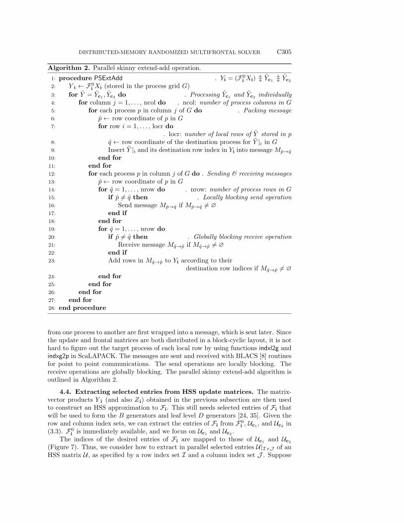
Algorithm 2. Parallel skinny extend-add operation.

1: procedure PSExtAdd . Yi = (F0i Xi) −l Yc1 −l Yc2

2: Y i ← F0i Xi (stored in the process grid G)

3: for Y = Yc1 , Yc2 do . Processing Yc1 and Yc2 individually4: for column j = 1, . . . , ncol do . ncol: number of process columns in G5: for each process p in column j of G do . Packing message6: p← row coordinate of p in G7: for row i = 1, . . . , locr do

. locr: number of local rows of Y stored in p8: q ← row coordinate of the destination process for Y |i in G9: Insert Y |i and its destination row index in Yi into message Mp→q

10: end for11: end for12: for each process p in column j of G do . Sending & receiving messages13: p← row coordinate of p in G14: for q = 1, . . . , nrow do . nrow: number of process rows in G15: if p 6= q then . Locally blocking send operation16: Send message Mp→q if Mp→q 6= ∅17: end if18: end for19: for q = 1, . . . , nrow do20: if p 6= q then . Globally blocking receive operation21: Receive message Mq→p if Mq→p 6= ∅22: end if23: Add rows in Mq→p to Yi according to their

destination row indices if Mq→p 6= ∅24: end for25: end for26: end for27: end for28: end procedure

from one process to another are first wrapped into a message, which is sent later. Sincethe update and frontal matrices are both distributed in a block-cyclic layout, it is nothard to figure out the target process of each local row by using functions indxl2g andindxg2p in ScaLAPACK. The messages are sent and received with BLACS [8] routinesfor point to point communications. The send operations are locally blocking. Thereceive operations are globally blocking. The parallel skinny extend-add algorithm isoutlined in Algorithm 2.

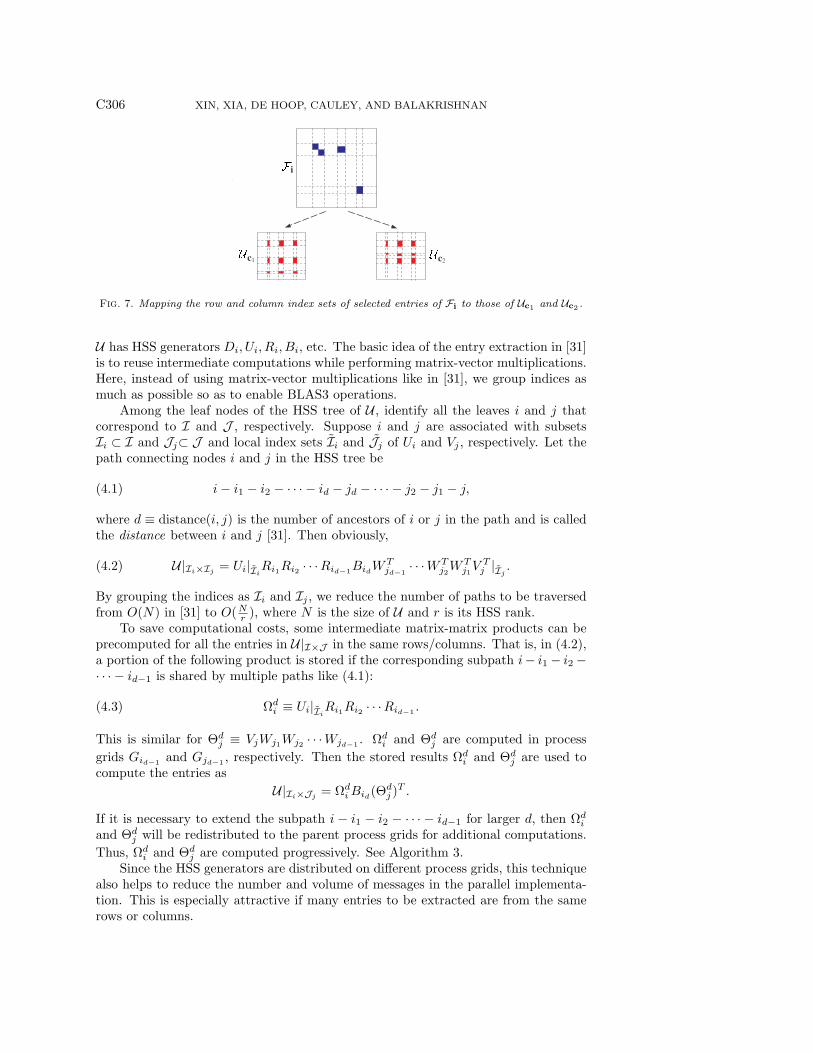
4.4. Extracting selected entries from HSS update matrices. The matrix-vector products Y i (and also Zi) obtained in the previous subsection are then usedto construct an HSS approximation to Fi. This still needs selected entries of Fi thatwill be used to form the B generators and leaf level D generators [24, 35]. Given therow and column index sets, we can extract the entries of Fi from F0

i , Uc1 , and Uc2 in(3.3). F0

i is immediately available, and we focus on Uc1 and Uc2 .The indices of the desired entries of Fi are mapped to those of Uc1 and Uc2

(Figure 7). Thus, we consider how to extract in parallel selected entries U|I×J of anHSS matrix U , as specified by a row index set I and a column index set J . Suppose


c1 c2

i

Fig. 7. Mapping the row and column index sets of selected entries of Fi to those of Uc1 and Uc2 .

U has HSS generators Di, Ui, Ri, Bi, etc. The basic idea of the entry extraction in [31]is to reuse intermediate computations while performing matrix-vector multiplications.Here, instead of using matrix-vector multiplications like in [31], we group indices asmuch as possible so as to enable BLAS3 operations.

Among the leaf nodes of the HSS tree of U , identify all the leaves i and j thatcorrespond to I and J , respectively. Suppose i and j are associated with subsetsIi ⊂ I and Jj⊂ J and local index sets Ii and Jj of Ui and Vj , respectively. Let thepath connecting nodes i and j in the HSS tree be

(4.1) i− i1 − i2 − · · · − id − jd − · · · − j2 − j1 − j,

where d ≡ distance(i, j) is the number of ancestors of i or j in the path and is calledthe distance between i and j [31]. Then obviously,

(4.2) U|Ii×Ij = Ui|IiRi1Ri2 · · ·Rid−1BidW

Tjd−1· · ·WT

j2WTj1V

Tj |Ij

.

By grouping the indices as Ii and Ij , we reduce the number of paths to be traversedfrom O(N) in [31] to O(Nr ), where N is the size of U and r is its HSS rank.

To save computational costs, some intermediate matrix-matrix products can beprecomputed for all the entries in U|I×J in the same rows/columns. That is, in (4.2),a portion of the following product is stored if the corresponding subpath i− i1− i2−· · · − id−1 is shared by multiple paths like (4.1):

(4.3) Ωdi ≡ Ui|IiRi1Ri2 · · ·Rid−1 .

This is similar for Θdj ≡ VjWj1Wj2 · · ·Wjd−1 . Ωdi and Θd

j are computed in processgrids Gid−1 and Gjd−1 , respectively. Then the stored results Ωdi and Θd

j are used tocompute the entries as

U|Ii×Jj= ΩdiBid(Θd

j )T .

If it is necessary to extend the subpath i − i1 − i2 − · · · − id−1 for larger d, then Ωdiand Θd

j will be redistributed to the parent process grids for additional computations.Thus, Ωdi and Θd

j are computed progressively. See Algorithm 3.Since the HSS generators are distributed on different process grids, this technique

also helps to reduce the number and volume of messages in the parallel implementa-tion. This is especially attractive if many entries to be extracted are from the samerows or columns.


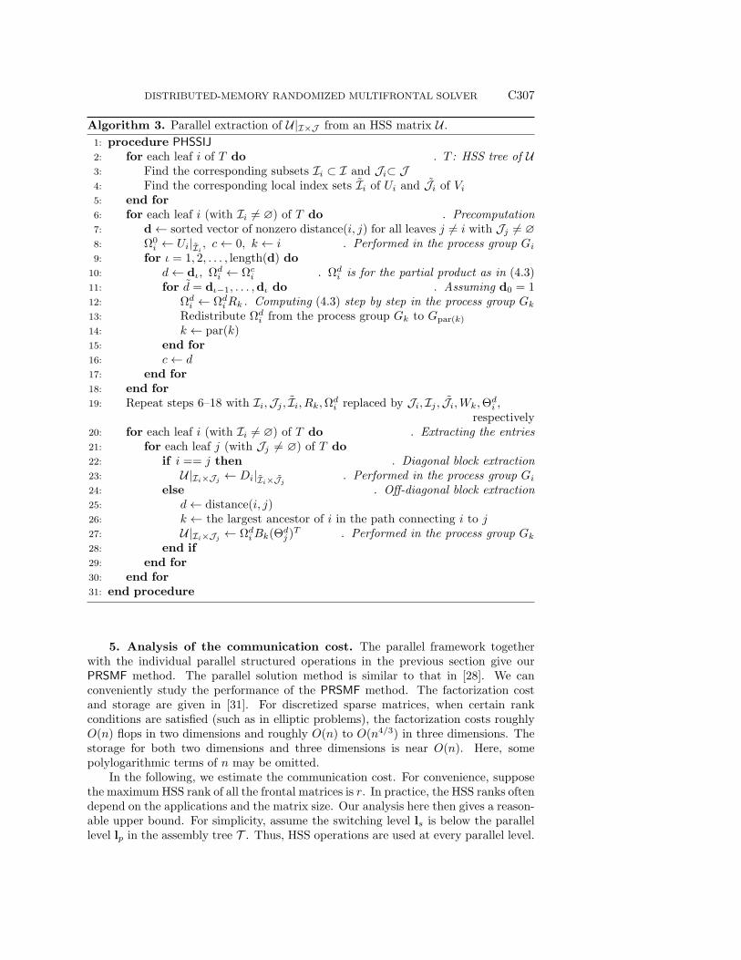
Algorithm 3. Parallel extraction of U|I×J from an HSS matrix U .1: procedure PHSSIJ2: for each leaf i of T do . T : HSS tree of U3: Find the corresponding subsets Ii ⊂ I and Ji⊂ J4: Find the corresponding local index sets Ii of Ui and Ji of Vi5: end for6: for each leaf i (with Ii 6= ∅) of T do . Precomputation7: d← sorted vector of nonzero distance(i, j) for all leaves j 6= i with Jj 6= ∅8: Ω0

i ← Ui|Ii, c← 0, k ← i . Performed in the process group Gi

9: for ι = 1, 2, . . . , length(d) do10: d← dι, Ωdi ← Ωci . Ωdi is for the partial product as in (4.3)11: for d = dι−1, . . . ,dι do . Assuming d0 = 112: Ωdi ← ΩdiRk . Computing (4.3) step by step in the process group Gk13: Redistribute Ωdi from the process group Gk to Gpar(k)14: k ← par(k)15: end for16: c← d17: end for18: end for19: Repeat steps 6–18 with Ii,Jj , Ii, Rk,Ωdi replaced by Ji, Ij , Ji,Wk,Θd

i ,respectively

20: for each leaf i (with Ii 6= ∅) of T do . Extracting the entries21: for each leaf j (with Jj 6= ∅) of T do22: if i == j then . Diagonal block extraction23: U|Ii×Jj ← Di|Ii×Jj

. Performed in the process group Gi24: else . Off-diagonal block extraction25: d← distance(i, j)26: k ← the largest ancestor of i in the path connecting i to j27: U|Ii×Jj ← ΩdiBk(Θd

j )T . Performed in the process group Gk

28: end if29: end for30: end for31: end procedure

5. Analysis of the communication cost. The parallel framework togetherwith the individual parallel structured operations in the previous section give ourPRSMF method. The parallel solution method is similar to that in [28]. We canconveniently study the performance of the PRSMF method. The factorization costand storage are given in [31]. For discretized sparse matrices, when certain rankconditions are satisfied (such as in elliptic problems), the factorization costs roughlyO(n) flops in two dimensions and roughly O(n) to O(n4/3) in three dimensions. Thestorage for both two dimensions and three dimensions is near O(n). Here, somepolylogarithmic terms of n may be omitted.

In the following, we estimate the communication cost. For convenience, supposethe maximum HSS rank of all the frontal matrices is r. In practice, the HSS ranks oftendepend on the applications and the matrix size. Our analysis here then gives a reason-able upper bound. For simplicity, assume the switching level ls is below the parallellevel lp in the assembly tree T . Thus, HSS operations are used at every parallel level.


Let P be the total number of processes, P be the minimum number of processwithin the process grids. The number of processes of each process grid at level l of Tis

Pl =P

2l−1 .

Suppose a process grid with Pl processes has O(√Pl) rows and columns. Also suppose

all the HSS generators of the structured frontal matrices are of sizes O(r)×O(r).We first review the communication costs of some basic operations. Use #messages

and #words to denote the numbers of messages and words, respectively.• For a k×k matrix, redistribution between a process grid and its parent process

requires #messages = O(1) and #words at most O(k2

P).

• On the same process grid with P processes, the multiplication of two O(r)×O(r) matrices costs #messages = O( rb ) and #words = O( r2√

P), where b is

the block size used in ScaLAPACK.Suppose a frontal matrix F is at level l of T and has size nl. F corresponds to a

process grid with Pl process. Then at level l of the HSS tree T for F , the number ofprocesses is Pl

2l−1 . The number of parallel levels of the HSS tree is O(logPl).To analyze the communication costs at the factorization stage, we investigate the

communication at each level l of the assembly tree.1. Randomized HSS construction and ULV factorization.

In [23], it is shown that both operations cost

#messages = O(r log2 Pl

), #words = O

(r2 log2 Pl√

P

).

2. Structured Schur complement computation and multiplication of the Schurcomplement and random vectors.For each process, the information is passed in a top-down order along theHSS tree. The major operations are matrix redistributions and multiplica-tions, since the additions on the same process grid involve no communication.The redistribution costs O(logPl) messages and O( r

2 logPl

P) words. The mul-

tiplications between HSS generators at each level cost O( rb ) messages andO( r2√

P) words. Thus

#messages = O(logPl) +O(logPl)∑l=1

O(rb

)= O

(rb

logPl

),

#words = O

(r2 logPl

P

)+O(logPl)∑l=1

O

(r2√P

)= O

(r2 logPl√

P

).

The sampling of the structured Schur complement is performed via HSSmatrix-vector multiplications. The communication costs are similar to theestimates above.

3. Skinny extend-add operation and redistribution of the skinny sampling ma-trices.The skinny matrices are of size O(nl) × O(r). Each process communicateswith processes in the same column on the process grid. Thus

#messages = O(√

Pl

), #words = O

(rnl

Pl

).


The redistribution of the skinny sampling matrices costs

#messages = O(1), #words = O

(rnl

P

).

4. Extracting selected entries from HSS matrices.For each process, the information is passed in a bottom-up order along anHSS tree. The major operations are matrix redistribution and multiplications.Similar to the communication costs of the structured Schur complement com-putation,

#messages = O (logPl) +O(logPl)∑l=1

O(r

b) = O(r logPl),

#words = O

(r2 logPl

P

)+O(logPl)∑l=1

O

(r2√P

)= O

(r2 logPl√

P

).

The total communication costs can be estimated by summing up the above costs.The total number of messages is

#messages =O(logP )∑

l=1

(O(√

Pl

)+O

(r log2 Pl

))= O

(√P)

+O(r log3 P

).

The total number of words is

#words =O(logP )∑

l=1

(O

(rnl

P

)+O

(r2 log2 Pl√

P

)),

which depends on specific forms of nl. For 2D and 3D problems, nl = O(√n/2bl/2c)

and O(n2/3/2bl/2c), respectively. Thus, the total number of words for 2D problems is

#words = O

(r√n

P

)+O

(r2 log3 P√

P

)and for 3D problems is

#words = O

(rn

23

P

)+O

(r2 log3 P√

P

).

In comparison, the parallel solver in [28] has communication costs of #messages =O(√P ) +O(r log3 P ) and

#words = O

(n

P

)+O

(r√n log2 P√P

)for 2D problems,

#words = O

(n

43

P

)+O

(rn

23 log2 P√P

)for 3D problems. In particular, the numbers of words of our new parallel solver are

smaller by factors of about O(√nr ) and O(n

23

r ), respectively.

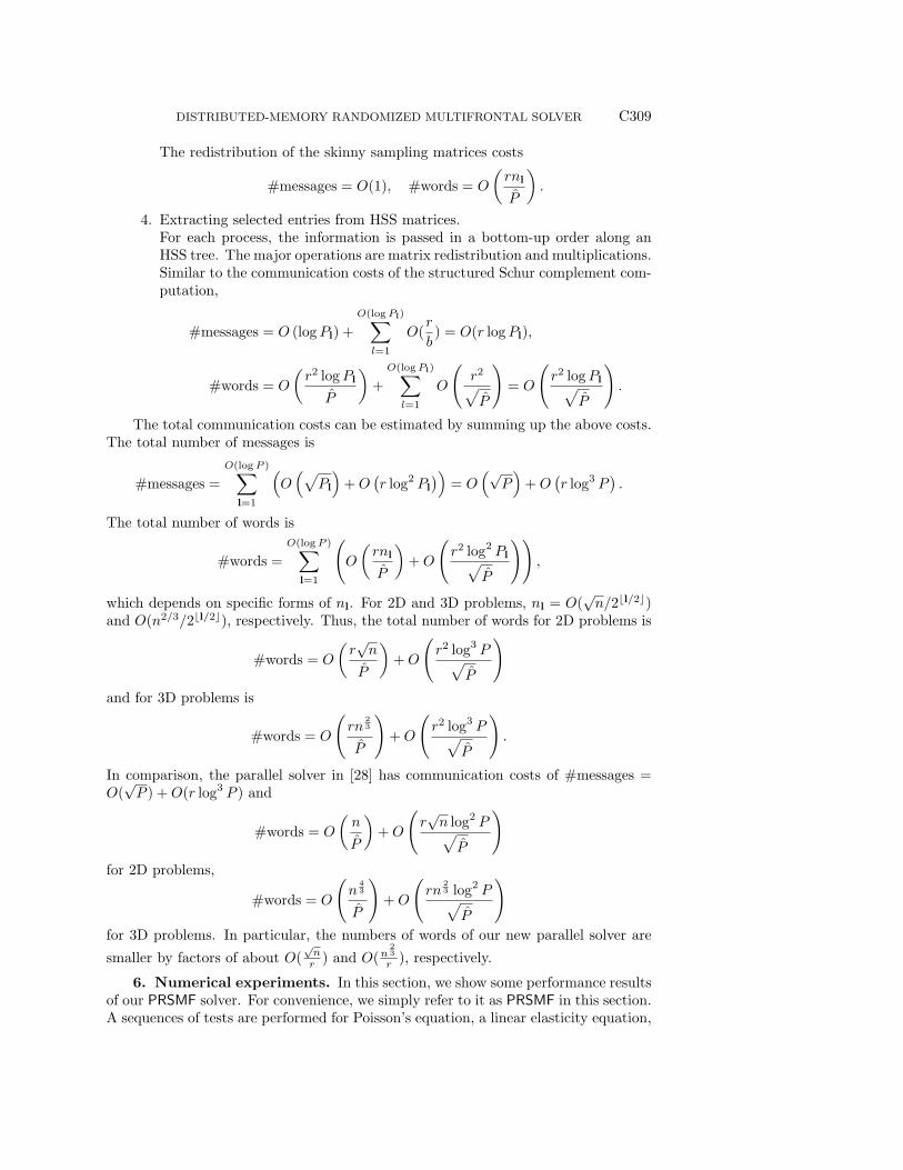
6. Numerical experiments. In this section, we show some performance resultsof our PRSMF solver. For convenience, we simply refer to it as PRSMF in this section.A sequences of tests are performed for Poisson’s equation, a linear elasticity equation,


Helmholtz equation, and a elastic wave equation in two or three dimensions. Wecarried out our experiments on a Cray XC30 cluster at TOTAL E&P Research &Technology USA. Each node has 20 cores and 64 GB memory. The number of nodesavailable for our tests is 52. The peak performance of each core is 23.30 Gflops. Weshow both the weak scalability and the strong scalability of the solver, as comparedwith the standard parallel multifrontal solver (by setting ls = 0 in PRSMF), denotedPMF. We report the following performance measurements:

• Time: the runtime for the factorization of A and the solution of Ax = b.• Flops and flop rate: the number of floating point operations in the factoriza-

tion and the corresponding flop rate.• Factor size: the number of nonzero entries for storing the factors.• Peak memory per process: the maximum memory occupied by one process

for any process.• Accuracy: the relative residual ||Ax−b||2||b||2 , where b is generated via a random

exact solution.In PRSMF, the maximum HSS rank of all the frontal matrices is also reported.

We also discuss how the variation of some parameters (the switching level and thesampling size) impacts the performance. In our current implementation, the numberof processes used is equal to 2lp−1, where lp is the parallel switching level. Thus, thestrong scaling tests below indicate the dependency of the code on lp. The followingnotation will be used for convenience:

• r: the sampling size in randomized compression (the column size of X in 3.5).• τ : the relative tolerance of rank-revealing factorizations of the matrix-vector

products as in (3.6).• lmax: the total number of levels in the assembly tree.

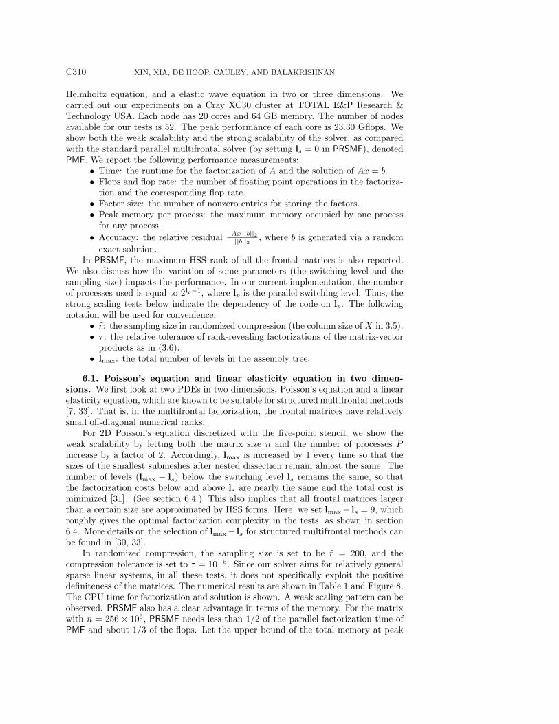
6.1. Poisson’s equation and linear elasticity equation in two dimen-sions. We first look at two PDEs in two dimensions, Poisson’s equation and a linearelasticity equation, which are known to be suitable for structured multifrontal methods[7, 33]. That is, in the multifrontal factorization, the frontal matrices have relativelysmall off-diagonal numerical ranks.

For 2D Poisson’s equation discretized with the five-point stencil, we show theweak scalability by letting both the matrix size n and the number of processes Pincrease by a factor of 2. Accordingly, lmax is increased by 1 every time so that thesizes of the smallest submeshes after nested dissection remain almost the same. Thenumber of levels (lmax − ls) below the switching level ls remains the same, so thatthe factorization costs below and above ls are nearly the same and the total cost isminimized [31]. (See section 6.4.) This also implies that all frontal matrices largerthan a certain size are approximated by HSS forms. Here, we set lmax− ls = 9, whichroughly gives the optimal factorization complexity in the tests, as shown in section6.4. More details on the selection of lmax− ls for structured multifrontal methods canbe found in [30, 33].

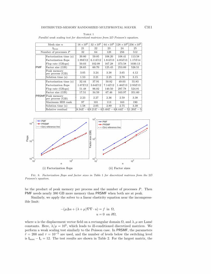
In randomized compression, the sampling size is set to be r = 200, and thecompression tolerance is set to τ = 10−5. Since our solver aims for relatively generalsparse linear systems, in all these tests, it does not specifically exploit the positivedefiniteness of the matrices. The numerical results are shown in Table 1 and Figure 8.The CPU time for factorization and solution is shown. A weak scaling pattern can beobserved. PRSMF also has a clear advantage in terms of the memory. For the matrixwith n = 256 × 106, PRSMF needs less than 1/2 of the parallel factorization time ofPMF and about 1/3 of the flops. Let the upper bound of the total memory at peak


Table 1Parallel weak scaling test for discretized matrices from 2D Poisson’s equation.

Mesh size n 16×106 32×106 64×106 128×106 256×106

lmax 21 22 23 24 25Number of processes P 32 64 128 256 512

PMF

Factorization time (s) 39.80 59.85 108.20 108.41 113.58Factorization flops 1.99E12 6.11E12 1.81E13 4.05E13 1.17E14Flop rate (Gflops) 50.03 102.09 167.28 373.58 1030.13Factor size (GB) 28.65 60.70 125.45 253.89 526.51Peak memory

3.05 3.24 3.38 3.65 4.12per process (GB)Solution time (s) 1.53 2.21 2.25 2.78 3.15

PRSMF


2.23 2.27 2.36 2.59 3.38per process (GB)Maximum HSS rank 97 101 113 163 190Solution time (s) 1.58 2.05 2.89 2.75 3.39Relative residual 8.34E − 6 9.21E − 6 5.48E − 6 8.44E − 5 1.20E − 5

107

108

1012

1013

1014

n

Flo

ps

PMF

PRSMF

O(n) reference line

107

108

101

102

103

n

Facto

r siz

e (

GB

)

PMF

PRSMF

O(n) reference line

(i) Factorization flops (ii) Factor sizes

Fig. 8. Factorization flops and factor sizes in Table 1 for discretized matrices from the 2DPoisson’s equation.

be the product of peak memory per process and the number of processes P . ThenPMF needs nearly 380 GB more memory than PRSMF when both are at peak.

Similarly, we apply the solver to a linear elasticity equation near the incompress-ible limit:

−(µ∆u+ (λ+ µ)∇∇ · u) = f in Ω,u = 0 on ∂Ω,

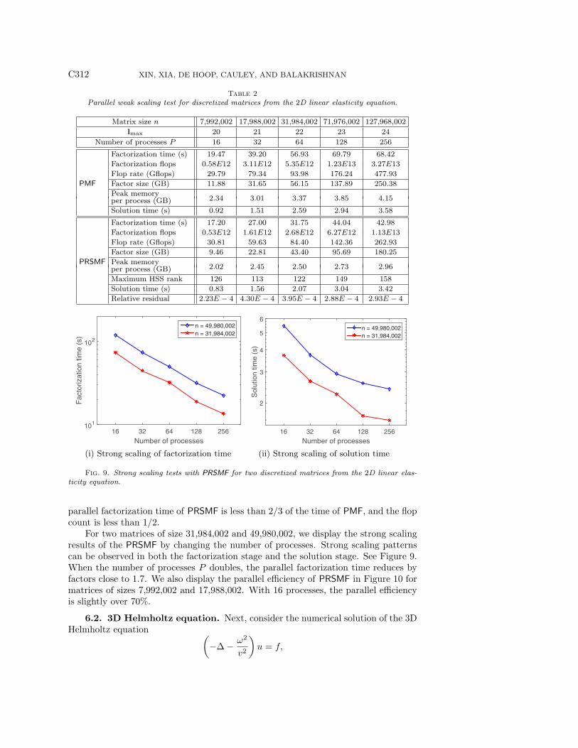
where u is the displacement vector field on a rectangular domain Ω, and λ, µ are Lameconstants. Here, λ/µ = 105, which leads to ill-conditioned discretized matrices. Weperform a weak scaling test similarly to the Poisson case. In PRSMF, the parametersr = 200 and τ = 10−5 are used, and the number of levels below the switching levelis lmax − ls = 12. The test results are shown in Table 2. For the largest matrix, the


Table 2Parallel weak scaling test for discretized matrices from the 2D linear elasticity equation.

Matrix size n 7,992,002 17,988,002 31,984,002 71,976,002 127,968,002lmax 20 21 22 23 24

Number of processes P 16 32 64 128 256

PMF


2.34 3.01 3.37 3.85 4.15per process (GB)Solution time (s) 0.92 1.51 2.59 2.94 3.58

PRSMF


2.02 2.45 2.50 2.73 2.96per process (GB)Maximum HSS rank 126 113 122 149 158Solution time (s) 0.83 1.56 2.07 3.04 3.42Relative residual 2.23E − 4 4.30E − 4 3.95E − 4 2.88E − 4 2.93E − 4

Number of processes

16 32 64 128 256

Fa

cto

riza

tio

n t

ime

(s)

101

102

n = 49,980,002

n = 31,984,002

Number of processes

16 32 64 128 256

So

lutio

n t

ime

(s)

2

3

4

5

6

n = 49,980,002

n = 31,984,002

(i) Strong scaling of factorization time (ii) Strong scaling of solution time

Fig. 9. Strong scaling tests with PRSMF for two discretized matrices from the 2D linear elas-ticity equation.

parallel factorization time of PRSMF is less than 2/3 of the time of PMF, and the flopcount is less than 1/2.

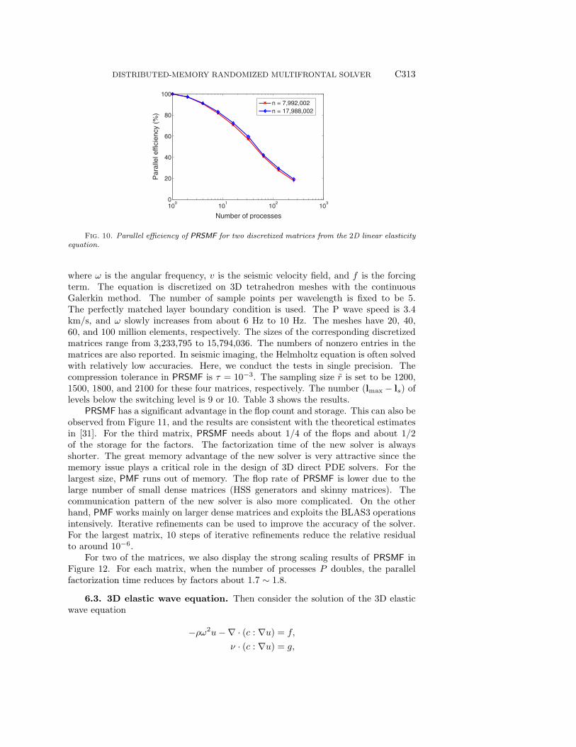
For two matrices of size 31,984,002 and 49,980,002, we display the strong scalingresults of the PRSMF by changing the number of processes. Strong scaling patternscan be observed in both the factorization stage and the solution stage. See Figure 9.When the number of processes P doubles, the parallel factorization time reduces byfactors close to 1.7. We also display the parallel efficiency of PRSMF in Figure 10 formatrices of sizes 7,992,002 and 17,988,002. With 16 processes, the parallel efficiencyis slightly over 70%.

6.2. 3D Helmholtz equation. Next, consider the numerical solution of the 3DHelmholtz equation (

−∆− ω2

v2

)u = f,


100

101

102

103

0

20

40

60

80

100

Number of processes

Para

llel effic

iency (

%)

n = 7,992,002

n = 17,988,002

Fig. 10. Parallel efficiency of PRSMF for two discretized matrices from the 2D linear elasticityequation.

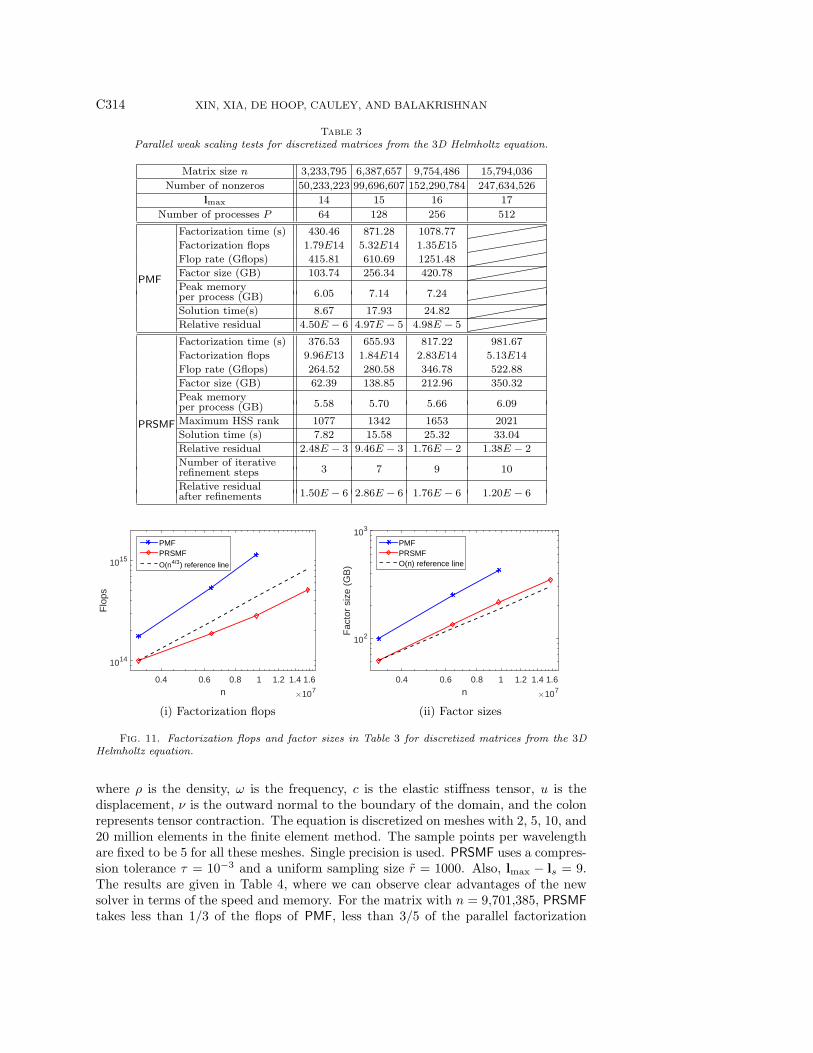
where ω is the angular frequency, v is the seismic velocity field, and f is the forcingterm. The equation is discretized on 3D tetrahedron meshes with the continuousGalerkin method. The number of sample points per wavelength is fixed to be 5.The perfectly matched layer boundary condition is used. The P wave speed is 3.4km/s, and ω slowly increases from about 6 Hz to 10 Hz. The meshes have 20, 40,60, and 100 million elements, respectively. The sizes of the corresponding discretizedmatrices range from 3,233,795 to 15,794,036. The numbers of nonzero entries in thematrices are also reported. In seismic imaging, the Helmholtz equation is often solvedwith relatively low accuracies. Here, we conduct the tests in single precision. Thecompression tolerance in PRSMF is τ = 10−3. The sampling size r is set to be 1200,1500, 1800, and 2100 for these four matrices, respectively. The number (lmax − ls) oflevels below the switching level is 9 or 10. Table 3 shows the results.

PRSMF has a significant advantage in the flop count and storage. This can also beobserved from Figure 11, and the results are consistent with the theoretical estimatesin [31]. For the third matrix, PRSMF needs about 1/4 of the flops and about 1/2of the storage for the factors. The factorization time of the new solver is alwaysshorter. The great memory advantage of the new solver is very attractive since thememory issue plays a critical role in the design of 3D direct PDE solvers. For thelargest size, PMF runs out of memory. The flop rate of PRSMF is lower due to thelarge number of small dense matrices (HSS generators and skinny matrices). Thecommunication pattern of the new solver is also more complicated. On the otherhand, PMF works mainly on larger dense matrices and exploits the BLAS3 operationsintensively. Iterative refinements can be used to improve the accuracy of the solver.For the largest matrix, 10 steps of iterative refinements reduce the relative residualto around 10−6.

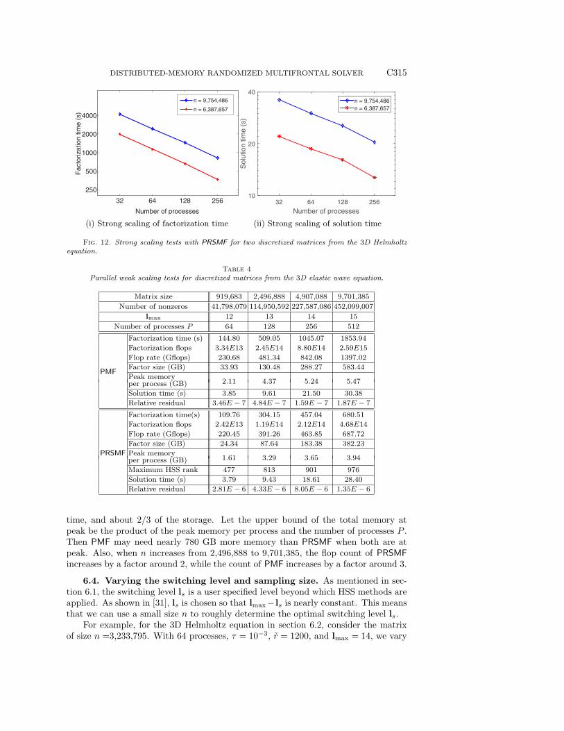
For two of the matrices, we also display the strong scaling results of PRSMF inFigure 12. For each matrix, when the number of processes P doubles, the parallelfactorization time reduces by factors about 1.7 ∼ 1.8.

6.3. 3D elastic wave equation. Then consider the solution of the 3D elasticwave equation

−ρω2u−∇ · (c : ∇u) = f,

ν · (c : ∇u) = g,


Table 3Parallel weak scaling tests for discretized matrices from the 3D Helmholtz equation.

Matrix size n 3,233,795 6,387,657 9,754,486 15,794,036Number of nonzeros 50,233,223 99,696,607 152,290,784 247,634,526

lmax 14 15 16 17Number of processes P 64 128 256 512

PMF

Factorization time (s) 430.46 871.28 1078.77Factorization flops 1.79E14 5.32E14 1.35E15Flop rate (Gflops) 415.81 610.69 1251.48Factor size (GB) 103.74 256.34 420.78Peak memory

6.05 7.14 7.24per process (GB)Solution time(s) 8.67 17.93 24.82Relative residual 4.50E − 6 4.97E − 5 4.98E − 5

PRSMF

Factorization time (s) 376.53 655.93 817.22 981.67Factorization flops 9.96E13 1.84E14 2.83E14 5.13E14Flop rate (Gflops) 264.52 280.58 346.78 522.88Factor size (GB) 62.39 138.85 212.96 350.32Peak memory

5.58 5.70 5.66 6.09per process (GB)Maximum HSS rank 1077 1342 1653 2021Solution time (s) 7.82 15.58 25.32 33.04Relative residual 2.48E − 3 9.46E − 3 1.76E − 2 1.38E − 2Number of iterative

3 7 9 10refinement stepsRelative residual

1.50E − 6 2.86E − 6 1.76E − 6 1.20E − 6after refinements

n ×107

0.4 0.6 0.8 1 1.2 1.4 1.6

Flo

ps

1014

1015

PMFPRSMF

O(n4/3) reference line

n ×107

0.4 0.6 0.8 1 1.2 1.4 1.6

Fac

tor

size

(G

B)

102

103

PMFPRSMFO(n) reference line


Fig. 11. Factorization flops and factor sizes in Table 3 for discretized matrices from the 3DHelmholtz equation.

where ρ is the density, ω is the frequency, c is the elastic stiffness tensor, u is thedisplacement, ν is the outward normal to the boundary of the domain, and the colonrepresents tensor contraction. The equation is discretized on meshes with 2, 5, 10, and20 million elements in the finite element method. The sample points per wavelengthare fixed to be 5 for all these meshes. Single precision is used. PRSMF uses a compres-sion tolerance τ = 10−3 and a uniform sampling size r = 1000. Also, lmax − ls = 9.The results are given in Table 4, where we can observe clear advantages of the newsolver in terms of the speed and memory. For the matrix with n = 9,701,385, PRSMFtakes less than 1/3 of the flops of PMF, less than 3/5 of the parallel factorization


32 64 128 256

250

500

1000

2000

4000

Number of processes

Facto

rization tim

e (

s)

n = 9,754,486

n = 6,387,657

Number of processes

32 64 128 256

So

lutio

n t

ime

(s)

10

20

40

n = 9,754,486

n = 6,387,657

(i) Strong scaling of factorization time (ii) Strong scaling of solution time

Fig. 12. Strong scaling tests with PRSMF for two discretized matrices from the 3D Helmholtzequation.

Table 4Parallel weak scaling tests for discretized matrices from the 3D elastic wave equation.

Matrix size 919,683 2,496,888 4,907,088 9,701,385Number of nonzeros 41,798,079 114,950,592 227,587,086 452,099,007

lmax 12 13 14 15Number of processes P 64 128 256 512

PMF

Factorization time (s) 144.80 509.05 1045.07 1853.94Factorization flops 3.34E13 2.45E14 8.80E14 2.59E15Flop rate (Gflops) 230.68 481.34 842.08 1397.02Factor size (GB) 33.93 130.48 288.27 583.44Peak memory

2.11 4.37 5.24 5.47per process (GB)Solution time (s) 3.85 9.61 21.50 30.38Relative residual 3.46E − 7 4.84E − 7 1.59E − 7 1.87E − 7

PRSMF

Factorization time(s) 109.76 304.15 457.04 680.51Factorization flops 2.42E13 1.19E14 2.12E14 4.68E14Flop rate (Gflops) 220.45 391.26 463.85 687.72Factor size (GB) 24.34 87.64 183.38 382.23Peak memory

1.61 3.29 3.65 3.94per process (GB)Maximum HSS rank 477 813 901 976Solution time (s) 3.79 9.43 18.61 28.40Relative residual 2.81E − 6 4.33E − 6 8.05E − 6 1.35E − 6

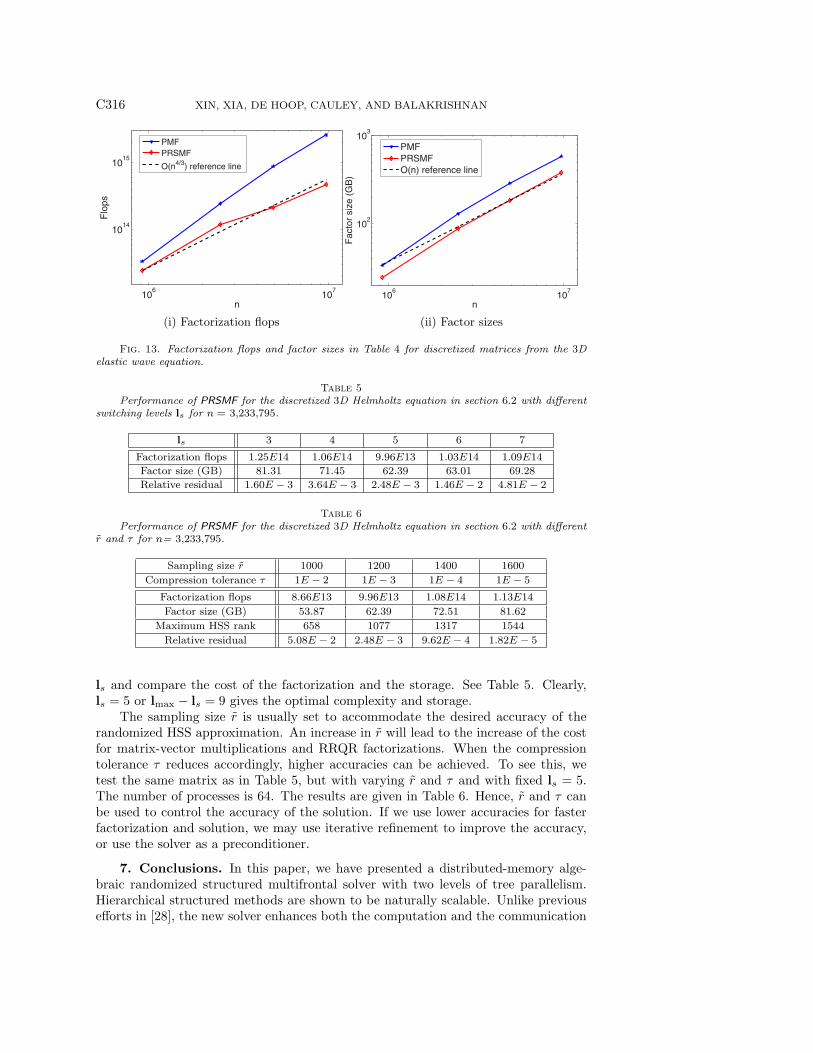
time, and about 2/3 of the storage. Let the upper bound of the total memory atpeak be the product of the peak memory per process and the number of processes P .Then PMF may need nearly 780 GB more memory than PRSMF when both are atpeak. Also, when n increases from 2,496,888 to 9,701,385, the flop count of PRSMFincreases by a factor around 2, while the count of PMF increases by a factor around 3.

6.4. Varying the switching level and sampling size. As mentioned in sec-tion 6.1, the switching level ls is a user specified level beyond which HSS methods areapplied. As shown in [31], ls is chosen so that lmax− ls is nearly constant. This meansthat we can use a small size n to roughly determine the optimal switching level ls.

For example, for the 3D Helmholtz equation in section 6.2, consider the matrixof size n =3,233,795. With 64 processes, τ = 10−3, r = 1200, and lmax = 14, we vary


106

107

1014

1015

n

Flo

ps

PMF

PRSMF

O(n4/3

) reference line

106

107

102

103

n

Facto

r siz

e (

GB

)

PMF

PRSMF

O(n) reference line


Fig. 13. Factorization flops and factor sizes in Table 4 for discretized matrices from the 3Delastic wave equation.

Table 5Performance of PRSMF for the discretized 3D Helmholtz equation in section 6.2 with different

switching levels ls for n = 3,233,795.

ls 3 4 5 6 7

Factorization flops 1.25E14 1.06E14 9.96E13 1.03E14 1.09E14Factor size (GB) 81.31 71.45 62.39 63.01 69.28Relative residual 1.60E − 3 3.64E − 3 2.48E − 3 1.46E − 2 4.81E − 2

Table 6Performance of PRSMF for the discretized 3D Helmholtz equation in section 6.2 with different

r and τ for n= 3,233,795.

Sampling size r 1000 1200 1400 1600Compression tolerance τ 1E − 2 1E − 3 1E − 4 1E − 5

Factorization flops 8.66E13 9.96E13 1.08E14 1.13E14Factor size (GB) 53.87 62.39 72.51 81.62

Maximum HSS rank 658 1077 1317 1544Relative residual 5.08E − 2 2.48E − 3 9.62E − 4 1.82E − 5

ls and compare the cost of the factorization and the storage. See Table 5. Clearly,ls = 5 or lmax − ls = 9 gives the optimal complexity and storage.

The sampling size r is usually set to accommodate the desired accuracy of therandomized HSS approximation. An increase in r will lead to the increase of the costfor matrix-vector multiplications and RRQR factorizations. When the compressiontolerance τ reduces accordingly, higher accuracies can be achieved. To see this, wetest the same matrix as in Table 5, but with varying r and τ and with fixed ls = 5.The number of processes is 64. The results are given in Table 6. Hence, r and τ canbe used to control the accuracy of the solution. If we use lower accuracies for fasterfactorization and solution, we may use iterative refinement to improve the accuracy,or use the solver as a preconditioner.

7. Conclusions. In this paper, we have presented a distributed-memory alge-braic randomized structured multifrontal solver with two levels of tree parallelism.Hierarchical structured methods are shown to be naturally scalable. Unlike previousefforts in [28], the new solver enhances both the computation and the communication


by using randomization to avoid dense intermediate matrices. It can also handle moregeneral matrices. Several parallel HSS algorithms have been developed for the solver.The solver achieves the desired complexity and shows nice scalability in testing somediscretized PDEs.

The implementation of this solver is relatively complex. It is built upon multiplecomponents such as multifrontal methods, HSS algorithms, and randomized methods.The efficient implementations of some components are extensively studied by thescientific computing community. Here, we build a systematic fast parallel structuredsparse solver, and also provide some new parallel implementations of several usefulstrategies in sparse and structured solutions. In the near future, we hope to makethe individual components and even the entire solver work as black-box codes so thatother researchers can conveniently use them for different tasks without knowing thetechnical details. Such codes will be made publicly available. It is also possible tosimplify the implementation using simpler structures such as the HODLR form [1].

Due to the complex scale of the project, no pivoting is integrated yet. Anotherreason for this is that it is not clear how pivoting affects the structures since thestructures depend on proper ordering. This will be thoroughly studied in futurework. Out future work will also include an adaptive scheme for choosing samplingsizes at different levels of the assembly tree, the replacement of intermediate HSSforms by multilayer structures [32], the use of batched BLAS for multiple small BLASoperations, as well as more extensive direct solution and preconditioning tests.

Acknowledgments. We thank Xiao Liu, Fabien Peyruss, and Jia Shi for helpingwith the numerical tests and thank TOTAL E&P Research & Technology USA forproviding the computing resource. We are also grateful to the three anonymousreferees for the valuable suggestions.

REFERENCES

[1] S. Ambikasaran and E. F. Darve, An O(N logN) fast direct solver for partial hierarchicallysemi-separable matrices, J. Sci. Comput., 57 (2013), pp. 477–501.

[2] P. Amestoy, C. Ashcraft, O. Boiteau, A. Buttari, J.-Y. L’Excellent, and C. Weis-becker, Improving multifrontal methods by means of block low-rank representations, SIAMJ. Sci. Comput., 37 (2015), pp. A1451–A1474.

[3] P. Amestoy, I. S. Duff, and J. Y. L’Excellent, Multifrontal parallel distributed symmetricand unsymmetric solvers, Comput. Methods Appl. Mech. Engrg. 184 (2000), pp. 501–520.

[4] L. S. Blackford, J. Choi, A. Cleary, E. D’Azeuedo, J. Demmel, I. Dhillon, et al.,ScaLAPACK User’s Guide, SIAM, Philadelphia, PA, 1997.

[5] S. Borm and W. Hackbusch, Data-sparse approximation by adaptive H2-matrices, Comput-ing, 69 (2002), pp. 1–35.

[6] S. Chandrasekaran, P. Dewilde, M. Gu, and T. Pals, A fast ULV decomposition solverfor hierarchically semiseparable representations, SIAM J. Matrix Anal. Appl., 28 (2006),pp. 603–622.

[7] S. Chandrasekaran, P. Dewilde, M. Gu, and N. Somasunderam, On the numerical rank ofthe off-diagonal blocks of Schur complements of discretized elliptic PDEs, SIAM J. MatrixAnal. Appl. 31 (2010), pp. 2261–2290.

[8] R. Clint Whaley, Basic Linear Algebra Communication Subprograms: Analysis and Imple-mentation Across Multiple Parallel Architectures, LAPACK Working Note 73, Universityof Tennessee, 1994.

[9] I. S. Duff and J. K. Reid, The multifrontal solution of indefinite sparse symmetric linear,ACM Trans. Math. Software, 9 (1983), pp. 302–325.

[10] J. A. George, Nested dissection of a regular finite element mesh, SIAM J. Numer. Anal., 10(1973), pp. 345–363.

[11] J. A. George, J. W. H. Liu, and E. Ng, Communication results for parallel sparse Choleskyfactorization on a hypercube, Parallel Comput., 10 (1989), pp. 287–298.

[12] N. Gibbs, W. Poole, and P. Stockmeyer, An algorithm for reducing the bandwidth andprofile of a sparse matrix, SIAM J. Sci. Comput., 13 (1976), pp. 236–250.


[13] J. R. Gilbert and S.-H. Teng, MESHPART, A MATLAB Mesh Partitioning and GraphSeparator Toolbox, http://aton.cerfacs.fr/algor/Softs/MESHPART.

[14] A. Gillman and P. G. Martinsson, A direct solver with O(N) complexity for variable co-efficient elliptic PDEs discretized via a high-order composite spectral collocation method,SIAM J. Sci. Comput., 36 (2014), pp. A2023–A2046.

[15] L. Grasedyck, R. Kriemann, and S. Le Borne, Domain-decomposition based H-LU pre-conditioners, in Domain Decomposition Methods in Science and Engineering XVI, O. B.Widlund and D. E. Keyes, eds., Lect. Notes. Comput. Sci. Eng. 55, Springer, New York,2006, pp. 661–668.

[16] M. Gu and S. C. Eisenstat, Efficient algorithms for computing a strong-rank revealing QRfactorization, SIAM J. Sci. Comput., 17 (1996), pp. 848–869.

[17] W. Hackbusch, B. N. Khoromskij, and R. Kriemann, Hierarchical matrices based on a weakadmissibility criterion, Computing, 73 (2004), pp. 207-243.

[18] N. Halko, P.G. Martinsson, and J. Tropp, Finding structure with randomness: Probabilisticalgorithms for constructing approximate matrix decompositions, SIAM Rev., 53 (2011),pp. 217–288.

[19] G. Karypis and V. Kumar, A fast and high quality multilevel scheme for partitioning irregulargraphs, SIAM J. Sci. Comput., 20 (1998), pp. 359–392.

[20] X. S. Li and J. W. Demmel, SuperLU DIST A scalable distributed-memory sparse direct solverfor unsymmetric linear systems, ACM Trans. Math. Software, 29, (2002), pp. 110–140.

[21] E. Liberty, F. Woolfe, P. G. Martinsson, V. Rokhlin, and M. Tygert, Randomizedalgorithms for the low-rank approximation of matrices, Proc. Natl. Acad. Sci. USA, 104(2007), pp. 20167–20172.

[22] J. W. H. Liu, The multifrontal method for sparse matrix solution: Theory and practice, SIAMRev., 34 (1992), pp. 82–109.

[23] X. Liu, J. Xia, and M. V. de Hoop, Parallel randomized and matrix-free direct solvers forlarge structured dense linear systems, SIAM J. Sci. Comput., 38, (2016), pp. S508–S538.

[24] P. G. Martinsson, A fast randomized algorithm for computing a hierarchically semiseparablerepresentation of a matrix, SIAM. J. Matrix Anal. Appl., 32 (2011), pp. 1251–1274.

[25] F. Pellegrini and J. Roman, Sparse matrix ordering with SCOTCH, in Proceedings ofHPCN’97, Vienna, Austria, Lecture Notes in Comput. Sci. 1225, Springer, New York,1997, pp. 370–378.

[26] A. Pothen and C. Sun, A mapping algorithm for parallel sparse Cholesky factorization, SIAMJ. Sci. Comput., 14 (1993), pp. 1253–1257.

[27] P. Schmitz and L. Ying, A fast direct solver for elliptic problems on general meshes in 2D,J. Comput. Phys., 231 (2012), pp. 1314–1338.

[28] S. Wang. X. S. Li, F. H. Rouet, J. Xia, and M. V. de Hoop, A parallel geometric multifrontalsolver using hierarchically semiseparable structure, ACM Trans. Math. Software, 42 (2016).

[29] S. Wang, X. S. Li, J. Xia, Y. Situ, and M. V. de Hoop, Efficient scalable algorithms forsolving dense linear systems with hierarchically semiseparable structures, SIAM J. Sci.Comput., 35 (2013), pp. C519–C544.

[30] J. Xia, Efficient structured multifrontal factorization for general large sparse matrices, SIAMJ. Sci. Comput., 35 (2013), pp. A832–A860.

[31] J. Xia, Randomized sparse direct solvers, SIAM J. Matrix Anal. Appl., 34 (2013), pp. 197–227.[32] J. Xia, Multilayer Hierarchically Semiseparable Structures, GMIG Report 15–16, Purdue Uni-

versity, 2015.[33] J. Xia, S. Chandrasekaran, M. Gu, and X. S. Li, Superfast multifrontal method for

large structured linear systems of equations, SIAM J. Matrix Anal. Appl., 31 (2009),pp. 1382–1411.

[34] J. Xia, S. Chandrasekaran, M. Gu, and X. S. Li, Fast algorithms for hierarchically semisep-arable matrices, Numer. Linear Algebra Appl., 17 (2010), pp. 953–976.

[35] J. Xia, Y. Xi, and M. Gu, A superfast structured solver for Toeplitz linear systems via ran-domized sampling, SIAM J. Matrix Anal. Appl., 33 (2012), pp. 837–858.

[36] Z. Xin, J. Xia, M. V. de Hoop, S. Cauley, and V. Balakrishnan, Parallel RandomizedStructured Multifrontal Method for General Sparse Matrices, GMIG Report 14–17, PurdueUniversity, 2014.

[37] Z. Xin, J. Xia, M. V. de Hoop, S. Cauley, and V. Balakrishnan, Scalable RandomizedStructured Multifrontal Method for Large-Scale Sparse Direct Solutions, GMIG Report15–14, Purdue University, 2015.

[38] Z. Xin, J. Xia, M. V. de Hoop, S. Cauley, and V. Balakrishnan, A Distributed-MemoryRandomized Structured Multifrontal Method for Sparse Direct Solutions, GMIG Report 9,Rice University, 2016, pp. 169–189.

a distributed-memory randomized structured multifrontal ...xiaj/work/mfpar.pdf · a...

Documents