A Distributed Path Query Engine forTemporal Property Graphs *

Shriram Ramesh, Animesh Baranawal and Yogesh SimmhanDepartment of Computational and Data Sciences,

Indian Institute of Science, Bangalore 560012, IndiaEmail: shriramr, animeshb, simmhan@iisc.ac.in

Abstract

Property graphs are a common form of linked data, with pathqueries used to traverse and explore them for enterprise transactionsand mining. Temporal property graphs are a recent variant where timeis a first-class entity to be queried over, and properties and structurevarying over time. These are seen in social, telecom and transit net-works. However, current graph databases and query engines have lim-ited support for temporal relations among graph entities, no supportfor time-varying entities and/or do not scale on distributed resources.We address this gap by extending a linear path query model over prop-erty graphs to include intuitive temporal predicates that operate overtemporal graphs. We design a distributed execution model for thesetemporal path queries using the interval-centric computing model, anddevelop a novel cost model to select an efficient execution plan fromseveral. We perform detailed experiments of our Granite distributedquery engine using temporal property graphs as large as 52M vertices,218M edges, and 118M properties, and a 800-query workload, derivedfrom the LDBC benchmark. We offer sub-second query latencies inmost cases, which is 154×–1786× faster compared to industry-leadingNeo4J shared-memory graph database and the JanusGraph/Spark dis-tributed graph query engine. Further, our cost model selects a queryplan that is within 10% of the optimal execution time in 90% of thecases. We also scale well, and complete 100% of the query workloadfor all graphs, as opposed to only 32–90% completion by the baselinesystems.

1 IntroductionGraphs are a natural model to represent and analyze linked data in vari-ous domains. Property graphs allow vertices and edges to have associated

*To appear in the Proceedings of the 20th IEEE/ACM International Symposium onCluster, Cloud and Internet Computing (CCGrid), Melbourne, Australia, May, 2020.

1

arX

iv:2

002.

0327

4v1

[cs

.DC

] 9

Feb

202

0

Alice Don

Pic Post

Bob[40, 60) [10, 30)

[30, 90)

[25, 100)

[0, 90)

[20, 100)

[5, 100)[35, 70)

Cleo

[50, 100)

[60, 70)

[20, 100) Tag: Vacation[20, 100) Country: India

[10, 100)

[10,80) Country: UK[80,90) Country: US[10,100) Gender: F

Likes

Follows

[5,100) Tag: Hiking

Figure 1: Sample Temporal Property Graph

key–value pair properties, besides the graph structure. This forms a rich in-formation schema and has been used to capture knowledge graphs (concepts,relations) [1], social networks (person, forum, message) [2], and financial andretail transactions (person, store, product) [3].

Path queries are a common query-class over property graphs [4,5].Here,the user defines a sequence of predicates over vertices and edges that shouldmatch along a path in the graph. E.g., in the property graph in Fig. 1,“[EQ1] Find a person (vertex type) who lives in ‘UK’ (vertex property)and follows (edge type) a person who follows another person who is taggedwith ‘Hiking’ (vertex property)” is a 3-hop path query, and would matchCleo→Alice→Bob, if we ignore the time intervals. Path queries are used toidentify concept pathways in knowledge graphs, fake news in social media,and product suggestions in retail websites. They also need to be performedrapidly, within 1 sec, as part of transactional requests from websites orexploratory queries by analysts.

While graph databases are designed for transactional read and writeworkloads, we consider graphs that are updated infrequently but queriedoften. For these workloads, graph query engines load and retain propertygraphs in-memory to service requests with low latency, without the needfor locking or consistency protocols [6]. Property graphs can be large, with105–108 vertices and edges, and 10’s of properties on each vertex or edge.This can exceed the memory on a single machine, often dominated by theproperties. This necessitates the use of distributed systems to scale to largegraphs.Challenges. Time is an increasingly common graph feature in a varietyof domains. However, existing property graph models fail to consider it asa first-class entity. Here, we distinguish between graphs with a time or alifespan associated with their entities (properties, vertices, edges), and thosewhere the entities themselves change over time and the history is available.

2

We call the former static temporal graphs and the latter dynamic temporalgraphs. E.g., in Fig. 1, the vertices, edges and properties have a lifespan,forming a temporal graph. Other than the properties of Cleo, the rest forma static temporal graph. But the Country property of Cleo changes overtime, causing it to be a dynamic temporal graph.

This gap is reflected not just in the data model but also in the queriessupported. Treating time as just another property fails to express tem-poral relations such as ensuring time-ordering among the entities on thepath. E.g., [EQ2] find people tagged with ‘Hiking’ who liked a post taggedas ‘Vacation’, before the post was liked by a person named ‘Don’, and [EQ3]find people who started to follow another person, after they stopped follow-ing ‘Don’. While these should match the paths Bob→PicPost→Don andAlice→Bob→Don, respectively, such queries are hard, if not impossible, toexpress in current graph databases. This motivates the need to supportintuitive temporal predicates to concisely express such temporal relations.

Further, existing graph databases and query engines do not support pathqueries over dynamic temporal graphs. E.g., the query EQ1 above shouldnot match Cleo→Alice→Bob since at the time Cleo was living in ‘UK’, shewas not following Alice. While platforms can be adapted to support queriesover graphs at a fixed time-point, temporal relationship over time-varyingproperties and structures cannot be expressed meaningfully. The scalabilityof existing graph systems is also limited.

We make the following specific contributions in this paper:• We propose a temporal property graph model, and intuitive temporalpredicates for path queries over them (§3).

• We design a distributed execution model for these queries using theinterval-centric computing model (§4).

• We develop a novel cost model that uses graph statistics to select thebest from multiple execution plans (§5).

• We evaluate the performance and scalability of Granite for 5 temporalgraphs and up to 800 queries, derived from the LDBC benchmark. Wecompare this against three configurations of Neo4J, and JanusGraphwhich uses Spark (§6).

Further, we discuss related work in Sec. 2 and offer our conclusions inSec. 7.

2 Related Work

2.1 Distributed and Temporal Graph Processing

There are several distributed graph processing platforms for running graphalgorithms on commodity clusters and clouds [7]. These typically offer pro-

3

gramming abstractions like Google Pregel’s vertex-centric computing model [8]and its component centric variants [9, 10] to design algorithms such asBreadth First Search, centrality scores and mining [11]. These execute us-ing a Bulk Synchronous Parallel (BSP) model, and scale to large graphs andapplications that explore the entire graph. They offer high throughput batchprocessing that take O(mins)–O(hours). We instead focus on exploratoryand transactional path queries that need to be processed in O(secs). Thisrequires careful use of existing distributed graph platforms and additionaloptimizations for fast responses.

There are also parallel graph platforms for HPC clusters [12]. Theseoptimize the memory and communication access to scale to graphs withbillions of entitles on thousands of cores [13]. They focus on high-throughputgraph algorithms. We instead target commodity hardware and cloud VMswith 10’s of nodes and 100’s of total cores, and are more accessible. We alsoaddress queries over temporal property graphs.

A few distributed platforms support high throughput temporal graphprocessing, with abstractions for designing temporal algorithms [14,15]. Weuse one such in-house system, Graphite, which extends Apache Giraph, asthe base framework for implementing our low-latency Granite path queryengine [16]. There are also a few platforms that support incremental com-puting as graph updates continuously arrive [17, 18]. We instead focus onproperty graphs with temporal lifespans on their vertices, edges and prop-erties that have already been collected in the past. In future, we plan toconsider incremental query processing over such dynamic graphs.

2.2 Property and Temporal Graph Querying

Query models over property graphs and associated query engines have beenpopular for semantic graphs [19,20]. Languages like SPARQL offer a highlyflexible declarative syntax, but are costly to execute in practice for largegraphs. Others support a narrower set of declarative query primitives, suchas finding paths, reachability and patterns over property graphs, but man-age to scale to large graphs using a distributed execution model [21, 22].However, none of these support time as a first-class entity, either duringquery specification or during execution.

There has been limited work on querying and indexing over specific tem-poral features of property graph. [23] propose a model for finding the top-kgraph patterns which exist for longest period of time over a series of graphsnapshots. The propose several indexing techniques to minimize the snap-shot search space, and perform a brute-force pattern mining on the restrictedset. This multi-snapshot approach limits the pattern to fully exist at a singletime point and recur across time, rather than allow it to span time intervals.It is also limited to a single-machine execution, which limits scaling.

TimeReach [24] supports conjunctive and disjunctive reachability queries

4

on a series of temporal graph snapshot. It builds an index from strongly con-nected components (SCC) for each snapshot, condenses them across time,and use this to traverse between vertices in different SCCs within a sin-gle hop assuming that the graph has few SCCs that do not change muchover time. They also require the path to be reachable within a single snap-shot rather than allow path segments to connect across time. Likewise,TopChain [25] supports temporal reachability query using an index label-ing scheme. It unrolls the temporal graph into a static graph, with timeexpanded as additional edges, finds the chain-cover over it, and stores thetop-k reachable chains from each vertex as labels. It uses this to answertime-respecting reachability, earliest arrival path and fastest path queries.Paths can span time intervals. However, they do not support any predicatesover the properties. Neither of these support distributed execution.

ChronoGraph [26] supports temporal path traversal queries over intervalproperty graphs. They implement this using the Gremlin property graphquery language over TinkerGraph engine. They propose a set of optimiza-tions to the Gremlin traversal operators, offer parallelization and lazy traver-sals within a single machine. However, they do not design or use any in-dexing structures or statistics to make the execution plan efficient. Theiroptimizations are also tightly-coupled to the execution engine, which itselfis deprecated and does not support distributed execution.

In summary, these various platforms and techniques lack one or moreof the following capabilities that we offer: modeling time as a first-classgraph and query concept, besides properties and enabling temporal pathqueries that allow the path to span time and match temporal relations acrossentities; a distributed execution model on commodity clusters, that scales tolarge graphs using a query cost optimizer based on statistics over the graph.

3 Temporal Graph and Query Models

3.1 Temporal Concepts

The temporal property graph concepts used in this paper are drawn fromour earlier work [16]. Time is a linearly ordered discrete domain Ω whoserange is the set of non-negative whole numbers. Each instant in this domainis called a time-point and an atomic increment in time is called a time-unit.A time interval is given by τ = [ts, te) where ts, te ∈ Ω which indicatesan interval starting from and including ts and extends to but excludes te.Interval relations [27] are boolean comparators between intervals; fully beforerelation is denoted by , starts before relation by ≺, fully after relation by, starts after relation by , and overlaps relation by u.

5

3.2 Temporal Property Graph Model

We formally define a temporal property graph as a directed graph G =(V,E, PV , PE). V is a set of typed vertices where each vertex 〈vid, σ, τ〉 ∈ Vis a tuple with a unique vertex ID, vid, a vertex type (or schema) σ, andthe lifespan of existence of the vertex given by the interval, τ = [ts, te). Eis a set of directed typed edges, with 〈eid, σ, vidi, vidj , τ〉 ∈ E. Here, eid isa unique ID of the edge, σ its type, vidi and vidj are its source and sinkvertices, respectively, and τ = [ts, te) is its lifespan. We have a schemafunction S : σ → K, that maps a given vertex or edge type σ to the set ofproperty keys (or names) it can have. PV is a set of vertex property values,where each 〈vid, κ, val, τp〉 ∈ PV represents a value for the key κ ∈ K for thevertex vid, with the value valid for the interval τp ∈ τ . Similar definitionapplies for edge property 〈eid, κ, val, τp〉 ∈ PE .

Further, the graph G must meet the uniqueness constraint of verticesand edges, referential integrity constraints, and constant edge associationconstraints [28].

A static temporal property graph is a restricted version of the temporalproperty graph such that τp = τ for the vertex and edge properties, i.e.,each property key has a static value that is valid for the entire vertex oredge lifespan. Graphs without this restriction are called dynamic temporalproperty graphs, and these allow keys for a vertex or an edge to have differentvalues for non-overlapping time intervals. E.g., omitting vertex Cleo in Fig. 1makes it a static property graph, but retaining it makes this a dynamicproperty graph.

3.3 Temporal Path Query

An n-hop linear chain path query is a pattern matching query with n vertexpredicates and n− 1 edge predicates. The syntax rules for this query modeland its predicates are given below.

〈path〉 ::= 〈ve-path〉* 〈v-pred〉

〈ve-path〉 ::= 〈v-pred〉 ` 〈e-pred〉| 〈v-pred〉 ` 〈e-pred〉 〈vint-pred〉 ` 〈e-pred〉

〈vint-pred〉 ::= 〈v-pred〉 | 〈v-pred〉 〈etr-clause〉

〈v-pred〉 ::= 〈pred〉

〈e-pred〉 ::= 〈pred〉 〈direction〉

〈dir〉 ::= → | ← | ↔

〈pred〉 ::= ? | 〈bol-pred〉 |〈prop-clause〉|〈time-clause〉

〈bol-pred〉 ::= 〈prop-clause〉 | 〈prop-clause〉OR〈bol-pred〉| 〈prop-clause〉AND〈bol-pred〉

6

〈prop-clause〉 ::= ve-key 〈prop-comp〉 value

〈time-clause〉 ::= ve-lifespan 〈time-comp〉 interval

〈etr-clause〉 ::= el-lifespan〈time-comp〉er-lifespan

〈prop-comp〉 ::= ‘==’ | ‘!=’ | ⊂

〈time-comp〉 ::= ≺ | | | | u | 6 u

As we can see, the property and time clauses are the atomic elements ofthe predicate and allow in/equality and containment comparison betweena property key and the given value, and a more flexible set of comparisonsbetween a vertex/edge/property lifespan and a given interval. These tem-poral clauses allow a wide variety of comparison within the context of asingle vertex or edge, and their properties. These clauses can be combinedusing Boolean AND and OR operators. Edge predicates can have an optionaldirection. The wildcard ? matches all vertices or edges at a hop.

A novel and powerful temporal operator we introduce is edge time re-lationship (ETR). Unlike the time clause, this etr-clause allows comparisonacross entities. Specifically, it is defined on an intermediate vertex in thepath (vint-pred), and allows us to compare the lifespans of the left (el-lifespan) and right (er-lifespan) edges. The motivation for this operatorcomes from social network mining [5] and to identify flow and frauds intransactions networks [3]. E.g., EQ2 and EQ3 from Sec. 1 can be capturedusing this.

4 Distributed Query Engine

4.1 Relaxed Interval Centric Computing

Our query engine uses a distributed in-memory iterative execution modelthat extends and relaxes the interval centric computing model (ICM) [16].ICM adds a temporal dimension to Pregel’s vertex centric iterative com-puting model [8]. Users define their computation from the perspective ofa single interval-vertex, i.e., the state and properties for a certain intervalof a vertex’s lifespan. In each iteration (superstep) of an ICM application,a user-defined compute function is called on each active interval-vertex,which operates on its prior state and on messages it receives from its neigh-bors, for that interval, and updates the current state. Then, a user-definedscatter function is called on that interval-vertex that allows it to sendtemporal messages containing, say, the updated state to its neighbors alongthe out edges. The message lifespan is typically the intersection of the inter-val state and the edge lifespan. All active interval-vertices in the distributedgraph can execute in a data parallel manner in an iteration. Messages aredelivered in bulk at a barrier after the scatter phase, and the compute phase

7

VCM on Graph Apache GiraphICM on Interval Property Graph Graphite

Gra

nit

e

Worker

Master

Init/ Compute

(Resume) vertex

predicate evaluation.

ScatterEvaluate edge

predicate, temporal edge relation.

Send partial results message to sink vertex.

Master .

Receive & broadcast query to worker ◊ Select query plan using cost model ◊ Coordinate worker exec. for query plan ◊ Return result set to client

StatsOptimizer

Worker Worker Worker

MessagingControls

Qu

ery

HDFS

Figure 2: Architecture of Granite

for the next iteration starts after that. Vertices receiving a message whoseinterval overlaps with its lifespan are activated for the overlapping period.This repeats across supersteps until no messages are generated after a su-perstep.

We design our engine, called Granite, using the compute and scatterprimitives offered the Graphite implementation of ICM over Apache Giraph.However, ICM enforces time-respecting behavior. Here, the intervals be-tween the messages and the interval-vertex state has to overlap for computeto be called, between updated interval states by the compute and the edgelifespans have to overlap for scatter to be called, and scatter sends messageson edges whose lifespan overlaps with the updated states. But the temporalpath queries do not need to meet these requirements. E.g., navigating fromvertex that occurs after an adjacent vertex is not allowed. Also, ICM uses aTimeWarp operator that allows messages and state intervals to be alignedto enforce this time-respecting behavior, but this operator is costly. So werelax ICM to allow non-time respecting behavior between compute, scatterand messaging, while leveraging other interval centric properties it offers.

4.2 Distributed Execution Model

In our execution model, each vertex predicate for a path query and thesucceeding edge predicate, if any, are evaluated in a single ICM superstep.Specifically, the vertex predicates are evaluated in the compute functionand the edge predicates in the scatter function. We use a specializedlogic called init for the first vertex predicate in a query.

8

4.2.1 Execution over Static Temporal Graphs

A master receives the path query from the client, and broadcasts it to allworkers to start the first superstep. Each worker operates over a set of graphpartitions with a single thread per partition, and each thread is responsiblefor calling the compute and scatter functions on every active vertex in itspartition. The init logic is called on all vertices in the first superstep.It resets the vertex state for this new query and evaluates the first vertexpredicate of the query. If vertex matches, its state is updated with a matchflag and scatter is invoked for each of its incident (in/out) edges. Scatterevaluates the next edge predicate, and if it matches, sends the partial pathresult to the destination vertex as a message, along with the evaluated pathlength. If a match fails, this path traversal is pruned.

In the next iteration, our compute logic is called for vertices receivinga message. This evaluates the next vertex predicate in the path and if itmatches, it puts all the partial path results from the input messages in thevertex state, and scatter is called on each incident edge. If the edge matchesthe next edge predicate, the current vertex and edge are appended to eachprior partial result and sent to the destination vertex. This continues foras many supersteps as the path length. In the last superstep, the verticeshaving the matching paths from their messages send it to the master toreturn back to the client.

Scatter also evaluates the edge temporal relationship. Here, the scatterof the preceding edge passes its lifespan as part of the result message, andthis is compared against the current edge’s lifespan by the next scatter todecide on a match.

For static temporal graphs, we do not use any interval-centric featuresof ICM, and the entire lifespan of the vertex is treated as a single interval-vertex for execution, and likewise for edges. However, we do use the propertygraph model and state management APIs offered by the interval-vertex.

4.2.2 Execution over Dynamic Temporal Graphs

For graphs with time varying properties, we leverage the interval-centricfeatures of ICM. Specifically, we enable TimeWarp of message intervals withthe vertex properties’ lifespans so that compute is called on an intervalvertex with messages temporally aligned and grouped against the propertyintervals. Scatter is called only for edges whose lifespans overlap with thematching interval-vertex, and its scope is limited to the period of overlap.The compute or scatter functions only access messages and propertiesthat are relevant to their current interval of relevance, and both can becalled multiple times, for different intervals, on the same vertex and edge.

9

4.3 Distributed Execution Plans

Queries can be evaluated by splitting them into smaller path query segmentsthat are independently evaluated and the results then combined. Each ver-tex predicate in the path query is a potential split point. E.g., a queryV1-E1-V2-E2-V3 can be split at V 2 (or 2) into the segments: V1-E1-V2and V2-E2-V3. A trivial split at V1 (or 1) degenerates to the standardexecution model, while an alternative evaluates this in reverse as V3-E2-V2-E1-V1, which is a split at V3 (or 3). For intermediate split points, executionproceeds inwards, from the outside predicates to the split point where theresults are merged. Each split point and plan can be beneficial based on howmany vertices and edges match the predicates on a graph. Intuitively, a goodplan should evaluate the most discriminating predicate (low selectivity, fewvertex/edges matches) first to quickly reduce the solution space.

We modify our logic to handle the execution of two path segments con-currently. For a split point 2, in the first superstep, we evaluate, say, predi-cates V1-E1 and V3-E2 in the same compute (init) and scatter logic, whilein the second superstep we evaluate predicate V2. In the superstep whenresults from both the segments are available, we do a nested loop join toget the cross-product of the results. This can be extended to more than 1split point which we leave as future work.

4.4 System Optimizations

4.4.1 Type-based Graph Partitioning

We use knowledge of entity types to create graph partitions with only asingle vertex type. This helps eliminate the evaluation of all vertices in apartition if its type does not match the vertex type specified in a hop in thequery. This filtering is done before the compute function is called, at thepartition compute of Giraph. We first group vertices by type to forma partition each. But these can have skewed sizes and too few partitionsthat reduces parallelism. So we further split each typed partition into a ppartitions using METIS [29], only considering the edges between verticesof the same type and weighted by their lifespan. These partitions are thendistributed in a round-robin manner, by type, among all the workers.

4.4.2 Message Optimization

Path results have a lot of overlaps. But each partial result path is separatelymaintained and sent in messages during query execution. This redundancyleads to large message sizes and more memory. Instead, we construct a resulttree, where vertices/edges that match at a previous hop are higher up in thetree and subsequent vertex/edge matches are its descendants. This reducesthe result size from size n

2 × log(n) to n; the latter quickly grows smaller for

10

n > 4 for a binary tree. When complete, a traversal of this result tree willgive the expanded result paths.

4.4.3 Memory Optimizations

In our graph data model, all property keys and values, excluding time in-tervals, are strings. In Java, string objects are memory-heavy. Since oftenmany keys will repeat for different vertices in the same JVM, we map everyproperty key to a byte, and rewrite the query at the master based on thismapping. Further, for property values that repeat, such as country, we useinterning in Java that replaces individual string objects with shared stringobjects. This works as the graph is read-only, and besides reducing space,also allows predicate comparisons based on pointer equivalence.

5 Query Planning and OptimizationA given path query can be executed using different distributed executionplans, each with a different execution time. The goal of cost model is toquickly estimate the expected execution time of these plans and pick theoptimal plan for execution. Rather than absolute accuracy of the estimatedquery execution time, what matters is its ability to discriminate betweenpoor plans with high times and good plans with low times.

Ours is an analytical cost model that uses statistics about the temporalproperty graph, combined with estimates about the execution time spent indifferent stages of the distributed execution plan, to estimate the executiontime for the different plans of a given query. We first enumerate the possibleplans, contributed by each split point in the path query. The graph statisticsare then used to estimate the number of vertices and edges that will be activeat each superstep of query execution, and the number of vertices that willmatch the predicates in this superstep and flow to the next level. Based onthe number of active and matched vertices and edges, our execution modelwill estimate the runtime for each superstep of the plan. Adding theseup returns the estimated execution time for a plan. Next, we discuss thegraph statistics that we maintain, the model to estimate the vertex and edgecounts, and the execution time estimation.

5.1 Graph Statistics

We maintain statistics about the temporal property graph to help estimatethe vertices and edges matching a specific query predicate. Typically, suchstatistics are maintained in relational databases as a frequency of matchingtuples for different value ranges, for a given property. A unique challengehere is that the property values can be time variant. Hence, for each propertykey present across all vertex and edge types, we maintain a 2D histogram,

11

where the X axis indicates different value ranges for the property and theY axis indicates different time ranges. Each entry in the histogram storesinformation on the number of vertices or edges that fall within that valuerange for that time range.

Formally, for a given property key κ, we define a function Hκ : (val, τ)→〈f, δin, δout〉, that returns an estimate of the frequency f of vertices/edgeswhich have the property value val during a time interval τ , and the in/outdegrees δ of the matching vertices.

The granularity of the value and time ranges has an impact on the sizeof the statistics maintained and the accuracy of the estimated frequencies.We make several optimizations in this regard. We coarsen the ranges ofthe histogram along both axes to form a hierarchical tiling, which uses adynamic programming (DP) strategy [30]. The tiling attempts to reducefrequency variance among the individual value–time pairs within each tileto fall below a threshold.

For important properties like vertex/edge type, out-degree and in-degree,we pre-coarsen the time steps into weeks and for other properties, the timesteps are in months. This reduces the size of the histogram, and the stepsare decided based on how often the properties change in the graph. Forproperties with 1000’s of enumerated values like Tag from Fig. 1, we firstcluster the values by sorting them based on their frequency and groupingthem such that each group has a certain frequency, and then perform tilingon these clusters. We maintain a map between property values and clustersfor these attributes.

We use interval tree data structure to maintain each histogram, witheach tile inserted into this tree based on its time range. The leaves of thistree will have a set of tiles (property value ranges and their frequencies) thatfall within its time interval. Calling the H function performs a lookup inthis interval tree, and matches within the set of property ranges at the leaf.

The time complexity to construct each interval tree is dominated bythe tiling step that uses DP, and takes O(v3t3), where v is the numberof (clustered) property values for the property key, and t the number of(coarsened) time units they span [30]. The lookup time is O(t · l) in worstcase where l is the number of property values(clusters). The raw size ofthe the statistics for the graphs used in our experiments ranges from 4, 200–5, 600 kB for about 13–15 property keys. The time required to get an optimalsplit point for a query ranges between 2–9 ms.

5.2 Estimating the Active/Matching Vertices/Edges

A query plan contains one or two path query segments. The query predicateson each vertex (and optionally, its edges) in the segment are evaluated in asingle superstep. If two path segments are present, their results are joinedat the end. For each segment, we estimate the number of active/match-

12

GiraphpartitionCompute

Graphite

intervalCompute

Granite

init | compute

scatter

iEvaluate

iEvaluate

V V V

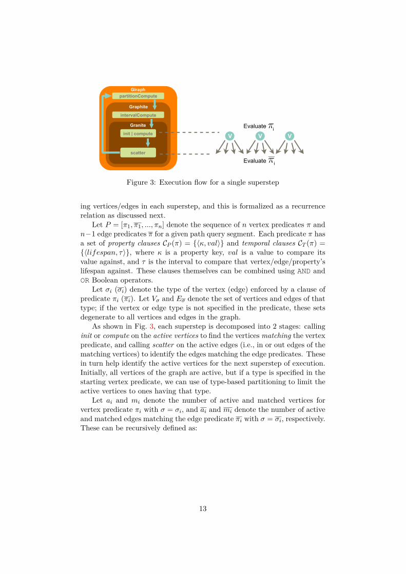
Figure 3: Execution flow for a single superstep

ing vertices/edges in each superstep, and this is formalized as a recurrencerelation as discussed next.

Let P = [π1, π1, ..., πn] denote the sequence of n vertex predicates π andn−1 edge predicates π for a given path query segment. Each predicate π hasa set of property clauses CP (π) = 〈κ, val〉 and temporal clauses CT (π) =〈lifespan, τ〉, where κ is a property key, val is a value to compare itsvalue against, and τ is the interval to compare that vertex/edge/property’slifespan against. These clauses themselves can be combined using AND andOR Boolean operators.

Let σi (σi) denote the type of the vertex (edge) enforced by a clause ofpredicate πi (πi). Let Vσ and Eσ denote the set of vertices and edges of thattype; if the vertex or edge type is not specified in the predicate, these setsdegenerate to all vertices and edges in the graph.

As shown in Fig. 3, each superstep is decomposed into 2 stages: callinginit or compute on the active vertices to find the verticesmatching the vertexpredicate, and calling scatter on the active edges (i.e., in or out edges of thematching vertices) to identify the edges matching the edge predicates. Thesein turn help identify the active vertices for the next superstep of execution.Initially, all vertices of the graph are active, but if a type is specified in thestarting vertex predicate, we can use of type-based partitioning to limit theactive vertices to ones having that type.

Let ai and mi denote the number of active and matched vertices forvertex predicate πi with σ = σi, and ai and mi denote the number of activeand matched edges matching the edge predicate πi with σ = σi, respectively.These can be recursively defined as:

13

ai =|Vσ| , if i = 1min(mi−1, |Vσ|) , otherwise (1)

〈fi, δiin, δiout〉 =⊗

〈κ,val〉∈CP (πi)〈lifespan,τ〉∈CT (πi)

Hκ(val, τ)

mi = ai ×fi|Vσ|

(2)

ai = mσi × (δiin + δiout) (3)

〈fi,−,−〉 =⊗

〈κ,val〉∈CP (πi)〈lifespan,τ〉∈CT (πi)

Hκ(val, τ)

mi = ai ×fi

|Vσ| × (δσin + δσout)(4)

In Eqn. 1, we set the active vertex count in the first superstep to beequal to the number of vertices of type σ. This reflects the localization ofthe search space in the init function to only vertices in the partition matchingthat vertex type. For subsequent supersteps, the active vertex search spaceis upper-bound by |Vσ| but is usually expected to be the number of matchingedges in the previous superstep (in worst case), which would send a messageto activate these vertices and call its compute function.

Next, in Eqn. 2, we use the graph statistics to find the % of vertices thatmatch the vertex predicate πi (right hand term, also called selectivity) andmultiply this with the number of active vertices to estimate the matchedvertices. This is the expected matched output count from init or compute.For the selectivity, we iterate through all clauses of predicate πi, get thefrequency, average in degree and average out degree of the vertex matchesfor each property clause, in conjunction with any temporal clause using H,and aggregate (⊗) these frequencies. The aggregation between adjacentclauses can be either AND or OR, and based on this, we apply the followingaggregation logic for the frequencies and degrees.⊗

(f1, f2) =

min(f1, f2) , if ⊗ = ANDmax(f1, f2) , if ⊗ = OR

(5)

⊗(〈δi, fi〉, ...) =

∑i fi × δi∑i fi

(6)

In Eqn. 5, doing an AND returns the smaller of the frequencies whiledoing an OR gives the larger of the two; the former can be an over-estimatewhile the latter an under-estimate. In Eqn. 6, we get the weighted averageof the degrees of the vertices matching the predicates. Once we have theaggregated frequencies of the clauses, we divide it by the number of verticesof this vertex type to get the selectivity for the vertex predicate.

14

In Eqn. 3, we identify the number of edges for which scatter will betriggered by multiplying the matched vertices with the aggregated in andout degrees for the matching vertices, δ. Lastly, we estimate the number ofedges matched by the edge predicate πi in Eqn. 4. Here, we get the edgeselectivity (right hand term) using the frequency of edge matches returnedby the graph statistics, and normalized by the number of preceding verticesof type σ times the average of the in and out degrees of vertices of this type.The edge selectivity is multiplied by the active edge count to get the matchededges that is expected from the scatter call. These edges will message theirdestination vertices, and this will form the active vertex count in superstepi+ 1.

5.3 Execution Time Estimate

Given the estimates of the active/matched vertices/edges in each superstep,we incorporate them into execution time models for the different stageswithin a superstep to predict the overall execution time. We use micro-benchmarks to develop a linear regression equation for these execution timemodels, I,M,S, CC, and IC as used below. These models are unique to acluster deployment of Granite, and can be reused across graphs and queries.

As shown in Fig. 3, the init function is called on the a1 active vertices inthe first superstep, and generates m1 outputs that affect the internal statesof the interval vertex, and its execution time is given by ι = I(a0,m0). Forsubsequent supersteps i, compute function is called similarly on the activevertices ai to generate matched verticesmi. This has a slightly different exe-cution model since it has to process an estimated mi−1 input messages fromthe previous superstep and does not have to do data structure initializationslike init. It takes time ci = M(ai,mi,mi−1). In a superstep i, scatter iscalled on the active edges and generates matched edges, for an estimatedtime of si = S(ai,mi).

Besides these, there are two per-superstep overheads of the platform: forselecting the vertices matching a given type, cci = CC(|Vσ|), and a per activevertex overhead of Graphite, ici = IC(ai).

Given these, the total estimated execution time of the cost model for apath segment with n hops is

T = (ι+ s1 + cc1 + ic1) +n∑2ci + si + cci + ici

15

PersonLifespan: Integer IntervallastName: Stringgender: Stringbirthday: Datecountry: StringhasInterest: List<String>studyAt: StringworksAt: String

person_knows_personLifespan : Integer Interval

PostLifespan: Integer Intervallength: 32-bit Integercountry: StringhasTag: List<String>

CommentLifespan : Integer Intervallength: 32-bit Integercountry: StringhasTag: List<String>

ForumLifespan: Integer intervaltitle: StringhasTag: List<String>

post_hasCreator_personLifespan : Integer Interval

person_likes_postLifespan : Integer Interval0..*

1 0..*

0..*

comment_hasCreator_personLifespan : Integer Interval

person_likes_commentLifespan : Integer Interval

0..*

0..*0..*

1

comment_replyOf_postLifespan : Integer Interval

comment_replyOf_commentLifespan : Integer Interval

0..*

0..*

1

1

forum_hasModerator_personLifespan : Integer Interval forum_hasMember_person

Lifespan: Integer Interval 0..* 0..*

1 1..*

forum_containerOf_postLifespan : Integer Interval

11..*

0..*

0..*

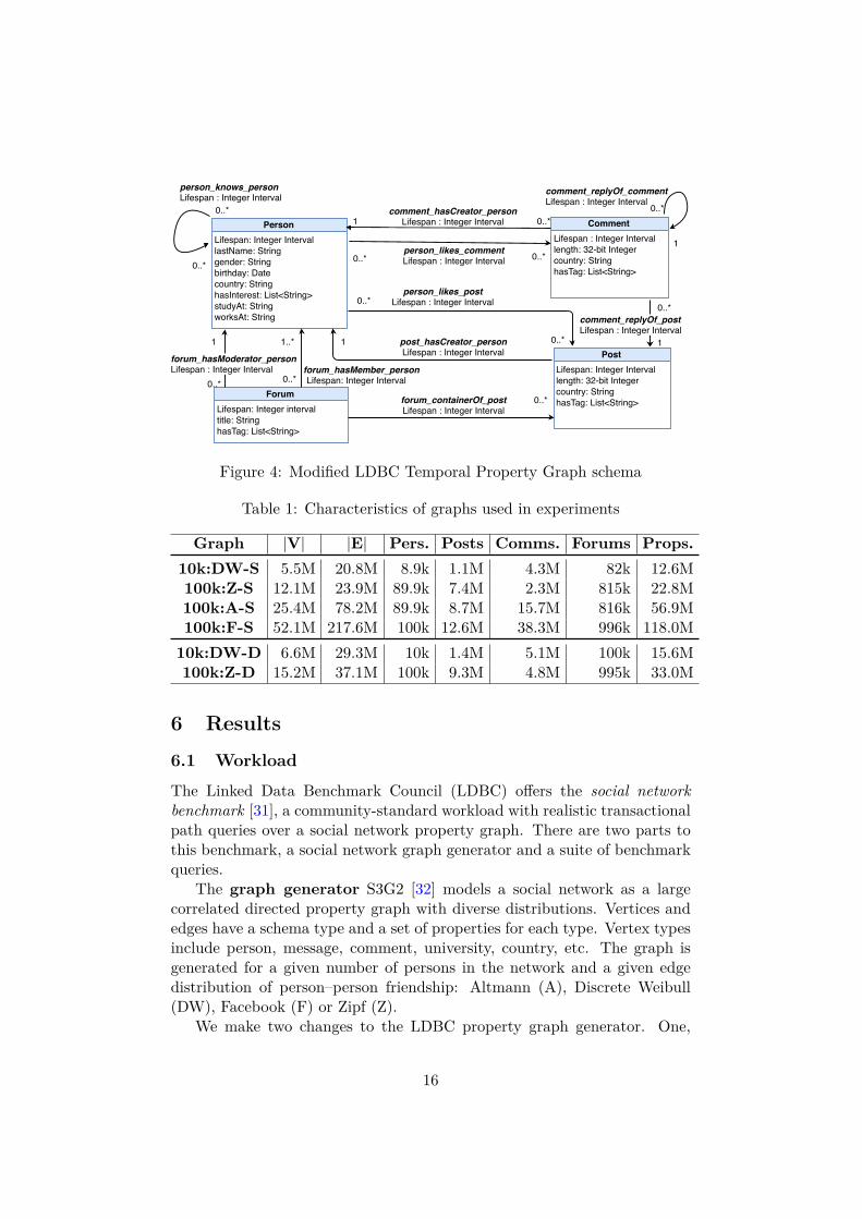
Figure 4: Modified LDBC Temporal Property Graph schema

Table 1: Characteristics of graphs used in experiments

Graph |V| |E| Pers. Posts Comms. Forums Props.10k:DW-S 5.5M 20.8M 8.9k 1.1M 4.3M 82k 12.6M100k:Z-S 12.1M 23.9M 89.9k 7.4M 2.3M 815k 22.8M100k:A-S 25.4M 78.2M 89.9k 8.7M 15.7M 816k 56.9M100k:F-S 52.1M 217.6M 100k 12.6M 38.3M 996k 118.0M10k:DW-D 6.6M 29.3M 10k 1.4M 5.1M 100k 15.6M100k:Z-D 15.2M 37.1M 100k 9.3M 4.8M 995k 33.0M

6 Results

6.1 Workload

The Linked Data Benchmark Council (LDBC) offers the social networkbenchmark [31], a community-standard workload with realistic transactionalpath queries over a social network property graph. There are two parts tothis benchmark, a social network graph generator and a suite of benchmarkqueries.

The graph generator S3G2 [32] models a social network as a largecorrelated directed property graph with diverse distributions. Vertices andedges have a schema type and a set of properties for each type. Vertex typesinclude person, message, comment, university, country, etc. The graph isgenerated for a given number of persons in the network and a given edgedistribution of person–person friendship: Altmann (A), Discrete Weibull(DW), Facebook (F) or Zipf (Z).

We make two changes to the LDBC property graph generator. One,

16

Table 2: Specification of our query workload

Query LDBC ID Hops Prop. Preds. Time Preds. ER Pred.?Q1 BI/Q9 3 4 1 YesQ2 BI/Q10 2 6 1 NoQ3 BI/Q16 3 6 1 YesQ4 BI/Q17 4 3 2 YesQ5 – 5 7 3 YesQ6 – 5 7 1 YesQ7 BI/Q23 4 5 3 YesQ8 IW/Q11 3 3 1 Yes

we denormalize the schema to embed some vertex types such as country,company, university and tag as properties inside person, forum, post andcomment vertices. This simplifies the data model. Two, while LDBC verticeshave a creation time that can span a 3-year period, we include an end time of∞ to form an interval. We assign lifespans to the edges incident on verticesbased on their referential integrity constraints and properties like join date,post date, etc. The vertex and edge lifespans are also inherited by theirproperties. Fig. 4 shows the modified graph schema.

However, this is still only a static temporal property graph. To addressthis, we introduce temporal variability into the properties, worksAt, countryand hasInterest of the Person vertex. For worksAt, we generate a new prop-erty every year using the LDBC distribution; the country is correlated withworksAt, and hence updated as well. We update the hasInterest propertybased on the list of tags for a forum that a person joins, at different timepoints.

Table 1 shows the vertex and edge counts, the number of vertices of eachtype and the total number of properties, for graphs we generate with 103

(10k) or 104 (100k) persons, different distributions (DW, Z, A, F), and withstatic (S, top 4 rows) and dynamic (D, bottom 2 rows) properties.

We select a subset of query templates provided in the LDBC queryworkload [31] that conform to a linear path query, and adapt them for ourtemporal graphs. These are either from the business intelligence (BI) or theinteractive workload (IW). We also include two additional query templatesto exercise our query model. Table 2 and 3 summarizes the query templates.Each template has some parameterized property or time value. We generate100 query instances for each template by randomly selecting a value for theparameters, evaluating the query on the temporal graph, and ensuring thatthere is at least 1 valid result set in most cases. This reflects the expressivityof our query model, and ability to intuitively extend it to the time domain.

In our experiments, each query is given an execution budget of 600 secs,after which it is terminated and marked as failed.

17

Table 3: Description of our query workload

Query Description of path to find (Parameterized property val-ues are underlined)

Q1 Two messages with different tags belong to the same forum,with a time ordering between the messages

Q2 A person with a given tag creates a message with the sametag after a given date.

Q3 A person from a given country has commented or liked apost before a person from another given country.

Q4 Mutual friendships between three persons, but with a time-respecting order in which they befriend each other.

Q5 A person posts a message with a given tag to a forum and,after a time offset, they post another message to the sameforum with a different tag.

Q6 A person with a specific gender replies to a post after anotherperson replies to it.

Q7 A person posts a message from outside their home country,then befriends another person, and that person then postsanother message from outside their home country.

Q8 Two persons working in different companies have a commonfriend at a timepoint.

6.2 Experiment Setup

Our commodity cluster has nodes with one Intel Xeon E5-2620 v4 CPU with8 cores (16 HT) @ 2.10GHz, 64 GB RAM and 1 Gbps Ethernet, runningCentOS v7. For some shared-memory experiments for other baseline graphplatforms, we also use a “big memory” machine with 2 similar CPUs and512 GB RAM. Granite is implemented over our in-house Graphite v1.0,Apache Giraph v1.3.0, Hadoop v3.1.1 and Java v1.8. By default, our dis-tributed experiments use 8 nodes in this cluster, run one Granite workerJVM per machine with 8 threads per worker and 50 GB RAM availableto the JVM. The graphs are initially loaded into Granite from JSON filesstored in HDFS, along with their cost model statistics.

6.3 Baseline Graph Platforms

We use the widely-used Neo4J Community Edition v3.2.3 as a baseline.This is a single-machine, single-threaded graph database. We have threevariants of this. One specifies the workload queries using the Gremlin querylanguage (N4J-Gr, in our plots), a community standard, and the other usesNeo4J’s native Cypher language (N4J-Cy). Both these variants run on asingle node with 50 GB heap size. A third variant uses Cypher as well, but

18

1 2 3 4 CMFixed split point vs. Cost Model

0

100

200

300

400

500

600

700

800

% o

ver O

ptim

al

178.0

1.3 0.0

278.2

0.0

(a) Distribution of queries that exceed theoptimal plan’s time by a % (Y axis) for eachfixed plan and the cost model, for 100k:A-Sgraph on Q4 type queries

10k_DW:S100k_Z:S

100k_A:S100k_F:S

10k_DW:D100k_Z:D

0

20

40

60

80

100

% o

f Que

ries

Optimal 2nd Best Rest

(b) Cost Model Accuracy, all graphs

Figure 5: Effectiveness of cost model in picking the best plan

is allocated 8 × 50 = 400 GB of RAM on the big memory machine (N4J-Cy-M ). This matches the total memory available to our distributed setup.As graph platforms are memory bound, this assigns it equal memory as thedistributed platforms. We build indexes on all properties.

There are few open source distributed graph engines available. Janus-Graph, a fork from Titan, is popular, and uses Apache Spark v2.4.0 as adistributed backend engine to run Gremlin queries (Spark, in our plots). Ituses Apache Cassandra v2.2.10 to store and access the input graph. Sparkruns on 8 compute nodes with 1 worker each and 50 GB heap memory perworker. Cassandra is deployed on 8 other nodes. For all baselines, we followthe standard performance tuning guidelines provided in their documenta-tion.

Since these platforms do not easily support temporal queries over dy-namic temporal graphs, we transform the graphs into a static temporalgraph [25] that allows us to adapt the query to operate over, although overa much bloated graph.

6.4 Effectiveness of Cost Model

We first evaluate the effectiveness of Granite’s cost model in identifying theoptimal split point for the distributed query execution. For each query type,we execute its 100 queries and all their query plans. From the execution timeof all plans for a query, we pick the smallest as its optimal plan. We thencompare this against the plan selected by our cost model, and report the

19

Table 4: % excess time spent over Optimal plan by the Cost Model selectedplan, for different query percentiles

(a)10

0k:A

-S Per’tile Q1 Q2 Q3 Q4 Q5 Q6 Q775 1.8 0 2.2 0 0 0 090 6.8 0 12.6 0 0 0 095 8.5 0 24.6 0 56 0 099 17.6 0 47.1 0 123 0 195

(b)10

0k:Z-D Per’tile Q1 Q2 Q3 Q4 Q5 Q6 Q7 Q8

75 0 0 36 0 0 0 0 090 2 0 101 0 1.9 0 0 5595 30 0 169 0 5.4 0 0 13599 50 0 365 165 38.7 0 188 187

% of excess execution time that the plan selected by our cost model takesabove the optimal plan. This is the effective time penalty when we select asub-optimal plan.

Fig. 5a shows a violin plot of the the distribution of the % excess timeover optimal for the different fixed split points executed for the 100 queriesof type Q4 on graph 100k:A-S. We also report the distribution for the planselected by our cost model. This illustrates that the execution time varieswidely across the plans, with some taking 8× longer than optimal. We alsoobserve that some split points like 2 and 3 are in general better than theothers, but among them, neither are consistently better. This is seen bythe lower median of 2.9% excess time taken by the cost model, compare to12.2% and 6.9% by these other split points. Also, it is not possible to apriori find a single fixed split point which is generally better than the rest,without running the queries using all split points. These motivate the needfor an automated analytical cost model for query plan selection.

Table 4 shows for different query types (columns), and for different per-centiles of their queries (rows), what is the % excess execution time over theoptimal spent by the plan chosen by the cost model. This is reported onlyfor 100k:A-S (top) and 100k:Z-D (bottom) graphs for brevity.

For 100k:A-S, the selected plan are within 2% of optimal execution timefor the 75th percentile query within a query type, and within 13% for 90thpercentile query. Its only at the 95th percentile that we see higher penaltiesof 8–56% for 3 of the 7 types. Even for the dynamic graph 100k:Z-D, at the90th percentile query, 6 of the 8 query types have negligible time penalties,and two have higher penalties of 55–101%. This means we pre-dominantlypick a plan that is optimal, or has an execution time close to the optimalplan.

This is further evident in Fig. 5b which reports that across all queriesand graphs evaluated, our cost model picks the best (optimal) or the second

20

Q1 Q2 Q3 Q4 Q5 Q6 Q7Query Type

101

103

105

107Av

g. E

xec.

Tim

e (m

s) N4J-CyN4J-Gr

GraniteSpark

N4J-Cy-M

(a) 10k:DW-S

Q1 Q2 Q3 Q4 Q5 Q6 Q7Query Type

101

103

105

107

Avg.

Exe

c. T

ime

(ms) N4J-Cy

N4J-GrGraniteSpark

N4J-Cy-M

(b) 100k:Z-S

Q1 Q2 Q3 Q4 Q5 Q6 Q7Query Type

101

103

105

107

Avg.

Exe

c. T

ime

(ms)

DNF

DNR

DNR

DNR

DNR

DNR

DNR

DNR

N4J-CyN4J-Gr

GraniteSpark

N4J-Cy-M

(c) 100k:A-S

Q1 Q2 Q3 Q4 Q5 Q6 Q7Query Type

101

103

105

107

Avg.

Exe

c. T

ime

(ms)

DNF

DNF

DNF

DNF

DNF

DNF

DNF

DNF

DNR

DNR

DNR

DNR

DNR

DNR

DNR

N4J-CyN4J-Gr

GraniteSpark

N4J-Cy-M

(d) 100k:F-S

Figure 6: Comparison of Granite with baseline systems, for static temporalgraphs

best plan over 95% of the time. So while our cost model is not perfect, itsaccuracy is high enough to discriminate between the better and the worseplans.

6.5 Comparison with Baselines

Figs. 6a–6d show the average execution time (log scale) for the query work-load on Granite and the baseline platforms for the static temporal graphs,and Figs. 7a and 7b for the dynamic temporal graphs. Only queries thatcomplete in the 600 sec time budget are plotted. As Table 5 shows, Janus-Spark did not run (DNR) for several larger graphs due to resource limitswhen loading the graph in-memory from Cassandra. 50–85% of queries didnot finish (DNF) on Neo4J for 100k:F-S, the largest graph. Granite com-pletes all queries on all graphs, often within 1sec. For the largest graph100k:F-S, we only run 10 queries per type for all platforms due to timelimits, and Granite uses 16 nodes to fit the graph in distributed memory.

The bar plots show that Granite is much faster than the baselines, across

21

Q1 Q2 Q3 Q4 Q5 Q6 Q7 Q8Query Type

101

103

105

107Av

g. E

xec.

Tim

e (m

s)

DNR

DNR

DNR

DNR

DNR

DNR

DNR

DNR

N4J-CyN4J-Gr

GraniteSpark

N4J-Cy-M

(a) 10k:DW-D

Q1 Q2 Q3 Q4 Q5 Q6 Q7 Q8Query Type

101

103

105

107

Avg.

Exe

c. T

ime

(ms)

DNR

DNR

DNR

DNR

DNR

DNR

DNR

DNR

N4J-CyN4J-Gr

GraniteSpark

N4J-Cy-M

(b) 100k:Z-D

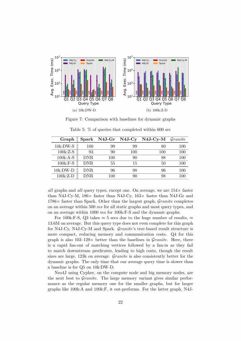
Figure 7: Comparison with baselines for dynamic graphs

Table 5: % of queries that completed within 600 sec

Graph Spark N4J-Gr N4J-Cy N4J-Cy-M Granite10k:DW-S 100 99 99 80 100100k:Z-S 93 90 100 100 100100k:A-S DNR 100 90 98 100100k:F-S DNR 55 15 50 100

10k:DW-D DNR 96 98 96 100100k:Z-D DNR 100 90 98 100

all graphs and all query types, except one. On average, we are 154× fasterthan N4J-Cy-M, 186× faster than N4J-Cy, 163× faster than N4J-Gr and1786× faster than Spark. Other than the largest graph, Granite completeson an average within 500 ms for all static graphs and most query types, andon an average within 1000 ms for 100k:F-S and the dynamic graphs.

For 100k:F-S, Q3 takes ≈ 5 secs due to the huge number of results, ≈13.6M on average. But this query type does not even complete for this graphfor N4J-Cy, N4J-Cy-M and Spark. Granite’s tree-based result structure ismore compact, reducing memory and communication costs. Q4 for thisgraph is also 103–129× better than the baselines in Granite. Here, thereis a rapid fan-out of matching vertices followed by a fan-in as they failto match downstream predicates, leading to high costs, though the resultsizes are large, 123k on average. Granite is also consistently better for thedynamic graphs. The only time that our average query time is slower thana baseline is for Q5 on 10k:DW-D.

Neo4J using Cypher, on the compute node and big memory nodes, arethe next best to Granite. The large memory variant gives similar perfor-mance as the regular memory one for the smaller graphs, but for largergraphs like 100k:A and 100k:F, it out-performs. For the latter graph, N4J-

22

Cy could not finish several query types. Though Neo4J uses indexes to helpfilter the vertices for the first hop, query processing for later hops involves abreadth first search traversal and pruning of paths based on the predicates.There are also complex joins between consecutive edges along the path toapply the temporal edge relation. These affect their times. The executiontimes for Gremlin and Cypher variants of Neo4J are comparable, with nostrong performance skew either way. Interestingly, the Gremlin variant ofNeo4J is able to run most query workloads for all graph, albeit with slowerperformance.

The JanusGraph-Spark distributed baseline takes the highest amount oftime for all these queries. There is a static overhead in Spark in dynamicallyfetching the graph from Cassandra during query execution time, causing an≈ 80 secs overhead to each query. Granite persists the graph in-memoryacross queries. Despite using distributed machines, Spark is unable to loadlarge graphs in memory and often fails to complete execution within thetime budget. A similar challenge was seen even for alternative engines like,Hadoop, used by JanusGraph and Spark was the best of the lot.

In the bar plots, we also show a black bar for the single-machine base-lines, which is the 1/8th execution timepoint – this shows the theoretical timethat would be taken by these platforms with perfect scaling on 8 machines,though it is not supported. As we see, Granite is often able to complete itsexecution within that mark, showing that our distributed engine shows scal-ing performance comparable or better than highly optimized single-machineplatforms.

7 ConclusionsIn this paper, we have motivated the need for and gap in querying over tem-poral property graphs. We have proposed an intuitive temporal path querymodel to express a wide variety of requirements over such graphs, and de-signed the Granite distributed engine to implement these at scale over theGraphite ICM platform. Our novel analytical cost model uses concise in-formation about the graph to give highly accurate selection of alternativedistributed query execution plans. These are validated through rigorousexperiments over 5 graphs and 800 queries derived from the LDBC bench-mark, and Granite uniformly out-performs the baseline graph databases anddistributed platforms.

As future work, we plan to explore out of core execution models to scalebeyond distributed memory, indexing techniques to accelerate performance,and more generalized temporal tree and reachability query models.

23

AcknowledgmentsWe thank Ravishankar Joshi from BITS-Pilani, Goa for his assistance withthe experiments, and Swapnil Gandhi for his assistance with using and ex-tending the Graphite platform. We thank the members of the DREAM:Labfor their help with reviewing and offering feedback on the paper.Shriram Ramesh was supported by the Maersk CDS M.Tech. Fellowship.Yogesh Simmhan was supported by the SwarnaJayanti Fellowship.

References[1] T. Mitchell et al., “Never-ending learning,” Communications of the

ACM, 2018.

[2] M. Cha, H. Haddadi, F. Benevenuto, and K. P. Gummadi, “Measuringuser influence in twitter: The million follower fallacy,” in AAAI weblogsand social media, 2010.

[3] B. Haslhofer, R. Karl, and E. Filtz, “O bitcoin where art thou? insightinto large-scale transaction graphs.”

[4] K. Shu, A. Sliva, S. Wang, J. Tang, and H. Liu, “Fake news detection onsocial media: A data mining perspective,” ACM SIGKDD ExplorationsNewsletter, 2017.

[5] W. Fan, “Graph pattern matching revised for social network analysis,”in ICDT, ser. ICDT ’12. ACM, 2012.

[6] Sharp, Austin et al., “Janusgraph.” [Online]. Available: https://janusgraph.org/

[7] Y. Guo et al., “How well do graph-processing platforms perform? anempirical performance evaluation and analysis,” in IPDPS. IEEE,2014.

[8] G. Malewicz et al., “Pregel: a system for large-scale graph processing,”in SIGMOD. ACM, 2010.

[9] Y. Simmhan et al., “Goffish: A sub-graph centric framework for large-scale graph analytics,” in ECPP. Springer, 2014.

[10] J. E. Gonzalez, R. S. Xin, A. Dave, D. Crankshaw, M. J. Franklin,and I. Stoica, “Graphx: Graph processing in a distributed dataflowframework,” in USENIX (OSDI 14), 2014.

[11] H. Chen, M. Liu, Y. Zhao, X. Yan, D. Yan, and J. Cheng, “G-miner:An efficient task-oriented graph mining system,” in EuroSys, 2018.

24

[12] D. Gregor and A. Lumsdaine, “The parallel bgl: A generic library fordistributed graph computations,” POOSC, 2005.

[13] H.-V. Dang et al., “A lightweight communication runtime for dis-tributed graph analytics,” in IPDPS. IEEE, 2018.

[14] Y. Simmhan et al., “Distributed programming over time-series graphs,”in IPDPS. IEEE, 2015.

[15] W. Han et al., “Chronos: a graph engine for temporal graph analysis,”in EuroSys. ACM, 2014.

[16] S. Gandhi and Y. Simmhan, “An interval-centric model for distributedcomputing over temporal graphs,” in To appear in ICDE. IEEE, 2020.

[17] T. A. Zakian, L. A. Capelli, and Z. Hu, “Incrementalization of vertex-centric programs,” in IPDPS. IEEE, 2019.

[18] R. Cheng et al., “Kineograph: taking the pulse of a fast-changing andconnected world,” in EuroSys. ACM, 2012.

[19] D. Chavarría-Miranda, V. G. Castellana, A. Morari, D. Haglin, andJ. Feo, “Graql: A query language for high-performance attributed graphdatabases,” in IPDPS Workshops. IEEE, 2016.

[20] J. Zhou, G. V. Bochmann, and Z. Shi, “Distributed query processingin an ad-hoc semantic web data sharing system,” in IPDPS Workshops.IEEE, 2013.

[21] N. Jamadagni and Y. Simmhan, “Godb: From batch processing todistributed querying over property graphs,” in CCGrid. IEEE, 2016.

[22] M. Sarwat, S. Elnikety, Y. He, and M. F. Mokbel, “Horton+: A dis-tributed system for processing declarative reachability queries over par-titioned graphs,” Proc. VLDB Endow.

[23] K. Semertzidis and E. Pitoura, “Top-k durable graph pattern querieson temporal graphs,” IEEE TKDE, 2018.

[24] K. Semertzidis, E. Pitoura, and K. Lillis, “Timereach: Historical reach-ability queries on evolving graphs.” in EDBT, 2015.

[25] H. Wu, Y. Huang, J. Cheng, J. Li, and Y. Ke, “Reachability and time-based path queries in temporal graphs,” in ICDE. IEEE, 2016.

[26] J. Byun, S. Woo, and D. Kim, “Chronograph: Enabling temporal graphtraversals for efficient information diffusion analysis over time,” IEEETKDE, 2019.

25

[27] J. Allen, “Maintaining knowledge about temporal intervals,” 1983.

[28] V. Z. Moffitt and J. Stoyanovich, “Temporal graph algebra,” in ISDPL.ACM, 2017.

[29] G. Karypis and V. Kumar, “A fast and high quality multilevel schemefor partitioning irregular graphs,” SIAM Journal on scientific Comput-ing, 1998.

[30] S. Muthukrishnan, V. Poosala, and T. Suel, “On rectangular partition-ings in two dimensions: Algorithms, complexity and applications,” inICDT. Springer, 1999.

[31] “The ldbc social network benchmark (version 0.3.2),” Linked DataBenchmark Council, Tech. Rep., 2019.

[32] M.-D. Pham, P. Boncz, and O. Erling, “S3g2: A scalable structure-correlated social graph generator,” in Selected Topics in Perfor-mance Evaluation and Benchmarking, R. Nambiar and M. Poess, Eds.Springer Berlin Heidelberg, 2013.

26