*lssts1013@hust.edu.cn (Shi Tao)

1

A distribution function correction-based immersed boundary-

lattice Boltzmann method with truly second-order accuracy for

fluid-solid flows

Shi Tao*, Qing He, Baiman Chen, Simin Huang

Key Laboratory of Distributed Energy Systems of Guangdong Province, Dongguan University of Technology,

Dongguan 523808, China

Abstract

The immersed boundary lattice Boltzmann method (IB-LBM) has been widely used in the simulation

of fluid-solid interaction and particulate flow problems, since proposed in 2004. However, it is usually a

non-trivial task to retain the flexibility and the accuracy simultaneously in the implementation of this

approach. Based on the intrinsic nature of the LBM, we propose a simple and second-order accurate IB-

LBM in this paper, where the no-slip boundary condition on the fluid-solid interface is directly imposed

by iteratively correcting the distribution function near the boundary, markedly similar to the treatment of

boundary condition in the original LBM. Therefore, there are no additional efforts needed to construct

an interfacial force model (such as the spring, feedback and direct force models) and absorb this force

into the framework of LBM. It is worth mentioning that we retain the discrete delta function for the

connection between the Lagrangian and Eulerian meshes, thus preserving the flexibility of the

conventional IB-LBM. Second-order accuracy of the present IB-LBM is reasonably confirmed in the

simulation of cylindrical Couette flow, while the conventional approach is generally a first-order scheme.

The present method is first validated in the flow past a fixed cylinder. No streamline penetration is found,

indicating the exactly enforcement of the no-slip boundary condition. Furthermore, in the simulations of

one and two particles settling under gravity, good agreements can be observed comparing with the data

available in the literature.

Keywords: Lattice Boltzmann method; immersed boundary scheme; second-order accuracy; distribution

function correction; fluid-particle flows

1. Introduction

The immersed boundary method (IBM) is a very popular numerical approach in the simulation of

complex and moving boundary problems [1–3]. Since it is generally based on the fixed Cartesien grids,

the time-consuming procedure for mesh-generation and remeshing involved in other methods, such as

the Arbitrary-Lagrange-Euler (ALE) that uses a body-fitted grid and regenerates the computation mesh

whenever the boundary moves, can be totally removed. The IBM is usually applied to handle the

boundary of a body. Therefore, an efficient flow solver is needed to simulate the flow of the carrier fluid.

In most cases in the past, IBM was combined with the Navier-Stokes (N-S) solvers. Recently, some

efforts were also made to combine IBM with the lattice Boltzmann method (LBM) [4–6]. Compared to

the traditional N-S solvers, a noteworthy feature of LBM is that it is a kinetic scheme. Hence, there is no

2

need for LBM to solve the time-consuming Poisson equation, since the pressure in LBM is determined

directly by the equation of state. In addition, the LBM has some other distinctive merits, such as easy

implementation and natural parallelism. For those reasons, the application of LBM as an alternative flow

solver has been advanced dramatically in recent years [7,8]. A pioneering work from Feng et al. [4] first

successfully combined the IBM with LBM in 2004, considering that the LBM is also based on the

uniform Cartesien grids. This hybrid approach, named IB-LBM, has then been demonstrated to well

preserve the mutual advantages of the individual methods, and more and more widely used to deal with

the fluid-solid interaction and particulate flow problems [9–12,66].

In IBM, the solid boundary is usually modeled as a generator of external force. This force will be

added into the governing equation of fluid, and can then affect the macroscopic quantities. So that the

no-slip boundary condition on the surface of immersed body is to be imposed. The IBM generally falls

into two categories: the continuous forcing and discrete forcing methods [13]. The discrete forcing

method is a sharp interface scheme, where the external body force is applied unilaterally around the

boundary or contained implicitly in the discrete governing equation. Even though the discrete forcing

approach has high accuracy for the boundary treatment, a major disadvantage is that serious spurious-

force-oscillation (SFO) is almost inevitably to emerge when the boundary moves [14-16]. It is still a

challenging and ongoing subject for researchers to remove such deficiency. Furthermore, the original

LBM itself is a sharp interface scheme (the bounce-back type methods used in the boundary treatment),

and hence experiences the same problem of SFO when applied it to moving boundaries [17,18,61].

Together with the complex algorithm for application in the discrete forcing method, all those result in

that it is not so attractive to combine that scheme with LBM. On the other hand, continuous forcing is a

diffuse interface scheme, where the solid interface smears in several grids at both sides of the boundary.

The bilateral fluid is treated in the same manner, which drastically reduces the difficulty in applications.

An accompanying advantage is that the phenomenon of SFO can be well removed in the continuous

forcing method. In general, the focus of the recent studies seems to be more on the development of

continuous forcing IB-LBM [10,11,19,20] (the term continuous forcing is omitted hereinafter when

referring to IB-LBM).

A tricky problem presently experienced by the IB-LBM is the low precision (usually only first-order

accuracy) for the boundary treatment. Some authors considered it may be caused by the streamline

penetration, a phenomenon first observed by Shu et al. [21] in the simulation of flow past a fixed circular

cylinder. This drawback is subsequently resolved by Wu et al. [5], using a velocity correction- based

implicit forcing technology. Note that the multi-forcing strategy can also be used to efficiently remedy

the deficiency of streamline penetration [22,20]. Furthermore, it has been founded that those above-

mentioned boundary condition-enforced IB-LBMs [5,22] appear to be second-order schemes, all in the

accuracy test through the simulation of Taylor-Green decaying vortices. However, some recent works

reveal that the decaying vortices problem cannot serve as a reliable test case [23,24]. The reason is that

analytical solution is artificially specified at the solid boundary, resulting in a continuous partial

derivative across the interface which is too much idealistic for real applications [24]. In fact, it is usually

not analytically tractable for Taylor-Green decaying vortices flow containing a physical solid boundary.

Therefore, the decaying vortices should be substituted with other reasonable cases, such as the cylindrical

Couette flow and the flow past a cylinder, in the accuracy test. In such situations, the IB-LBMs all

degrade to be first-order accurate [6,23,53]. Many efforts are being devoted to improving the accuracy

of IB-LBM. Most recently, Zhou et al. [25] reported a high-order Runge-Kutta based IB-LBM in 2014,

which was claimed to improve the IB-LBM to be second-order accurate for the first time. The authors

3

adopted the flow past a fixed/moving sphere in a tube as the accuracy test case (it is absolutely reliable),

and a retraction distance (the solid boundary steps a little bit back to the geometry center) was used to

improve the accuracy. They presented an optimal value of such distance for a sphere, i.e., 0.30 times of

the spatial step. However, it is this retraction distance which helps to promote the accuracy of IB-LBM,

because beyond a certain range, the proposed IB-LBM rapidly deteriorates to first-order accuracy. Since

it is an open question to determine an optimal range of retraction distance applicable for different shapes

of body, different discrete delta function and different flow configurations [63,64], there is still a need to

develop a more general second-order accurate IB-LBM.

Other difficulty in the implementation of the conventional IB-LBM is to evaluate and incorporate a

suitable external force within the framework of LBM. First, we should construct an external force model

to compute the force. With the development of IBM, several force models have been proposed, including

the spring force [26], feedback force [27], direct force [28] and momentum exchange force [29]. Note

that the momentum exchange force scheme is a heuristic model derived directly from the bounce-back

rule in the LBM, but has been demonstrated recently to be essentially a direct force model [6]. Those

force models [26-29] have their own advantages and disadvantages, for example, the spring and feedback

models are still stuck with the stiffness problem which requires a very small time step in computations

[13]. Secondly, if the external force at the boundary has been evaluated and distributed to the ambient

fluid (such distribution is usually accomplished with the help of discrete delta function), we should then

determine the influence of this force in the framework of LBM because it is a kinetic method. There are

many schemes for force-absorbing available in the literature. Guo et al. [8,30] systematically compared

the performances of ten such methods. Cheng et al. [31] proposed another force-absorbing approach to

incorporate the non-uniform and unsteady body force. Recently, Zheng et al. [32] presented a kinetic

based force treatment. Note that the force-absorbing schemes should be corrected to adapt to different

LBM models [33–35]. Furthermore, if the non-thermal and/or multi-phase flows encountered, it is still

an open question to choose an appropriate force treatment in LBM [36–38].

Considering the difficulty and drawback outlined above for the conventional IB-LBM, in this work, a

truly second-order IB-LBM for fluid-solid interactions and particulate flows is proposed. The present

method improves the accuracy and preserves the flexibility concurrently of the traditional IB-LBM.

Furthermore, it is based on the intrinsic nature of the LBM, i.e., directly correcting the distribution

functions near the boundary to realize the no-slip boundary condition. Hence, there is no need for force

evaluation and transformation in the present method. The remaining part of this paper is organized as

follows. A methodology introduction is provided in Section 2. The numerical model is validated in

Section 3. Finally, conclusions are summarized in Section 4.

2. Numerical methodology

The distribution function correction-based immersed boundary-lattice Boltzmann method is a

combination of the IBM and LBM, for handling the boundary condition and the fluid flow, respectively.

The LBM will be introduced briefly in this section, followed by the details of the immersed boundary

scheme and the present improvements.

2.1. Lattice Boltzmann method

The lattice Boltzmann method is derived from the lattice gas automate (LGA), and has been greatly

advanced to be an alternative incompressible flow solver in recent years [8,40]. As a kinetic scheme, a

4

set of velocity distribution functions 𝑓𝑖(𝒙, 𝑡) at position x, time t and discrete velocity ei, rather than the

macroscopic quantities are tracked in LBM, which are subject to the lattice Boltzmann equation as

, , , 0,1, ..., 1,i i t t i if t f t f i b x e x (1)

where 𝛺𝑖(𝑓) denotes the discrete collision operator, δt the temporal step and b the total number of

discrete velocities. The MRT (multi-relaxation-time) collision model will be adopted instead of the

widely-used LBGK (lattice Bhatnagar-Gross-Krook) model to avoid the unphysical numerical artifact

and improve the stability, in which the collision term is expressed as [39]

1

1

1

= ,b

eq

i j jijj

f f f

M SM (2)

where M is a b × b transform matrix, and S is a relaxation matrix; 𝑓𝑗𝑒𝑞

is the equilibrium distribution

function which depends on the density ρ, velocity u, and temperature T of the gas and is typically defined

as

2 2

2 4 2

. ( . )1 ,

2 2

j jeq

j j

s s s

fc c c

e u e u u (3)

where ωj is the model-dependent weight coefficient, cs = √𝑅𝑇 (R is the gas constant) the lattice sound

speed. For isothermal flows, cs is set to be c/√3 with c = δx /δt, where δx is the lattice spacing (c = 1 in

this paper).

For simplicity and without loss of generality, the D2Q9 model (two dimensions with nine lattice

velocities, b = 9) is employed for two-dimensional flows in the present study, where the velocity set and

the corresponding weight coefficients are defined as

4 / 9, 0,

1/ 9, 1,2,3,4,

1/ 36, 5,6,7,8.

(0,0),

[cos( 1) / 4,sin( 1) / 4],

2[cos( 1) / 4,sin( 1) / 4],

i i

i

i

i

i i

i i

e (4)

The transform matrix M is given by [39]

1 1 1 1 1 1 1 1 1

-4 -1 -1 -1 -1 2 2 2 2

4 -2 -2 -2 -2 1 1 1 1

0 1 0 -1 0 1 -1 -1 1

0 -2 0 2 0 1 -1 -1 1

0 0 1 0 -1 1 1 -1 -1

0 0 -2 0 2 1 1 -1 -1

0 1 -1 1 -1 0 0 0 0

0 0 0 0 0 1 -1 1 -1

M (5)

and the relaxation matrix is [39]

, , , , , , , , 1/ ,1/ ,1/ ,1/ ,1/ ,1/ ,1/ ,1/ ,1/ .e d q d q s s e d q d q s sdiag s s s s s s s s s diag S (6)

where s and τ are the relaxation rate and relaxation time, and (τρ, τd) and the remaining relaxation times

are for conserved and non-conserved moments, which can take arbitrary values and should be set greater

than 0.5, respectively.

Through Chapman-Enskog expansion, the macroscopic fluid density ρ and velocity u can be derived

respectively as the zeroth and first order moments of fi,

5

8 8

0 1

, .i i i

i i

f f

u e (7)

The fluid pressure is directly obtained by 𝑝 = 𝑐𝑠2𝜌, and the fluid viscosity is related to the relaxation

time τs for the shear moment as

2 0.5 .s s tc (8)

2.2. Conventional immersed boundary scheme

Figure 1. Schematic of the 2D immersed boundary method: (a) traditional scheme; (b) present scheme.

In IB-LBM, the IBM is usually used to impose the no-slip boundary condition at the solid-fluid

interface Γ (immersed in fluid ζ), which is discretized into a set of Lagrangian markers X(s, t), shown in

Fig. 1. The main feature of the IBM is to model this interface as a generator of external body force; the

force will then be distributed to the ambient Eulerian points x, appeared finally as a body force term in

the governing equation [1,2]. In this manner, the no-slip boundary condition is replaced by a localized

force field, and the fluid can sense the existence of the solid boundary. Generally, the implementation

process of the IBM mainly contains the following three steps: evaluate the force, transfer the force and

incorporate this force in the governing equation.

We should first calculate the local force at the Lagrangian point. There are several force schemes

available in the literature. Lai et al. [26] proposed a spring force to mimic the rigid boundary as

0, ( , ) ( , ) ,s t k s t s t G X X (9)

where s is Lagrangian coordinate along the boundary, X0(s, t) denotes the expected position of the

boundary, and k is the coefficient of spring stiffness. In this force model, the Lagrangian points X(s, t)

are connected to their desired locations X0(s, t) with a spring. The positive spring constant k is set to be

sufficiently large. Therefore, the boundary points will be put back to their target positions once a small

deviation emerges. The drawback for this spring force model is that a very small time step is required to

obtain computational stability. Furthermore, it is a non-trivial task to determine a reasonable value of k.

A feedback force model was reported by Saiki et al. [27], in which the boundary force is computed as

0

, ( , ) ( , ) ( , ) ( , ) ,t

s t s t s t dt s t s t G u U u U (10)

(a) Conventional IB-LBM

(b) Present IB-LBM

Lagrangian point X(s, t) Solid-fluid interface Γ

δf f g u

Eulerian point x

Fluid domain ζ

6

where u(s, t) is the fluid velocity and U(s, t) is the real boundary velocity, both at position X(s, t); α and

β are two negative and semi-empirical constants. The determination of α and β is the core problem in this

feedback force model, whose values are somewhat relevant to the temporal step. Taking reasonable

values is to bring the velocity discrepancy between u(s, t) and U(s, t) to approach zero. Otherwise, it

would seriously undermine the stability of the whole algorithm. Considering the limitations in the spring

and feedback force models, Silva et al. [28] proposed a direct force scheme, in which the interfacial force

is calculated without ad hoc constants as

. ,pt

uG u u u (11)

where the discrete form for the temporal term is (U – u)/δt. It can be clearly observed that this force is

directly obtained from the N-S equations, owing solid theoretical basis. Subsequently, that direct force

model is further simplified to be a formulation of velocity deviation as [41]

.t

U uG (12)

Since the force model Eq. (12) has a very succinct form, no empirical parameters and no limitations for

the temporal step, it is widely used in the field of IBM [54,55]. Furthermore, when combining this model

with the LBM, some authors [42] claimed that the value of force should be doubled,

2 .t

U uG (13)

Considering that the no-slip boundary condition is gradually enforced in the IBM [21], Hu et al. [6]

exhibited through rigorous mathematical deducing that the number 2 in Eq. (13) should be replaced by a

relaxation parameter of λ with an optimal range of 2.0–2.5. Recently, Niu et al. [29] made use of the

bounce-back rule in the original LBM to construct a new force model as

8

21

., 2 ,i

i i i ii ii s

f f f fc

e U

G e (14)

where 𝑖 is the reverse direction of i, and fi is obtained from fluid by interpolation. However, it can be

proved from Eq. (7) that this scheme is essentially equivalent to the direct force approach [6].

The force calculated by the above-mentioned models is then distributed to the ambient Eulerian points

(Figure 1). In this step, we should determine the influence range and portion that the interfacial force

imposes on the fluid. Many approaches can serve that propose for extrapolation, such as the radial basis

function (RBF) [43], inverse distance weighted (IDW) scheme [44], and the discrete delta function [45].

The latter is more widely used in IBM, with a formulation of D(x – X) as

2

2

2

1,

11 1 3 , 0.5,

31 , 1, 1

( ) ( ) 5 3 1 3(1 ) , 0.5 1.5,60, 1;

0, 1.5,

11 cos , 2,

4 2( )

0, 2;

x

l lD x x y y

r r

r ra r b r r r r

r

r

rr

c r

r

x X

(15)

where (a), (b) and (c) are respectively the 2-, 3- and 4-point functions, and x = (x, y) and X = (xl, yl). The

present work adopts the 4-point discrete delta function to spread the force to the Eulerian points,

7

,D ds

g G x X (16)

Note that this function is also used for the interpolation of fluid velocity u at the Lagrangian point.

If the force exerted on the fluid points is obtained, finally we should add it in the governing equation

of LBM, that is to say, the Eq. (1) as

8

1 1

1

, , / 2 ,eq

i i t t i j j t iijj

f t f t f f

x e x M SM M I S MF (17)

where Fi is the force term that absorbs the external body force evaluated by the force models described

above. Guo et al. [8,30] generalized ten specific forms of Fi, where two representative respectively are

2

., 1 0.5,i i

i

s

n n orc

g eF (18)

2

2 4

:..

i i si

i i

s s

c

c c

ug e e Ie gF (19)

Note that when using the method in Eq. (19) to incorporate the force into the LBM, the fluid velocity

should be calculated as

8

1

0.5 .i i t

i

f

u e g (20)

Cheng et al. [31] proposed another type of Fi as

1 1/ 2 , , ,

2

3 . 3 . ,

i i i t t i

i i i i i

H t H t

H A B

M I S MF x e x

e u e u e

(21)

where A and B are usually set to be 0 and g, respectively.

2.2.1. Iterative forcing approach

The no-slip boundary condition is only approximately satisfied in the above-described IBM, because

the forward/backward interpolation errors is inevitable to cause the unphysical streamline penetration

[5,6,21]. To correct such deficiency, there are generally two strategies available in the literature: implicit

velocity correction [5] and iterative forcing [22]. Considering that the former scheme might introduce

extra computation loads [46], the idea of iterative forcing approach [22] will be adopted in the present

study (even though actually there is no forcing in the present IB-LBM introduced in Section 2.3). The

iterative forcing algorithm repeats the procedure of (i) velocity interpolation, (ii) obtain the force, and

(iii) distribute the force multiple times, to gradually make the discrepancy of velocity at the Lagrangian

point tend to be zero. It is found that within a finite number of iterations about 10, the residual error of

such deviation will be reasonably small [6,22].

2.3. Distribution function correction-based immersed boundary scheme

As outlined above, there are difficulties existing in the implementation of the conventional IB-LBM,

for instance, the model selections for force calculation and incorporating it into LBM. Furthermore, it is

found in some recent studies that the traditional IB-LBM has only first-order accuracy in space [23,24].

Therefore, it motivates us to develop a second-order scheme with no forcing involved, that is, the

distribution function correction-based IB-LBM.

The distribution function correction-based IB-LBM is derived from the original LBM, where the

8

enforcement of boundary condition is accomplished by correcting the distribution functions at points

near the boundary, as depicted in Fig. 2. In original LBM, the (simple or interpolated) bounce-back rule

is usually adopted for such purpose. The reasonably obtained distribution function can make the no-slip

boundary condition at the interface strictly enforced [61,62,65], since the macroscopic quantities are the

moments of the distribution function, presented in Eq. (7). With those foundations in hand, hence, in the

present IB-LBM, the aim is also to directly update the distribution functions around the boundary, both

inside and outside (Fig. 1); so that if they are interpolated back at the interface, the no-slip boundary

condition can be imposed through Eq. (7). For such propose, we first interpolate the uncorrected

distribution function (𝑓𝑖(𝑠, 𝑡))∗ and its non-equilibrium part (𝑓𝑖𝑛𝑒𝑞

(𝑠, 𝑡))∗ at the Lagrangian point

using the discrete delta function of Eq. (15),

*,

( , ) ( , ) , 0,1,...,8,n n

i if t f t D d i

s x x X x (22a)

*,

( , ) ( , ) ,n n

neq neq

i if t f t D d

s x x X x

(22b)

where 𝑓𝑖𝑛𝑒𝑞

= 𝑓𝑖 − 𝑓𝑖𝑒𝑞

, and the superscript n denotes the number of corrections (multiple corrections is

needed, as explained next). The uncorrected non-equilibrium distribution function is approximated as the

desired one at the boundary,

*,

( , ) ( , ) .n n

neq neq

i if s t f s t (23)

Hence, plus the equilibrium part obtained by the information of the boundary (density ρ and velocity U),

the desired distribution function at the boundary can be determined as

*,

( , ) .n n n nn neq eq neq eq

i i i i if f f f f U (24)

A deviation is inevitable between the desired and interpolated distribution functions,

*,

( , ) .n n n

i i if s t f f (25)

This discrepancy is then distributed to the ambient fluid points by the same discrete delta function,

( , ) ( , ) .n n

i if t f s t D ds

x x X (26)

Finally, the distribution function at the Eulerian point can then be corrected one time,

1

( , ) ( , ) ( , ) ,n n n

i i if t f t f t x x x (27)

Note that the above procedure, i.e., Eqs. (22) to (27) should be applied to all the Lagrangian points. A

problem arises when we interpolate the revised distribution function back at the Lagrangian point, an un-

negligible deviation between the revised and desired distribution functions could still be found, indicating

that the no-slip boundary has not been well enforced according to Eq. (7). The reason is obvious because

the range of the discrete delta function for the Lagrangian points may overlap with each other, as

illustrated in Fig. 1. Therefore, it is insufficient to correct the distribution functions once. Here, inspired

by the iterative forcing approach in the conventional IBM, we repeat the above-described process, i.e.,

obtaining the deviation of distribution function at the Lagrangian point and distributing it back to the

Eulerian grids, Eqs. (22)–(27) multiple times. The residual error of deviation of distribution function is

found to be reasonably small within a finite number of iterations N about 10 (n in Eqs. (22) and (27)

takes 0, 1, … , N–1).

9

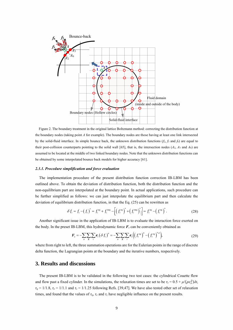
Figure 2. The boundary treatment in the original lattice Boltzmann method: correcting the distribution function at

the boundary nodes (taking point A for example). The boundary nodes are those having at least one link intersected

by the solid-fluid interface. In simple bounce back, the unknown distribution functions (f2, f3 and f6) are equal to

their post-collision counterparts pointing to the solid wall [65], that is, the intersection nodes (A2, A3 and A6) are

assumed to be located at the middle of two linked boundary nodes. Note that the unknown distribution functions can

be obtained by some interpolated bounce back models for higher accuracy [61].

2.3.1. Procedure simplification and force evaluation

The implementation procedure of the present distribution function correction IB-LBM has been

outlined above. To obtain the deviation of distribution function, both the distribution function and the

non-equilibrium part are interpolated at the boundary point. In actual applications, such procedure can

be further simplified as follows: we can just interpolate the equilibrium part and then calculate the

deviation of equilibrium distribution function, in that the Eq. (25) can be rewritten as

* * **

.eq neq eq neq eq eq

i i i i i i i i if f f f f f f f f

(28)

Another significant issue in the application of IB-LBM is to evaluate the interaction force exerted on

the body. In the preset IB-LBM, this hydrodynamic force Fs can be conveniently obtained as

*,

,n nn eq eq

s i i i i i

n i n i

f f f X X

F e e (29)

where from right to left, the three summation operations are for the Eulerian points in the range of discrete

delta function, the Lagrangian points at the boundary and the iterative numbers, respectively.

3. Results and discussions

The present IB-LBM is to be validated in the following two test cases: the cylindrical Couette flow

and flow past a fixed cylinder. In the simulations, the relaxation times are set to be τs = 0.5 + μ/(𝜌𝑐𝑠2)δt,

τq = 1/1.8, τe = 1/1.1 and τε = 1/1.25 following Refs. [39,47]. We have also tested other set of relaxation

times, and found that the values of τq, τe and τε have negligible influence on the present results.

Fluid domain

(inside and outside of the body)

Boundary nodes (Hollow circles)

Solid-fluid interface

f3

f2 f6 Bounce-back

A

A

A6 A2

A3

10

3.1. Accuracy verification

3.1.1. Taylor-Green vortex with a cylinder

The Taylor-Green vortex (TGV) flow containing an artificial circular cylinder is used first to test the

accuracy order of the present IB-LBM. In this flow problem, many versions of IBMs have previously

been considered to be second-order accuracy [5,6]. It is also noted that the reasonability of this flow

taken as the accuracy validation case is questioned very recently [24].

The TGV flow with an artificial circular cylinder is defined in a [－L, L] × [－L, L] square box,

subjected to the analytical solution as

2

2

2

2

0

2

0

2 4

00

cos sin ,

sin cos ,

cos sin .4

tL

x

tL

y

tL

u u x y eL L

u u x y eL L

ux y e

L L

(30)

The diameter of the cylinder is L, embedded in the center of the computation domain. In the simulation,

the Reynolds number of the flow (Re = u0L/ν) is fixed at 10.0, and the relaxation time τs is set to be 0.65,

as the same in Refs. [5,6,33,42]. The initial condition of the flow is obtained by Eq. (30) at t = 0. The

time-dependent boundary conditions at the square and cylinder are given by Eq. (30), implemented by

the non-equilibrium extrapolation scheme [62] and the present IB-LBM, respectively. Four sets of

uniform grids with L = 10, 20, 40 and 80 are used for simulation. At dimensionless time t* = tu0/L = 1,

the numerical solution is obtained and the global error of the velocity field is quantified using the L2-

norm expressed as

2 2

12 norm ,

Nc a c a

x x y y

i

u u u u

LN

(31)

where the superscripts a and c denotes the analytical and numerical solutions, respectively, and N is the

total number of Eulerian points in the flow field.

Velocity magnitude and the streamlines of the flow are presented in Fig. 3(a). Figure 3(b) plots the

global L2-norm error of the velocity, together with the data by the IB-LBM in literature [5,6,33,42] for

comparison. Note that the Kang_1 and Kang_2 imply respectively the results using the 2-point and 4-

point discrete delta functions in Kang et al. [42]. It can be clearly observed that second-order accuracy

for the conventional IB-LBM is generally obtained by the previous works. However, the convergence

rate of the present IB-LBM is almost in third-order for this TGV flow, seemingly in contrary to the

documented conclusion that the original LBM is second-order accurate in space and hence the accuracy

of hybrid scheme (IB-LBM) usually cannot exceed such value. This contradiction may result from the

too much idealization of the TGV flow, since the flow macroscopic quantities and their derivations are

assumed to be smooth at the inner circular interface. Therefore, this interface cannot be considered as the

usual physical solid boundary that more concerned in applications. In general, for this idealized flow

case, the present IB-LBM seems to have advantage over the conventional ones.

Cylinder embedded artificially

11

Figure 3. Contour of velocity magnitude and streamlines in the Taylor-Green vortex flow at δx = 1/80 and t* = 1.

3.1.2. Cylindrical Couette flow

Since the Taylor-Green vortex with an artificial cylinder essentially cannot served as a reasonable test

case of accuracy outlined above, we further explore the accuracy of the present IB-LBM. It has been

well-established that the LBM is a fully second-order scheme [8,40]. After combined with the

conventional IBM, the accuracy reduces to be just first-order, which is found recently [23,24]. Therefore,

it is important to verify the overall accuracy of the present IB-LBM. Note that here we choose the

cylindrical Couette flow, other than the frequently-used decaying Taylor-Green vortex for conducting

the numerical experiment, since the solid boundary exists physically in the former but is added artificially

to the latter case. In the cylindrical Couette flow problem plotted in Fig. 4, the fluid is confined by the

inner and outer rotating cylinders, with speeds ω1, ω2, and radii R1, R2, respectively. This flow is

subjected to the N-S equations using the cylindrical polar coordinate as

2

20,

d u ud

dr rdr

(32)

Coupled with the following boundary conditions (ω2 = 0),

1 2

1 1, 0,r R r R

u R u

(33)

the steady solution of the flow can be obtained as

2 2 2

1 1

2, 0,

1r

R R ru u

R r

(34)

where uθ, ur are the velocity components, r is the radial distance and R = R1/ R2 is the radius ratio.

In the simulations, it is set that the Reynolds number Re = ρU1(R2 – R1)/μ = 10.0 (where U1 = ω1R1),

τs = 0.65, 0.85, and R = 0.5, 0.8. We calculate the L2-norm to evaluate the numerical error as

22

, ,

12 norm

N

x x y r y

i

u u u u

LN

(35)

where ux and uy are the velocity components obtained by the present IB-LBM along the profile θ = π/2

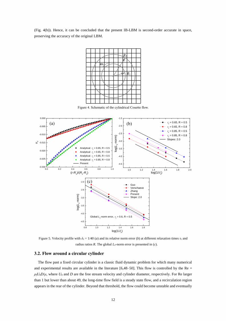
in the cylindrical polar coordinate. The velocity profile with δx = 1/40 and L2-norm error under different

grid resolutions is presented in Fig. 5. The preset results agree well with those of analytical data (Fig.

4(a)). Furthermore, a generally second-order convergence rate can be observed for four sets of τs and R

1.0 1.2 1.4 1.6 1.8 2.0-7

-6

-5

-4

-3

-2

Slope: 2.9

Slope: 1.9

Slope: 3

Slope: 2

log

(L2-n

orm

)

log(1/x)

Wu

Kang_1

Kang_2

Hu

Falagkaris

Present

Slope: 1.98

Slope: 1.986

Slope: 1.99

(a) (b)

12

(Fig. 4(b)). Hence, it can be concluded that the present IB-LBM is second-order accurate in space,

preserving the accuracy of the original LBM.

Figure 4. Schematic of the cylindrical Couette flow.

Figure 5. Velocity profile with δx = 1/40 (a) and its relative norm error (b) at different relaxation times τs and

radius ratios R. The global L2-norm error is presented in (c).

3.2. Flow around a circular cylinder

The flow past a fixed circular cylinder is a classic fluid dynamic problem for which many numerical

and experimental results are available in the literature [6,48–50]. This flow is controlled by the Re =

ρfU0D/μ, where U0 and D are the free stream velocity and cylinder diameter, respectively. For Re larger

than 1 but lower than about 49, the long-time flow field is a steady state flow, and a recirculation region

appears in the rear of the cylinder. Beyond that threshold, the flow could become unstable and eventually

0.0 0.2 0.4 0.6 0.8 1.0-0.030

-0.025

-0.020

-0.015

-0.010

-0.005

0.000

Analytical: s = 0.65, R = 0.5

Analytical: s = 0.65, R = 0.8

Analytical: s = 0.85, R = 0.5

Analytical: s = 0.85, R = 0.8

Present

u

(r-R1)/(R

2-R

1)–

1.0 1.2 1.4 1.6 1.8 2.0

-4.5

-4.0

-3.5

-3.0

-2.5

-2.0

-1.5

lo

g(L

2-n

orm

)

log(1/x)

s = 0.65, R = 0.5

s = 0.65, R = 0.8

s = 0.85, R = 0.5

s = 0.85, R = 0.8

Slopes: 2.0

0.8 1.0 1.2 1.4 1.6 1.8

-4.5

-4.0

-3.5

-3.0

-2.5

-2.0

Global L2-norm error,

s= 0.6, R= 0.5

log

(L2-n

orm

)

log(1/x)

Guo

Verschaeve

Zhang

Present

Slope: 2.0

(a) (b)

ω1

R2

R1

(c)

13

develops the Kármán vortex shedding. The quantitative results of this problem are usually the length of

recirculation zone Lw, separation angle θ, drag force Fd, lift force Fl and frequency of vortex shedding f.

The latter three are respectively defined in the non-dimensional form as

2 2

00 0

, , .0.5 0.5

d l

d l

f f

F F fDC C St

UU D U D (36)

Figure 6. The streamlines around and inside the cylinder at Re = 40.

Table 1. Comparison of the results of flow over a circular cylinder at Re = 20, 40, 100 and 200.

Re 20 40 100 200

Cd Lw/D θ(°) Cd Lw/D θ(°) Cd Cl St Cd Cl St

Russell[48] 2.17 0.93 43.9 1.60 2.29 53.1 1.43 0.322 0.172 1.45 0.63 0.201

Xu[49] 2.23 0.92 44.2 1.66 2.21 53.5 1.423 0.34 0.171 1.42 0.66 0.202

Linnick[50] 2.16 0.93 43.9 1.54 2.28 53.6 1.38 0.337 0.169 1.37 0.7 0.199

Hu[6] 2.213 1.016 — 1.660 2.55 — 1.418 0.367 0.166 1.394 0.712 0.195

Present 2.181 0.987 44.2 1.643 2.46 53.2 1.415 0.358 0.166 1.405 0.719 0.196

In the simulations, size of the computational domain is (40D, 20D), and the circular cylinder is placed

at the coordinate (10D, 10D). A uniform mesh system is adopted, with a grid resolution δx = D/40.

Constant velocity U0 = 0.1 is specified at the inlet, and a free outflow is developed at the outlet. The inlet

and outlet boundary conditions are both implemented by the non-equilibrium extrapolation method [62].

The streamlines near the circular cylinder are depicted in Fig. 6 for Re = 40, even though the inner fluid

is fictitious in physics. It is clearly exhibited that no unphysical streamline-penetration appears, and the

inner fluid cannot escape from the cylinder. Those results indicate that the no-slip boundary condition is

accurately enforced in the present method. The recirculation length Lw, separation angle θ, drag and lift

coefficients (Cd and Cl), and Strouhal number St are presented in Table 1, including the data available in

the literature [6,48–50] for comparison. Good agreement can be found between the present and the

reference results.

3.3. Simulation of particulate flows

In this section, the flows with freely moving particles are to be simulated. The total force and torque

exerted on the particle have to be calculated first for updating its position. The hydrodynamic force Fs

coming from fluid is usually obtained by Eq. (29). However, when the particle is accelerated, term that

account for the effect of inertial mass [54,55] should be added into the force and torque calculation as

Lw

θ

14

*,

,n n

eq eq ss i i i f s

n i

df f V

dt

X

UF e (37)

*,

,n n feq eq s

s i i i l c s

n i s

df f I

dt

X

T e X x (38)

where Vs, Us, xc, ρs, Is and ϕs are the volume, velocity, mass center, density, momentum of inertia and

angular velocity of the particle, respectively. Other forces that will need to be considered could include

the force exerted on the particle due to the particle-particle or particle-wall collisions, which is usually

given by the repulsive force scheme [4] as

2

0, ,

, ,

i j i j

c i j i jij i j

i j i j

c i j

R R

R RcR R

x x

F x x x xx x

x x

(39)

where cij is the force scale defined as the buoyancy force; εc is the collision stiffness and takes 0.01 in

the present study; Ri and Rj are the radii of the two particles centered at xi and xj , respectively; ξ is the

threshold gap and set to be 0.05D (D is the particle diameter). The Eq. (39) is also applied to the particle-

wall collision, with xj being the position of a fictitious particle located symmetrically on other side of the

wall with Rj = Ri. Note that the collision force always points to the particle center and hence does not

make the particle rotate. After the force and torque exerted on the particle are obtained, the trajectory can

then be tracked by the Newton’s Second Law,

+ 1 , ,fs s

s s c s s s

s

d dM M

dt dt

uF F g I T

(40)

where Ms is the particle mass. The translation and rotation velocities of the particle are updated by solving

Eq. (40) with the first-order Euler method,

1 1+ / , / ,n n n n

s s t s e s s s t s sM u u F F T I (41)

The particle position xs and rotation angle θ can then be obtained as

1 2 1 21 1+ / , / ,

2 2

n n n n n n

s s s t t s e s s s s t t s sM x x u F F T I (42)

3.3.1. A single particle settling in channel

The first case is the sedimentation of a circular particle under gravity |g| = 980 cm2/s in an open channel,

which is well documented in numerical experiments [56–58]. As presented in Fig. 7, the width and height

of channel are W and H, respectively. A particle with diameter D = 0.1 cm falls freely in a fluid with

density 1 g/cm3 and kinematic viscosity 0.01 cm2/s. In the simulations, W is equal to 4D and H is set to

be 400/13 D; the particle is initially placed at a distance of 0.31W from the channel centerline and

resolved by 26 lattice units along the diameter; the relaxation time τs takes a value of 0.6; four sets of

particle-fluid density ratios, ρs /ρf = 1.0015, 1.003, 1.01 and 1.03 are considered. The computational

parameters are the same as those in Refs. [57,58]. The fluid velocity at the inlet of channel is assumed to

be zero, and the free-stream boundary condition is applied at the channel outlet.

The time histories of the particle trajectory and translational velocity are presented in Fig. 8. The

results reported by Hu et al. [56] using the arbitrary-Lagrangian-Eulerian (ALE) method are also included

for comparison. From the Fig. 8(a), we can see that the particle will gradually move to the centerline of

the channel for all density ratios ρs /ρf. However, at larger ρs /ρf (1.01 and 1.03), the particle can oscillate

15

before approaching the final equilibrium position. That conclusion is confirmed in Fig. 8(b), where the

value of velocity in the width direction is found to fluctuate around zero. Furthermore, it is clearly

observed that the present results agree well with those in Hu et al. [56].

Figure 7. Schematic of a particle settling in a channel.

Figure 8. Time histories of the particle trajectory and translational and rotational velocities. Lines; Present;

Scatters: ALE method [56].

3.3.2. DKT of two particles in channel

In many application scenarios, a particle can undergo frequent inter-particle interactions, apart from

interacting with the fluid. In this subsection, the simulation of a particle pair settling under gravity is

performed to further evaluate the present IB-LBM in modeling multiple particle systems. This standard

test case has been performed in many previous studies. The size of the channel is 2 cm × 8cm with D =

0.2 cm being the particle diameter, and the kinematic viscosity of fluid is ν = 0.01 g/(cm. s). The upper

and lower particles are identical with the same density of ρp = 1.01 g/cm3. The initial positions of the two

particles are (0.999 cm, 7.2 cm) and (1.0 cm, 6.8 cm), respectively. In order to break the strong symmetry

of the flow and to induce tumbling motion later on, a slight deviation in the x-direction is set intentionally

for the first particle. In the simulations, the particle is resolved by 20 grids corresponding to a uniform

mesh with size of 200 × 800 for the computational domain, and the relaxation time τs is set to be 0.8. The

parameters in the present study are chosen the same as those in [4,29,59,60].

0.0 0.5 1.0 1.5 2.0 2.5 3.0 3.50.06

0.09

0.12

0.15

0.18

0.21

0.24

X

(cm

)

Y (cm)

s/

f = 1.0015

s/

f = 1.003

s/

f = 1.01

s/

f = 1.03

Present

0 1 2 3 4 5 6

-0.1

0.0

0.1

0.2

0.3

0.4

Ux (

cm

/s)

t (s)

ALE, s/

f = 1.01

ALE, s/

f = 1.01

Present

(a) (b)

1.03

D

0.31W

W

H

0y

u

0u

16

Figure 9. The trajectory of the two particles in the x (a) and y (b) directions.

Figure 10. The instantaneous vorticity at t = 0.4 (a), 0.8 (b), 1.4 (c), 3.5 s (d) during the settling process of two

particles in a channel.

Figure 9 presents the instantaneous positions of the two particles during the settling process. The DKT

(drafting, kissing and tumbling) phenomenon is clearly reproduced. Initially, the two particles are located

along the centerline of channel with a relatively small gap. After being released from rest in the still fluid,

both particles begin to descend under gravity, as shown in Fig. 10(a). While the leading particle is falling

down, it creates a wake with lower pressure. As the trailing particle comes close to the leading one, it is

drafted into the wake and experiences a much smaller drag (Fig. 10 (b)). Hence, the trailing particle

moves faster than the leading one, and eventually catches up, and then kisses and impels the latter. This

stage persists for some time, during which the particles form a doublet and fall downwards together (Fig.

10 (c)). However, that state is unstable as indicated in [29,60], because of some symmetry breakings such

as the fluctuating wake. As a result, the sedimentation process turns into the tumbling stage, where the

particles start to separate from each other (Fig. 10 (d)). The time history of the center to center distance

of the particles is given in Fig. 11. It can be observed that after about 0.514 seconds, the gap decreases

gradually. At about t = 1.326 s, the distance approaches to a local minimum value, indicating a contact

with each other, and this kissing stage lasts about 1.166 seconds. Finally, at about t = 2.492s, the distance

increases and the particles start to separate from each other. As shown in Fig. 8, the DKT processes

predicted by the IB-LBM agree well with those reported by Hu et al. [59] using the LBM. However,

noticeable differences in the tumbling stages are seen for the two results. As indicated in [59,60], the

difference can be expected in that the dynamics in the tumbling phase relies heavily on the growth rate

of the numerical uncertainties and the boundary treatments as well as the collision models. Hence, the

0 1 2 3 4 50.6

0.9

1.2

1.5

1.8

2.1

xc (

cm

)

t (s)

Trailing Leading

particle particle

Feng

Hu

Jafari

Niu

Present

0 1 2 3 4 50

2

4

6

8

yc (

cm

)

t (s)

(a) (b)

(a) (b) (c) (d)

17

present IB-LBM can be generally considered to be able to produce reasonable results for the DKT

dynamics of two particles.

Figure 11. Time history of the distance between the two particles.

4. Conclusions

A simple and efficient distribution function correction-based IB-LBM is proposed in this paper. The

improvement of the present IB-LBM is that it promotes the accuracy of the conventional ones from first-

to second-order, while preserving the flexibility of this hybrid method. In addition, there is no need for

present scheme to construct the models for evaluating and distributing the force density at the solid

boundary. Instead, derived from the original LBM, the boundary treatment is also to obtain the correct

distribution functions near the boundary in the present IB-LBM. Second-order accuracy of this method

is reasonably confirmed in the simulation of cylindrical Couette flow. The present method is validated in

the flow past a fixed cylinder. No streamline penetration is found, indicating the exactly enforcement of

the no-slip boundary condition. Furthermore, in the simulations of one and two particles settling under

gravity, good agreements can be observed comparing with the data available in literature.

The present study proposes the basic ingredient of the IB-LBM based on the distribution function

correction, and the simulations are limited to the two-dimensional flow problems. It is straightforward to

extend the present IB-LBM to three-dimensional flows, by correcting the distribution function using the

three-dimensional discrete delta functions. The application to the non-isothermal flows will also be

studied in future work.

Acknowledgments

S. Tao is very much thankful to Prof. Guo and Prof. Wang for insightful discussions. This work was

supported by the National Natural Science Foundation of China (Grant Nos. 51406036 and 51306038).

References

[1] Peskin, C. S. (2002). The immersed boundary method. Acta numerica, 11, 479–517.

[2] Uhlmann, M. (2005). An immersed boundary method with direct forcing for the simulation of particulate

flows. Journal of Computational Physics, 209(2), 448–476.

[3] Akiki, G., & Balachandar, S. (2016). Immersed boundary method with non-uniform distribution of Lagrangian

0 1 2 3 4 50.0

0.3

0.6

0.9

1.2

1.5

1.8

Lxy (

cm

)

t (s)

Hu

Present

t = 0.514

t = 1.326 t = 2.492

18

markers for a non-uniform Eulerian mesh. Journal of Computational Physics, 307, 34–59.

[4] Feng, Z. G., & Michaelides, E. E. (2004). The immersed boundary-lattice Boltzmann method for solving fluid-

particles interaction problems. Journal of Computational Physics, 195(2), 602–628.

[5] Wu, J., & Shu, C. (2009). Implicit velocity correction-based immersed boundary-lattice Boltzmann method and

its applications. Journal of Computational Physics, 228(6), 1963–1979.

[6] Hu, Y., Yuan, H., Shu, S., Niu, X., & Li, M. (2014). An improved momentum exchanged-based immersed

boundary-lattice Boltzmann method by using an iterative technique. Computers & Mathematics with

Applications, 68(3), 140–155.

[7] Aidun, C. K., & Clausen, J. R. (2010). Lattice-Boltzmann method for complex flows. Annual review of fluid

mechanics, 42, 439–472.

[8] Guo, Z., & Shu, C. (2013). Lattice Boltzmann method and its applications in engineering (Vol. 3). World

Scientific.

[9] Favier, J., Revell, A., & Pinelli, A. (2014). A Lattice Boltzmann-Immersed Boundary method to simulate the

fluid interaction with moving and slender flexible objects. Journal of Computational Physics, 261, 145–161.

[10] Delouei, A. A., Nazari, M., Kayhani, M. H., & Ahmadi, G. (2016). A non-Newtonian direct numerical study for

stationary and moving objects with various shapes: An immersed boundary-Lattice Boltzmann

approach. Journal of Aerosol Science, 93, 45–62.

[11] Mountrakis, L., Lorenz, E., & Hoekstra, A. G. (2017). Revisiting the use of the immersed-boundary lattice-

Boltzmann method for simulations of suspended particles. Physical Review E, 96(1), 013302.

[12] Nakatani, Y., Suzuki, K., & Inamuro, T. (2016). Flight control simulations of a butterfly-like flapping wing–

body model by the immersed boundary-lattice Boltzmann method. Computers & Fluids, 133, 103–115.

[13] Mittal, R., & Iaccarino, G. (2005). Immersed boundary methods. Annu. Rev. Fluid Mech., 37, 239–261.

[14] Yang, J., & Stern, F. (2014). A sharp interface direct forcing immersed boundary approach for fully resolved

simulations of particulate flows. Journal of Fluids Engineering, 136(4), 040904.

[15] Lee, J., Kim, J., Choi, H., & Yang, K. S. (2011). Sources of spurious force oscillations from an immersed

boundary method for moving-body problems. Journal of computational physics, 230(7), 2677–2695.

[16] Seo, J. H., & Mittal, R. (2011). A sharp-interface immersed boundary method with improved mass conservation

and reduced spurious pressure oscillations. Journal of computational physics, 230(19), 7347–7363.

[17] Tao, S., Hu, J., & Guo, Z. (2016). An investigation on momentum exchange methods and refilling algorithms

for lattice Boltzmann simulation of particulate flows. Computers & Fluids, 133, 1–14.

[18] Peng, C., Teng, Y., Hwang, B., Guo, Z., & Wang, L. P. (2016). Implementation issues and benchmarking of

lattice Boltzmann method for moving rigid particle simulations in a viscous flow. Computers & Mathematics

with Applications, 72(2), 349–374.

[19] Wang, Y., Shu, C., & Yang, L. M. (2016). Boundary condition-enforced immersed boundary-lattice Boltzmann

flux solver for thermal flows with Neumann boundary conditions. Journal of Computational Physics, 306, 237–

252.

[20] Seta, T. (2013). Implicit temperature-correction-based immersed-boundary thermal lattice Boltzmann method

for the simulation of natural convection. Physical Review E, 87(6), 063304.

[21] Shu, C., Liu, N., & Chew, Y. T. (2007). A novel immersed boundary velocity correction-lattice Boltzmann

method and its application to simulate flow past a circular cylinder. Journal of Computational Physics, 226(2),

1607–1622.

[22] Luo, K., Wang, Z., Fan, J., & Cen, K. (2007). Full-scale solutions to particle-laden flows: Multidirect forcing

and immersed boundary method. Physical Review E, 76(6), 066709.

[23] Zhang, C., Cheng, Y., Zhu, L., & Wu, J. (2016). Accuracy improvement of the immersed boundary–lattice

19

Boltzmann coupling scheme by iterative force correction. Computers & Fluids, 124, 246–260.

[24] Hu, Y., Li, D., Shu, S., & Niu, X. (2016). An efficient immersed boundary-lattice Boltzmann method for the

simulation of thermal flow problems. Communications in Computational Physics, 20(5), 1210–1257.

[25] Zhou, Q., & Fan, L. S. (2014). A second-order accurate immersed boundary-lattice Boltzmann method for

particle-laden flows. Journal of Computational Physics, 268, 269–301.

[26] Lai, M. C., & Peskin, C. S. (2000). An immersed boundary method with formal second-order accuracy and

reduced numerical viscosity. Journal of computational Physics, 160(2), 705–719.

[27] Saiki, E. M., & Biringen, S. (1996). Numerical simulation of a cylinder in uniform flow: application of a virtual

boundary method. Journal of Computational Physics, 123(2), 450–465.

[28] Silva, A. L. E., Silveira-Neto, A., & Damasceno, J. J. R. (2003). Numerical simulation of two-dimensional flows

over a circular cylinder using the immersed boundary method. Journal of Computational Physics, 189(2), 351–

370.

[29] Niu, X. D., Shu, C., Chew, Y. T., & Peng, Y. (2006). A momentum exchange-based immersed boundary-lattice

Boltzmann method for simulating incompressible viscous flows. Physics Letters A, 354(3), 173–182.

[30] Guo, Z., Zheng, C., & Shi, B. (2002). Discrete lattice effects on the forcing term in the lattice Boltzmann

method. Physical Review E, 65(4), 046308.

[31] Cheng, Y., & Li, J. (2008). Introducing unsteady non-uniform source terms into the lattice Boltzmann

model. International journal for numerical methods in fluids, 56(6), 629–641.

[32] Zheng, L., Zheng, S., & Zhai, Q (2017). Kinetic theory based force treatment in lattice Boltzmann equation.

arXiv:1708.06477.

[33] Falagkaris, E. J., Ingram, D. M., Viola, I. M., & Markakis, K. (2017). PROTEUS: A coupled iterative force-

correction immersed-boundary multi-domain cascaded lattice Boltzmann solver. Computers & Mathematics

with Applications, 74(10), 2348–2368.

[34] De Rosis, A. (2017). Alternative formulation to incorporate forcing terms in a lattice Boltzmann scheme with

central moments. Physical Review E, 95(2), 023311.

[35] Zhang, L., Yang, S., Zeng, Z., Chen, J., Yin, L., & Chew, J. W. (2017). Forcing scheme analysis for the

axisymmetric lattice Boltzmann method under incompressible limit. Physical Review E, 95(4), 043311.

[36] Mohamad, A. A., & Kuzmin, A. (2010). A critical evaluation of force term in lattice Boltzmann method, natural

convection problem. International Journal of Heat and Mass Transfer, 53(5), 990–996.

[37] Imani, G. (2017). Three dimensional lattice Boltzmann simulation of steady and transient finned natural

convection problems with evaluation of different forcing and conjugate heat transfer schemes. Computers &

Mathematics with Applications.

[38] Li, Q., & Luo, K. H. (2014). Effect of the forcing term in the pseudopotential lattice Boltzmann modeling of

thermal flows. Physical Review E, 89(5), 053022.

[39] Lallemand, P., & Luo, L. S. (2000). Theory of the lattice Boltzmann method: Dispersion, dissipation, isotropy,

Galilean invariance, and stability. Physical Review E, 61(6), 6546.

[40] Succi, S. (2001). The lattice Boltzmann equation: for fluid dynamics and beyond. Oxford university press.

[41] Dupuis, A., Chatelain, P., & Koumoutsakos, P. (2008). An immersed boundary-lattice-Boltzmann method for

the simulation of the flow past an impulsively started cylinder. Journal of Computational Physics, 227(9),

4486–4498.

[42] Kang, S. K., & Hassan, Y. A. (2011). A comparative study of direct-forcing immersed boundary-lattice

Boltzmann methods for stationary complex boundaries. International Journal for Numerical Methods in

Fluids, 66(9), 1132–1158.

[43] Toja-Silva, F., Favier, J., & Pinelli, A. (2014). Radial basis function (RBF)-based interpolation and spreading

20

for the immersed boundary method. Computers & Fluids, 105, 66–75.

[44] Gao, T., Tseng, Y. H., & Lu, X. Y. (2007). An improved hybrid Cartesian/immersed boundary method for fluid-

solid flows. International Journal for Numerical Methods in Fluids, 55(12), 1189–1211.

[45] Yang, X., Zhang, X., Li, Z., & He, G. W. (2009). A smoothing technique for discrete delta functions with

application to immersed boundary method in moving boundary simulations. Journal of Computational

Physics, 228(20), 7821–7836.

[46] Wang, X., Shu, C., Wu, J., & Yang, L. M. (2014). An efficient boundary condition-implemented immersed

boundary-lattice Boltzmann method for simulation of 3D incompressible viscous flows. Computers &

Fluids, 100, 165–175.

[47] Wang, L., Guo, Z., Shi, B., & Zheng, C. (2013). Evaluation of three lattice Boltzmann models for particulate

flows. Communications in Computational Physics, 13(4), 1151–1172.

[48] Russell, D., & Wang, Z. J. (2003). A Cartesian grid method for modeling multiple moving objects in 2D

incompressible viscous flow. Journal of Computational Physics, 191(1), 177–205.

[49] Xu, S., & Wang, Z. J. (2006). An immersed interface method for simulating the interaction of a fluid with

moving boundaries. Journal of Computational Physics, 216(2), 454–493.

[50] Linnick, M. N., & Fasel, H. F. (2005). A high-order immersed interface method for simulating unsteady

incompressible flows on irregular domains. Journal of Computational Physics, 204(1), 157–192.

[51] Wu, J., Wu, J., Zhan, J., Zhao, N., & Wang, T. (2016). A Robust Immersed Boundary-Lattice Boltzmann Method

for Simulation of Fluid-Structure Interaction Problems. Communications in Computational Physics, 20(1),

156–178.

[52] Yuan, H. Z., Niu, X. D., Shu, S., Li, M., & Yamaguchi, H. (2014). A momentum exchange-based immersed

boundary-lattice Boltzmann method for simulating a flexible filament in an incompressible flow. Computers &

Mathematics with Applications, 67(5), 1039–1056.

[53] Tian, F. B., Luo, H., Zhu, L., Liao, J. C., & Lu, X. Y. (2011). An efficient immersed boundary-lattice Boltzmann

method for the hydrodynamic interaction of elastic filaments. Journal of computational physics, 230(19), 7266–

7283.

[54] Suzuki, K., & Inamuro, T. (2011). Effect of internal mass in the simulation of a moving body by the immersed

boundary method. Computers & Fluids, 49(1), 173–187.

[55] Mino, Y., Shinto, H., Sakai, S., & Matsuyama, H. (2017). Effect of internal mass in the lattice Boltzmann

simulation of moving solid bodies by the smoothed-profile method. Physical Review E, 95(4), 043309.

[56] Hu, H. H., Joseph, D. D., & Crochet, M. J. (1992). Direct simulation of fluid particle motions. Theoretical and

Computational Fluid Dynamics, 3(5), 285–306.

[57] Li, H., Lu, X., Fang, H., & Qian, Y. (2004). Force evaluations in lattice Boltzmann simulations with moving

boundaries in two dimensions. Physical Review E, 70(2), 026701.

[58] Wen, B., Li, H., Zhang, C., & Fang, H. (2012). Lattice-type-dependent momentum-exchange method for moving

boundaries. Physical Review E, 85(1), 016704.

[59] Hu, Y., Yuan, H., Shu, S., Niu, X., & Li, M. (2014). An improved momentum exchanged-based immersed

boundary–lattice Boltzmann method by using an iterative technique. Computers & Mathematics with

Applications, 68(3), 140–155.

[60] Jafari, S., Yamamoto, R., & Rahnama, M. (2011). Lattice-Boltzmann method combined with smoothed-profile

method for particulate suspensions. Physical Review E, 83(2), 026702.

[61] Lallemand, P., & Luo, L. S. (2003). Lattice Boltzmann method for moving boundaries. Journal of

Computational Physics, 184(2), 406–421.

[62] Zhao-Li, G., Chu-Guang, Z., & Bao-Chang, S. (2002). Non-equilibrium extrapolation method for velocity and

21

pressure boundary conditions in the lattice Boltzmann method. Chinese Physics, 11(4), 366.

[63] Tang, Y., Kriebitzsch, S. H. L., Peters, E. A. J. F., Van der Hoef, M. A., & Kuipers, J. A. M. (2014). A

methodology for highly accurate results of direct numerical simulations: drag force in dense gas–solid flows at

intermediate Reynolds number. International journal of multiphase flow, 62, 73–86.

[64] Yu, Z., & Shao, X. (2007). A direct-forcing fictitious domain method for particulate flows. Journal of

computational physics, 227(1), 292–314.

[65] Ladd, A. J. C., & Verberg, R. (2001). Lattice-Boltzmann simulations of particle-fluid suspensions. Journal of

Statistical Physics, 104(5-6), 1191-1251.

[66] Inamuro, T. (2012). Lattice Boltzmann methods for moving boundary flows. Fluid Dynamics Research, 44(2),

024001.