University of Pennsylvania University of Pennsylvania

ScholarlyCommons ScholarlyCommons

Departmental Papers (ESE) Department of Electrical & Systems Engineering

8-2015

A drift-diffusion model for robotic obstacle avoidance A drift-diffusion model for robotic obstacle avoidance

Paul B. Reverdy University of Pennsylvania, preverdy@seas.upenn.edu

B. Deniz Ilhan University of Pennsylvania

Daniel E. Koditschek University of Pennsylvania, kod@seas.upenn.edu

Follow this and additional works at: https://repository.upenn.edu/ese_papers

Part of the Electrical and Computer Engineering Commons, and the Systems Engineering Commons

Recommended Citation Recommended Citation Paul B. Reverdy, B. Deniz Ilhan, and Daniel E. Koditschek, "A drift-diffusion model for robotic obstacle avoidance", 2015 IEEE/RSJ International Conference on Intelligent Robots and Systems . August 2015.

To appear.

This paper is posted at ScholarlyCommons. https://repository.upenn.edu/ese_papers/703 For more information, please contact repository@pobox.upenn.edu.

A drift-diffusion model for robotic obstacle avoidance A drift-diffusion model for robotic obstacle avoidance

Abstract Abstract We develop a stochastic framework for modeling and analysis of robot navigation in the presence of obstacles. We show that, with appropriate assumptions, the probability of a robot avoiding a given obstacle can be reduced to a function of a single dimensionless parameter which captures all relevant quantities of the problem. This parameter is analogous to the Peclet number considered in the literature on mass transport in advection-diffusion fluid flows. Using the framework we also compute statistics of the time required to escape an obstacle in an informative case. The results of the computation show that adding noise to the navigation strategy can improve performance. Finally, we present experimental results that illustrate these performance improvements on a robotic platform.

For more information: Kod*Lab

Disciplines Disciplines Electrical and Computer Engineering | Engineering | Systems Engineering

Comments Comments

To appear.

This conference paper is available at ScholarlyCommons: https://repository.upenn.edu/ese_papers/703

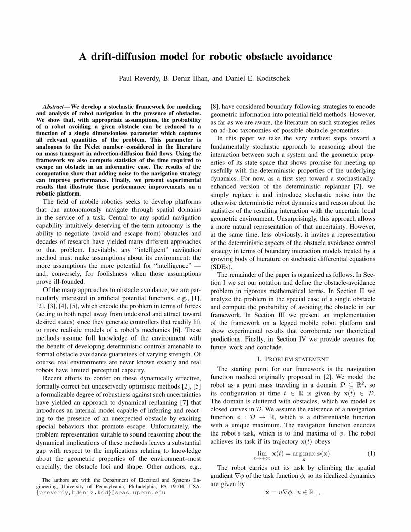
A drift-diffusion model for robotic obstacle avoidance

Paul Reverdy, B. Deniz Ilhan, and Daniel E. Koditschek

Abstract— We develop a stochastic framework for modelingand analysis of robot navigation in the presence of obstacles.We show that, with appropriate assumptions, the probabilityof a robot avoiding a given obstacle can be reduced to afunction of a single dimensionless parameter which capturesall relevant quantities of the problem. This parameter isanalogous to the Peclet number considered in the literatureon mass transport in advection-diffusion fluid flows. Using theframework we also compute statistics of the time required toescape an obstacle in an informative case. The results of thecomputation show that adding noise to the navigation strategycan improve performance. Finally, we present experimentalresults that illustrate these performance improvements on arobotic platform.

The field of mobile robotics seeks to develop platformsthat can autonomously navigate through spatial domainsin the service of a task. Central to any spatial navigationcapability intuitively deserving of the term autonomy is theability to negotiate (avoid and escape from) obstacles anddecades of research have yielded many different approachesto that problem. Inevitably, any “intelligent” navigationmethod must make assumptions about its environment: themore assumptions the more potential for “intelligence” —and, conversely, for foolishness when those assumptionsprove ill-founded.

Of the many approaches to obstacle avoidance, we are par-ticularly interested in artificial potential functions, e.g., [1],[2], [3], [4], [5], which encode the problem in terms of forces(acting to both repel away from undesired and attract towarddesired states) since they generate controllers that readily liftto more realistic models of a robot’s mechanics [6]. Thesemethods assume full knowledge of the environment withthe benefit of developing deterministic controls amenable toformal obstacle avoidance guarantees of varying strength. Ofcourse, real environments are never known exactly and realrobots have limited perceptual capacity.

Recent efforts to confer on these dynamically effective,formally correct but undeservedly optimistic methods [2], [5]a formalizable degree of robustness against such uncertaintieshave yielded an approach to dynamical replanning [7] thatintroduces an internal model capable of inferring and react-ing to the presence of an unexpected obstacle by excitingspecial behaviors that promote escape. Unfortunately, theproblem representation suitable to sound reasoning about thedynamical implications of these methods leaves a substantialgap with respect to the implications relating to knowledgeabout the geometric properties of the environment–mostcrucially, the obstacle loci and shape. Other authors, e.g.,

The authors are with the Department of Electrical and Systems En-gineering, University of Pennsylvania, Philadelphia, PA 19104, USA.{preverdy,bdeniz,kod}@seas.upenn.edu

[8], have considered boundary-following strategies to encodegeometric information into potential field methods. However,as far as we are aware, the literature on such strategies relieson ad-hoc taxonomies of possible obstacle geometries.

In this paper we take the very earliest steps toward afundamentally stochastic approach to reasoning about theinteraction between such a system and the geometric prop-erties of its state space that shows promise for meeting upusefully with the deterministic properties of the underlyingdynamics. For now, as a first step toward a stochastically-enhanced version of the deterministic replanner [7], wesimply replace it and introduce stochastic noise into theotherwise deterministic robot dynamics and reason about thestatistics of the resulting interaction with the uncertain localgeometric environment. Unsurprisingly, this approach allowsa more natural representation of that uncertainty. However,at the same time, less obviously, it invites a representationof the deterministic aspects of the obstacle avoidance controlstrategy in terms of boundary interaction models treated by agrowing body of literature on stochastic differential equations(SDEs).

The remainder of the paper is organized as follows. In Sec-tion I we set our notation and define the obstacle-avoidanceproblem in rigorous mathematical terms. In Section II weanalyze the problem in the special case of a single obstacleand compute the probability of avoiding the obstacle in ourframework. In Section III we present an implementationof the framework on a legged mobile robot platform andshow experimental results that corroborate our theoreticalpredictions. Finally, in Section IV we provide avenues forfuture work and conclude.

I. PROBLEM STATEMENT

The starting point for our framework is the navigationfunction method originally proposed in [2]. We model therobot as a point mass traveling in a domain D ⊆ R2, soits configuration at time t ∈ R is given by x(t) ∈ D.The domain is cluttered with obstacles, which we model asclosed curves in D. We assume the existence of a navigationfunction φ : D → R, which is a differentiable functionwith a unique maximum. The navigation function encodesthe robot’s task, which is to find maxima of φ. The robotachieves its task if its trajectory x(t) obeys

limt→+∞

x(t) = arg maxx

φ(x). (1)

The robot carries out its task by climbing the spatialgradient ∇φ of the task function φ, so its idealized dynamicsare given by

x = u∇φ, u ∈ R+,

where the quantity u controls the speed at which the robotclimbs the gradient. However, there are disturbances tothese idealized dynamics due to, e.g., issues measuring thegradient ∇φ, interactions with the environment, as wellas disturbances introduced as part of the control scheme.Denote the coordinates on D as (x, y) = x. We modelthe disturbance in each coordinate as a Wiener process ofstrength D(x) ∈ R+, and assume that the two processes areindependent. The process noise intensity is the sum of twoterms: D(x) = Da(x) + Dc(x), where Da(x) ∈ R+ is theambient noise due to the environment and Dc(x) ∈ R+ isthe control noise added added as part of the control strategy.

The noise-corrupted dynamics are described by the fol-lowing Ito stochastic differential equation (SDE)

dx =

[dxdy

]dt = u

[∂φ∂x∂φ∂y

]dt+D(x)

[dWt

dVt

], (2)

where D(x) is the strength of the disturbance at x ∈ D anddWt and dVt are independent Wiener increments. Dependen-cies in the disturbances can be modeled by making D(x)a positive-definite matrix-valued function of x. Standardreferences for the SDE methods used in this paper are thebooks [9] and [10].

Solving Equation (2) generates trajectories of a singleparticle. Solving the equation repeatedly from the sameinitial conditions generates different trajectories due to thestochastic nature of the dynamics. Alternatively, one canconsider the probability distribution p(x, t) of the state x(t)as a function of time t. The probability distribution is afunction that gives the probability of finding the robot ina set of states:

Pr [x(t) ∈ S] =

∫S

p(x, t)dx, (3)

where S ⊆ D is a subset of the state space.The time evolution of the distribution p induced by the

dynamics (2) is given by the following partial differentialequation:

∂p

∂t=

1

2∇ · (D(x)D(x)T∇p)− u∇φ · ∇p. (4)

Equation (4) is known as the Fokker-Planck equation [9],[10]. Equations of this form are studied in the literature onscalar transport phenomena under various names such as theadvection-diffusion equation and the drift-diffusion equation.

The following physical analogy is illustrative. Consider adrop of dye in a fluid flow. The function p(x, t) measuresthe concentration of dye at the spatial location x at time t.If the dye is initially concentrated at x0, the initial conditionfor the equation (4) is the Dirac delta function p(x, t0) =δ(x − x0). As time elapses, the dye moves with the fluid,which flows with local velocity ∇φ(x) and diffuses withcoefficient D(x). Transport due to the local velocity is calledadvection, or drift, while the spreading due to the D(x) termis called diffusion, and the two terms of the equation arereferred to accordingly.

The equations (2) and (4) define a stochastic dynamicalsystem where u is a control parameter. In future work, we

will leverage tools from the stochastic geometry literatureto derive ways to tune u such that the robot can navigatethrough a spatially-distributed obstacle field. A key next stepto developing this theory will be the extension of our modelto the case of multiple obstacles.

II. SINGLE OBSTACLE

In this section, we analyze the interaction of a particleobeying the stochastic dynamics (2) and a single obstacle,which we model as a closed curve in D. We develop a setof assumptions under which we can calculate the probabilityof escaping a single obstacle in closed form as a function ofa single dimensionless parameter.

A. Assumptions

We make the following assumptions to develop analyticaltools to study informative cases of the obstacle escapeproblem.

1) The coordinates are aligned with the local gradient∇φ,such that ∂φ/∂x = 1 is a constant and ∂φ/∂y = 0. Inother words, traveling in the +x direction is equivalentto climbing the (constant) local gradient.1

2) The diffusion tensor D(x) is diagonal and constant inx: D(x) = Diδij .

3) Diffusion only acts in the dimension orthogonal to thegradient, so D(x) has x component D1 = 0 and ycomponent D2 = D.

4) The particle interacts with obstacles through specularreflection: if, prior to the interaction it has momentump, after the interaction it will have momentum p′ =p− 2n(n · p), where n is the outward normal vectorto the surface of the obstacle at the point of contact.This is equivalent to assuming that the obstacles haveinfinite mass and that the particle-obstacle interactionis an elastic collision.

Specular reflection constitutes one of the two canonicaltypes of boundary conditions generally specified for stochas-tic differential equations (with absorption being the other[10]). More recent work, e.g., [11], [12], has consideredmore general boundary conditions that could model inelasticcollisions with a coefficient of restitution ε ∈ (0, 1). How-ever, the interpretation of these boundary conditions is morecomplicated and would require more detailed modeling of thephysical obstacle interaction. Therefore, in this preliminarystudy, we adopt the abstract reflecting boundary condition asthe most appropriate for developing analytical results withthe particle model considered here.

With these assumptions, the dynamics (2) reduce to

dx =

[xy

]dt =

[u0

]dt+

[0 00 D

] [dWt

dVt

]. (5)

The drift-diffusion equation (4) induced by (5) is

∂p

∂t=D2

2

∂2p

∂y2− u∂p

∂x. (6)

1This analytical simplification (guaranteed by the “flowbox” theorem ofdynamical systems to be possible in the neighborhood of any non-singularorbit) would not have any impact on the actual physical implementation.

We assume that the initial location of the particle is knownwith certainty to be x0 = (x0, y0) ∈ D, so the initialcondition for (6) is p(x, t = 0) = δ(x − x0). Finally, weassume that the speed u is constant.

In the absence of boundary conditions, the solution of (6)can be found in closed form, and is (cf. [9, (5.20)])

p(x, t) =1√

2πD2texp

(− (y − y0)2

2D2t

)δ(x− (x0 + ut)).

(7)The solution can be interpreted as follows. The particlemoves deterministically along the x coordinate with a con-stant velocity u and moves stochastically along the y coor-dinate according to a random walk. At time t, the particledistribution is Gaussian with center (x0+ut, y0) and standarddeviation D

√t.

For a given evolution time t the distribution has twocharacteristic lengths:

1) Advection length scale: ut2) Diffusion length scale: D

√t.

Their ratio, ut/D√t, is a form of the Peclet number [13],

which is a dimensionless quantity that measures the relativestrength of advection and diffusion. This ratio is a functionof evolution time t; if we specify an evolution time, weget a characteristic number that captures all the dimensionalvariables governing the dynamical behavior.

B. Probability of escaping a single obstacle

The dynamics (5) have a clear flow in the positive xdirection. We take advantage of this behavior to characterizeobstacles according to their geometry relative to the flow.Intuitively, the reflecting boundary condition specified inassumption 4) allows the particle to bounce off of obstaclesand in some cases escape an obstacle by moving aroundit. However, a particle will clearly not be able to escape allobstacles in this fashion. Consider, for example, the crescent-shaped obstacle shown in Figure 1-B. If the advection termdominates in the dynamics (5), then the particle will tend toget trapped by the obstacle.

The examples in Figure 1 illustrate that the important char-acteristic of an obstacle in this framework is the convexity ofits footprint with respect to the local advective flow. Looselyspeaking, an obstacle is convex with respect to the flow (5) ifthe obstacle appears convex to an observer looking at it fromthe upstream direction. An obstacle concave with respect tothe flow is defined analogously.

A B

r�

Fig. 1. Example obstacles placed in the flow described by the dynamics(5). Panel A: an obstacle that is convex with respect to the flow, and willnot trap a particle with D > 0. Panel B: An obstacle that is concave withrespect to the flow, and may trap a particle regardless of the value of D.

The definition of obstacle convexity can be made moreprecise in the following way. Define a section Σ transverseto the flow upstream of the obstacle. Consider the noise-free dynamics, i.e., (5) with D = 0. For each point x ∈ Σ,define g(x) as the time at which the solution to the noise-freedynamics with initial condition x first touches the obstacle.The convexity property of the obstacle can now be formallydefined as being inherited from that of the time-to-impactfunction, g.

If a particle following the dynamics (5) with D = 0evolves from an initial condition upstream of a concaveobstacle, it will eventually hit the obstacle and remain closeto the point of impact. Conversely, we define a particle tohave escaped an obstacle if its trajectory passes downstreamof the obstacle. On the basis of physical intuition andnumerical experiments, we argue that a particle following (5)with D > 0 will escape convex obstacles with probabilityone. This statement follows from the asymptotic behavior ofsolutions of (6), but that degree of formal development liesbeyond the scope of the present exploratory paper.

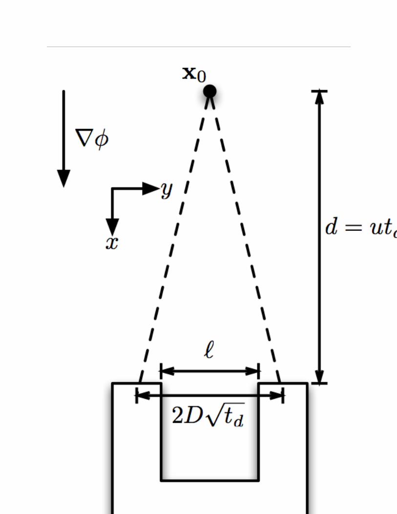
In contrast to convex obstacles, concave obstacles can trapparticles with positive probability. Therefore, we explore insomewhat greater detail the interplay between controlled driftand diffusion in the face of concavity. Figure 2 defines thequantities relevant to the interaction with a concave obstacle.The advection and diffusion length scales defined in theprevious section appear, as well as two geometric lengthscales: d is the distance between the initial position of theparticle and the front of the obstacle located downstream,and ` is the width of the concave section of the obstacle.Note that ` can be less than the width of the obstacle itself.For simplicity of exposition we assume that the obstacle hasa mirror symmetry over the y = y0 axis. The probability ofescape thus computed is a lower bound for the probabilityassociated with a non-symmetric obstacle with the samewidth `.

The geometric length scales allow us to compute theprobability that a particle obeying (5) will escape a givenconcave obstacle. We evolve the probability distribution (7)of the location of the particle until it reaches the front of theobstacle. This requires the particle to travel a distance d at aconstant speed u, which takes time td = d/u. This sets theevolution time for the advection and diffusion length scales.The particle’s location follows a Gaussian distribution withmean y0 and standard deviation σ = D

√td = D

√d/u.

The particle will move into the concave region of theobstacle and get trapped if it is at the edge of the concaveregion at time td, i.e., if its y coordinate is in the range(−`/2, `/2). Since the particle’s location is Gaussian dis-tributed, the probability that y is in this range, and thereforethat the particle will become trapped, can be calculated inclosed form. This yields π, the probability that the particlewill avoid the obstacle:

π = Pr [Avoid obstacle] = 2

(1− Φ

(Pe

2

)), (8)

where Pe =√

`2uD2d ≥ 0 is the Peclet number for the given

interaction and Φ : R→ [0, 1] is the cumulative distributionfunction for the standard normal (i.e., Gaussian) distribution.

x

y

`

r�

x0

d = utd

2Dp

td

Fig. 2. The geometry of interaction with a concave obstacle. There arethree characteristic lengths involved: d, D

√td, and `. The particle starts

at location x0, which is at a distance d from the obstacle, and travels ata constant speed u. This defines the time to interaction td through therelationship d = utd. At the interaction time, the effects of diffusion meanthe particle distribution has characteristic width D

√td. When the particle

interacts interacts with the obstacle, it will get trapped if its location fallsinside the concave footprint, which has width `.

Figure 3 compares the analytical avoidance probability (8)with the simulated avoidance probability computed from 100numerical simulations of the particle interaction depicted inFigure 2. The two avoidance probabilities match well upto moderate values of the diffusion coefficient D; for largevalues of D, there is more of a discrepancy, but this is likelydue to approximation effects in the simulation code.

C. Escape time

The primary objective in the single obstacle problem isescaping the obstacle, for which the probability of avoidance(8) gives a quantitative metric. Given that the particle escapesthe obstacle, a secondary objective is to do so quickly. Forthis objective a quantitative metric is time to escape, whichcan also be analyzed in our stochastic framework.

Consider again an obstacle interaction with geometry asin Figure 2. Define the random variable T as the first timeat which the particle passes beyond the face of the obstacle.

1 2 3 4 5 6 7 8 9 10

Diffusion coefficient, D

0.0

0.1

0.2

0.3

0.4

0.5

0.6

0.7

0.8

Pro

bab

ilit

y of

ob

stacl

e a

void

an

ce

Theoretical predictionNumerical simulation data

Fig. 3. Analytical vs. simulated obstacle avoidance probability for theconcave obstacle depicted in Figure 2. The theoretic analytical probabilityis given by (8), while the simulated probability (with approximate 95%confidence interval) is computed as the empirical avoidance probability from100 numerical simulations. The two quantities match well up to moderatevalues of the diffusion coefficient D.

That is,T = inf

τ≥0{x(τ) > 0},

where x(τ) is the x coordinate of the particle at time τ . Thequantity T is a random variable because of the stochasticnature of the dynamics. In general, T can have a complicateddistribution, which depends on the initial location of theparticle. Let T (x) represent the mean of T conditional onthe initial location being equal to x.

The function T (x) (and the higher-order moments ofT ) can be computed using a partial differential equationthat is closely related to the Fokker-Planck equation (4)[10, Section 6.6]. The partial differential equation can besolved analytically only in special cases, corresponding toobstacles with simple geometries. In more general cases,it can be solved numerically using finite element methods.An alternative method for finding the distribution of T isdirect simulation of individual trajectories. This method iscompletely general and can be thought of as a type of particlefilter method. In the following, we use direct simulation tostudy escape probability and escape time.

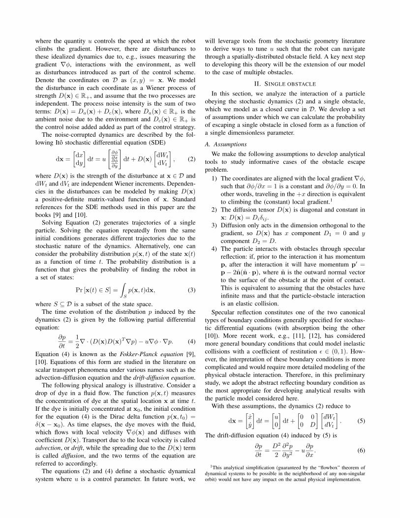
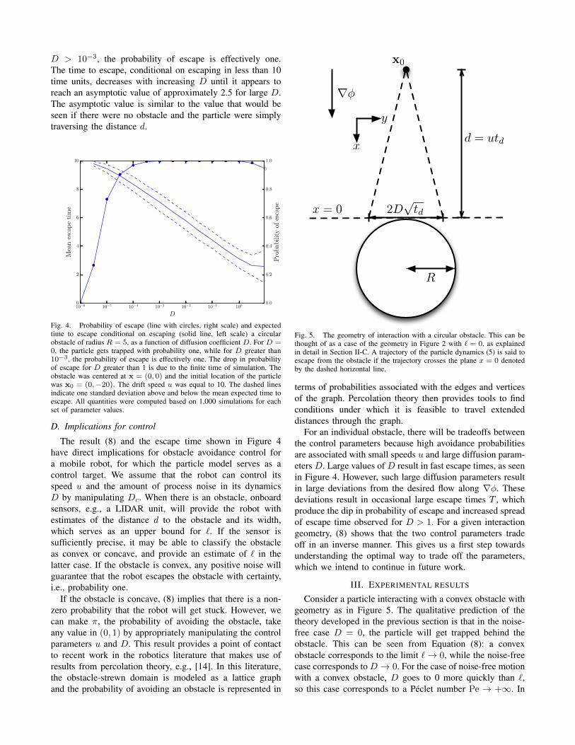
Figure 4 shows the probability of escape π and meanescape time T (x0) as a function of diffusion coefficientD for a particle obeying dynamics (5) interacting with acircular obstacle with the geometry depicted in Figure 5. Thisgeometry can be considered a special case of the geometrydepicted in Figure 2 with the length ` of the concave footprintbeing ` = 0. As argued above, the details of the obstaclegeometry outside the concave section of the footprint do notmatter so long as they are convex with respect to the driftflow ∇φ.

When D = 0, the particle hits the obstacle at the point(x, y) = (0, 0) and reflects directly along the direction inwhich it came, thereby getting trapped with probability one.For D > 0, the particle eventually escapes the obstacle,though the time to escape can be arbitrarily long. The figuredepicts probability of escape in less than 10 time units; for

D > 10−3, the probability of escape is effectively one.The time to escape, conditional on escaping in less than 10time units, decreases with increasing D until it appears toreach an asymptotic value of approximately 2.5 for large D.The asymptotic value is similar to the value that would beseen if there were no obstacle and the particle were simplytraversing the distance d.

10−6 10−5 10−4 10−3 10−2 10−1 100

D

0

2

4

6

8

10

Mea

nes

cap

eti

me

0.0

0.2

0.4

0.6

0.8

1.0

Pro

bab

ilit

yof

esca

pe

Fig. 4. Probability of escape (line with circles, right scale) and expectedtime to escape conditional on escaping (solid line, left scale) a circularobstacle of radius R = 5, as a function of diffusion coefficient D. For D =0, the particle gets trapped with probability one, while for D greater than10−3, the probability of escape is effectively one. The drop in probabilityof escape for D greater than 1 is due to the finite time of simulation. Theobstacle was centered at x = (0, 0) and the initial location of the particlewas x0 = (0,−20). The drift speed u was equal to 10. The dashed linesindicate one standard deviation above and below the mean expected time toescape. All quantities were computed based on 1,000 simulations for eachset of parameter values.

D. Implications for control

The result (8) and the escape time shown in Figure 4have direct implications for obstacle avoidance control fora mobile robot, for which the particle model serves as acontrol target. We assume that the robot can control itsspeed u and the amount of process noise in its dynamicsD by manipulating Dc. When there is an obstacle, onboardsensors, e.g., a LIDAR unit, will provide the robot withestimates of the distance d to the obstacle and its width,which serves as an upper bound for `. If the sensor issufficiently precise, it may be able to classify the obstacleas convex or concave, and provide an estimate of ` in thelatter case. If the obstacle is convex, any positive noise willguarantee that the robot escapes the obstacle with certainty,i.e., probability one.

If the obstacle is concave, (8) implies that there is a non-zero probability that the robot will get stuck. However, wecan make π, the probability of avoiding the obstacle, takeany value in (0, 1) by appropriately manipulating the controlparameters u and D. This result provides a point of contactto recent work in the robotics literature that makes use ofresults from percolation theory, e.g., [14]. In this literature,the obstacle-strewn domain is modeled as a lattice graphand the probability of avoiding an obstacle is represented in

r�

x

y

x = 0

x0

R

2Dp

td

d = utd

Fig. 5. The geometry of interaction with a circular obstacle. This can bethought of as a case of the geometry in Figure 2 with ` = 0, as explainedin detail in Section II-C. A trajectory of the particle dynamics (5) is said toescape from the obstacle if the trajectory crosses the plane x = 0 denotedby the dashed horizontal line.

terms of probabilities associated with the edges and verticesof the graph. Percolation theory then provides tools to findconditions under which it is feasible to travel extendeddistances through the graph.

For an individual obstacle, there will be tradeoffs betweenthe control parameters because high avoidance probabilitiesare associated with small speeds u and large diffusion param-eters D. Large values of D result in fast escape times, as seenin Figure 4. However, such large diffusion parameters resultin large deviations from the desired flow along ∇φ. Thesedeviations result in occasional large escape times T , whichproduce the dip in probability of escape and increased spreadof escape time observed for D > 1. For a given interactiongeometry, (8) shows that the two control parameters tradeoff in an inverse manner. This gives us a first step towardsunderstanding the optimal way to trade off the parameters,which we intend to continue in future work.

III. EXPERIMENTAL RESULTS

Consider a particle interacting with a convex obstacle withgeometry as in Figure 5. The qualitative prediction of thetheory developed in the previous section is that in the noise-free case D = 0, the particle will get trapped behind theobstacle. This can be seen from Equation (8): a convexobstacle corresponds to the limit `→ 0, while the noise-freecase corresponds to D → 0. For the case of noise-free motionwith a convex obstacle, D goes to 0 more quickly than `,so this case corresponds to a Peclet number Pe → +∞. In

contrast, in the case with noise D > 0, the Peclet numberobeys Pe → 0 and Equation (8) predicts that the particlewill eventually escape the obstacle. As shown in Figure 4, thetheory also predicts that in this case the mean time to escapedecreases sharply with increasing noise. In this section, wepresent results of robot experiments that corroborate thesequalitative predictions.

A. Implementation on RHex

To verify the qualitative predictions of the theory devel-oped above in the context of a physically interesting robot(rather than a more literal instantiation of the abstract pointparticle for which the theory and simulation are literallyapplicable), we implemented a version of the stochasticdynamics (5) on an X-RHex hexapedal robot [15]. The X-RHex robots have non-trivial dynamics [16] whose coarsehorizontal plane motion in slow gaits (e.g., up to two bodylengths per second) can be reasonably well approximated bya kinematic unicycle [17] and by a second order general-ization of such nonholonomically constrained models whenmoving at higher speeds [18]. For purposes of the presentexploratory paper, we used a gait slow enough to be usefullyabstracted by the kinematic unicycle, and applied a variantof the controller in [17] whose anchoring relation [19] tothe notional point-particle gradient dynamics posited in thispaper can be rigorously established [20].

However, because we are disinclined to allow our robotto actually collide and bounce off a physical obstacle, ourpoint particle gradient controller is rather more complicatedthan the simple constant-flow-with-elastic-collision modelunderlying the theoretical results presented above. Rather,we posit that the modified navigation function controller [7]implemented in these experiments introduces local determin-istic interactions with obstacles that would be better modeledby the case of a plastic collision — i.e., the case ε = 0in Section II-A, Assumption 4. Looking ahead to assessingthe efficacy of more sophisticated local replanners [7], weare pursuing the analysis of the more general “scattering”collision models discussed in that section. However, thesemore sophisticated analyses all lie beyond the scope of thepresent paper. In sum, the discrepancies between our actualrobot control strategy and the abstraction used to develop thetheory of Section II preclude any likelihood that quantitativepredictions from the stochastic theory could be directlycomparable to these experimental results. However, as wenow report, the qualitative predictions are encouraginglyreflected in these early empirical trials.

The implementation used for the robot experiments fol-lows an approach that was first introduced by Khatib [1]where the task to be executed is represented by an artificialpotential field composed of an attractive pole representing thegoal state and repelling regions representing the obstacles.An extension to this approach was developed by Borensteinand Koren [21] where the obstacles are represented bycertainty grids which enables a temporal filtering approachto obstacle detection. An alternative approach introducedby Borenstein and Koren [3] stems from some limitations

of the previous method and focuses on moving to emptyregions rather than being repelled by obstacle regions. Aprevious implementation on the RHex platform [22] utilizes asimilar approach. Our assumptions regarding obstacle shapeand distribution let us disregard the limitations described byBorenstein and Koren and implement a simple local repellingfield around obstacles where, with proper choice of controlparameters, any spurious fixed points introduced to the forcefield are guaranteed to be unstable [20].

B. Experimental setup

In our experiments we used a circular obstacle in thegeometry depicted in Figure 5. The effective radius of theobstacle was approximately R = 0.75 m, and the initiallocation of the center of the robot was at x0 = (−2.0, 0.0)m, which is equivalent to an initial distance d = 2.0 m. Thegradient field ∇φ was generated by placing a point attractorin the far distance directly in front of the robot’s initialposition, along with an immediate repeller located in theobstacle. The effective radius of the repeller was small, and isincluded in the effective radius of the obstacle. The resultinggradient field approximates the constant field assumed in thedynamics (5) to a degree of precision comparable to the otherexperimental uncertainties. Timing for runs was performedthrough manual control of logging software, which resultedin measurements of the time to escape that were accurate towithin 1 s.

As defined above, the process noise D was modeled as thesum of two terms: D = Da+Dc, where Da was the ambientnoise due to the environment and Dc was the control noiseadded as part of the control strategy. The ambient noise Da

is due to noise in the robot’s perceptual systems and variouscontrol loops. We manipulated the control noise Dc to havetwo values: either Dc = 0 or Dc =

√40 ≈ 6.3 m·s−1/2. We

did not directly measure nor manipulate the ambient noiseDa, but it can reasonably be assumed to have been smalland constant across the series of experiments. Importantly,the experimental results presented below imply that Da wasnon-zero.

C. Results

The experiments consist of a number of obstacle interac-tions for the two control noise cases: the noise-free caseDc = 0 and the noisy case Dc =

√40. For these first

efforts, we focused exclusively on the single circular convexobstacle, rather than a family of obstacles including bothconvex and concave examples; such a family will be thesubject of future work. Again, the noise values are notdirectly comparable to the diffusion coefficient D defined inSection II because of the details of the control strategy usedon the robot. The results presented in Table I show, however,that the experiments match the qualitative trend predicted inFigure 4: adding control noise results in a higher probabilityof escaping the obstacle and a shorter mean time to escapefor those runs that do escape.

In the noise-free case where Dc = 0, 50% of the runsresulted in the robot escaping the obstacle. In view of the

Noise-free, Dc = 0 Noisy, Dc > 0N = 8 runs N = 10 runs

Probability of escape 50% 100%Mean time to escape 45.08 s 8.860 sStandard deviation 13.94 s 0.5393 s

TABLE IEXPERIMENTAL RESULTS. THE NOISY CONTROL STRATEGY RESULTS IN

AVOIDING THE OBSTACLE MUCH MORE QUICKLY AND WITH

SIGNIFICANTLY HIGHER PROBABILITY.

results presented in Figure 4, this implies that the ambientnoise Da is small, resulting in an overall noise D = Da thatis comparable to the value of 10−5 that one can interpolatefrom Figure 4. Adding noise ensures that 100% of theempirical runs resulted in the robot escaping the obstacle.This corresponds to pushing the system into the regime onthe right hand side of Figure 4. The other benefit of thenoise can be seen in the mean time to escape: adding noiseresults in decreasing the mean time to escape by a factor ofapproximately five. This represents a substantial increase inobstacle avoidance performance.

Clearly the theory does not account for all of the empiricaltrends: for example, the empirical standard deviation oftime to escape decreases with increasing noise, while thesimulations based on the particle model presented in Figure4 show a standard deviation that is increasing with increasingnoise intensity. The intuition behind this trend is as follows.In the model, when a particle interacts with an obstacle,it can be reflected into the direction opposite the desireddirection of motion. When this occurs, the particle takeslonger to escape the obstacle. The control noise injectsmomentum into the particle, so larger noise intensities resultin more energetic reflecting interactions with the obstacle andlarger standard deviations of the escape time. This energeticreflecting behavior does not occur in the physical experiment,showing a limitation of the reflecting boundary conditionmodel. More detailed modeling of the robot-obstacle inter-action is required to better match theory and experiment.This modeling will be the subject of future work.

IV. CONCLUSIONS

In this paper, we have presented a simple stochastic modelfor analyzing robot navigation in the presence of isolatedobstacles. Pairing a very simple geometric model with thesimple stochastic differential equation affords a characteriza-tion of the types of obstacles likely to trap a robot in terms oftheir convexity along with a closed form expression for theprobability of escape from them. Simulation of this modelyields numerical estimates of the expected time to escape(conditioned on escape) from the obstacle. Our simulationstudy suggests that adding noise to a simple navigationfunction-based obstacle avoidance approach can significantlydecrease the time to escape, thereby substantially improvingperformance. Finally, a physical implementation on a mobilerobotic platform yields empirical results whose trends matchtheoretical predictions.

Our stochastic approach also allows us to connect to recentwork in robotics utilizing results from stochastic geometry.Notably, we aim to leverage the work of Karaman and

Frazzoli [14], who studied the motion planning problem fora vehicle obeying simple first-order integrator dynamics ina Poisson forest, i.e., an environment in which obstaclesoccur according to a spatial Poisson process. They provedthat there is a phase change in the qualitative nature of themotion planning problem as a function of the vehicle’s speed.Below a critical value of the speed, there exist planners thatcan navigate arbitrarily far through the forest. Above thecritical value, no motion planner can avoid collisions: for anyplanner, a collision with an obstacle will inevitably happenin finite time. We hope to develop similar results for vehiclesusing navigation functions.

The work presented in this paper represents a first steptowards a more general theory of navigation functions foruncertain environments. As mentioned previously, a key nextstep to developing this theory will be the extension of ourmodel to the case of multiple obstacles. For this case wewill rely on several tools from statistics, specifically the fieldof stochastic geometry. Hard-core point processes [23], [24]will provide the tools to model fields of obstacles, whilepercolation theory results, e.g., [14], [25] will provide thetools to develop control schemes to navigate through theseobstacle fields.

As was shown by the comparison between our theoreticalpredictions and empirical data, further modeling needs to bedone to understand how our simple model works when it isimplemented in a physical robot. The methods of stochasticLyapunov functions [26] are likely to be important toolsfor this work. The resulting theory of navigation functionsfor uncertain environments will provide tools to developpractical controllers for mobile robots that have provablenavigation performance guarantees.

ACKNOWLEDGEMENT

This work was funded in part by the Air Force Office ofScientific Research under the MURI FA9550-10-1-0567. Theauthors thank D. Guralnik for discussions on the generalizeddefinition of obstacle convexity developed in Section II-B, and the various reviewers for their comments, whichstrengthened the paper.

REFERENCES

[1] O. Khatib. Real-time obstacle avoidance for manipulators and mobilerobots. The International Journal of Robotics Research, 5(1):90–98,1986.

[2] D. E. Koditschek. Exact robot navigation by means of potentialfunctions: Some topological considerations. In Proceedings of theIEEE International Conference on Robotics and Automation, 1987.

[3] J. Borenstein and Y. Koren. The vector field histogram-fast obstacleavoidance for mobile robots. IEEE Transactions on Robotics andAutomation, 7(3):278–288, 1991.

[4] J.-O. Kim and P. K. Khosla. Real-time obstacle avoidance usingharmonic potential functions. IEEE Transactions on Robotics andAutomation, 8(3):338–349, 1992.

[5] E. Rimon and D. E. Koditschek. Exact robot navigation using artificialpotential fields. IEEE Transactions on Robotics and Automation,8(5):501–518, 1992.

[6] D. E. Koditschek. The control of natural motion in mechanicalsystems. Journal of Dynamic Systems, Measurement, and Control,113:547–551, 1991.

[7] S. Revzen, B. D. Ilhan, and D. E. Koditschek. Dynamical trajectoryreplanning for uncertain environments. In Proceedings of the 51stIEEE Annual Conference on Decision and Control, pages 3476–3483,2012.

[8] M. Trevisan, M. A. P. Idiart, E. Prestes, and P. M. Engel. Exploratorynavigation based on dynamical boundary value problems. Journal ofIntelligent and Robotic Systems, 45(2):101–114, 2006.

[9] H. Risken. The Fokker-Planck Equation. Springer, 1984.[10] C. Gardiner. Stochastic Methods: A Handbook for the Natural and

Social Sciences, volume 13 of Springer Series in Synergetics. Springer,4th edition, 2009.

[11] P. Szymczak and A. J. C. Ladd. Boundary conditions for stochastic so-lutions of the convection-diffusion equation. Phys. Rev. E, 68:036704,2003.

[12] A Singer, Z. Schuss, A. Osipov, and D. Holcman. Partially reflecteddiffusion. SIAM Journal on Applied Mathematics, 68(3):844–868,2008.

[13] M. Huysmans and A. Dassargues. Review of the use of Peclet numbersto determine the relative importance of advection and diffusion in lowpermeability environments. Hydrogeology Journal, 13(5-6):895–904,2005.

[14] S. Karaman and E. Frazzoli. High-speed flight in an ergodic forest.In IEEE International Conference on Robotics and Automation, pages2899–2906. IEEE, 2012.

[15] K. C. Galloway, G. C. Haynes, B. D. Ilhan, A. M. Johnson, R. Knopf,G. Lynch, P. Plotnich, M. White, and D. E. Koditschek. X-RHex:A highly mobile hexapedal robot for sensorimotor tasks. Technicalreport, University of Pennsylvania, 2010.

[16] J. D. Weingarten, R. E. Groff, and D. E. Koditschek. A frameworkfor the coordination of legged robot gaits. In Robotics, Automationand Mechatronics, 2004 IEEE Conference on, volume 2, 2004.

[17] G. A. D. Lopes and D. E. Koditschek. Visual servoing for nonholo-nomically constrained three degree of freedom kinematic systems. TheInternational Journal of Robotics Research, 26(7):715–736, 2007.

[18] A. De, K.S. Bayer, and D.E. Koditschek. Active sensing for dynamic,non-holonomic, robust visual servoing. In 2014 IEEE InternationalConference on Robotics and Automation (ICRA), pages 6192–6198,May 2014.

[19] R. Full and D. Koditschek. Templates and anchors: Neuromechanicalhypotheses of legged locomotion on land. J. of Experimental Biology,202(23):3325–3332, 1999.

[20] B. D. Ilhan, A. M. Johnson, and D. E. Koditschek. Autonomous leggedhill ascent. (in preparation).

[21] J. Borenstein and Y. Koren. Real-time obstacle avoidance for fastmobile robots. Systems, Man and Cybernetics, IEEE Transactions on,19(5):1179–1187, 1989.

[22] A. M. Johnson, M. T. Hale, G. C. Haynes, and D. E. Koditschek.Autonomous legged hill and stairwell ascent. In Safety, Security,and Rescue Robotics (SSRR), 2011 IEEE International Symposiumon, 2011.

[23] D. Stoyan and H. Stoyan. On one of Matern’s hard-core point processmodels. Mathematische Nachrichten, 122(1):205–214, 1985.

[24] J. Teichmann, F. Ballani, and K.G. van den Boogaart. Generalizationsof Matern’s hard-core point processes. Spatial Statistics, 3(0):33–53,2013.

[25] S. N. Chiu, D. Stoyan, W. S. Kendall, and J. Mecke. Stochasticgeometry and its applications. John Wiley & Sons, 2013.

[26] H. J. Kushner. Stochastic stability. In Lecture Notes in Mathematics294. Springer-Verlag, New York, 1972.