a dual method of empirically evaluating dynamic

A Dual Method of Empirically EvaluatingDynamic Competitive Equilibrium Models with Distortionary Taxes,including Applications to the Great Depression and World War II*

by Casey B. Mulligan

University of Chicago and NBER

October 2000

Abstract

I prove some theorems for competitive equilibria in the presence of distortionary taxes andother restraints of trade, and use those theorems to motivate an algorithm for (exactly) computingand empirically evaluating competitive equilibria in dynamic economies. Although its economicsis relatively sophisticated, the algorithm is so computationally economical that it can beimplemented with a few lines in a spreadsheet. Although a competitive equilibrium modelsinteractions between all sectors, all consumer types, and all time periods, I show how my algorithmpermits separate empirical evaluation of these pieces of the model and hence is practical even whenvery little data is available. For similar reasons, these evaluations are not particularly sensitive tohow data is partitioned into "trends" and "cycles."

I then compute a real business cycle model with distortionary taxes that fits aggregate U.S.time series for the period 1929-50 and conclude that, if it is to explain aggregate behavior during theperiod, government policy must have heavily taxed labor income during the Great Depression andlightly taxed it during the war. In other words, the challenge for the competitive equilibriumapproach is not so much why output might change over time, but why the marginal product of laborand the marginal value of leisure diverged so much and why that wedge persisted so long. In thissense, explaining aggregate behavior during the period has been reduced to a public financequestion – were actual government policies distorting behavior in the same direction and magnitudeas government policies in the model?

* I appreciate the comments of Jess Gaspar, Bob Lucas, Jeff Russell, GSB macro luncheaters, and Economics 332 students, and the research assistance of Fabian Lange.

Table of Contents

I. Introduction 1

II. Competitive Equilibria with Distortionary Taxes 6Setup of the Model 6

Consumers 6Firms and Distortionary Taxes 7The Government 8Resource Balance Constraints 9Definition of a Competitive Equilibrium 9

Problems with the Primal Approach 10

III. The Dual Procedure for Computing and Evaluating the Model 12"Demand" and "Supply" Prices 13

Consumer Problem 13Firms 13

"Tax Wedges" 14

IV. Application to the Great Depression and WWII 16A Real Business Cycle Model with Labor and Capital Income Taxes as a Special Case 16

Simulated Policies 19Understanding the Great Depression 23

Productivity Shocks Cannot Explain 1929-33, or 1933-39 24Personal Income Taxes are not an Important Part of the Labor-Leisure Distortion 24

How Much Can International Trade Explain? 25Labor Market Regulations 27Can Monopoly Unions be Part of the Story? 28What about Monetary Shocks? 32

Intertemporal Distortions During the Period 33

V. Conclusions 34Understanding the American Economy 1929-50 35Lessons for Other Applications 36Forecasting vs. Empirical Evaluation 37

VI. Appendix: Data and Calculations for the period 1929-50 37

VII. References 38

I. Introduction

Explaining aggregate measures of behavior, such as employment, output, consumption, and

investment, has for decades been one of the prime interests of macroeconomists, and others.

Almost as old is the question of how much aggregate behavior might be explained by private sector

impulses (in modem parlance: tastes, technology, market structure, and demographic shocks) rather

than public sector impulses such as government regulations, taxes, and subsidies. Somewhat more

recent are attempts to model private sector behavior as a dynamic competitive equilibrium, and

Kydland and Prescott (1982) is one rather successful one.

This paper is about the interaction between the time series data, construction of competitive

models of private behavior, and construction of models of government policy. I suggest that the

form of this interaction found in the literature is not computationally economical, requires a lot of

accurate data, and obscures the public finance dimension of the problem. I suggest another

procedure that improves in these dimensions and, assuming both procedures were carefully

executed and economically comparable, both arrive at the same conclusions.

One common, and understandable, procedure for constructing competitive equilibrium

explanations of aggregate behavior proceeds as follows:

(i) write down a model for government policy (eg., a set of taxes, transfers, and

regulations)

(ii) write down a model for private sector behavior, including responses to the modeled

government policies

(iii) choose functional forms and numerical parameters for the model of the private

sector (eg., rate of time preference, elasticities of substitution in preferences,

elasticities of substitution in production)

(iv) choose numerical values for the government policy parameters (a) based on some

observations of government policy and (b) so that the model government budget

constraint balances in step (v)

Equilibria with Distortions - 2

(v) compute a competitive equilibrium (eg., time series for employment, consumption,

interest rates, etc.)

(vi) compare the equilibrium quantities (and perhaps prices) to observed quantities (and

perhaps prices)

Steps (i) - (vi) might be done once, in which case the procedure is called "simulation," and the

success of the model might be judged on step (vi)'s metric of the proximity of simulated and

observed quantities. This is the approach, for example, of Burnside et al (2000) and, essentially,

Mulligan (1998), who conclude that a neoclassical model cannot explain some time series

comovements of employment and government expenditure, and Cole and Ohanian (1999) who

suggest that fiscal policy cannot explain the Great Depression. Steps (iii) - (vi) might be done

many times, perhaps with the objective of choosing numerical values for the private sector

parameters in order to maximize step (vi) 's metric of the proximity of simulated and observed

quantities, in which case the procedure is called "estimation." This is the approach, for example,

of Hansen and Sargent's (1991, Chapter 7) study of recursive linear competitive equilibrium models.

In either procedure, step (v) - computing quantities and prices that maximize utility, maximize

profits, and balance the government budget given numerical values for government policy - is not

an easy one, especially when government policy is distortionary. Indeed, this step can be so

difficult that many taking the competitive equilibrium approach (eg., Braun and McGratten 1993,

Ohanian 1993) are tempted to ignore the distortionary effects of taxes, and nearly all ignore the

distortionary effects of business, labor and product regulations. Even when distortionary taxes are

included in the model, it is difficult to understand F - namely how changes in private sector

parameters or government policies affect equilibrium quantities and prices.

My approach is not to advocate "simulation" versus "estimation," but rather to change steps

(iv)-(vi) in order to simplify computation and data requirements by orders of magnitude, and to

highlight the public finance of the problem. Here are my proposed steps:

write down a model for government policy (eg., a set of taxes, transfers, and

regulations)

(ii) write down a model for private sector behavior, including responses to the modeled

government policies

(iii) choose functional forms and numerical parameters for the model of the private


sector (eg., rate of time preference, elasticities of substitution in preferences,

elasticities of substitution in production)

(iv)' use observed quantities to compute marginal rates of substitution and

transformation

(v) ' use the competitive equilibrium conditions, and the results from (iv) ' , to compute

numerical values for the government policy parameters, and perhaps prices

(vi)' compare the equilibrium policies (and perhaps prices) to observed policies (and

perhaps prices)

Notice how I have left (i)- (iii) intact, changing only (iv)-(vi). In particular, I propose to feed

observed quantities into the model to infer policies, rather than feeding policies into the model to

infer quantities. For this reason, I refer to (i)- (vi) as the "primal" or "policy-quantity" approach

and my approach (i)- (vi) ' as the "dual" or "quantity-policy" approach, and highlight their

differences in Figure 1.

=numericalmodel ofprivate

Kbehavior/

PRAY NA.equilibrium

exists

HOPEcomputer

program writtencorrectly

(PC p*) =FCC), F) =simulatedprices &quantities

Primal

Kr observedgovernment

policies


Duale =

numericalmodel ofprivate

Kb ehavioy

\4t

X =observed.cluantitiesy

tcr* *) =

G(j8, pX) =

policies &prices

consistentwith equil.

WRY tounderstand F cf(IX*, X, Li*, =

simulatedprices &quantities

compared withobservation

Dr) ry P*, =simulatedpolicies &

pricescompared with

observationFigure 1 Overview of the Primal and Dual Approaches

We see in the Figure's left panel that the primal approach uses a numerical model of private

behavior and observed policies to simulate quantities and prices, and the red ovals emphasize some

of the practical difficulties with the approach. As shown in the right panel, the dual approach uses

a numerical model of private behavior and observed quantities to simulate policies and prices.

As in the primal approach, the dual approach has both simulation and estimation versions.

Steps (i)- (vi) ' could be done once (aka, "simulation") or steps (iii) - (vi) ' might be done many

times, perhaps with the objective of choosing numerical values for the private sector parameters


in order to maximize step (vi) "s metric of the proximity of simulated and observed policies (aka,

"estimation"). In either procedure, step (v)' – computing policies that satisfy equilibrium

conditions given observed quantities – is a trivial one. Indeed, estimation is much more economical

with my dual approach than with the primal approach because performing step (v) ' many times is

much easier than performing step (v) many times.

I expose the computational simplicity of the dual approach by proving three propositions.

The first shows that, given a model of private sector behavior and observed quantities, a policy

consistent with competitive equilibrium can be computed two first order conditions at a time, and

in any order. The second proposition shows that there is one and only one set of government

policies that is consistent with a competitive equilibrium. It is well known that analogous results

cannot be proven for the primal approach because there can be zero, or multiple, equilibrium

responses to a given policy (the "Laffer curve" characterizes some of the well known examples of

nonunique or nonexistent competitive equilibria), and the equilibrium quantity in any one sector

at any one date depends on policies and technologies in all sectors at all dates. Hence, the dual

approach does not present "equilibrium choice" or nonexistence problems, and does not require

much accurate data.

The paper then uses my procedure to "explain" the period 1929-50 with a real business cycle

model. The calculations are so simple that they are reported in a self-contained appendix for easy

verification by the interested reader. I show that, in order for the real business cycle model to

explain aggregate behavior during the period, marginal labor income tax rates must have been quite

high during the depression and quite low during the war. Since it appears that marginal labor

income tax rates had a different history, I conclude that the real business cycle model cannot

explain why there was so little employment during the Depression and so much during the War.

Perhaps another defensible conclusion is that marginal labor income tax rates did have a history

like that generated by the model, and that the usual measures of marginal tax rates are not

capturing all of the distortions introduced by government regulations, taxes, and subsidies during

the period. Under this interpretation of my results, explaining the period 1929-50 is reduced to the

public finance problem of identifying and quantifying the various government policies driving a

wedge between labor supply and labor demand, and showing how actual marginal tax rates had a

history like that generated by the model.


II. Competitive Equilibria with Distortionary Taxes

HA. Setup of the Model

There are a continuum of infinitely lived consumers and firms, each taking prices and policy

parameters as given. Consumers are partitioned into h=1,...,H (equally populated) types according

to the productivity of their labor, their preferences and their treatment by the government. There

are M capital goods, which are used together with labor to produce more capital goods or to

produce the N consumption goods. Any firm produces only one of these M-FN goods; firms are

indexed by their sectorF-1,...(M+N) with the first Nsectors producing consumption goods, and the

rest producing capital goods. Since the economy is assumed to be competitive the ownership of

capital does not affect the allocation in the economy. For convenience I assume that all capital is

owned by the firm producing it and rented out to the other firms for production purposes.

Vectors are denoted by underlined letter: x, and are column vectors. Matrices are denoted

by capped letters: x . I use ;i= to denote multiplication element-by-element and ® for Kronecker

products. Let X I stand for the vector of reciprocals of x.

Time is discrete and indexed by t = 0, ... . Consumption good prices, gross of taxes, are

given by: p(t) = [p1 (t), p2 (t),... px (t)I'

II.A.1 Consumers

The consumption of the N consumption goods by individual h is given by the vector

C h (t) = (0,4 (t),...chh, (Of .

Aggregate consumption of the economy is given by c(t) h ch (t) . Total labor supplied

by the household is e (0= M+N

/=I

L"(

t) and C (t) denotes the labor by h to sector i. The vector of

ownership shares by h of the N+M firms is given by ah [alh ,a2h ,..., a + . The interest rate

is given by q(t)

Preferences are governed by:


rt_o f1 ,tt h (c h (t), Lh (t), t)

The budget constraint is given by:

I:o ff'„, (1+ q(s)) -1 [Wh (t)Lh(t)- p(01 c h (t)+ V h (01+ Ge l = 0 (2)

where z is the value at date zero of the firms and V h (t) denotes the lump sum transfers at date

t.

The resource constraint of the individual can also be expressed using a series of constraints

as follows:

(i)e (i) Vh (t)+ a h (t) = p(t)' ch (t) + 1+ q(t + 1)] -1 a h (t + 1) t 0,...,00 (3)

a h (0) = alnz

where WI (t) and ah (t) are scalars denoting household h's date t wage rate and asset holdings.

II.A.2 Firms and Distortionary Taxes

The production functions are given by f, (K, (t), L, (t), t) where

K ,(t) [K,N+ ' (t) KN+2 (t),. , Ke itl+N (01 and L i ( )= , (01 arethevectors

of capital and labor inputs used by firm i at date t. (t) will denote the date t aggregate amount

of type i capital.

The rental rate vectors of inputs at date t are given by

r(t) = [r N+1 (0,7, 7%7+2 (t),...r M+N and w(t) = [w1 (t), w2 (t), . w" (t)]'

In sector i taxes are levied on labor at the rates ,(t) = [r (t), 22 (t),...,r (t)I , and

on capital inputs at rates y(t) = [y N (0 ,y N+4 (t) 7N+ M t)i The input prices faced by


firms are then

i . (0= r(t)*[I + y(t)] and 1113i (t) w(t)* i(t)]

The objective in the consumption good sector is:

zi (t)= max[ p; (t)f,(K1(t),L1(t),t)— 7(0' K1 0)— w i (0' L1 (t)] (4)

i = 1, , N and t 0, ... ,00

The problem in the production goods sector can be expressed recursively as

r` (OK' (0- it OF KE W - w,(0' L,(t)V (K` (t)) -= max

{ 1C(0,1,( 01 + q(0) -1 V (K` (t+ 1))

s.t. + 1) = f (Ki(0,4(t),t) + (1- 4)K' (t) (6)

K` (0) = 1(;) = N + 1, N + M

The value of the firms at date t is given by z(t) [z1 (t),Z2 (0, ..., ZA,± (0}

In this set up the investment by firms is reversible. The production of capital and

consumption goods however is restricted to be non-negative, i.e. f (K1 (t), Li (t),t) 0 V t, i .

An interior solution is assumed to hold, although see Houthakker (1995) , Mulligan (1999) , or

Mulligan (2000) for some discrete-choice interpretations of the "interior" conditions.

II.A.3. The Government

The government budget constraint is given by:

g(t)' p(t) = [y W I K (01 r(t)+Liv:i m - L, (t)fw(t) — V h MI (7)

where go)_ N(01 is the vector of government consumption. This constraint

simply says that government spending (consumption and net transfers) equals the sum of labor and

capital income taxes.

(5)


II.A.4 Resource Balance Constraints

Markets for consumer goods, capital goods, labor, and assets "clear" at each date. In other

words, government and private purchases equal output in each of the N consumption good sectors,

capital demanded by firms equal supply (capital type-by-type), labor demanded by firms equal

supply (labor type-by-type), and net household asset holdings equal the value of the firm sector.

Algebraically, market clearing implies (8)- (11).

g(t ) + c(t) . y N ( t ) = y N (t)T with y, (t) = f (K, (t ), L; (t), t) V t (8)

K` (t) = E Ki (t) , i = N + 1, N+ M, V t (9)

[LI (t), L2 (0, ... LH (t)T = N^ML,(t), V t (10)

E:v.=t iwz, (t) E h a h (t), Vt (11)

II.A.4 Definition of a Competitive Equilibrium

Given a policy sequence {g(t ), 7 (t), { h (t)} Hh_1 , fr i (t)I NIt hl r_o , initial capital stocks K0 and

initial ownership shares {a il hll_. 1 , a competitive equilibrium is given by quantity

sequences { { Lh (t),a h (t), c h (01,,HH ,{K'(0}7INA4+; {K,(t), L, (0} }°,1 0 , price sequences

{p(t),w(t),t- (t),q(0) and a sequence of firm values {z(t)} 7,0 such that:

(iv) { {Lh (t),a b (t), ch (t)},t )°,10 max mize (1) subject to (2) (or (3)) for all h

(v) {K,(t),1,1(t)}7=11 7, 0 maximize (4) for 1=1,...,Nand all t

{{K,(0, L, j /to maximize (5) for i=N+1,...,N+M


(vi) z,(t) 0

z,(t) =

for all i=1,„„N and all t

q(s)}-I (1– (5)s ti;(t)K' (t) for i=N+1,...,N+M and for all t

(vii) (7) - 01) hold at all t

(i) requires that households willingly consume the equilibrium consumption bundle, willingly hold

equilibrium assets, and willingly supply equilibrium labor. (ii) requires each type of firm to

willingly demand the equilibrium inputs. (iii) is a free-entry condition, and requires that firms are

only valued at the value of their assets. (iv) says the government budget constraint must hold and

all markets clear.

ILK Problems with the Primal Approach

Proposition la Given a policy sequence {g(t),{v h } hll_1 , {y (t), 1 (01 N:1 1" rt=o , initial

in IIcapital stocks Ko and intial ownership shares la } h,i , a competitive equilibrium may not exist.

Proof (by example) Consider a 1 household, 1 good economy without capital and with a policy

having no government consumption, no capital taxes:

g(t) = y(t) = 0 and v(t) = v * , as well as, r(t) r * This implies from the gov't BC that:

V * rL(t) - w(t) . (12)

Taking v* and t * as given the household problem yields a labor supply function:

L(t)= L(w(t); 2* ,v*) 03)

Unless the relation (12) and (13) intersect in the positive quadrant this economy does not admit an

equilibrium.


The existence problem is more severe than suggested by proposition la: even if part of the

policy sequence is treated as a free parameter, there are situations where no competitive

equilibrium exists. This is outlined in proposition lb:

Proposition lb Given a policy sequence Ig(t), O h (01 1;1, , {y (0} 1, 1/4t; "I; 0 , initial capital stocks

1-1K0 and intial ownership shares {a there might not exist a sequence fr ,( )Eviiiirro thatir=1

admits a competitive equilibrium.

Proof (by example) Consider a 1 household, 1 good economy without capital with the policy g(t)

= y (t) = 0 and v(t) . Also consider preferences that admit a (monotone, continuous) inverse

labor supply function s.t. (L=0 ,t) =0 and a production function s.t. the inverse (monotone,

continuous) labor demand function has w° (L=0 ,t) a.. Then in equilibrium the tax revenue is given

by the area T (t)w* (t) * L* (t). Continuity implies that this area is bounded by the area A between

the inverse supply and demand function and is thus finite. Thus for any v* > A , there are no tax

rates compatible with a competitive equilibrium.

Here the labor tax rate is taken as a free parameter, and only government spending,

transfers and capital taxes are taken as given. Still it is easy to construct an example in which for

the given policy sequences there does not exist a equilibrium-compatible labor tax rate. Similar

examples can be constructed for cases in which other subsets of the policy sequence are labeled

'free parameters' and givens. Note the proof given for proposition lb is a simple case of an economy

with a continuous, bounded Laffer curve. Any policy allocation requiring revenues greater than the

bound on the Laffer curve can not possibly be supported.

A similar idea can be used to prove an analogous idea for the multiple equilibrium case, as

in Proposition 2.

Proposition 2 @ forthcoming @


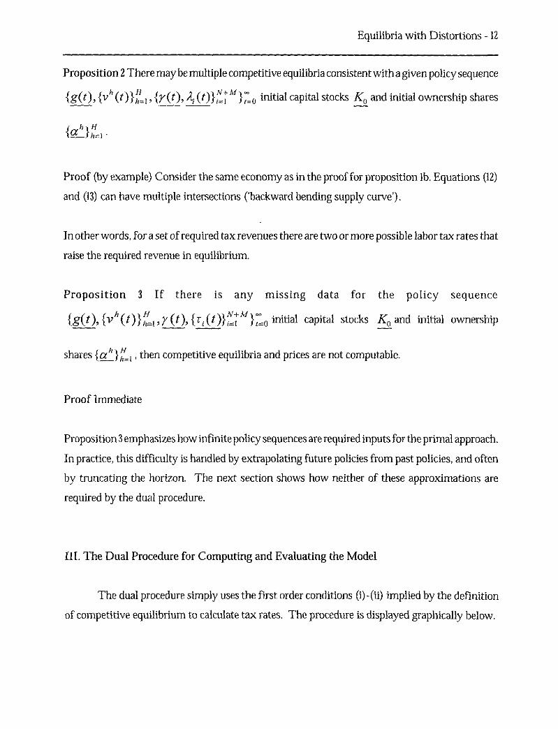
Proposition 2 There maybe multiple competitive equilibria consistent with a given policy sequence

{g(t), {vh (t)} 1,H_ I , {y (t), A7 ,A1_+:1 _ o initial capital stocks K0 and initial ownership shares

a hr„).hr

Proof (by example) Consider the same economy as in the proof for proposition lb. Equations (12)

and (13) can have multiple intersections (backward bending supply curve') .

In other words, for a set of required tax revenues there are two or more possible labor tax rates that

raise the required revenue in equilibrium.

Proposition 3 If there is any missing data for the policy sequence

{g(t), {1, 11 (0} iHri ,r (t), {Z" 1 (0} ,N_I A 17_0 initial capital stocks K0 and initial ownership

shares {a il { hi/ , then competitive equilibria and prices are not computable.

Proof Immediate

Proposition 3 emphasizes how infinite policy sequences are required inputs for the primal approach.

In practice, this difficulty is handled by extrapolating future policies from past policies, and often

by truncating the horizon. The next section shows how neither of these approximations are

required by the dual procedure.

III. The Dual Procedure for Computing and Evaluating the Model

The dual procedure simply uses the first order conditions (i)-(ii) implied by the definition

of competitive equilibrium to calculate tax rates. The procedure is displayed graphically below.


III.A."Demand" and "Supply" Prices

III.A.1 Consumer Problem

Let mrs(cjh (t), Lh (s)) = log(VW (0, 11, (0,t) cycijoau' (ch (s), e(s), ․)1 &e (s) , With a known utility

function, and known date t quantities, mrs can readily be calculated. Item (i) of the definition of

competitive equilibrium requires that consumers willingly demand the equilibrium quantities. If

these quantities are positive, then (i) implies the first order condition equating marginal rates of

substitution to the relative after-tax price of goods (note normalization of

pi (t)=1Vt= ):

mrs(c,(t), e (t)) = log(p, (t))- log(w h (t)) N [C.1]

mrs(c,(0,c i (s)) kt log(1+ q(k))– E sk _ o log(1+ q(k)) [C.2]

Equations [C.11 are the within-period first order conditions and [CA the between-period

conditions. These conditions are related to the within- and between- period conditions for firms,

as shown below.

III.A.2 Firms

Item (ii) of the definition of competitive equilibrium requires that firms willingly demand

the equilibrium quantities. If these quantities are positive, then (ii) implies the first order condition

equating marginal products to the net-of-tax input rental rates:

c5f,(K,(t), ,(t), t)\

81,t (t) )log - log(wh+ log(1 + r (0)- log(p,( )) [F1]

=1, h = 1, ...,H


6f,(1C 1 (t), L,(1),t)log - log(w h (t))+ loge + r (t))- log(2, (t)) [F.2]

OL, (t)

i

i g(KI (t), Li e), 0\

N+1,...,N+M,h= 1, ...,H

log - log(r, (t))+ loge + y (t))- log(p,(0) [F.3]81C; (t)

1-- 1, j = N+1, ...,N+M

logSl(K1 (t), Li(t),

- log(r, ( ))+ loge + (t)) - log(,, (t)) [F.4](t)

= ...,N+M, j = N+1,

where 2, (t) = IT II ss=1 mr0 (1 +q(t + m)) -1 r, (t + s)(1 — 5 ,)s represent the PDV of a unit

of capital of type 1.

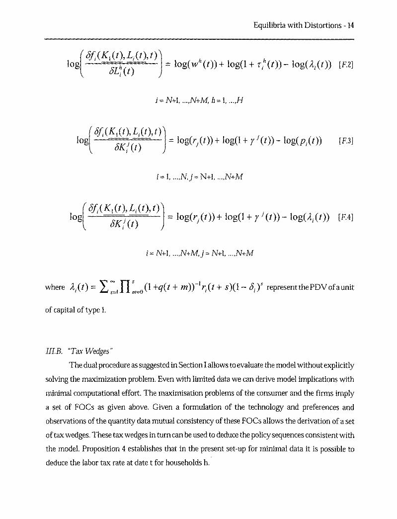
III.B. "Tax Wedges"

The dual procedure as suggested in Section I allows to evaluate the model without explicitly

solving the maximization problem. Even with limited data we can derive model implications with

minimal computational effort. The maximisation problems of the consumer and the firms imply

a set of FOCs as given above. Given a formulation of the technology and preferences and

observations of the quantity data mutual consistency of these FOCs allows the derivation of a set

of tax wedges. These tax wedges in turn can be used to deduce the policy sequences consistent with

the model. Proposition 4 establishes that in the present set-up for minimal data it is possible to

deduce the labor tax rate at date t for households h.


Proposition 4

Given a sample containing no more data than labor supply and consumption by one household h

{Lb (t ,ch (t)) and data on the production inputs for one of the consumption

firms (K, (t), L; (t)} at date t it is possible to obtain the labor income tax rate r ib (t).

Proof: solve C.1 for w" (0– p; (t) and insert into FA.

To do this is not even necessary to observe all quantity data at date t nor do we need any

observations from other time periods.

Proposition 5 shows how using using quantity data from 2 adjacent time periods it is

possible to deduce the complete set of prices and policies for the first period. These 2 propositions

contrast with the result from proposition 3 that the competitive equlibrium in the primal problem

is only computable if all policies are observed. Thus it is possible here to evaluate the model

without access to the complete set of data and without the computational effort implied by the

primal problem.

Proposition 5

Given observations on quantities { {Lb (t),ch hi' 1 , {K, (t)}7:NA+1, , (K,(t), L,(0} ,N=±,"17:=0

and it is possible to compute the price sequences {p(t), wh (0),1:0 , and the policy sequences

{y (t), z- (0, v(t), g(t)} 7,10 for t=0, ..., T.

Proof

Step 1. C.1 yields p(t) and wh (t) for t=0,..., T.

Step 2. Using proposition 4 to get r (t) for t=0,...,T.

Step 3. Use the condition F.2 to get (t) for t=0„.., T.


Step 4. From C.2 for t and t-1 get q(t)

Step 5. From the definition of 2 , (t) :

21 (t -1)= (1+ q(0 -1 ri (t)(1 - + (1+ q(0)-I (1- 5,)11,(t)

Using A, (t), 2, (t - 1), q(t) (from Step 3 and 4) and (5, (specified in the set-up) this

solves for r; (t)

Step 6. From F.3 obtain y (t)

Step 7. Use the RBC (8) and the budget constraint (2) to obtain v(t) and g(t)

Thus proposition 5 shows how to use quantity data and the consistency requirements to

identify price and policy sequences consistent with the competitive equilibrium assumption. It is

possible to obtain policy data for only a subset of data.

IV. Application to the Great Depression and WWII

To see the usefulness of these methods, consider the question "How can aggregate U.S.

behavior be explained for the period 1929-50?" A first step in answering this is to pick a model of

the economy, say, the neoclassical growth model with distortionary taxes and changing

productivity. Second, I use the dual approach to generate the marginal tax rates that the observed

quantities 1929-50 are exactly a competitive equilibrium of the model. I show how the required

marginal labor income tax rates change significantly over time, suggesting that a model without

distortionary taxes, or with time-invariant taxes, cannot fit the quantity data. I then look at some

of the evidence on taxes and regulation during the period, and suggest that it is implausible for

those policies to have generated the large marginal tax rate changes that are required to replicate

observed behavior in the model.

IV.A. A Real Business Cycle Model with Labor and Capital Income Taxes as a Special Case

Here we limit our attention to the special case of the model with one type of household

(H=1), one capital good (M=1), and one consumer good (N=1) that is perfectly substitutable for

investment goods. The model government only consumes, lump sum transfers, taxes labor income,


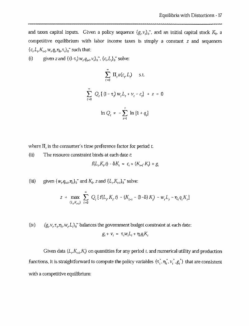
and taxes capital inputs. Given a policy sequence {goi,} 0-, and an initial capital stock K0, a

competitive equilibrium with labor income taxes is simply a constant z and sequences

fc,,Lt,K„,,,w„q„n„tja- such that:

(i) given z and f(1-t)w,,q„,,,v,W, fc,,L,1 0- solve:

E u (ce s.t.t=0

E Q [ (1 - Tr wt L t + v1 - ct] + z = 0t=0

In CZ - E ln [1 +

where H, is the consumer's time preference factor for period t.

(ii) The resource constraint binds at each date t

f(L,,Kr,t) - E)K, et + (K1, 1-K,) + g,

(iii) given {w„q,,,t00- and K0 , z and {L,K„)); solve:

z = max E Qt [ f(L r K,,t) - (K, ,} - (1 -8) Kt) - w,L t - ntqtK{.1.,1<m) t=0

(iv) fg,,v,,T,,n,,w,,LX- balances the government budget constraint at each date:

gt + v, = rliq,K,

Given data (L,,K+1,K) on quantities for any period t, and numerical utility and production

functions, it is straightforward to compute the policy variables (r t*, rl t*,vt*,gt*) that are consistent

with a competitive equilibrium:


uL (cr L i) fK(KrLrt) -T * 1 + - - 1

u c(c r fi(L r t)e

.rtt 11 (ct_,)

- 14ct)

= cr + [ - (1-45) Kt] - f(Lr, - T,* 1,1A,, Kr, 0

gr = f(L e Ke t) - cr - [K (1-6) IC]

where the term in square brackets is simply gross investment and It t is the consumer's date (t-1) one

period forward rate of time preference.

I use production and utility functions familiar from the real business cycle literature (eg.,

King, Plosser, and Rebelo 1988):1

u(c,L) E In c + 6 ln (1-L)

f(Lr, K r -----e A r L tia Ktl-P

where L is measured as manhours as a ratio of the annual "time endowment" (2500 hours per

person) for the population aged 15 and over, and all other quantities are measured per person aged

15+.

Appendix Table 1 reports {L,,c/11,} for t = 1929-50 (where If, is date t output)? Four

adjustments are made during wartime (1939-48) a to reflect the mismeasurement of output and the

involuntary nature of wartime military labor supply (not captured in the model above). First,

output is measured for the civilian sector only, under the assumption that civilian and military

personnel produce measured output in proportion to their measured labor income. To be consistent

`Mulligan (2000) studies two other functional forms as well, finding very similar resultsfor the Great Depression and somewhat different results for WWII and other time periods.

'Data sources, and the wartime adjustments below, are explained in Mulligan (2000).

'Results are quite insensitive to small changes in the definition of "war years" becausethese adjustments are trivial when the military is small, or there is a volunteer force.

(14)


with this adjustment, the second adjustment is to measure labor input as civilian manhours only.

Most wartime soldiers were drafted, so it is questionable whether their consumption and

leisure is as voluntary as modeled above. My third adjustment is therefore to calculate

consumption as civilian consumption expenditure per civilian aged 15-1-. 4 This adjustment slightly

increases measured wartime consumption.

IV. B. Simulated Policies

Given the numerical utility and production functions, the formulas for the policy variable

consistent with the model's competitive equilibrium are:

- 1 - L r 0 c,

(1-L) r3 f(L t, K e

The last column of Appendix Table 1 calculates {T;} for t= 1929-50, using parameters p = 0.615 and

0 = 0.7. 5 The dual approach does not have implications for transfers and government consumption

that can be tested with national accounts data because the national accounts calculate these to fit

the model (at least if we interpret purchases and sales of government debt as lump sum transfers

and taxes), so (14) ' neglects the equations simulating transfers and government consumption.

'Civilian consumption is measured as the difference between aggregate personalconsumption expenditures and one half of military wages (assuming that half of military wagesare saved, paid in taxes, or paid to civilian family members).

'These are basically those used in the literature, with small differences due to thedifferent time period studied, and my explicit modeling of distortionary taxes.

(14) '

•■■Wm* ••••.,

0.0


OA

0.3

e 0.2

-0.0 —

-0.1

1930 1935 1940 1945 1950year

tau*tau (Barro-Sahas + sales)

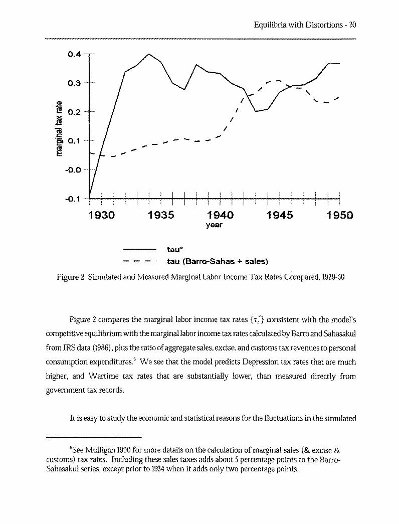
Figure 2 Simulated and Measured Marginal Labor Income Tax Rates Compared, 1929-50

Figure 2 compares the marginal labor income tax rates {t,*} consistent with the model's

competitive equilibrium with the marginal labor income tax rates calculated by Barro and Sahasakul

from IRS data (1986) , plus the ratio of aggregate sales, excise, and customs tax revenues to personal

consumption expenditures. 6 We see that the model predicts Depression tax rates that are much

higher, and Wartime tax rates that are substantially lower, than measured directly from

government tax records.

It is easy to study the economic and statistical reasons for the fluctuations in the simulated

6See Mulligan 1990 for more details on the calculation of marginal sales (& excise &customs) tax rates. Including these sales taxes adds about 5 percentage points to the Barro-Sahasakul series, except prior to 1934 when it adds only two percentage points.


marginal labor income tax rate {tit } . To understand the statistical reasons, recall from (14) ' that

it , up to the ratio 8/0 of constants, is one minus the product of the labor-leisure and consumption-

output ratios. Figure 3 displays the measured time series for those ratios, and we see how the

consumption-output ratio is pretty steady except during the war when it is a bit lower. So most

of the variation in t; comes from the labor-leisure ratio which is low in the depression and high in

the war, so that simulated marginal tax rates are high during the war and low during the

Depression. The basic patterns in the data are hardly controversial – see, for example, Friedman

(1957, p. 1171) on low-to-medium frequency constancy of the consumption-output ratio and Lucas

and Rapping (1969) labor fluctuations.


1,4

1.2

1

0 0.8I! 4. e a

0.6 %S ti, e♦i .—

0.4

0.2

0 H 11930 1935 1940 1945 1950

year

labor/leisure — MN, MIO I consumption/output

Figure 3 Components of Simulated Labor Tax Rates: By Data Source, 1929-50

I have not removed trends from the data, but we see from Figure 3 that trends are not

particularly noticeable in the data I use to simulate marginal tax rates. Perhaps this is one

advantage of the dual approach – there is less reason to remove trends of from the basic data

(because there is not much trend!) and we might worry less about the sensitivity of results to trend

estimation.

Figure 4 displays the economic components of the simulated tax rate, namely the marginal

product of labor and the marginal rate of substitution (see equation (14)). The marginal product

of labor, computed as 0.615 times the average product of labor, is displayed as a solid line. It follows

a pretty steady trend over time, except a bump during the war and no growth 1929-33.

Mao

ale


1930 1935 1940 1945 1950year

MRS - MPL

Figure 4 Components of Simulated Labor Tax Rates: By Economic Margin, 1929-50

For the most part, the simulated marginal rate of substitution (MRS), or marginal value of leisure

time, is less than the marginal product of labor (MPL). Perhaps surprising is the dramatic

divergence of MRS from MPL during the 1929-33 period (30 or 40 percentage points!) , a wedge

which persists until the war. As I discuss in the next subsection, the rapid emergence of this wedge,

and its persistence, are crucial for understanding the Great Depression.

IV. C. Understanding the Great Depression

Figure 2 and 4 make an important point — if an aggregative competitive equilibrium model

is to explain the Great Depression, at least with Cobb-Douglas production and utility functions,


it must explain why MRS and MPL diverged so dramatically 1929-33 and why the wedge persisted.

This point has implications for many theories explored in the literature:

IV.C.1. Productivity Shocks Cannot Explain 1929-33, or 1933-39

Cole and Ohanian (1999, p. 3) suggest that, if it could be argued that productivity shocks

({/0 in my notation) were large and persistent enough, then a real business cycle model could fit

the 1930's data pretty well. They reject this explanation because they see no reason why

productivity would have been low after 1933, but my analysis rejects it for a very different reason:

there is no productivity series {A t} that can be fed into the real business cycle model (without some

of the distortions mentioned below) to fit the Depression data because that model equates MRS

and MPL for any realization of the productivity series.

Similarly, Cole and Ohanian (1999, p. 3) and Prescott (1999, p. 26) suggest that the period

1929-33 is not puzzling for the real business cycle approach, because there are lots of candidates for

productivity shocks during that period. Perhaps there are good candidates, but productivity shocks

do not cause MRS and MPL to diverge in the real business cycle model – and my Figures 2 and 4

shows that such divergence is what happened 1929-33. 7 In summary, in addition to (or instead of?)

the right time series for productivity shocks, the real business cycle model needs to be amended to

explain why MRS and MPL diverged and why that wedge persisted.

IV.C.2. Personal Income Taxes are not an Important Part of the Labor-Leisure Distortion

Cole and Ghanian (1999, p. 6) suggest that government purchases, or taxes on factor

incomes, might help explain some of the Depression economy. However, my analysis suggests that

government purchases, and taxes on capital, cannot explain why MRS and MPL would be

differernt, let along why and how that wedge would persist over time. Of course, taxes on labor

income create such a wedge, but Barro and Sahasakul's study suggests that federal taxes on payroll

and individual income were trivial, and unchanging, during the period. Indeed, IRS records (IRS,

various issues) show that the vast majority of the population did not file individual income tax

returns during the 1930's, so that any IRS-induced tax wedge affected very few people (not to

'To put it another way, an adverse productivity shock decreases the MRS and MPLtogether in the real business cycle model.


mention small for the few affected).

Taxes on consumption expenditure are also expected to drive a wedge between MRS and

MPL. The federal government did not have a general sales tax, although it does have (and has had)

excise taxes on goods such as cigarettes, gasoline, and imports. More general sales taxes have been

collected by states and localities. However, the revenues from these taxes are too few, and not

changing enough over time, to drive much a of wedge. Hence, we see a dashed line in Figure 2,

which is the combined marginal tax rate from sales, excise, customs, and federal labor income taxes,

that is close to zero and not increasing much until WWII.

IV.C.3. How Much Can International Trade Explain?

The Great Depression was an important time in the history of international trade, with

dramatic increases in tariff rates as a result of the Hawley-Smoot Act, other legislation, and other

nonlegislation (see, for example, Taussig 1931 or Crucini 1994). Some (eg., Metlzer 1976, Crucini

and Kahn 1994) have suggested that international trade was an important influence on aggregate

activity during that period. A key question is: would changes in tariffs drive a large wedge between

MRS and MPL, and would that wedge persist for a decade?

The question is easily answered, in the negative, using Crucini and Kahn's (1994) dynamic

general equilibrium trade model. Theirs is a two country model, with a representative agent in each

country. That agent consumes three types of goods (home nontraded, home traded, and foreign

traded) , and supplies his time to each of three sectors (traded consumption, untraded consumption,

and traded production materials). Crucini and Kahn do not have labor income taxes, so their model

implies an equation of the marginal value of time (in utility) with the marginal net-of-tariff revenue

product of labor (in production, in each of the three sectors). Of course, if their model did have

labor income taxes, the marginal labor income tax rate would be the wedge between the marginal

value of time and the marginal net-of-tariff revenue product of labor, computed in much the same

way as in the examples above:

uL(c1 , L)'E t = 1 +

ue (cr L) fL (Le Kr t)


There are two differences between (@) and the analogue for the neoclassical one-sector growth

model: (1) consumption is a composite good (eg., a CES aggregate of the three consumption goods

as in Crucini and Kahn's numerical model), and (2) IL is the equilibrium marginal revenue product

of labor, net of tariffs, in either the traded or untraded sectors. But, because Crucini and Kahn (1994,

pp. 439, 441) assume production is Cobb-Douglas in labor in both sectors - with the same labor

share - my calculations ((14) ' , repeated below for convenience) for the neoclassical growth model

can be applied to Crucini and Kahn's model with one very minor correction.

= I - L e

(1-L) p f(L 0

The relevant marginal product of labor is net of tariffs, so it is computed as labor's share times

GNP net of tariff revenue - not total GDP - per unit labor input.' However, the sign and magnitude

of this correction depends on the sign and magnitude of (net factor income from abroad minus tariff

revenue and) share of GDP. According to the Bureau of Economic Analysis (1999) , net factor

income from abroad was positive in the 1930's, and between 0.4 and 0.8 percent of GDP. Crucini

and Kahn (1998, p. 443) suggest that tariff revenues was on the order of 0.7 percent of GDP, so the

difference between the two is essentially zero. In other words, the simulated tax wedge is

essentially numerically identical for the neoclassical growth and Crucini-Kahn models, even though

those models suggest that somewhat different ingredients go into the calculation of the marginal

'To derive this from Crucini and Kahn's (1996) equations, first compute aggregate laborincome (wL in my notation) by adding the three marginal revenue product of labor equationsfrom their p. 460, weighting by labor income and using the Cobb-Douglas functional forms(with identical labor shares for each sector). Part of this sum is aggregate expenditure onintermediate inputs (see their fifth-to-last equation on p. 460) , which in turn is tariff revenueplus the compensation for those selling materials to that constant returns sector (to see this, addthe two p. 460 intermediate marginal revenue product equations). Simple subtraction thenimplies that aggregate labor income (wL in my notation) is labor share times GNP minus tariffrevenue. In other words, the marginal revenue product of labor w is GNP minus tariff revenue,times labor share, and divided by aggregate labor input L.

(14) '


revenue product of labor.'

Hence, Crucini and Kahn's (1996, p. 446) explanation of Depression labor supply is grossly

inconsistent with Cobb-Douglas functional forms and three basic time series - output, consumption

expenditure, and aggregate hours - used in my Figure 3, in the business cycle literature, and by

Crucini and Kahn themselves. Their model "explains" Depression labor supply by simulating a

counterfactually low average product of labor, rather than driving an important wedge between the

marginal value of time and the marginal product of labor. The only hope for a trade model like

Crucini and Kahn's to explain such a large wedge is for tariff revenue to be a large share of GDP,

and larger than the share of net factor income from abroad.' In this sense, Crucini and Kahn's

analysis supports, rather than refutes, Lucas's (1994) claim that "the effects of fa tariff] policy (in

an economy with a five percent foreign trade sector...) would be trivial."

IV. C.4. Labor Market Regulations

Prescott (1999, p. 26) suggests that labor market regulations may have hurt employment

during the Depression. My Figure 2 can guide future studies of this hypothesis. In particular, were

there regulations driving a wedge between MRS and MPL? Did those regulations first appear, or

take effect, 1929-33? How big was the wedge - as large as 30 or 40 percent?

On the first point, it should be noted that labor market regulations are varied. Some may

have no effect because the regulations require workers and employers to do things that they would

already do, or because the regulations are not enforced. Others may lower the marginal product

'I have measured c as real consumption expenditures. In principle a price index could bedesigned based on Crucini and Kahn's utility function so that changes over time in realconsumption expenditures would be the same as changes over time in the quantity of thecomposite consumption good. In practice (ie, using the GDP deflator or the Consumer PriceIndex), the real consumption expenditures may either over- or under-state compositeconsumption, because of imperfections in the price index, and a second adjustment of (14)' maybe required. However, we see from (14) ' and our empirical results how, in order to explain theDepression gap between MRS and MPL, any adjustment to real consumption expendituresmust (a) increase measured real consumption during the Great Depression, and (b) be largeenough to drive a 30% wedge.

'Or for exported goods to be extremely labor intensive - a possible that was notexplored by Crucini and Kahn and probably not quantitatively interesting.


of labor schedule (or raise it?) , perhaps by restricting (or helping?) firms from using the most

efficient production process. But of particular interest for my study are regulations that drive a

wedge between MRS and MPL. According to the textbook analysis, a binding minimum wage is

one example because it puts some people out of work - a movement down the aggregate labor

supply schedule - and moves employers up their MPL schedule (aka, labor demand curve) .

Mandatory fringe benefits, if they are valued by employees at less than their cost to employers,"

also drive such a wedge.

It is hard to identify which regulations drive a wedge between MRS and MPL, let alone

accurately quantify the wedge created by the large and varied portfolio of federal regulation.

However, recall from Figure 2 that the changes in implied tax rates to be explained are quite large

- on the order of 30 percentage points or more for the entire labor force. Hence, even a rough

qualitative analysis of federal labor regulation can reveal whether labor market regulation and its

changes over time are a viable explanation. Mulligan (2000) attempts such a qualitative analysis,

and his results are summarized here.

First, notice that, according to the Center for the Study of American Business' 1981

Directory of Federal Regulatory Agencies, the only federal labor regulations begun in the 1930's and

covering more than a few workers were the 1935 Wagner Act and the 1938 Fair Labor Standards Act

(FLSA). I consider the effect of unions below, so that leaves the 1938 Fair Labor Standards Act

(ELSA) which was at least five years after the large wedge appears in Figure 2.

Second, labor regulation that was at least as comprehensive of FLSA appeared in the 1960's

and 1970's (including in this later regulatory explosion, for example, was the 1970 Occupational

Safety and Health Act), but we see nothing like the Great Depression in the 1960's or 1970's and,

according to Mulligan (2000), nothing like the 1930's divergence of MRS and MPL.

IV C 5 Can Monopoly Unions be Part of the Story?

Monopoly unions, by definition, deliberately drive a wedge between MRS and MPL in order to

raise member incomes. The size of this wedge is related to the "relative union wage gap", the

percentage gap between a typical union worker and an observably otherwise similar nonunion

"ie, the mandated benefits exceed the amount workers would demand in the absence ofregulation. See, for example, Summers (1989) for some analysis of this point.


worker, often measured in the labor economics literature. My approach is to use the estimates

from that literature to quantify the potential contribution of monopoly unionism to the gap

between MRS and MPL as measured in the aggregate.

Lewis (1963, 1986) surveys much of a large literature attempting to estimate the union wage

gap for various industries. He stresses (1986, pp. 9, 187) that wage gaps vary a lot from industry

to industry, and are typically overestimated because union workers are expected to have more

unmeasured human capital than nonunion workers (so that measured wage gaps are only part

monopoly union power, and part human capital differences). With these caveats in mind, I

construct Table 1 below by reproducing and extending Lewis' (1963) Table 50, reporting by time

period the relative wage gap for the "typical" unionized worker.

Table 1: Union Relative Wage Gaps by Time Period

parameter values

time period lower estimate upper estimate

1923-29 0.15 0.20

1931-33 0.25

1939-41 0.10 0.20

1945-49 0 0.05

1957-58 0.10 0.15

1967-70 0.12 0.16

1971-79 0.13 0.19

Table lists the difference between the typical union wage and the nonunion wage of

observationally similar workers, as a fraction of the nonunion wage.

Source: Lewis (1963, Table 50 and 1986, p. 9)

Notice in particular that the union wage gap is about twice as large during the Great Depression

(see also Lewis 1963, pp. 40.

The measured wage gap need not be exactly the percentage wedge between MRS and MPL


in the union sector. But it is perhaps a reasonable first estimate of that wedge - and would be

identical to the wedge in the case that the wedge is zero in the nonunion sector, and the value of

time (MRS) is the same in both sectors. 0 With this, and Lewis' (1986, p. 9) overestimation caveat,

in mind I use the "lower" wage gaps reported in Table 1 as estimates of the MRS/ MPL wedges in

the union sector.

My calculations of implied tax wedges are for the entire economy, and not just the union

sector, How much can monopoly unionism affect the average tax wedge? Assuming the monopoly

union wedge is zero for nonunion workers, the size of the monopoly union wedge for the average

worker is the product of the union wedge and union density (ie, the fraction of the labor force that

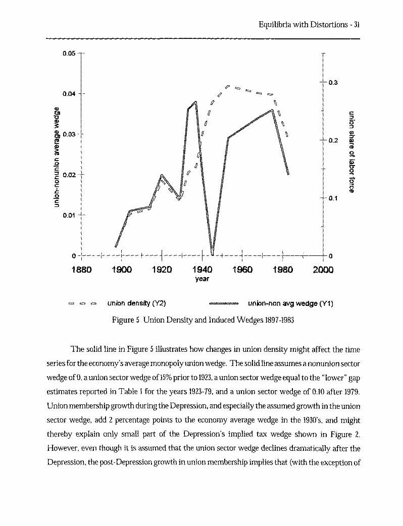
is unionized). Using Rees' (1989 Table 1) 13 time series, we see from the dashed line in Figure ? that

union density increased somewhat during the 1930's - reaching 18% - while the largest increases

during the century were after the Depression. Union density has declined since the 1950's (see also

Freeman and Medoff 1984, Figure 15-1) , and perhaps that decline accelerated in the late 1970's and

1980's.

'The wedge is one minus the ratio of union sector MPL to union sector MRS which,under these assumptions, is the same as one minus the ratio of union sector wage to unionsector MRS, which equals one minus the ratio of union sector wage to nonunion sector MRS,which is the same as one minus the ratio of union sector wage to nonunion sector wage.

'I use Census Bureau (1975, series D-17, 1900 value) to fill in Rees' missingnonagricultural employment for the year 1897, and then Census Bureau (1975) series D-167, 170and BLS series LFU40000000, LFU11102000000 to convert Rees' ratio to nonagriculturalemployment to a ratio to the entire labor force.

— 0.30.04 —

a.)

a,d) 0.03 m

a

2 0.02 —0

00Cn

D.01 —

0.2

0.1


0.05 —

1880 1900 1920 1940

1960 1980 2000year

St, 0 0 union density (Y2) ======= union-non avg wedge (Y1)

Figure 5 Union Density and Induced Wedges 1897-1983

The solid line in Figure 5 illustrates how changes in union density might affect the time

series for the economy's average monopoly union wedge. The solid line assumes a nonunion sector

wedge of 0, a union sector wedge of 15% prior to 1923, a union sector wedge equal to the "lower" gap

estimates reported in Table 1 for the years 1923-79, and a union sector wedge of 0.10 after 1979.

Union membership growth during the Depression, and especially the assumed growth in the union

sector wedge, add 2 percentage points to the economy average wedge in the 1930's, and might

thereby explain only small part of the Depression's implied tax wedge shown in Figure 2.

However, even though it is assumed that the union sector wedge declines dramatically after the

Depression, the post-Depression growth in union membership implies that (with the exception of


the war) the economy-average wedge is pretty stable until the 1980's.

In other words, even if the union wage effect appeared for the first time in the 1930's,

monopoly unionism cannot explain a wedge of more than 4%, so most wedge shown in Figure 2 is

unexplained.

IV.C.6. What about Monetary Shocks?

Whether monetary shocks can explain what is shown in Figures 2-4 depends on the margins

distorted by those shocks. If monetary shocks have there primary effect on credit markets or

otherwise distort intertemporal margins (as they do in Lucas 1975 and some other island models) ,

then they cannot explain Figures 2-4. Barro and King (1984) emphasize that changes in

intertemporal margins cause consumption and leisure to move together or, in terms of Figure 4,

cause the MRS and MPL to move together.

In Lucas-island models of the confusion of real and nominal magnitudes, MRS is still

equated to MPL (monetary shocks instead create a gap between perceived and actual intertemporal

marginal rates of transformation) and thus inconsistent with Figure 4. But perhaps a modified

monetary confusion model would predict that MRS is equated to perceived MPL, which we might

expect to be less than the actual MPL shown in Figure 4 during those periods when the price level

is less than expected. But could the misperception be as large as 30 or 40 percent and could it

persist for a decade?

Sticky nominal wages, perhaps as modeled Barro and Grossman (1971) might well drive a

wedge between MRS and MPL in response to monetary shocks. However, the timing and

magnitude of such rigidities are difficult to measure independently of the average product and

consumption series shown in Figure 4. This sets the "rigid wage" hypothesis apart from the public

finance distortions (whose magnitude and timing were independently measured using IRS tax rules

and return data) and the monopoly union distortions (whose magnitude and timing were

independently measured using union density and Lewis's comparisons of union and nonunion

sectors). Are there direct measures of wage rigidity for the 1930's? Or are there "flexible wage"

sectors that could be compared with "rigid wage" sectors?

According to one special case of the "rigid wage" hypothesis (and one suggested by Lewis,

eg., 1963 pp. 50 , wages are rigid only in the union sector, in which case wage rigidity can be


measured independently of average productivity by comparing wages in union and nonunion

sectors. This is what Lewis does, and his results are transformed into a wedge between MRS and

MPL in the previous section. In other words, rigid wages may only be another interpretation of the

calculations I interpreted above as "monopoly union."

IV.D. Intertemporal Distortions During the Period

The procedure shown in Section III can also be used to simulate corporate profits tax rates

for the real business cycle model. The formula is (repeated from (14) for the reader's convenience):

TK(KrEc t) - 8 n t - - 1

e u itch]) —1

i(c)

where it, is the consumer's date (t-1) one period forward rate of time preference. With the Cobb-

Douglas production and utility functions, the consumer's ratio of marginal utilities is just

consumption growth, and the marginal product of capital is proportional to the output-capital ratio.

li t and its two components are graphed in Figure 5.

1 1 1 H

1930 1935 19451940 1950


year

...... eta* (yi)– - MI I IMRS-(1-delta) (Y2)

...... MPK (Y2)

Figure 6 Simulated Marginal Tax Rates and Their Components, 1929-50

Figure 5 shows how the marginal product of capital (MPK, shown as a solid blue line)

declined slightly 1929-33, and then increased steadily until the end of the war. Consumers'

intertemporal marginal rate of substitution (IMRS, shown as a dashed blue line) followed the same

pattern but was less regular from year-to-year. Hence, the average simulated capital income tax

rate was zero. Perhaps the IMRS was persistently below MPK early in the Depression, and

persistently higher later, so it might be said that the model predicts heavy capital taxation early, and

capital subsidies later in the Depression.

V. Conclusions

Rather than using a numerical model of private behavior and measured government policies


to simulate quantities and prices for comparison with measured quantities and prices (the "primal"

approach for empirically evaluating competitive equilibrium models), I suggest that it is easier and

economically more informative to use a numerical model of private behavior and measured

quantities to simulate prices and government policies for comparison with measured prices and

policies (the "dual" approach for empirically evaluating competitive equilibrium models). The dual

approach, which does nothing more than compute wedges between measured marginal rates of

substitution and transformation, is easily applicable to competitive equilibrium models with many

(even infinite) time periods, many heterogeneous agents, many sectors, and many government

policy instruments.

V.A. Understanding the American Economy 1929-50

I illustrate the method by evaluating the performance of the neoclassical growth model for

the 1929-50 American economy. Assuming that the real business cycle model is not far off with

Cobb Douglas utility and production functions, the data show how the marginal product of labor

(MPL) diverged from the marginal value of time (MRS) by 30-40 percent from 1929-33, and that

wedge persisted until WWII, when the wedge between MPL and MRS was more than 20

percentage points smaller than it was in the early 1930's. This is particularly puzzling in light of

federal tax policy during the period, where marginal labor income tax rates were practically zero

during the 1930's and at their height during the war.

I also show how the tax wedge can be used to organize and evaluate existing and potential

theories of the Great Depression. Whether the theory be one of productivity shocks, monetary

shocks, factor income taxes, labor market regulation, or monopoly unionism, does the theory

predict a wedge between MRS and MPL? If so, when should the wedge first appear? Can the

wedge be as large as 30 or 40 percent?

As I have applied it, the dual approach attributes to restraints of trade any failure of the

observed determinants of marginal rates of transformation and marginal rates of substitution to

move together, and compares those failures (ie, simulated "tax wedges") to measures of restraints

of trade such as regulation, distortionary taxes, and monopoly unionism. Another logical


possibility is that preferences are shifting over time in ways that cannot be directly measured.w

Because apparent gaps between marginal rates of substitution and transformation might be

attributed to either preference shifts or restraints of trade, the dual approach is best applied to

competitive equilibrium models for which all of the major determinants of preferences are

observed.

V.B. Lessons for Other Applications

My evaluation of the real business cycle model with data from 1929-50 highlights several

advantages of the dual approach to the empirical evaluation of dynamic competitive equilibrium

models. The first is the simplicity of the calculation: I simulate marginal labor income tax rates

merely by multiplying the ratio of labor to leisure by the consumption-output ratio. One

byproduct of this simplicity is that there is no need for the approximations often found in the

literature – such as discretizing the state space, restricting policy functions to be in the space of low

order polynomials, or assuming that capital begins the time period in its "steady state". Second,

the model can be partially evaluated even with very limited data. Although the neoclassical growth

model is an infinite period model, with capital and time-specific production possibilities, I made

labor distortion calculations based only on 22 years of the labor-leisure and consumption-output

ratios – without data on capital or "productivity." Informative calculations could have been made

with even fewer years of data. Third, even with infinite data, the dual approach partitions

complicated models into simpler pieces.5 In the case of the real business cycle model, I show how,

assuming Cobb-Douglas utility and production, the Great Depression was a time of departure

between the marginal product of labor and the marginal value of time – my argument does not

depend on whether there are multiple capital goods, or whether there are adjustment costs to

investment, or on other assumptions of the real business cycle model. Fourth, although interpreting

"This is the approach of Hall (1997) who, in his study of postwar business cycles,assumes that there are no wedges created by restraints of trade – so that preference shifts arethe only reason observed determinants of marginal rates of transformation and marginal ratesof substitution might fail to move together.

' sit does so without approximation, other than those embodied in any numerical model ofprivate behavior.


long run trends in the data have received a lot of attention in the business cycle literature, the dual

approach is robust to a number of possible interpretations of those trends. In particular, if those

trends do not affect the ratio of labor to leisure, or affect the ratio of consumption to output, then

they do not affect my simulated labor income tax rates.

V.C. Forecasting vs. Empirical Evaluation

My dual approach uses measured quantities as input and is therefore not directly applicable

to forecasting the quantity and price effects of a hypothetical government policy - an important

exercise in policy research. However, the dual approach is best for empirically evaluating a

competitive equilibrium model, and hence a prerequisite for predicting the effects of a hypothetical

government policy - at least for those who only forecast with models shown to have some empirical

success.

VI. Appendix: Data and Calculations for the period 1929-50


Appendix Table 1: 1929-50 data and Labor Distortion Calculations

year civilian labor military consumption/ simulated marginal laborlabor outputs income tax rates

t L. 1,, 0.7 ct

t t = 1 -c/Y,(1-L 1) 0.615 Yt

1929 0.560 0.002 0.747 -0.0941930 0.515 0.002 0.769 0.0621931 0.468 0.002 0.792 0.1991932 0.412 0.002 0.828 0.3351933 0.407 0.002 0.814 0.3581934 0.402 0.002 0.780 0.3971935 0.419 0.002 0.763 0.3691936 0.452 0.002 0.743 0.2961937 0.466 0.002 0.727 0.2721938 0.428 0.002 0.746 0.3591939 0.442 0.002 0.734 0.3371940 0.452 0.004 0.707 0.3321941 0.482 0.013 0.648 0.2971942 0.510 0.034 0.566 0.2801943 0.525 0.082 0.526 0.2011944 0.512 0.102 0.524 0.2091945 0.479 0.091 0.578 0.2691946 0.472 0.023 0.668 0.2901947 0.475 0.011 0.674 0.2931948 0.473 0.010 0,659 0.3151949 0.450 0.010 0.668 0.3511950 0.454 0.011 0.655 0.352

Source: Kendrick Kendrick BEA NIPA

1 1939-48 for the civilian sector only% Leisure time = I - civilian and military labor. Labor input = civilian & military labor,except during wartime (1939-48)

VII. References

Aiyagari, S. Rao, Lawrence J. Christiano, Martin Eichenbaum. "The Output, Employment, and


Interest Rate Effects of Government Consumption. Journal of Monetary Economics. 30(1),

October 1992: 73-86.

Barro, Robert J. and Herschel I. Grossman. "A General Disequilibrium Model of Income and

Employment." American Economic Review. 61(1), March 1971: 82-93.

Barro, Robert J. and Robert G. King. "Time-separable Preferences and Intertemporal-Substitution

Models of Business Cycles." Quarterly Journal of Economics. 99(4), November 1984: 817-39.

Baxter, Marianne and Robert G. King. "Fiscal Policy in General Equilibrium." American Economic

Review. 83(3) , June 1993: 315-34.

Braun, R. Anton and Ellen R. McGrattan. "The Macroeconomics of War and Peace." in Olivier

Jean Blanchard and Stanley Fischer, eds. NBER Macroeconomics Annual 1993. Cambridge and

London: MIT Press, 1993: 197-247.

Burnside, Craig, Martin Eichenbaum, and Jonas D.M. Fisher. "Assessing the Effects of Fiscal

Shocks." NBER Working paper #7459, January 2000.

Cole, Harold L. and Lee E. Ohanian. "The Great Depression in the United States from a

Neoclassical Perspective." Federal Reserve Bank of Minneapolis Quarterly Review. 23(1),

Winter 1999: 2-24.

Crucini, Mario J. "Sources of Variation in Real Tariff Rates: The United States, 1900-1940."

American Economic Review. 84 (3) , June 1994: 732-43.

Crucini, Mario J. and James Kahn. "Tariffs and Aggregate Economic Activity: Lessons from the

Great Depression." Journal of Monetary Economics. 38 (3) , December 1996: 427-67.

Friedman, Milton. A Theory of the Consumption Function. Princeton, NJ: Princeton University

Press, 1957.

Hall, Robert E. "Macroeconomic Fluctuations and the Allocation of Time." Journal of Labor

Economics. 15(1), Part 2 January 1997: S223-50.

Hansen, Lars Peter and Thomas J. Sargent. Recursive Linear Models of Dynamic Economies.

Manuscript, University of Chicago, January 1991.

Houthakker, Hendrik S. "The Pareto Distribution and the Cobb-Douglas Production Function

in Activity Analysis." Review of Economic Studies. 23, 1955: 27-31.

Hummels, David. "Toward a Geography of Trade Costs." Working paper, University of

Chicago, January 1999.


Kendrick, John W. Productivity Trends in the United States. Princeton: Princeton University Press,

1961.

King, Robert G., Charles I. Plosser and Sergio T. Rebelo. "Production, Growth and Business

Cycles: I. The Basic Neoclassical Model." Journal of Monetary Economics. 21(2) , March

1988: 195-232.

Kydland, Finn and Edward C. Prescott. "Time to Build and Aggregate Fluctuations." Econometrica.

50 (6), November 1982: 1345-70.

Lucas, Robert E., Jr. "Review of Milton Friedman and Anna J. Schwartz's 'A Monetary History

of the United States, 1867-1960. — Journal of Monetary Economics. 34 (1) , August 1994: 5-16.

Lucas, Robert E., Jr. and Leonard A. Rapping. "Real Wages, Employment, and Inflation." Journal

of Political Economy. 77 (5) , September 1969.

Lucas, Robert E., Jr. and Leonard A. Rapping. "Unemployment in the Great Depression: Is There

a Full Explanation?" Journal of Political Economy. 80(1), January 1972:186-91.

Meltzer, Alan. "Monetary and Other Explanations of the Start of the Great Depression." Journal

of Monetary Economics. 2(4) , November 1976: 455-71.

Mulligan, Casey B. "Pecuniary Incentives to Work in the United States during World War II."

Journal of Political Economy. 106 (5) , October 1998: 1033-77.

Mulligan, Casey B. "Microfoundations and Macro Implications of Indivisible Labor." NBER

working paper #7116, May 1999.

Mulligan, Casey B. "A Century of Labor-Leisure Distortions." Manuscript, University of

Chicago, September 2000.

Ohanian, Lee E. "The Macroeconomic Effects of War Finance in the United States: World War

II and the Korean War." American Economic Review. 870), March 1997: 23-40.

Prescott, Edward C. "Theory Ahead of Business Cycle Measurement." Federal Reserve Bank of

Minneapolis Quarterly Review. 10, Fall 1986: 9-22.

Prescott, Edward C. "Some Observations on the Great Depression." Federal Reserve Bank of

Minneapolis Quarterly Review. 23 (1) , Winter 1999: 25-31.

Rees, Albert. The Economics of Trade Unions. Chicago: University of Chicago Press, 1989.

Taussig, Frank W. The Tariff History of the United States. New York: G.P. Putnam's and Sons,

1931.


United States, Bureau of Economic Analysis. Survey of Current Business. November 1999. [data

also available at www.bea.doc.gov/bea/dnl.htm}

United States Department of the Treasury, Internal Revenue Service. Statistics of Income, various

issues.

Wu, Yangru and Junxi Zhang. "Endogenous Markups and the Effects of Income Taxation:

Theory and Evidence from OECD Countries." Journal of Public Economics. 77 (3) ,

September 2000: 383-406.

a dual method of empirically evaluating dynamic

Documents