a dynamic f5 algorithm
TRANSCRIPT
The University of Southern Mississippi The University of Southern Mississippi
The Aquila Digital Community The Aquila Digital Community
Dissertations
Spring 2020
A Dynamic F5 Algorithm A Dynamic F5 Algorithm
Candice Mitchell
Follow this and additional works at: https://aquila.usm.edu/dissertations
Part of the Algebra Commons
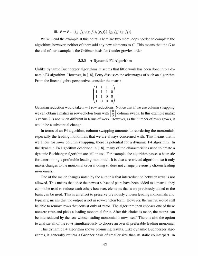
Recommended Citation Recommended Citation Mitchell, Candice, "A Dynamic F5 Algorithm" (2020). Dissertations. 1748. https://aquila.usm.edu/dissertations/1748
This Dissertation is brought to you for free and open access by The Aquila Digital Community. It has been accepted for inclusion in Dissertations by an authorized administrator of The Aquila Digital Community. For more information, please contact [email protected].
A DYNAMIC F5 ALGORITHM
by
Candice Bardwell Mitchell
A DissertationSubmitted to the Graduate School,the College of Arts and Sciences
and the School of Mathematics and Natural Sciencesof The University of Southern Mississippiin Partial Fulfillment of the Requirements
for the Degree of Doctor of Philosophy
Approved by:
Dr. John Perry, Committee ChairDr. Bernd Schröder
Dr. Karen KohlDr. Jiu Ding
Dr. Rajeev Agrawal
Dr. John Perry Dr. Bernd Schröder Dr. Karen S. CoatsCommittee Chair Director of School Dean of the Graduate School
May 2020

COPYRIGHT BY
CANDICE BARDWELL MITCHELL
2020
ABSTRACT
Gröbner bases are a “nice” representation for nonlinear systems of polynomials, where by
“nice” we mean they have good computation properties. They have many useful applications,
including decidability (whether the system has a solution or not), ideal membership (whether
a given polynomial is in the system or not), and cryptography. Traditional Gröbner basis
algorithms require as input an ideal and an admissible term ordering. They then determine a
Gröbner basis with respect to the given ordering. Some term orderings lead to a smaller basis,
but finding them traditionally requires testing many orderings and hoping for better results.
A dynamic algorithm requires as input only the ideal and allows the term ordering to vary at
each step of the algorithm. Previous work has shown that this often produces a smaller basis
and/or finds a basis in a shorter time frame. Since some Gröbner bases under certain term
orderings are extremely large, it is advantageous to find ways to compute smaller bases. The
F5 algorithm is a traditional algorithm that computes a Gröbner basis in a way that attempts
to avoid computing S-polynomials that reduce to zero. Since S-polynomials that reduce to
zero do not add any useful information, avoiding these computations can drastically reduce
the amount of work done. This work describes a dynamic F5 algorithm to compute Gröbner
bases. The algorithm combines the advantages of a traditional F5 algorithm by avoiding
the majority of S-polynomials that reduce to zero as well as the decrease in size that can be
gained using a dynamic algorithm.
ii
ACKNOWLEDGEMENTS
There are many who helped me to this point and so many different ways that they helped.
I am grateful to the Department of Mathematics at the University of Southern Mississippi for
allowing me to be a graduate assistant throughout my time here. I would not have been able
to pursue, much less complete, a PhD without the generosity of the Mississippi Space Grant
Consortium (MSSGC) Graduate Fellowship Program. I also want to thank my committee
for sticking with me through this process and their helpful guidance along the way.
I am extremely thankful for my advisor, John Perry. He sets high expectations but gives
me the tools I need to meet them. Dr. Perry has given me guidance and encouragement
when I needed it and left me to my own devices when it was necessary for my growth. He
has freely given his so much of his time and wisdom that I could never repay him.
My parents have supported me even though I squandered opportunities in my past. I
thank them for not only continuing to believe in me but also for all their help and support
with my family. My husband, Ben, has probably endured the most torture during this process.
He has somehow continued to be loving and supportive, and I will be in his debt for many
years to come. Finally, I am grateful for my boys, without whom I would have never pursued
this path: No matter how far you fall, you can still get up and reach for the stars. I love you
to the moon . . . and back!
iii
TABLE OF CONTENTS
ABSTRACT . . . . . . . . . . . . . . . . . . . . . . . . . . . . . . . . . . ii
ACKNOWLEDGMENTS . . . . . . . . . . . . . . . . . . . . . . . . . . . . iii
LIST OF ILLUSTRATIONS . . . . . . . . . . . . . . . . . . . . . . . . . . vi
LIST OF TABLES . . . . . . . . . . . . . . . . . . . . . . . . . . . . . . vii
LIST OF ABBREVIATIONS . . . . . . . . . . . . . . . . . . . . . . . . . viii
NOTATION AND GLOSSARY . . . . . . . . . . . . . . . . . . . . . . . . . x
1 Gröbner Bases . . . . . . . . . . . . . . . . . . . . . . . . . . . . . . . 11.1 Background 11.2 Monomial Orderings 41.3 Gröbner Basis Computation 9
2 Leading Monomials . . . . . . . . . . . . . . . . . . . . . . . . . . . . . 172.1 Introduction 172.2 Weighted Monomial Ordering 182.3 Background 202.4 Result 22
3 Dynamic Gröbner Basis Computation . . . . . . . . . . . . . . . . . . . 303.1 Introduction 303.2 Dynamic Buchberger Algorithms 333.3 A Dynamic F4 Algorithm 40
4 F5 Algorithm . . . . . . . . . . . . . . . . . . . . . . . . . . . . . . . . 474.1 Background 474.2 F5 Algorithm 51
5 Dynamic F5 Algorithm . . . . . . . . . . . . . . . . . . . . . . . . . . . 615.1 Introduction 615.2 Dynamic F5 Algorithm 615.3 Results 68
iv
5.4 Future Work 73
APPENDIX
A SOURCE CODE . . . . . . . . . . . . . . . . . . . . . . . . . . . . . . 75
B POLYNOMIAL SYSTEMS . . . . . . . . . . . . . . . . . . . . . . . . . 90B.1 Cyclic-4 90B.2 Cyclic-5 90B.3 Cyclic-6 91B.4 Cyclic-7 91B.5 Eco5 92B.6 Eco5(h) 92B.7 Eco6 92B.8 Eco6(h) 93B.9 Eco8 93B.10 Eco8(h) 93B.11 Katsura-5 94B.12 Noon3 94B.13 Noon4 94B.14 Noon4(h) 94B.15 Noon5 95B.16 Trinks 95
BIBLIOGRAPHY . . . . . . . . . . . . . . . . . . . . . . . . . . . . . . . 96
v
LIST OF ILLUSTRATIONS
Figure
2.1 Monomial diagrams illustrating which incompatible monomials u are detectableby DC and EDC. . . . . . . . . . . . . . . . . . . . . . . . . . . . . . . . . . 25
3.1 Monomial diagrams illustrating the Hilbert function for 〈x3,x2y〉 (a) and 〈x3,y3〉(b). . . . . . . . . . . . . . . . . . . . . . . . . . . . . . . . . . . . . . . . . 32
vi
LIST OF TABLES
Table
2.1 Number of incompatible monomials detected when testing Algorithm 3 be-fore the boundary vector criterion (“precheck”) in a dynamic F4 algorithm tocompute Gröbner bases. . . . . . . . . . . . . . . . . . . . . . . . . . . . . . 29
5.1 Number of S-polynomials computed using Buchberger’s algorithm (Buch), adynamic Buchberger algorithm (dynB) [19], the F5 algorithm, and the dynamicF5 algorithm (DynF5) described here. . . . . . . . . . . . . . . . . . . . . . . 69
5.2 Number of useless S-reductions to zero computed using Buchberger’s algorithm(Buch), a dynamic Buchberger algorithm (dynB) [19], the F5 algorithm, andthe dynamic F5 algorithm (DynF5) described here. . . . . . . . . . . . . . . . 71
5.3 Size of the Gröbner basis computing using Buchberger’s algorithm (Buch), adynamic Buchberger algorithm (dynB) [19], the F5 algorithm, and the dynamicF5 algorithm (DynF5) described here. . . . . . . . . . . . . . . . . . . . . . . 72
5.4 Computational time using the traditional F5 algorithm and the dynamic F5algorithm (DynF5) described here. . . . . . . . . . . . . . . . . . . . . . . . . 74
vii

LIST OF ABBREVIATIONS
DC - Divisibility CriterionEDC - Extended Divisibility Criterion
gcd - Greatest Common DivisorLC - Leading Coefficientlcm - Least Common MultipleLM - Leading MonomialLT - Leading TermM - the set of monomials in x1, . . . ,xn
Supp - Supporttp - LM(p)
tp,q - lcm(tp, tq)
viii
NOTATION AND GLOSSARY
General Usage and Terminology
For notation, we generally follow the example set in [5]. Unfortunately, there is little inthe way of a “standard” notation in Computational Algebra. We will use angle brackets,〈·〉 to represent ideals, but many authors have used parenthesis (·) to represent them. Weuse |·| to represent the sum of a vector’s elements as well as to represent a set’s cardinality.As usual, Z represents the integers. We will use Z≥0 to represent the nonnegative integers.As is typical, /0 represents the empty set. Capital letters are used to represent ideals andbases while lowercase letters are used as much as possible to represent fields and basiselements; however, neither are used exclusively for those purposes. When a notation may beunfamiliar to the reader, we define what it is intended to represent.
Algebra Basics
Definition 0.0.1 (Definition 1 of §1.2 in [5]). A monomial in x1, . . . ,xn is a product of theform n
∏i=1
xαii
where αi ∈ Z≥0, the set of nonnegative integers.
For simplicity, we can represent monomials in the following way. Let α = (α1, . . . ,αn),then
xα = xα11 · x
α22 · · · · · x
αnn .
We will also define the standard degree (deg) of a monomial xα as
|α|=n
∑i=1
αi.
Finally, we will represent the set of all monomials in x1, . . . ,xn as M.
Definition 0.0.2 (Definition 2 of §1.2 in [5]). A polynomial f in x1, . . . ,xn with coefficientsin a field k is a finite linear combination of monomials and can be represented as
f = ∑α
aαxα , aα ∈ k
where the sum is over a finite set of n-tuples α = (α1, . . . ,αn).
ix

The set of all polynomials in x1, . . . ,xn whose coefficients come from k will be writtenas k[x1, . . . ,xn].
Definition 0.0.3 (Definition 1 of §1.4 in [5]). A subset I ⊆ k[x1, . . . ,xn] is an ideal if itsatisfies the following:
(i) 0 ∈ I
(ii) if f ,g ∈ I, then f +g ∈ I
(iii) if f ∈ I and h ∈ k[x1, . . . ,xn], then h f ∈ I.
Definition 0.0.4 (Definition 2 of §1.4 in [5]). Let f1, . . . , fs be polynomials in k[x1, . . . ,xn].Then we set
〈 f1, . . . , fs〉=
{s
∑i=1
hi fi | hi ∈ k[x1, . . . ,xn]
}.
We call 〈 f1, . . . , fs〉 the ideal generated by f1, . . . , fs. The proof that 〈 f1, . . . , fs〉 is an idealof k[x1, . . . ,xn] can be found in Lemma 3 of §1.4 in [5].
Remark 0.0.1. Notice that 〈 f1, . . . , fs〉 is an ideal generated by a finite number of polynomials.
Definition 0.0.5 (Definition 1 of §1.2 in [5]). Let 〈 f1, . . . , fs〉 ⊆ k[x1, . . . ,xn] be a polynomialideal. We refer to the set of common zeros of I as the solutions of I. These are the set
{(a1, . . . ,as) ∈ kn | fi(a1, . . . ,as) = 0 for all 1≤ i≤ s} .
These (a1, . . . ,as) are also called the affine variety of f1, . . . , fs.
x
Chapter 1
Gröbner Bases
1.1 Background
Given a polynomial ideal
I = 〈x3−2xy,x2y−2y3 + x〉= 〈 f1, f2〉 (1.1)
some questions about the ideal arise naturally.
• Are there any solutions to I? That is, can we find (a1,a2) such that
f1(a1,a2) = f2(a1,a2) = 0?
• Are other polynomials likex2 + y2 (1.2)
orx2− xy (1.3)
contained in the ideal?
Finding solutions to polynomial ideals has applications in many fields, including codingtheory, encryption, graph coloring, and robotics. Gröbner bases give us a “nice” form ofideals, meaning a representation with good computational properties, that make answeringthe questions above easier. We will investigate these further in Section 1.3.2.
In order to understand a Gröbner basis, we will begin with a concept that is more familiar,linear systems. Given the linear system
2x−3y =−1
3x+3y = 6
a basic background in algebra tells us that we can multiply the first equation by 3 and thesecond by −2 then add the two equations in order to solve for y.
6x−9y =−3
−6x−6y =−12
−15y =−15
1
Now, division by −15 tells us thaty = 1.
At this point, we simply substitute y = 1 into one of the original equations to see that
x = 1.
So, we have found the solution (1,1).You might be thinking, “Wouldn’t it have been easier to add the original equations to
solve for x?” Indeed, doing it this way saves us from having to first multiply either equationbefore adding.
2x−3y =−1
3x+3y = 6
5x = 5
Division by 5 again tells us x = 1 and substitution gives us the same y = 1. We havefound the solution but with less work.
Going back to the polynomials in Equation (1.1), we can try a similar approach bysetting them both equal to zero and forming the system
Example 1.1.1.
x3−2xy = 0 (1.4)
x2y−2y3 + x = 0 (1.5)
At this point in the linear example, we simply multiplied the second equation by a constantthat would eliminate the term containing x in the first equation. However, with our newsystem, it is not quite as obvious how to accomplish this goal, and it certainly can’t beaccomplished with multiplication by a constant.
We could try to cancel the terms by multiplying Equation (1.4) by y and Equation (1.5)by x then subtracting to get
x3y−2xy2 = 0
−x3y+2xy3− x2 = 0
2xy3−2xy2− x2 = 0
2
Unfortunately, this did not give us helpful results like we obtained in the linear case.Luckily, Bruno Buchberger addressed this issue by introducing Gröbner bases in his 1965PhD thesis [2]. Before we get to that, we wish to continue with this example a little more todemonstrate other possibilities for eliminating terms. That requires some definitions.
Definition 1.1.1 (Definition 3 of §1.2 in [5]). Given a polynomial
f = ∑α
aαxα
(i) aα is the coefficient of xα .
(ii) When aα 6= 0, aαxα is a term of f .
(iii) The total degree of f , tdeg( f ), is the maximum |α| where aα 6= 0.
Different authors interchange the meanings of monomial and term, but we will use thenotations found in [5]. An example of their meanings can be seen by looking at Equation(1.5). The monomials in this equation are
x2y, y3 and x.
Their respective coefficients are1, −2 and 1.
The terms arex2y, −2y3 and x.
Finally, the degrees of the monomials are
3, 3 and 1.
which gives us tdeg( f ) = 3. Notice that this degree is obtained by two of the monomials,both x2y and y3 have degree of 3.
Going back to Example 1.1.1, what if we were to rewrite the system of equations in thefollowing way?
Example 1.1.2.
x3−2xy = 0 (1.6)
−2y3 + x2y+ x = 0 (1.7)
3
Now, proceeding in exactly the same fashion as before, if we multiply Equation (1.6) by 2y3
and Equation (1.7) by x3 then add them together, we get
2x3y3−4xy4 = 0
−2x3y3 + x5y+ x4 = 0
x5y−4xy4 + x4 = 0 .
While this result still doesn’t seem helpful, we note that it is quite different from the oneobtained earlier, including having a higher total degree of 6 compared with 4 earlier. Recallthat in the linear example, we were able to do less work by eliminating y instead of x. Asimilar situation occurs when constructing a Gröbner basis; however, there is a little more toit. In Gröbner basis computation, we are eliminating the leading monomial and choosing the“right” leading monomial often leads not only to less work but also to better results, as wewill see in Section 1.3.2. It then becomes important to explicitly define leading monomial,which requires us to first define monomial orderings.
1.2 Monomial Orderings
If asked to write the polynomialf = 3x+ x5 +1,
in descending order, we would simply reorder the terms from highest degree of x to lowestdegree of x, like so
f = x5 +3x+1.
This rewritten polynomial has an easily identifiable leading term (LT),
LT( f ) = x5.
When we look at a polynomial with more than one variable, like
f = z5 +2xyz3 + y5, (1.8)
rewriting it in descending order becomes more difficult. One might intuitively want to orderit as
f = 2xyz3 + y5 + z5,
so that the term with x comes before the term with only y and the term with only y before theone with only z. Notice, however, that all three monomials have the same standard degree
4
of 5. In the following discussion, we will show that this polynomial can be ordered in anumber of different ways.
We define orderings on the exponent vector referenced in Definition 0.0.2. Throughoutthe remainder of this section, let α = (α1, . . . ,αn), β = (β1, . . . ,βn), and γ = (γ1, . . . ,γn) bein Zn
≥0 with α and β distinct.To define a monomial ordering, we must first define a total ordering.
Definition 1.2.1. � is a total ordering if the following are satisfied:
(i) Either xα � xβ or xβ � xα . That is, we must be able to compare every pair ofmonomials and determine which is larger.
(ii) If xα � xβ and xβ � xγ , we must have xα � xγ , meaning � is transitive.
We will define a monomial ordering following the example in [5] as follows.
Definition 1.2.2 (Definition 2 of §2.2 in [5]). A monomial ordering > on M is a relationon the set of monomials satisfying:
(i) > is a total ordering on Zn≥0.
(ii) If α > β , then α + γ > β + γ . When this is true, we say the ordering is “compatiblewith multiplication.”
(iii) > is a well-ordering on Zn≥0. Here, well-ordering means if A⊆ Zn
≥0 and A 6= /0, thereexists α ∈ A with β > α for every β 6= α in A.
Now, that we have a formal definition of monomial ordering, we will take a little time tolook at some examples of different monomial orderings. Proofs that each of the followingrelations is a monomial order can be found in §2.2 of [5].
1.2.1 Lexicographic Order
As lexicography refers to the writing of dictionaries, we can infer that a lexicographic (lex)order is an “alphabetical” order.
Definition 1.2.3 (Definition 3 of §2.2 of [5]). If the leftmost nonzero entry of the differenceα−β ∈ Zn is positive, we say
α >lex β
and we writexα >lex xβ .
5
Going back to our example with Equation (1.8), we see that the exponent vectors for themonomials are as follows
z5 7→ (0,0,5)
xyz3 7→ (1,1,3)
y5 7→ (0,5,0).
Using these, we can easily see that
(1,1,3)− (0,5,0) = (1,−4,3)
(1,1,3)− (0,0,5) = (1,1,−2)
(0,5,0)− (0,0,5) = (0,5,−5)
so we havexyz3 >lex y5 >lex z5.
1.2.2 Graded Lex Order
When we are talking about monomial orders, “graded” indicates that we should look at thedegree of the monomial first. So, a graded lex order will sort by degree and break ties usinglex order.
Definition 1.2.4 (Definition 5 of §2.2 of [5]). If
|α|> |β |
or|α|= |β | and α >lex β ,
we sayα >grlex β
and we writexα >grlex xβ .
For Equation (1.8), grlex sorts the monomials exactly the same as lex, so we will look ata different polynomial
f = x3y2 + xy2z4 + xyz5.
6
The polynomial is already in lex order, so let’s inspect the exponent vectors to see how grlexorder will sort it
x3y2 7→ (3,2,0)
xy2z4 7→ (1,2,4)
xyz5 7→ (1,1,5)
We work out that
|(1,2,4)|= |(1,1,5)|= 7 > |(3,2,0)|= 5 (1.9)
(1,2,4)− (1,1,5) = (0,1,−1). (1.10)
Equation (1.9) shows us that
xy2z4 >grlex x3y2 and xyz5 >grlex x3y2.
Since the total degrees of xy2z4 and xyz5 are equal, we need to check the lex order of thesetwo monomials which Equation (1.10) shows us is
xy2z4 >lex xyz5.
We have found the grlex order to be
xy2z4 >grlex xyz5 >grlex x3y2.
1.2.3 Graded Reverse Lex Order
Since this is a graded order, we will first sort by degree. However, we will not break ties bysorting in reverse alphabetical order as the name might make one think. We will break tiesby reversing the direction we search through the difference α−β .
Definition 1.2.5 (Definition 6 of §2.2 of [5]). If
|α|> |β |
or|α|= |β | and the rightmost nonzero entry of α−β is negative,
we sayα >grevlex β
and we writexα >grevlex xβ .
7
Going back to Equation (1.8), we know that all the polynomials have the same totaldegree, so we will again inspect the exponent vectors.
(0,5,0)− (0,0,5) = (0,5,−5)
(0,5,0)− (1,1,3) = (−1,4,−3)
(1,1,3)− (0,0,5) = (1,1,−2)
shows us thaty5 >grevlex xyz3 >grevlex z5.
Another way to look at this order is in the following way
(i) If |α|> |β |, then xα >grevlex xβ .
(ii) If |α|= |β |, remove the xi with the largest index in both monomials and recheck thetotal order. Continue in this fashion until all the monomials are sorted.
Again, we look at Equation (1.8), and we know that we need to start with Step (ii). So, weremove z from each monomial to obtain
z5 7→ 1 and deg(1) = 0
xyz3 7→ xy and deg(xy) = 2
y5 7→ y5 and deg(y5) = 5.
We end up sorting them in exactly the same order as before.There are many other monomial orderings, and we will discuss some others in Section
2.2. For now, we only need one more definition to finish our discussion on monomialorderings.
Definition 1.2.6 (Definition 7 of §2.2 of [5]). Let f be a polynomial and let > be a monomialorder.
(i) The degree of f isdeg( f ) = max(α ∈ Zn
≥0 | aα 6= 0)
(the maximum is taken with respect to the ordering <).
(ii) The leading monomial of f is
LM( f ) = xα , where α > β for all β 6= α.
For easy of reading, we will sometimes write t f to represent of LM( f ).
8
(iii) The leading coefficient of f is
LC( f ) = aα for all β 6= α.
(iv) The leading term of f is
LT( f ) = LC( f ) ·LM( f ).
As before, let f = z5 +2xyz3 + y5 and let > be lex order. Then
deg( f ) = (1,1,3)
LM( f ) = xyz3
LC( f ) = 2
LT( f ) = 2xyz3.
Notice that deg( f ) is not the same as tdeg( f ), which is 5 in this case.
1.3 Gröbner Basis Computation
Before getting into the computation, we will present a formal definition of a Gröbner basis.
Definition 1.3.1 (Definition 5 of §2.5 in [5]). Fix a monomial order on the polynomial ringk[x1, . . . ,xn]. A finite subset G = {g1, . . . ,gt} of an ideal I ⊆ k[x1, . . . ,xn], where G 6= /0, issaid to be a Gröbner basis if
〈LT(g1), . . . ,LT(gt)〉= 〈LT(I)〉.
So, if the ideal generated by the leading terms of the basis is equal to the ideal generatedby the leading terms of the ideal, we have a Gröbner basis.
There are many ways to compute a Gröbner basis, and we will explore others in laterchapters. We wish to begin with the most common algorithm for Gröbner basis computation.As mentioned in Section 1.1, Buchberger’s PhD thesis presented us with Gröbner bases, butit also gave us an algorithm to compute them which we call “Buchberger’s Algorithm” andpresent in Section 1.3.1.
1.3.1 Buchberger’s Algorithm
Let I = 〈 f1, . . . , fs〉 6= {0} be a polynomial ideal. Buchberger’s algorithm outputs a Gröbnerbasis for I in a finite number of steps. The Algorithm 1 is an adaptation of Theorem 2 in§2.7 of [5].
9
Algorithm 1 Buchberger’s AlgorithmInput: F = { f1, . . . , fs} and a monomial ordering, >
Output: a Gröbner basis for F with respect to >, G = {g1, . . . ,gt}, with F ⊆ G
1. let G = F
2. repeat
(a) G′ = G
(b) for each pair {gi,g j}, gi 6= g j and i > j in G′ doi. S(gi,g j)−→
G′r
ii. if r 6= 0 then G = G∪{r}
until G = G′
3. return G
Line 2(b)i of Algorithm 1 shows S(gi,g j)−→G′
r which we have not yet seen. To under-stand what this means, we will need the following algorithm and definition.
First, we need to know how to do reduction modulo a set in k[x1, . . . ,xn]. We presenta modified version of the division algorithm presented in Theorem 3 of §2.3 in [5] whichreturns the reduction modulo G instead of the quotient and remainder after division by G.
Let > be a monomial order on Zn≥0, G = {g1, . . . ,gs} be a set of monic polynomials in
k[x1, . . . ,xn], and f ∈ k[x1, . . . ,xn]. Algorithm 2 returns the reduction of f modulo G. Wewill write this as
f −→G
r,
and we will sayf reduces modulo G to r.
Finally, to understand what Algorithm 1 means by S(p,q), we need to define an S-polynomial.
Definition 1.3.2 (Definition 4 of §2.6 in [5]). Let f ,g∈ k[x1, . . . ,xn] be nonzero polynomials.
(i) If deg( f ) = α and deg(g) = β , let γ = (γ1, . . . ,γn), where
γi = max(αi,βi), for each i.
We say xγ is the least common multiple of LM( f ) and LM(g) and we write
xγ = t f ,g.
10
Algorithm 2 Reduction Algorithm in k[x1, . . . ,xn]
Input: G, f with g monic for all g ∈ GOutput: r such that no term of r is divisible by LM(g) for any g ∈ G
do
1. let r = 0
2. while f 6= 0
(a) if LM(g) divides LM( f ) for some g ∈ G
i. f = f − LT( f )LM(g) ·g
(b) else
i. r = r+LT( f )ii. f = f −LT( f )
return r
(ii) The S-polynomial of f and g is
S( f ,g) =xγ
LT( f )· f − xγ
LT(g)·g.
(Notice that we are dividing by the leading term of each polynomial which causestheir leading coefficients to go to 1, so that LT(S( f ,g))< xγ .)
When we reduce an S-polynomial using Algorithm 2, we will call that an S-reductionmodulo G. We will omit “modulo G” when it is obvious from context.
Example 1.3.1. For a quick example of how these work, let < be lex order,
f = 2x2y2 +4y4,
g = x3y− x2y2, and
G = {x2y− y2,x+ y}.
First we compute the S-polynomial of f and g. Since deg( f ) = (2,2) and deg(g) = (3,1),we get
γ = (3,2)
andt f ,g = x3y2.
11
The S-polynomial of f and g is then
S( f ,g) =x3y2
2x2y2 · (2x2y2 +4y4)− x3y2
x3y· (x3y− x2y2)
=x2· (2x2y2 +4y4)− y · (x3y− x2y2)
= (x3y2 +2xy4)− (x3y2− x2y3)
= x2y3 +2xy4.
Notice that LT(S( f ,g)) = x2y3 < xγ = x3y2.To compute the S-reduction, we will walk through Algorithm 2. For ease of reading, we
will sayg1 = x2y− y2,
g2 = x+ y,
andS = S( f ,g) = x2y3 +2xy4.
Loop 1. LM(g1) = x2y divides LM(S) = x2y3 so
S = (x2y3 +2xy4)− x2y3
x2y· (x2y− y2)
= (x2y3 +2xy4)− y2(x2y− y2)
= 2xy4 + y4
Loop 2. LM(g2) = x divides LM(S) = xy4 so
S = (2xy4 + y4)− 2xy4
x· (x+ y)
= (2xy4 + y4)−2y4(x+ y)
=−2y5 + y4
Loop 3. LM(g1) and LM(g2) do not divide LM(S) = y5 so
r =−2y5
andS = y4.
12
Loop 4. LM(g1) and LM(g2) do not divide LM(S) = y4 so
r =−2y5 + y4
andS = 0.
Now, the algorithm returnsS( f ,g)−→
G−2y5 + y4.
Section 1.3.2 will walk through a simple example using Buchberger’s algorithm as wellas Example 1.1.1 from Section 1.1, and we will return to Example 1.1.2 in Section 3.1.Before the examples, we wish to add two improvements to Algorithm 1 as it is only a basicoutline. First, we will remove from the final basis any polynomials whose leading term isdivisible by the leading term of another basis element.
Lemma 1.3.1 (Lemma 3 in §2.7 of [5]). Let G be a Gröbner basis of I ⊆ k[x1, . . . ,xn]. Let
g ∈ G be such that LM(g) ∈ 〈LM(G\{g})〉. Then G\{g} is also a Gröbner basis for I.
Lemma 1.3.1 allows us to eliminates unnecessary generators to compute a minimal
Gröbner basis.The second improvement reduces all terms of the polynomials in the final basis by the
leading monomials of basis elements. We first define Supp( f ) to be the terms of f , then
Definition 1.3.3. A reduced Gröbner basis for a polynomial ideal I is a Gröbner basis G
for I such that for all g ∈ G and all m ∈ Supp(g)
LM(h) does not divide m
for any h ∈ G\{g}.
We now proceed with our examples.
1.3.2 Examples of Gröbner basis computation
Example 1.3.2. Let < be grevlex order,
I = 〈x2 + y2,xy−1〉,
where f1 = x2 + y2,
and f2 = xy−1.
We will work through the algorithm leaving out some of the computations that we havealready demonstrated previously in the Chapter.
13
Loop 1. G = {x2 + y2,xy−1}= { f1, f2}
G′ = G = {g1,g2}
There is only one distinct pair in G′, so we compute
S(g2,g1) = x ·g2− y ·g1
=−y3− x,
soS(g2,g1)−→
G′y3 + x.
We will call this new polynomial g3 and add it to G to get
G = {x2 + y2,xy−1,y3 + x}.
Loop 2. Now,G′ = G = {g1,g2,g3},
and we have two new distinct pairs, {g1,g3} and {g2,g3}. For the first pair wecompute
S(g3,g1) = x2 ·g3− y3 ·g1
=−y5 + x3
=−y2g3 + xg1
soS(g3,g1)−→
G′0. (1.11)
We have nothing to add to G, so we move to the second pair and find
S(g3,g2) = x ·g3− y2 ·g2
= x2 + y2
= g1.
ClearlyS(g3,g2)−→
G′0 (1.12)
Again we have nothing new to add to G, and we have no pairs in G′ to consider. Noticethat G = G′, so we now have a Gröbner basis
G = {x2 + y2,xy−1,y3 + x}.
14
One might wonder how we can be sure that this is a Gröbner basis. For that we will usethe generalized Buchberger’s Criterion to detect a Gröbner basis.
Theorem 1.3.2 (Theorem 3 in §2.9 of [5]). Let I be a polynomial ideal. Then a basis
G = {g1, . . . ,gt} is a Gröbner basis of I if and only if for all pairs i 6= j,
S(gi,g j)−→G
0.
From here, we can simply check the pairs of distinct basis elements, {g1,g2},{g1,g3},and {g2,g3}. Notice that S(g3,g1)−→
G0 and S(g3,g2)−→
G0 as was already computed in Loop
2. We only need to calculate the S-reduction for the first pair:
S(g2,g1) = x ·g2− y ·g1
=−y3 + x
=−g3.
Clearly S(g2,g1)−→G
0, so we have found a Gröbner basis.Now, we return to Example 1.1.1 and work through Algorithm 1 on it. We will not
indicate the loops and only write the S-reductions found at each step.
Example 1.3.3. Let < be grevlex order,
I = 〈x3−2xy,x2y−2y3 + x〉.
Initially, we haveG′ = {x3−2xy,x2y−2y3 + x}
withg1 = x3−2xy,
and g2 = x2y−2y3 + x.
From here we list the S-reductions and indicate the basis elements as we add them, butwe wait until the end to show the Gröbner basis.
S(g2,g1)−→G′
xy3− xy2− 12
x2 = g3 (1.13)
S(g3,g1)−→G′
0
S(g3,g2)−→G′
y5− y4− 12
xy2 = g4 (1.14)
15
S(g4,g1)−→G′
0
S(g4,g2)−→G′
0
S(g4,g3)−→G′
0
We have no new pairs, so we have computed
G = {x3−2xy,x2y−2y3 + x,xy3− xy2− 12
x2,y5− y4− 12
xy2}.
A few computations will show that all distinct pairs of the basis reduce to 0, so we havefound a Gröbner basis with respect to <.
16
Chapter 2Leading Monomials
2.1 Introduction
In Chapter 3, we will look at dynamic Gröbner basis computation. One way to perform thiscomputation is by allowing the monomial order to vary at each step of the algorithm. Inorder to see which ordering is “best,” the algorithm looks at each monomial of the newestpolynomial, chooses the one that will have the “best” outcome as the leading monomial,and adjusts the ordering to make this “preferred” monomial the leading monomial. We saya monomial is compatible when some monomial ordering would make would make it theleading monomial.
For some polynomials, there are monomials that are not compatible under any ordering.
Example 2.1.1. For example, if
f = x2 + xy+ y2, (2.1)
then xy 6= LM( f ) for any monomial order, <. To see why, we will assume
xy = LM( f )
and return to Definition 1.2.2, specifically “compatiblity with multiplication.”’ If xy is theleading monomial, we must have
xy > x2 (2.2)
and xy > y2. (2.3)
For Equation (2.2) to be true, we need y > x. Compatibility with multiplication shows usthat this implies
y2 > xy,
which is a contradiction to Equation (2.3). Similarly, if Equation (2.3) is true, we need x > y,
which impliesx2 > xy,
a contradiction to Equation (2.2).
This shows that xy is not compatible for f under any monomial order.It would be helpful to know these from the start, so we don’t waste time testing them
against the others.
17
2.2 Weighted Monomial Ordering
In Chapter 1, we looked at a few monomial orders, and we now define another class of themcalled a weighted order.
Definition 2.2.1. Let ω = (ω1, . . . ,ωn) ∈ Zn≥0, and fix a monomial order <σ (like <lex as
in Section 1.2) on Zn≥0. For α,β ∈ Zn
≥0, define α >ω,σ β if and only if
ω ·α > ω ·β or (ω ·α = ω ·β and α >σ β ) .
We call >ω,σ the weighted order determined by ω and >σ . We will omit ω,σ when it isclear from context. We also define the weighted degree (degω ) of a monomial xα under aweighted monomial order as
degω(xα) = ω ·α.
We omit ω when it is clear from context.
So, a weighted order uses the dot product of the weight vector ω and the exponent vectorα to order the monomials. If there are ties, they are broken using <σ .
Example 2.2.1. To see how this works, we return to the polynomial from Equation (1.8),
f = z5 +2xyz3 + y5.
We already showed that <lex orders the polynomial as f = 2xyz3 + y5 + z5 and <grevlex
orders it as f = y5 + xyz3 + z5. One might wonder if there is a way to order it such thatLM( f ) = z5. Indeed, the weight vector
ω = (0,0,1)
does the trick, since(0,0,1) · (0,0,5) = 5,
(0,0,1) · (1,1,3) = 3, and
(0,0,1) · (0,5,0) = 0.
This weighted order gives usf = z5 +2xyz3 + y5.
Suppose instead we had ω = (1,0,0). A simple computation shows this weighted ordergives us
degω(z5) = 0,
18
degω(xyz3) = 1, and
degω(y5) = 0.
It is clear that xyz3 is the leading monomial, and, according to Definition 2.2.1, we canchoose a monomial order, say <lex, to break the tie between z5 and y5. This would give us
f = 2xyz3 + y5 + z5.
Since we have finitely many monomials, we could achieve this same outcome by adjustingω in a way that orders all of the monomials and preserves xyz3 as the leading monomial.For example, let ω = (5,1,0), then
degω(z5) = 0,
degω(xyz3) = 6, and
degω(y5) = 5.
This weighted order gives us exactly the same ordering for f as ω using lex to break ties.For this reason, throughout the remainder of this work, we will look only at the weightvector and ignore the monomial order used to break ties, as the weight vector can always beadjusted if there are ties.
What does this new class of orders mean for Gröbner bases?
Example 2.2.2. Returning to Example 1.1.2, if we choose ω = (2,3), we find our polyno-mials ordered as in Equations (1.6) and (1.7). We then use those to compute a Gröbner basis.After making the polynomials monic, we have
G′ = {x3−2xy,y3− 12
x2y− 12
x}.
Then, it is not hard to show thatS(g2,g1)−→
G′0,
so we get as our Gröbner basis
G = {x3−2xy,y3− 12
x2y− 12
x}.
This basis has only two elements as opposed to the four elements we obtained usinggrevlex order. It also only took one S-reduction as opposed to the six we did in Example1.3.3! In fact, if we use the following Proposition, we would not need to do any reductions.
19
Proposition 2.2.1 (Proposition 4 of §2.9 in [5]). Given a finite set G⊂ k[x1, . . . ,xn], suppose
f ,g ∈ G such that the leading monomials of f and g are relatively prime. Then
S( f ,g)−→G
0.
Example 2.2.2 shows that there are indeed orders that lead to a smaller basis computedwith less work. As mentioned in Section 2.1, a dynamic Gröbner basis searches through themonomials of each new polynomial to identify a preferable leading monomial. Often thesupport of these polynomials is quite large; obviously the search would be more efficient ifwe could reduce the search space by removing monomials that are not compatible under anymonomial order.
2.3 Background
Gritzmann and Sturmfels [12] described a technique that identifies incompatible leadingmonomials by determining whether a monomial’s exponent vector lies within the polyno-mial’s Newton polyhedron. This criterion is necessary and sufficient, but requires one tosolve systems of linear constraints. Caboara [3] identified a simpler “indivisibility criterion”:
Given monomials u, t ∈ k[x1, . . . ,xn],
u | t =⇒ u 6= LM(t +u).
Unfortunately, it does not identify all incompatible monomials. We have found a moregeneral criterion:
Given monomials u, t1, . . . , tm ∈ k[x1, . . . ,xn],
um | t1 · · · tm =⇒ u 6= LM((t1 + · · ·+ tm)+u).
You may notice that the first criterion is a special case of the second when m = 1.If we return to Equation (2.1), we can easily see how this criteria applies. Notice that
xy - x2
andxy - y2.
However, we have already shown that xy is not compatible for f = x2 + xy+ y2. Theindivisibility criteria failed to detect this, but
(xy)2 | (x2)(y2),
20
so the new criteria finds that xy 6= LM( f ).The following Theorem is an adaptation of the indivisibility criterion and leads directly
into the newer criterion.
Theorem 2.3.1. For distinct monomials u, t, u | t if and only if u is incompatible for t +u.
From here on, we will write DC(t,u) to indicate that t and u are distinct monomials suchthat u | t. We will write only DC when t and u are clear from context.
Proof. Throughout the proof, we assume u, t are distinct.Assume u | t. By definition of divides, there exists a monomial v such that uv = t. By
Corollary 6 in §1.2 of [5], 1 ≤ v. By substitution and compatibility with multiplication,u = 1 ·u≤ u · v = t. Finally, since u and t are distinct, we have
u < t.
Since we used an arbitrary monomial order <, u is incompatible for t + u under everymonomial order.
For the other direction, we prove the contrapositive. Assume u - t, then there exists anindeterminate xi with degxi
(u)> degxi(t). Choose any weighted order with ωi > ω j for all
j 6= i. Clearly this gives usu = LM(t +u),
so u is compatible for t +u.
The first part of the proof of Theorem 2.3.1 extends naturally to larger polynomials;however, the second part is no longer true as soon as we move from binomials to trinomials.To see this, simply recall that we already showed that xy - y2, xy - x2, and xy 6= LM(x2 +
xy+ y2). It turns out that the indivisibility criterion is not necessary for any homogeneouspolynomials.
The weighted orders defined in Section 2.2 allow us to define another criterion. Let L
be a set of linear constraints in y1, . . . ,yn that correspond to constraints on the exponents ofmonomials in x1, . . . ,xn. For example, x2
1 > x1x2 corresponds to 2y1 > y1 + y2 or, equiva-lently, y1− y2 > 0. The set of solutions to L is a polyhedral cone, C, whose edges we callboundary vectors. The boundary vector criterion was given in [4] as follows.
Theorem 2.3.2 (Corollary 1 of [4]). Let L and C be as described above, σ ∈ C, xα =
LMσ ( f ) and xβ ∈ Supp( f ) for some polynomial f . If ω ·β < ω ·α for every boundary
vector ω ∈C, then xβ is incompatible for f .
21
Theorem 2.3.2 is useful when we compute a Gröbner basis using a “restricted” dynamicalgorithm, which ensures all previously-chosen leading monomials are unchanged using alinear program L. This is described in further detail in Chapter 3. For now, set a minimalL = xi ≥ 0 for all i ∈ {1, . . . ,n} whose solution C consists of the canonical basis vectors.However, this criterion also fails to detect many incompatible monomials, including theone from our example. Notice that xy > y2 for ω = (1,0), similarly, xy > x2 for ω = (0,1).This shows that the boundary vector criterion fails to detect that xy is incompatible forx2 + xy+ y2.
Section 2.4 describes the new criterion which extends the indivisibility criterion to test amonomial u against an arbitrary number of distinct monomials.
2.4 Result
2.4.1 Main Thoerem
Theorem 2.4.1. Let k be a positive integer. The following are equivalent.
(a) k ≥ m
(b) For all distinct monomials u, t1, . . . , tm, if uk | t1 · · · tm, then u is incompatible for
(t1 + · · ·+ tm)+u.
We write EDC(t1, . . . , tm,u,k) to indicate that t1, . . . , tm, and u are distinct monomialsand k is a positive integer such that uk | t1 · · · tm. We may write EDC if the arguments areobvious from context.
Proof. Corollary 2.4.3 presented below proves (a) =⇒ (b), and Lemma 2.4.4 proves ¬(a)=⇒ ¬ (b).
This theorem allows us to completely characterize all the powers of u that we need tocheck for divisibility, and, as we will show later, we can adapt the criterion in a “reductive”manner to test for more incompatible monomials.
2.4.2 Proof of Theorem 2.4.1
Throughout this section, let f = (t1 + · · ·+ tm) + u where u, t1, . . . , tm ∈ k[x1, . . . ,xn] aredistinct monomials.
Lemma 2.4.2. EDC(t1, . . . , tm,u,m) implies that u is incompatible for f .
22
Proof. Assume EDC; that is assume um | t1 · · · tm. By Definition 0.0.1, we can write u =n
∏j=1
xβ jj and ti =
n
∏j=1
xαi jj . By hypothesis, we have for each j ∈ {1, . . . ,n},
mβj ≤
m
∑i=1
αi j. (2.4)
By way of contradiction, assume there exists a weighted order ω such that u = LMω( f ).
Then, for each i ∈ {1, . . . ,m},ω ·β > ω ·αi. In other words,
n
∑j=1
ω jβ j >n
∑j=1
ω jαi j. (2.5)
We can multiply Inequality (2.5) by m to obtain
n
∑j=1
ω j(mβ j)> mn
∑j=1
ω jαi j.
Using Inequality (2.4), we can rewrite the left-hand side to get the following
n
∑j=1
ω j
(m
∑i=1
αi j
)> m
n
∑j=1
ω jαi j.
Since this is true for every i, we can sum the left- and right-hand sides for all m inequalitiesto obtain
mn
∑j=1
ω j
(m
∑i=1
αi j
)>
m
∑i=1
mn
∑j=1
ω jαi j,
which is clearly a contradiction. So, we have u 6= LM( f ).
Lemma 2.4.2 leads to the following Corollary.
Corollary 2.4.3. For all k ≥ m, EDC(t1, . . . , tm,u,k) implies that u is incompatible for f .
Proof. Assume EDC(t1, . . . , tm,u,k) for some k ≥ m. This means that uk | t1 · · · tm. Bydefinition of divides, there exists v ∈ k[x1, . . . ,xn] such that ukv = t1 · · · tm. We can rewrite uk
as umuk−m. Then um(uk−mv) = t1 · · · tm. Again, by definition of divides, um | t1 · · · tm. Thisgives us EDC(t1, . . . , tm,u,m), so Theorem 2.4.2 applies telling us that u is incompatible forf .
To complete the proof of Theorem 2.4.1, we look at the contrapositive of (b) =⇒ (a).This means if k < m, then there exist t1, . . . , tm,u ∈ k[x1, . . . ,xn] and a monomial order >such that uk | t1 · · · tm and LM>( f ) = u. We can restate uk | t1 · · · tm as EDC(t1, . . . , tm,u,k).
23
Lemma 2.4.4. For all k < m, there exist distinct monomials t1, . . . , tm,u and a monomial
order > such that EDC(t1, . . . , tm,u,k) and LM>( f ) = u.
Proof. Suppose k < m. Let α = m(m+1)2 ,u = xα
1 , ti = xα−i1 xi
2, and ω = (1,0, . . . ,0). Obvi-ously, u = LMω((t1 + · · ·+ tm)+u). Notice that
degx1(t1 · · · tm) =
m
∑i=1
(α− i) =m
∑i=1
(m(m+1)
2
)−
m
∑i=1
i
=m2(m+1)
2− m(m+1)
2
=m(m+1)(m−1)
2.
Since k is strictly less than m and they are both positive integers, we know that k ≤ m−1.This means we also have
degx1(uk) = kα = k · m(m+1)
2
≤ m(m−1)(m+1)2
By definition, uk |∏ ti for every k ∈ {1, . . . ,m−1}. Therefore, we have EDC(t1, . . . , tm,u,k).
As stated early, along with Corollary 2.4.3, this completes the proof of Theorem 2.4.1.
2.4.3 Application
To see the applicability of EDC, we will walk through an example.
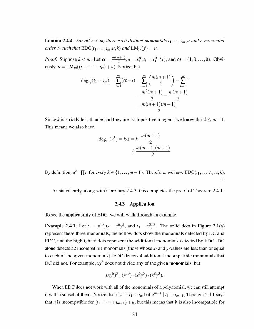
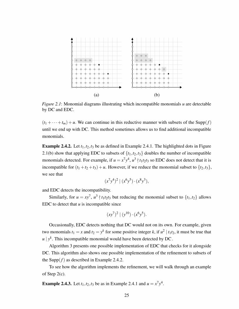
Example 2.4.1. Let t1 = y10, t2 = x6y5, and t3 = x8y3. The solid dots in Figure 2.1(a)represent these three monomials, the hollow dots show the monomials detected by DC andEDC, and the highlighted dots represent the additional monomials detected by EDC . DCalone detects 52 incompatible monomials (those whose x- and y-values are less than or equalto each of the given monomials). EDC detects 4 additional incompatible monomials thatDC did not. For example, xy6 does not divide any of the given monomials, but
(xy6)3 | (y10) · (x6y5) · (x8y3).
When EDC does not work with all of the monomials of a polynomial, we can still attemptit with a subset of them. Notice that if um - t1 · · · tm but um−1 | t1 · · · tm−1, Theorem 2.4.1 saysthat u is incompatible for (t1 + · · ·+ tm−1)+u, but this means that it is also incompatible for
24
(a) (b)
Figure 2.1: Monomial diagrams illustrating which incompatible monomials u are detectableby DC and EDC.
(t1 + · · ·+ tm)+u. We can continue in this reductive manner with subsets of the Supp( f )
until we end up with DC. This method sometimes allows us to find additional incompatiblemonomials.
Example 2.4.2. Let t1, t2, t3 be as defined in Example 2.4.1. The highlighted dots in Figure2.1(b) show that applying EDC to subsets of {t1, t2, t3} doubles the number of incompatiblemonomials detected. For example, if u = x7y4, u3 - t1t2t3 so EDC does not detect that it isincompatible for (t1 + t2 + t3)+u. However, if we reduce the monomial subset to {t2, t3},we see that
(x7y4)2 | (x6y5) · (x8y3),
and EDC detects the incompatibility.Similarly, for u = xy7, u3 - t1t2t3 but reducing the monomial subset to {t1, t2} allows
EDC to detect that u is incompatible since
(xy7)2 | (y10) · (x6y5).
Occasionally, EDC detects nothing that DC would not on its own. For example, giventwo monomials t1 = x and t2 = yk for some positive integer k, if u2 | t1t2, it must be true thatu | yk. This incompatible monomial would have been detected by DC .
Algorithm 3 presents one possible implementation of EDC that checks for it alongsideDC. This algorithm also shows one possible implementation of the refinement to subsets ofthe Supp( f ) as described in Example 2.4.2.
To see how the algorithm implements the refinement, we will walk through an exampleof Step 2(c).
Example 2.4.3. Let t1, t2, t3 be as in Example 2.4.1 and u = x7y4.
25
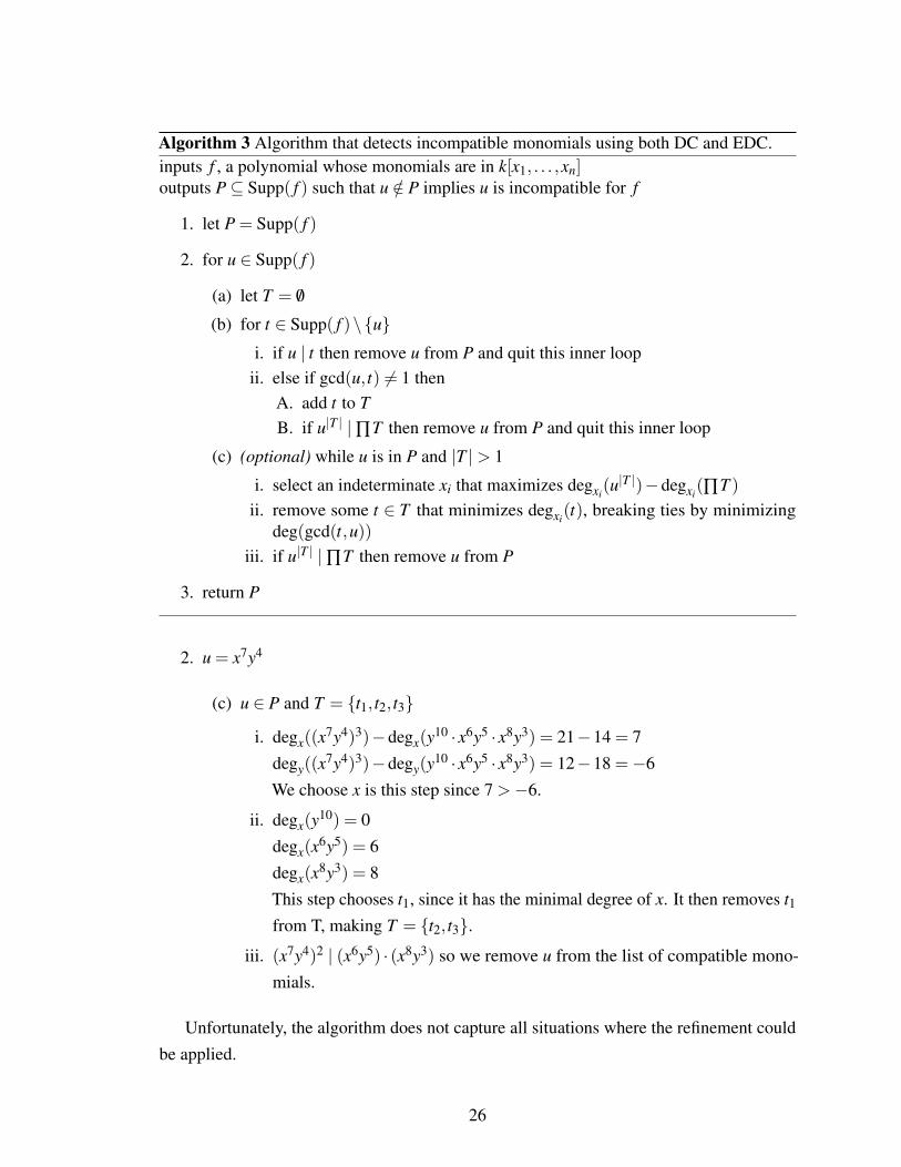
Algorithm 3 Algorithm that detects incompatible monomials using both DC and EDC.inputs f , a polynomial whose monomials are in k[x1, . . . ,xn]outputs P⊆ Supp( f ) such that u /∈ P implies u is incompatible for f
1. let P = Supp( f )
2. for u ∈ Supp( f )
(a) let T = /0
(b) for t ∈ Supp( f )\{u}i. if u | t then remove u from P and quit this inner loop
ii. else if gcd(u, t) 6= 1 thenA. add t to TB. if u|T | |∏T then remove u from P and quit this inner loop
(c) (optional) while u is in P and |T |> 1
i. select an indeterminate xi that maximizes degxi(u|T |)−degxi
(∏T )ii. remove some t ∈ T that minimizes degxi
(t), breaking ties by minimizingdeg(gcd(t,u))
iii. if u|T | |∏T then remove u from P
3. return P
2. u = x7y4
(c) u ∈ P and T = {t1, t2, t3}
i. degx((x7y4)3)−degx(y
10 · x6y5 · x8y3) = 21−14 = 7degy((x
7y4)3)−degy(y10 · x6y5 · x8y3) = 12−18 =−6
We choose x is this step since 7 >−6.
ii. degx(y10) = 0
degx(x6y5) = 6
degx(x8y3) = 8
This step chooses t1, since it has the minimal degree of x. It then removes t1from T, making T = {t2, t3}.
iii. (x7y4)2 | (x6y5) · (x8y3) so we remove u from the list of compatible mono-mials.
Unfortunately, the algorithm does not capture all situations where the refinement couldbe applied.
26
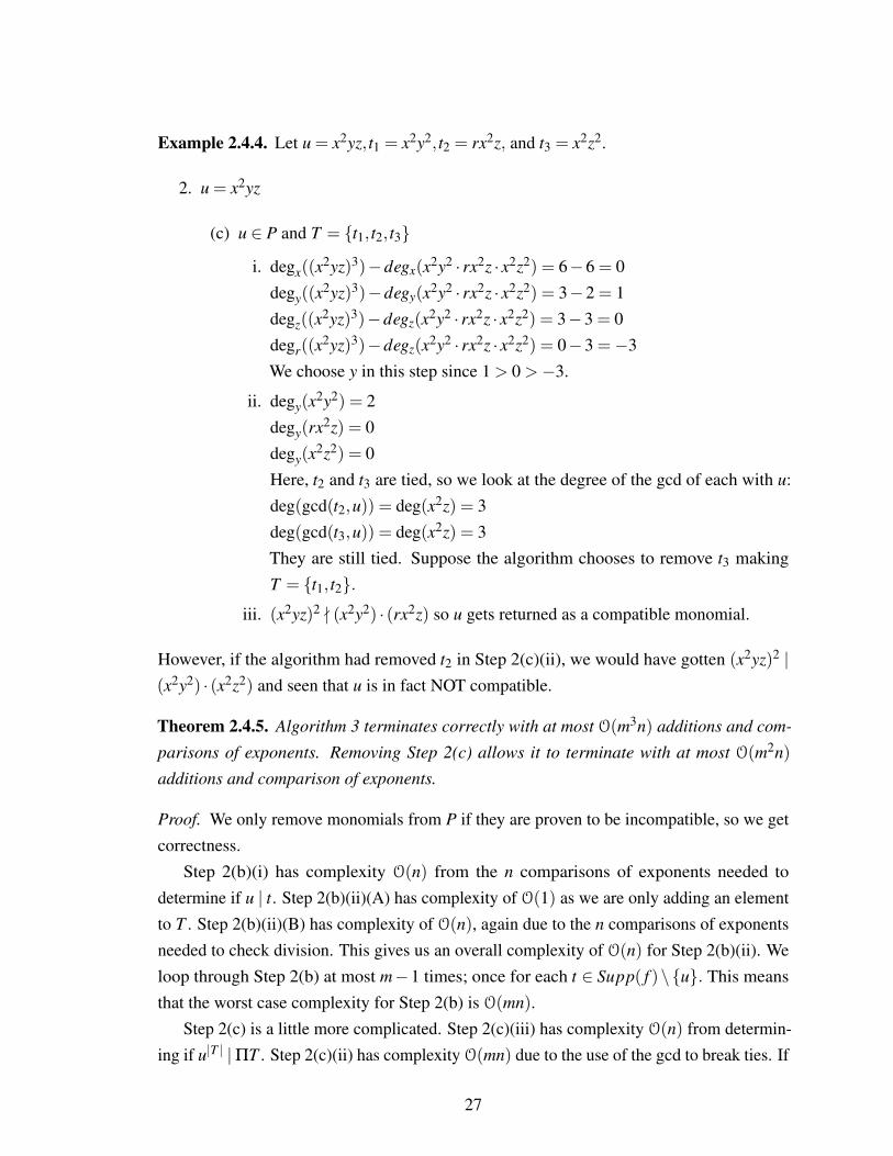
Example 2.4.4. Let u = x2yz, t1 = x2y2, t2 = rx2z, and t3 = x2z2.
2. u = x2yz
(c) u ∈ P and T = {t1, t2, t3}
i. degx((x2yz)3)−degx(x2y2 · rx2z · x2z2) = 6−6 = 0
degy((x2yz)3)−degy(x2y2 · rx2z · x2z2) = 3−2 = 1
degz((x2yz)3)−degz(x2y2 · rx2z · x2z2) = 3−3 = 0
degr((x2yz)3)−degz(x2y2 · rx2z · x2z2) = 0−3 =−3
We choose y in this step since 1 > 0 >−3.
ii. degy(x2y2) = 2
degy(rx2z) = 0degy(x
2z2) = 0Here, t2 and t3 are tied, so we look at the degree of the gcd of each with u:deg(gcd(t2,u)) = deg(x2z) = 3deg(gcd(t3,u)) = deg(x2z) = 3They are still tied. Suppose the algorithm chooses to remove t3 makingT = {t1, t2}.
iii. (x2yz)2 - (x2y2) · (rx2z) so u gets returned as a compatible monomial.
However, if the algorithm had removed t2 in Step 2(c)(ii), we would have gotten (x2yz)2 |(x2y2) · (x2z2) and seen that u is in fact NOT compatible.
Theorem 2.4.5. Algorithm 3 terminates correctly with at most O(m3n) additions and com-
parisons of exponents. Removing Step 2(c) allows it to terminate with at most O(m2n)
additions and comparison of exponents.
Proof. We only remove monomials from P if they are proven to be incompatible, so we getcorrectness.
Step 2(b)(i) has complexity O(n) from the n comparisons of exponents needed todetermine if u | t. Step 2(b)(ii)(A) has complexity of O(1) as we are only adding an elementto T . Step 2(b)(ii)(B) has complexity of O(n), again due to the n comparisons of exponentsneeded to check division. This gives us an overall complexity of O(n) for Step 2(b)(ii). Weloop through Step 2(b) at most m−1 times; once for each t ∈ Supp( f )\{u}. This meansthat the worst case complexity for Step 2(b) is O(mn).
Step 2(c) is a little more complicated. Step 2(c)(iii) has complexity O(n) from determin-ing if u|T | |ΠT . Step 2(c)(ii) has complexity O(mn) due to the use of the gcd to break ties. If
27
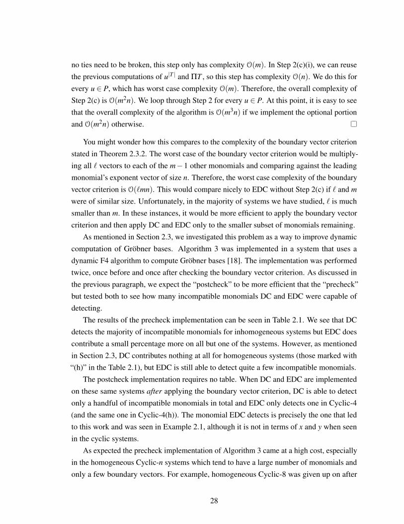
no ties need to be broken, this step only has complexity O(m). In Step 2(c)(i), we can reusethe previous computations of u|T | and ΠT , so this step has complexity O(n). We do this forevery u ∈ P, which has worst case complexity O(m). Therefore, the overall complexity ofStep 2(c) is O(m2n). We loop through Step 2 for every u ∈ P. At this point, it is easy to seethat the overall complexity of the algorithm is O(m3n) if we implement the optional portionand O(m2n) otherwise.
You might wonder how this compares to the complexity of the boundary vector criterionstated in Theorem 2.3.2. The worst case of the boundary vector criterion would be multiply-ing all ` vectors to each of the m−1 other monomials and comparing against the leadingmonomial’s exponent vector of size n. Therefore, the worst case complexity of the boundaryvector criterion is O(`mn). This would compare nicely to EDC without Step 2(c) if ` and m
were of similar size. Unfortunately, in the majority of systems we have studied, ` is muchsmaller than m. In these instances, it would be more efficient to apply the boundary vectorcriterion and then apply DC and EDC only to the smaller subset of monomials remaining.
As mentioned in Section 2.3, we investigated this problem as a way to improve dynamiccomputation of Gröbner bases. Algorithm 3 was implemented in a system that uses adynamic F4 algorithm to compute Gröbner bases [18]. The implementation was performedtwice, once before and once after checking the boundary vector criterion. As discussed inthe previous paragraph, we expect the “postcheck” to be more efficient that the “precheck”but tested both to see how many incompatible monomials DC and EDC were capable ofdetecting.
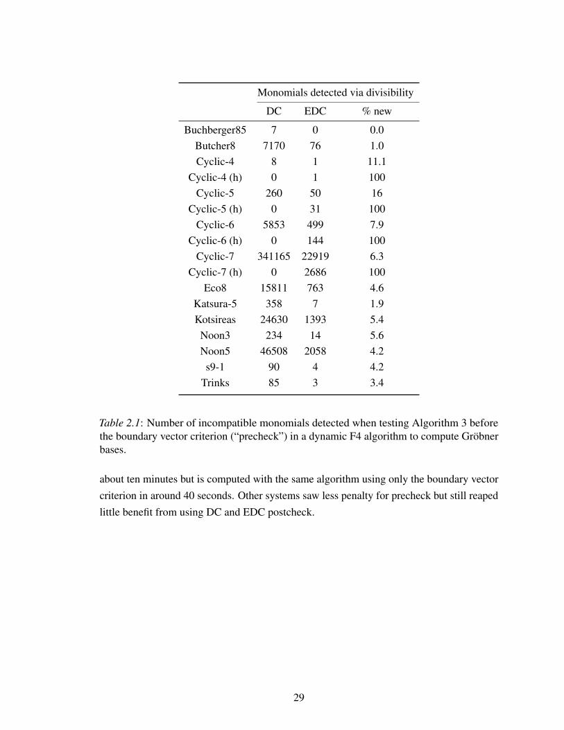
The results of the precheck implementation can be seen in Table 2.1. We see that DCdetects the majority of incompatible monomials for inhomogeneous systems but EDC doescontribute a small percentage more on all but one of the systems. However, as mentionedin Section 2.3, DC contributes nothing at all for homogeneous systems (those marked with“(h)” in the Table 2.1), but EDC is still able to detect quite a few incompatible monomials.
The postcheck implementation requires no table. When DC and EDC are implementedon these same systems after applying the boundary vector criterion, DC is able to detectonly a handful of incompatible monomials in total and EDC only detects one in Cyclic-4(and the same one in Cyclic-4(h)). The monomial EDC detects is precisely the one that ledto this work and was seen in Example 2.1, although it is not in terms of x and y when seenin the cyclic systems.
As expected the precheck implementation of Algorithm 3 came at a high cost, especiallyin the homogeneous Cyclic-n systems which tend to have a large number of monomials andonly a few boundary vectors. For example, homogeneous Cyclic-8 was given up on after
28
Monomials detected via divisibility
DC EDC % new
Buchberger85 7 0 0.0Butcher8 7170 76 1.0Cyclic-4 8 1 11.1
Cyclic-4 (h) 0 1 100Cyclic-5 260 50 16
Cyclic-5 (h) 0 31 100Cyclic-6 5853 499 7.9
Cyclic-6 (h) 0 144 100Cyclic-7 341165 22919 6.3
Cyclic-7 (h) 0 2686 100Eco8 15811 763 4.6
Katsura-5 358 7 1.9Kotsireas 24630 1393 5.4
Noon3 234 14 5.6Noon5 46508 2058 4.2s9-1 90 4 4.2
Trinks 85 3 3.4
Table 2.1: Number of incompatible monomials detected when testing Algorithm 3 beforethe boundary vector criterion (“precheck”) in a dynamic F4 algorithm to compute Gröbnerbases.
about ten minutes but is computed with the same algorithm using only the boundary vectorcriterion in around 40 seconds. Other systems saw less penalty for precheck but still reapedlittle benefit from using DC and EDC postcheck.
29
Chapter 3
Dynamic Gröbner Basis Computation
3.1 Introduction
As demonstrated in Chapter 2, the outcome of traditional Gröbner basis algorithms isdependent on the choice of monomial order, and some monomial orders lead to smallerbases than others. However, using a traditional algorithm, it is difficult to know which willbe better without running the algorithm in its entirety on many different orderings. Thereare an infinite number of choices for monomial orders, so a brute force search can neverguarantee that it has found the smallest Gröbner basis.
Researchers wondered if there was a method that could identify a “better” order. Theauthors of [17] investigated the Gröbner fan of an ideal. This fan looks at the polyhedralcones associated with sets of monomial orders, Σ, where for each σ ∈ Σ, the reducedGröbner bases of the ideal with respect to σ are the same. They also proved that there areonly finitely many such cones; however, the number of cones may be very large. Theypropose an algorithm that computes the basis for each of these fans independently. Of these,the computation that terminates first is said to yield the smallest Gröbner basis for the givenideal. They admit to having no way to determine which computation will terminate firstbefore completion.
Say that the orders σ and τ are related if I has the same reduced Gröbner basis withrespect to both σ and τ . It is easy to see that this is an equivalence relation and the previousparagraph’s polyhedral cones are the equivalence classes. The reader likely noticed that,for a fixed ideal, there are finitely many equivalence classes of monomials orders. Thisalso means that there are finitely many Gröbner bases. Instead of a brute force search on“all” the monomial orders, we could compute the Gröbner fan, then compute the Gröbnerbasis for one monomial order in each equivalence class. However, this is also infeasible, ascomputing a Gröbner fan consumes significant amounts of time and memory.
In 1993, [3] and [12] independently proposed a dynamic Buchberger algorithm thatallows the monomial order to vary at the start of each S-polynomial loop if doing so wouldlead to a smaller Gröbner basis. They minimize the Hilbert function in an attempt to identifythis “preferable” order.
30
Definition 3.1.1 (Definition 2 of §9.3 in [5]). Let I ∈ k[x1, . . . ,xn] be an ideal. Let Rs =
k[x1, . . . ,xn]s represent the set of polynomials with degree s in k[x1, . . . ,xn] and Is representthe set of polynomials in I with degree s. The Hilbert function is the function
HFR/I(s) = dimRs/Is = dimRs−dim Is.
By Definition 3.1.1 and Proposition 3 in §9.3 of [5], we know that given an ideal ofmonomials in k[x1, . . . ,xn], the Hilbert function identifies the number of monomials at eachdegree that are not in the ideal. By Definition 1.3.1, we know that we have a Gröbner basisfor an ideal I when the ideal of leading terms in the basis equals the ideal of leading termsin I.
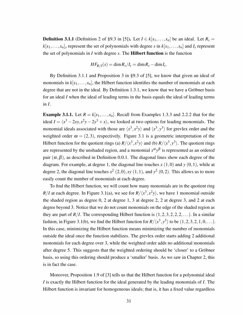
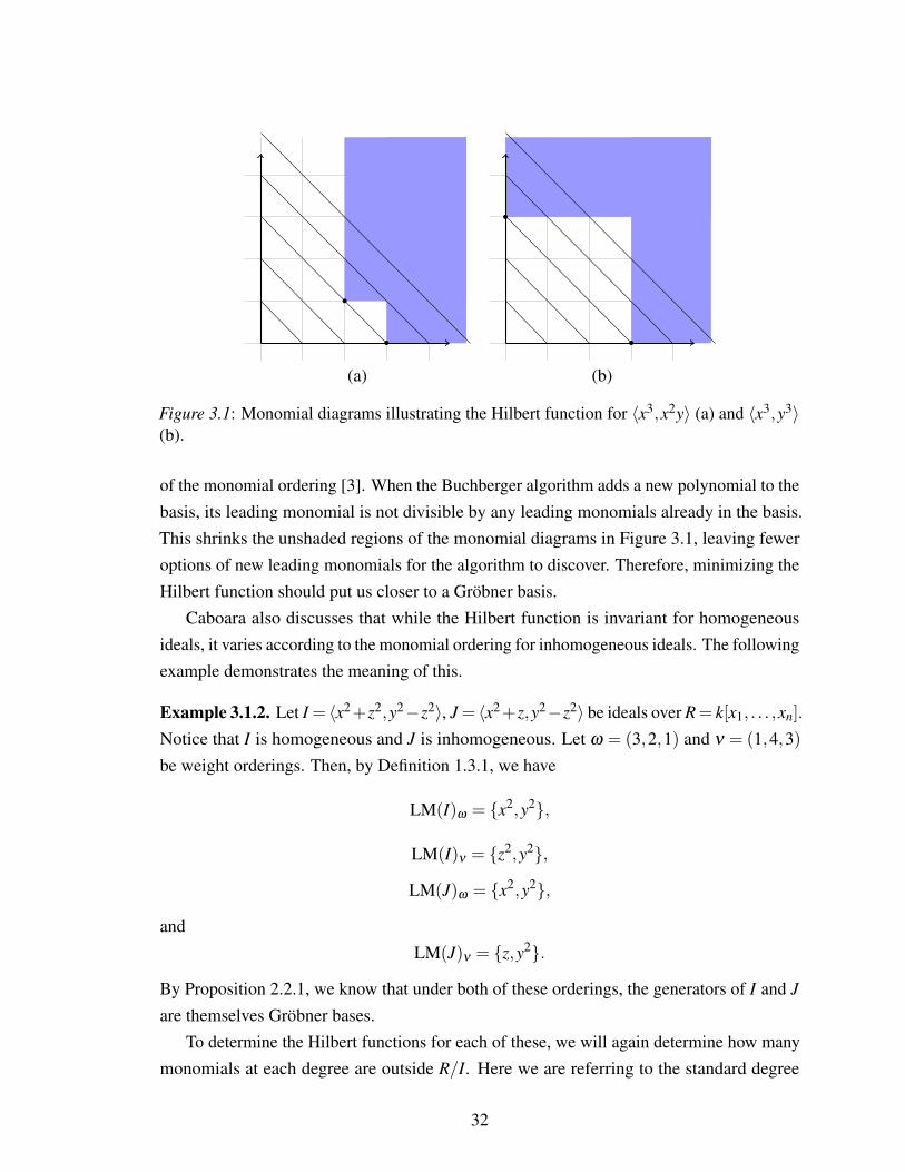
Example 3.1.1. Let R = k[x1, . . . ,xn]. Recall from Examples 1.3.3 and 2.2.2 that for theideal I = 〈x3−2xy,x2y−2y3 + x〉, we looked at two options for leading monomials. Themonomial ideals associated with those are 〈x3,x2y〉 and 〈x3,y3〉 for grevlex order and theweighted order ω = (2,3), respectively. Figure 3.1 is a geometric interpretation of theHilbert function for the quotient rings (a) R/〈x3,x2y〉 and (b) R/〈x3,y3〉. The quotient ringsare represented by the unshaded region, and a monomial xαyβ is represented as an orderedpair (α,β ), as described in Definition 0.0.1. The diagonal lines show each degree of thediagram. For example, at degree 1, the diagonal line touches x (1,0) and y (0,1), while atdegree 2, the diagonal line touches x2 (2,0),xy (1,1), and y2 (0,2). This allows us to moreeasily count the number of monomials at each degree.
To find the Hilbert function, we will count how many monomials are in the quotient ringR/I at each degree. In Figure 3.1(a), we see for R/〈x3,x2y〉, we have 1 monomial outsidethe shaded region as degree 0, 2 at degree 1, 3 at degree 2, 2 at degree 3, and 2 at eachdegree beyond 3. Notice that we do not count monomials on the edge of the shaded region asthey are part of R/I. The corresponding Hilbert function is (1,2,3,2,2,2, . . .). In a similarfashion, in Figure 3.1(b), we find the Hilbert function for R/〈x3,y3〉 to be (1,2,3,2,1,0, . . .).In this case, minimizing the Hilbert function means minimizing the number of monomialsoutside the ideal once the function stabilizes. The grevlex order starts adding 2 additionalmonomials for each degree over 3, while the weighted order adds no additional monomialsafter degree 5. This suggests that the weighted ordering should be ‘closer’ to a Gröbnerbasis, so using this ordering should produce a ‘smaller’ basis. As we saw in Chapter 2, thisis in fact the case.
Moreover, Proposition 1.9 of [3] tells us that the Hilbert function for a polynomial idealI is exactly the Hilbert function for the ideal generated by the leading monomials of I. TheHilbert function is invariant for homogeneous ideals; that is, it has a fixed value regardless
31
(a) (b)
Figure 3.1: Monomial diagrams illustrating the Hilbert function for 〈x3,x2y〉 (a) and 〈x3,y3〉(b).
of the monomial ordering [3]. When the Buchberger algorithm adds a new polynomial to thebasis, its leading monomial is not divisible by any leading monomials already in the basis.This shrinks the unshaded regions of the monomial diagrams in Figure 3.1, leaving feweroptions of new leading monomials for the algorithm to discover. Therefore, minimizing theHilbert function should put us closer to a Gröbner basis.
Caboara also discusses that while the Hilbert function is invariant for homogeneousideals, it varies according to the monomial ordering for inhomogeneous ideals. The followingexample demonstrates the meaning of this.
Example 3.1.2. Let I = 〈x2+z2,y2−z2〉, J = 〈x2+z,y2−z2〉 be ideals over R= k[x1, . . . ,xn].Notice that I is homogeneous and J is inhomogeneous. Let ω = (3,2,1) and ν = (1,4,3)be weight orderings. Then, by Definition 1.3.1, we have
LM(I)ω = {x2,y2},
LM(I)ν = {z2,y2},
LM(J)ω = {x2,y2},
andLM(J)ν = {z,y2}.
By Proposition 2.2.1, we know that under both of these orderings, the generators of I and J
are themselves Gröbner bases.To determine the Hilbert functions for each of these, we will again determine how many
monomials at each degree are outside R/I. Here we are referring to the standard degree
32
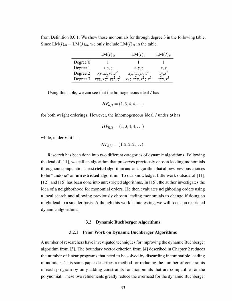
from Definition 0.0.1. We show those monomials for through degree 3 in the following table.Since LM(I)ω = LM(J)ω , we only include LM(I)ω in the table.
LM(I)ω LM(I)ν LM(J)ν
Degree 0 1 1 1Degree 1 x,y,z x,y,z x,yDegree 2 xy,xz,yz,z2 xy,xz,yz,x2 xy,x2
Degree 3 xyz,xz2,yz2,z3 xyz,x2y,x2z,x3 x2y,x3
Using this table, we can see that the homogeneous ideal I has
HFR/I = (1,3,4,4, . . .)
for both weight orderings. However, the inhomogeneous ideal J under ω has
HFR/J = (1,3,4,4, . . .)
while, under ν , it hasHFR/J = (1,2,2,2, . . .).
Research has been done into two different categories of dynamic algorithms. Followingthe lead of [11], we call an algorithm that preserves previously chosen leading monomialsthroughout computation a restricted algorithm and an algorithm that allows previous choicesto be “undone” an unrestricted algorithm. To our knowledge, little work outside of [11],[12], and [15] has been done into unrestricted algorithms. In [15], the author investigates theidea of a neighborhood for monomial orders. He then evaluates neighboring orders usinga local search and allowing previously chosen leading monomials to change if doing somight lead to a smaller basis. Although this work is interesting, we will focus on restricteddynamic algorithms.
3.2 Dynamic Buchberger Algorithms
3.2.1 Prior Work on Dynamic Buchberger Algorithms
A number of researchers have investigated techniques for improving the dynamic Buchbergeralgorithm from [3]. The boundary vector criterion from [4] described in Chapter 2 reducesthe number of linear programs that need to be solved by discarding incompatible leadingmonomials. This same paper describes a method for reducing the number of constraintsin each program by only adding constraints for monomials that are compatible for thepolynomial. These two refinements greatly reduce the overhead for the dynamic Buchberger
33
algorithm. In addition, the original algorithm from [3] had so many linear programs andconstraints that they grew unmanageable, and the algorithm was forced to stop addingadditional constraints and continue as a static algorithm until termination. The boundaryvector criterion allows the algorithm to continue in a dynamic fashion until termination.
Alternative heuristics to the Hilbert heuristic described in 3.1 were explored in [19]. Theauthor investigates four possible heuristics. The first is the Hilbert heuristic, which is basedon the use of the Hilbert function in [12]. This heuristic requires us to define the Hilbertpolynomial, the Hilbert series, and the Hilbert numerator.
Theorem 3.2.1 (Theorem 5.1.21 of [13]). Let R = k[x1, . . . ,xn], I be an ideal, and R/I
be their quotient ring. Then the Hilbert function HFR/I : Z→ Z is an integer function of
polynomial type.
Definition 3.2.1 (Definition 5 of §9.3 in [5]). The Hilbert polynomial of the quotient ringR/I is the polynomial which equals HFR/I(s) for sufficiently large s. It is written HPR/I(s).
We can use well-known tool from discrete mathematics to rewrite any sequence
(a0,a1,a2, . . .)
as a power seriesA = a0 +a1x+a2x2 + . . .
which is called the generating function for (a0,a1,a2, . . .). A thorough discussion on thiscan be found in Chapter 49 of [20], which is available online.
Definition 3.2.2 (Definition 5.2.13 of [13]). The Hilbert series of R/I is the formal powerseries associated with the Hilbert function of R/I. In other words,
HSR/I(z) = ∑i≥0
HFR/I(i)zi.
Definition 3.2.3 (Definition 5.2.21 of [13]). Given a quotient ring R/I and Hilbert series
HSR/I(z) =HNR/I(z)(1− z)n ,
the polynomial HNR/I(z) is called the Hilbert numerator of R/I. (Here, the n in thedenominator refers to the number of variables in R.)
Example 3.2.1. Let R be as in Example 3.1.1. We will also use the same ideals of leadingmonomials, 〈x3,x2y〉 and 〈x3,y3〉.
34
We saw in the previous example that for s≥ 3,
HFR/〈x3,x2y〉(s) = 2,
and for s≥ 5,HFR/〈x3,y3〉(s) = 0.
The corresponding Hilbert polynomials are then
HPR/〈x3,x2y〉 = 2
andHPR/〈x3,y3〉 = 0.
When |z|< 1, the corresponding Hilbert series are
HSR/〈x3,x2y〉 = 1+2z+3z2 +2z3 +∑i≥4
2zi (3.1)
andHSR/〈x3,y3〉 = 1+2z+3z2 +2z3 + z4. (3.2)
Notice in Equation 3.1, we can rewrite ∑i≥4
2zi as
∞
∑i=0
2zi−3
∑i=0
2zi,
where the first term is a geometric series. This allows us to rewrite the Hilbert series as
HSR/〈x3,x2y〉 = 1+2z+3z2 +2z3 +∑i≥4
2zi
= 1+2z+3z2 +2z3 +∞
∑i=0
2zi−3
∑i=0
2zi
= 1+2z+3z2 +2z3 +∞
∑i=0
2zi−2−2z−2z2−2z3
=2
1− z+ z2−1
=2(1− z)+(z2−1)(1− z)2
(1− z)2
=z4−2z3 +1(1− z)2 .
35
Equation 3.2 is easier to rewrite, as we only need to multiply by(1− z)2
(1− z)2 ,
HSR/〈x3,y3〉 = 1+2z+3z2 +2z3 + z4
=(1+2z+3z2 +2z3 + z4)(1− z)2
(1− z)2
=z6−2z3 +1(1− z)2
At this point, it is clear that we have
HNR/〈x3,x2y〉 = z4−2z3 +1
andHNR/〈x3,y3〉 = z6−2z3 +1.
Now, that we understand the meaning of a Hilbert polynomial and a Hilbert numerator,we can define the first heuristic from [19].
Definition 3.2.4. Let G = {g1, . . . ,g`} be the current basis elements, f be the polynomialwe wish to add to the basis, and t1, t2 be possible leading monomials of f . Let hi be theHilbert numerator of 〈LM(G)∪{ti}〉 and pi be the Hilbert polynomial of 〈LM(G)∪{ti}〉.For tuples (h1, p1),(h2, p2), the Hilbert heuristic chooses t1 = LM( f ) if
(i) LC(p1− p2)< 0, or
(ii) p1 = p2 and the “trailing” term of h1−h2 is positive.
In part (ii) of the definition, trailing term means the term of smallest degree. If we use thisheuristic with Example 3.2.1 for t1 = x2y, t2 = y3, we see that
LC(p2− p1) = 0−2 < 0.
Therefore, the Hilbert heuristic would choose y3 to be the leading term.
The next heuristic is the Betti heuristic which attempts to minimize the number ofS-polynomials the algorithm computes by minimizing the number of critical pairs generated.
Definition 3.2.5. Let G, f , t1, t2 be as in Definition 3.2.4. Let Pi be the set of critical pairsqueued to be computed after potentially choosing ti = LM( f ) and adding the new pairsassociated with this choice. The Betti heuristic chooses t1 = LM( f ) if
|P1|< |P2|.
36
The final two heuristics are the “graded” Hilbert and Betti heuristics. These are simplythe previous two heuristics but using the current monomial order instead of the standarddegree. The results of implementing these new heuristics show that the graded heuristicsare generally outperformed by their “ungraded” counterparts. The standard Betti heuristichowever shows promise in some systems and is therefore recognized as a good alternativeto the standard Hilbert heuristic.
Algorithm 4 follows the example of Algorithm 1 in [19] and shows one possible imple-mentation of a dynamic Buchberger algorithm. Section 3.2.2 walks through an examplecomputation using the algorithm. Step 2(a) of the algorithm indicates that we should choosea pair with “minimal sugar.” This strategy for choosing which S-polynomial to computecomes from [10].
Definition 3.2.6 (From Section 2 of [10]). Given a polynomial f , its sugar S f is defined inthe following way:
(i) for the initial fi, S fi = tdeg( f ) (this is the degree from Definition 1.1.1 not the degreewith respect to the monomial order);
(ii) if f is a polynomial and t = xα a monomial, then St f = |α|+S f ;
(iii) if f = g+h, then S f = max(Sg,Sh).
If the sugar strategy fails, we will use the normal selection strategy, meaning choose thepair (p,q) with lowest degree of tp,q.
3.2.2 Dynamic Buchberger Algorithm Example
For our example, we will use one of the famous Cyclic-n systems, specifically Cyclic-4hwhere h indicates that the system is homogenized. Throughout the example, we will makethe polynomials found in Steps 2(b) and 2(c)(iii) monic for ease of computation.
Example 3.2.2. Let
f1 = x1 + x2 + x3 + x4
f2 = x1x2 + x2x3 + x3x4 + x1x4
f3 = x1x2x3 + x2x3x4 + x1x3x4 + x1x2x4
f4 = x1x2x3x4−h4
andI = 〈 f1, f2, f3, f4〉.
37
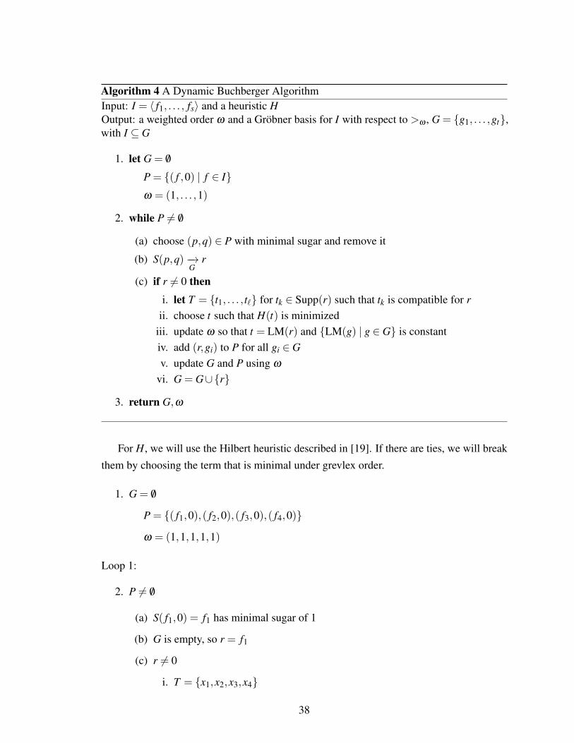
Algorithm 4 A Dynamic Buchberger AlgorithmInput: I = 〈 f1, . . . , fs〉 and a heuristic HOutput: a weighted order ω and a Gröbner basis for I with respect to >ω , G = {g1, . . . ,gt},with I ⊆ G
1. let G = /0
P = {( f ,0) | f ∈ I}ω = (1, . . . ,1)
2. while P 6= /0
(a) choose (p,q) ∈ P with minimal sugar and remove it
(b) S(p,q)−→G
r
(c) if r 6= 0 theni. let T = {t1, . . . , t`} for tk ∈ Supp(r) such that tk is compatible for r
ii. choose t such that H(t) is minimizediii. update ω so that t = LM(r) and {LM(g) | g ∈ G} is constantiv. add (r,gi) to P for all gi ∈ Gv. update G and P using ω
vi. G = G∪{r}
3. return G,ω
For H, we will use the Hilbert heuristic described in [19]. If there are ties, we will breakthem by choosing the term that is minimal under grevlex order.
1. G = /0
P = {( f1,0),( f2,0),( f3,0),( f4,0)}
ω = (1,1,1,1,1)
Loop 1:
2. P 6= /0
(a) S( f1,0) = f1 has minimal sugar of 1
(b) G is empty, so r = f1
(c) r 6= 0
i. T = {x1,x2,x3,x4}
38
ii. Unfortunately, all four Hilbert polynomials and all four Hilbert numeratorsare equal. We choose x4 as the smallest monomial with respect to grevlexorder.
iii. ω = (1,1,1,2,1)
iv. G is empty, so we skip this step
v. Throughout this example, we will neglect to show the updated elements of P
and previous elements of G, but you will encounter the updated polynomialsin other loops or when the basis is returned.
vi. G = {x4 + x1 + x2 + x3}
Loop 2:
2. (a) S( f2,0) = x1x4 + x3x4 + x1x2 + x2x3 has minimal sugar of 2
(b) r = x21 +2x1x3 + x2
3
(c) i. T = {x21,x
23}
(We are able to remove x1x3 by Theorem 2.4.1)
ii. Again, both Hilbert polynomials and both Hilbert numerators are equal.The smallest monomial under grevlex order is x2
3.
iii. ω = (1,1,2,3,1)
iv. By Proposition 2.2.1, we do not need to compute S(r,g1). We have P =
{( f3,0),( f4,0)}
vi. G = G∪{x23 +2x1x3 + x2
1}
Loop 3:
2. (a) S( f3,0) = x1x3x4 + x2x3x4 + x1x2x4 + x1x2x3 has minimal sugar of 3
(b) r = x21x3− x2
2x3 + x31− x1x2
2
(c) i. T = {x21x3,x2
2x3}
ii. Again, both Hilbert polynomials and both Hilbert numerators are equal.The smallest monomial under grevlex order is x2
2x3.
iii. update ω = (1,2,2,3,1)
iv. P = {( f4,0),(r,g2)}
vi. G = G∪{x22x3 + x1x2
2− x21x3− x3
1}
Loop 4:
39

2. (a) SS(g3,g2) = 4 and S f4 = 4. The sugar strategy has failed us, so we choose (g3,g2),the pair with lowest degree.
(b) r = 0
Loop 5:
2. (a) ( f4,0) is the only element in P
(b) r = x21x2
2 + x21x2x3 + x3
1x2− x31x3− x4
1−h4
(c) i. T = {x21x2
2,x21x2x3,h4}. We will call these t1, t2, t3.
ii. h1 =−t6 + t5 + t4− t2− t +1h2 = t7−3t6 +2t5 + t4− t2− t +1h3 = t9−2t8 + t6 + t4− t2− t +1
p1 = 6t−3p2 =
12t2 + 5
2t +3p3 =−4t−6
LT(p3− p1) = −10t and all others are positive, so we choose h4 as theLM(r).
iii. update ω = (1,2,2,3,7)
iv. We add no new pairs by Proposition 2.2.1, so P = /0
vi. G = G∪{h4− x21x2
2− x21x2x3− x3
1x2 + x31x3 + x4
1}
3. return G,ω
So, we have found a Gröbner basis,
G = {x4 + x2 + x3 + x1,x23 +2x1x3 + x2
1,
x22x3 + x1x2
2− x21x3− x3
1,h4− x2
1x22− x2
1x2x3− x31x2 + x3
1x3 + x41},
for ω = (1,2,2,3,7) by computing only 5 S-polynomials, and the basis contains just 4elements. To put this in perspective, the static Buchberger algorithm using grevlex ordercomputes 12 S-polynomials and returns a Gröbner basis with 7 elements.
3.3 A Dynamic F4 Algorithm
3.3.1 Background
The F4 algorithm was first presented by Faugére in [9]. He used notions from linear algebrato relate the polynomial ring, k[x1, . . . ,xn], to a vector space and the Buchberger algorithm toGaussian elimination using the Macaulay matrix described by [16], which is a generalizationof the Sylvester matrix. In the F4 algorithm, the columns of a matrix M correspond to
40
the monomials in M in descending order, according to some monomial order. Faugérerecommends using grevlex order as it is well known to terminate with a Gröbner basis at alower degree than other orders. Given an ideal I = 〈 f1, . . . , fm〉, the rows of M correspond tothe coefficients of the polynomials fi in B⊆ I, where deg( fi) = deg( f j) for all fi, f j ∈ B as
well as the coefficients of the multiples m fi with m ∈M, fi ∈ B. Clearly, this is an infinitematrix. However, if we are restricted to finite submatrices, it becomes more manageable. In[9], Faugére showed that this method was able to compute Gröbner bases for polynomialideals that were previously intractable.
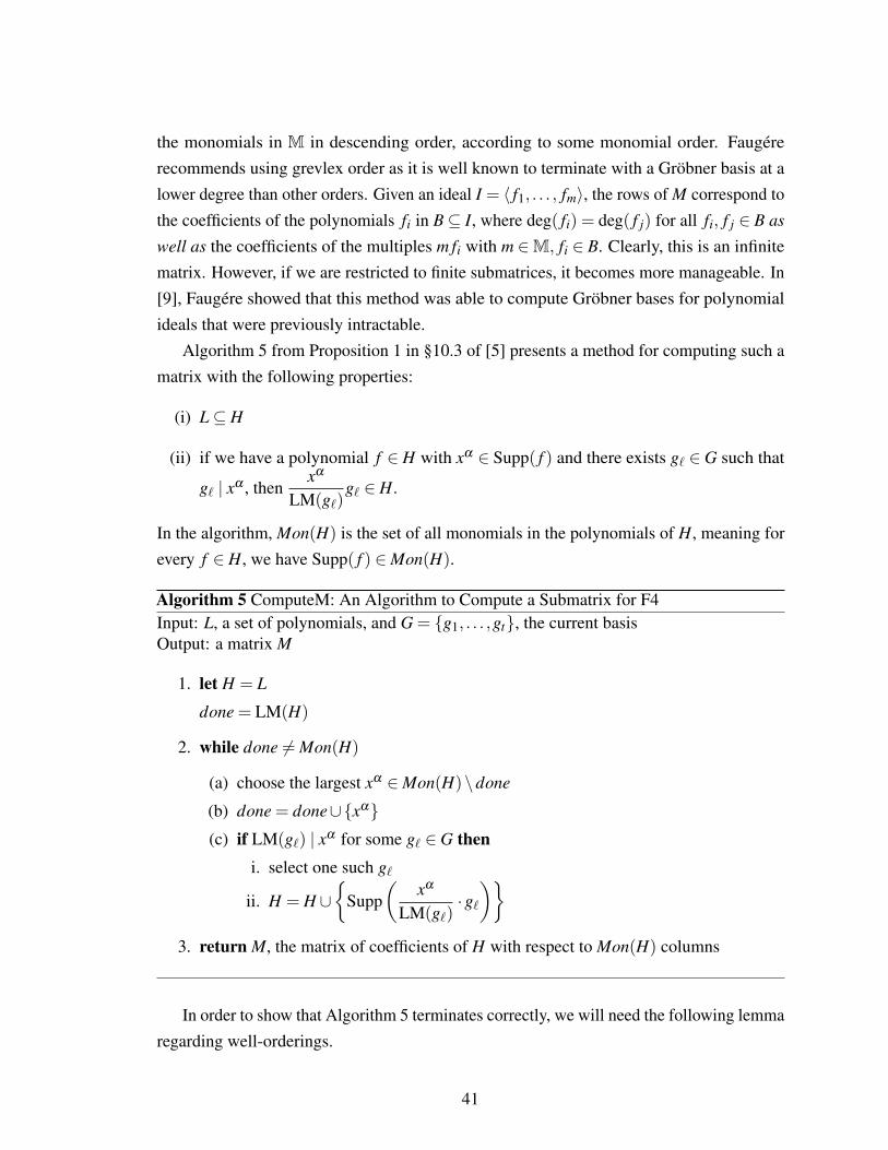
Algorithm 5 from Proposition 1 in §10.3 of [5] presents a method for computing such amatrix with the following properties:
(i) L⊆ H
(ii) if we have a polynomial f ∈ H with xα ∈ Supp( f ) and there exists g` ∈ G such that
g` | xα , thenxα
LM(g`)g` ∈ H.
In the algorithm, Mon(H) is the set of all monomials in the polynomials of H, meaning forevery f ∈ H, we have Supp( f ) ∈Mon(H).
Algorithm 5 ComputeM: An Algorithm to Compute a Submatrix for F4Input: L, a set of polynomials, and G = {g1, . . . ,gt}, the current basisOutput: a matrix M
1. let H = L
done = LM(H)
2. while done 6= Mon(H)
(a) choose the largest xα ∈Mon(H)\done
(b) done = done∪{xα}(c) if LM(g`) | xα for some g` ∈ G then
i. select one such g`
ii. H = H ∪{
Supp(
xα
LM(g`)·g`)}
3. return M, the matrix of coefficients of H with respect to Mon(H) columns
In order to show that Algorithm 5 terminates correctly, we will need the following lemmaregarding well-orderings.
41
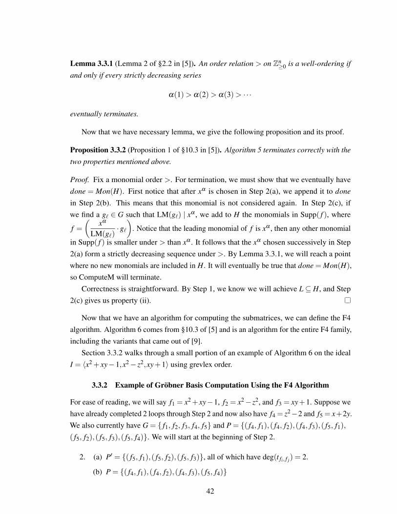
Lemma 3.3.1 (Lemma 2 of §2.2 in [5]). An order relation > on Zn≥0 is a well-ordering if
and only if every strictly decreasing series
α(1)> α(2)> α(3)> · · ·
eventually terminates.
Now that we have necessary lemma, we give the following proposition and its proof.
Proposition 3.3.2 (Proposition 1 of §10.3 in [5]). Algorithm 5 terminates correctly with the
two properties mentioned above.
Proof. Fix a monomial order >. For termination, we must show that we eventually havedone = Mon(H). First notice that after xα is chosen in Step 2(a), we append it to done
in Step 2(b). This means that this monomial is not considered again. In Step 2(c), ifwe find a g` ∈ G such that LM(g`) | xα , we add to H the monomials in Supp( f ), where
f =(
xα
LM(g`)·g`)
. Notice that the leading monomial of f is xα , then any other monomial
in Supp( f ) is smaller under > than xα . It follows that the xα chosen successively in Step2(a) form a strictly decreasing sequence under >. By Lemma 3.3.1, we will reach a pointwhere no new monomials are included in H. It will eventually be true that done = Mon(H),so ComputeM will terminate.
Correctness is straightforward. By Step 1, we know we will achieve L⊆ H, and Step2(c) gives us property (ii).
Now that we have an algorithm for computing the submatrices, we can define the F4algorithm. Algorithm 6 comes from §10.3 of [5] and is an algorithm for the entire F4 family,including the variants that came out of [9].
Section 3.3.2 walks through a small portion of an example of Algorithm 6 on the idealI = 〈x2 + xy−1,x2− z2,xy+1〉 using grevlex order.
3.3.2 Example of Gröbner Basis Computation Using the F4 Algorithm
For ease of reading, we will say f1 = x2+xy−1, f2 = x2− z2, and f3 = xy+1. Suppose wehave already completed 2 loops through Step 2 and now also have f4 = z2−2 and f5 = x+2y.We also currently have G = { f1, f2, f3, f4, f5} and P = {( f4, f1),( f4, f2),( f4, f3),( f5, f1),
( f5, f2),( f5, f3),( f5, f4)}. We will start at the beginning of Step 2.
2. (a) P′ = {( f5, f1),( f5, f2),( f5, f3)}, all of which have deg(t fi, f j) = 2.
(b) P = {( f4, f1),( f4, f2),( f4, f3),( f5, f4)}
42
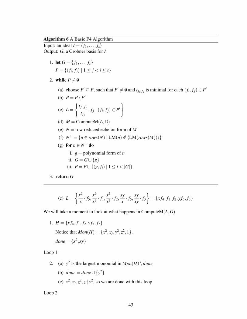
Algorithm 6 A Basic F4 AlgorithmInput: an ideal I = 〈 f1, . . . , fs〉Output: G, a Gröbner basis for I
1. let G = { f1, . . . , fs}P = {( fi, f j) | 1≤ j < i≤ s}
2. while P 6= /0
(a) choose P′ ⊆ P, such that P′ 6= /0 and t fi, f j is minimal for each ( fi, f j) ∈ P′
(b) P = P\P′
(c) L =
{t fi, f j
t f j
· f j | ( fi, f j) ∈ P′}
(d) M = ComputeM(L,G)
(e) N = row reduced echelon form of M
(f) N+ = {n ∈ rows(N) | LM(n) /∈ 〈LM(rows(M))〉}(g) for n ∈ N+ do
i. g = polynomial form of nii. G = G∪{g}
iii. P = P∪{(g, fi) | 1≤ i < |G|}
3. return G
(c) L =
{x2
x· f5,
x2
x2 · f1,x2
x2 · f2,xyx· f5,
xyxy· f3
}= {x f4, f1, f2,y f5, f3}
We will take a moment to look at what happens in ComputeM(L,G).
1. H = {x f4, f1, f2,y f5, f3}
Notice that Mon(H) = {x2,xy,y2,z2,1}.
done = {x2,xy}
Loop 1:
2. (a) y2 is the largest monomial in Mon(H)\done
(b) done = done∪{y2}
(c) x2,xy,z2,z - y2, so we are done with this loop
Loop 2:
43
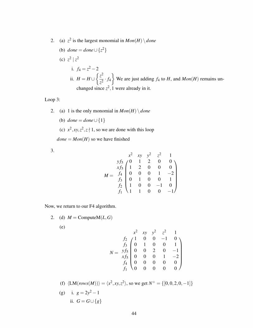
2. (a) z2 is the largest monomial in Mon(H)\done
(b) done = done∪{z2}
(c) z2 | z2
i. f4 = z2−2
ii. H = H ∪{
z2
z2 · f4
}We are just adding f4 to H, and Mon(H) remains un-
changed since z2,1 were already in it.
Loop 3:
2. (a) 1 is the only monomial in Mon(H)\done
(b) done = done∪{1}
(c) x2,xy,z2,z - 1, so we are done with this loop
done = Mon(H) so we have finished
3.
M =
x2 xy y2 z2 1
y f5 0 1 2 0 0x f5 1 2 0 0 0f4 0 0 0 1 −2f3 0 1 0 0 1f2 1 0 0 −1 0f1 1 1 0 0 −1
Now, we return to our F4 algorithm.
2. (d) M = ComputeM(L,G)
(e)
N =
x2 xy y2 z2 1
f2 1 0 0 −1 0f3 0 1 0 0 1
y f5 0 0 2 0 −1x f5 0 0 0 1 −2f4 0 0 0 0 0f1 0 0 0 0 0
(f) 〈LM(rows(M))〉= 〈x2,xy,z2〉, so we get N+ = {[0,0,2,0,−1]}
(g) i. g = 2y2−1
ii. G = G∪{g}
44
iii. P = P∪{(g, f5),(g, f4),(g, f3),(g, f2),(g, f1)}
We will end the example at this point. There are two more loops needed to complete thealgorithm; however, neither of them add any new elements to G. This means that the G atthe end of our example is the Gröbner basis for I under grevlex order.
3.3.3 A Dynamic F4 Algorithm
Unlike dynamic Buchberger algorithms, it seems that little work has been done into a dy-namic F4 algorithm. However, in [18], Perry discusses the advantages of such an algorithm.From the linear algebra perspective, consider the matrix
1 1 1 11 1 1 01 1 0 01 0 0 0
.
Gaussian reduction would take n−1 row reductions. Notice that if we use column swapping,we can obtain a matrix in row-echelon form with
⌊n2
⌋column swaps. In this example matrix
3 versus 2 is not much different in terms of work. However, as the number of rows grows, itwould be a substantial change.
In terms of an F4 algorithm, column swapping amounts to reordering the monomials,especially the leading monomials that we are always concerned with. This means that ifwe allow for some column swapping, there is potential for a dynamic F4 algorithm. Inthe dynamic F4 algorithm described in [18], many of the characteristics used to create adynamic Buchberger algorithm are still in use. For example, the algorithm passes a heuristicfor determining a preferable leading monomial. It is also a restricted algorithm, so it onlymakes changes to the monomial order if doing so does not change previously chosen leadingmonomials.
One of the major changes noted by the author is that interreduction between rows is notallowed. This means that once the newest subset of pairs have been added to a matrix, theycannot be used to reduce each other; however, elements that were previously added to thebasis can be used. This is an effort to preserve previously chosen leading monomials and,typically, means that the output is not in row-echelon form. However, the matrix would stillbe able to remove rows that consist only of zeros. The algorithm then chooses one of thesenonzero rows and picks a leading monomial for it. After this choice is made, the matrix canbe interreduced by the row whose leading monomial is now “set.” There is also the optionto analyze all of the rows simultaneously to choose an overall preferable leading monomial.
This dynamic F4 algorithm shows promising results. Like dynamic Buchberger algo-rithms, it generally returns a Gröbner basis of smaller size than its static counterpart. In
45

many cases, it also computes a smaller basis than the dynamic Buchberger algorithm thoughnot on the same scale as the reduction in size from a static F4 algorithm. For instance, withthe Cyclic-8h polynomials, the static Buchberger and F4 algorithms compute Gröbner basesfor grevlex order of the same size, 1182; while the dynamic Buchberger algorithm findsa basis almost one-third that size with 415 elements. For this same system, the dynamicF4 algorithm that proceeds with one row at a time returns a basis with 402 elements, andthe one that processes all rows simultaneously returns a basis with 403 elements. Theseare much smaller that the static F4 algorithm and smaller but not significantly so than thedynamic Buchberger algorithm.
46
Chapter 4
F5 Algorithm
4.1 Background
Recall in Chapters 1 and 3 that we computed many S-polynomials that reduced zero. If ouronly goal is to find a Gröbner basis, then these zero polynomials add no new information. Inthat context, it seems like a huge waste of time. In 2002, Jean-Charles Faugére introducedan algorithm called F5 [8]. The algorithm avoids computing S-polynomials for most criticalpairs that reduce to zero, making it incredibly useful. The F5 algorithm computes theGröbner basis incrementally. That is, given a list of polynomials, F = { f1, . . . , fm}, F5computes first the Gröbner basis G1 of 〈 f1〉, then the Gröbner basis G2 of 〈 f1, f2〉. Itcontinues in this fashion, computing each Gröbner basis Gi of the ideal 〈 f1, . . . , fi〉 bybuilding on the previous basis Gi−1 of 〈 f1, . . . , fi−1〉. (It should be noted here that mostresearchers, including Faugére, denote this in the reverse order, where Gi is the basis of〈 fi, . . . , fm〉.)
The main difference in the F5 algorithm and other algorithms to compute Gröbner bases,like Buchberger’s, is the use of signatures. Each polynomial is given a signature based onhow it was computed from the original ideal, I = 〈 f1, . . . , fm〉. These signatures are whatallow the algorithm to detect and avoid many reductions to zero.
Definition 4.1.1. Suppose we have a Gröbner basis G. We use ei to represent the canonicalbasis vector with 1 in the ith position. Let σ ,τ ∈ k[x1, . . . ,xn] be monomials. We define anordering � on σei,τe j in the following way.
If one of the following is true:
(i) i > j or
(ii) i = j and σ > τ under the current monomial order,
thenσei � τe j.
We define a signature in the following way.
47
Definition 4.1.2. Let I = 〈 f1, . . . , fm〉 be an ideal. The signature of a monic polynomialf ∈ I is σei if (σ ,ei) is the smallest pair such that:
(i) f =m
∑j=1
h j f j for some h j ∈ k[x1, . . . ,xn],
(ii) hi+1 = · · ·= hm = 0,
(iii) LM(hi) = σ .
Notice that we can view the result of the S-reduction shown in Chapters 1 and 3 as asimilar vector dot product
f = h ·g =s
∑j=1
h jg j, (4.1)
whereh = (h1, . . . ,hs) ∈ k[x1, . . . ,xn]
s
andg = (g1, . . . ,gs) for g j ∈ G.
Definition 4.1.3 (Definition 1 of [7]). Let f ∈ k[x1, . . . ,xn], we say that f has a G-representationif there exist h1, . . . ,hs ∈ k[x1, . . . ,xn] such
f =s
∑j=1
h jg j
and for each j, either h j = 0 or LM(h j)LM(g j)≤ LM( f ). We can also write f in terms ofthe ideal generators as
f =m
∑j=1
h j f j
which we call the S-representation of f with respect to G. We will omit “with respect to G”when it is clear from context.
This S-representation allows us to add another criterion, which was proven in [16], toTheorem 1.3.2 to get the following theorem.
Theorem 4.1.1 (Theorem 1 of [6]). Let I be a polynomial ideal. Then the following are
equivalent:
• G = {g1, . . . ,gt} is a Gröbner basis of I.
• for all pairs i 6= j,S(gi,g j)−→G
0.
48
• for all pairs i 6= j,S(gi,g j) has an S-representation with respect to G.
Since we are now using signatures, we need to make a slight change to how we reducemodulo G. In line 2(a) of Algorithm 2, we will now say:
if LM(g) | LM( f ) for some g ∈ G AND sig( f )� sig(
t f
tg·g).
This means we can only reduce by an element of G if doing so does not change the signatureof f . We call this a signature safe reduction, and often say it does not cause “signaturecorruption.”
Definition 4.1.4 (Definition 7 of [6] and Defintion 8 of [7]). Let gi,g j ∈G and S = S(gi,g j).
Suppose that σev = sig(S), and|G|
∑λ=1
hλ gλ is a G-representation of S such that for each λ
either hλ = 0 or the signature of the product LM(hλ )gλ satisfies
LM(hλ )sig(gλ )≺ σev
for all λ ∈ {1, . . . , |G|}, except one, say `, where LM(h`)sig(g`) = σev and ` > i, j. We say
S =|G|
∑λ=1
hλ gλ
is a signature preserving S-representation. We may omit signature preserving when it isclear from context.
Remark 4.1.1. Notice that having a signature preserving S-representation implies that thepair gi,g j also has an S-representation as we can write any gλ in terms of the generators of I.
We return to Example 1.3.3 to see how signatures work.
Example 4.1.1. RecallI = 〈x3−2xy,x2y−2y3 + x〉,
f1 = x3−2xy,
f2 = x2y−2y3 + x,
and > is grevlex order. Then f1 = 1 · f1 +0 · f2, so
sig( f1) = e1.
We also have f2 = 0 · f1 +1 · f2, so
sig( f2) = e2.
49
In Equation (1.13), we computed g3 = x · f2− y · f1, so
sig(g3) = xe2.
Finally, in Equation (1.14), we computed
S(g3,g2) = x ·g3− y2 ·g2
g4 =12(x ·g3− y2 ·g2 + y · f2 +
14
f1)
=12
(x · (x · f2− y · f1)− y2 · f2 + y · f2 +
12
f1
)=
12(−xy+
12) · f1 +
12(x2− y2 + y) · f2
which gives ussig(g4) = x2e2.
Definition 4.1.5. Let I = 〈 f1, . . . , fm〉. If
f = h · f =m
∑i=1
hi fi = 0 ∈ k[x1, . . . ,xn],
we call h a syzygy on the polynomials in I.
Example 4.1.2. Let I, f1, f2,< be as defined in Example 1.3.2 and let f be the S-reductionof g1 and g3 as in Equation (1.11). We have
f = (−x2y+ x,x3 + xy2) · ( f1, f2) = 0.
Thenh = (−x2y+ x,x3 + xy2)
is a syzygy. Similarly, from the computations leading to Equation (1.12),
(−xy+1,x2 + y2) · ( f1, f2)
is a syzygy.
Notice that the second syzygy corresponds to
(− f2, f1) · ( f1, f2) =− f2 f1 + f1 f2
which obviously returns 0. For any list of polynomials, ( f1, . . . , fm), any syzygy thatcorresponds to
− f j fi + fi f j
50
with 1 ≤ i < j ≤ m is called a trivial syzygy. What if we look at the first syzygy? Itcorresponds to
(−x f2,x f1) · ( f1, f2) = x(− f2, f1) · ( f1, f2) = x(− f2 f1 + f1 f2).
Again, this obviously reduces to 0. The beauty of the F5 algorithm comes from its useof these known syzygies to avoid useless computations like the ones leading to Equations(1.11) and (1.12).
In Section 4.2, we define the F5 algorithm and discuss how it is used to compute aGröbner basis. Although Faugére presented the algorithm in [8], the paper is often difficultto follow, so we will take our lead from [1], [6], and [7].
4.2 F5 Algorithm
Let I = 〈 f1, . . . , fm〉 6= {0} be a polynomial ideal with fi monic. We first present the mainF5 algorithm and later define the subroutines used therein. The following F5 algorithm is asimplification of Algorithm 1 in [7]. We define each element of G as a tuple (τ,g), where g
represents the polynomial and τ is the signature of g. In Algorithm 7, P is used to keep trackof critical pairs that have not been computed. At the start of the loop in line 6, P consistsonly of the generators of I along with their signatures.
Notice that line 7 not only proceeds through the computation in order of ascendingsignatures but also insures that we are computing the Gröbner basis incrementally. In line 9of the algorithm, Criterion(τ,G) tests τ = τ ′ei+1 for divisibility by the leading monomialsof the elements of Gi. That is, it checks the following criterion.
Definition 4.2.1 (Definition 15 of [6]). A polynomial f satisfies Faugére’s criterion withrespect to Gi if
(i) sig( f ) = σe` and
(ii) there exists g ∈ Gi such that
(a) sig(g) = τe j where j < ` and
(b) LM(g) divides σ
Lemma 4.2.1 (Lemma 16 of [6]). If f satisfies Faugére’s criterion with respect to Gi, then
sig( f ) is not the correct signature of f .
Proof. Let I = 〈 f1, . . . , fm〉 be an ideal. Assume sig( f ) = σe` and there exists g ∈ Gi
such that sig(g) = τe j, j < `, and LM(g) | σ . By definition of signature, f =`
∑k=1
hk fk with
51
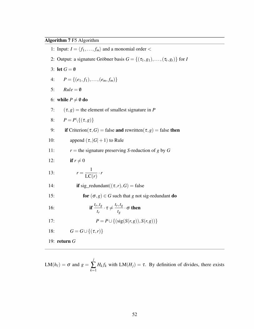
Algorithm 7 F5 Algorithm
1: Input: I = 〈 f1, . . . , fm〉 and a monomial order <
2: Output: a signature Gröbner basis G = {(τ1,g1), . . . ,(τt ,gt)} for I
3: let G = /0
4: P = {(e1, f1), . . . ,(em, fm)}
5: Rule = /0
6: while P 6= /0 do
7: (τ,g) = the element of smallest signature in P
8: P = P\{(τ,g)}
9: if Criterion(τ,G) = false and rewritten(τ,g) = false then
10: append (τ, |G|+1) to Rule
11: r = the signature preserving S-reduction of g by G
12: if r 6= 0
13: r =1
LC(r)· r
14: if sig_redundant((τ,r),G) = false
15: for (σ ,g) ∈ G such that g not sig-redundant do
16: iftr, tg
tr· τ 6=
tr, tgtg·σ then
17: P = P∪{(sig(S(r,g)),S(r,g))}
18: G = G∪{(τ,r)}
19: return G
LM(h`) = σ and g =j
∑k=1
Hk fk with LM(H j) = τ . By definition of divides, there exists
52
t ∈M such that t LM(g) = σ . Then
f = f −σ f`+σ f`
= f −σ f`+σ f`− t(g f`−g f`)
= f −σ f`+(σ − t LM(g)) f`− t(g−LM(g)) f`+ tj
∑k=1
( f`Hk) fk
Since t LM(g) = σ , we get
= f −σ f`− t(g−LM(g)) f`+ tj
∑k=1
( f`Hk) fk
=
(`
∑k=1
hk fk−LM(h`) f`
)(A)
− t(g−LM(g)) f`(B)
+ tj
∑k=1
( f`Hk) fk
Now, in (A) and (B), we have cancellation of LM(h`) f` and t LM(g) f`, respectively. That,along with the fact that k < ` for all k ∈ {1, . . . , j} in the last term means that we have notsatisfied the requirement in Definition 4.1.2 that (σ ,e`) be the smallest pair. Therefore, σe`is not the correct signature of f ! There is a smaller signature associated with it, and since weprogress through the algorithm in order of ascending signature, we have already consideredthis signature.
Also in line 9, rewritten(τ,g) tests if the polynomial was “rewritten” by a prior computa-tion by comparing it to a list of Rules.
Definition 4.2.2 (Adapted from Definition 10 of [6]). Rule is a list of rewritings for f if forevery (τ, `) ∈ Rule, where τ = sig(g`), there exists gi,g j ∈ G such that
(i) τ is the signature of S(gi,g j)
(ii) ` > i, j, and S(gi,g j) was reduced to g` in line 11 of Algorithm 7.
(iii) there exists (or P is scheduled to compute) a signature preserving S-representation ofS(gi,g j) such that h` = 1.
We add a new tuple to Rule each time we perform an S-reduction (line 11).
Definition 4.2.3. Given signatures σ = σ ′ei and τ = τ ′e j, we define signature divisibilityas τ | σ if j = i and τ ′ | σ ′.
53
Definition 4.2.4. Let S(gi,g j) = tgi − ug j, f = tgi,(τ, `) ∈ Rule, and (σ ,S(gi,g j)) ∈ P
without loss of generality σ = sig( f ). The rewritable criterion tests to see whether anS-reduction for S(gi,g j) can be avoided by checking if the following are true:
(i) τ | σ
(ii) ` > i, j
(iii) if (τ ′,k) ∈ Rule such that τ ′ | σ then k < `.
If all of these are true, rewritten(σ ,S(gi,g j)) returns True, and we say that (σ , f ) wasrewritten by (τ,g`).
Lemma 4.2.2 (Lemma 13 of [6]). Let f = tgi,(τ, `) ∈ Rule, and (σ , f ) be rewritten by
(τ, `). If the Algorithm 7 terminates with G, then there exist d,Hλ ∈ k[x1, . . . ,xn] with
λ ∈ {1, . . . , |G|} \{`} such that
f = dg`+ ∑gλ∈G\{g`}
Hλ gλ
where
(i) for all gλ ∈ G\{g`}, if Hλ 6= 0 then sig(LM(Hλ ) ·gλ )≺ t sig(gi) and
(ii) t sig(gi) is the signature of d sig(g`), meaning t sig(gi) = d sig(g`).
The proof of this is quite complicated and can be found in [6].In lines 12 and 13, if we did not compute a syzygy, we make the polynomial monic. The
reader will also notice that in line 14, we check whether sig_redundant((τ,h),G) is true ornot. This part of the algorithm is different from Faugére’s original F5 algorithm. It was firstdefined in [7] in the following way.
Definition 4.2.5 (Definition 10 of [7]). Let G be a signature Gröbner basis and (τ, f ) bean element we are considering adding to G. If there exists (σ ,g) ∈ G such that σ | τ andLM(g) | LM( f ), then (τ, f ) is signature-redundant to G, abbreviated sig-redundant.
Lemma 4.2.3 (Lemma 13 of [7]). If line 14 of Algorithm 7 finds sig_redundant((τ, f ),G))
to be true, the critical pairs associated with (τ, f ) already have signature preserving S-
representations or will after consideration of the pairs already in P.
Proof. By Definition 4.2.5, there exists (σ ,g) ∈ G such that σ | τ and LM(g) | LM( f ).Suppose σ = σ ′ei+1 and τ = τ ′ei+1. By definition of divides, there exists u ∈M such that
54
uLM(g) = LM( f ). If uσ ′ < τ ′, Line 11 did not compute a signature preserving S-reductionof S( f ,g), because g could reduce f further, a contradiction. Therefore uσ ′ ≥ τ ′.
Let t ∈M such that uσ ′ ≥ τ ′ = tσ ′, then LM( f ) = uLM(g)≥ t LM(g). The signatureµ = µ ′e j of s = f − tg is smaller that σ , so, by the method of ascending signature, thealgorithm has considered S-reductions for µ and smaller signatures. Therefore, (µ,s) has asignature preserving S-representation. We have already generated critical pairs for g since itis in the basis, so for any (ζ ,gi) ∈ G there exist u, t ∈M such that S( f ,gi) = u f − tgi. Bysubstitution, we have
S( f ,gi) = u f − tgi
= u(s+ tg)− tg,
whose S-reductions already have signature preserving S-representations or will after thealgorithm considers the pairs already in P.
Finally, we need a way to check if we have computed an actual Gröbner basis, for whichwe use the following characterization.
Theorem 4.2.4. (Theorem 9 of [7]) Suppose Gi = {g1, . . . ,gm}. Let τ1, . . . ,τ` be monomials
in M and p1, . . . , p` ∈ Ii+1 \{0} such that
G = {(σ1e j1 ,g1), . . . ,(σme jm ,gm)}∪{(ei+1, fi+1),(τ1ei+1, p1), . . . (τ`ei+1, p`)},
σe j = sig(g) for every (σe j,g) ∈ G, and for every (σei+1, p),(τe j,q) ∈ G one of the
following holds:
(i)(
tp,q
tp·σ)
ei+1 =
(tp,q
tq· τ)
e j, or
(ii)(
tp,q
tp·σ)
ei+1 �(
tp,q
tq· τ)
e j and(tp,q
tp·σei+1,S(p,q)
)has a signature preserving S-representation with respect to G.
Then Gi+1 = {g | (σe j,g) ∈ G where j ≤ i+1} is a Gröbner basis for Ii+1 with respect to
<.
Proof. By Theorem 4.1.1 and since Gi is a Gröbner basis of Ii, we know that for every pairp, q ∈Gi, S(p, q) has an S-representation with respect to Gi. To prove that Gi+1 is a Gröbnerbasis for Ii+1, we need only to show that the pairs p,q ∈ Gi+1 where at least p /∈ Gi also
have an S-representation. By hypothesis, if(
tp,q
tp·σ)
ei+1 �(
tp,q
tq· τ)
e j and j ≤ i+ 1,
55
(tp,q
tp·σei+1,S(p,q)
)has a signature preserving S-representation with respect to G. This
also means the pair p,q has an S-representation with respect to Gi+1 (see Remark 4.1.1).Order the remaining S-polynomials by ascending signature and choose the smallest
S(p,q) such that j ≤ i+ 1, (σei+1, p),(τe j,q) ∈ G, and(
tp,q
tp·σ)
ei+1 =
(tp,q
tq· τ)
e j.
WriteS(p,q) =
tp,q
tp· p−
tp,q
tq·q.
Then S(p,q) has a signature smaller than(
tp,q
tp·σ)
ei+1. Let h1, . . . ,h j ∈ k[x1, . . . ,xn] such
that
S(p,q) =j
∑k=1
hk fk
and LM(h j)e j = sig(S(p,q)). We see that each LM(hk)ek ≺(
tp,q
tp·σ)
ei+1, since either
k < i+1 or k = i+1 and LM(hk)<tp,q
tp·σ by Definition 4.1.2. Since S(p,q) has a smaller
signature than the signatures we have canceled, and since it was chosen as the smallest S-polynomial with canceling signatures, it must have a signature-preserving S-representation.
We can now proceed inductively: the next smallest S(p,q) with canceling signaturescan also be written with a smaller signature, and since all smaller signatures have signature-preserving S-representations (include the canceling pair we just considered), this pair mustalso have a signature-preserving S-representation.
Theorem 4.2.5 (Theorem 14 of [7]). Algorithm 7 terminates correctly.
Proof. Correctness: The only S-polynomials for which the algorithm does not computesignature preserving S-representations are those thrown out by lines 9, 12, 14, or 16.Lemmas 4.2.1 and 4.2.2 show that those thrown in line 9 have signature preserving S-representations when the algorithm terminates. Line 12 only removes syzygies as inAlgorithm 1. Lemma 4.2.3 shows that those thrown out by line 14 already have signaturepreserving S-representations. Finally, line 16 is one of the hypotheses of Theorem 4.2.4.Therefore, by Theorem 4.2.4, G = {g | g ∈ G} is a Gröbner basis.
Termination: Let M′ be the set of monomials in x1, . . . ,x2n. By Dickson’s Lemma(Corollary 1.3.6 of [14]), we know that M′ is Noetherian, or finitely generated. Any (σei,g)
added to G corresponds to an element of M′ in the following way
(σ ,LM(g)) =(
Πxαii ,Πxβi
i
)7→Πxαi
i Πxβin+i.
56
Let J be the M′-submodule generated by these (σ ,g). Now, suppose the algorithm adds(σ ,g) to G but J does not expand. Then there must exist (τ i,h) ∈ G such that τ | σ andLM(h) | LM(g), because if either of those were not true, J would have expanded. ByDefinition 4.2.5, (σei,g) is sig-redundant, so line 14 keeps it from generating new pairs.Therefore, each (σei,g) added to G either expands J or the algorithm prevents it fromcreating new pairs. Since M′ is Noetherian, this process can only repeat finitely many times,meaning the algorithm computes finitely many pairs. Therefore, Algorithm 7 terminates.
Now that we have defined the F5 algorithm, we will walk through Example 1.3.3 usingit.
4.2.1 Example of Gröbner basis computation with the F5 algorithm
Example 4.2.1. As before, let < be grevlex order and I = 〈x3−2xy,x2y−2y3+x〉. We willwalk through the F5 algorithm.
3: G = /0
4: P = {(e1, f1),(e2, f2)}
5: Rule = /0
Loop 1:
6: P 6= /0
7: Choose (e1, f1), since e1 is the smallest signature in P
8: P = {(e2, f2)}
9: Criterion(e1,G) = false and rewritten(e1, f1) = false, so we continue.
10: Rule = {(e1,1)}
11: r = f1 (It cannot be further reduced.)
12: r 6= 0
13: r is already monic.
14: G is empty, so we can skip lines 14 - 17.
18: G = {(e1,x3−2xy)}
57
Loop 2:
7: Choose (e2, f2)
8: P = /0
9: Criterion(e2,G) = false and rewritten(e2, f2) = false, so we continue.
10: Rule = {(e1,1),(e2,2)}
11: r = f2 (Again, it cannot be further reduced.)
12: r 6= 0
13: r is already monic.
14: sig_redundant((e2, f2),G))) = false
15: G only contains (e1,g1)
16: x · e2 6= y · e1
17: P = {(xe2,S(r,g1))}
18: G = G∪{(e2,x2y−2y3 + x)}
Loop 3:
7: Choose (xe2,S(g2,g1))
8: P = /0
We need to check rewritten(xe2,S(g2,g1)) against Rule = {(e1,1),(e2,2)}. Noticethat e2 | xe2 but `= j = 2, so it is not rewritten.
9: Criterion(xe2,G) = false and rewritten(xe2,S(g2,g1)) = false.
10: Rule = {(e1,1),(e2,2),(xe2,3)}
11: r =−2xy3 +2xy2 + x2
12: r 6= 0
13: r = xy3− xy2− 12x2
14: A quick inspection of G shows that r is not sig-redundant.
58
15: We look at both (e1,g1) and (e2,g2)
16: (e1,g1): x2 · xe2 6= y3 · e1
(e2,g2): x · xe2 6= y2 · e1
17: P = {(x3e2,S(r,g1)),(x2e2,S(r,g2))}
18: G = G∪{(xe2,xy3− xy2− 12x)}
Loop 4:
7: Choose (x2e2,S(g3,g2)) since x2e2 ≺ x3e2.
8: P = {(x3e2,S(g3,g1))}
We need to check (x2e2,S(g3,g2)) against Rule = {(e1,1),(e2,2),(xe2,3)}.
We see that e2 | x2e2 but `= i = 2. Also, xe2 | x2e2 but `= j = 3.
9: Criterion(x2e2,G) = false and rewritten(x2e2,g) = false
10: Rule = {(e1,1),(e2,2),(xe2,3),(x2e2,4)}
11: r = 2y5−2y4− xy2
12: r 6= 0
13: r = y5− y4− 12xy2
14: Although, e2 and xe2 divide x2e2, neither x3y nor xy3 divide y5, so r is not
sig-redundant.
15: We look at (e1,g1), (e2,g2), and (xe2,g3).
16: (e1,g1): x3 · x2e2 6= y5 · e1
(e2,g2): x2 · x2e2 6= y4 · e2
(xe2,g3): x · x2e2 6= y2 · xe2
17: P= {(x3e2,S(g3,g1)),(x5e2,S(r,g1)),(x4e2,S(r,g2)),(x3e2,S(r,g3))}
18: G = G∪{(x2e2,y5− y4− 12xy2)}
59
For each of the remaining elements in P, we see that Criterion(τ,G) = true, sinceLM(g1) = x3 | x3,x4,x5. This means that we have finished the computation and return
G = {(e1,x3−2xy),(e2,x2y−2y3 + x),(xe2,xy3− xy2− 12
x),(x2e2,y5− y4− 12
xy2)}.
We can check that this is in fact a Gröbner basis using the criteria of Theorem 4.2.4. It iseasy to see that any gi,g j ∈ G meet the second criterion, so we have a Gröbner basis.
Moreover, the polynomials in the final basis are exactly those we found in Example1.3.3, except with this algorithm, we were able to avoid all four of the reductions to zero wehad to compute using Buchberger’s algorithm.
60
Chapter 5
Dynamic F5 Algorithm
5.1 Introduction
In Chapter 3, we saw that dynamic algorithms for Gröbner basis computation typically yielda smaller basis than their static counterparts. In Chapter 4, we saw that the F5 algorithmutilizes signatures to avoid useless computations. One might wonder what would happenif we tried to create a dynamic F5 algorithm. Would that lead to a smaller Gröbner basisand avoid many useless computations? Another consideration is that, previously, we neededonly to ensure that the leading monomials of the basis elements remained unchanged ifthe order was changed. Now, we will also need to ensure that signatures of basis elementsremain unchanged as well. We will address both of these concerns in Section 5.2.
We have designed an algorithm that accomplishes both of these goals. We present thealgorithm in Section 4.2 and some computational results in Section 5.3. This algorithmuses a similar approach to previous dynamic algorithms for Gröbner basis computation. Inparticular, we use the Hilbert heuristic from [19] to choose a preferable leading monomialonce an S-reduction has occurred. We use the boundary vector method of [4] to removeincompatible leading monomials from our list of possibilities. We still implement F5defining procedures, including the rewritable criterion and Faugére’s criterion. We alsoimplement the sig-redundant criterion described in [6].
5.2 Dynamic F5 Algorithm
We present the main algorithm first, then follow up with discussion on some of the proceduresused. In Algorithm 8, we define the set of critical pairs in essentially the same way asAlgorithm 7; however, it is represented differently. In the static algorithm, we showed thecritical pairs as (τ,g) where g = S(gi,g j) and τ = sig(S(gi,g j)) for the gi,g j ∈ G that weused to find g. In this algorithm, we present a pair as (τ,(tgi,ug j)) where t =
tgi,g jtgi
and
u=tgi,g jtg j
. Clearly, S(gi,g j) = tgi−ug j, so we are representing the same elements in a slightly
modified format. We will assume without loss of generality that τ = sig(S(gi,g j)) = sig(tgi),and we know that τ = τ ′ev with τ ′ ∈M and v ∈ {1, . . . ,m}.
61
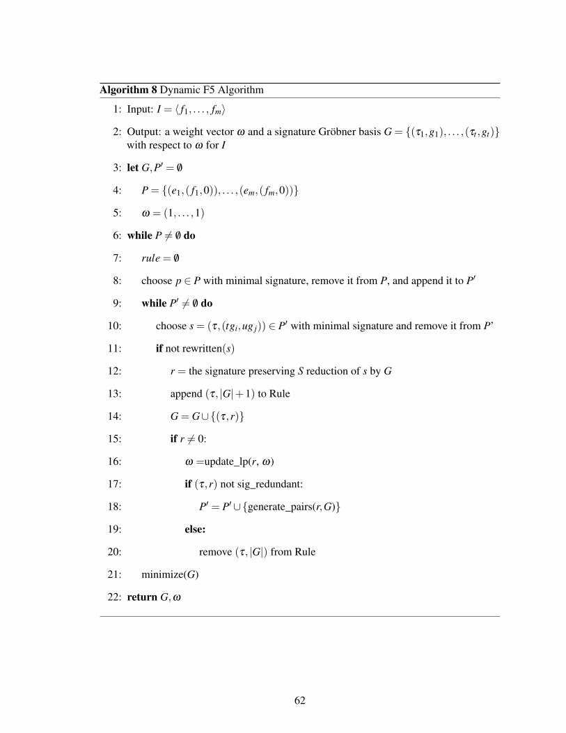
Algorithm 8 Dynamic F5 Algorithm
1: Input: I = 〈 f1, . . . , fm〉
2: Output: a weight vector ω and a signature Gröbner basis G = {(τ1,g1), . . . ,(τt ,gt)}with respect to ω for I
3: let G,P′ = /0
4: P = {(e1,( f1,0)), . . . ,(em,( fm,0))}
5: ω = (1, . . . ,1)
6: while P 6= /0 do
7: rule = /0
8: choose p ∈ P with minimal signature, remove it from P, and append it to P′
9: while P′ 6= /0 do
10: choose s = (τ,(tgi,ug j)) ∈ P′ with minimal signature and remove it from P’
11: if not rewritten(s)
12: r = the signature preserving S reduction of s by G
13: append (τ, |G|+1) to Rule
14: G = G∪{(τ,r)}
15: if r 6= 0:
16: ω =update_lp(r, ω)
17: if (τ,r) not sig_redundant:
18: P′ = P′∪{generate_pairs(r,G)}
19: else:
20: remove (τ, |G|) from Rule
21: minimize(G)
22: return G,ω
62
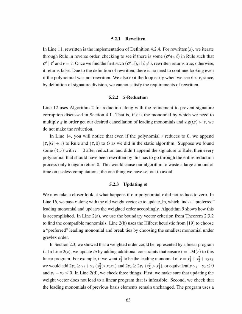
5.2.1 Rewritten
In Line 11, rewritten is the implementation of Definition 4.2.4. For rewritten(s), we iteratethrough Rule in reverse order, checking to see if there is some (σ ′ev, `) in Rule such thatσ ′ | τ ′ and v = v. Once we find the first such (σ ′, `), if ` 6= i, rewritten returns true; otherwise,it returns false. Due to the definition of rewritten, there is no need to continue looking evenif the polynomial was not rewritten. We also exit the loop early when we see v < v, since,by definition of signature division, we cannot satisfy the requirements of rewritten.
5.2.2 S-Reduction
Line 12 uses Algorithm 2 for reduction along with the refinement to prevent signaturecorruption discussed in Section 4.1. That is, if t is the monomial by which we need tomultiply g in order get our desired cancellation of leading monomials and sig(tg)� τ , wedo not make the reduction.
In Line 14, you will notice that even if the polynomial r reduces to 0, we append(τ, |G|+ 1) to Rule and (τ,0) to G as we did in the static algorithm. Suppose we foundsome (τ,r) with r = 0 after reduction and didn’t append the signature to Rule, then everypolynomial that should have been rewritten by this has to go through the entire reductionprocess only to again return 0. This would cause our algorithm to waste a large amount oftime on useless computations; the one thing we have set out to avoid.
5.2.3 Updating ω
We now take a closer look at what happens if our polynomial r did not reduce to zero. InLine 16, we pass r along with the old weight vector ω to update_lp, which finds a “preferred”leading monomial and updates the weighted order accordingly. Algorithm 9 shows how thisis accomplished. In Line 2(a), we use the boundary vector criterion from Theorem 2.3.2to find the compatible monomials. Line 2(b) uses the Hilbert heuristic from [19] to choosea “preferred” leading monomial and break ties by choosing the smallest monomial undergrevlex order.
In Section 2.3, we showed that a weighted order could be represented by a linear programL. In Line 2(c), we update ω by adding additional constraints that ensure t = LM(r) to thislinear program. For example, if we want x2
2 to be the leading monomial of r = x21+x2
2+x2x3,we would add 2y2≥ y2+y3 (x2
2 > x2x3) and 2y2≥ 2y1 (x22 > x2
1), or equivalently y3−y2≤ 0and y1− y2 ≤ 0. In Line 2(d), we check three things. First, we make sure that updating theweight vector does not lead to a linear program that is infeasible. Second, we check thatthe leading monomials of previous basis elements remain unchanged. The program uses a
63
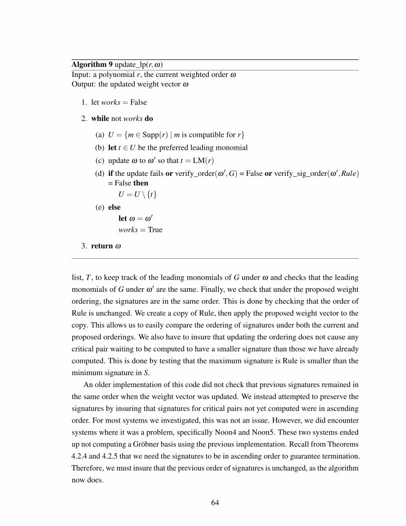
Algorithm 9 update_lp(r,ω)Input: a polynomial r, the current weighted order ω
Output: the updated weight vector ω
1. let works = False
2. while not works do
(a) U = {m ∈ Supp(r) | m is compatible for r}(b) let t ∈U be the preferred leading monomial
(c) update ω to ω ′ so that t = LM(r)
(d) if the update fails or verify_order(ω ′,G) = False or verify_sig_order(ω ′,Rule)= False then
U =U \{t}(e) else
let ω = ω ′
works = True
3. return ω
list, T , to keep track of the leading monomials of G under ω and checks that the leadingmonomials of G under ω ′ are the same. Finally, we check that under the proposed weightordering, the signatures are in the same order. This is done by checking that the order ofRule is unchanged. We create a copy of Rule, then apply the proposed weight vector to thecopy. This allows us to easily compare the ordering of signatures under both the current andproposed orderings. We also have to insure that updating the ordering does not cause anycritical pair waiting to be computed to have a smaller signature than those we have alreadycomputed. This is done by testing that the maximum signature is Rule is smaller than theminimum signature in S.
An older implementation of this code did not check that previous signatures remained inthe same order when the weight vector was updated. We instead attempted to preserve thesignatures by insuring that signatures for critical pairs not yet computed were in ascendingorder. For most systems we investigated, this was not an issue. However, we did encountersystems where it was a problem, specifically Noon4 and Noon5. These two systems endedup not computing a Gröbner basis using the previous implementation. Recall from Theorems4.2.4 and 4.2.5 that we need the signatures to be in ascending order to guarantee termination.Therefore, we must insure that the previous order of signatures is unchanged, as the algorithmnow does.
64
In one of our early implementations, if we had an infeasible linear program or anyprevious leading monomial changed, we removed t from U and tried again. We have sinceadded one additional step in an attempt to preserve our preferable leading monomial. If thecheck against T finds that one or more of the leading monomials has changed, we add newconstraints that undo this change. For example, suppose LMω(g) = x1x2 but LMω(g) = x0x2.We add y1y2 ≥ y0y2 to L then check to make sure the system is feasible and that we haven’tdisrupted any other leading monomials. We only attempt this refinement one time. If weare unable to find a feasible linear system for t that preserves previous leading monomials,we remove t from U and try again. Otherwise, we solve the new linear program, and thesolution becomes our updated ω ′.
Lemma 5.2.1. Algorithm 9 terminates correctly.
Proof. To show that the algorithm terminates, we only need to show that at some pointwe find works = True. Let t ′ = LM(r) under the current weighted order ω , then, certainly,t ′ ∈U . If we choose t ′ in Step 2(b), then the updated ω is exactly the current ω . We haveadded no constraints to the linear program, so we know it has a solution. It is obvious thatprior signatures and leading monomials remain unchanged, so works = True. We removeelements of U until we find a t that meets our needs, so we either find a t that is “morepreferable” than t ′ with works = True, or we end up with t ′.
To show correctness, we need to show that t = LM(r) under the updated ω , but that isexactly what Line 2(c) does.
5.2.4 Signature Redundant
Line 17 checks if (τ,r) is sig_redundant using Definition 4.2.5. In the static F5 algorithm,we had the freedom to check if the polynomial was signature redundant when we checked ifit was equal to 0. We only chose not to in that algorithm because we wanted to make thepolynomial monic first. In Algorithm 8, we do not have such freedom. Suppose we checkedfor signature redundancy before updating ω and found some (σ ,g) ∈ G where σ | τ andLM(g) | LM(r). One of two things could go wrong:
• If we choose a new leading monomial for r in update_lp, it is unlikely we will stillhave LM(g) | LM(r). This means we no longer have signature redundancy, and weend up not generating critical pairs that are necessary.
• Suppose we skip updating ω once we find a sig-redundant polynomial. It is possiblethat we have missed out on a “better” order, so we lose some of the benefits of adynamic algorithm.
65
5.2.5 Generating Critical Pairs
The only thing left to do is generate critical pairs. This part of the dynamic algorithm isexactly the same as in the static F5 algorithm. For any new pair (sig(S(r,g)),(tr,ug)), ifsig(tr) 6= sig(ug) and LM(gi) - sig(S(r,g)) for any gi ∈ G, then we add a new critical pairto P′. The second criterion is Faugére’s criterion from Definition 4.2.1.
5.2.6 Minimizing the Basis
For each Gi, we use Lemma 1.3.1 to remove any redundant polynomials from the basisbefore moving on. Line 19 does this by checking whether any leading monomials of thebasis elements are divisible by the leading monomial of any other basis element. If thereexists g j,gk ∈ Gi such that LM(g j) | LM(gk), we remove gk from Gi.
5.2.7 Correctness and Termination of Algorithm 8
In Section 5.1, we mentioned that we needed to also ensure that the signatures remainunchanged anytime we update ω . In order to do this, we need a special property ofsignatures.
Lemma 5.2.2 (Lemma 14 of [6] and Lemma 2 of [1]). Let Gi be a Gröbner basis of
Ii = 〈 f1, . . . , fm〉, f ∈ Gi, t,σ ∈M, and sig( f ) = σe j where j ≤ i. Then
(i) sig(t f ) = t sig( f ) or
(ii) there exists a syzygy h of Ii such that sig(h · f) = t sig( f ).
Proof. By Definition 4.1.2, there exist H1, . . . ,Hm ∈ k[x1, . . . ,xn] such that
f =m
∑k=1
Hk fk,
H j+1 = · · ·= Hm = 0, and LM(H j) = σ . Then
t f =j
∑k=1
tHk fk.
If sig(t f ) = t LM(H j) = t sig( f ), we have (i). Otherwise, sig(t f ) ≺ t LM(H j). Let v ∈{1, . . . ,m}, τ ∈M such that τev = sig(t f ). Again, by Definition 4.1.2, there exist h′1, . . . ,h
′m ∈
k[x1, . . . ,xn] such that
t f =m
∑k=1
h′k fk,
66
h′v+1 = · · · = h′m = 0, and LM(h′v) = τ . Since τev ≺ σe j, we know that v ≤ j ≤ i. Leth = tH−h′, meaning
hk =
tHk−h′k, 1≤ k ≤ vtHk, v < k ≤ j0, j < k ≤ m
Obviously, t f − t f = 0 which gives us
0 = t f − t f
=m
∑k=1
tHk fk−m
∑k=1
h′k fk
=m
∑k=1
(tHk−h′k) fk
=m
∑k=1
hk fk.
We know that h 6= 0, since tH j 6= 0 and h′j = 0 meaning hk = tH j 6= 0. Therefore, h is asyzygy of Ii, and, by Definition 4.1.2, sig(h · f) = t LM(Hk) = t sig( f ), so we have (ii).
Now, we can show that our signature remain unchanged upon updating ω .
Lemma 5.2.3. If (τ,g`) ∈ G, then τ = sig(g`) for any ω returned by Algorithm 9.
Proof. Suppose (τ,g`)∈G and ω is a weighted order returned by Algorithm 9. Let τ = τ ′ek
for some k ∈ {1, . . . ,m}. If τ ′ = 1, then we are done. Otherwise, τ ′ek = sig(S(gi,g j)) forsome i, j < ` such that gi,g j 6= 0. We know by our method of adding critical pairs that
sig(
tgi,g j
tgi
·gi
)6= sig
(tgi,g j
tg j
·g j
). This means that
sig(S(gi,g j)) = sig(
tgi,g j
tgi
·gi
)or
sig(S(gi,g j)) = sig(
tgi,g j
tg j
·g j
).
Without loss of generality, suppose we have sig(S(gi,g j)) = sig(
tgi,g j
tgi
·gi
). Since gi 6= 0
and by Lemma 5.2.2,
τ = sig(g`)
= sig(S(gi,g j))
= sig(
tgi,g j
tgi
·gi
)=
tgi,g j
tgi
· sig(gi).
67
Now, suppose sig(gi) = σ ′ek. By the same logic, σ ′ek = sig
(tgi,g j
tgi
·gi
)for some gi,g j ∈G
with gi,g j 6= 0, then
τ = sig(g`)
=tgi,g j
tgi
· sig
(tgi,g j
tgi
·gi
)
=tgi,g j
tgi
tgi,g j
tgi
· sig(gi).
We can repeat the same process until we have reached a gk that is the S-reduction of thegenerator fk, in which case we have (
Πtgi,g j
tgi
)· ek.
Notice that every element in the product is the least common multiple of two leadingmonomials divided by another leading monomial, all of which belong to prior elements of G.We already know that these are unchanged, as we checked them in verify_order. Therefore,τ remains unchanged and τ = sig(g`).
Theorem 5.2.4. Algorithm 8 terminates correctly in a finite number of steps with a signature
Gröbner basis for I under a weighted order ω .
Proof. By choosing minimal elements from our list of critical pairs, the criteria used togenerate critical pairs, and Lemma 5.2.3, we have shown that we proceed by ascendingsignature. Since no other major elements from Algorithm 7 have changed, Theorem 4.2.5applies.
Now that we have shown our algorithm works, let’s see how it actually performs.
5.3 Results
In order to check that we have computed a Gröbner basis, we remove the signatures fromthe output then check whether the polynomials satisfy Theorem 1.3.2, that is, we checkthat all distinct pairs reduce to zero. The Sage source code can be found in Appendix A.We use object-oriented programming to create classes for signatures, signed polynomials,and critical pairs. The code then follows closely with the pseudo-code seen throughout thiswork.
68
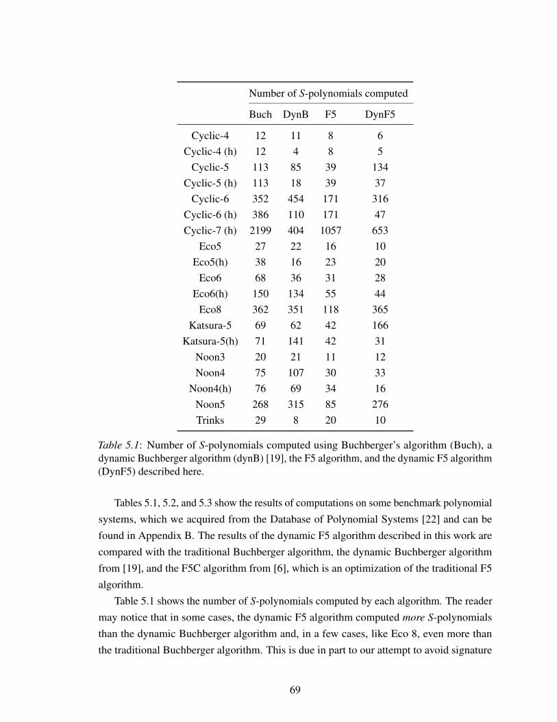
Number of S-polynomials computed
Buch DynB F5 DynF5
Cyclic-4 12 11 8 6Cyclic-4 (h) 12 4 8 5
Cyclic-5 113 85 39 134Cyclic-5 (h) 113 18 39 37
Cyclic-6 352 454 171 316Cyclic-6 (h) 386 110 171 47Cyclic-7 (h) 2199 404 1057 653
Eco5 27 22 16 10Eco5(h) 38 16 23 20
Eco6 68 36 31 28Eco6(h) 150 134 55 44
Eco8 362 351 118 365Katsura-5 69 62 42 166
Katsura-5(h) 71 141 42 31Noon3 20 21 11 12Noon4 75 107 30 33
Noon4(h) 76 69 34 16Noon5 268 315 85 276Trinks 29 8 20 10
Table 5.1: Number of S-polynomials computed using Buchberger’s algorithm (Buch), adynamic Buchberger algorithm (dynB) [19], the F5 algorithm, and the dynamic F5 algorithm(DynF5) described here.
Tables 5.1, 5.2, and 5.3 show the results of computations on some benchmark polynomialsystems, which we acquired from the Database of Polynomial Systems [22] and can befound in Appendix B. The results of the dynamic F5 algorithm described in this work arecompared with the traditional Buchberger algorithm, the dynamic Buchberger algorithmfrom [19], and the F5C algorithm from [6], which is an optimization of the traditional F5algorithm.
Table 5.1 shows the number of S-polynomials computed by each algorithm. The readermay notice that in some cases, the dynamic F5 algorithm computed more S-polynomialsthan the dynamic Buchberger algorithm and, in a few cases, like Eco 8, even more thanthe traditional Buchberger algorithm. This is due in part to our attempt to avoid signature
69
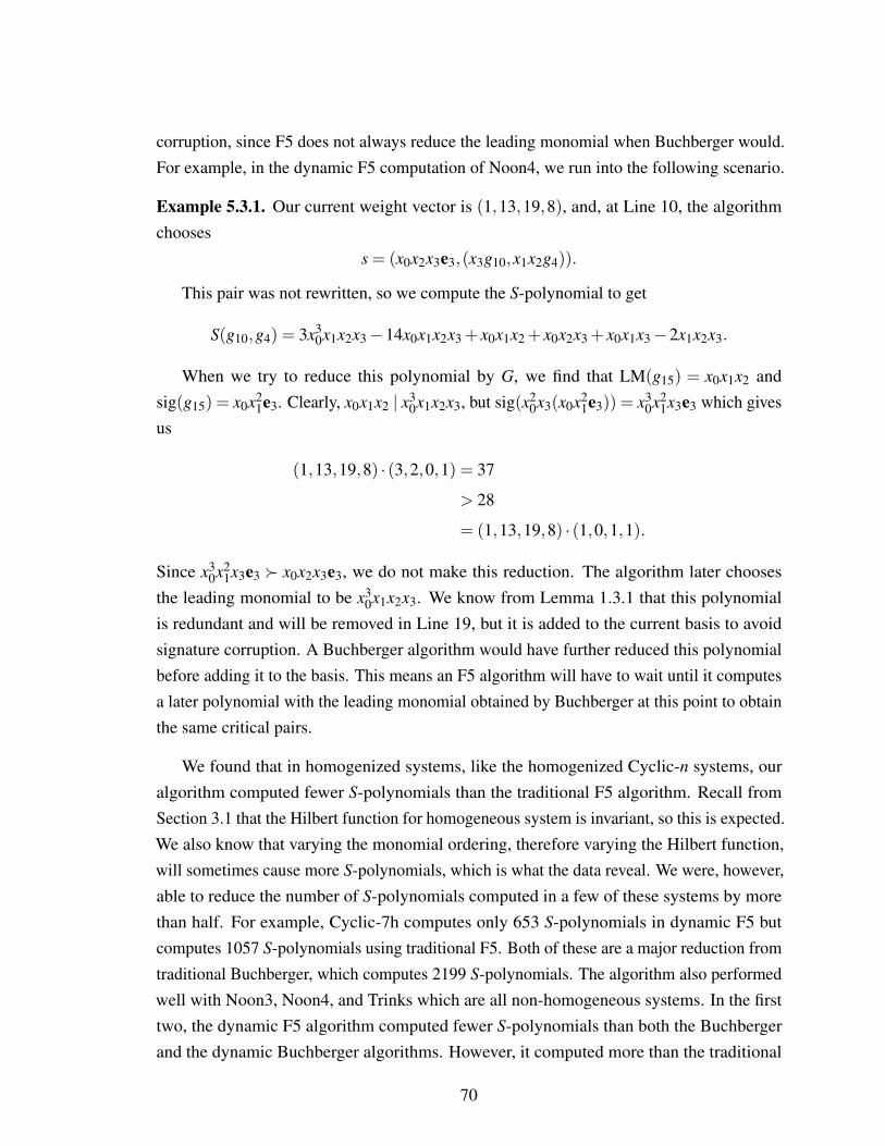
corruption, since F5 does not always reduce the leading monomial when Buchberger would.For example, in the dynamic F5 computation of Noon4, we run into the following scenario.
Example 5.3.1. Our current weight vector is (1,13,19,8), and, at Line 10, the algorithmchooses
s = (x0x2x3e3,(x3g10,x1x2g4)).
This pair was not rewritten, so we compute the S-polynomial to get
S(g10,g4) = 3x30x1x2x3−14x0x1x2x3 + x0x1x2 + x0x2x3 + x0x1x3−2x1x2x3.
When we try to reduce this polynomial by G, we find that LM(g15) = x0x1x2 andsig(g15) = x0x2
1e3. Clearly, x0x1x2 | x30x1x2x3, but sig(x2
0x3(x0x21e3)) = x3
0x21x3e3 which gives
us
(1,13,19,8) · (3,2,0,1) = 37
> 28
= (1,13,19,8) · (1,0,1,1).
Since x30x2
1x3e3 � x0x2x3e3, we do not make this reduction. The algorithm later choosesthe leading monomial to be x3
0x1x2x3. We know from Lemma 1.3.1 that this polynomialis redundant and will be removed in Line 19, but it is added to the current basis to avoidsignature corruption. A Buchberger algorithm would have further reduced this polynomialbefore adding it to the basis. This means an F5 algorithm will have to wait until it computesa later polynomial with the leading monomial obtained by Buchberger at this point to obtainthe same critical pairs.
We found that in homogenized systems, like the homogenized Cyclic-n systems, ouralgorithm computed fewer S-polynomials than the traditional F5 algorithm. Recall fromSection 3.1 that the Hilbert function for homogeneous system is invariant, so this is expected.We also know that varying the monomial ordering, therefore varying the Hilbert function,will sometimes cause more S-polynomials, which is what the data reveal. We were, however,able to reduce the number of S-polynomials computed in a few of these systems by morethan half. For example, Cyclic-7h computes only 653 S-polynomials in dynamic F5 butcomputes 1057 S-polynomials using traditional F5. Both of these are a major reduction fromtraditional Buchberger, which computes 2199 S-polynomials. The algorithm also performedwell with Noon3, Noon4, and Trinks which are all non-homogeneous systems. In the firsttwo, the dynamic F5 algorithm computed fewer S-polynomials than both the Buchbergerand the dynamic Buchberger algorithms. However, it computed more than the traditional
70
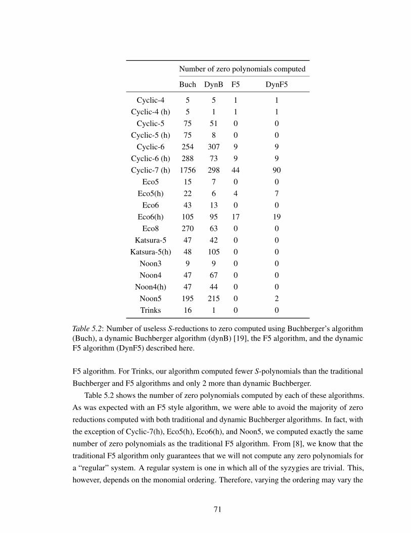
Number of zero polynomials computed
Buch DynB F5 DynF5
Cyclic-4 5 5 1 1Cyclic-4 (h) 5 1 1 1
Cyclic-5 75 51 0 0Cyclic-5 (h) 75 8 0 0
Cyclic-6 254 307 9 9Cyclic-6 (h) 288 73 9 9Cyclic-7 (h) 1756 298 44 90
Eco5 15 7 0 0Eco5(h) 22 6 4 7
Eco6 43 13 0 0Eco6(h) 105 95 17 19
Eco8 270 63 0 0Katsura-5 47 42 0 0
Katsura-5(h) 48 105 0 0Noon3 9 9 0 0Noon4 47 67 0 0
Noon4(h) 47 44 0 0Noon5 195 215 0 2Trinks 16 1 0 0
Table 5.2: Number of useless S-reductions to zero computed using Buchberger’s algorithm(Buch), a dynamic Buchberger algorithm (dynB) [19], the F5 algorithm, and the dynamicF5 algorithm (DynF5) described here.
F5 algorithm. For Trinks, our algorithm computed fewer S-polynomials than the traditionalBuchberger and F5 algorithms and only 2 more than dynamic Buchberger.
Table 5.2 shows the number of zero polynomials computed by each of these algorithms.As was expected with an F5 style algorithm, we were able to avoid the majority of zeroreductions computed with both traditional and dynamic Buchberger algorithms. In fact, withthe exception of Cyclic-7(h), Eco5(h), Eco6(h), and Noon5, we computed exactly the samenumber of zero polynomials as the traditional F5 algorithm. From [8], we know that thetraditional F5 algorithm only guarantees that we will not compute any zero polynomials fora “regular” system. A regular system is one in which all of the syzygies are trivial. This,however, depends on the monomial ordering. Therefore, varying the ordering may vary the
71
Final basis size |G|
Buch DynB F5 DynF5
Cyclic-4 7 7 7 5Cyclic-4 (h) 7 4 7 4
Cyclic-5 20 13 20 17Cyclic-5 (h) 38 11 38 22
Cyclic-6 44 21 44 19Cyclic-6 (h) 98 38 98 28Cyclic-7 (h) 443 107 443 110
Eco5 11 6 11 9Eco5(h) 15 9 15 12
Eco6 18 10 18 11Eco6(h) 44 39 28 19
Eco8 59 12 59 12Katsura-5 22 20 22 11
Katsura-5(h) 22 36 22 24Noon3 11 8 11 11Noon4 28 21 28 26
Noon4(h) 28 25 28 15Noon5 72 53 72 53Trinks 13 8 13 9
Table 5.3: Size of the Gröbner basis computing using Buchberger’s algorithm (Buch), adynamic Buchberger algorithm (dynB) [19], the F5 algorithm, and the dynamic F5 algorithm(DynF5) described here.
number of zero polynomials computed. This helps to explain why we compute more zeropolynomials than the traditional F5 algorithm in these four systems.
Table 5.3 compares the final sizes of the Gröbner bases computed. We remind the readerthat the algorithm computes a minimal Gröbner basis, so the final basis size representsthe number of S-polynomials computed minus not only the number of zero polynomialscomputed but also the elements of G whose leading monomials were divisible by anotherleading monomial of the basis. With the exception of Noon3 and Katsura-5(h), the dynamicF5 algorithm consistently returns a smaller basis than traditional F5, as we expected froma dynamic approach. We were happy to find that dynamic F5 also outperformed dynamicBuchberger in many cases. For example, Cyclic-6h had a final basis size of 28 polynomials
72
using our dynamic F5 algorithm, while the dynamic Buchberger algorithm had a finalbasis with 38 polynomials. For this same system, both the traditional Buchberger and thetraditional F5 algorithms returned a Gröbner basis with 98 polynomials. In many caseswhere our algorithm did not do better than dynamic Buchberger, it was not far behind.For instance, our dynamic F5 algorithm returned a basis of 110 polynomials for Cyclic-7hcompared to 107 polynomials using dynamic Buchberger. Even better, our basis is less thanone-fourth of the size of the bases computed by the traditional Buchberger and traditionalF5 algorithms, both having 443 polynomials.
Overall, the dynamic F5 algorithm outperforms its static counterpart. Although, weoccasionally compute more zero polynomials than traditional F5, we still reap the benefitsof avoiding many of the reductions to zero performed by Buchberger style algorithms. Wewere also generally able to compute fewer S-polynomials and still achieve smaller basissizes than both traditional Buchberger and traditional F5. In these ways, the algorithmperforms exactly as one would expect. It avoids reductions to zero as much as possiblewhile also minimizing the number of polynomials in the final basis.
5.4 Future Work
Table 5.4 shows the timings for running our dynamic F5 algorithm compared to a traditionalF5 algorithm. The times were obtained by running the code in Appendix A in an instanceof CoCalc at https://bagheera.usm.edu/. This page runs Sage version 8.9 [21] on a 24-coreIntel Xeon X5690 @3.47 GHz with 64 GB memory using Ubuntu 7.4.0 with the 4.15.0-74-generic Linux kernel. The times for the static algorithm were obtained after removingany lines of code that make the algorithm dynamic, such as updating the linear program.All times are an average of the times obtained by three full computations. We see that inthe larger homogeneous Cyclic-n systems, the dynamic version ran faster than this staticversion. This is due to there being fewer S-polynomials to compute when working with thefinal generator. The dynamic algorithm chooses hn to be the leading monomial for fn in anyCyclic-n(h) system, because it has the best Hilbert data. Since hn is relatively prime to any
other leading monomial in the basis, there are no additional critical pairs to add at this point,so the algorithm terminates.
For any other system, we see that our dynamic F5 algorithm comes with a high computa-tional cost. This is due in part to algorithm’s need to preserve signature order. As mentionedin Section 5.2.3, we sometimes do not choose the leading monomial with the best Hilbertdata, because it would corrupt the order of the signatures. This means that we choose one ofthe “runner ups.” From Section 3.1, we know that choosing the leading monomial with the
73
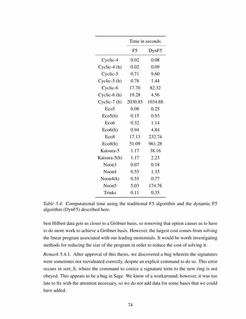
Time in seconds
F5 DynF5
Cyclic-4 0.02 0.08Cyclic-4 (h) 0.02 0.09
Cyclic-5 0.71 9.60Cyclic-5 (h) 0.78 1.44
Cyclic-6 17.70 82.32Cyclic-6 (h) 19.28 4.56Cyclic-7 (h) 2030.85 1034.88
Eco5 0.08 0.25Eco5(h) 0.15 0.93
Eco6 0.32 1.14Eco6(h) 0.94 4.84
Eco8 17.13 232.74Eco8(h) 51.09 961.28
Katsura-5 1.17 38.16Katsura-5(h) 1.17 2.23
Noon3 0.07 0.18Noon4 0.55 1.33
Noon4(h) 0.55 0.77Noon5 5.03 174.76Trinks 0.11 0.35
Table 5.4: Computational time using the traditional F5 algorithm and the dynamic F5algorithm (DynF5) described here.
best Hilbert data gets us closer to a Gröbner basis, so removing that option causes us to haveto do more work to achieve a Gröbner basis. However, the largest cost comes from solvingthe linear program associated with our leading monomials. It would be worth investigatingmethods for reducing the size of the program in order to reduce the cost of solving it.
Remark 5.4.1. After approval of this thesis, we discovered a bug wherein the signatureswere sometimes not reevaluated correctly, despite an explicit command to do so. This erroroccurs in sort_S, where the command to coerce a signature term to the new ring is notobeyed. This appears to be a bug in Sage. We know of a workaround; however, it was toolate to fix with the attention necessary, so we do not add data for some bases that we couldhave added.
74
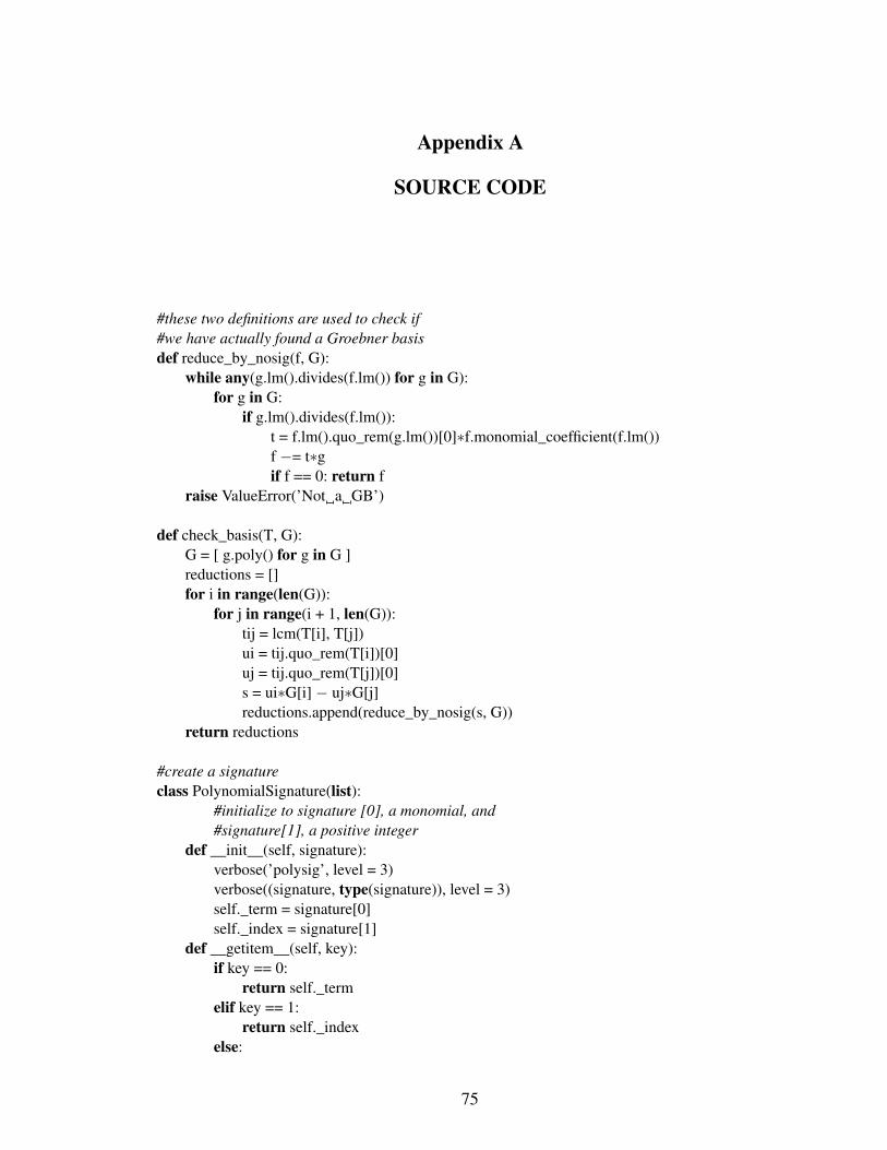
Appendix A
SOURCE CODE
#these two definitions are used to check if#we have actually found a Groebner basisdef reduce_by_nosig(f, G):
while any(g.lm().divides(f.lm()) for g in G):for g in G:
if g.lm().divides(f.lm()):t = f.lm().quo_rem(g.lm())[0]∗f.monomial_coefficient(f.lm())f −= t∗gif f == 0: return f
raise ValueError(’Not a GB’)
def check_basis(T, G):G = [ g.poly() for g in G ]reductions = []for i in range(len(G)):
for j in range(i + 1, len(G)):tij = lcm(T[i], T[j])ui = tij.quo_rem(T[i])[0]uj = tij.quo_rem(T[j])[0]s = ui∗G[i] − uj∗G[j]reductions.append(reduce_by_nosig(s, G))
return reductions
#create a signatureclass PolynomialSignature(list):
#initialize to signature [0], a monomial, and#signature[1], a positive integer
def __init__(self, signature):verbose(’polysig’, level = 3)verbose((signature, type(signature)), level = 3)self._term = signature[0]self._index = signature[1]
def __getitem__(self, key):if key == 0:
return self._termelif key == 1:
return self._indexelse:
75
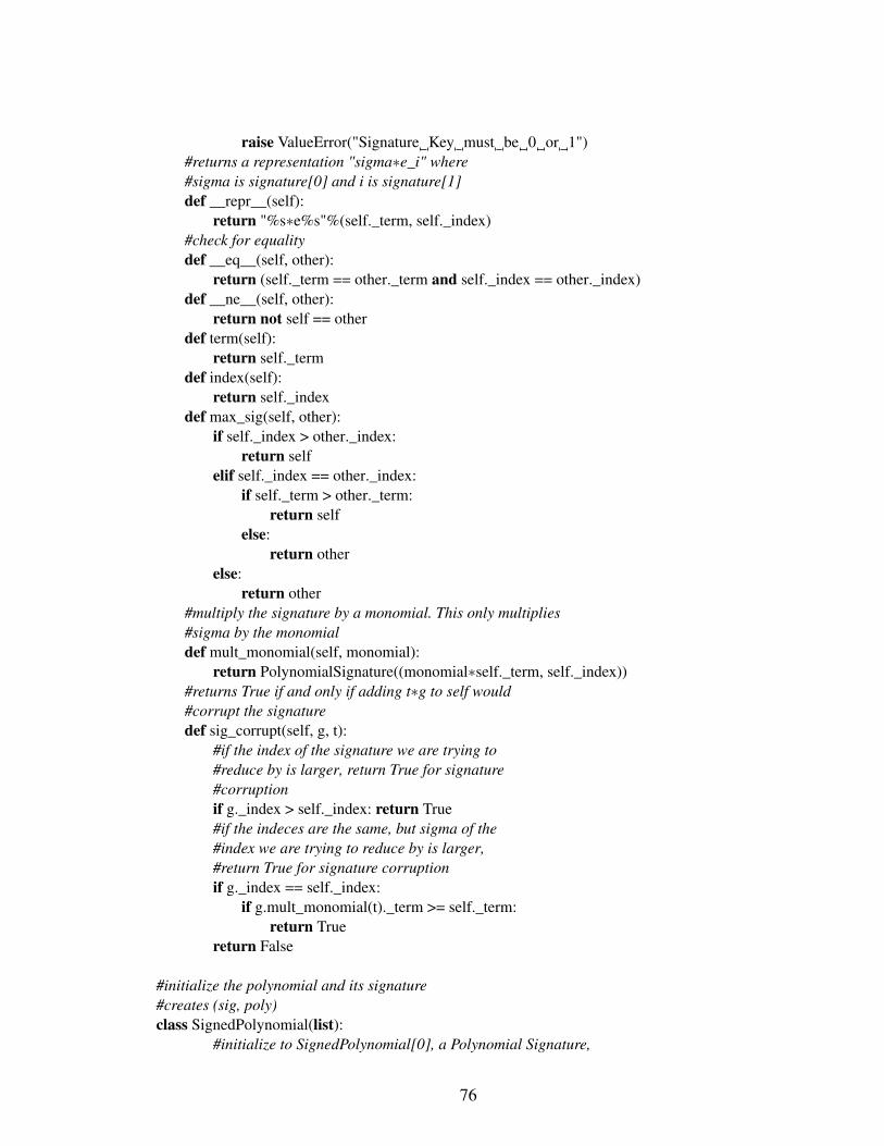
raise ValueError("Signature Key must be 0 or 1")#returns a representation "sigma∗e_i" where#sigma is signature[0] and i is signature[1]def __repr__(self):
return "%s∗e%s"%(self._term, self._index)#check for equalitydef __eq__(self, other):
return (self._term == other._term and self._index == other._index)def __ne__(self, other):
return not self == otherdef term(self):
return self._termdef index(self):
return self._indexdef max_sig(self, other):
if self._index > other._index:return self
elif self._index == other._index:if self._term > other._term:
return selfelse:
return otherelse:
return other#multiply the signature by a monomial. This only multiplies#sigma by the monomialdef mult_monomial(self, monomial):
return PolynomialSignature((monomial∗self._term, self._index))#returns True if and only if adding t∗g to self would#corrupt the signaturedef sig_corrupt(self, g, t):
#if the index of the signature we are trying to#reduce by is larger, return True for signature#corruptionif g._index > self._index: return True#if the indeces are the same, but sigma of the#index we are trying to reduce by is larger,#return True for signature corruptionif g._index == self._index:
if g.mult_monomial(t)._term >= self._term:return True
return False
#initialize the polynomial and its signature#creates (sig, poly)class SignedPolynomial(list):
#initialize to SignedPolynomial[0], a Polynomial Signature,
76
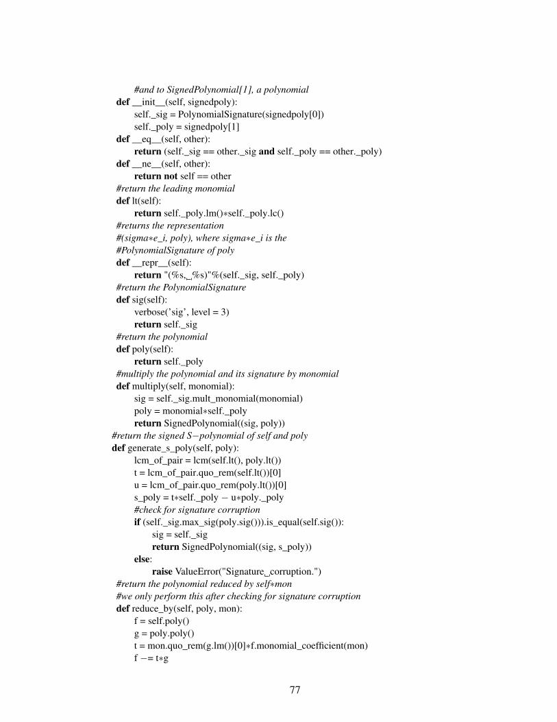
#and to SignedPolynomial[1], a polynomialdef __init__(self, signedpoly):
self._sig = PolynomialSignature(signedpoly[0])self._poly = signedpoly[1]
def __eq__(self, other):return (self._sig == other._sig and self._poly == other._poly)
def __ne__(self, other):return not self == other
#return the leading monomialdef lt(self):
return self._poly.lm()∗self._poly.lc()#returns the representation#(sigma∗e_i, poly), where sigma∗e_i is the#PolynomialSignature of polydef __repr__(self):
return "(%s, %s)"%(self._sig, self._poly)#return the PolynomialSignaturedef sig(self):
verbose(’sig’, level = 3)return self._sig
#return the polynomialdef poly(self):
return self._poly#multiply the polynomial and its signature by monomialdef multiply(self, monomial):
sig = self._sig.mult_monomial(monomial)poly = monomial∗self._polyreturn SignedPolynomial((sig, poly))
#return the signed S−polynomial of self and polydef generate_s_poly(self, poly):
lcm_of_pair = lcm(self.lt(), poly.lt())t = lcm_of_pair.quo_rem(self.lt())[0]u = lcm_of_pair.quo_rem(poly.lt())[0]s_poly = t∗self._poly − u∗poly._poly#check for signature corruptionif (self._sig.max_sig(poly.sig())).is_equal(self.sig()):
sig = self._sigreturn SignedPolynomial((sig, s_poly))
else:raise ValueError("Signature corruption.")
#return the polynomial reduced by self∗mon#we only perform this after checking for signature corruptiondef reduce_by(self, poly, mon):
f = self.poly()g = poly.poly()t = mon.quo_rem(g.lm())[0]∗f.monomial_coefficient(mon)f −= t∗g
77
self._poly = freturn self
#a class for critical pairs of signed polynomialsclass Pair(list):
#initialize to Pair[0], a PolynomialSignature, Pair[1], the#first SignedPolynomial in the critical pair, and to Pair[2],#the second SignedPolynomial in the critical pair
def __init__(self, pair):self._sig = PolynomialSignature(pair[0])self._poly1 = pair[1]self._poly2 = pair[2]
#represent the critical pair as "(sigma∗e_i, f, g)", where#sigma∗e_i is the PolynomialSignature of the critical pair,#f is the first polynomial, and g is the seconddef __repr__(self):
return "(%s, %s, %s)"%(self._sig, self._poly1, self._poly2)#return the signature of the critical pairdef sig(self):
verbose(’sig’, level = 3)return self._sig
#return the first polynomialdef poly1(self):
return self._poly1#return the second polynomialdef poly2(self):
return self._poly2def __eq__(self, other):
return (self._sig == other._sig and self._poly1[0] == other._poly1[0] \and self._poly1[1] == other._poly1[1] and self._poly2[0] == \other._poly2[0] and self._poly2[1] == other._poly2[1] )
def __ne__(self, other):return not self == other
#initialize a polynomial ring and return the ringdef initialize_ring(vars, ring):
if type(vars) == Integer:n = varsR = PolynomialRing(ring, ’x’, n)
else:R = PolynomialRing(ring, vars)
R.inject_variables()return R
#initialize the ideal and return the ring R, the ideal I,#the sorted generators F, the ring generators X, the weight#vector lp, and Y, a list of variables for the linear program
78
def initialize_ideal(polys, homogenize = False):R = polys[0].parent()if (homogenize):
I = R.ideal(polys).homogenize()R = I.ring()R.inject_variables()
else:I = R.ideal(polys)
F = list(I.gens())F.sort(key = lambda f: f.lm())for i in range(len(F)):
F[i] = SignedPolynomial(((R(1), i), F[i]))#F keeps up with the signatures and their corresponding polynomials#here, we are just declaring the original signatures f_1 −> (1∗e_1, f_1), etc.
X = I.ring().gens()lp, Y = initialize_lp(X, homogenize)return R, I, F, X, lp, Y
#initialize the linear program to a vector of ones#return this weight vector lp and Y, a list of variables for the#linear program#to be used in solving the linear programdef initialize_lp(X, homogenize = False):
lp = MixedIntegerLinearProgram(solver=’ppl’, maximization=False)Y = [ lp[i] for i in range(len(X)) ]for y in Y:
lp.set_integer(y)lp.add_constraint(y >= 1)
lp.set_objective(sum(y for y in Y))lp.solve()return lp, Y
#update lp based on new lm and return the new weight vectordef update_lp(f, lp, Y, T, X, R, G, S, trace, homogenize = False):
i = 0poly = fworks = Falsebad_t = Falselp_temp = copy(lp)lp_temp.solve()pp_old = 1while not works:
lp_new = copy(lp_temp)if bad_t == True:
U = [ u for u in U if u[0] != t ]else: U = compatible_pps(poly, lp_temp, Y)#if there are no monomials to compare, exit the loop
79
if len(U) == 1: return lp#otherwise, use the hilbert heuristic to find the#’best’ lmt = preferred_pp(T, [u[0] for u in U], R)a = t.exponents(as_ETuples=False)[0]new_expr = sum(a[i]∗Y[i] for i in range(len(a)))#make it the leading monomialfor u in [ v[0] for v in U ]:
if u != t:b = u.exponents(as_ETuples=False)[0]lp_new.add_constraint(new_expr >= sum(b[i]∗Y[i] for \
i in range(len(b))) + 1)try:
lp_new.solve()except:
#if updating the lp creates an infeasible system,#remove t from the optionsbad_t = Truecontinue
#insure that the signatures remained in the same order AND#the prior leading monomials remain unchangedif verify_signature_order(R, lp_temp, lp_new, Y, S, trace):
T_temp = copy(T)T_temp.append(t)works, lp_temp = verify_order(T_temp, G, R, lp_temp, lp_new, Y, X)pp_old = tbad_t = False
else:bad_t = Truecontinue
lp_temp.solve()return lp_temp
#return a matrix order with weight vector v and#grevlex to break tiesdef matrix_order(v, homogenize = False):
if homogenize:vlen = len(v) − 1
else:vlen = len(v)
A = matrix(ZZ, vlen, vlen)for i in range(vlen):
A[0,i] = v[i]for i in range(1,vlen):
for j in range(vlen−i):A[i,j] = 1
return TermOrder(A)
80
#returns the monomials of f that are compatible for f#lp tells us our current weight vector and Y is#a list of variables for the linear programdef compatible_pps(f, lp, Y):
result = [(f.lm(),lp.get_values(Y))]TOs = list(ray.vector() for ray in lp.polyhedron().rays())# test every monomial of ffor t in f.monomials()[1:]:
b = vector(t.exponents()[0]) # exponent vectorfor v in TOs:
success = True # innocent until proven guilty# test against every other monomial in ffor u in result:
if v ∗ b <= v ∗ vector(u[0].exponents()[0]):# give up on this ray; try anothersuccess = Falsebreak
if success:# we’ll add both t and a "certificate" that t can leadresult.append((t,v))# no point in remaining in the ray loop, since we’ve found a#winner for tbreak
return result
#apply the new monomial order and return the current basis under the#new weight ordering G, the updated ring R2, and the updated generators Fdef redefine_vals(lp, Y, R, G, F):
TO = matrix_order(lp.get_values(Y))R2 = R.change_ring(order=TO)#reorder polys in G according to new weight vectorG = [ SignedPolynomial(((R2(g.sig().term()), g.sig().index()), \
R2(g.poly()))) for g in G ]#reorder polys in F according to new weight vectorF = [ SignedPolynomial(((R2(f.sig().term()), f.sig().index()), \
R2(f.poly()))) for f in F ]if G[−1].poly() != 0:
#insure that the lc is 1if G[−1].poly().coefficient(G[−1].poly().lm()) != 1:
G[−1] = SignedPolynomial(((G[−1].sig().term(), G[−1].sig().index()), \G[−1].poly().quo_rem(G[−1].poly().coefficient(G[−1].poly().lm()))[0]))
return G, R2, F
# return the leading monomial that is "best" using the#hilbert heuristic. T is old basis’s lms, U is list of compatible#monomials to test
81
def preferred_pp(T, U, R):u0 = U[0]V = T + [u0]#create ideals with prior lms and the new optionshp = R.ideal(V).hilbert_polynomial(algorithm=’singular’)hn = R.ideal(V).hilbert_numerator(algorithm=’singular’)result = u0for u in U[1:]:
V = T + [u]hp2 = R.ideal(V).hilbert_polynomial(algorithm=’singular’)hn2 = R.ideal(V).hilbert_numerator(algorithm=’singular’)if hilbert_cmp((result,hp,hn),(u,hp2,hn2)) > 0:
result, hp, hn = u, hp2, hn2return result
#return a negative integer if H1 is preferable to H2,#a positve integer if H2 is preferable, and 0 if H1 and#H2 are the same. H1 and H2 represent the Hilbert numerator#and Hilbert polynomial for two choices of leading monomialsdef hilbert_cmp(H1, H2):
hpdiff = H1[1] − H2[1]#if the hilbert polynomial is smallest, choose as#preferred lmif hpdiff != 0:
result = hpdiff.leading_coefficient()#otherwise compare the hilbert numeratorselse:
hndiff = (H1[2] − H2[2]).coefficients(sparse=False)hndiff.reverse()while len(hndiff) > 0 and hndiff[0] == 0:
hndiff = hndiff[1:]if len(hndiff) == 0:
#if the Hilbert data is the same, choose the#monomial that is smaller under the monomial order#−1 will choose the monomial associated with H1,#1 will choose the monomial associated with H2,#0 means they have the same weighted degree and#defaults to the monomial associated with H1
if H1[0] < H2[0]: result = −1elif H1[0] > H2[0]: result = 1else: result = 0
else:#choose the monomial associated with the smallest#trailing term of the Hilbert numerator
result = hndiff[0]return result
82
#return a list of "critical pairs" for the generatorsdef generate_first_pairs(F):
#create pairs associated with zero for the initial polynomials#so we can add f_1, f_2, etc to the basis without an S−polyP = []S = []for i in range(len(F)):
P.append(Pair((F[i].sig(), (1, i), (0, 0))))S.append(P[0])P.remove(P[0])return P, S
#return a sorted list of the new critical pairs generated by#adding the most recent element to the basisdef generate_pairs(G, S, R2, lp, Y, T, X, homogenize):
g = G[−1]lm_g = g.poly().lm()for i in range(len(G) − 1):
f = G[i]if f.poly() == 0: continueleast = lcm(lm_g, f.poly().lm())t = least.quo_rem(lm_g)[0]u = least.quo_rem(f.poly().lm())[0]#if they have the same sig, move onif f.multiply(u).sig() == g.multiply(t).sig():
continue#assign the max signature to the pairsig = f.multiply(u).sig().max_sig(g.multiply(t).sig())if not syzygy_check(G, f.multiply(u).sig(), g.multiply(t).sig()):
if sig == f.multiply(u).sig():S.insert(0, Pair((sig, (u, i), (t, len(G) − 1))))
else:S.insert(0, Pair((sig, (t, len(G) − 1), (u, i))))
return sort_S(S, R2, lp, Y, T, X, G)
#return a sorted list of critical pairsdef sort_S(S, R, lp, Y, T, X, G):
if len(S) > 1:S.sort(key = lambda s:(R(s.sig().term()).degree(), s.sig().term()))
return S, lp
#compute the s−poly and a signature safe reduction for pair, then#adds it to the basis G#returns the number of s−polynomials computed so far (spoly),#the number of zero polys computed (zero), a list of critical pairs that#have already been processed (generated), a boolean for whether or not#we have computed a zero poly (zero_poly), the current basis (G),
83
#the updated linear program (lp), and the updated list of rewriting#rules (rule)def create_poly(spoly, zero, generated, G, F, R, T, X, pair, lp, Y, \
rule, S, trace, homogenize = False):#pair is (sig, (multiple of e_i, e_i #)#[Ex. (1, 0) for 1∗e_0], (multiple of e_j, e_j #))zero_poly = Falsegenerated.append(pair)spoly += 1rule.append((pair.sig(), len(G)))if pair.poly2()[0] == 0: # <−− if it is one of the original polynomials
if pair.poly1()[1] != 0:s = reduce_all_clo(F[pair.poly1()[1]], G, R)
else: s = F[pair.poly1()[1]]t = s.poly();#t gives the polynomial associated with e_i
else:#compute the s−poly and reduce by elements with smaller#signatures = G[pair.poly1()[1]].poly()∗(pair.poly1()[0]) − \
G[pair.poly2()[1]].poly()∗(pair.poly2()[0])F.append(SignedPolynomial((pair.sig(), R(s))))s = reduce_all_clo(F[−1], G, R)t = s.poly()
G.append(s)if t == 0:
zero_poly = Truezero += 1
else:lp = update_lp(t, lp, Y, T, X, R, G, S, trace, homogenize)
return spoly, zero, generated, zero_poly, G, lp, rule
#returns True iff sig1 or sig2 is a syzygy signaturedef syzygy_check(G, sig1, sig2):
if check_gs(G, R, sig1) or check_gs(G, R, sig2): return Truereturn False
#returns True if there is a g in the basis whose signature has#a lower index than sig and whose leading monomial divides sigdef check_gs(G, R, sig):
if any(g.poly() != 0 and R.monomial_divides(g.poly().lm(), \sig.term()) for g in G if g.sig().index() < sig.index()):
return Truereturn False
#returns True iff there is an r in rule such that the index of r#equal the index of p, the signature of r divides the signature of p
84
#and the polynomial associated with r is not associated with p#rule should be a list of tuples of the form (sig, poly #), where sig is#a signature and poly # is the index of a poly in the basis#p is pair, R is the ringdef rewritten(rule, p, R):
i = len(rule)−1while i > −1 and rule[i][0].index() == p.sig().index():
if R.monomial_divides(R(rule[i][0].term()), p.sig().term()):if rule[i][1] == p.poly1()[1] or rule[i][1] == p.poly2()[1]:
return Falseelse:
return Truei = i − 1
return False
#returns a list of signature redundant SignedPolynomials(sig_red)#and True iff there exists (tau, g) in the basis such#that tau divides sig(f) and lm(g) divides lm(f)def sig_redundant(sig_red, G, f):
if len(G) == 1: return sig_red, Falseif f.poly() == 0:
return sig_red, Falseif any(g.poly() != 0 and R.monomial_divides(g.sig().term(), f.sig().term())\
and R.monomial_divides(g.poly().lm(), f.poly().lm()) for g in G):sig_red.append(f.poly())return sig_red, True
return sig_red, False
#returns the signature safe reduction of f by G according to a modified#version of the division algorithm found in Cox, Little, O’Sheadef reduce_all_clo(f, G, R):
#division algorithmr = 0while f.poly() != 0:
reduced = Falseif any(g.poly() != 0 and R.monomial_divides(g.poly().lm(), f.poly().lm()) and not \
f.sig().sig_corrupt(g.sig(), f.poly().lm().quo_rem(g.poly().lm())[0])\for g in G):
for g in G:if g.poly() == 0: continueif R.monomial_divides(g.poly().lm(), f.poly().lm()):
t = f.poly().lm().quo_rem(g.poly().lm())[0]if not f.sig().sig_corrupt(g.sig(), t):
f.reduce_by(g, f.poly().lm())reduced = Truebreak
if not reduced:
85
r += f.poly().lm()∗(f.poly().coefficient(f.poly().lm()))f._poly −= f.poly().lm()∗(f.poly().coefficient(f.poly().lm()))
f._poly = rreturn f
#returns the signature safe reduction of f by the basis elementsdef reduced_basis(f, G, R):
s = SignedPolynomial((f.sig(), f.poly()))r = f.poly().lm()s._poly −= rwhile s.poly() != 0:
reduced = Falseif any(R.monomial_divides(g.poly().lm(), s.poly().lm()) and not \
s.sig().sig_corrupt(g.sig(), s.poly().lm().quo_rem(g.poly().lm())[0])\for g in G):
for g in G:if R.monomial_divides(g.poly().lm(), s.poly().lm()):
t = s.poly().lm().quo_rem(g.poly().lm())[0]if not s.sig().sig_corrupt(g.sig(), t):
s.reduce_by(g, s.poly().lm())reduced = Truebreak
if not reduced:r += s.poly().lm()∗(s.poly().coefficient(s.poly().lm()))s._poly −= s.poly().lm()∗(s.poly().coefficient(s.poly().lm()))
s._poly = rreturn s
#returns True iff lm(f) is not divisible by another leading monomial in#Gdef remove_divisible_lts(f, G, R):
#pass a polynomial to check (f), remove f from G, then test for divisibilitylm = f.poly().lm()for g in G:
if g.poly() == 0: continueif f != g:
if R.monomial_divides(g.poly().lm(), lm):return True
return False
#returns True and the updated linear program (lp_temp)#if the leading monomials of the basis elements are#unchanged under lp_temp#returns False and the prior linear program (lp) if updating#the linear program changes the lms in the basisdef verify_order(T, G, R, lp, lp_temp, Y, X):
TO = matrix_order(lp_temp.get_values(Y))
86
R2 = R.change_ring(order = TO)H = [ g.poly() for g in G ]for g in G:
if g.poly() == 0: H.remove(g.poly())T_new = [i for i in T if i != 0]H_new = [ R2(h).lm() for h in H ]if T_new == H_new: return True, lp_temp#if the monomial order changed, try adding constraint to the linear#program to preserve the old orderfor j in range(len(T_new) − 1):
if T_new[j] != H_new[j]:lp.add_constraint(sum(T_new[j].degree(X[i], std_grading = True)∗Y[i]\
for i in range(len(X))) >= sum(H_new[j].degree(X[i], \std_grading = True)∗Y[i] for i in range(len(X))) + 1)
return False, lp
#returns True iff the prior signatures remain in the same#order under the new linear program AND there are no signatures#waiting to be computed that have a smaller signature than#a basis elementdef verify_signature_order(R, lp_old, lp_new, Y, S, trace):
TO = matrix_order(lp_new.get_values(Y))R2 = R.change_ring(order = TO)trace1 = [ R2(r) for r in trace ]trace2 = sorted(trace1)#check the prior signature order against their order under the#new monomial orderif trace1 != trace2:
return False#also check that the new monomial order doesn’t cause smaller#signatures waiting to be computedif len(S) > 0 and R2(trace[−1]) > R2(S[0].sig().term()):
return Falsereturn True
#returns a reduced, minimal Groebner basis by removing zero polynomials,#elements whose leading monomial is divisible by another basis lm,#and reduces the remaining elements by other basis elementsdef clean_g(G, sig_red, R):
#get rid of polys with same leading term and reduce each polyG_new = []for g in G:
if g.poly() != 0 and not (g.poly() in sig_red or remove_divisible_lts(g, G, R)):G_new.append(g)
for g in G_new:g = reduced_basis(g, G_new, R)
return G_new
87
#returns a signature Groebner basis (G), the corresponding#weight vector (w), and a list of leading monomials of basis#elements (T)#needs as input a list of generators (polys)#if you want the system to be homogenized, input#homogenize = Truedef f5_dynamic(polys, homogenize = False):
R, I, F, X, lp, Y = initialize_ideal(polys, homogenize)#keep up with the number of spolysspoly = 0#keep up with signature redundant and zerossig_red = []num_red = 0zero = 0#T keeps up with leading monomialsT = [];#G keeps track of the GBG = [];#rule keeps up with rewrite rulesrule = [];trace = []generated = []P, S = generate_first_pairs(F)pair = S[0]S.remove(pair)spoly, zero, generated, zero_poly, G, lp, rule = create_poly(spoly, zero, generated,\
G, F, R, T, X, pair, lp, Y, rule, S, trace, homogenize)G, R2, F = redefine_vals(lp, Y, R, G, F);T = [ g.poly().lm() for g in G ];S, lp = generate_pairs(G, S, R2, lp, Y, T, X, homogenize);G, R2, F = redefine_vals(lp, Y, R, G, F);deg = R2(pair.sig().term()).degree()while len(P) > 0:
generated = []rule = []trace = []S.append(P[0])P.remove(P[0])print ’working on ’, S[0]while len(S) > 0:
S_empty = Falsepair = S[0]S.remove(pair)trace.append(pair.sig().term())if pair in generated:
continue
88
if not rewritten(rule, pair, R2):spoly, zero, generated, zero_poly, G, lp, rule= create_poly(spoly,\
zero, generated, G, F, R2, T, X, pair, lp, Y, rule, S, trace, homogenize)if len(G)%20 == 0: print ’Size of G: ’, len(G)G, R2, F = redefine_vals(lp, Y, R, G, F);sig_red, redundant = sig_redundant(sig_red, G[:−1], G[−1])if redundant:
rule.pop(−1)T = [ g.poly().lm() for g in G ];if not redundant and not zero_poly:
S, lp = generate_pairs(G, S, R2, lp, Y, T, X, homogenize)G, R2, F = redefine_vals(lp, Y, R, G, F);
G = clean_g(G, sig_red, R2)print ’current size of G: ’, len(G)print ’current lp:’, [ lp.get_values(y) for y in Y ]T = [ g.poly().lm() for g in G ];num_red += len(sig_red)sig_red = []print ’s−polynomials computed:’, spolyprint ’signature redundant:’, num_redprint ’zero polynomials:’, zero
num_red += len(sig_red)sig_red = []print ’s−polynomials computed:’, spolyprint ’signature redundant:’, num_redprint ’zero polynomials:’, zerow = [ lp.get_values(y) for y in Y ]G = clean_g(G, sig_red, R2)print ’size of basis:’, len(G)return G, w, [ g.poly().lm() for g in G ]
89
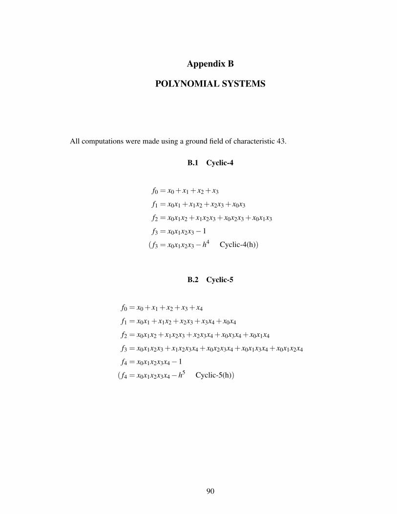
Appendix B
POLYNOMIAL SYSTEMS
All computations were made using a ground field of characteristic 43.
B.1 Cyclic-4
f0 = x0 + x1 + x2 + x3
f1 = x0x1 + x1x2 + x2x3 + x0x3
f2 = x0x1x2 + x1x2x3 + x0x2x3 + x0x1x3
f3 = x0x1x2x3−1
( f3 = x0x1x2x3−h4 Cyclic-4(h))
B.2 Cyclic-5
f0 = x0 + x1 + x2 + x3 + x4
f1 = x0x1 + x1x2 + x2x3 + x3x4 + x0x4
f2 = x0x1x2 + x1x2x3 + x2x3x4 + x0x3x4 + x0x1x4
f3 = x0x1x2x3 + x1x2x3x4 + x0x2x3x4 + x0x1x3x4 + x0x1x2x4
f4 = x0x1x2x3x4−1
( f4 = x0x1x2x3x4−h5 Cyclic-5(h))
90
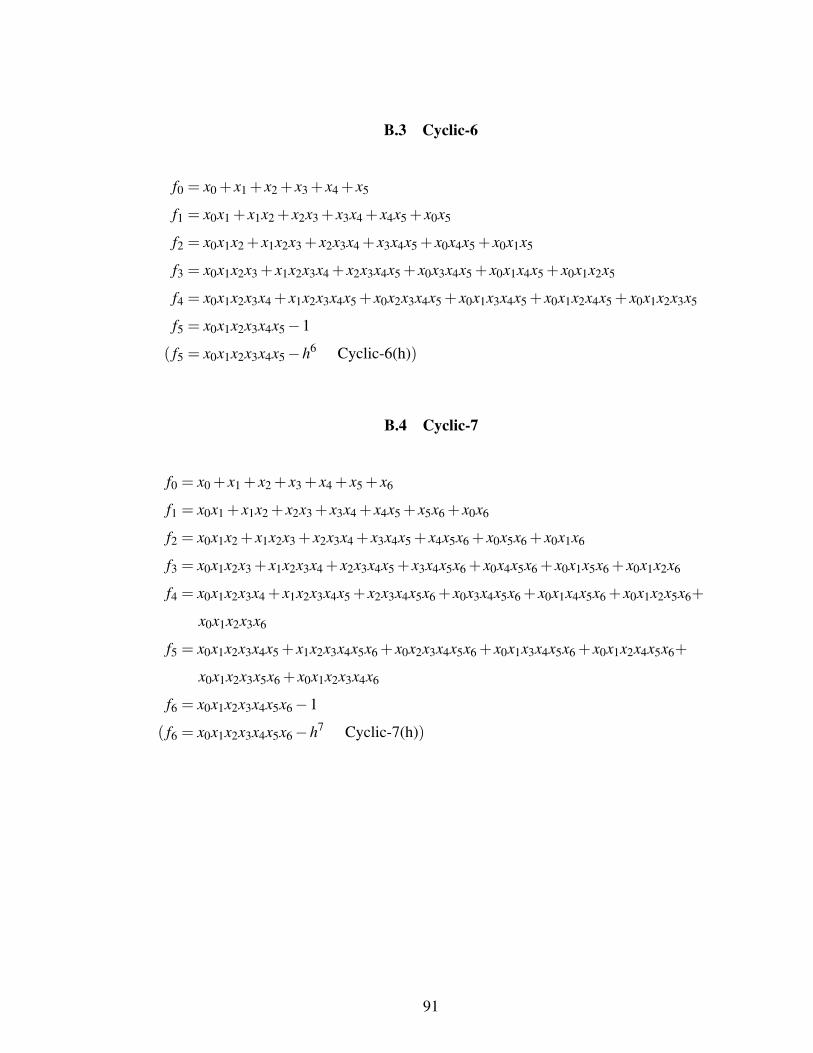
B.3 Cyclic-6
f0 = x0 + x1 + x2 + x3 + x4 + x5
f1 = x0x1 + x1x2 + x2x3 + x3x4 + x4x5 + x0x5
f2 = x0x1x2 + x1x2x3 + x2x3x4 + x3x4x5 + x0x4x5 + x0x1x5
f3 = x0x1x2x3 + x1x2x3x4 + x2x3x4x5 + x0x3x4x5 + x0x1x4x5 + x0x1x2x5
f4 = x0x1x2x3x4 + x1x2x3x4x5 + x0x2x3x4x5 + x0x1x3x4x5 + x0x1x2x4x5 + x0x1x2x3x5
f5 = x0x1x2x3x4x5−1
( f5 = x0x1x2x3x4x5−h6 Cyclic-6(h))
B.4 Cyclic-7
f0 = x0 + x1 + x2 + x3 + x4 + x5 + x6
f1 = x0x1 + x1x2 + x2x3 + x3x4 + x4x5 + x5x6 + x0x6
f2 = x0x1x2 + x1x2x3 + x2x3x4 + x3x4x5 + x4x5x6 + x0x5x6 + x0x1x6
f3 = x0x1x2x3 + x1x2x3x4 + x2x3x4x5 + x3x4x5x6 + x0x4x5x6 + x0x1x5x6 + x0x1x2x6
f4 = x0x1x2x3x4 + x1x2x3x4x5 + x2x3x4x5x6 + x0x3x4x5x6 + x0x1x4x5x6 + x0x1x2x5x6+
x0x1x2x3x6
f5 = x0x1x2x3x4x5 + x1x2x3x4x5x6 + x0x2x3x4x5x6 + x0x1x3x4x5x6 + x0x1x2x4x5x6+
x0x1x2x3x5x6 + x0x1x2x3x4x6
f6 = x0x1x2x3x4x5x6−1
( f6 = x0x1x2x3x4x5x6−h7 Cyclic-7(h))
91
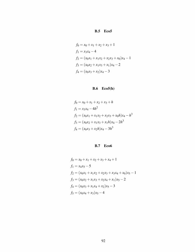
B.5 Eco5
f0 = x0 + x1 + x2 + x3 +1
f1 = x3x4−4
f2 = (x0x1 + x1x2 + x2x3 + x0)x4−1
f3 = (x0x2 + x1x3 + x1)x4−2
f4 = (x0x3 + x2)x4−3
B.6 Eco5(h)
f0 = x0 + x1 + x2 + x3 +h
f1 = x3x4−4h2
f2 = (x0x1 + x1x2 + x2x3 + x0h)x4−h3
f3 = (x0x2 + x1x3 + x1h)x4−2h3
f4 = (x0x3 + x2h)x4−3h3
B.7 Eco6
f0 = x0 + x1 + x2 + x3 + x4 +1
f1 = x4x5−5
f2 = (x0x1 + x1x2 + x2x3 + x3x4 + x0)x5−1
f3 = (x0x2 + x1x3 + x2x4 + x1)x5−2
f4 = (x0x3 + x1x4 + x2)x5−3
f5 = (x0x4 + x3)x5−4
92
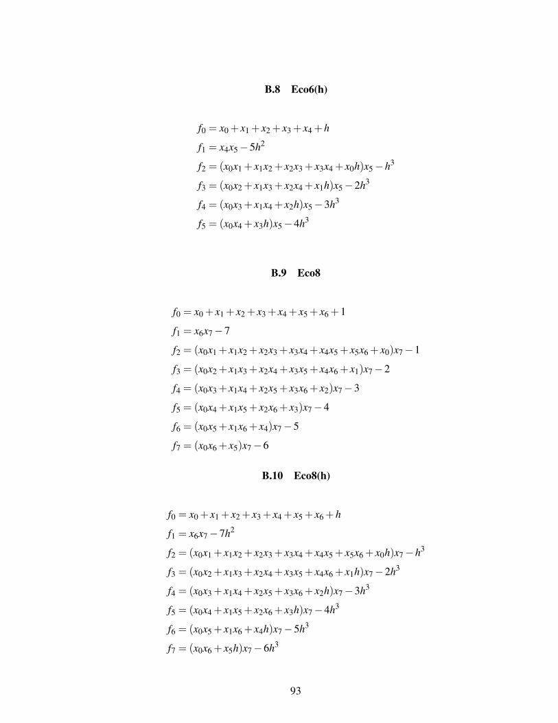
B.8 Eco6(h)
f0 = x0 + x1 + x2 + x3 + x4 +h
f1 = x4x5−5h2
f2 = (x0x1 + x1x2 + x2x3 + x3x4 + x0h)x5−h3
f3 = (x0x2 + x1x3 + x2x4 + x1h)x5−2h3
f4 = (x0x3 + x1x4 + x2h)x5−3h3
f5 = (x0x4 + x3h)x5−4h3
B.9 Eco8
f0 = x0 + x1 + x2 + x3 + x4 + x5 + x6 +1
f1 = x6x7−7
f2 = (x0x1 + x1x2 + x2x3 + x3x4 + x4x5 + x5x6 + x0)x7−1
f3 = (x0x2 + x1x3 + x2x4 + x3x5 + x4x6 + x1)x7−2
f4 = (x0x3 + x1x4 + x2x5 + x3x6 + x2)x7−3
f5 = (x0x4 + x1x5 + x2x6 + x3)x7−4
f6 = (x0x5 + x1x6 + x4)x7−5
f7 = (x0x6 + x5)x7−6
B.10 Eco8(h)
f0 = x0 + x1 + x2 + x3 + x4 + x5 + x6 +h
f1 = x6x7−7h2
f2 = (x0x1 + x1x2 + x2x3 + x3x4 + x4x5 + x5x6 + x0h)x7−h3
f3 = (x0x2 + x1x3 + x2x4 + x3x5 + x4x6 + x1h)x7−2h3
f4 = (x0x3 + x1x4 + x2x5 + x3x6 + x2h)x7−3h3
f5 = (x0x4 + x1x5 + x2x6 + x3h)x7−4h3
f6 = (x0x5 + x1x6 + x4h)x7−5h3
f7 = (x0x6 + x5h)x7−6h3
93
B.11 Katsura-5
f0 = 2x+2y+2z+2t +2u+ v−1
f1 = t2 +2xv+2yv+2zv− y
f2 = 2xt +2yu+2tu+2zv− z
f3 = 2xz+2yt +2zu+u2 +2tv− t
f4 = xy+ yz+2zt +2tu+2uv−u
f5 = 2x2 +2y2 +2z2 +2t2 +2u2 + v2− v
B.12 Noon3
f0 = 10x0x21 +10x0x2
2−11x0 +10
f1 = 10x1x20 +10x1x2
2−11x1 +10
f2 = 10x2x20 +10x2x2
1−11x2 +10
B.13 Noon4
f0 = 10x0x21 +10x0x2
2 +10x0x23−11x0 +10
f1 = 10x1x20 +10x1x2
2 +10x1x23−11x1 +10
f2 = 10x2x20 +10x2x2
1 +10x2x23−11x2 +10
f3 = 10x3x20 +10x3x2
1 +10x3x22−11x3 +10
B.14 Noon4(h)
f0 = 10x0x21 +10x0x2
2 +10x0x23−11x0h2 +10h3
f1 = 10x1x20 +10x1x2
2 +10x1x23−11x1h2 +10h3
f2 = 10x2x20 +10x2x2
1 +10x2x23−11x2h2 +10h3
f3 = 10x3x20 +10x3x2
1 +10x3x22−11x3h2 +10h3
94
B.15 Noon5
f0 = 10x0x21 +10x0x2
2 +10x0x23 +10x0x2
4−11x0 +10
f1 = 10x1x20 +10x1x2
2 +10x1x23 +10x1x2
4−11x1 +10
f2 = 10x2x20 +10x2x2
1 +10x2x23 +10x2x2
4−11x2 +10
f3 = 10x3x20 +10x3x2
1 +10x3x22 +10x3x2
4−11x3 +10
f4 = 10x4x20 +10x4x2
1 +10x4x22 +10x4x2
3−11x4 +10
B.16 Trinks
f0 = 45y+35u−165v−36
f1 = 35y+25z+40t−27u
f2 = 25yu−165v2 +15x−18z+30t
f3 = 15yz+20tu−9x
f4 =−11v3 + xy+2zt
f5 =−11uv+3v2 +99x
95
BIBLIOGRAPHY
[1] Alberto Arri and John Perry. The F5 criterion revised. Journal of Symbolic Computation,46(9):1017 – 1029, 2011.
[2] B. Buchberger. An Algorithm for Finding the Basis Elements in the Residue Class Ring Moduloa Zero Dimensional Polynomial Ideal. PhD thesis, 3 2006.
[3] Massimo Caboara. A dynamic algorithm for Gröbner basis computation. In Proceedings of the1993 International Symposium on Symbolic and Algebraic Computation, ISSAC ’93, pages275–283, New York, NY, USA, 1993. ACM.
[4] Massimo Caboara and John Perry. Reducing the size and number of linear programs in adynamic Gröbner basis algorithm. Applicable Algebra in Engineering, Communication andComputing, 25(1):99–117, Apr 2014.
[5] David A. Cox, John Little, and Donal O’Shea. Ideals, Varieties, and Algorithms: An Introduc-tion to Computational Algebraic Geometry and Commutative Algebra. Springer PublishingCompany, Incorporated, 4th edition, 2015.
[6] Christian Eder and John Perry. F5C: A variant of Faugère’s F5 algorithm with reduced Gröbnerbases. Journal of Symbolic Computation, 45(12):1442 – 1458, 2010. MEGA’2009.
[7] Christian Eder and John Edward Perry. Signature-based algorithms to compute Gröbner bases.Proceedings of the 36th International Symposium on Symbolic and Algebraic Computation -ISSAC ’11, 2011.
[8] Jean Charles Faugère. A new efficient algorithm for computing Gröbner bases without reductionto zero (F5). In Proceedings of the 2002 International Symposium on Symbolic and AlgebraicComputation, ISSAC ’02, page 75–83, New York, NY, USA, 2002. Association for ComputingMachinery.
[9] Jean-Charles Faugére. A new efficient algorithm for computing Gröbner bases (F4). Journal ofPure and Applied Algebra, 139(1):61 – 88, 1999.
[10] Alessandro Giovini, Teo Mora, Gianfranco Niesi, Lorenzo Robbiano, and Carlo Traverso. "OneSugar Cube, Please" or selection strategies in the Buchberger algorithm. In Proceedings of theISSAC’91, ACM Press, pages 5–4, 1991.
[11] Oleg Golubitsky. Converging term order sequences and the dynamic Buchberger algorithm.2007. Unpublished preprint.
[12] Peter Gritzmann and Bernd Sturmfels. Minkowski Addition of Polytopes: ComputationalComplexity and Applications to Gröbner Bases. SIAM J. Disc. Math, 6(2):246–269, 1993.
[13] Martin Kreuzer and Lorenzo Robbiano. Computational Commutative Algebra 2. Springer-Verlag Berlin Heidelberg, Berlin, Heidelberg, 2005.
96
[14] Martin Kreuzer and Lorenzo Robbiano. Computational Commutative Algebra 1. Springer-Verlag Berlin Heidelberg, Berlin, Heidelberg, 2008.
[15] G. Langeloh. Unrestricted dynamic Gröbner basis algorithms. Master’s thesis, Universi-dade Federal do Rio Grande do Sul Instituto de Informática Programa de Pós-Graduação emComputação, 3 2019.
[16] D. Lazard. Gröbner bases, Gaussian elimination and resolution of systems of algebraicequations. In J. A. van Hulzen, editor, Computer Algebra, pages 146–156, Berlin, Heidelberg,1983. Springer Berlin Heidelberg.
[17] Teo Mora and Lorenzo Robbiano. The gröbner fan of an ideal. Journal of Symbolic Computation,6(2):183 – 208, 1988.
[18] John Perry. A dynamic F4 algorithm to compute Gröbner bases. Preprint received throughprivate communication; software available at github.com/johnperry-math/DynGB.git.
[19] John Perry. Exploring the dynamic Buchberger algorithm. In Proceedings of the 2017 ACM onInternational Symposium on Symbolic and Algebraic Computation, ISSAC ’17, pages 365–372,New York, NY, USA, 2017. ACM.
[20] J.H. Silverman. A Friendly Introduction to Number Theory. Pearson Prentice Hall, 2012.
[21] The Sage Developers. SageMath, the Sage Mathematics Software System (Version 8.9), 2020.https://www.sagemath.org.
[22] Jan Verschelde. The database of polynomial systems, 2020.http://homepages.math.uic.edu/ jan/demo.html.
97