a dynamic model of sustainment investment · the model reduces the forces on sustainment investment...

A Dynamic Model of Sustainment Investment

Sarah Sheard Robert Ferguson Andrew P. Moore Mike Phillips

February 2015

TECHNICAL REPORT CMU/SEI-2015-TR-003

Software Solutions Division

http://www.sei.cmu.edu

http://www.sei.cmu.edu

Copyright 2015 Carnegie Mellon University

This material is based upon work funded and supported by the Department of Defense under Contract

No. FA8721-05-C-0003 with Carnegie Mellon University for the operation of the Software Engineer-

ing Institute, a federally funded research and development center.

Any opinions, findings and conclusions or recommendations expressed in this material are those of the

author(s) and do not necessarily reflect the views of the United States Department of Defense.

This report was prepared for the

SEI Administrative Agent

AFLCMC/PZM

20 Schilling Circle, Bldg 1305, 3rd floor

Hanscom AFB, MA 01731-2125

NO WARRANTY. THIS CARNEGIE MELLON UNIVERSITY AND SOFTWARE ENGINEERING

INSTITUTE MATERIAL IS FURNISHED ON AN “AS-IS” BASIS. CARNEGIE MELLON

UNIVERSITY MAKES NO WARRANTIES OF ANY KIND, EITHER EXPRESSED OR IMPLIED,

AS TO ANY MATTER INCLUDING, BUT NOT LIMITED TO, WARRANTY OF FITNESS FOR

PURPOSE OR MERCHANTABILITY, EXCLUSIVITY, OR RESULTS OBTAINED FROM USE

OF THE MATERIAL. CARNEGIE MELLON UNIVERSITY DOES NOT MAKE ANY

WARRANTY OF ANY KIND WITH RESPECT TO FREEDOM FROM PATENT, TRADEMARK,

OR COPYRIGHT INFRINGEMENT.

This material has been approved for public release and unlimited distribution except as restricted be-

low.

Internal use:* Permission to reproduce this material and to prepare derivative works from this material

for internal use is granted, provided the copyright and “No Warranty” statements are included with all

reproductions and derivative works.

External use:* This material may be reproduced in its entirety, without modification, and freely distrib-

uted in written or electronic form without requesting formal permission. Permission is required for any

other external and/or commercial use. Requests for permission should be directed to the Software En-

gineering Institute at [email protected].

* These restrictions do not apply to U.S. government entities.

DM-0001813

mailto:[email protected]

CMU/SEI-2015-TR-003 | i

Table of Contents

Acknowledgments iv

Executive Summary v

Abstract vii

1 Introduction 1 1.1 Why Does Sustainment Investment Need a Model? 1 1.2 Purpose of Report 2 1.3 Research Questions 2 1.4 Report Overview 2

2 Methodology 3 2.1 Modeled Sustainment Dynamics 3 2.2 Tipping Point 3 2.3 Model Evolution 4

2.3.1 Tuned Model to Partner Priorities 4 2.3.2 Defining Key Terms 6 2.3.3 Clarification of Variables 6

2.4 Model Calibration 7 2.5 Catastrophe Theory Approach Eliminated 7 2.6 Additional Stakeholders 7 2.7 SEI Publications to Date 8

3 The Systems Dynamics Model 9 3.1 Reading System Dynamics Diagrams 9 3.2 Model Overview 10 3.3 Sustainment Work 12 3.4 “Bandwagon” Reinforcing Loop (red arrows) 12 3.5 “Limits to Growth” Balancing Loop (blue arrows) 14 3.6 “Work Bigger” Balancing Loop (purple arrows) 14 3.7 “Work Smarter” Balancing Loop (dark green arrows) 15 3.8 Funding and Productivity Calculations 16

4 Scenarios 18 4.1 Equilibrium 18 4.2 Underfunding Sustainment Investment Scenario 20 4.3 Sequestration Scenario 21 4.4 New Threat, No Budget Scenario 23 4.5 Gating the Demand Scenario 26

5 Discussion 30 5.1 Tempo 30 5.2 Stakeholders and Gaps 32 5.3 Effects of Delays 35 5.4 Portfolio Considerations 35 5.5 An Additional Example of Use 36 5.6 Advice for Sustainment Organizations 37 5.7 Implications of Model Results for Sustainment Organizations 38

6 Future Work 40

CMU/SEI-2015-TR-003 | ii

6.1 Additional Modeling 40 6.2 Tuning Model 40 6.3 Continue Calibrating 40 6.4 Model Maturation 40 6.5 Model Consolidation 40

7 Conclusion 42

Appendix A Challenges to Model Validity 43

Appendix B Model Assumptions 44

Appendix C Model Variables 46

Appendix D Relationship to Army’s Sustainment WBS 49

References 51

CMU/SEI-2015-TR-003 | iii

List of Figures

Figure 1: Senge's Growth and Underinvestment Archetype 3

Figure 2: Our Initial Model, Based on Senge’s Fifth Discipline 4

Figure 3: Original Simulation Model 5

Figure 4: Example 1 – Stocks and Flows 9

Figure 5: Example 2 – Stocks and Flows with Additional Variables 10

Figure 6: Sustainment System Dynamics Model 11

Figure 7: Core Structure of Sustainment Work 12

Figure 8: Bandwagon Effect Loop 13

Figure 9: Limits to Growth Loop 14

Figure 10: Work Bigger Loop 15

Figure 11: Work Smarter Loop 16

Figure 12: Cost and Productivity Calculations 17

Figure 13: Equilibrium Mission Performance 19

Figure 14: Results of Performance for Underfunding Sustainment Investment Scenario 20

Figure 15: Results of Mission Performance Assessment for Sequestration Scenario 22

Figure 16: Results of Mission Performance Assessment for New Threat, No Budget Scenario 23

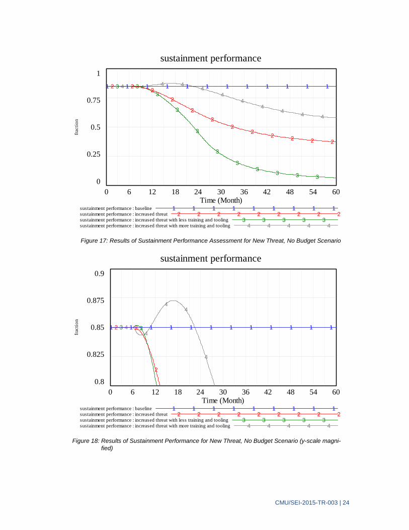
Figure 17: Results of Sustainment Performance Assessment for New Threat, No Budget Scenario 24

Figure 18: Results of Sustainment Performance for New Threat, No Budget Scenario (y-scale magnified) 24

Figure 19: Results of Mission Performance Assessment for New Threat, No Budget Scenario 25

Figure 20: Results of Mission Performance Assessment for Gating-the-Demand Scenario 27

Figure 21: Results of Mission Performance for Gating-the-Demand Scenario 28

Figure 22. Gating the Demand by Allocating Budget of Changes to Customer 29

Figure 23. Effect of Sustainment Infrastructure Funding Delays on Sustainment and Mission Performance 30

Figure 24: Cost Over Time for Sustainment 31

Figure 25: Four Types of Software Maintenance 32

Figure 26: Stakeholders and Gaps 33

Figure 27: Portfolio View 36

Figure 28: Army WBS Categories 49

Figure 29: Army WBS Category Descriptions 50

CMU/SEI-2015-TR-003 | iv

Acknowledgments

The SEI research on sustainment investment and this paper could not have been completed with-out the support of the leaders and staff of the Naval Air Warfare Center, Weapons Division at China Lake, CA. In particular, we must recognize the active participation of Jeff Schwalb, NAVAIR Associate Fellow, and the strong support of Harlan Kooima, F/A-18 and EA-18G Ad-vanced Weapons Lab IPT lead. Obtaining reliable data from a working organization requires a significant commitment by both leadership and the workforce. The effort requires a number of conversations about activity sequencing and about how to make observations of cost and time for measurement purposes. Often the researchers’ model has to change to better match the real world. Several staff members at China Lake were actively involved in reviewing the model and calibrat-ing it with data from their organization.

Additionally, we have had support and encouragement from a number of others, including Law-rence Osiecki, Director, ARDEC Armament SEC, Picatinny Arsenal, who offered suggestions for changes that improved the capability of the simulation.

CMU/SEI-2015-TR-003 | v

Executive Summary

The word “sustainment” has a broad meaning in the Department of Defense (DoD). A sustain-ment task may mean repainting a vehicle or replacing worn parts from a depot. Hardware sustain-ment such as this might then lead to a design change if a part is no longer available or if the per-formance of a component needs to be improved. The sustainment of software intensive products further changes the balance of maintenance work: Simple replacements become rare, while design changes become commonplace. This shift from maintenance to engineering means the rules for effective allocation of sustainment funds are changing, driving the need for better ways to assess the effect of decisions about those funds.

This paper describes a dynamic sustainment model that shows how budgeting, allocation of re-sources, mission performance, and strategic planning are interrelated. Since each of these pro-cesses is owned by a different stakeholder, studying the interactions over time is important. A de-cision made by one stakeholder might affect performance in a different organization. Delaying a decision to fund some work might even result in much longer delays and much greater costs to several other organizations. The model makes it possible for a decision maker (e.g., the director of a sustainment organization) to study different decision scenarios and interpret the likely effects on other stakeholders in acquisition. In this manner, DoD decision makers can mitigate problems caused by funding delays and reprioritize enhancement requests.

The model reduces the forces on sustainment investment to a set of three different performance gaps:

1. mission performance

2. sustainment performance

3. sustainment funding

Running the dynamic model with different scenarios shows the effects of interaction and delays. For example, the scenario “Gating the Demand” shows how sustainment performance increases if the sustainers take on no more work than they are able to execute. Failure to limit the requests for enhancement properly has negative consequences for mission performance.

The model was calibrated using data from the F/A-18 and EA-18G Advanced Weapons Lab (AWL) at China Lake, CA. This first attempt at calibration suggests that it would not be difficult to calibrate program data for other sustainment organizations.

CMU/SEI-2015-TR-003 | vi

CMU/SEI-2015-TR-003 | vii

Abstract

This paper describes a dynamic sustainment model that shows how budgeting, allocation of re-sources, mission performance, and strategic planning are interrelated and how they affect each other over time. Each of these processes is owned by a different stakeholder, so a decision made by one stakeholder might affect performance in a different organization. Worse, delaying a deci-sion to fund some work might result in much longer delays and much greater costs to several of the organizations.

The SEI developed and calibrated a systems dynamic model that shows interactions of various stakeholders over time and the results of four realistic scenarios. The current model has been cali-brated with data from the F/A-18 and EA-18G Advanced Weapons Lab (AWL) at China Lake, CA.

The model makes it possible for a decision maker to study different decision scenarios and inter-pret the likely effects on other stakeholders in acquisition. In a scenario where sustainment infra-structure investment is shortchanged over a period of time, the tipping point phenomenon is shown in the results of the calibrated model.

CMU/SEI-2015-TR-003 | 1

1 Introduction

1.1 Why Does Sustainment Investment Need a Model?

Sustaining weapons systems and information systems is an increasing cost concern for the Depart-ment of Defense (DoD) and the U.S. Congress [Carter 2009]. The notion of developing the neces-sary infrastructure to support new systems is already addressed in documents by Ashton Carter, For-mer Deputy Secretary of Defense, and others. However, the need to improve the sustainment infrastructure and process does not end with the initial transition to support. DoD systems tend to have a very long lifespan, often over a period of several decades. Meanwhile the development of new technologies continues and systems are constantly upgraded. Existing law is involved as well, requiring that a minimum of 50% of sustainment efforts be performed by organic support organiza-tions (service-related civilian and military personnel) rather than by external contract, but this law does not provide for the needed infrastructure improvements when workload and complexity grows.

The law is clearly designed to reduce the high overhead costs associated with creating and manag-ing contracts. Other regulations attempt to separate development costs from the costs of opera-tions and maintenance. While well intentioned, these regulations create conflicting viewpoints as to what work really constitutes enhancement versus sustainment and whether the organic sustain-ment organization or a contractor should perform the work. The pull of multiple stakeholders and complex regulations creates a system that makes decisions about funding very complicated and time consuming. The concomitant delays place a significant burden on sustainers who need funds to improve sustainment capability and capacity to meet mission demands. While this is a well-un-derstood need in the logistics community, sustainment infrastructure needs for software intensive systems are not so well understood and do not have the benefit of supporting policy.

The goal of the SEI Sustainment Investment Model is to make clear the various goals of compet-ing stakeholders and the cost of delayed decisions. The simulation model conceived here provides a mechanism for testing funding decisions to forecast effects on both sustainers and mission per-formance. The necessity to provide such forecasting tools for decision analysis has been docu-mented in several places. In The Logic of Failure: Recognizing and Avoiding Error in Complex Situations, Dietrich Dörner ran a set of simulation experiments with senior executives who had to manage resources for a country [Dörner 1996]. Resources included healthcare, water, and educa-tion. At least 90% of the executives failed to make forecasts of the effects of their decisions across all three dimensions. Failure to test the decisions over time caused widespread famine, poverty, and death. It is fortunate that the study was only a simulation.

There are two benefits to simulations: First we learn how to observe the behavior of the real sys-tem in response to our actions, and second we can test our actions in the simulation environment to see if the system responds to events and management controls by remaining within the desired bounds. While the answers from the simulation may not be terribly precise, the trends are often correct, and the simulation provides guidance about the early trends and where to look for the first evidence of potential problems.

The SEI’s simulation can help decision makers forecast the effects of funding problems and help sustainers explain why additional funds may be needed for critical infrastructure and training.

CMU/SEI-2015-TR-003 | 2

1.2 Purpose of Report

This report describes the results of a two year research study at the Carnegie Mellon Software En-gineering Institute (SEI) on the dynamics of investing in software sustainment. We created a model that describes the dynamic interactions among different stakeholders (including operational command, operational needs analysts, participants in the Program Objective Memorandum [POM] process, and the sustainment organization) and among different variables (such as the ca-pabilities of sustainment staff compared to new technology and the fraction of staff undergoing training at any given time). We validated the model via interactions with two sustainment organi-zations and calibrated it with one.

1.3 Research Questions

Two Air Force studies on sustainment postulated that sustainment organizations are or will soon be swamped by sustainment costs [USAF 2011, Eckbreth 2011]. Indeed, sustainment organiza-tions are sometimes unable to invest in needed infrastructure improvements to keep a major weapon system current unless the improvement is directly tied to a major modernization contract. Our initial observation that led to the research was one such situation where a DoD organic sus-tainment organization (with government civilian and service personnel) was denied funding for a test cell, so testing the system required cannibalizing operational equipment. Since this practice directly reduced the operational fleet “mission capable rates,” the resulting situation could easily lead to a “tipping point” where deferred modernization of the infrastructure could become so costly that the weapon system itself would be targeted for replacement [DoD 1997]. This is dis-cussed more in Section 2.1.

This research asked two questions to address this problem:

1. Can such a tipping point be modeled using the system dynamics formalism?1

2. Can the model be calibrated using data from an organization that sustains military software?

1.4 Report Overview

The contents of this report are as follows. Section 2 describes the methodology, including the cre-ation of the model, subsequent validation, and calibration. Section 3 presents the sustainment dy-namics model, the core structure for how the sustainment work is generated and processed, four types of relationship loops that explain different dynamics of the sustainment phase, and funding and productivity calculations. Section 4 provides four scenarios for exercising sustainment perfor-mance in the model. Section 5 discusses other concepts and questions that we studied during our two years of research. The report ends with a description of future work that we would like to do to continue improving the sustainment dynamics model. In the appendices, we consider chal-lenges to and assumptions in the model, define the variables we used in the model, and describe the model’s relationship to the U.S. Army’s work breakdown structure for software sustainment activities.

1 Refer to the System Dynamics Society for more information: www.systemdynamics.org.

http://www.systemdynamics.org

CMU/SEI-2015-TR-003 | 3

2 Methodology

2.1 Modeled Sustainment Dynamics

The SEI had experience with a military client who had underfunded sustainment infrastructure; as a result, the client’s software testing equipment was so old that the only way to obtain spare parts was by buying used parts on eBay. Further, the client was supporting a new radar, but no radar test kit was funded. Since this radar involved large amounts of software, the SEI was asked to help prepare a justification for funding the test kit. We considered the potential for a tipping point, at which the cost of recovery to restore software sustainment capability might be greater than the demand for the system. We then identified two potential models of this tipping point: a system dy-namics model representing the interaction of many different behaviors influencing sustainment decisions and a catastrophe theory model that showed forces as operating across a nonlinear sur-face. An investigation into the economics of the tipping-point phenomenon was proposed and then funded beginning in October 2012.

2.2 Tipping Point

Originally we modeled the tipping point on the “growth and underinvestment” archetype from Pe-ter Senge’s Fifth Discipline [Senge 1990, p. 389]. Senge’s original example has become a stand-ard MBA business case study showing the rapid growth and sudden failure of People’s Express Airlines.2 Figure 1 shows this archetype, taken from Senge’s book.

Figure 1: Senge's Growth and Underinvestment Archetype

Our initial model based on this archetype and using a systems integration lab to represent the sus-tainers appears in Figure 2. It consists of three loops:

1. reinforcing loop (with two “+”) for customer Mission Planning (top left)

2. balancing loop (one “-”) showing Operations requests for improvement (middle)

2 A description of the business case is at www.strategydynamics.com/microworlds/people-expresss/description.aspx

http://www.strategydynamics.com/microworlds/people-expresss/description.aspx

CMU/SEI-2015-TR-003 | 4

3. balancing loop showing the investment in Sustaining supporting the development of additional capability and capacity

When the effect of the balancing loops becomes too great, the need for the mission can diminish rapidly.

Mission Planning

CapabilityPlanning

SIL Delivery

SIL Capacity

Investment in SIL

Operations

+

Sustaining

_

++

_+

System Readiness

+

Perceived SIL Gaps

MissionPerformance

Changes to operational environment

+

Figure 2: Our Initial Model, Based on Senge’s Fifth Discipline

2.3 Model Evolution

The system archetype representation is too simple to represent an actual organization and must be turned into a dynamic simulation. While there are multiple forms for such simulations, we deter-mined that a “stock and flow” model should suffice. Stocks are comparable to the variables in a causal loop diagram, such as the one shown in Figure 2, and the flows are comparable to the ar-rows among them. The need to balance a few potential factors for reliable information and the po-tential for attempting to represent every possible factor is always a problem for a simulation. Many concepts of organization and workflow must be combined to create simple concepts of work queues, management controls, and work completed. If two variables are similar and have the same effect on the dynamics, they should be combined. Several iterations were needed to fine tune the balance between detail and understandability in the model.

2.3.1 Tuned Model to Partner Priorities

Our first attempt at the simulation is shown in Figure 3. When we reviewed this model with our first client, they pointed out that some of the model pertained to processes over which the sustain-ment organization had no control, in particular the governmental budgeting process. This sug-gested that we needed much less detail for that portion of the model and much more detail for the portion associated with running the sustainment organization itself. The goal was for the sustain-ment organization not only to understand the output of the sustainment investment model, but also to have the ability to make decisions and effect change.

CMU/SEI-2015-TR-003 | 5

Figure 3: Original Simulation Model3

3 While this model is difficult to read, the parts that we reused in our final model are shown again in more detail later in the document.

CMU/SEI-2015-TR-003 | 6

2.3.2 Defining Key Terms

We struggled with what “sustainment capabilities” should mean, as well as what types of demand would lead to increased requests for software changes. “Sustainment capability” signifies the types of work the organization can execute. “Capacity” means how much of that work can be performed. In the model, we define “sustainment capacity” as the product of the number of sustainers multi-plied by their average skill level (sustainment capability). While hiring more sustainers is im-portant, it is also important to sustain their skills to keep their knowledge from becoming obsolete.

We considered adding a component to the definition for capital investment in terms of equipment and tools, but discovered that the system dynamics only duplicated the effects that we saw from training alone, and that made the model more complex. Thus we removed these aspects and con-sidered training to be a proxy for “training, tooling, and other capital investments.”

2.3.3 Clarification of Variables

At least two additional cycles of model revision were required. Simplification involved identify-ing and running scenarios, understanding the dynamic effects, and tweaking the model to remove unplanned or erroneous effects caused by problems with the model.

In some cases, we realized that we meant two or more different things by one variable. An early variable was average assessed performance. We eventually determined there were at least two kinds of performance in a sustainment context: (1) The performance of the systems being sus-tained, in terms of how well they performed needed missions and (2) the performance of the sus-tainment organization. These we separated because they had different inputs and different effects. A third performance variable, program performance, was also deemed necessary to account for the number of stakeholders still committed to a program, since even if a system performs missions well, if no stakeholders are committed to using the system, the program will not thrive.

Another variable that required clarification was the demand that led to increased requests for changes. We determined that demand depends heavily on technology evolution. Technology change has at least three effects on our simulation. The first is that a sustainment organization can use better technology (e.g., test hardware, software development environment, and requirements tools) to do sustainment work. The second effect is the need to continually increase the skills of the sustainers so that they can keep up with new system hardware and software and to use these new tools. In other words, increasing technology sophistication degrades the relative skills of the sustainers unless they have ongoing training to counteract this degradation. The third effect is that threats are more sophisticated, reducing mission performance unless sustainment work is done to keep up with the changing threat environment.

We model the various types of technology change as arising from the same source: When a pulse of technology change comes in from the external world, the sustainment organization must up-grade its competencies to deal with it.

The latter two kinds of technology evolution are modeled as a single variable, a stock called Technology Sophistication. This stock is being fed by a flow called changing technology, which continually increases the level of the stock. This stock level is shown as affecting both mission performance assessment at the upper left of Figure 6 and the staff capability gap on the right.

CMU/SEI-2015-TR-003 | 7

The effect of using better technology to do sustainment work has been combined with other forms of sustainment capital investment and is modelled as equivalent to the training that is provided to the staff.

2.4 Model Calibration

Calibration is performed so that sustainment organizations can use the model for predictive pur-poses. Because calibrating the model requires using measurement data from an actual system, one of our primary concerns was how to make measured observations of variables. We worked with our second client organization for most of FY2014 to understand its sustainment organization op-erations.

We identified a number of cases where modeling abstractions were not comprehensible to a real organization. An example is counting “systems” or “capabilities.” Organizations do not provide software updates to one aircraft at a time and then start working on the next aircraft; rather they create and validate the update and then roll it out to all aircraft at once. “Capabilities” were also hard to count because it was not clear how much detail would be valuable. The final decision was to count capabilities at the level of the software specification. In some cases these were real changes to the formulas. In other cases a simple clarification of the name sufficed. To address these ambiguities, we changed the details of the model in some cases and clarified the meanings of variables in other cases. The resulting model behaves well according to the following criteria:

A steady state behavior in the model corresponds to observed data.

When an input stimulus is applied, the response of the system is similar in both timing and magnitude to observations of past behavior.

Some variable, either a stock or a flow rate (to be described in Section 3), is observable for some element of each organizational construct (i.e., sustainment, program office, operational command, or strategic planning).

2.5 Catastrophe Theory Approach Eliminated

Catastrophe theory refers to a mathematical analysis that represents effects of forces at a point on a non-linear surface, showing conditions under which a discontinuity (catastrophe) can happen. In particular, the Swallowtail catastrophe model can be used to represent the forces of the three po-tential gaps – a mission performance gap, a sustainment performance gap, and a sustainment funding gap [Weisstein 2014]; however, we soon determined that calibrating a catastrophe theory model would be difficult and not likely to provide useful insight. Further, the catastrophe theory approach might be too abstract for the real decision makers. Therefore, we made no further inves-tigation of this approach.

2.6 Additional Stakeholders

In addition to our primary calibration client, two additional stakeholders asked to be kept in-formed about the model in progress. These were two Army software engineering centers with strong interest in sustainment planning and execution. Including the initial client, we have had in-terest from the Army, Navy, and Air Force.

CMU/SEI-2015-TR-003 | 8

2.7 SEI Publications to Date

In 2006, the SEI published a technical report, Sustaining Software Intensive Systems [Lapham 2006], that served as definition and context for our own work.

The current SEI team published the article “Dynamics of Software Sustainment” in the Journal of Aerospace Information Sciences [Sheard 2014]. The article is a detailed look at the system dy-namics model as explained in Section 3. In addition, some diagrams explaining the context of sus-tainment are also included that are not included here.

Crosstalk published an article by Robert Ferguson, Mike Phillips, and Sarah Sheard called “Mod-eling Software Sustainment” [Ferguson 2014]. This article described the importance to the DoD of studying software sustainment, the problem of warfighter readiness, a preliminary set of sce-narios, and inputs and outputs of the processes represented by the model.

Two presentations were given at the National Defense Industrial Association annual conference in 2013. Sarah Sheard (with co-authors Robert Ferguson, Andrew P. Moore, D. Michael Phillips, and David Zubrow) defined the concepts of sustainment capability and capacity and showed how they were used in the model [Sheard 2013]. Robert Ferguson (with co-authors Sarah Sheard and Andrew P. Moore) created the presentation “System Dynamics of Sustainment” that contained an early version of Figure 26 and explored the effect of gaps as forces that power the model [Fergu-son 2013]. The presentation also described the testing of scenarios and the use of Senge’s arche-type to organize the system dynamics model. (As Mr. Ferguson was unable to attend, this presen-tation was delivered by Dr. Sheard).

Sarah Sheard, Andrew P. Moore, and Robert Ferguson also submitted a paper and presentation to the Conference on Systems Engineering Research in March of 2014. Titled “Modeling Sustain-ment Dynamics,” the presentation showed a preliminary version of the model and output of an early simulation of a technology pulse with various training options. The presentation was well received but due to copyright issues, the paper was unable to be published.

CMU/SEI-2015-TR-003 | 9

3 The Systems Dynamics Model

3.1 Reading System Dynamics Diagrams

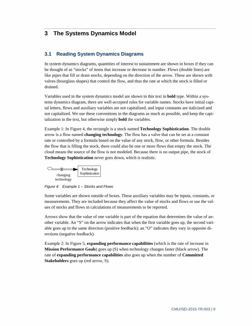
In system dynamics diagrams, quantities of interest to sustainment are shown in boxes if they can be thought of as “stocks” of items that increase or decrease in number. Flows (double lines) are like pipes that fill or drain stocks, depending on the direction of the arrow. These are shown with valves (hourglass shapes) that control the flow, and thus the rate at which the stock is filled or drained.

Variables used in the system dynamics model are shown in this text in bold type. Within a sys-tems dynamics diagram, there are well-accepted rules for variable names. Stocks have initial capi-tal letters, flows and auxiliary variables are not capitalized, and input constants are italicized and not capitalized. We use these conventions in the diagrams as much as possible, and keep the capi-talization in the text, but otherwise simply bold the variables.

Example 1: In Figure 4, the rectangle is a stock named Technology Sophistication. The double arrow is a flow named changing technology. The flow has a valve that can be set at a constant rate or controlled by a formula based on the value of any stock, flow, or other formula. Besides the flow that is filling the stock, there could also be one or more flows that empty the stock. The cloud means the source of the flow is not modeled. Because there is no output pipe, the stock of Technology Sophistication never goes down, which is realistic.

Figure 4: Example 1 – Stocks and Flows

Some variables are shown outside of boxes. These auxiliary variables may be inputs, constants, or measurements. They are included because they affect the value of stocks and flows or use the val-ues of stocks and flows in calculations of measurements to be reported.

Arrows show that the value of one variable is part of the equation that determines the value of an-other variable. An “S” on the arrow indicates that when the first variable goes up, the second vari-able goes up in the same direction (positive feedback); an “O” indicates they vary in opposite di-rections (negative feedback).

Example 2: In Figure 5, expanding performance capabilities (which is the rate of increase in Mission Performance Goals) goes up (S) when technology changes faster (black arrow). The rate of expanding performance capabilities also goes up when the number of Committed Stakeholders goes up (red arrow, S).

TechnologySophisticationChanging

Technologychanging technology

CMU/SEI-2015-TR-003 | 10

Figure 5: Example 2 – Stocks and Flows with Additional Variables

The colors of the arrows have been designed to show loops of assessment and demand. For exam-ple, the small loop of green arrows shows mission demand and assessment of performance. Each arrow in a loop has a direction of influence noted as “S” for “same” or “O” for “opposite.” We can determine whether loops are “reinforcing” or “balancing” by treating “S” as “+1” and “O” as “-1” then multiplying the +1’s and -1’s together. If the result is “+1” the loop has a reinforcing effect. When the result is “-1” the loop has a balancing effect. In a balancing loop, overall nega-tive feedback caps a rise in one of the variables. In a reinforcing loop, there is overall positive feedback so that the loop reinforces a rise in a variable (an even number of “O” effects around the loop). If an arrow is part of several loops, several arrows of different colors are shown.

3.2 Model Overview

Figure 6 shows an overview of the system dynamics model. This view shows the main loops that will be discussed below, but it does not show all the variables used in the dynamics model calcu-lation. A dataset to be used with the Vensim® commercial tool is available for readers interested in seeing all layers and all variables in the model.

To explain this model, it is necessary to break it into pieces and discuss each one. We start in the top middle with the Sustainment Work processes.

® Vensim is a registered trademark of Ventana Systems, Inc.

CMU/SEI-2015-TR-003 | 11

Figure 6: Sustainment System Dynamics Model

sustainmentcapacity

sustainmentperformance gap

BandwagonEffect

R1

Limits toGrowth

B1

S

WorkSmarter

B3

Work Bigger

B2

desired sustainmentperformance

S

TechnologySophistication

sustainmentproductivity indication

StaffAvailable

leavingstaff

hiringstaff

S

StaffCapabilityproviding

training and tools

AvailableInvestment

Funds investingfunds

allocatingfunds

yearly investmentbudget

S

ExpendedInvestment

Funds

staffcapability gap

O

S

MissionPerformance Goalsexpanding

performancegoals

CommittedStakeholdersbuying

in

PotentialStakeholders

S

S

MissionCapabilitiesImplemented

implementingcapabilities

mission capabilityrequest gap

<TechnologySophistication>

S

S

Staff InTraining

total staffS

S

startingtraining

avg cost perperson

Total StaffCostsspending on

staff

S

completingtraining

S

changingtechnology

resistance totrain or tool

O

buyingout

baselineproductivityindication

total costsO

S

RequestedStaff

requestingstaff

time to hire

O

staff count gap

S

externallyperceived

sustainmentperformance

O

resistance tohire

O

demand forupgrades

CommittedInvestment

Fundscommittingfunds

S

staffinglimit S

leaving fractionper month

S

sustainmentproductivity S

O

S

staffcapability gap

perceivedS

Ssustainmentperformance

sequestrationfraction

S

S

mission performanceassessment

S

S

S

S

S

MissionCapabilitiesScheduled

schedulingcapabilities

MissionCapabilitiesRequestedrequesting

capabilities denyingcapabilities

fractioncapabilities

denied

S

O

degradingcapabilities

fractiondegrading

S

S

performanceaveraging

period

programperformanceindication

S

S

programperformance

baseline programperformance indication

OS

leavingcapabilitiesS

TotalRequests

recordingrequests

O

O

recentMCS

S

recentMCI

S

S

O

recent TSadvances

S

S

S

S

<missionperformanceassessment>

O

S

S

time toassess

CMU/SEI-2015-TR-003 | 12

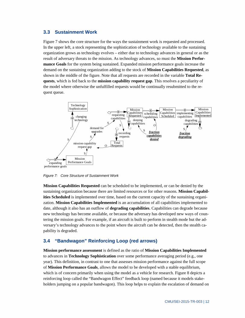
3.3 Sustainment Work

Figure 7 shows the core structure for the ways the sustainment work is requested and processed. In the upper left, a stock representing the sophistication of technology available to the sustaining organization grows as technology evolves – either due to technology advances in general or as the result of adversary threats to the mission. As technology advances, so must the Mission Perfor-mance Goals for the system being sustained. Expanded mission performance goals increase the demand on the sustaining organization adding to the stock of Mission Capabilities Requested, as shown in the middle of the figure. Note that all requests are recorded in the variable Total Re-quests, which is fed back to the mission capability request gap. This resolves a peculiarity of the model where otherwise the unfulfilled requests would be continually resubmitted to the re-quest queue.

Figure 7: Core Structure of Sustainment Work

Mission Capabilities Requested can be scheduled to be implemented, or can be denied by the sustaining organization because there are limited resources or for other reasons. Mission Capabil-ities Scheduled is implemented over time, based on the current capacity of the sustaining organi-zation. Mission Capabilities Implemented is an accumulation of all capabilities implemented to date, although it also has an outflow of degrading capabilities. Capabilities can degrade because new technology has become available, or because the adversary has developed new ways of coun-tering the mission goals. For example, if an aircraft is built to perform in stealth mode but the ad-versary’s technology advances to the point where the aircraft can be detected, then the stealth ca-pability is degraded.

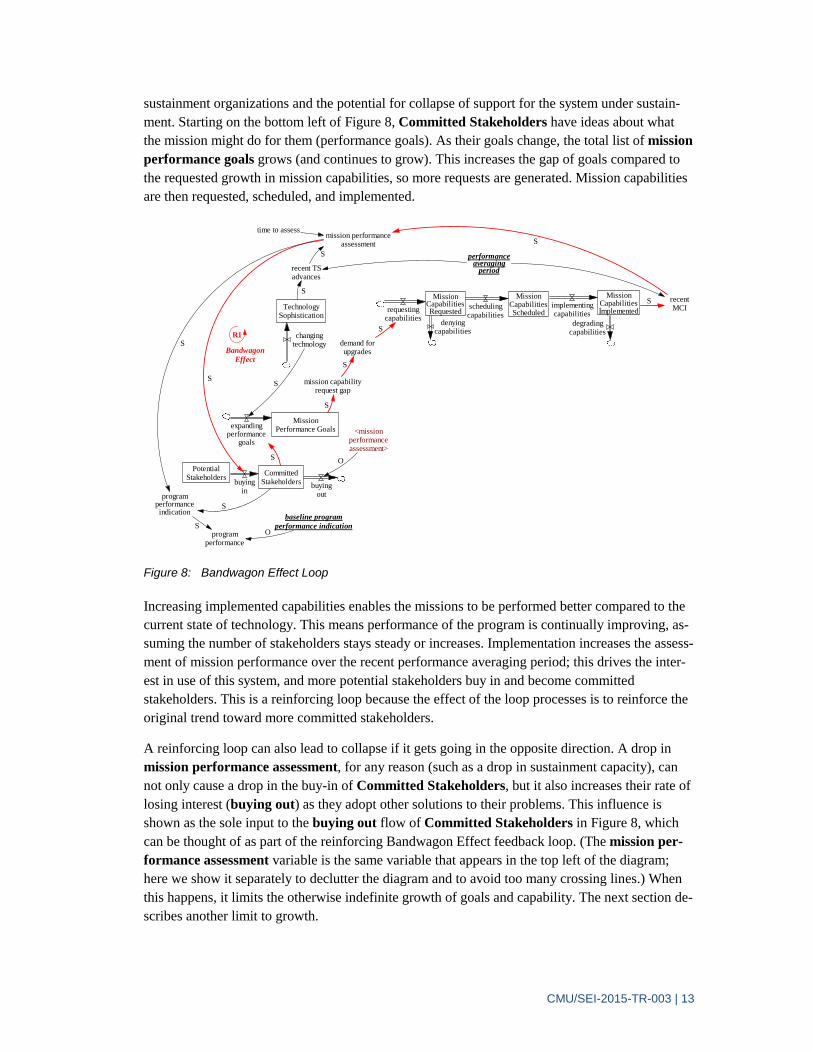
3.4 “Bandwagon” Reinforcing Loop (red arrows)

Mission performance assessment is defined as the ratio of Mission Capabilities Implemented to advances in Technology Sophistication over some performance averaging period (e.g., one year). This definition, in contrast to one that assesses mission performance against the full scope of Mission Performance Goals, allows the model to be developed with a stable equilibrium, which is of concern primarily when using the model as a vehicle for research. Figure 8 depicts a reinforcing loop called the “Bandwagon Effect” feedback loop (named because it models stake-holders jumping on a popular bandwagon). This loop helps to explain the escalation of demand on



performance goals




S

changingtechnology

demand forupgrades

S

S

S




capabilitiesdenying

capabilities

fractioncapabilities

denied

S

O


fractiondegrading

S

TotalRequests

recordingrequests

O

S

CMU/SEI-2015-TR-003 | 13

sustainment organizations and the potential for collapse of support for the system under sustain-ment. Starting on the bottom left of Figure 8, Committed Stakeholders have ideas about what the mission might do for them (performance goals). As their goals change, the total list of mission performance goals grows (and continues to grow). This increases the gap of goals compared to the requested growth in mission capabilities, so more requests are generated. Mission capabilities are then requested, scheduled, and implemented.

Figure 8: Bandwagon Effect Loop

Increasing implemented capabilities enables the missions to be performed better compared to the current state of technology. This means performance of the program is continually improving, as-suming the number of stakeholders stays steady or increases. Implementation increases the assess-ment of mission performance over the recent performance averaging period; this drives the inter-est in use of this system, and more potential stakeholders buy in and become committed stakeholders. This is a reinforcing loop because the effect of the loop processes is to reinforce the original trend toward more committed stakeholders.

A reinforcing loop can also lead to collapse if it gets going in the opposite direction. A drop in mission performance assessment, for any reason (such as a drop in sustainment capacity), can not only cause a drop in the buy-in of Committed Stakeholders, but it also increases their rate of losing interest (buying out) as they adopt other solutions to their problems. This influence is shown as the sole input to the buying out flow of Committed Stakeholders in Figure 8, which can be thought of as part of the reinforcing Bandwagon Effect feedback loop. (The mission per-formance assessment variable is the same variable that appears in the top left of the diagram; here we show it separately to declutter the diagram and to avoid too many crossing lines.) When this happens, it limits the otherwise indefinite growth of goals and capability. The next section de-scribes another limit to growth.

BandwagonEffect

R1



performancegoals


in


S




S

changingtechnology

buyingout

demand forupgrades

mission performanceassessment

S

S

S

S




capabilitiesdenying

capabilitiesdegrading

capabilities


period

programperformanceindication

S

S

programperformance

baseline programperformance indication

OS

recentMCI

S

recent TSadvances

S

S

S

<missionperformanceassessment>

O

time to assess

CMU/SEI-2015-TR-003 | 14

3.5 “Limits to Growth” Balancing Loop (blue arrows)

Sustainment Performance is shown in the middle of Figure 6. It is defined as

(Mission Capabilities Implemented) . (Mission Capabilities Implemented + Mission Capabilities Scheduled)

where all quantities are the totals over the performance averaging period. Good performance keeps this ratio high, showing that capabilities are not stacking up in the scheduled queue without being implemented.

Figure 9 depicts another influence on Committed Stakeholders’ buying out of support for the system under sustainment. If the number of Mission Capabilities Implemented (shown in the box on right in Figure 9) fails to keep pace with the number of Mission Capabilities Scheduled, then sustainment performance is low and perceived as inadequate. Therefore, Committed Stake-holders fear obsolescence or lack of availability of the system, and then decide to use some other system to perform their mission. This reduces the contribution that increasing stakeholder goals makes to the Mission Performance Goals. (The other contributor, the ongoing march of new technology, continues to increase Mission Performance Goals.) In response, the demand for up-grades and requests for sustainment capabilities is decreased, and the number of Mission Capa-bilities Scheduled to be implemented also drops. This reduces the gap between scheduled and achieved capabilities, balancing out the original drop in performance.

Figure 9: Limits to Growth Loop

3.6 “Work Bigger” Balancing Loop (purple arrows)

Figure 10 shows a sustainment performance gap, calculated as the difference between the de-sired and perceived performance of the sustainment organization. This is interpreted as a need to increase the staff count. If additional staff will not violate a staffing limit, hiring requests are cre-ated. After a delay for time to hire, staff members become available, leading to an increase in sus-tainment capacity which causes work to be done faster and reduces the performance gap (note that

Limits toGrowth

B1



performancegoals


in


S




changingtechnology

buyingout externally

perceivedsustainmentperformance

O

demand forupgrades


S




capabilities denyingcapabilities

S

S

Sdegrading

capabilities

S


period

recentMCS

S

recentMCI

S

S

O

CMU/SEI-2015-TR-003 | 15

staff can also leave, and a higher amount of sequestration—which means forced time off without pay—increases departures).

Figure 10: Work Bigger Loop

3.7 “Work Smarter” Balancing Loop (dark green arrows)

Figure 11 shows the same Staff Available as one of the two inputs into sustainment capacity. The other input is Staff Capability. Staff Capability is fundamental to the Work Smarter loop, which contrasts with the Work Bigger loop described in the previous section.

sustainmentcapacity

sustainmentperformance gap

S

Work Bigger

B2

desired sustainmentperformance

S

StaffAvailable

leavingstaff

hiringstaff

S



RequestedStaff

requestingstaff

time to hire

O

staff count gap

S

resistance tohire

O

staffinglimit S


S

S



S



O

recentMCS

S

recentMCI

S

O

S

CMU/SEI-2015-TR-003 | 16

Figure 11: Work Smarter Loop

All staff members need to complete training, and that includes newly hired staff. Training staff increases the capability of the trained staff, so capacity increases as staff completes training. Pull-ing staff away from implementing mission capabilities of the sustained systems to go to training increases the capability of the trained staff but temporarily decreases sustainment capacity. Tools are also listed since providing good tools and the education needed to use them has the same effect on staff capability as increasing training (process improvement can do the same, but this is not explicitly shown). The increase in Staff Capability is shown as decreasing the staff ca-pability gap with respect to the current Technology Sophistication, resulting in less need for training to close the gap (i.e., the self-balancing aspect of the Work Smarter feedback loop). Per-haps more important, increases in Staff Capability also increase the sustainment capacity, which improves the mission and sustainment performance of the organization.

3.8 Funding and Productivity Calculations

Calculations of sustainment cost and sustainment productivity are also available in the model, but are not shown above. Total costs is calculated (on the bottom of Figure 12) from the Total Staff Costs plus the Expended Investment Funds spent on training and tools. (The various funds stocks and flows represent usage of the budgeted funds as people start and then complete train-ing.) Total Staff Costs are the sum of available staff plus staff currently pulled out for training, multiplied by the average cost per person.

Sustainment productivity is calculated as the achieved sustainment performance divided by the sustainment cost (over a calculated performance averaging period), normalized by the baseline productivity.

sustainmentcapacity

WorkSmarter

B3

StaffAvailable

leavingstaff


training and tools

staffcapability gap

O

<TechnologySophistication>

S

Staff InTraining

startingtraining

completingtraining

S

resistance totrain or tool

O


S

S

staffcapability gap

perceived

SS


Sleaving

capabilitiesS

S

CMU/SEI-2015-TR-003 | 17

Figure 12: Cost and Productivity Calculations

sustainmentproductivity indication

StaffAvailable


training and tools

AvailableInvestment

Funds investingfunds

allocatingfunds

yearly investmentbudget

S

ExpendedInvestment

Funds

S

S

Staff InTraining

total staffS

S

startingtraining

avg cost perperson

Total StaffCostsspending on

staff

S

completingtraining

S

baselineproductivityindication

total costsO

S

CommittedInvestment

Fundscommittingfunds

S

sustainmentproductivity S

O


S

S

S

CMU/SEI-2015-TR-003 | 18

4 Scenarios

This section describes the setup of the simulation based on the model we described in Section 3. Each variable is given an initial value, ideally an input from a particular organization (such as staff count) or an amount chosen when making the model run in equilibrium mode. The table in Appendix C lists all the variables and describes how the values were determined. The simulation was run, meaning the values of key variables were tracked on a monthly basis for 60 months and graphed to show their dynamic changes over time. We also show the results of these simulation runs in this section.

Two steps are required to validate that a system dynamics model properly represents a real-world system. First we must establish a baseline in which the model remains in equilibrium. In this base-line, several critical variables in the model have values corresponding to observations of the real organizational system. At least one variable representing either a stock or flow from each section can be given a value that can be observed in the real world. Equilibrium means that the stocks and flows remain constant with those values. Next, the model is re-run using a scenario of change. For each scenario, only one or two inputs are changed. As a result, the stimulus sets the model into motion, and it is possible to observe the effects. If the model has been properly designed and cali-brated, the observations of the model should match well to observations in the real world.

The four scenarios used for testing, in addition to the baseline, are:

1. Underfunding Sustainment Investment: A new capability is provided for flight equip-ment, but no funding for sustainment upgrades or software test equipment is provided.

2. Sequestration: Facility staff members are required to take unpaid time off.

3. New Threat, No Budget: A technology threat appears that must be addressed, but no ad-ditional sustainment funding is available.

4. Effects of Gating the Demand: The sustainment organization can only provide a steady amount of capabilities upgrades due to lack of additional funding. This means that a large fraction of requested upgrades are not accepted every year.

These five situations (the equilibrium baseline plus the four scenarios) are described in the follow-ing sections. For each of the non-equilibrium scenarios, the baseline runs for a simulation time equivalent to six months, and then the change stimulus is applied. The model is allowed to run for an additional simulation time equivalent to four-and-a-half years.

4.1 Equilibrium

Simulation results are described with respect to a model equilibrium, which is shown in simula-tion graphs as a “baseline” simulation run. The equilibrium of the model described in this paper ensures that all stocks remain at a constant value (possibly zero). In equilibrium, a model is easier to experiment with since the analyst can more easily determine how small changes in input affect the overall behavior of the simulation. Any change in behavior (as seen in the behavior-over-time graphs) can be attributed to that single changed input and only that change. It is analogous in sci-entific experiments to keeping all variables constant (i.e., the independent or controlled variables)

CMU/SEI-2015-TR-003 | 19

except the ones being studied (i.e., the dependent variables). The equilibrium values of the key model variables are described in Appendix B, Model Assumptions.

Each of these scenarios is described in a box that includes the following:

operational context

external stimulus or a change in strategy such as resource allocation

response generated by the organizations being simulated

predicted observable outcome exhibited by the simulated system or the expected outcome that we wish to check by running the simulation

A graph of results is then shown (i.e., a calculated value of a variable in the model), followed by a paragraph discussing what the results mean. In a results graph, the vertical axis shows the value of mission performance assessment. Mission performance is a dimensionless variable that varies be-tween 0 (indicating mission performance does not have any value to the warfighter) and 1 (indi-cating the mission has perfect value). If equilibrium had a mission performance of 0.75, and a sce-nario now has a mission performance of 0.5, the mission performance is interpreted as only 2/3 of the baseline value. For the equilibrium case, this is set to between 0.75 and 0.85 in different runs. The value is not as important as how it changes under the scenario conditions.

The horizontal axis is time; sequestration begins at month 6 and the scenario is run for five years (60 months). As an example, Figure 13 shows just the equilibrium mission performance for the first scenario.

Figure 13: Equilibrium Mission Performance

CMU/SEI-2015-TR-003 | 20

4.2 Underfunding Sustainment Investment Scenario Underfunding occurs when the sustainers are made responsible for the support of a new technol-ogy, but there is no budgetary provision to support tooling, process changes, and staff training. The question to ask is whether this shortcoming will affect the mission readiness and how long it will take before shortcomings in mission readiness can be observed.

Context Operational capability is currently in use in theater. System capability is currently sustained by

an organic unit such as a military Software Engineering Center.

Stimulus Contractor updates hardware and software with new software-controlled radar. Program uses all its funds and cannot afford to pay for a radar kit to be used by the Organic Sustainment or-ganization to test ongoing software maintenance releases.

Response This scenario usually generates the “work bigger” response (see Sec. 3.6). The sustainers take on additional activity in order to accommodate the new technology. When the software for the radar is updated, an operational aircraft must be brought to the facility where the radar is then removed to a test stand. Once testing is satisfactorily completed, the radar must be re-installed and re-calibrated to the aircraft. An operational aircraft is out of service for the duration. The cost of testing is increased by the support required to disassemble and reassemble the radar on its platform. There is additional pressure on the test team to work fast and return the aircraft to the fleet.

Outcome Mission performance is expected to degrade at some future date since sustainers cannot oper-ate at the same efficiency and productivity as before. Testing shortcuts may allow additional de-fects to leak to the field. Sustainment throughput is slowed or costs increase because of the ex-tra work. Product satisfaction may fall off if additional defects are delivered. There is risk of breaking functional operating equipment due to excessive handling. Operational readiness of the fleet may be affected if the fleet is very small.

Results

Figure 14: Results of Performance for Underfunding Sustainment Investment Scenario

Performance Comparison

1

0.75

0.5

0.25

0

4 4 4 4 44

44

4

4

4

3 3 33

33

3

3

3

3

3

2 2 2 2 2 2 2 2 2 2 2 21 1 1 1 1 1 1 1 1 1 1 1

0 6 12 18 24 30 36 42 48 54 60Time (Month)

frac

tion

sustainment performance : baseline 1 1 1 1 1 1 1 1 1mission performance assessment : baseline 2 2 2 2 2 2 2 2 2sustainment performance : 80% investment budget cut 3 3 3 3 3 3 3mission performance assessment : 80% investment budget cut 4 4 4 4 4 4

CMU/SEI-2015-TR-003 | 21

Interpretation

This graph shows mission performance assessment as compared to the baseline that results from an 80% cut4 in the capital funding (tooling and training the sustainment) at month 6. Although for a very short time performance improves due to the effects of “work bigger” rather than training, there is a gradual but steady decline starting at about month 12. Mission performance decreases during the simulation to a performance level of 0.63 (from the 0.75 equilibrium) with no sign of slowing the productivity decline.

The mission performance decline begins at about month 18, but by month 36 it has declined by about 6%. Note that the decline in mission performance lags the decline in sustainment perfor-mance by 12-18 months. With that much delay, those responsible for mission performance may not make the connection to the decline in sustainment performance, and may attribute it to other causes. Similarly, if we then begin to improve sustainment performance, it will take time for the sustainers to achieve the desired level and another 12-18 months for mission performance to achieve its operational goal. This effect is so far removed from the change to the sustainment or-ganization that the cause may escape recognition.

Exactly how much time passes between reducing infrastructure funding and the corresponding de-crease in sustainment performance will differ according to the pace of technology change and the initial quality of the products being sustained. The time delay between sustainment perfor-mance and the effect on mission performance assessment will also be affected by the time re-quired for deployment plus the time between major mission assessment events.

4.3 Sequestration Scenario

In this scenario, the government cuts staffing to reduce budget. We want to examine how the loss of staff plus the elimination of training affects sustainment capacity and operational mission performance assessment.

Context Normal sustainment work at a weapons test facility.

Stimulus Congress decides that Federal workers should work only 4 days/week to reduce costs by 20%.

Response Facility reduces staff attendance by 20%. In order to accomplish necessary work the leader cuts out all training (thus keeping people available for immediate work).

Outcome Normal training is 40-60 hrs/year/person, or in the range of 2-4% of staff time. Effects of seques-tration will depend on duration and number of personnel affected. In the short term, effects are likely to be minimal. If sequestration lasts for 12 months and 100 people are affected, then 20 staff months is the total effect on capacity. The total effect of eliminating training is a staff equiva-lent of 2-3 full-time-equivalents. Hiring is also eliminated during sequestration, so attrition has a more significant effect as well. Attrition in engineering DoD staff is typically low, between 5-8% per annum. At 5%, the additional personnel loss is about 2 fewer staff available at the end of se-questration.

4 One sustainment organization we worked with often gets only 20-25% of its budget requests granted.

CMU/SEI-2015-TR-003 | 22

Results

Figure 15: Results of Mission Performance Assessment for Sequestration Scenario

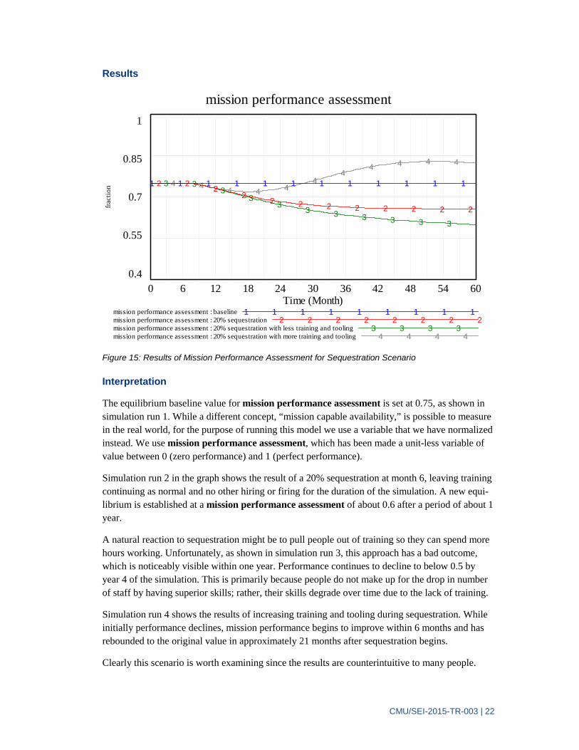
Interpretation

The equilibrium baseline value for mission performance assessment is set at 0.75, as shown in simulation run 1. While a different concept, “mission capable availability,” is possible to measure in the real world, for the purpose of running this model we use a variable that we have normalized instead. We use mission performance assessment, which has been made a unit-less variable of value between 0 (zero performance) and 1 (perfect performance).

Simulation run 2 in the graph shows the result of a 20% sequestration at month 6, leaving training continuing as normal and no other hiring or firing for the duration of the simulation. A new equi-librium is established at a mission performance assessment of about 0.6 after a period of about 1 year.

A natural reaction to sequestration might be to pull people out of training so they can spend more hours working. Unfortunately, as shown in simulation run 3, this approach has a bad outcome, which is noticeably visible within one year. Performance continues to decline to below 0.5 by year 4 of the simulation. This is primarily because people do not make up for the drop in number of staff by having superior skills; rather, their skills degrade over time due to the lack of training.

Simulation run 4 shows the results of increasing training and tooling during sequestration. While initially performance declines, mission performance begins to improve within 6 months and has rebounded to the original value in approximately 21 months after sequestration begins.

Clearly this scenario is worth examining since the results are counterintuitive to many people.

mission performance assessment

1

0.85

0.7

0.55

0.4

4 44 4 4

44

4 4 4 4

3 33

33

3 3 3 3 3 3

2 22

22 2 2 2 2 2 2 2

1 1 1 1 1 1 1 1 1 1 1 1

0 6 12 18 24 30 36 42 48 54 60Time (Month)

frac

tion

mission performance assessment : baseline 1 1 1 1 1 1 1 1 1mission performance assessment : 20% sequestration 2 2 2 2 2 2 2 2mission performance assessment : 20% sequestration with less training and tooling 3 3 3 3mission performance assessment : 20% sequestration with more training and tooling 4 4 4 4

CMU/SEI-2015-TR-003 | 23

4.4 New Threat, No Budget Scenario

In this scenario, a new threat is discovered. The system is upgraded but there may not be money for training and tooling. We want to see how long it takes for mission performance to decline and by how much.

Context Operational capability is currently in use in the theater. System capability is currently sustained by an organic unit, such as a military Software Engineering Center.

Stimulus Mission effectiveness is challenged by a new threat. The threat warrants an upgrade to the sys-tem capability. The cost of the upgrade is approximately $100M if performed by the sustainment organization and can be executed to completion within 12 months.

Response The operational command requests an upgrade. The Program Office agrees to make the up-grade a priority, but only operations and maintenance (O&M) funding and the current budget are available. This amount is insufficient to meet the need required for the enhancement; therefore the budget must come via the congressional budgeting cycle.

Outcome Additional funding is sought and provided, but it takes 12 months or more to reach the sustaining organization. Delivery of additional capability takes 12 months after funding is made available.

Results

Figure 16: Results of Mission Performance Assessment for New Threat, No Budget Scenario


0.8

0.6

0.4

0.2

0

44

4

44

4 4 4 4 4 4

3 3

3

3

3

3

3

33

33

3

2 2

2

2

2

22

22 2 2 2

1 1 1 1 1 1 1 1 1 1 1 1

0 6 12 18 24 30 36 42 48 54 60Time (Month)

frac

tion

mission performance assessment : baseline 1 1 1 1 1 1 1 1 1mission performance assessment : increased threat 2 2 2 2 2 2 2 2mission performance assessment : increased threat with less training and tooling 3 3 3 3mission performance assessment : increased threat with more training and tooling 4 4 4 4

CMU/SEI-2015-TR-003 | 24

Figure 17: Results of Sustainment Performance Assessment for New Threat, No Budget Scenario

Figure 18: Results of Sustainment Performance for New Threat, No Budget Scenario (y-scale magni-fied)

sustainment performance

1

0.75

0.5

0.25

0

4 4 4 44

44

44

4 4

3 33

3

3

3

33

3 3 3

2 22

2

2

22

22 2 2 2

1 1 1 1 1 1 1 1 1 1 1 1

0 6 12 18 24 30 36 42 48 54 60Time (Month)

frac

tion

sustainment performance : baseline 1 1 1 1 1 1 1 1 1sustainment performance : increased threat 2 2 2 2 2 2 2 2 2sustainment performance : increased threat with less training and tooling 3 3 3 3 3sustainment performance : increased threat with more training and tooling 4 4 4 4 4

sustainment performance

0.9

0.875

0.85

0.825

0.8

44

44

4

3 32 2

2

1 1 1 1 1 1 1 1 1 1 1 1

0 6 12 18 24 30 36 42 48 54 60Time (Month)

frac

tion

sustainment performance : baseline 1 1 1 1 1 1 1 1 1sustainment performance : increased threat 2 2 2 2 2 2 2 2 2sustainment performance : increased threat with less training and tooling 3 3 3 3 3sustainment performance : increased threat with more training and tooling 4 4 4 4 4

CMU/SEI-2015-TR-003 | 25

Figure 16 plots the mission performance assessment. As with previous scenarios, the mission performance declines precipitously; more training and tooling provides the best mission perfor-mance. In contrast, both Figure 17 and Figure 18 show sustainment performance, at different vertical scales. Sustainment performance is a measure of how well the sustaining organization is completing its committed work. Figure 17 shows that the sustainment organization can maintain its own performance only by increasing its training and tooling. Figure 18 has the same time pe-riod as Figure 17, but we have zoomed in on the vertical axis to highlight the immediate changes that occur between months 6 and 18. Close examination of Figure 18 shows an immediate slight performance improvement is obtained by reducing training and tooling (curve 3). However, that improvement evaporates after only two months. On the other hand, increasing tooling and training (curve 4) appears to have a deleterious effect on sustainment performance for about 6 months before performance improves and remains higher than both curve 2 (constant training) and curve 3 (reduced training). With modifications to training and tooling engaged at month 6 when the threat change occurs, one can see why organizations are rewarded in the short term for pulling people out of training and tooling to cover for the greater threat. This “better before worse” be-havior can fool the manager who has not looked forward a few additional months. This scenario shows that if managers can plan beyond the time period of reduced performance, they may choose to increase training and tooling as a means to manage for increased threat.

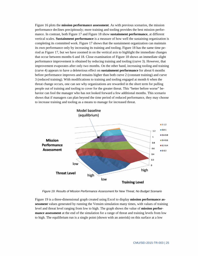
Figure 19: Results of Mission Performance Assessment for New Threat, No Budget Scenario

Figure 19 is a three-dimensional graph created using Excel to display mission performance as-sessment values generated by running the Vensim simulation many times, with values of training level and threat level ranging from low to high. The graph shows the value of mission perfor-mance assessment at the end of the simulation for a range of threat and training levels from low to high. The equilibrium run is a single point (shown with an asterisk) on this surface at a low

*

CMU/SEI-2015-TR-003 | 26

threat level and medium training level that generates the equilibrium mission performance as-sessment of 0.75. Of note in this figure is the steep decline in performance that results from low levels of training at all levels of threat.

Interpretation

This scenario is particularly interesting because it can be considered counter-intuitive. Even with no budget increase, the sustainers should allocate more funds to training and infrastructure (and thus less to work per se) in order to decrease the long-term impacts of underfunding. New threats and new technology have to be addressed by tooling and training within a few months even at the cost of delaying a release, because shorter term productivity objectives can no longer be achieved in any case.

The equilibrium baseline value for mission performance assessment is 0.75, as shown in simula-tion run 1. (The equilibrium baseline is the same for all four scenarios.) During the first 12 months all scenarios are similar.

Simulation run 2 in the graphs shows the result of a doubling of the threat at month 6, until the end of the simulation, with no other hiring or firing for the duration. A new equilibrium is estab-lished at about 0.24 or about a third of initial mission performance assessment.

Simulation run 3 shows the results of pulling people out of training, which not only does not solve the problem even in the near term, but actually causes mission performance assessment to drop to below 0.1 by the end of the five-year time horizon.

Simulation run 4 shows the results of an aggressive training and tooling campaign to increase the effectiveness of existing staff, following the increased threat. The mission performance assess-ment starts doing better than the other runs after 3 months and plateaus to above 0.4 by the end of the simulation.

Declines in operational mission performance assessment can cause the operational commanders and the program office to assume the sustainers are not capable. Thereby both the operational command and program office may be more inclined to seek funding for a new contract with a DoD supplier. The simulation suggests the possibility that the organic sustainers are typically un-derfunded and that the DoD pays twice for training the sustainment process – once for the con-tracted development organization and again for the organic sustainment organization. Further-more, creating a new contract takes many months or even years, so mission capability may be severely delayed.

4.5 Gating the Demand Scenario

In this scenario, the sustainment organization chooses to deny a number of otherwise valid re-quests for the sole reason that the organization does not have capacity to fulfil the requests. Clearly this will delay implementation of all requests that are denied. What will it do to sustain-ment performance and to mission performance assessment?

CMU/SEI-2015-TR-003 | 27

Context Normal sustainment operations have a restrictive budget and little flexibility to hire.

Stimulus Requests for product improvement are greater (number and complexity) than the sustainer is able to supply.

Response Sustainer may restrict the number of enhancement requests allowed. Is it better to over-promise and under-deliver or limit the number of requests to keep it within the capacity for the work?

Outcome We expect that sustainment performance may go up, because the same amount of work can be concentrated on a smaller number of approved requests.

Results

Software sustainment organizations have frequently reported that accepting too much work causes them to delay product releases. The simulation shows that delaying the release (releasing at a slower rate) does indeed compromise mission performance. Of course, the degradation of mission performance appears later, so the relationship is not immediately apparent.

Figure 20: Results of Mission Performance Assessment for Gating-the-Demand Scenario

Interpretation

Like the prior example of “New Threat, No Budget,” this graph shows that limiting the number of enhancement requests accepted to the limits of available productivity is good for both the sustain-ers and the mission. Gated demand allows the sustaining organization to operate with fewer re-sources or at higher levels of sustainment performance than would otherwise be possible. (In addition, it allows organizational decision makers to assign all resources to the highest priority re-quests, though priorities are not modeled explicitly in our simulations.) Thus, low levels of deny-ing mission capability requests may not have any negative impact on mission performance. How-ever, with medium levels of denial of mission capability, requests start to show deleterious effects


0.8

0.6

0.4

0.2

0

4 44

4

4

4

4

44

44

3 3 3 33

33

33

3 3 3

2 2 2 2 2 2 2 2 2 2 2 21 1 1 1 1 1 1 1 1 1 1 1

0 6 12 18 24 30 36 42 48 54 60Time (Month)

frac

tion

mission performance assessment : baseline 1 1 1 1 1 1 1 1mission performance assessment : low demand gate 2 2 2 2 2 2mission performance assessment : medium demand gate 3 3 3 3 3 3mission performance assessment : high demand gate 4 4 4 4 4 4 4

CMU/SEI-2015-TR-003 | 28

on mission performance, which drops to about 0.4 by the end of the simulation. High levels of denying mission capability requests result in mission performance levels below 0.1.

Achieving the optimal balance of approved requests using only the available funds requires so-phistication in the decision process.

Results

Figure 21: Results of Mission Performance for Gating-the-Demand Scenario

Figure 19 is a three-dimensional graph created using Excel to display program performance val-ues generated by running the Vensim simulation many times, with values of threat level ranging from low to high, and with a low to high amount of capability that is denied. The graph shows the value of program performance at the end of the simulation for a range of denied capability and threat levels. The equilibrium run is a single point (shown with an asterisk) on this surface at a low threat level and low training level that generates the equilibrium program performance level of 1.0. As described in Section 2.3.3, program performance is the mission performance assess-ment multiplied by the number of Committed Stakeholders still engaged.

Of note in this figure is the slow rise in program performance possible at low levels of gated de-mand, and the rapid drop in program performance for medium and high levels of gated demand, at all levels of threat. The rapid drop is due to stakeholders buying out of the sustainment due to the dropping performance levels (i.e., the bandwagon effect running in reverse). A likely reason for such “buying out” is an expensive modernization contract with its own overhead and time-consuming and costly contracting process.

*

CMU/SEI-2015-TR-003 | 29

Example of Gating the Demand

One of our collaborating organizations has been making effective use of “Gating the Demand” as follows:

The original source line of code (SLOC) budget for a release was set at 11,000 SLOC. Of this amount, the contractor determined that a contingency budget of 20% (~2,000 SLOC) should be set aside for code growth. Of the contingency budget, the contractor retained 75% and offered 25%, or 500 SLOC, to the customer for additional changes. That budget was to be used according to Figure 22 based on the calendar. Each new bar represents the maximum amount of change that will be accepted after the date at the bottom. Thus, the contractor is gating the change requests so to be certain of delivering on schedule.

Figure 22. Gating the Demand by Allocating Budget of Changes to Customer

As the work progressed, the contingency available for new requirements disappeared incremen-tally. The budget for new requests dropped to 200 SLOC by October and eventually to no new re-quests by December, when testing was scheduled to begin.

This contractor has been able to achieve high levels of both predictability and quality.

CMU/SEI-2015-TR-003 | 30

5 Discussion

In this section we explore the implications of our results and address some related topics that we investigated during the course of our research.

The bottom line is that if funding is not provided in a timely manner to maintain the sustainment infrastructure (tooling, training, and process improvement), then sustainment capability and ulti-mately the mission-capable performance of the fleet will be adversely impacted. Figure 23 shows that budget cuts affect both sustainment performance and mission performance assessment, with sustainment performance hurt as soon as six months after the budget cut at month 6, and mis-sion performance seriously damaged but not even starting until a year after the cut occurs. This might make it difficult for decision makers to identify the cause of mission performance degrada-tion.

Figure 23. Effect of Sustainment Infrastructure Funding Delays on Sustainment and Mission Perfor-mance

Additional topics in this section include the varying tempos of activities related to sustainment; sustainment stakeholders and the decision-making inputs that we are calling “gaps,” considera-tions related to sustainment organizations managing a portfolio of systems—not just one program; the effect of delays; an example of use of this model in a different context; and concrete advice.

5.1 Tempo

A dynamic model was essential for this work as each of the stakeholders experiences a different frequency in the work. The effects of the different frequencies appear in Figure 24.

sustainment performance and mission performance assessment

CMU/SEI-2015-TR-003 | 31

Figure 24: Cost Over Time for Sustainment

The chart is adapted from an Army study and shows a pattern of block releases for software up-dates. Each bar represents the cost of a block release of the system. Most of the block releases have a flat budget, are small and consist mostly of bug fixes. Every few releases, there are some new enhancements (red bars) and the block will cost 2-3 times more money. Much less often but still somewhat predictable, a major enhancement occurs for which the cost is 9-12 times more than the common block release. Such major enhancements may include significant technology up-dates or addition of a new user community that needs additional capabilities.

The pattern of costs is predictable. That means it is possible to budget for larger releases even be-fore we know precisely what new features will be included. The exact technology changes cannot be known until it is time to address the changes, but the budget need can be reasonably antici-pated.

Figure 25 shows a simple diagram of the four types of software maintenance [Lientz 1980]. The fastest tempo is the Engineering and Delivery of Corrective action (bug-fixes) to the Operational System. The other three types of sustainment work (Adaptive, Perfective, and Preventive) have slower tempos and require some engineering work. Functional enhancements for additional opera-tional capability require Perfective maintenance. Changes to external systems or software changes to interfacing products that affect the mission are usually addressed via Adaptive maintenance. Preventive maintenance improves the maintainability or reliability of the software without chang-ing functionality. A good example of Preventive software maintenance is software assurance to prevent cyber-attacks. Thus Adaptive, Perfective, and Preventive maintenance usually carry some requirement for changing the development process as well.

CMU/SEI-2015-TR-003 | 32

If the requested budget for sustainment work is large, Congressional approval will be required. In these cases the time required to obtain the funds may be as much as five to six years.

Figure 25: Four Types of Software Maintenance

5.2 Stakeholders and Gaps

Figure 26 shows five different kinds of stakeholders to sustainment and their roles. In the upper left, operations command uses upgraded equipment in the conduct of missions for training and in theater. The operational command then communicates its assessment of the mission and opera-tional performance. “After action reports” that are prepared as a result of both real operations and training missions, detail issues with both equipment that needs sustainment and troops that need training.

CMU/SEI-2015-TR-003 | 33

Figure 26: Stakeholders and Gaps

In the upper right, operational needs analysts identify the highest priority upgrades needed from the assembled mission assessments and from the assessments of new technology and new threats. The analysis prioritizes needs for system updates to support operational strategy. The group may generate funding requests based on the prioritized needs.

On the far right, a variety of POM process participants (i.e., participants in the budgeting process) request funding and allocate funds to specific programs for development, sustainment, and opera-tions. Sustainment organizations may receive both development funding and sustainment funding. The allocation for development funds will usually come from the program office for the specific system. Some portion of either development or sustainment funds may be applied to improving the sustainment infrastructure in areas such as training, tools, and equipment. The distinction as to which type of funds is applied is often called “the color of money.”

At the bottom, the sustainment organization improves its own infrastructure on an ongoing basis, assuming funds have been allocated.

In the middle left, the sustainment organization, using the allocated funds, performs the engineer-ing work to update the system and software. The system updates are delivered and installed in an operational command. Productivity, including product quality and process effectiveness of the sustainment organization, can be dramatically improved by better tools, better processes, and more skilled employees.

The sustainment decision process is modeled as a set of decisions based on the values of various “gaps.” The three critical gaps are shown circled in red on the diagram. The three gaps include the Mission Capability gap, the Sustainment Performance gap, and the Sustainment Funding gap. In

CMU/SEI-2015-TR-003 | 34

each case, two inputs include a measure of desired or target performance and a measure of actual performance. A significant gap between them initiates a decision process that indicates something needs to be done to reduce the gap.

It is important to understand that the calculations of a gap are not necessarily straightforward. The input performance measures are collected as operational measures. Definitions of successful oper-ational performance are a difficult leadership problem since there are many possible outcomes and outputs that can be measured, but no single operational measure is suited for every application. Operational performance may also be highly classified and may be specific to one scenario or an-other rather than a general purpose measure. Performance goals on the other hand will often be specified as something like “Key Performance Parameters,” which are characteristic of some spe-cific function that may not be measureable in the field. Furthermore, the goals may be subject to frequent change as some stakeholder values change (this new threat is now more important). The decision process must include some method of reconciling the differences in operational perfor-mance and the new goals. As such, the decision processes themselves are quite time-consuming and require significant expertise and discussion. This is partly the reason the problems created by decision delays are difficult to solve.

It should be obvious that formulating a calculation for each of the gaps is one of the biggest chal-lenges in developing the simulation. No matter what measures are used, the calculations for the gap are not a simple subtraction but rather a somewhat more complex algorithm.

The Mission Capability gap compares to the mission performance goals (strategic performance objectives) to operational performance measures (actual mission capability). If the mission capa-bility is not meeting the need, then the operational commands request additional sustainment ac-tivities to remedy the gap. For example, if the goal is to perform sorties at night (goal) but an air-craft is currently limited to daytime operations (operational performance), then a request might be made to equip the aircraft with night-vision equipment (upgrade request).

If the night-vision upgrade can be accomplished by the organic sustainment group, the group will require some engineering training and some new testing capability. If a new contract is sought for the upgrade, then the requirement required for competitive bids and the new contract will create a significant delay. Avoiding these delays may be sufficient reason for the senior officers to request that the enhancement be made by the sustaining organization. The sustainers will need to upgrade skills and facilities relatively soon.

To calibrate the model, we spent some time trying to determine measures that are in use by the operating commands that we could use to measure mission performance for this research. We used our sources to determine whether after-action reviews present, for example, a “mission capa-ble availability” number and were somewhat frustrated that input in our model would have to be more subjective than we liked. In the current version of the model, we decided to use non-dimen-sional “percent change” criteria for the gaps. Expert judgment was used to determine the range and sensitivity to changes in the gap.

The Sustainment Performance gap compares the desired sustainment performance (i.e., the speed and quality needed to keep missions operating at full capability) to the achieved sustainment per-formance (i.e., actuals from the sustainment organization). If the sustainment performance is not high enough, discussions begin that suggest the sustainment organization should improve. Aside

CMU/SEI-2015-TR-003 | 35

from hiring more people, which is expensive, probably not budgeted, and, in some remote loca-tions, not even be possible, the best way to improve sustainment performance is to improve the infrastructure. This encompasses training the staff, providing them with modern tools to improve development speed and quality, making processes more effective and efficient, and upgrading the equipment in use in the sustainment laboratories.

The Sustainment Funding gap compares the needed funding for required capital investment to im-prove the infrastructure with the funding that is available currently from whatever sources. Some (particularly O&M) money may be available now, but in the case of technology obsolescence re-quiring modernization, it could be years before money is requested and provided. That gap, when it grows large enough, is made known to decision makers, but to date they are fairly unreliable about reacting to it with additional money.

5.3 Effects of Delays

The DoD’s slow decision processes, such as the funding cycle, have a large negative impact on sustainers. Delays in infrastructure investment can be analyzed with the simulation, although the current implementation requires us to assume that the effects of infrastructure investment are the same as the effects of training staff capability. For this simulation, this assumption is not a stretch. It is possible to measure productivity entirely in terms of effort consumed and to judge productiv-ity improvements on the basis of change in effort required. Changes in technology intended to im-prove productivity also require training the staff members who must utilize the new technology.

The funding delay appears as a steady increase in the Mission Performance Gap and a correspond-ing increase in the Sustainment Funding Gap. Over time, these two negative outcomes create an operational distaste for the system and the sustainers. The sustainers are also dissatisfied because their apparent productivity declines even though they are working harder. Many programs and op-erational commands come to believe the sustainers simply cannot do the job, at which time the de-mand for a new (and expensive) upgrade contract increases. The simulation allows us to anticipate this behavior change. The contracting process itself also introduces additional delays, so the oper-ational command is handicapped for a longer time.

Delays in funding from sources other than Operations and Maintenance (O&M) are required by law for product enhancements and infrastructure improvements. These other funds often come through the POM budgeting process, which depends on the Congressional budget process. Since the national budget is sometimes funded by a “continuing resolution,” delivery of funds can be very unpredictable. Furthermore, sustainment organizations are required by law to spend O&M funds on fixes, not on enhancements and capital investment. Therefore, to upgrade either system or organizational capabilities requires a POM cycle request which may take as long as 2-3 years.

5.4 Portfolio Considerations

The current model assumes a sustainment organization has one group of people working on one project. Thus except for hiring or attrition, the workforce stays constant. In reality, sustainment organizations have a number of different products that they sustain at once. In addition to hiring, workers can, in times of crunch on one program, be “borrowed” from a different program, and when there is light work on one program workers can help support other programs. The time it takes to “skill-up” the borrowed workers, while not zero, is probably quicker than hiring a new

CMU/SEI-2015-TR-003 | 36

employee or consultant. Borrowed workers are also familiar with how the organization works, even if they cannot immediately comprehend the new application. Those who have worked on the program before may be practically ready to go, as opposed to training a new hire for up to a year or two to be a fully capable sustainer.

Although budgeting for a portfolio of systems brings flexibility, it also presents the senior man-ager with some challenges. Regulations restrict how funds can be allocated. The manager must also reconcile priorities from a number of customers or clients.

To analyze this decision process, we looked briefly at adapting the systems dynamics model to show some of the additional variables. However, most of the dynamics effects were not new and could be captured a great deal more simply by tweaking the variables already in the model. We did, however, create a model.

Figure 27 shows how a sustainment organization works with several projects. The organization hires sustainers into a staff pool and provides organizational training, including processes and ca-pabilities (such as software languages or organizational CM tools), that are not specific to a pro-ject. Organizational staff are allocated to one of several projects (for different customers) and pro-vided with training specific to the project. Once they have the skills and knowledge, they are fully functional sustainers who perform a project’s sustainment activities as described in the system dy-namics model. Note that in this model the organizational hiring and training is funded by means of a tax on all the projects. Sometimes this may be done by special organizational funding instead.

Figure 27: Portfolio View

5.5 An Additional Example of Use

The SEI was asked to help estimate sustainment costs for another project that had created soft-ware for military use within a research laboratory and now wished to transition sustainment of that software to a government organization. One of the critical concerns with this type transition is

CMU/SEI-2015-TR-003 | 37

the potential for a major revision by the original researchers, which might occur within the first three years of operation.

The developers of this client-server-based system anticipated a new version of the largest compo-nent on the server side. This change would affect operations as well as the installation and deploy-ment aspects. The question then becomes, “Is it more cost effective to transition only the client portion to the sustainers, or can we be cost effective transitioning both client and server?” Transi-tioning both implies that system test would be performed on the sustainer’s equipment with sup-port from the sustainment organization.

This simulation demonstrated the effect of the dynamics of the situation on the client, whereas a static cost analysis would not have demonstrated how much time would be consumed by the sus-tainers as they adjusted staffing and learned and tested the new system—a time difference that may be a major concern of the customer. The simulation was able to demonstrate how the situa-tion might affect the client. The model was not calibrated to this particular organization, but was used to illustrate the critical elements that needed to be included in the funding estimates for mak-ing the transition and budgeting decisions.

The Army’s work breakdown study (WBS)5 in Appendix D was very useful initially to identify the largest expected drivers of the sustainment cost. Project teams were interviewed about the size of the software they had originally developed and about the costs and sizes of updates. By match-ing project skills and other parameters to the parameters in the SEER cost estimating model, the SEI was able to reproduce the operational costs to date within five percent.

The task was then to identify the value of the parameters that would apply when the government organization was sustaining the software. Of course the government organization would be less familiar with the software because they did develop it. They also use less experienced software developers, with lower skill levels. An estimate was made that assumed expected parameters. Other estimates were also made that assumed “best in class” and “industry average” parameters. The range of estimates was provided to the customer, who was very happy with the methodology.

5.6 Advice for Sustainment Organizations

The key to making a simulation work for an individual organization is to first calibrate the simula-tion with data from the organization and run some test scenarios to see whether the behavior of the simulation corresponds to past organizational experience. Next, use the model to see how the scenario affects the performance of various processes, then ask the people involved in the process if they experienced those effects. Once people have developed some confidence that the simula-tion properly represents historical behavior, they will begin to believe the simulation may provide useful forecasts of future behavior. The scenarios in our study provide examples of these con-cepts.

5 This WBS was part of a U.S. Army software maintenance cost estimation study by John McGarry, Cheryl Jones,

James Judy, and James Doswell.

CMU/SEI-2015-TR-003 | 38

The current model has been calibrated for one organization. Recommendations for other organiza-tions that want to use the model will depend on the data being used to calibrate the model. How-ever, some of the general lessons that we expect to apply broadly are described in the following paragraphs.

The Gating the Demand Scenario shows that limiting requests for enhancement may be a good thing if it is not overdone. Accepting either too many enhancements or too few enhancements is likely to cause problems. Both sustainment managers and program managers need to be clear about the intended value of the changes and the schedule required for delivery. The simulation can show the current steady state and how an increase in the number of new requirements may cause problems for both sustainment and near-term mission capability goals.

Similarly, the sustainment manager can show how the organization’s performance would be im-pacted if there is an enhancement request for new technology, but the support for developing the workforce-capacity has been forgotten. Waiting for a new POM cycle could take too long and de-lay the delivery of the enhanced product.

A simulation is often difficult to learn and frequently requires maintenance by recalibrating to match the current state of the real system. Thus it is usually a good idea to leave the actual maintenance and execution of the simulation to a single person or a small team. The various direc-tors and managers can then suggest scenarios including both external changes and decision re-sponses. The simulation operator can execute the scenarios and point out what system responses are suggested by the results. The cost of the simulation software tool is modest and can be ob-tained from Ventana Systems, Inc. at www.vensim.com.

The SEI can assist organizations that want to develop such a capability. In addition, it can com-bine the simulation capabilities with our expertise in should-cost estimation and early sustainment estimation to illuminate such scenarios with participating research partners with PWS relation-ships, for organizations that may not wish to develop their internal capabilities.

5.7 Implications of Model Results for Sustainment Organizations

Leaders of sustainment organizations have multiple opportunities to mitigate the risks associated with new capability demands for the systems they are committed to support, as well as potential new systems to be sustained. Some of these organizations can most quickly respond by hiring ad-ditional staff (“working larger”), but we have seen that often there may be hiring constraints, such as hiring freezes, lack of work space for new hires, or even trouble recruiting into government ser-vice.

“Working smarter” has several advantages over simply hiring more people or hiring a contractor. First, modernization of the capabilities of the sustainment infrastructure maintains the fidelity with the systems being sustained, which reduces the potential for developmental defects, or the workload associated with workarounds. It also increases the attractiveness of the organization to future software engineering hires in a competitive market. If there are relatively few systems be-ing sustained, there is another benefit to the modernization, as it reduces the impact on the opera-tional assets in the testing cycle. For the B-2 aircraft, for example, the facility is called the “21st aircraft” as it fulfills roles that otherwise would diminish the availability of the operational fleet.

http://www.vensim.com

CMU/SEI-2015-TR-003 | 39

“Working smarter” involves upgrading test hardware, training the workforce, procuring the tools that make that workforce more productive, and improving development processes. The model rec-ognizes that such improvement efforts do temporarily reduce workforce availability to gain new effectiveness. Thus the model can be reliably used to aid decision making by sustainment leader-ship.

CMU/SEI-2015-TR-003 | 40

6 Future Work

6.1 Additional Modeling

Our discussions with software sustainment organizations have shown that they continuously must adjust to an increasing demand for their services. Should they hire? Or would training be a better use of their limited funds? We have only begun to investigate the interplay between the “Work Bigger” and the “Work Smarter” loops. To date, the model does not seek to quantify the relative values of “working bigger” by hiring versus “working smarter” by training and equipping. We could elaborate this distinction and run scenarios with varying delays for hiring and various out-comes to training.

We could separate out the effects of training, tooling, and processes, and then calibrate these three capital investments separately.

6.2 Tuning Model

Our sustainment dynamics model will continue to be developed as needed to apply to customers wishing to calibrate and use it for their own purposes. They will likely need us to elaborate on specific parts of the model that need the most detail in their situations.

6.3 Continue Calibrating

To date, we have calibrated the model with only a single set of inputs that represent a single point in time. To ensure the calibration applies in a dynamic sense, we should continue to calibrate by receiving data periodically over a one-and-a-half to five year period, so we can verify that the long-term effects of decisions made are well-captured in the model.

Also, to date we have calibrated the model for a single organization only. Using data from addi-tional organizations as input would allow us to determine the breadth of applicability of model conclusions.

6.4 Model Maturation

Our Vensim model was easily used by model creators and researchers, some of whom had never used a system dynamics simulation tool before. Its usability by other engineers to support decision making is not proven. We will be working with a single organization to mature the front-end or user-input section of the model, to make the model more user friendly. We may also automate some usages of the model that allow graphs to be calculated and graphed, like the three-dimen-sional graphs of Performance as a function of two variables. Prior to automating we would like to document the steps for performing such analysis in detail and determine if users in the field are able to follow them.

6.5 Model Consolidation

At present this model is a stand-alone model. There are two ways it can be made more useful by integrating it with other models.

CMU/SEI-2015-TR-003 | 41

The first is we could combine this model with the bar-column chart of sustainment costs over time. This would show how various facets of sustainment operation work together, including port-folio management, the POM cycle, capital investment, and smoothing out maintenance and opera-tional funds.

The second is to integrate use of this model into the sustainment estimation process that involves parametric modeling to achieve a distribution of possible cost outcomes, and then add the dy-namic model results as a perturbation on top of the first model’s results.

CMU/SEI-2015-TR-003 | 42

7 Conclusion

In this report we have described our research in the dynamics of investments in sustainment. We have shown the reason for the work and the origin of this specific project. We have described our process of analyzing and modeling the situation, showing some early versions and the reasons that they were replaced. We have described our overall method, including calibration of the simula-tion. We introduced the system dynamics formalism, showed our current model, and described its elements, including causal loops and critical calculations. We have presented the results of run-ning four reasonable scenarios using the simulation. We have also discussed other topics that were investigated during the course of the research even though they ended up being somewhat tangen-tial to the final result, and we have suggested future work in this area.

The two research questions identified in Section 1.3 have been answered:

Q1. Can such a tipping point be modeled using the system dynamics formalism?

A. Yes. Our scenario results show that indeed, tipping point behavior can be seen, particularly as discussed in Section 4.2 in the “Underfunded Sustainment Investment” scenario.

Q2. Can the model be calibrated using data from an organization that sustains military software?

A. Yes. We have calibrated the organization with data from an active sustainment organization.

The various scenarios of change and corresponding funding decisions demonstrate precisely the reason that system dynamics should be used for investment analysis -- the immediate effects of a decision may sometimes fool the observer who may subsequently overlook the longer term unto-ward consequences. We also discovered that the leaders of sustainment organizations were al-ready aware of these effects but had no means to demonstrate the untoward consequences to more senior leaders.

Finally, the cost for calibrating the model to an organization and coaching the use of the model to analyze events and decisions is less than we anticipated. We now have a model that is ready for more extensive use and are soliciting additional organizations interested in using the model for their own purposes.

CMU/SEI-2015-TR-003 | 43

Appendix A Challenges to Model Validity

There are several possible challenges to validity when using any simulation model.

The stocks in the dynamic model assume continuous variables and flows, but several of the variables in this model attempt to represent discrete events and stochastic values. A more granular model would consider this factor, but general trends are usually reliable with a con-tinuous simulation, provided sufficient time is allowed. Since the model is primarily study-ing monthly events over a period of five years, the continuity assumption appears to be satis-factory.

Data used for calibration was obtained via a “data call.” Much of the data requested is not monitored on a regular basis. A data call asks for subject matter experts to reconstruct some information. Such reconstruction can be skewed in unpredictable ways. An organization at-tempting to use the model on a regular basis would instrument their internal processes for calibration purposes.

The selected model may not accurately represent some workflows of the organization and its decision processes. This observation is a general concern for simulations. A few important aspects are chosen for the simulation. If the model appears to behave in a fashion that is rep-resentative of past events, then using it for predictive purposes is usually satisfactory.

CMU/SEI-2015-TR-003 | 44

Appendix B Model Assumptions

All models are, by necessity, a simplification (or abstraction) of reality. The question is whether the important aspects of reality have been included in the model so that its execution is useful for decision making. This appendix describes key assumptions that the model makes in order to help determine whether, as in the words of Albert Einstein, the model is as simple as possible, but not simpler.

1. Stakeholders

a. Stakeholders buy in (commit) to the systems under sustainment from a fixed supply of potential stakeholders.

b. Once committed stakeholders buy in they may buy out based only on the performance of the sustainment organization. Other environmental factors for buying out are not considered in this model.

c. Committed stakeholders make requests for additional mission capabilities, thus expand-ing the mission performance goals for the systems under sustainment.

2. Mission Performance Goals

a. Mission performance goals grow based on the demands of changing technology and committed stakeholders.

b. A fraction of technology changes are considered as an expansion of the mission perfor-mance goals.

c. Mission performance goals do not erode or disappear over time.

3. Mission Capabilities

a. Mission capabilities are requested of the sustainment organization based on the mission performance goals.

b. Mission capabilities may be denied implementation by the sustaining organization.

c. Once a mission capability is requested it cannot be requested again, even if it is denied implementation by the sustaining organization.

d. Once implemented, mission capabilities may degrade at a certain rate (e.g., through software “rot”).

e. Mission performance depends on how well the sustainment organization performs rela-tive to the sophistication of the technology involved in the recent past.

f. Sustainment performance depends on how well the sustainment organization imple-ments capabilities scheduled by the sustainment organization.

g. The capacity of the sustaining organization to implement mission capabilities depends on the quantity of staff available and the capability of that staff.

4. Staffing

a. The sustainment organization implementation staff is either available for implementing mission capabilities or in training to improve their own implementation capabilities.

b. Only available staff can be used for implementing mission capabilities.

CMU/SEI-2015-TR-003 | 45

c. The sustainment organization may request additional implementation staff to increase its sustainment capacity.

d. Once requested, staff may be hired.

e. Available staff may leave the organization, either voluntarily or involuntarily.

5. Training and Tooling

a. Available staff start training in order to fill a sustainment capability gap that develops as staff capability lags behind technology sophistication.

b. Staff in training complete training at a fixed average rate and are immediately available for sustainment implementation work.

c. As available staff leave the organization they take with them staff capability.

d. The larger the gap between the staff capability and the technology sophistication, the lower the sustainment capacity of the sustainment organization.

6. Investment Finances

a. A yearly investment budget sets the constraints for allocating available investment funds to training and tooling of sustainment staff.

CMU/SEI-2015-TR-003 | 46

Appendix C Model Variables

Table 1 contains a list of some of the key variables in the simulation along with their values when the model is in equilibrium. Stocks are indicated as variables named with initial capital letters, with related flows indicated in the third column, named using all lower-case letters. Non-capital-ized variables are auxiliary variables in the model, which are used to calculate intermediate values in the formulas for stocks and flows. The notes column provides an overview of the intended meaning of the associated variable. This column also contains a designation of how the variable value in equilibrium was determined:

Set as a reasonable value: Set values can usually be adjusted to more accurately represent operational constraints, though the modeler ensures that the newly established equilib-rium makes sense for the operational context.

Derived through a formulation purposely to establish equilibrium: When the model struc-ture changes, derived variable formulas may have to be adjusted to maintain equilibrium.

Generated by the simulation: Variable values that are generated by the simulation are based on set and derived variable values. The modeler ensures generated values are rea-sonable given the operational context.

The above distinctions are important for using system dynamics models for research, since main-taining model equilibrium throughout development is important for controlled testing of the model under different input settings. Maintaining model equilibrium is generally not as important when using the model to support operational decision making. The model input variables can be set to reasonable start state values rather than be calculated by a formula to achieve equilibrium. This relieves operation decision makers of the task of maintaining an equilibrium state as they ad-just the model for operational use.

Table 1: Model Parameters

Stock/Auxiliary Variables

Equilibrium Value or Range Over Time

Related Flows Notesa

Committed Stake-holders

10 stakeholders buying in = buying out = 0.2 stakehold-ers/month

Stakeholders currently engaged with sus-tainment effort. (Set)

Mission Perfor-mance Goals

30 to 85 mission capabilities

expanding mission goals = 0.92 mis-sion capabili-ties/month

Mission capabilities as the goal. The flow includes 0.1 from Committed Stakehold-ers and 0.82 from changing technology. (initial value Derived; range Generated)

Technology Sophis-tication

4.4 to 16.4 staff ca-pabilities/person

changing technol-ogy = 0.2 staff ca-pabilities/person-month

Advancing technology sophistication, in-cluding threat. Units reflect the capabilities needed to sustain technology. (initial value Derived; range Generated)

fraction change considered

~0.82 in range 0 to 1

Fraction of changing technology consid-ered in expanding mission goals. (De-rived)

staff capabilities per mission capability

0.2 staff capabili-ties/mission capa-bility

Set value to ensure Requested Staff is positive in equilibrium. (Set)

CMU/SEI-2015-TR-003 | 47

tech change per-ception time

12 months The time that it takes for advancing tech-nology or threats to be considered in ex-panding mission goals. (Set)

(normal) mission performance as-sessment

0.75 in a range 0 to greater than 1

The ratio of Mission Capabilities Imple-mented to the Technology Sophistication, over the performance averaging period. (normal value Set; actual value Generated to be normal)

time to assess 12 months

The average time it takes for performance changes in the sustainment organization to influence mission performance assess-ment. (Set)

total systems 2 systems The total number of system (or blocks) maintained. (Set)

Mission Capabilities Requested

~1.8 mission capa-bilities

requesting capabili-ties = ~1.8; denying capabilities = ~0.1

The number of mission capabilities cur-rently requested but not scheduled or de-nied. (initial value Derived; subsequent value Generated)

Mission Capabilities Scheduled

5.8 to 21.7 mission capabilities

scheduling capabili-ties = ~1.7 mission capabilities/month

The number of mission capabilities cur-rently scheduled but not implemented. (in-itial value Derived; subsequent value Generated)

Mission Capabilities Implemented

33 to 123 mission capabilities

implementing capa-bilities = 1.5; de-grading capabilities = 0 mission capabil-ities/month

The number of mission capabilities cur-rently implemented that have not de-graded. (initial value Derived; subsequent value Generated)

fraction capabilities denied

~0.37 in range 0 to 1

The fraction of requested mission capabil-ities that the sustaining organization de-cides not to implement. (Derived)

fraction capabilities degraded

0 in range 0 to 1 The fraction of implemented capabilities that degrade over time and would need to be re-implemented or repaired. (Set)

(normal) sustain-ment performance

0.85 in range 0 to 1

The Mission Capabilities Implemented di-vided by the sum of those implemented and those currently scheduled, over the performance averaging period. (normal in-itial value Set; actual value Generated to be normal)

desired sustain-ment performance

0.9 in range 0 to 1 The sustainment performance set as a re-alistic goal by the sustaining organization. (Set)

sustainment perfor-mance gap

0.05 in range 0 to 1 The difference between the desired sus-tainment performance and the actual sus-tainment performance. (Set)

Requested Staff ~2.5 people Requesting staff = hiring staff = 0.2 people/month

The number of open staff positions re-quested for hire. (Derived)

Staff Available 750 people starting training = ~ 151; leaving staff = ~0.2 people/month

The number of people available to do sus-tainment work. (Set)

Staff in Training 37.5 people completing training = 150 people/month

The number of people currently in train-ing. (Derived)

resistance to train or tool

0.5 in range 0 to 1

The level of organizational resistance to send people to training as opposed to having them actively on sustainment work. (Set)

CMU/SEI-2015-TR-003 | 48

Staff Capability 585 to 9585 staff capabilities

providing training and tooling = ~151; leaving capabilities = ~0.83 staff capa-bilities/month

The total number of staff capabilities across all people working in the organiza-tion. (initial value Derived; subsequent values Generated)

staff capability gap 2715 staff capabili-ties

The staff capabilities needed to keep up with advancing Technology Sophistica-tion. (Generated)

staff capability per person

0.75 to 12 staff ca-pabilities/person

The average capability of a person. (Gen-erated)

sustainment capac-ity

1.5 mission capabil-ities/month

The capacity of the sustainment organiza-tion to implement mission capabilities given the Staff Available and the Staff Ca-pability. (Generated)

yearly investment budget

$27.15 million The annual budget provided to train and tool the sustainment organization. (De-rived)

Available Invest-ment Funds

$150,000 allocating funds = $2.25 million/month

The investment funds that have not been committed at any given time. (Set)

Committed Invest-ment Funds

$141,400 committing funds = $2.25 million/month

The investment funds that are committed but not spent. (Set)

Expended Invest-ment Funds

$0 to $135.74 mil-lion

investing funds = $2.25 million/month

The investment funds spent on training and tooling. (Set)

total staff ~787 people All staff, both available and in training. (Generated)

Total Staff Costs $0 to $472.6 million The total wages for implementation staff in the organization. (Generated)

Spending on staff $7.9 million/month The rate of expenditure on staff wages. (Generated)

avg cost per person $10,000/month The average wage per implantation staff member. (Set)

sustainment productivity

1.0

The sustainment performance divided by the total cost of the sustainment effort (wages + investment). (value is Set to be 1 at the baseline equilibrium value for comparison purposes)

program perfor-mance

1.0

The mission performance multiplied by the number of Committed Stakeholders. (value is Set to be 1 at the baseline equi-librium value for comparison purposes)

a. Value can be Set as a reasonable value, Derived to establish equilibrium, or Generated by simulation.

CMU/SEI-2015-TR-003 | 49

Appendix D Relationship to Army’s Sustainment WBS

The Army’s Picatinny Arsenal Armament Software Engineering Center has created a work break-down structure for software sustainment activities, which includes many activities not normally considered “software maintenance” (such as user support and financial management).6 The pur-pose is to be able to estimate software sustainment costs more comprehensively to aid in decision making, and the costs can be better prioritized, tracked, and reduced over time.

Figure 28 shows the eight general categories and two to seven subcategories of each. Figure 29 provides a brief description of the categories. The WBS is intended to be tailored and adapted for each program or organization using it. A key distinction made is whether an activity is specific to a system (or “project” shown above in the Portfolio diagram, Figure 27). Is this a general organi-zational sustainment cost or does it apply only to one system or project? Software change engi-neering, project management, test support and software delivery, user support and training, field engineering, and certification and accreditation are shown to be system specific. Support infra-structure is general to the whole organization, and software licenses and system facilities can be either or both.

Figure 28: Army WBS Categories

6 This WBS was part of a U.S. Army software maintenance cost estimation study by John McGarry, Cheryl Jones,

James Judy, and James Doswell.

CMU/SEI-2015-TR-003 | 50

Figure 29: Army WBS Category Descriptions

CMU/SEI-2015-TR-003 | 51

References

URLs are valid as of the publication date of this document.

[Carter 2009] Carter, Ashton. DoD Weapon System Acquisition Reform: Product Support Assessment. United States Department of Defense, November 2009. https://acc.dau.mil/psa

[DoD 1997] Department of Defense. Reference Data for Logistics Measures (DoD MIL-HDBK-260). March 1997.

[Dörner 1996] Dörner, Dietrich. The Logic of Failure: Why Things Go Wrong and What We Can Do to Make Them Right. Metropolitan Books, Henry Holt & Co., 1996.

[Eckbreth 2011]

Eckbreth, Alan; Saff, Charles; Connolly, Kevin; Crawford, Natalie; Eick, Chris; Goorsky, Mark; Kacena, Neil; Miller, David; Schafrik, Robert; & Schmidt, Douglas. Sustaining Air Force Aging Aircraft into the 21st Century (No. SAB-TR-11-01). Scientific Advisory Board (Air Force), Washington, DC, 2011.

[Ferguson 2013] Ferguson, Robert; Sheard, Sarah; & Moore, Andrew P. “System Dynamics of Sustainment.” Pro-ceedings of the National Defense Industrial Association Systems Engineering Conference. Arling-ton, VA, Oct. 2013. http://www.dtic.mil/ndia/2013system/W15977_Ferguson.pdf

[Ferguson 2014] Ferguson, Robert; Phillips, Mike; & Sheard, Sarah. “Modeling Software Sustainment.” CrossTalk 27, 1 (January 2014): 19-22.

[Lapham 2006] Lapham, Mary Ann; & Woody, Carol. Sustaining Software-Intensive Systems (CMU/SEI-2006-TN-007). Software Engineering Institute, Carnegie Mellon University, 2006. http://re-sources.sei.cmu.edu/library/asset-view.cfm?AssetID=7865

[Lientz 1980] Lientz, Bennett P. & Swanson, E. Burton. Software Maintenance Management. Boston, MA: Ad-dison-Wesley Longman, 1980. ISBN 0201042053.

[NRC 2011] National Research Council. Examination of the U.S. Air Force's Aircraft Sustainment Needs in the Future and Its Strategy to Meet Those Needs. National Academies Press, 2011.

https://acc.dau.mil/psa

http://www.dtic.mil/ndia/2013system/W15977_Ferguson.pdf

http://re-sources.sei.cmu.edu/library/asset-view.cfm?AssetID=7865



CMU/SEI-2015-TR-003 | 52

[Senge 1990] Senge, Peter. The Fifth Discipline: The Art & Practice of the Learning Organization. Double-day/Currency, 1990.

[Sheard 2013] Sheard, Sarah; Ferguson, Robert; Moore, Andrew P.; Phillips, D. Michael; & Zubrow, David. “Sustainment Capability and Capacity.” Proceedings of the National Defense Industrial Associa-tion Systems Engineering Conference. Arlington, VA, Oct. 2013.

[Sheard 2014] Sheard, Sarah; Ferguson, Robert; Phillips, Michael; & Moore, Andrew. "Dynamics of Software Sustainment." Journal of Aerospace Information Systems 11, Special Section on Software Chal-lenges in Aerospace (2014): 691-701.

[USAF 2003] U.S. Air Force Software Technology Support Center. Guidelines for Successful Acquisition and Management of Software-Intensive Systems: Weapon Systems, Command and Control Systems, Management Information Systems - Condensed Version 4.0. U.S. Air Force, 2003.

[USAF 2011] U.S. Air Force. Examination of the U.S. Air Force’s Aircraft Sustainment Needs in the Future and its Strategy to Meet Those Needs. Committee on Examination of the U.S. Air Force’s Aircraft Sustainment Needs in the Future and Its Strategy to Meet Those Needs. National Academies Press, 2011. http://www.nap.edu/catalog.php?record_id=13177 ,2011.

[Weisstein 2014] Weisstein, Eric W. "Swallowtail Catastrophe." From MathWorld--A Wolfram Web Resource. http://mathworld.wolfram.com/SwallowtailCatastrophe.html

http://www.nap.edu/catalog.php?record_id=13177

http://mathworld.wolfram.com/SwallowtailCatastrophe.html

REPORT DOCUMENTATION PAGE Form Approved OMB No. 0704-0188

Public reporting burden for this collection of information is estimated to average 1 hour per response, including the time for reviewing instructions, search-ing existing data sources, gathering and maintaining the data needed, and completing and reviewing the collection of information. Send comments regard-ing this burden estimate or any other aspect of this collection of information, including suggestions for reducing this burden, to Washington Headquarters Services, Directorate for information Operations and Reports, 1215 Jefferson Davis Highway, Suite 1204, Arlington, VA 22202-4302, and to the Office of Management and Budget, Paperwork Reduction Project (0704-0188), Washington, DC 20503.

1. AGENCY USE ONLY

(Leave Blank)

2. REPORT DATE

February 2015

3. REPORT TYPE AND DATES COVERED

Final

4. TITLE AND SUBTITLE

A Dynamic Model of Sustainment Investment

5. FUNDING NUMBERS

FA8721-05-C-0003

6. AUTHOR(S)

Sarah Sheard, Robert Ferguson, Andrew P. Moore, and Mike Phillips

7. PERFORMING ORGANIZATION NAME(S) AND ADDRESS(ES)

Software Engineering Institute Carnegie Mellon University Pittsburgh, PA 15213

8. PERFORMING ORGANIZATION REPORT NUMBER

CMU/SEI-2015-TR-003

9. SPONSORING/MONITORING AGENCY NAME(S) AND ADDRESS(ES)

AFLCMC/PZE/Hanscom

Enterprise Acquisition Division

20 Schilling Circle

Building 1305

Hanscom AFB, MA 01731-2116

10. SPONSORING/MONITORING AGENCY REPORT NUMBER

11. SUPPLEMENTARY NOTES

12A DISTRIBUTION/AVAILABILITY STATEMENT

Unclassified/Unlimited, DTIC, NTIS

12B DISTRIBUTION CODE

13. ABSTRACT (MAXIMUM 200 WORDS)

This paper describes a dynamic sustainment model that shows how budgeting, allocation of resources, mission performance, and strate-gic planning are interrelated and how they affect each other over time. Each of these processes is owned by a different stakeholder, so a decision made by one stakeholder might affect performance in a different organization. Worse, delaying a decision to fund some work might result in much longer delays and much greater costs to several of the organizations.

The SEI developed and calibrated a systems dynamic model that shows interactions of various stakeholders over time and the results of four realistic scenarios. The current model has been calibrated with data from the F/A-18 and EA-18G Advanced Weapons Lab (AWL) at China Lake, CA.

The model makes it possible for a decision maker to study different decision scenarios and interpret the likely effects on other stakehold-ers in acquisition. In a scenario where sustainment infrastructure investment is shortchanged over a period of time, the tipping point phe-nomenon is shown in the results of the calibrated model.

14. SUBJECT TERMS

Software sustainment, systems dynamics, modeling, funding, decision making

15. NUMBER OF PAGES

62

16. PRICE CODE

17. SECURITY CLASSIFICATION OF REPORT

Unclassified

18. SECURITY CLASSIFICATION OF THIS PAGE

Unclassified

19. SECURITY CLASSIFICATION OF ABSTRACT

Unclassified

20. LIMITATION OF ABSTRACT

UL NSN 7540-01-280-5500 Standard Form 298 (Rev. 2-89) Prescribed by ANSI Std. Z39-18

298-102

a dynamic model of sustainment investment · the model reduces the forces on sustainment investment...

Documents