a dynamic-sized nonblocking work stealing deque - bguhendlerd/papers/dynamic-size-deque.pdf · a...

Distrib. Comput. (2005)DOI 10.1007/s00446-005-0144-5

SPECIAL ISSUE DISC 0 4

Danny Hendler · Yossi Lev · Mark Moir · Nir Shavit

A dynamic-sized nonblocking work stealing deque

Received: date / Accepted: date / Published online: 28 December 2005C© Springer-Verlag 2005

Abstract The non-blocking work-stealing algorithm ofArora, Blumofe, and Plaxton (hencheforth ABP work-stealing) is on its way to becoming the multiprocessorload balancing technology of choice in both industry andacademia. This highly efficient scheme is based on a collec-tion of array-based double-ended queues (deques) with lowcost synchronization among local and stealing processes.Unfortunately, the algorithm’s synchronization protocol isstrongly based on the use of fixed size arrays, which areprone to overflows, especially in the multiprogrammed en-vironments for which they are designed. This is a significantdrawback since, apart from memory inefficiency, it meansthat the size of the deque must be tailored to accommo-date the effects of the hard-to-predict level of multiprogram-ming, and the implementation must include an expensiveand application-specific overflow mechanism.

This paper presents the first dynamic memory work-stealing algorithm. It is based on a novel way of build-ing non-blocking dynamic-sized work stealing dequesby detecting synchronization conflicts based on “pointer-crossing” rather than “gaps between indexes” as in theoriginal ABP algorithm. As we show, the new algorithmdramatically increases robustness and memory efficiency,while causing applications no observable performancepenalty. We therefore believe it can replace array-based ABPwork stealing deques, eliminating the need for application-specific overflow mechanisms.

This work was conducted while Yossi Lev was a student at Tel AvivUniversity, and is derived from his MS thesis [1].

D. HendlerTel-Aviv University

Y. Lev (B)Brown University & Sun Microsystems LaboratoriesE-mail: [email protected]

M. MoirSun Microsystems Laboratories

N. ShavitSun Microsystems Laboratories & Tel-Aviv University

Keywords Concurrent programming · Load balancing ·Work stealing · Lock-free · Data structures

1 Introduction

Scheduling multithreaded computations on multiprocessormachines is a well-studied problem. To execute multi-threaded computations, the operating system runs a collec-tion of kernel-level processes, one per processor, and eachof these processes controls the execution of multiple com-putational threads created dynamically by the executed pro-gram. The scheduling problem is that of dynamically decid-ing which thread is to be run by which process at a giventime, so as to maximize the utilization of the available com-putational resources (processors).

Most of today’s multiprocessor machines run programsin a multiprogrammed mode, where the number of proces-sors used by a computation grows and shrinks over time.In such a mode, each program has its own set of processes,and the operating system chooses in each step which sub-set of these processes to run, according to the number ofprocessors available for that program at the time. Thereforethe scheduling algorithm must be dynamic (as opposed tostatic): at each step it must schedule threads onto processes,without knowing which of the processes are going to be run.

When a program is executed on a multiprocessor ma-chine, the threads of computation are dynamically gener-ated by the different processes, implying that the schedulingalgorithm must have processes load balance the computa-tional work in a distributed fashion. The challenge in de-signing such distributed work scheduling algorithms is thatperforming a re-balancing, even between a pair of processes,requires the use of costly synchronization operations. Re-balancing operations must therefore be minimized.

Distributed work scheduling algorithms can be clas-sified according to one of two paradigms: work-sharingor work-stealing. In work-sharing (also known as load-distribution), the processes continuously re-distribute workso as to balance the amount of work assigned to each [2]. In

D. Hendler et al.

work-stealing, on the other hand, each process tries to workon its newly created threads locally, and attempts to stealthreads from other processes only when it has no localthreads to execute. This way, the computational overhead ofre-balancing is paid by the processes that would otherwisebe idle.

The ABP work-stealing algorithm of Arora, Blumofe,and Plaxton [3] has been gaining popularity as the multi-processor load-balancing technology of choice in both in-dustry and academia [3–6]. The scheme implements a prov-ably efficient work-stealing paradigm due to Blumofe andLeiserson [7] that allows each process to maintain a localwork deque,1 and steal an item from others if its deque be-comes empty. It has been extended in various ways suchas stealing multiple items [9] and stealing in a locality-guided way [4]. At the core of the ABP algorithm is an effi-cient scheme for stealing an item in a non-blocking man-ner from an array-based deque, minimizing the need forcostly Compare-and-Swap (CAS)2 synchronization opera-tions when fetching items locally.

Unfortunately, the use of fixed size arrays3 introducesan inefficient memory-size/robustness tradeoff: for n pro-cesses and total allocated memory size m, one can tolerateat most m/n items in a deque. Moreover, if overflow doesoccur, there is no simple way to malloc additional memoryand continue. This has, for example, forced parallel garbagecollectors using work-stealing to implement an application-specific blocking overflow management mechanism [5, 10].In multiprogrammed systems, the main target of ABP work-stealing [3], even inefficient over-allocation based on an ap-plication’s maximal execution-DAG depth [3, 7] may not al-ways work. If a small subset of non-preempted processesend up queuing most of the work items, since the ABP algo-rithm sometimes starts pushing items from the middle of thearray even when the deque is empty, this can lead to over-flow.4

This state of affairs leaves open the question of design-ing a dynamic memory algorithm to overcome the abovedrawbacks, but to do so while maintaining the low-cost syn-chronization overhead of the ABP algorithm. This is not astraightforward task, since the the array-based ABP algo-rithm is unique: it is possibly the only real-world algorithmthat allows one to transition in a lock-free manner from thecommon case of using loads and stores to using a costlyCAS only when a potential conflict requires processes to

1 Actually, the work stealing algorithm uses a work stealing deque,which is like a deque [8] except that only one process can access oneend of the queue (the “bottom”), and only Pop operations can be in-voked on the other end (the “top”). For brevity, we refer to the datastructure as a deque in the remainder of the paper.

2 The CAS (location, old-value, new-value) operation atomicallyreads a value from location, and writes new-value in location if andonly if the value read is old-value. The operation returns a booleanindicating whether it succeeded in updating the location.

3 One may use cyclic array indexing but this does not help in pre-venting overflows.

4 The ABP algorithm’s built-in “reset on empty” mechanism helpsin some, but not all, of these cases.

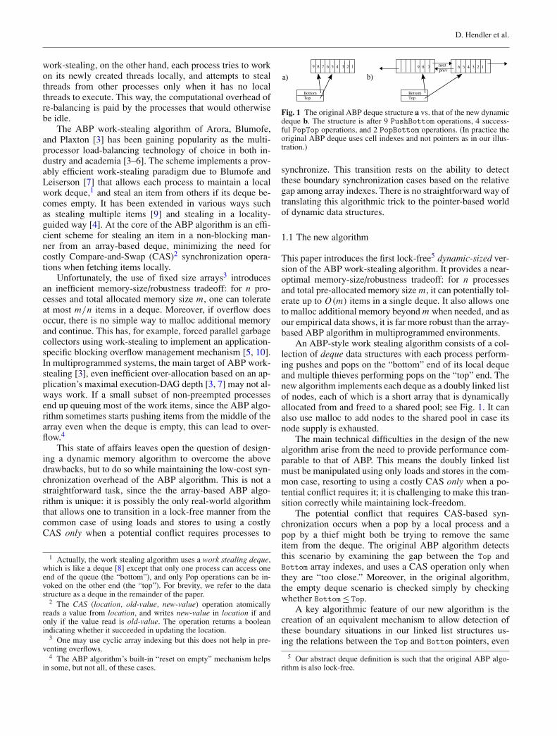
Fig. 1 The original ABP deque structure a vs. that of the new dynamicdeque b. The structure is after 9 PushBottom operations, 4 success-ful PopTop operations, and 2 PopBottom operations. (In practice theoriginal ABP deque uses cell indexes and not pointers as in our illus-tration.)

synchronize. This transition rests on the ability to detectthese boundary synchronization cases based on the relativegap among array indexes. There is no straightforward way oftranslating this algorithmic trick to the pointer-based worldof dynamic data structures.

1.1 The new algorithm

This paper introduces the first lock-free5 dynamic-sized ver-sion of the ABP work-stealing algorithm. It provides a near-optimal memory-size/robustness tradeoff: for n processesand total pre-allocated memory size m, it can potentially tol-erate up to O(m) items in a single deque. It also allows oneto malloc additional memory beyond m when needed, and asour empirical data shows, it is far more robust than the array-based ABP algorithm in multiprogrammed environments.

An ABP-style work stealing algorithm consists of a col-lection of deque data structures with each process perform-ing pushes and pops on the “bottom” end of its local dequeand multiple thieves performing pops on the “top” end. Thenew algorithm implements each deque as a doubly linked listof nodes, each of which is a short array that is dynamicallyallocated from and freed to a shared pool; see Fig. 1. It canalso use malloc to add nodes to the shared pool in case itsnode supply is exhausted.

The main technical difficulties in the design of the newalgorithm arise from the need to provide performance com-parable to that of ABP. This means the doubly linked listmust be manipulated using only loads and stores in the com-mon case, resorting to using a costly CAS only when a po-tential conflict requires it; it is challenging to make this tran-sition correctly while maintaining lock-freedom.

The potential conflict that requires CAS-based syn-chronization occurs when a pop by a local process and apop by a thief might both be trying to remove the sameitem from the deque. The original ABP algorithm detectsthis scenario by examining the gap between the Top andBottom array indexes, and uses a CAS operation only whenthey are “too close.” Moreover, in the original algorithm,the empty deque scenario is checked simply by checkingwhether Bottom≤ Top.

A key algorithmic feature of our new algorithm is thecreation of an equivalent mechanism to allow detection ofthese boundary situations in our linked list structures us-ing the relations between the Top and Bottom pointers, even

5 Our abstract deque definition is such that the original ABP algo-rithm is also lock-free.


though these point to entries that may reside in differentnodes. On a high level, our idea is to prove that one can re-strict the number of possible ways the pointers interact, andtherefore, given one pointer, it is possible to calculate thedifferent possible positions for the other pointer that implysuch a boundary scenario.

The other key feature of our algorithm is that the dy-namic insertion and deletion operations of nodes into thedoubly linked-list (when needed in a push or pop) are per-formed in such a way that the local thread uses only loadsand stores. This contrasts with the more general linked-listdeque implementations [11, 12] which require a double-compare-and-swap synchronization operation [13] to insertand delete nodes.

1.2 Performance analysis

We compared our new dynamic-memory work-stealing al-gorithm to the original ABP algorithm on a 16-node sharedmemory multiprocessor using the benchmarks of the styleused by Blumofe and Papadopoulos [14]. We ran severalstandard Splash2 [15] applications using the Hood scheduler[16] with the ABP and new work-stealing algorithms. Ourresults, presented in Sect. 3, show that the new algorithmperforms as well as ABP, that is, the added dynamic-memoryfeature does not slow the applications down. Moreover, thenew algorithm provides a better memory/robustness ratio:the same amount of memory provides far greater robust-ness in the new algorithm than the original array-basedABP work-stealing. For example, running Barnes-Hut us-ing ABP work-stealing with an 8-fold level of multipro-gramming causes a failure in 40% of the executions ifone uses the deque size that works for stand-alone (non-multiprogrammed) runs. It causes no failures when using thenew dynamic memory work-stealing algorithm.

2 The algorithm

2.1 Basic description

Figure 1b presents our new deque data-structure. Thedoubly-linked list’s nodes are allocated from and freed toa shared pool, and the only case in which one may need tomalloc additional storage is if the shared pool is exhausted.The deque supports the PushBottom and PopBottom opera-tions for the local process, and the PopTop operation for thethieves.

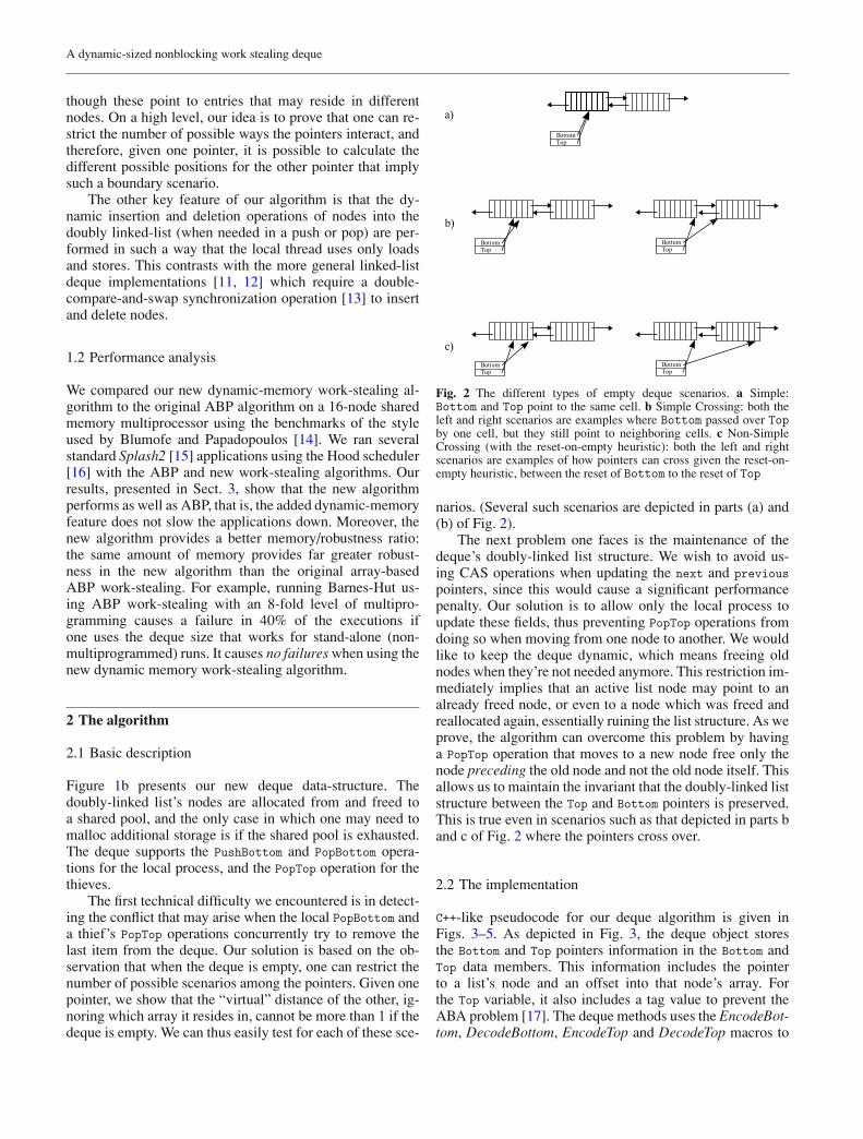
The first technical difficulty we encountered is in detect-ing the conflict that may arise when the local PopBottom anda thief’s PopTop operations concurrently try to remove thelast item from the deque. Our solution is based on the ob-servation that when the deque is empty, one can restrict thenumber of possible scenarios among the pointers. Given onepointer, we show that the “virtual” distance of the other, ig-noring which array it resides in, cannot be more than 1 if thedeque is empty. We can thus easily test for each of these sce-

Fig. 2 The different types of empty deque scenarios. a Simple:Bottom and Top point to the same cell. b Simple Crossing: both theleft and right scenarios are examples where Bottom passed over Topby one cell, but they still point to neighboring cells. c Non-SimpleCrossing (with the reset-on-empty heuristic): both the left and rightscenarios are examples of how pointers can cross given the reset-on-empty heuristic, between the reset of Bottom to the reset of Top

narios. (Several such scenarios are depicted in parts (a) and(b) of Fig. 2).

The next problem one faces is the maintenance of thedeque’s doubly-linked list structure. We wish to avoid us-ing CAS operations when updating the next and previouspointers, since this would cause a significant performancepenalty. Our solution is to allow only the local process toupdate these fields, thus preventing PopTop operations fromdoing so when moving from one node to another. We wouldlike to keep the deque dynamic, which means freeing oldnodes when they’re not needed anymore. This restriction im-mediately implies that an active list node may point to analready freed node, or even to a node which was freed andreallocated again, essentially ruining the list structure. As weprove, the algorithm can overcome this problem by havinga PopTop operation that moves to a new node free only thenode preceding the old node and not the old node itself. Thisallows us to maintain the invariant that the doubly-linked liststructure between the Top and Bottom pointers is preserved.This is true even in scenarios such as that depicted in parts band c of Fig. 2 where the pointers cross over.

2.2 The implementation

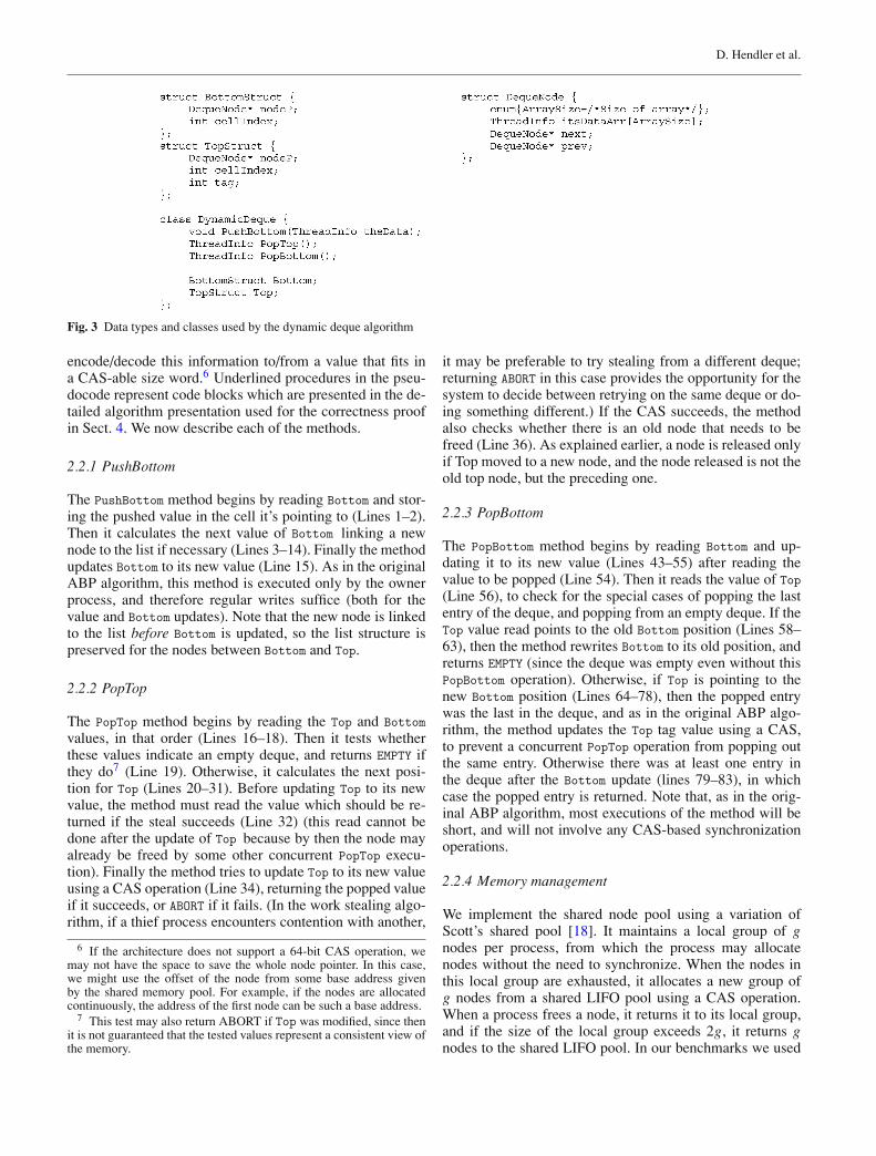
C++-like pseudocode for our deque algorithm is given inFigs. 3–5. As depicted in Fig. 3, the deque object storesthe Bottom and Top pointers information in the Bottom andTop data members. This information includes the pointerto a list’s node and an offset into that node’s array. Forthe Top variable, it also includes a tag value to prevent theABA problem [17]. The deque methods uses the EncodeBot-tom, DecodeBottom, EncodeTop and DecodeTop macros to

D. Hendler et al.

Fig. 3 Data types and classes used by the dynamic deque algorithm

encode/decode this information to/from a value that fits ina CAS-able size word.6 Underlined procedures in the pseu-docode represent code blocks which are presented in the de-tailed algorithm presentation used for the correctness proofin Sect. 4. We now describe each of the methods.

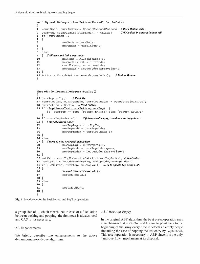
2.2.1 PushBottom

The PushBottom method begins by reading Bottom and stor-ing the pushed value in the cell it’s pointing to (Lines 1–2).Then it calculates the next value of Bottom linking a newnode to the list if necessary (Lines 3–14). Finally the methodupdates Bottom to its new value (Line 15). As in the originalABP algorithm, this method is executed only by the ownerprocess, and therefore regular writes suffice (both for thevalue and Bottom updates). Note that the new node is linkedto the list before Bottom is updated, so the list structure ispreserved for the nodes between Bottom and Top.

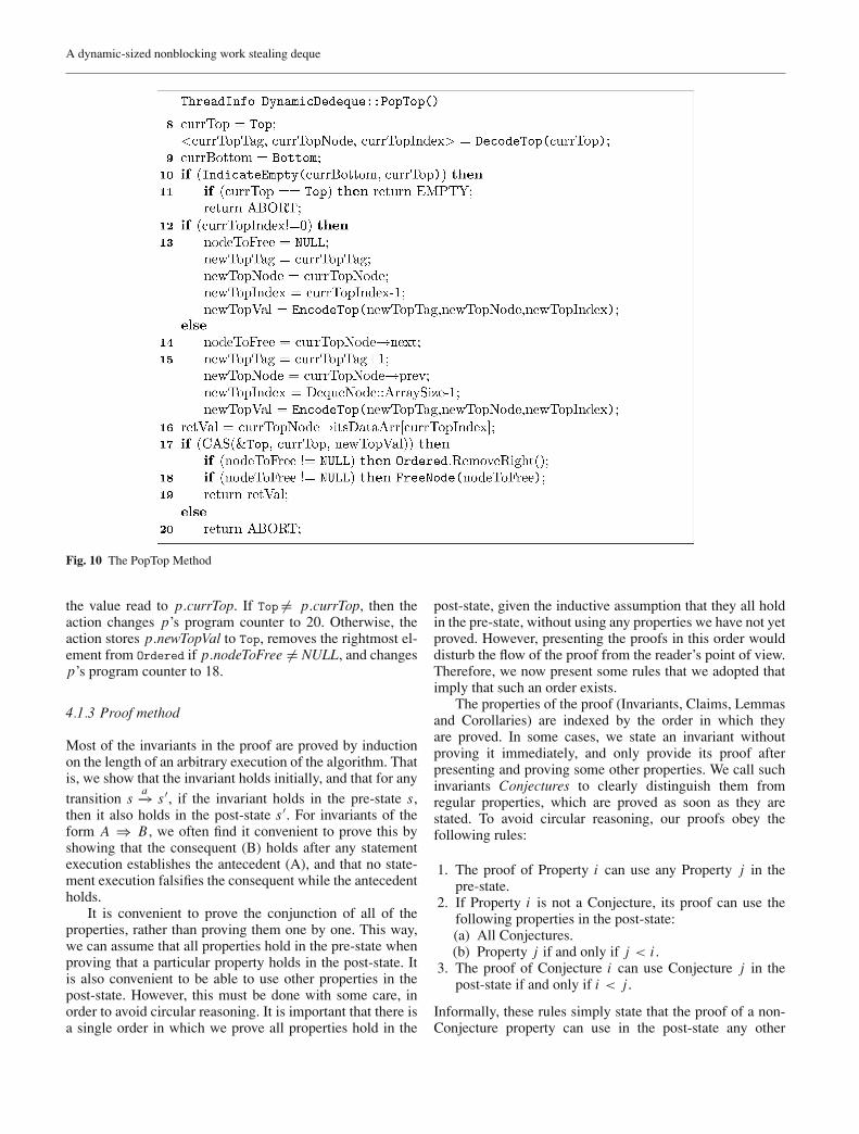
2.2.2 PopTop

The PopTop method begins by reading the Top and Bottomvalues, in that order (Lines 16–18). Then it tests whetherthese values indicate an empty deque, and returns EMPTY ifthey do7 (Line 19). Otherwise, it calculates the next posi-tion for Top (Lines 20–31). Before updating Top to its newvalue, the method must read the value which should be re-turned if the steal succeeds (Line 32) (this read cannot bedone after the update of Top because by then the node mayalready be freed by some other concurrent PopTop execu-tion). Finally the method tries to update Top to its new valueusing a CAS operation (Line 34), returning the popped valueif it succeeds, or ABORT if it fails. (In the work stealing algo-rithm, if a thief process encounters contention with another,

6 If the architecture does not support a 64-bit CAS operation, wemay not have the space to save the whole node pointer. In this case,we might use the offset of the node from some base address givenby the shared memory pool. For example, if the nodes are allocatedcontinuously, the address of the first node can be such a base address.

7 This test may also return ABORT if Top was modified, since thenit is not guaranteed that the tested values represent a consistent view ofthe memory.

it may be preferable to try stealing from a different deque;returning ABORT in this case provides the opportunity for thesystem to decide between retrying on the same deque or do-ing something different.) If the CAS succeeds, the methodalso checks whether there is an old node that needs to befreed (Line 36). As explained earlier, a node is released onlyif Top moved to a new node, and the node released is not theold top node, but the preceding one.

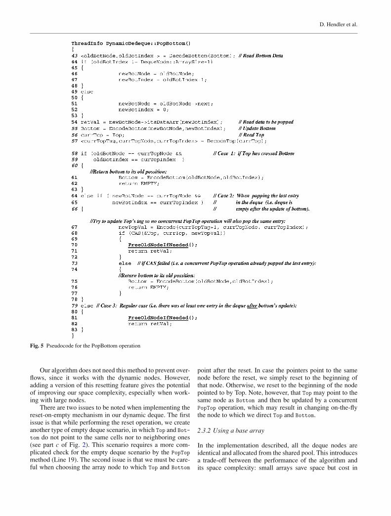
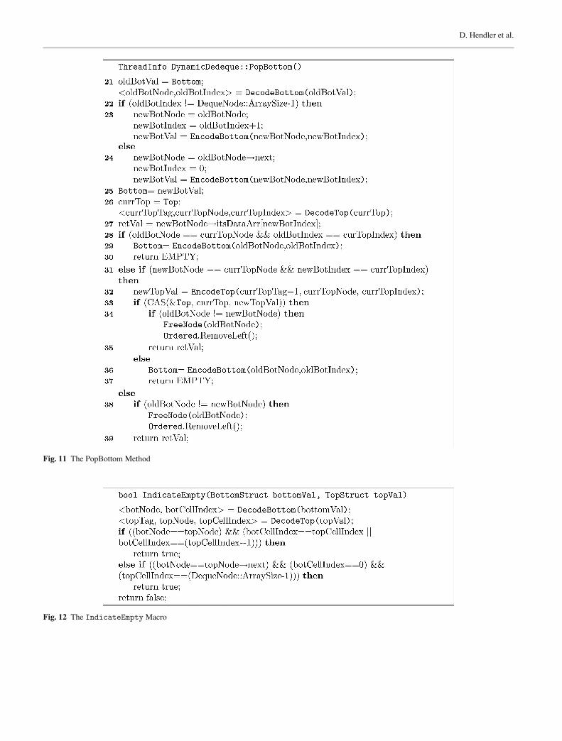
2.2.3 PopBottom

The PopBottom method begins by reading Bottom and up-dating it to its new value (Lines 43–55) after reading thevalue to be popped (Line 54). Then it reads the value of Top(Line 56), to check for the special cases of popping the lastentry of the deque, and popping from an empty deque. If theTop value read points to the old Bottom position (Lines 58–63), then the method rewrites Bottom to its old position, andreturns EMPTY (since the deque was empty even without thisPopBottom operation). Otherwise, if Top is pointing to thenew Bottom position (Lines 64–78), then the popped entrywas the last in the deque, and as in the original ABP algo-rithm, the method updates the Top tag value using a CAS,to prevent a concurrent PopTop operation from popping outthe same entry. Otherwise there was at least one entry inthe deque after the Bottom update (lines 79–83), in whichcase the popped entry is returned. Note that, as in the orig-inal ABP algorithm, most executions of the method will beshort, and will not involve any CAS-based synchronizationoperations.

2.2.4 Memory management

We implement the shared node pool using a variation ofScott’s shared pool [18]. It maintains a local group of gnodes per process, from which the process may allocatenodes without the need to synchronize. When the nodes inthis local group are exhausted, it allocates a new group ofg nodes from a shared LIFO pool using a CAS operation.When a process frees a node, it returns it to its local group,and if the size of the local group exceeds 2g, it returns gnodes to the shared LIFO pool. In our benchmarks we used


Fig. 4 Pseudocode for the PushBottom and PopTop operations

a group size of 1, which means that in case of a fluctuationbetween pushing and popping, the first node is always localand CAS is not necessary.

2.3 Enhancements

We briefly describe two enhancements to the abovedynamic-memory deque algorithm.

2.3.1 Reset-on-Empty

In the original ABP algorithm, the PopBottom operation usesa mechanism that resets Top and Bottom to point back to thebeginning of the array every time it detects an empty deque(including the case of popping the last entry by PopBottom).This reset operation is necessary in ABP since it is the only“anti-overflow” mechanism at its disposal.

D. Hendler et al.

Fig. 5 Pseudocode for the PopBottom operation

Our algorithm does not need this method to prevent over-flows, since it works with the dynamic nodes. However,adding a version of this resetting feature gives the potentialof improving our space complexity, especially when work-ing with large nodes.

There are two issues to be noted when implementing thereset-on-empty mechanism in our dynamic deque. The firstissue is that while performing the reset operation, we createanother type of empty deque scenario, in which Top and Bot-tom do not point to the same cells nor to neighboring ones(see part c of Fig. 2). This scenario requires a more com-plicated check for the empty deque scenario by the PopTopmethod (Line 19). The second issue is that we must be care-ful when choosing the array node to which Top and Bottom

point after the reset. In case the pointers point to the samenode before the reset, we simply reset to the beginning ofthat node. Otherwise, we reset to the beginning of the nodepointed to by Top. Note, however, that Top may point to thesame node as Bottom and then be updated by a concurrentPopTop operation, which may result in changing on-the-flythe node to which we direct Top and Bottom.

2.3.2 Using a base array

In the implementation described, all the deque nodes areidentical and allocated from the shared pool. This introducesa trade-off between the performance of the algorithm andits space complexity: small arrays save space but cost in


allocation overhead, while large arrays cost space but reducethe allocation overhead.

One possible improvement is to use a large array for theinitial base node, allocated for each of the deques, and to usethe pool only when overflow space is needed. This base nodeis used only by the process/deque it was originally allocatedto, and is never freed to the shared pool. Whenever a Popoperation frees this node, it raises a boolean flag, indicatingthat the base node is now free. When a PushBottom operationneeds to allocate and link a new node, it first checks this flag,and if true, links the base node to the deque (instead of aregular node allocated from the shared pool).

3 Performance

We evaluated the performance of the new dynamic mem-ory work-stealing algorithm in comparison to the originalfixed-array based ABP work-stealing algorithm in an envi-ronment similar to that used by Blumofe and Papadopoulos[14] in their evaluation of the ABP algorithm. Our resultsinclude tests running several standard Splash2 [15] appli-cations using the Hood Library [16] on a 16 node SunEnterpriseTM 6500, an SMP machine formed from 8 boardsof two 400MHz UltraSparc� processors, connected by acrossbar UPA switch, and running the SolarisTM 9 operatingsystem.

Our benchmarks used the work-stealing algorithms asthe load balancing mechanism in Hood. The Hood packageuses the original ABP deques for the scheduling of threadsover processes. We compiled two versions of the Hood li-brary, one using an ABP implementation, and the other us-ing the new implementation. In order for the comparison tobe fair, we implemented both algorithms in C++, using thesame tagging method.

We present here our results running the Barnes Hut andMergeSort Splash2 [15] applications. Each application wascompiled with the minimal ABP deque size needed for astand-alone run with the biggest input tested. For our dequealgorithm we chose a base-array size of about 75% of theABP deque size, a node array size of 6 items, and a sharedpool size such that the total memory used (by the deques andthe shared pool together) is no more than the total memoryused by all ABP deques. In all our benchmarks the numberof processes equaled the number of processors on the ma-chine.

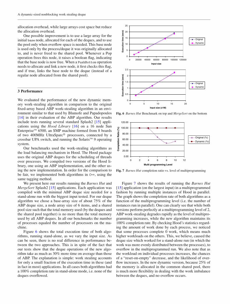
Figure 6 shows the total execution time of both algo-rithms, running stand-alone, as we vary the input size. Ascan be seen, there is no real difference in performance be-tween the two approaches. This is in spite of the fact thatour tests show that the deque operations of the new algo-rithm take as much as 30% more time on average than thoseof ABP. The explanation is simple: work stealing accountsfor only a small fraction of the execution time in these (andin fact in most) applications. In all cases both algorithms hada 100% completion rate in stand-alone mode, i.e. none of thedeques overflowed.

0

5

10

15

20

25

0 20000 40000 60000 80000 100000 120000

Input size

Exe

cuti

on

tim

e (s

ecs)

Original

Dynamic

0

0.5

1

1.5

2

2.5

0 5 10 15 20

Input size (x1M)

Exe

cuti

on

tim

e (s

ecs)

Original

Dynamic

Fig. 6 Barnes Hut Benchmark on top and MergeSort on the bottom

0.00

20.00

40.00

60.00

80.00

100.00

120.00

0 2 4 6 8 10 12

Multi programming Level

Co

mp

leti

on

Rat

io (

%)

Original (%)

Dynamic (%)

Fig. 7 Barnes Hut completion ratio vs. level of multiprogramming

Figure 7 shows the results of running the Barnes Hut[15] application (on the largest input) in a multiprogrammedfashion by running multiple instances of Hood in parallel.The graph shows the completion rate of both algorithms as afunction of the multiprogramming level (i.e. the number ofinstances run in parallel). One can clearly see that while bothversions perform perfectly at a multiprogramming level of 2,ABP work-stealing degrades rapidly as the level of multipro-gramming increases, while the new algorithm maintains its100% completion rate. By checking Hood’s statistics regard-ing the amount of work done by each process, we noticedthat some processes complete 0 work, which means muchhigher workloads on the others. This, we believe, caused thedeque size which worked for a stand-alone run (in which thework was more evenly distributed between the processes), tooverflow in the multiprogrammed run. We also note that asthe workload on individual processes increases, the chancesof a “reset-on-empty” decrease, and the likelihood of over-flow increases. In the new dynamic version, because 25% ofthe memory is allocated in the common shared pool, thereis much more flexibility in dealing with the work imbalancebetween the deques, and no overflow occurs.

D. Hendler et al.

Our preliminary benchmarks clearly show that for thesame amount of memory, we get significantly more robust-ness with the new dynamic algorithm than with the origi-nal ABP algorithm, with a virtually unnoticeable effect onthe application’s overall performance. It also shows that thedeque size depends on the maximal level of multiprogram-ming in the system, an unpredictable parameter which onemay want to avoid reasoning about by simply using the newmemory version of the ABP work stealing algorithm.

4 Correctness proof

4.1 Overview

The full version of this paper [19] contains a detailed proofthat the algorithm in Sect. 2 implements a lock-free lineariz-able deque.8 While a work stealing system generally usesseveral deques, our proof concentrates on a single deque. Forbrevity, this section only contains the outline of the proof.All omitted proofs and claims can be found in the full ver-sion of the paper [19]. To make it easier for the reader, wekept the numbering of the claims the same as in the full ver-sion.

We first define notation and terminology and present adetailed version of the algorithm’s pseudocode that we usethroughout the proof. In Sects. 4.2–4.6 we present variousproperties of the algorithm, which are used later in the lin-earizability proof. Section 4.7 specifies the sequential se-mantics of the implemented deque and then shows that thedeque is linearizable to this specification. Finally, Sect. 4.8shows that the algorithm is lock-free.

4.1.1 Notation

Formally, we model the algorithm by a labelled state-transition system, where the labels are called actions. Wewrite s

a−→ s′ if the system has a transition from s to s′ la-belled a; s is called the pre-state, s′ the post-state. We saythat an action a is enabled in a state s if there exists an-other state s′ such that s

a−→ s′. An execution is a sequenceof transitions such that the pre-state of the first transition isthe initial state, and the post-state of any transition (exceptthe last) is the pre-state of the next transition.

We use s and s′ for states, a for actions, and p, p′ and p′′for processes. We use p@X to mean that process p is readyto execute statement number X. We use p@〈X1, X2, ..., Xn〉to denote p@X1 ∨ p@X2 ∨ ... ∨ p@Xn . If process p is notexecuting any operation then p@0, holds. Thus, p@0 holdsinitially for all p, statements of process that return from anyof the operations establish p@0, and if p@0 holds, thenan action of process p is enabled that nondeterministicallychooses a legal operation and parameters, and invokes the

8 As noted previously, the data structure we implement is not strictlyspeaking a deque. The precise semantics of the implemented datastructure is specified in Sect. 4.7.1.

Fig. 8 Deque Constructor

Fig. 9 The PushBottom Method

operation, thereby setting p’s program counter to the firstline of that operation, and establishing legal values for itsparameters. We denote a private variable v of process p byp.v.

For any variable v, shared or local, s.v denotes the valueof v is state s. For any logical expression E , s.E holds if andonly if E holds in state s.

4.1.2 Pseudocode

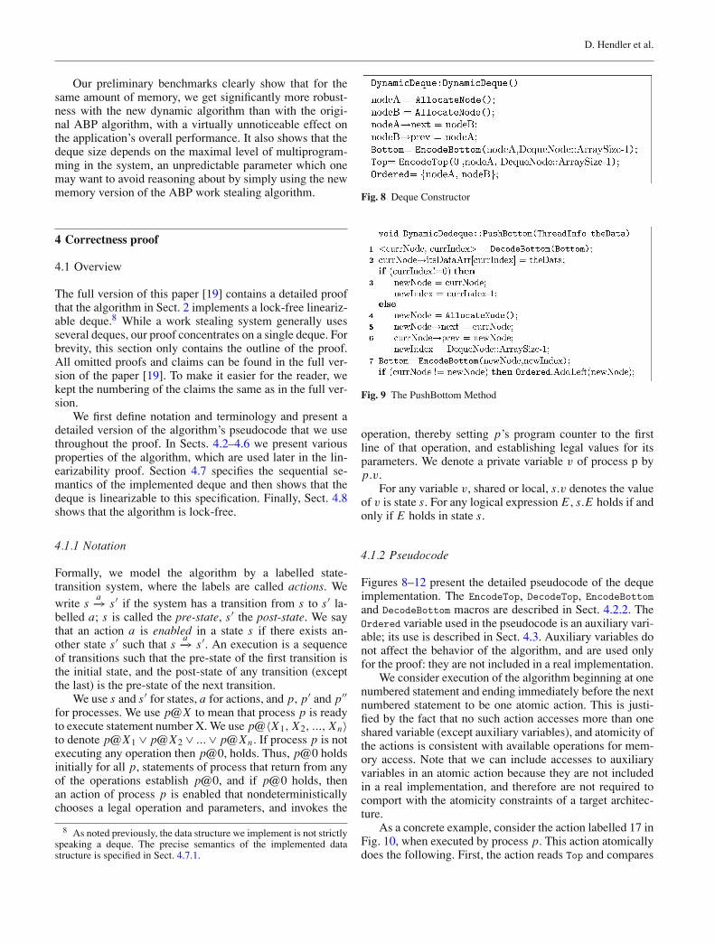
Figures 8–12 present the detailed pseudocode of the dequeimplementation. The EncodeTop, DecodeTop, EncodeBottomand DecodeBottom macros are described in Sect. 4.2.2. TheOrdered variable used in the pseudocode is an auxiliary vari-able; its use is described in Sect. 4.3. Auxiliary variables donot affect the behavior of the algorithm, and are used onlyfor the proof: they are not included in a real implementation.

We consider execution of the algorithm beginning at onenumbered statement and ending immediately before the nextnumbered statement to be one atomic action. This is justi-fied by the fact that no such action accesses more than oneshared variable (except auxiliary variables), and atomicity ofthe actions is consistent with available operations for mem-ory access. Note that we can include accesses to auxiliaryvariables in an atomic action because they are not includedin a real implementation, and therefore are not required tocomport with the atomicity constraints of a target architec-ture.

As a concrete example, consider the action labelled 17 inFig. 10, when executed by process p. This action atomicallydoes the following. First, the action reads Top and compares


Fig. 10 The PopTop Method

the value read to p.currTop. If Top �= p.currTop, then theaction changes p’s program counter to 20. Otherwise, theaction stores p.newTopVal to Top, removes the rightmost el-ement from Ordered if p.nodeToFree �= NULL, and changesp’s program counter to 18.

4.1.3 Proof method

Most of the invariants in the proof are proved by inductionon the length of an arbitrary execution of the algorithm. Thatis, we show that the invariant holds initially, and that for anytransition s

a−→ s′, if the invariant holds in the pre-state s,then it also holds in the post-state s′. For invariants of theform A ⇒ B, we often find it convenient to prove this byshowing that the consequent (B) holds after any statementexecution establishes the antecedent (A), and that no state-ment execution falsifies the consequent while the antecedentholds.

It is convenient to prove the conjunction of all of theproperties, rather than proving them one by one. This way,we can assume that all properties hold in the pre-state whenproving that a particular property holds in the post-state. Itis also convenient to be able to use other properties in thepost-state. However, this must be done with some care, inorder to avoid circular reasoning. It is important that there isa single order in which we prove all properties hold in the

post-state, given the inductive assumption that they all holdin the pre-state, without using any properties we have not yetproved. However, presenting the proofs in this order woulddisturb the flow of the proof from the reader’s point of view.Therefore, we now present some rules that we adopted thatimply that such an order exists.

The properties of the proof (Invariants, Claims, Lemmasand Corollaries) are indexed by the order in which theyare proved. In some cases, we state an invariant withoutproving it immediately, and only provide its proof afterpresenting and proving some other properties. We call suchinvariants Conjectures to clearly distinguish them fromregular properties, which are proved as soon as they arestated. To avoid circular reasoning, our proofs obey thefollowing rules:

1. The proof of Property i can use any Property j in thepre-state.

2. If Property i is not a Conjecture, its proof can use thefollowing properties in the post-state:(a) All Conjectures.(b) Property j if and only if j < i .

3. The proof of Conjecture i can use Conjecture j in thepost-state if and only if i < j .

Informally, these rules simply state that the proof of a non-Conjecture property can use in the post-state any other

D. Hendler et al.

Fig. 11 The PopBottom Method

Fig. 12 The IndicateEmpty Macro


property that was already stated (because the only proper-ties that were stated before it but with higher index are Con-jectures), and that the proof of a Conjecture can use in thepost-state any other Conjecture that was not already proven.In the full version of the paper [19] we show that our proofmethod is sound.

To make the proof more readable, we also avoid using inthe pre-state properties that were not stated yet.

4.2 Basic notation and invariants

4.2.1 The deque data structure

Our deque is implemented using a doubly linked list. Eachlist node contains an array of deque entries. The structure hasBottom and Top variables that indicate cells at the two endsof the deque; these variables are discussed in more detail inSect. 4.2.2. We use the following notation:

• We let N j denote a (pointer to a) deque node, and Cidenotes a cell at index i in a node. Ci ∈ N j denotes thatCi is the i th cell in node N j .

• We let Node(Ci ) denote the node of cell Ci . That is:Node(Ci ) = N j ⇔ Ci ∈ N j .

• The Bottom cell of the deque, denoted by CB , is thecell indicated by Bottom. The Bottom node is the nodein which CB resides, and is denoted by NB .

• The Top cell of the deque, denoted by CT , is the cellindicated by Top. The Top node is the node in which CTresides, and is denoted by NT .

• If N is a deque node, than N → next is the node pointedto by N’s next pointer, and N → prev is the nodepointed to by its previous pointer.

The following property models the assumption thatonly one process calls the PushBottom and PopBottomoperations.

Invariant 1. If p@〈1 . . . 7, 21 . . . 39〉 then:

1. p is the owner process of the deque.2. There is no p′ �= p such that p′@〈1 . . . 7, 21 . . . 39〉.Proof The invariant follows immediately from the require-ment that only the owner process may call the PushBottomor PopBottom procedures. �

4.2.2 The Top and Bottom variables

The Top and Bottom shared variables store information aboutCT and CB , respectively, and they are both of a CASablesize. The Top variable also contains an unbounded Tag value,to avoid the ABA problem as we describe in Sect. 4.2.3. Thestructure of Top and Bottom variables is detailed in Fig. 3.

In practice, in order to store all the information on aCASable word size even if only a 32-bit CAS operation isavailable, we represent the node’s pointer by its offset fromsome base address given by the nodes’ memory manager. In

this case, if the size of the node is of a power of two, wecan even save only the offsets to CT and CB , and calculatethe offsets of NT and NB by simple bitwise operations. Thatway we save the space used by the cellIndex variable, andleave enough space for the tag value.

In the rest of the proof we use the Cell operator to de-note the cell to which a variable of type BottomStruct orTopStruct points (for example, Cell (Top) = CT and Cell(Bottom) = CB):

Definition 3 If TorBVal is a variable of type TopStruct orBottomStruct then: Cell(TorBVal) = TorBVal.nodeP →itsDataArr[TorBVal.cellIndex].

Our implementation uses the EncodeTop and Encode-Bottom macros to construct values of type TopStruct andBottomStruct, respectively, and similarly uses the Decode-Bottom and DecodeTop macros to extract the componentsfrom values of these types. For convenience, we use pro-cesses’ private variables to hold the different fields of valuesread from Top and Bottom. For example, after executing thecode segment:

oldBotVal = Bottom;<oldBotNode,oldBotIndex> = DecodeBottom(oldBotVal);

using oldBotNode and oldBotIndex, as long as they arenot modified, is equivalent to using oldBotVal.nodeP andoldBotVal.cellIndex, respectively.

Invariant 6.

1. p@〈2 . . . 7〉 ⇒ (NB = p.currNode ∧ CB =C p.curr I ndex ∈ NB).

2. p@〈22 . . . 25, 30, 37〉 ⇒ Bottom= p.oldBotVal.3. p@〈26 . . . 29, 31 . . . 36, 38 . . . 39〉 ⇒ Bottom =

p.newBotVal.

4.2.3 The ABA problem

Our implementation uses the CAS operation for all updatesof the Top variable. The CAS synchronization primitive issusceptible to the ABA problem: Assume that the value A isread from some variable v, and later a CAS operation is doneon that variable, with the value A supplied as the old-valueparameter of the CAS. If, between the read and the CAS, thevariable v has been changed to some other value B and thento A again, the CAS would still succeed.

In this section, we prove some properties concerningmechanisms used in the algorithm to avoid the ABA prob-lem. We start by defining an order between different Top val-ues:

Definition 7 Let TopV1 and TopV2 be two values of typeTopStruct. TopV1 � TopV2 if and only if:

1. TopV1.tag ≤ TopV2.tag, and2. (TopV1.tag = TopV2.tag) ⇒ (TopV1.cellIndex >

TopV2.cellIndex).

D. Hendler et al.

Lemma 10 Let sa−→ s′ be a step of the algorithm, and sup-

pose a writes a value to Top. Then s.T op � s′.T op.

Corollary 12 Consider a transition sa−→ s′ where a writes

a value to Top. Then: ∀p s.p@〈9 . . . 20, 27 . . . 39〉 ⇒s′.p.currT op �= s′.T op

4.2.4 Memory management

Our algorithm uses an external linearizable shared poolmodule, which stores the available list nodes. The sharedpool module supports two operations: AllocateNode andFreeNode. The details of the shared pool implementation arenot relevant to our algorithm, so we simply model a lin-earizable shared pool that supports atomic AllocateNode andFreeNode operations.

We model the shared pool using an auxiliary variableLive, which models the set of nodes that have been allocatedfrom the pool and not yet freed:

1. Initially Live= ∅.2. An AllocateNode operation atomically adds a node that

is not in Live to Live and returns that node.3. A FreeNode(N ) operation with N ∈ Liveatomically re-

moves N from Live.4. While N ∈ Live, the shared pool implementation does

not modify any of N ’s fields.

The shared pool behaves according to the above rulesprovided our algorithm uses it properly. The following con-jecture states the rules for proper use of the shared pool. Weprove that the conjecture holds in Sect. 4.4.

Conjecture 30. Consider a transition sa−→ s′ of our algo-

rithm.

• If N /∈ s.Live, then a does not modify any of N ’s fields.• If a is an execution of FreeNode(N ), then N ∈ s.Live.

Definition 13 A node N is live if and only if N ∈ Live.

4.3 Ordered nodes

We introduce an auxiliary variable Ordered, which consistsof a sequence of nodes. We regard the order of the nodesin Ordered as going from left to right. Formally, the vari-able Ordered supports four operations: AddLeft, AddRight,RemoveLeft and RemoveRight. If |Ordered| = l, Ordered={N1, . . . , Nl} then:

• N1 is the leftmost node and Nl is the rightmost one.• An Ordered.AddLeft(N) operation results in Ordered=

{N , N1, . . . , Nl}.• An Ordered.AddRight(N) operation results in Ordered=

{N1, . . . , Nl , N }.• A Ordered.RemoveLeft() operation results in Ordered=

{N2, . . . , Nl}, and returns N1.• A Ordered.RemoveRight() operation results in Ordered

= {N1, . . . , Nl−1}, and returns Nl .

Definition 14 A node N is ordered if and only if N ∈Ordered.

The following conjecture describes the basic properties ofthe nodes in Ordered:

Conjecture 55. Let |Ordered| = n + 2, Ordered= {N0,. . . , Nn+1}. Then:

1. ∀0≤i≤n Ni → next = Ni+1 ∧ Ni+1 → prev = Ni .2. Exactly one of the following holds:

(a) n ≥ 0, N0 = NB, Nn = NT .(b) n > 0, N1 = NB, Nn = NT .(c) n = 0, N0 = NT , N1 = NB .

Corollary 15

1. |s.Ordered| ≥ 2.2. NT is ordered and is the second node from the right in

Ordered.3. NB is ordered and is either the first or the second node

from the left in Ordered.4. NT → next is Ordered.

Proof Straightforward from Conjecture 55. � The following invariants and lemmas state different proper-ties of the nodes in Ordered.

Invariant 16. Exactly one of the following holds:

1. NB is the leftmost node in Ordered ∧(p@〈26 . . . 34, 36 . . . 38〉 ⇒ p.oldBotNode = NB).

2. ∃p such that p@〈26 . . . 29, 31 . . . 34, 36, 38〉∧ NB �=p.oldBotNode ∧ p.oldBotNode is the leftmost node inOrdered.

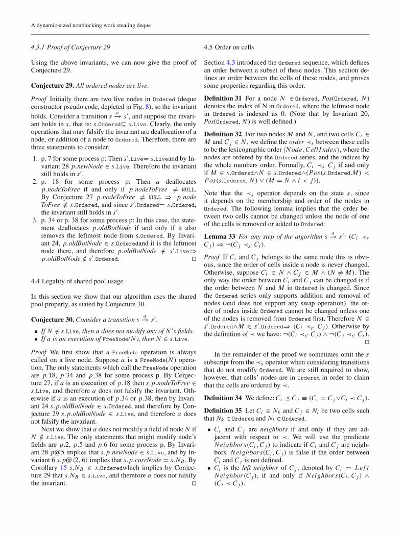
Conjecture 29. All ordered nodes are live.

We now present various properties about the ordered nodes,which we use later to prove Conjecture 29. The proof ofConjecture 29 appears in Sect. 4.3.1.

Invariant 20. Suppose Ordered = {N0, . . . Nn+1}. Then∀0≤i, j≤n+1, i �= j ⇒ Ni �= N j .

Invariant 24. If p@〈22 . . . 34, 36 . . . 38〉 then p.oldBotNode ∈ Ordered, and it is the leftmost node there.

Invariant 25. If p@〈5 . . . 7〉 ∧ p′@18 ∧ p′ �= p ∧p′.nodeToFree �= NULL then p.newNode �= p′.nodeToFree.

Invariant 26. If p@18 ∧ p′@18, then (p′.nodeToFree �=p.nodeToFree)∨ (p.nodeToFree = p′.nodeToFree = NULL).

Conjecture 27. If p@18 ∧ p.nodeToFree �= NULL thenp.nodeToFree ∈ Live ∧p.nodeToFree /∈ Ordered.

Invariant 28. If p@〈5 . . . 7〉, then p.newNode ∈ Live.


4.3.1 Proof of Conjecture 29

Using the above invariants, we can now give the proof ofConjecture 29.

Conjecture 29. All ordered nodes are live.

Proof Initially there are two live nodes in Ordered (dequeconstructor pseudo code, depicted in Fig. 8), so the invariantholds. Consider a transition s

a−→ s′, and suppose the invari-ant holds in s, that is: s.Ordered⊆ s.Live. Clearly, the onlyoperations that may falsify the invariant are deallocation of anode, or addition of a node to Ordered. Therefore, there arethree statements to consider:

1. p. 7 for some process p: Then s′.Live= s.Liveand by In-variant 28 p.newNode ∈ s.Live. Therefore the invariantstill holds in s′.

2. p. 18 for some process p: Then a deallocatesp.nodeToFree if and only if p.nodeToFree �= NULL.By Conjecture 27 p.nodeToFree �= NULL ⇒ p.nodeToFree /∈ s.Ordered, and since s′.Ordered= s.Ordered,the invariant still holds in s′.

3. p. 34 or p. 38 for some process p: In this case, the state-ment deallocates p.oldBotNode if and only if it alsoremoves the leftmost node from s.Ordered. By Invari-ant 24, p.oldBotNode ∈ s.Orderedand it is the leftmostnode there, and therefore p.oldBotNode /∈ s′.Live⇒p.oldBotNode /∈ s′.Ordered. �

4.4 Legality of shared pool usage

In this section we show that our algorithm uses the sharedpool properly, as stated by Conjecture 30.

Conjecture 30. Consider a transition sa−→ s′.

• If N /∈ s.Live, then a does not modify any of N’s fields.• If a is an execution of FreeNode(N), then N ∈ s.Live.

Proof We first show that a FreeNode operation is alwayscalled on a live node. Suppose a is a FreeNode(N ) opera-tion. The only statements which call the FreeNode operationare p.18, p.34 and p.38 for some process p. By Conjec-ture 27, if a is an execution of p.18 then s.p.nodeToFree ∈s.Live, and therefore a does not falsify the invariant. Oth-erwise if a is an execution of p.34 or p.38, then by Invari-ant 24 s.p.oldBotNode ∈ s.Ordered, and therefore by Con-jecture 29 s.p.oldBotNode ∈ s.Live, and therefore a doesnot falsify the invariant.

Next we show that a does not modify a field of node N ifN /∈ s.Live. The only statements that might modify node’sfields are p.2, p.5 and p.6 for some process p. By Invari-ant 28 p@5 implies that s.p.newNode ∈ s.Live, and by In-variant 6 s.p@〈2, 6〉 implies that s.p.currNode = s.NB . ByCorollary 15 s.NB ∈ s.Orderedwhich implies by Conjec-ture 29 that s.NB ∈ s.Live, and therefore a does not falsifythe invariant. �

4.5 Order on cells

Section 4.3 introduced the Ordered sequence, which definesan order between a subset of these nodes. This section de-fines an order between the cells of these nodes, and provessome properties regarding this order.

Definition 31 For a node N ∈ Ordered, Pos(Ordered, N )denotes the index of N in Ordered, where the leftmost nodein Ordered is indexed as 0. (Note that by Invariant 20,Pos(Ordered, N ) is well defined.)

Definition 32 For two nodes M and N , and two cells Ci ∈M and C j ∈ N , we define the order ≺s between these cellsto be the lexicographic order 〈Node, Cell I ndex〉, where thenodes are ordered by the Ordered series, and the indices bythe whole numbers order. Formally, Ci ≺s C j if and onlyif M ∈ s.Ordered∧N ∈ s.Ordered∧(Pos(s.Ordered,M) <Pos(s.Ordered, N ) ∨ (M = N ∧ i < j)).

Note that the ≺s operator depends on the state s, sinceit depends on the membership and order of the nodes inOrdered. The following lemma implies that the order be-tween two cells cannot be changed unless the node of oneof the cells is removed or added to Ordered:

Lemma 33 For any step of the algorithm sa−→ s′: (Ci ≺s

C j ) ⇒ ¬(C j ≺s′ Ci ).

Proof If Ci and C j belongs to the same node this is obvi-ous, since the order of cells inside a node is never changed.Otherwise, suppose Ci ∈ N ∧ C j ∈ M ∧ (N �= M). Theonly way the order between Ci and C j can be changed is ifthe order between N and M in Ordered is changed. Sincethe Ordered series only supports addition and removal ofnodes (and does not support any swap operation), the or-der of nodes inside Ordered cannot be changed unless oneof the nodes is removed from Ordered first. Therefore N ∈s′.Ordered∧M ∈ s′.Ordered⇒ (Ci ≺s′ C j ). Otherwise bythe definition of ≺ we have: ¬(Ci ≺s′ C j ) ∧ ¬(C j ≺s′ Ci ).

� In the remainder of the proof we sometimes omit the s

subscript from the ≺s operator when considering transitionsthat do not modify Ordered. We are still required to show,however, that cells’ nodes are in Ordered in order to claimthat the cells are ordered by ≺.

Definition 34 We define: Ci � C j ≡ (Ci = C j ∨Ci ≺ C j ).

Definition 35 Let Ci ∈ Nk and C j ∈ Nl be two cells suchthat Nk ∈ Ordered and Nl ∈ Ordered.

• Ci and C j are neighbors if and only if they are ad-jacent with respect to ≺. We will use the predicateNeighbors(Ci , C j ) to indicate if Ci and C j are neigh-bors. Neighbors(Ci , C j ) is false if the order betweenCi and C j is not defined.

• Ci is the left neighbor of C j , denoted by Ci = Le f tNeighbor(C j ), if and only if Neighbors(Ci , C j ) ∧(Ci ≺ C j ).

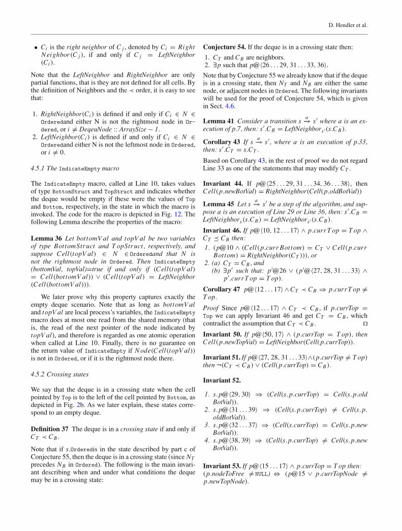
D. Hendler et al.

• Ci is the right neighbor of C j , denoted by Ci = RightNeighbor(C j ), if and only if C j = LeftNeighbor(Ci ).

Note that the LeftNeighbor and RightNeighbor are onlypartial functions, that is they are not defined for all cells. Bythe definition of Neighbors and the ≺ order, it is easy to seethat:

1. RightNeighbor(Ci ) is defined if and only if Ci ∈ N ∈Orderedand either N is not the rightmost node in Or-dered, or i �= DeqeuNode :: ArraySize − 1.

2. LeftNeighbor(Ci ) is defined if and only if Ci ∈ N ∈Orderedand either N is not the leftmost node in Ordered,or i �= 0.

4.5.1 The IndicateEmpty macro

The IndicateEmpty macro, called at Line 10, takes valuesof type BottomStruct and TopStruct and indicates whetherthe deque would be empty if these were the values of Topand Bottom, respectively, in the state in which the macro isinvoked. The code for the macro is depicted in Fig. 12. Thefollowing Lemma describe the properties of the macro:

Lemma 36 Let bottomV al and topV al be two variablesof type BottomStruct and T opStruct, respectively, andsuppose Cell(topV al) ∈ N ∈ Orderedand that N isnot the rightmost node in Ordered. Then IndicateEmpty(bottomVal, topVal)=true if and only if (Cell(topV al)= Cell(bottomV al)) ∨ (Cell(topV al) = LeftNeighbor(Cell(bottomV al))).

We later prove why this property captures exactly theempty deque scenario. Note that as long as bottomV aland topV al are local process’s variables, the IndicateEmptymacro does at most one read from the shared memory (thatis, the read of the next pointer of the node indicated bytopV al), and therefore is regarded as one atomic operationwhen called at Line 10. Finally, there is no guarantee onthe return value of IndicateEmpty if Node(Cell(topV al))is not in Ordered, or if it is the rightmost node there.

4.5.2 Crossing states

We say that the deque is in a crossing state when the cellpointed by Top is to the left of the cell pointed by Bottom, asdepicted in Fig. 2b. As we later explain, these states corre-spond to an empty deque.

Definition 37 The deque is in a crossing state if and only ifCT ≺ CB .

Note that if s.Orderedis in the state described by part c ofConjecture 55, then the deque is in a crossing state (since NTprecedes NB in Ordered). The following is the main invari-ant describing when and under what conditions the dequemay be in a crossing state:

Conjecture 54. If the deque is in a crossing state then:

1. CT and CB are neighbors.2. ∃p such that p@〈26 . . . 29, 31 . . . 33, 36〉.Note that by Conjecture 55 we already know that if the dequeis in a crossing state, then NT and NB are either the samenode, or adjacent nodes in Ordered. The following invariantswill be used for the proof of Conjecture 54, which is givenin Sect. 4.6.

Lemma 41 Consider a transition sa−→ s′ where a is an ex-

ecution of p.7, then: s′.CB = LeftNeighbors′(s.CB).

Corollary 43 If sa−→ s′, where a is an execution of p.33,

then: s′.CT = s.CT .

Based on Corollary 43, in the rest of proof we do not regardLine 33 as one of the statements that may modify CT .

Invariant 44. If p@〈25 . . . 29, 31 . . . 34, 36 . . . 38〉, thenCell(p.newBotVal) = RightNeighbor(Cell(p.oldBotVal))

Lemma 45 Let sa−→ s′ be a step of the algorithm, and sup-

pose a is an execution of Line 29 or Line 36, then: s′.CB =LeftNeighbors(s.CB) = LeftNeighbors′(s.CB).

Invariant 46. If p@〈10, 12 . . . 17〉 ∧ p.currT op = T op ∧CT � CB then:

1. (p@10 ∧ (Cell(p.curr Bottom) = CT ∨ Cell(p.currBottom) = RightNeighbor(CT ))), or

2. (a) CT = CB, and(b) ∃p′ such that: p′@26 ∨ (p′@〈27, 28, 31 . . . 33〉 ∧

p′.currT op = T op).

Corollary 47 p@〈12 . . . 17〉 ∧ CT ≺ CB ⇒ p.currT op �=T op.

Proof Since p@〈12 . . . 17〉 ∧ CT ≺ CB , if p.currTop =Top we can apply Invariant 46 and get CT = CB , whichcontradict the assumption that CT ≺ CB . � Invariant 50. If p@〈50, 17〉 ∧ (p.currTop = T op), thenCell(p.newTopVal) = LeftNeighbor(Cell(p.currTop)).

Invariant 51. If p@〈27, 28, 31 . . . 33〉∧(p.currTop �= T op)then ¬(CT ≺ CB) ∨ (Cell(p.currTop) = CB).

Invariant 52.

1. s.p@〈29, 30〉 ⇒ (Cell(s.p.currTop) = Cell(s.p.oldBotVal)).

2. s.p@〈31 . . . 39〉 ⇒ (Cell(s.p.currTop) �= Cell(s.p.oldBotVal)).

3. s.p@〈32 . . . 37〉 ⇒ (Cell(s.currTop) = Cell(s.p.newBotVal)).

4. s.p@〈38, 39〉 ⇒ (Cell(s.p.currTop) �= Cell(s.p.newBotVal)).

Invariant 53. If p@〈15 . . . 17〉 ∧ p.currTop = T op then:(p.nodeToFree �= NULL) ⇔ (p@15 ∨ p.currTopNode �=p.newTopNode).


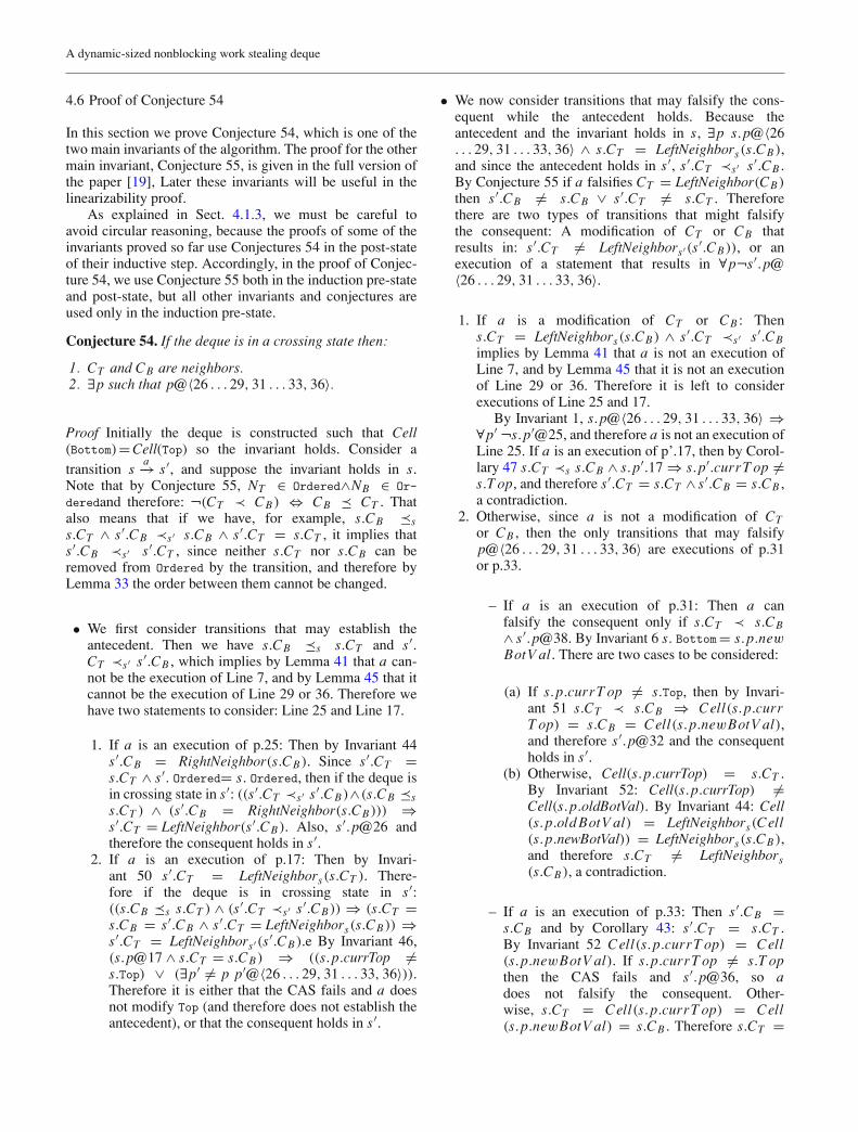
4.6 Proof of Conjecture 54

In this section we prove Conjecture 54, which is one of thetwo main invariants of the algorithm. The proof for the othermain invariant, Conjecture 55, is given in the full version ofthe paper [19], Later these invariants will be useful in thelinearizability proof.

As explained in Sect. 4.1.3, we must be careful toavoid circular reasoning, because the proofs of some of theinvariants proved so far use Conjectures 54 in the post-stateof their inductive step. Accordingly, in the proof of Conjec-ture 54, we use Conjecture 55 both in the induction pre-stateand post-state, but all other invariants and conjectures areused only in the induction pre-state.

Conjecture 54. If the deque is in a crossing state then:

1. CT and CB are neighbors.2. ∃p such that p@〈26 . . . 29, 31 . . . 33, 36〉.

Proof Initially the deque is constructed such that Cell(Bottom) = Cell(Top) so the invariant holds. Consider atransition s

a−→ s′, and suppose the invariant holds in s.Note that by Conjecture 55, NT ∈ Ordered∧NB ∈ Or-deredand therefore: ¬(CT ≺ CB) ⇔ CB � CT . Thatalso means that if we have, for example, s.CB �ss.CT ∧ s′.CB ≺s′ s.CB ∧ s′.CT = s.CT , it implies thats′.CB ≺s′ s′.CT , since neither s.CT nor s.CB can beremoved from Ordered by the transition, and therefore byLemma 33 the order between them cannot be changed.

• We first consider transitions that may establish theantecedent. Then we have s.CB �s s.CT and s′.CT ≺s′ s′.CB , which implies by Lemma 41 that a can-not be the execution of Line 7, and by Lemma 45 that itcannot be the execution of Line 29 or 36. Therefore wehave two statements to consider: Line 25 and Line 17.

1. If a is an execution of p.25: Then by Invariant 44s′.CB = RightNeighbor(s.CB). Since s′.CT =s.CT ∧ s′. Ordered= s. Ordered, then if the deque isin crossing state in s′: ((s′.CT ≺s′ s′.CB)∧(s.CB �ss.CT ) ∧ (s′.CB = RightNeighbor(s.CB))) ⇒s′.CT = LeftNeighbor(s′.CB). Also, s′.p@26 andtherefore the consequent holds in s′.

2. If a is an execution of p.17: Then by Invari-ant 50 s′.CT = LeftNeighbors(s.CT ). There-fore if the deque is in crossing state in s′:((s.CB �s s.CT ) ∧ (s′.CT ≺s′ s′.CB)) ⇒ (s.CT =s.CB = s′.CB ∧ s′.CT = LeftNeighbors(s.CB)) ⇒s′.CT = LeftNeighbors′(s′.CB).e By Invariant 46,(s.p@17 ∧ s.CT = s.CB) ⇒ ((s.p.currTop �=s.Top) ∨ (∃p′ �= p p′@〈26 . . . 29, 31 . . . 33, 36〉)).Therefore it is either that the CAS fails and a doesnot modify Top (and therefore does not establish theantecedent), or that the consequent holds in s′.

• We now consider transitions that may falsify the cons-equent while the antecedent holds. Because theantecedent and the invariant holds in s, ∃p s.p@〈26. . . 29, 31 . . . 33, 36〉 ∧ s.CT = LeftNeighbors(s.CB),and since the antecedent holds in s′, s′.CT ≺s′ s′.CB .By Conjecture 55 if a falsifies CT = LeftNeighbor(CB)then s′.CB �= s.CB ∨ s′.CT �= s.CT . Thereforethere are two types of transitions that might falsifythe consequent: A modification of CT or CB thatresults in: s′.CT �= LeftNeighbors′(s′.CB)), or anexecution of a statement that results in ∀p¬s′.p@〈26 . . . 29, 31 . . . 33, 36〉.

1. If a is a modification of CT or CB : Thens.CT = LeftNeighbors(s.CB) ∧ s′.CT ≺s′ s′.CBimplies by Lemma 41 that a is not an execution ofLine 7, and by Lemma 45 that it is not an executionof Line 29 or 36. Therefore it is left to considerexecutions of Line 25 and 17.

By Invariant 1, s.p@〈26 . . . 29, 31 . . . 33, 36〉 ⇒∀p′ ¬s.p′@25, and therefore a is not an execution ofLine 25. If a is an execution of p’.17, then by Corol-lary 47 s.CT ≺s s.CB ∧ s.p′.17 ⇒ s.p′.currT op �=s.T op, and therefore s′.CT = s.CT ∧ s′.CB = s.CB ,a contradiction.

2. Otherwise, since a is not a modification of CTor CB , then the only transitions that may falsifyp@〈26 . . . 29, 31 . . . 33, 36〉 are executions of p.31or p.33.

– If a is an execution of p.31: Then a canfalsify the consequent only if s.CT ≺ s.CB∧ s′.p@38. By Invariant 6 s. Bottom= s.p.newBotV al. There are two cases to be considered:

(a) If s.p.currT op �= s.Top, then by Invari-ant 51 s.CT ≺ s.CB ⇒ Cell(s.p.currT op) = s.CB = Cell(s.p.newBotV al),and therefore s′.p@32 and the consequentholds in s′.

(b) Otherwise, Cell(s.p.currTop) = s.CT .By Invariant 52: Cell(s.p.currTop) �=Cell(s.p.oldBotVal). By Invariant 44: Cell(s.p.old BotV al) = LeftNeighbors(Cell(s.p.newBotVal)) = LeftNeighbors(s.CB),and therefore s.CT �= LeftNeighbors(s.CB), a contradiction.

– If a is an execution of p.33: Then s′.CB =s.CB and by Corollary 43: s′.CT = s.CT .By Invariant 52 Cell(s.p.currT op) = Cell(s.p.newBotV al). If s.p.currT op �= s.T opthen the CAS fails and s′.p@36, so adoes not falsify the consequent. Other-wise, s.CT = Cell(s.p.currT op) = Cell(s.p.newBotV al) = s.CB . Therefore s.CT =

D. Hendler et al.

s.CB , which implies s′.CT = s′.CB , so theantecedent does not hold in s′. �

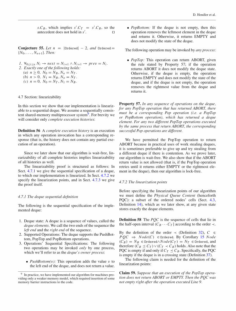
Conjecture 55. Let n = |Ordered| − 2, and Ordered={N0, . . . , Nn+1}. Then:

1. ∀0≤i≤n Ni → next = Ni+1 ∧ Ni+1 → prev = Ni .2. Exactly one of the following holds:

(a) n ≥ 0, N0 = NB, Nn = NT .(b) n > 0, N1 = NB, Nn = NT .(c) n = 0, N0 = NT , N1 = NB.

4.7 Section: linearizability

In this section we show that our implementation is lineariz-able to a sequential deque. We assume a sequentially consis-tent shared-memory multiprocessor system9. For brevity wewill consider only complete execution histories:

Definition 56 A complete execution history is an executionin which any operation invocation has a corresponding re-sponse (that is, the history does not contain any partial exe-cution of an operation).

Since we later show that our algorithm is wait-free, lin-earizability of all complete histories implies linearizabilityof all histories as well.

The linearizability proof is structured as follows: InSect. 4.7.1 we give the sequential specification of a deque,to which our implementation is linearized. In Sect. 4.7.2 wespecify the linearization points, and in Sect. 4.7.3 we givethe proof itself.

4.7.1 The deque sequential definition

The following is the sequential specification of the imple-mented deque:

1. Deque state: A deque is a sequence of values, called thedeque elements. We call the two ends of the sequence theleft end and the right end of the sequence.

2. Supported Operations: The deque supports the PushBot-tom, PopTop and PopBottom operations.

3. Operations’ Sequential Specifications: The followingtwo operations may be invoked only by one process,which we’ll refer to as the deque’s owner process:

• PushBottom(v): This operation adds the value v tothe left end of the deque, and does not return a value.

9 In practice, we have implemented our algorithm for machines pro-viding only a weaker memory model, which required insertion of somememory barrier instructions to the code.

• PopBottom: If the deque is not empty, then thisoperation removes the leftmost element in the dequeand returns it. Otherwise, it returns EMPTY anddoes not modify the state of the deque.

The following operation may be invoked by any process:

• PopTop: This operation can return ABORT, giventhe rule stated by Property 57; if the operationreturns ABORT it does not modify the deque state.Otherwise, if the deque is empty, the operationreturns EMPTY and does not modify the state of thedeque, and if the deque is not empty, the operationremoves the rightmost value from the deque andreturns it.

Property 57. In any sequence of operations on the deque,for any PopTop operation that has returned ABORT, theremust be a corresponding Pop operation (i.e. a PopTopor PopBottom operation), which has returned a dequeelement. For any two different PopTop operations executedby the same process that return ABORT, the correspondingsuccessful Pop operations are different.

We have permitted the PopTop operation to returnABORT because in practical uses of work stealing deques,it is sometimes preferable to give up and try stealing froma different deque if there is contention. As we prove later,our algorithm is wait-free. We also show that if the ABORTreturn value is not allowed (that is, if the PopTop operationretries until it returns either EMPTY or the rightmost ele-ment in the deque), then our algorithm is lock-free.

4.7.2 The linearization points

Before specifying the linearization points of our algorithmwe must define the Physical Queue Content (henceforthPQC): a subset of the ordered nodes’ cells (Sect. 4.3,Definition 14), which as we later show, at any given statestores exactly the deque elements.

Definition 58 The PQC is the sequence of cells that lie inthe half-open interval (CB · · · CT ] according to the order ≺.

By the definition of the order ≺ (Definition 32), C ∈P QC ⇒ Node(C) ∈ Ordered. By Corollary 15 Node(CB) = NB ∈ Ordered∧Node(CT ) = NT ∈ Ordered, andtherefore (CB � CT )∨ (CT ≺ CB) holds. Also note that thePQC is empty if and only if CT � CB . Specifically, the PQCis empty if the deque is in a crossing state (Definition 37).

The following claim is needed for the definition of thelinearization points:

Claim 59. Suppose that an execution of the PopTop opera-tion does not return ABORT or EMPTY. Then the PQC wasnot empty right after the operation executed Line 9.


Definition 60 Linearization Points:

PushBottom The linearization point of this method is theupdate of Bottom at Line 7.

PopBottom The linearization point of this method dependson its returned value, as follows:

• EMPTY: The linearization point here is the read of Topat Line 26.

• A deque entry: The linearization point here is the up-date of Bottom at Line 25.

PopTop The linearization point of this method depends onits return value, as follows:

• EMPTY: The linearization point here is the read ofBottom pointer at Line 9.

• ABORT: The linearization point here is the statementthat first observed the modification of Top. This is ei-ther the CAS operation at Line 17, or the read of Topat Line 11.

• A deque entry: If the PQC was not empty right beforethe CAS statement at Line 17, then the linearizationpoint is that CAS statement. Otherwise, it is the firststatement whose execution modified the PQC to beempty, in the interval after the execution of 9, andright before the execution of the CAS operation atLine 17.10

Claim 61. The linearization points of the algorithm are welldefined. That is, for any PushBottom, PopTop, or PopBot-tom operation, the linearization point statement is executedbetween the invocation and response of that operation.

Proof By examination of the code, all the linearizationpoints except the one of a PopTop operation that returns adeque entry are well defined, since they are statements thatare always executed by the operation being linearized. In thecase of a PopTop operation, if the linearization point is theCAS statement, then it is obvious. Otherwise, the PQC wasempty right before the execution of this successful CAS op-eration, and by Claim 57 the PQC was not empty right afterthe PopTop operation executed Line 9. Therefore there musthave been a transition that modified the PQC to be empty inthis interval, and this transition corresponds to the lineariza-tion point of the PopTop operation. � 4.7.3 The linearizability proof

In this section we show that our implementation is lin-earizable to the sequential deque specification given inSect. 4.7.1. For this we need several lemmas, including onethat shows how the linearization points of the deque opera-tions modify the PQC, and one that shows that the PQC isnot modified except at the linearization point of some oper-ation.

10 Note that the linearization point of the PopTop operation in thiscase might be the execution of a statement by a process other then theone executing the linearized PopTop operation. The existence of thispoint is justified in Claim 59.

Lemma 64 Consider a transition sa−→ s′ where a is a state-

ment execution corresponding to a linearization point of adeque operation. Then:

• Case 1: If a is the linearization point of a PushBottom(v)operation, then it adds a cell containing v to the left endof the PQC.

• Case 2: If a is the linearization point of a PopBottomoperation: let R be the operation returned value:11

– If R is EMPTY, then the s.P QC = s′.P QC = ∅.– If R is a deque entry, then R is stored in the leftmost

cell of s.P QC, and this cell does not belong tos′.P QC.

• Case 3: If a is the linearization point of a PopTopoperation: let R be the operation return value:

– If R is EMPTY, then the s.P QC = s′.P QC = ∅.– If R is a deque entry, then R is stored in the right-

most cell of s.P QC, and this cell does not belong tos′.P QC.

Definition 68 A successful Pop operation is either a Pop-Top or a PopBottom operation that did not return EMPTYor ABORT.

Lemma 69 Consider a transition sa−→ s′ that modifies the

PQC (that is, s.P QC �= s′.P QC), then a is the executionof a linearization point of either a PushBottom operation, aPopBottom operation, or a successful PopTop operation.

The following lemma shows that the ABORT propertyholds:

Lemma 70 In any complete execution history, for any Pop-Top operation that has returned ABORT, there is a corre-sponding Pop operation (that is, a PopTop or PopBottom op-eration), which has returned a deque element. For any twodifferent PopTop operations executed by the same processthat returned ABORT, the corresponding successful Pop op-erations are different.

The Linearizablity Theorem: Using Lemmas 64, 69,and 70, we now show that our implementation is linearizableto the sequential deque specification given in Sect. 4.7.1:

Theorem 71 Any complete execution history of our algo-rithm is linearizable to the sequential deque specificationgiven in Sect. 4.7.1.

Proof Given an arbitrary complete execution history of thealgorithm, we construct a total order of the deque operationsby ordering them in the order of their linearization points.By Claim 61, each operation’s linearization point occurs af-ter it is invoked and before it returns, and therefore the total

11 We can refer to the returned value of an operation since we’re deal-ing only with complete histories.

D. Hendler et al.

order defined respects the partial order in the concurrent ex-ecution.

It is left to show that the sequence of operations inthat total order respects the sequential specification given inSect. 4.7.1. We begin with some notation. For each state sin the execution, we assign an abstract deque state, which isachieved by starting with an empty abstract deque, and ap-plying to it all of the operations whose linearization pointsoccurs before s in the order in which they occur in the exe-cution.

We say that the PQC sequence matches the abstractdeque sequence in a state s, if and only if the length ofthe abstract deque state and the length of the PQC (denotedlength(PQC)) are equal, and for all i ∈ [0..length(P QC)),the data stored in the ith cell of the PQC sequence is the ithdeque element in the abstract deque state.

We now show that in any state s of the execution, thePQC matches the abstract deque sequence in s:

1. Both sequences are empty at the beginning of the execu-tion.

2. By Lemma 69, any transition that modifies the PQC isthe linearization point of a successful PushBottom, Pop-Bottom, or PopTop operation, and therefore it also mod-ifies the abstract deque state.

3. By Lemma 64, the linearization point of a PushBottomoperation adds a cell containing the pushed element tothe left end of the PQC, the linearization point of a suc-cessful PopBottom operation removes the cell contain-ing the popped element from the left end of the PQC,and the linearization point of a successful PopTop op-eration removes the cell containing the popped elementfrom the right end of the PQC.

Therefore by induction on the length of the execu-tion, and the abstract deque operation specification given inSect. 4.7.1, the PQC sequence matches the abstract dequesequence in any state s of the execution.

By Lemma 70 the ABORT property holds. ByLemma 64 a PopBottom operation returns the leftmost valuein the PQC if it is not empty or EMPTY otherwise, andif the PopTop operation does not return ABORT, then itreturns the rightmost value in the PQC if it is not empty,or EMPTY otherwise. Therefore, since the PQC sequencematches the abstract deque sequence, the operations returnthe correct values according to the sequential specificationgiven in Sect. 4.7.1, which implies that our implementationis linearizable to this sequential specification. �

4.8 The progress properties

Theorem 72 Our deque implementation is wait-free.

Proof Our implementation of the deque does not containany loops, and therefore each operation must eventuallycomplete. �

The reason our algorithm is wait-free is that we havedefined the ABORT return value as a legitimate one. How-ever, in many cases we may want to keep executing the Pop-Top operation until we gets either a deque element or theEMPTY return value. The following theorem shows that ourimplementation is lock-free even if the PopTop operation isexecuted until it returns such a value.

Definition 73 A legitimate value returned by a Pop opera-tion is either a deque element or EMPTY.

Theorem 74 Our deque implementation, where the PopTopoperation retries until it returns a legitimate value, is lock-free.

Proof The Abort property proven by Lemma 70, impliesthat every two different PopTop operations by the same pro-cess that returned ABORT have two different Pop operationsthat returned deque elements. Thus if a PopTop operationinfinitely retries and keep returning ABORT, there must bean infinite number of Pop operations that returned a legit-imate value. Therefore if a PopTop operation fails to com-plete, there must be an infinite number of a successful Popoperations. �

Theorem 75 Our algorithm is a lock-free implementationof a linearizable deque, as defined by the sequential specifi-cation in Sect. 4.7.1.

Proof Theorem 71 states that our implementation is lin-earizable to the sequential specification given in Sect. 4.7.1.Theorem 74 showed that the implementation is lock-free. �

5 Conclusions

We have shown how to create a dynamic memory versionof the ABP work stealing algorithm. It may be interestingto see how our dynamic-memory technique is applied toother schemes that improve on ABP-work stealing such asthe locality-guided work-stealing of Blelloch et. al. [4] orthe steal-half algorithm of Hendler and Shavit [9].

References

1. Lev, Y.: A Dynamic-Sized Nonblocking Work Stealing Deque.MS thesis, Tel-Aviv University, Tel-Aviv, Israel (2004)

2. Rudolph, L., Slivkin-Allalouf, M., Upfal, E.: A simple load bal-ancing scheme for task allocation in parallel machines. In Pro-ceedings of the 3rd Annual ACM Symposium on Parallel Algo-rithms and Architectures, pp. 237–245. ACM Press (1991)

3. Arora, N.S., Blumofe, R.D., Plaxton, C.G.: Thread schedulingfor multiprogrammed multiprocessors. Theory of Computing Sys-tems 34, 115–144 (2001)

4. Acar, U.A., Blelloch, G.E., Blumofe, R.D.: The data locality ofwork stealing. In: ACM Symposium on Parallel Algorithms andArchitectures, pp. 1–12 (2000)


5. Flood, C., Detlefs, D., Shavit, N., Zhang, C.: Parallel garbage col-lection for shared memory multiprocessors. In: Usenix Java Vir-tual Machine Research and Technology Symposium (JVM ’01),Monterey, CA (2001)

6. Leiserson, P.: Programming parallel applications in cilk.SINEWS: SIAM News 31 (1998)

7. Blumofe, R.D., Leiserson, C.E.: Scheduling multithreaded com-putations by work stealing. Journal of the ACM 46, 720–748(1999)

8. Knuth, D.: The Art of Computer Programming: Fundamental Al-gorithms. 2nd edn. Addison-Wesley (1968)

9. Hendler, D., Shavit, N.: Non-blocking steal-half work queues. In:Proceedings of the 21st Annual ACM Symposium on Principlesof Distributed Computing (2002)

10. Detlefs, D., Flood, C., Heller, S., Printezis, T.: Garbage-firstgarbage collection. Technical report, Sun Microsystems – SunLaboratories (2004) To appear.

11. Agesen, O., Detlefs, D., Flood, C., Garthwaite, A., Martin, P.,Moir, M., Shavit, N., Steele, G.: DCAS-based concurrent deques.Theory of Computing Systems 35, 349–386 (2002)

12. Martin, P., Moir, M., Steele, G.: Dcas-based concurrent dequessupporting bulk allocation. Technical Report TR-2002-111, SunMicrosystems Laboratories (2002)

13. Greenwald, M.B., Cheriton, D.R.: The synergy between non-blocking synchronization and operating system structure. In: 2ndSymposium on Operating Systems Design and Implementation,pp. 123–136. Seattle, WA (1996)

14. Blumofe, R.D., Papadopoulos, D.: The performance of work steal-ing in multiprogrammed environments (extended abstract). In:Measurement and Modeling of Computer Systems, pp. 266–267(1998)

15. Arnold, J.M., Buell, D.A., Davis, E.G.: Splash 2. In: Proceedingsof the Fourth Annual ACM Symposium on Parallel Algorithmsand Architectures, pp. 316–322. ACM Press (1992)

16. Papadopoulos, D.: Hood: A user-level thread library for multi-programmed multiprocessors. In: Master’s thesis, Department ofComputer Sciences, University of Texas at Austin (1998)

17. Prakash, S., Lee, Y., Johnson, T.: A non-blocking algorithm forshared queues using compare-and-swap. IEEE Transactions onComputers 43, 548–559 (1994)

18. Scott, M.L.: Personal communication: Code for a lock-free mem-ory management pool (2003)

19. Hendler, D., Lev, Y., Moir, M., Shavit, N.: A dynamic-sized non-blocking work stealing deque. Technical Report TR-2005-144,Sun Microsystems Laboratories (2005)

a dynamic-sized nonblocking work stealing deque - bguhendlerd/papers/dynamic-size-deque.pdf · a...

Documents