A Dynamic Tradeoff Theory for Financially Constrained Firms∗

Patrick Bolton† Hui Chen‡ Neng Wang§

December 2, 2013

Abstract

We analyze a model of optimal capital structure and liquidity choice based on adynamic tradeoff theory for financially constrained firms. In addition to the classicaltradeoff between the expected tax advantages of debt financing and bankruptcycosts, we introduce a cost of external financing for the firm, which generates aprecautionary demand for cash and an optimal retained earnings policy for thefirm. An important new cost of debt financing in this context is a debt servicingcost : debt payments drain the firm’s valuable precautionary cash holdings andthus impose higher expected external financing costs on the firm. Another changeintroduced by external financing costs is that realized earnings are separated in timefrom payouts to shareholders, implying that the classical Miller-formula for the nettax benefits of debt no longer holds. We offer a novel explanation for the “debtconservatism puzzle ” by showing that financially constrained firms choose to limittheir debt usages in order to preserve their cash holdings. In the presence of theseservicing costs, a financially constrained firm may even choose not to exhaust itsrisk-free debt capacity. We also provide a valuation model for debt and equity in thepresence of taxes and external financing costs and show that the classical adjustedpresent value methodology breaks down for financially constrained firms.

∗We thank Phil Dybvig, Wei Jiang, Hong Liu, Gustavo Manso, and seminar participants at WashingtonUniversity, University of Wisconsin-Madison, TCFA 2013, and WFA 2013 for helpful comments.†Columbia University, NBER and CEPR. Email: pb2208@columbia.edu. Tel. 212-854-9245.‡MIT Sloan School of Management and NBER. Email: huichen@mit.edu. Tel. 617-324-3896.§Columbia Business School and NBER. Email: neng.wang@columbia.edu. Tel. 212-854-3869.

1 Introduction

We develop a dynamic tradeoff theory for financially constrained firms by integrating

classical tax versus bankruptcy cost considerations into a dynamic framework in which

firms face external financing costs. As in Bolton, Chen and Wang (2011, 2013), these

costs generate a precautionary demand for holding liquid assets and retaining earnings.1

Financially constrained firms incur an additional cost of debt to the one considered under

the classical tradeoff theory: the debt servicing costs arising from the cash drain associated

with interest payments. Given that firms face this debt servicing cost, our model predicts

lower optimal debt levels than those obtained under the dynamic tradeoff theories in the

vein of Fischer, Heinkel, and Zechner (1989), Leland (1994), Goldstein, Ju, and Leland

(2001), and Ross (2005) for firms with no precautionary cash buffers. We thus provide a

novel perspective on the “debt conservatism puzzle” documented in the empirical capital

structure literature (see Graham, 2000 and 2008).

The precautionary savings motive for financially constrained firms introduces another

novel dimension to the standard tradeoff theory: personal tax capitalization and the

changes this capitalization brings to the net tax benefit of debt when the firm chooses

to retain its net earnings (after interest and corporate tax payments) rather than pay

them out to shareholders. As Harris and Kemsley (1999), Collins and Kemsley (2000),

and Frank, Singh and Wang (2010) have pointed out, when firms choose to build up

corporate savings, personal taxes on future expected payouts must be capitalized, and

this tax capitalization changes both the market value of equity and the net tax benefit

calculation for debt. In our model, the standard Miller formula for the net tax benefit

of debt only holds when the firm is at the endogenous payout boundary. When the firm

is away from this payout boundary, and therefore strictly prefers to retain earnings, the

net tax benefits of debt are lower than the ones implied by the Miller formula. As we

show, the tax benefits can even become substantially negative when the firm is at risk

of running out of cash. Importantly, this is not just a conceptual observation, it is also

1Corporate cash holdings of U.S. publicly traded non-financial corporations have been steadily in-creasing over the past twenty years and represent a substantial fraction of corporate assets, as Bates,Kahle and Stulz (2009) have shown.

1

quantitatively important as the firm is almost always in the liquidity-hoarding region.

A third important change introduced by external financing costs and precautionary

savings is that the conventional assumption that cash is negative debt is no longer valid, as

Acharya, Almeida and Campello (2007) have emphasized.2 In our model, drawing down

debt by depleting the firm’s cash stock involves an opportunity cost for the financially

constrained firm (with or without investment), which is not accounted for when cash is

treated as negative debt. As a result, standard net debt calculations tend to underesti-

mate the value of cash. The flaw in treating cash as negative debt becomes apparent in

situations where the firm chooses not even to exhaust its risk-free debt capacity given the

debt servicing costs involved and the scarcity of internal funds. In addition, we show that

net debt (the market value of debt minus cash) is a poor measure of credit risk, as the

same value for net debt can be associated with two distinct levels of credit risk (a high

credit risk with low debt value and low cash, and a low credit risk with high debt value

and high cash).

The tradeoff theory of capital structure is often pitted against the pecking order theory,

with numerous empirical studies seeking to test them either in isolation or in a horse race

(see Fama and French, 2012 for a recent example). The empirical status of the tradeoff

theory has been and remains a hotly debated question. Some scholars, most notably Myers

(1984), have claimed that they do not know “of any study clearly demonstrating that a

firm’s tax status has predictable, material effects on its debt policy.” In a later review of

the capital structure literature Myers (2001) further added “A few such studies have since

appeared · · · and none gives conclusive support for the tradeoff theory.” However, more

recently a number of empirical studies that build on the predictions of structural models in

the vein of Fischer, Heinkel, and Zechner (1989)–but augmented with various transaction

costs incurred when the firm changes its capital structure–have found empirical support

for the dynamic tradeoff theory (see e.g. Hennessy and Whited, 2005, Leary and Roberts,

2Acharya, Almeida and Campello (2007) observe that issuing debt and hoarding the proceeds in cash isnot equivalent to preserving debt capacity for the future. In their model, risky debt is disproportionatelya claim on high cash-flow states, while cash savings are equally available in all future cash-flow states.Therefore, preserving debt capacity or saving cash has different implications for future investment by afinancially constrained firm.

2

2005, Strebulaev, 2007, and Lemmon, Roberts and Zender, 2008). But it is important to

observe that in reality corporate financial decisions are not only shaped by tax-induced

tradeoffs, but also by external-financing-cost considerations, as well as liquidity (cash

and/or credit line) accumulation. We therefore need to better understand how capital

structure and other corporate financial decisions are jointly determined, and how the

firm is valued, when it responds to tax incentives while simultaneously managing its cash

reserves in order to relax its financial constraints. This is what we attempt to model in

this paper, by formulating a tractable dynamic model of a financially constrained firm

that seeks to make tax-efficient corporate financial decisions.

In the classical dynamic tradeoff theory, the main cost of debt is the expected dead-

weight cost of default imposed on creditors, when the firms’ owners decide to stop servicing

the firm’s debts. As we have indicated above, financially constrained firms also incur a

debt servicing cost: when the firm commits to regular debt payments to its creditors, it

lowers the rate at which it can save cash. In other words, when committing to higher debt

services, the firm ‘burns’ cash at a higher rate and therefore is more likely to run out of

cash and incurs external financing costs. As Decamps, Mariotti, Rochet, and Villeneuve

(2011) (DMRV) and Bolton, Chen, and Wang (2011) (BCW) show, when a financially

constrained firm has low cash holdings, its shadow value of cash is significantly higher

than one. In this context, the firm incurs a flow shadow cost for every dollar it pays out

to creditors. This cost can be significant and has to be set against the tax shield benefits

of debt. As we shall show, a financially constrained firm could optimally choose a debt

level that trades off tax shield benefits against the debt servicing costs such that the firm

would never default on this debt. In such a situation, it would not pay the firm to take

on a little bankruptcy risk in order to increase its tax shield benefits because the increase

in debt servicing costs would outweigh the incremental tax shield benefits.

When the timing of corporate earnings is separated from corporate payouts (or stock

repurchase), the standard Miller (1977) formula for computing the debt tax shield after

corporate and personal taxes is no longer applicable. By retaining the firm’s earnings,

the firm is making a choice on behalf of its shareholders to defer the payment of their

3

personal income tax liability on this income. It may actually be tax-efficient sometimes

to let shareholders accumulate savings inside the firm, as Miller and Scholes (1978) have

observed. Thus, the tax code introduces tax incentives, which affect corporate savings

and in turn firm value. This has important implications for standard corporate valuation

methods such as the adjusted present value method (APV, see Myers, 1974), which are

built on the assumption that the firm does not face any financial constraints. The APV

method is commonly used to value highly levered transactions, as for example in the case

of leveraged buyouts (LBO). A standard assumption when valuing such transactions is

that the firm pays down its debt as fast as possible (that is, it does not engage in any

precautionary savings). Moreover, the shadow cost of draining the firm of cash in this way

is assumed to be zero. As a result, highly levered transactions tend to be overvalued and

the risks for shareholders that the firm may be forced to incur costly external financing

to raise new funds are not adequately accounted for by this method.

We model a firm in continuous time with a single productive asset generating a cu-

mulative stochastic cash flow, which follows an arithmetic Brownian motion process with

drift (or mean profitability) µ and volatility σ. The asset costs K to set up and the

entrepreneur who founds the firm must raise funds to both cover this set-up cost and

endow the firm with an initial cash buffer. These funds may be raised by issuing either

equity or term debt to outside investors. The firm may also obtain a line of credit (LOC)

commitment from a bank. Once a LOC is set up, the firm can accumulate cash through

retained earnings. As in BCW, the firm only makes payouts to its shareholders when it

attains a sufficiently large cash buffer. And in the event that the firm exhausts all its

available sources of internal cash and LOC, it can either raise new costly external funds or

it is liquidated. Corporate earnings are subject to a corporate income tax and investors

are subject to a personal income taxes on interest income, dividends, and capital gains.

There are two main cases to consider. The first is when the firm is liquidated when

it runs out of liquidity (cash and credit line) and the second is when the firm raises new

funds whenever it runs out of liquidity. In the former case term debt issued by the firm

is risky, while in the latter it is default-free. Most of our analysis focuses on the case

4

where term debt involves credit risk. We solve for the optimal capital structure of the

firm, which involves both a determination of the liability structure (how much debt to

issue) and the asset structure (how much cash to hold). This also involves solving for the

value of equity and term debt as a function of the firm’s cash holdings, determining the

optimal line of credit commitment, and characterizing the firm’s optimal payout policy.

We then analyze how firm leverage varies in response to changes in tax policy, or in the

underlying risk-return characteristics of the firm’s productive asset.

The financially constrained firm has two main margins of adjustment in response to a

change in its environment. It can either adjust its debt or its cash policy. In contrast, an

unconstrained firm only adjusts its debt policy when its environment changes. We show

that this key difference produces fundamentally different predictions on debt policy, so

much so that existing tradeoff theories of capital structure for unconstrained firms offer

no reliable predictions for the debt policy of constrained firms. Consider for example the

effects of a cut in the corporate income tax rate from 35% to 25%. This significantly

reduces the net tax advantage of debt and should result in a reduction in debt financing

under the standard tradeoff theory. But this is not how a financially constrained firm

responds. The main effect for such a firm is that the after-tax return on corporate savings

is increased, so that it responds by increasing its cash holdings. The increase in cash

holdings is so significant that the servicing costs of debt decline and compensate for the

reduced tax advantage of debt. On net, the firm barely changes its debt policy in response

to the reduction in corporate tax rates.

Consider next the effects of an increase in profitability of the productive asset (an

increase in the drift rate µ). Under the standard tradeoff theory the firm ought to re-

spond by increasing its debt and interest payments so as to shield the higher profits from

corporate taxation. in contrast, the financially constrained firm leaves its debt policy un-

changed but modifies its cash policy by paying out more to its shareholders, as it is able to

replenish its cash stock faster as a result of the higher profitability. Once again, the cash

policy adjustment induces an indirect increase in the firm’s debt servicing costs so that

the firm chooses not to change its debt policy. Interestingly, the adjustment we find is

5

in line with the empirical evidence and provides a simple explanation for why financially

constrained firms do not adjust their leverage to changes in profitability.

The effects of an increase in volatility of cash flows σ are also surprising. While

financially constrained firms substantially increase their cash buffers in response to an

increase in σ, they also choose to increase debt ! Indeed, as a result of their increased cash

savings, the debt servicing costs decline so much that it is worth increasing leverage in

response to an increase in volatility. This is the opposite to the predicted effect under

the standard tradeoff theory, whereby the firm ought to respond by reducing leverage

to lower expected bankruptcy costs. Again, this comparative static analysis shows that

simply focusing on changes in the effective Miller tax rate to infer the relevance of tax

policy changes on corporate leverage is misleading, as firms use other important margins

(corporate savings) jointly with their leverage policies to maximize firm value.

The importance of debt servicing costs is most apparent in the case where the firm

raises new financing whenever it runs out of cash. In this situation, the firm’s debt is

risk free, yet the financially constrained firm chooses not to exhaust its full risk-free debt

capacity. In contrast, under the classical tradeoff theory a financially unconstrained firm

always exhausts its full risk-free debt capacity and generally issues risky debt. The reason

why the financially constrained firm limits its indebtedness is that it seeks to avoid running

out of cash too often and paying an external financing cost.

As relevant as it is to analyze an integrated framework combining both tax and

precautionary-savings considerations, there are, surprisingly, only a few attempts in the

literature at addressing this problem. Hennessy and Whited (2005, 2007) and Gamba and

Triantis (2008) consider a dynamic tradeoff model for a firm facing equity flotation costs

in which the firm can issue short-term debt. Unlike in our analysis, they do not fully

characterize the firm’s cash-management policy, nor do they solve for the value of debt

and equity as a function of the firm’s stock of cash. More recently, DeAngelo, DeAngelo

and Whited (2009) have developed and estimated a dynamic capital structure model with

taxes and external financing costs of debt and show that while firms have a target leverage

ratio, they may temporarily deviate from it in order to economize on debt servicing costs.

6

An important strength of our analysis is that it allows for a quantitative and oper-

ational valuation of debt and equity as well as a characterization of corporate financial

policy for financially constrained firms that can be closely linked to methodologies applied

in reality, such as the adjusted present value method. In particular, our model highlights

that the classical structural credit-risk valuation models in the literature are possibly miss-

ing an important explanatory variable: the firm’s cash holdings, which affect both equity

and debt value. Starting with Merton (1974) and Leland (1994), the standard structural

credit risk models mainly focus on how shocks to asset fundamentals or cash flows affect

the risk of default, but do not explicitly consider liquidity management. Alternatively, the

reduced-form credit risk models directly specify a statistical process of default intensity,

which sometimes also include an exogenous liquidity discount process.3 For simplicity, we

have in our model a constant interest rate and transitory productivity/earnings shock, so

as to bring out the role of liquidity (cash and credit line) and tax policies on leverage and

credit risks. We show that the relation between cash and credit risk is subtle, and thus

offer a complementary perspective to the traditional structural models that do not allow

for any role for cash.

2 Model

A risk-neutral entrepreneur has initial liquid wealthW0− and a valuable investment project

which requires an up-front setup cost K > 0 at time 0.

Investment project. Let Y denote the project’s (undiscounted) cumulative cash flows

(profits). For simplicity, we assume that operating profits are independently and iden-

tically distributed (i.i.d.) over time and that cumulative operating profits Y follow an

arithmetic Brownian motion process,

dYt = µdt+ σdZt, t ≥ 0, (1)

3See Duffie and Singleton (1999) for example.

7

where Z is a standard Brownian motion. Over a time interval ∆t, the firm’s profit is

normally distributed with mean µ∆t and volatility σ√

∆t > 0. This earnings process is

widely used in the corporate finance literature.4 Note that the earnings process (1) can

potentially accumulate large losses over a finite time period. The project can be liquidated

at any time (denoted by T ) with a liquidation value L < µ/r. That is, liquidation

is inefficient. To avoid or defer inefficient liquidation, the firm needs funds to cover

operating losses and to meet various payments. Should it run out of liquidity, the firm

either liquidates or raises new funds in order to continue operations. Therefore, liquidity

can be highly valuable under some circumstances as it allows the firm to continue its

profitable but risky operations.

Tax structure. As in Miller (1974), DeAngelo and Masulis (1980), and the subsequent

corporate taxation literature, we suppose that earnings after interest (and depreciation

allowances) are taxed at the corporate income tax rate τc > 0. At the personal level,

income from interest payments is taxed at rate τi > 0, and income from equity is taxed

at rate τe > 0. For simplicity, we ignore depreciation tax allowances for now. At the

personal level we generally expect that τi > τe even when interest, dividend and capital

gains income is taxed at the same marginal personal income tax rate, given that capital

gains may be deferred.

External financing: equity, debt, and credit line. Firms often face significant ex-

ternal financing costs due to asymmetric information and managerial incentive problems.

We do not explicitly model informational asymmetries nor incentive problems. Rather, to

be able to work with a model that can be calibrated, we directly model the costs arising

from informational and incentive frictions in reduced form. To begin with, we assume

that the firm can only raise external funds once at time 0 by issuing equity, term debt

and/or credit line, and that it cannot access capital markets afterwards. In later sections,

4See, for example, DeMarzo and Sannikov (2006) and DeCamps, Mariotti, Rochet, and Villeneuve(2011), who use the same continuous-time process (1) in their analyses). Bolton and Scharfstein (1990),Hart and Moore (1994, 1998), and DeMarzo and Fishman (2007) model cash flow processes using thediscrete-time counterpart of (1).

8

we allow the firm to repeatedly access capital markets.

As in Leland (1994) and Goldstein, Ju and Leland (2001) we model debt as a poten-

tially risky perpetuity issued at par P with regular coupon payment b. Should the firm be

liquidated, the debtholders have seniority over other claimants for the residual value from

the liquidated assets. In addition to the risky perpetual debt, the firm may also issue

external equity. We assume that there is a fixed cost Φ for the firm to initiate external

financing (either debt or equity or both). As in BCW, equity issuance involves a marginal

cost γE and similarly, debt issuance involves a marginal cost γD.

We next turn to the firm’s liquidity policies. The firm can save by holding cash and

also by borrowing via the credit line. At time 0, the firm chooses the size of its credit line

C, which is the maximal credit commitment that the firm obtains from the bank. This

credit commitment is fully collateralized by the firm’s physical capital. For simplicity,

we assume that the credit line is risk-free for the lender. Under the terms of the credit

line the firm has to pay a fixed commitment fee ν(C) per unit of time on the (unused)

amount of the credit line. Thus, as long as the firm is not drawing down any amount

from its line of credit (LOC) it must pay ν(C)C per unit of time. Once it draws down

an amount |Wt| < C it must pay the commitment fee on the residual, ν(C)(C + Wt).

The commitment fee function ν(C) is assumed to be an increasing linear function of C:

ν0 + ν1C. The economic logic behind this cost function is that the bank providing the

LOC has to either incur more monitoring costs or higher capital requirement costs when

it grants a larger LOC. The firm can tap the credit line at any time for any amount up

the limit C after securing the credit line C at time 0. For the amount of credit that the

firm uses, the interest spread over the risk-free rate r is δ. This spread δ is interpreted as

an intermediation cost in our setting as credit is risk-free. Note that the credit line only

incurs a flow commitment fee and no up-front fixed cost. Sufi (2010) documents that the

typical firm on average pays about 25 basis points per annum on C, i.e. ν(C) = 0.25%.

For the tapped credit, the typical firm pays roughly 150 basis points per year, so that

δ = 1.5%.

9

Liquidity management: cash and credit line. Liquidity hoarding is at the core of

our analysis. Let Wt denote the firm’s liquidity holdings at time t. When Wt > 0, the

firm is in the cash region. When Wt < 0, the firm is in the credit region. As will become

clear, it is suboptimal for the firm to draw down the credit line if the firm’s cash holding

is positive. Indeed, the firm can always defer using the costlier credit line option as long

as it has unused cash on its balance sheet.

Cash region: W ≥ 0. We denote by Ut the firm’s cumulative (non-decreasing) after-

tax payout to shareholders up to time t, and by dUt the incremental after-tax payout

over time interval dt. Distributing cash to shareholders may take the form of a special

dividend or a share repurchase.5 The firm’s cash holding Wt accumulates as follows in

the region where the firm has a positive cash reserve:

dWt = (1− τc) [dYt + (r − λ)Wtdt− νCdt− bdt]− dUt , (2)

where λ is a cash-carry cost, which reflects the idea that cash held by the firm is not

always optimally deployed. That is, the before-tax return that the firm earns on its cash

inventory is equal to the risk-free rate r minus a carry cost λ that captures in a simple

way the agency costs that may be associated with free cash in the firm.6 The firm’s

cash accumulation before corporate taxes is thus given by operating earnings dYt plus

earnings from investments (r−λ)Wtdt minus the credit line commitment fee νCdt minus

the interest payment on term debt bdt. The firm pays a corporate tax rate τc on these

earnings net of interest payments and retains after-tax earnings minus the payout dUt.

Note that an important simplifying assumption implicit in this cash accumulation

5A commitment to regular dividend payments is suboptimal in our model. For simplicity we assumethat the firm faces no fixed or variable payout costs. These costs can, however, be added at the cost of aslightly more involved analysis.

6This assumption is standard in models with cash. For example, see Kim, Mauer, and Sherman (1998)and Riddick and Whited (2009). Abstracting from any tax considerations, the firm would never pay outcash when λ = 0, since keeping cash inside the firm then incurs no opportunity costs, while still providingthe benefit of a relaxed financing constraint. If the firm is better at identifying investment opportunitiesthan investors, we would have λ < 0. In that case, raising funds to earn excess returns is potentially apositive NPV project. We do not explore cases in which λ < 0.

10

equation is that profits and losses are treated symmetrically from a corporate tax per-

spective. In practice losses can be carried forward or backward only for a limited number

of years, which introduces complex non-linearities in the after-tax earnings process. As

Graham (1996) has shown, in the presence of such non-linearities one must forecast fu-

ture taxable income in order to estimate current-period effective tax rates. To avoid this

complication we follow the literature in assuming that after-tax earnings are linear in the

tax rate (see e.g. Leland, 1994, and Goldstein, Ju and Leland, 2001).

Credit region: W ≤ 0. In the credit region, credit Wt evolves similarly as Wt does in

the cash region, except for one change, which results from the fact that in this region the

firm is partially drawing down its credit line:

dWt = (1− τc) [dYt + (r + δ)Wtdt− ν(Wt + C)dt− bdt]− dUt , (3)

where δ denotes the interest rate spread over the risk-free rate, and ν is the unit com-

mitment fee on the unused LOC commitment Wt + C. If the firm exhausts its maximal

credit capacity, so that Wt = −C, it has to either close down and liquidate its assets

or raise external funds to continue operations. In the baseline analysis of our model, we

assume that the firm will be liquidated if it runs out of all available sources of liquidity

including both cash and credit line. In an extension, we give the firm the option to raise

new funds through external financing. But in the baseline case, after raising funds via

external financing and establishing the credit facility at time 0, the firm can only continue

to operate as long as Wt > −C.

Optimality. We solve the firm’s optimization problem in two steps. Proceeding by

backward induction, we consider first the firm’s ex post optimization problem after the

initial capital structure (external equity, debt, and credit line) has been chosen. Then,

we determine the ex ante optimal capital structure.

The firm’s ex post optimization problem. The firm chooses its payout policy U

and liquidation policy T to maximize the ex post value of equity given its cash stock W ,

11

its liabilities, and the liquidity accumulation equations (2) and (3):7

maxU, T

E[∫ T

0

e−r(1−τi)tdUt + e−r(1−τi)T max{LT +WT − P −GT , 0}]. (4)

The first term in (4) is the present discounted value of payouts to equityholders until

stochastic liquidation, and the second term is the expected liquidation payoff to equi-

tyholders. Here, GT is the tax bill for equityholders at liquidation. It is possible that

equityholders realize a capital gain upon liquidation. In this event liquidation triggers

capital gains taxes for them. Capital gains taxes at liquidation are given by:

GT = τe max{WT + LT − P − (W0 +K), 0} . (5)

Note that the basis for calculating the capital gain is W0 + K, the sum of liquid and

illiquid initial asset values. Let E(W0) denote the value function (4).

The ex ante optimization problem. What should the firm’s initial cash holding

W0 be? And in what form should W0 be raised? The firm’s financing decision at time 0

is to jointly choose the initial cash holding W0, the line of credit with limit C, and the

optimal capital structure (debt and equity). Specifically, the entrepreneur chooses any

combination of:

1. a perpetual debt issue with coupon b,

2. a credit line with limit C, and

3. an equity issue of a fraction a of total shares outstanding.

Denote by P the proceeds from the debt issue and by F the proceeds from the equity

issue. Then after paying the set-up cost K > 0, and the total issuance costs (Φ + γDP +

γEF ) the firm ends up with an initial cash stock of:

W0 = W0− −K − Φ + (1− γD)P + (1− γE)F, (6)

7Note that this objective function does not take into account the benefits of cash holdings to debthold-ers. We later explore the implications of constraints on equityholders’ payout policies that might beimposed by debt covenants.

12

where W0− is the entrepreneur’s initial cash endowment before financing at time 0.

There is a positive fixed cost Φ > 0 in tapping external financial markets, so that

securities issuance is lumpy as in BCW. We also assume that there is a positive variable

cost in raising debt (γD ≥ 0) or equity (γE ≥ 0). We focus on the economically interesting

case where some amount of external financing is optimal.

The entrepreneur’s ex ante optimization problem can then be written as follows:

maxa, b, C

(1− a)E(W0; b, C) , (7)

where E(W ) is the solution of (4), and where the following competitive pricing conditions

for debt and equity must hold:

P = D(W0) (8)

and

F = aE(W0). (9)

In addition, the value of debt D(W0) must satisfy the following equation:

D(W0) = E[∫ T

0

e−r(1−τi)s(1− τi)b ds+ e−r(1−τi)T min{LT − C,P}]. (10)

Note that implicit in the equation for the value of debt (10) is the assumption that in the

event of liquidation the ‘revolver debt’ due under the credit line is senior to the ‘term

debt’ P . We use θD and θE to denote the Lagrange multipliers for (8) and (9), respectively.

There are then two scenarios, one where the term debt is risk-free and the other where

it is risky. When term debt is risk-free, debtholders collect P , the debt’s face value upon

liquidation. In this case the price of debt is simply given by the classic formula:

P =b

r. (11)

When debt is risky, creditors demand an additional credit spread to compensate for the

default risk they are exposed to under the term debt.

13

Before formulating the value of debt D(W0) and equity E(W0) as solutions to a Bell-

man equation and proceeding to characterize the solutions to the ex post and ex ante

optimization problems we begin by describing the classical Miller irrelevance solution in

our model for the special case where the firm faces no financing constraints.

3 The Miller Benchmark

Under the Miller benchmark, the firm faces neither external financing costs (Φ = γP =

γF = ν = δ = 0) nor any cash carry cost (λ = 0). Without loss of generality we shall

assume that in this idealized world the firm never relies on a credit line and simply issues

new equity if it is in need of cash to service the term debt. Given that shocks are i.i.d.

the firm then never defaults. Miller (1977) argues that the effective tax benefit of debt,

which takes into account both corporate and personal taxes, is

τ ∗ =(1− τi)− (1− τc)(1− τe)

(1− τi)= 1− (1− τc)(1− τe)

(1− τi). (12)

For a firm issuing a perpetual interest-only debt with coupon payment b, its ex post

equity value is then:

E∗ = E[∫ ∞

0

e−r(1−τi)t(1− τc)(1− τe)(dYt − bdt)]

=1

r(1− τ ∗) (µ− b) . (13)

For a perpetual debt with no liquidation (T =∞), ex post debt value is simply D∗ = b/r

as both the after-tax coupon and the after-tax interest rate are proportional to before-tax

coupon b and before-tax interest rate r with the same coefficient (1− τi).

The firm’s total value, denoted by V ∗, is given by the sum of its debt and equity value:

V ∗ = E∗ +D∗ =µ

r(1− τ ∗) +

b

rτ ∗ , (14)

where the first term is the value of the unlevered firm and the second term is the present

value of tax shields. First, as long as τ ∗ > 0, (14) implies that the optimal leverage for

14

a financially unconstrained firm is the maximally allowed coupon b. Given that the firm

cannot borrow more than its value (or debt capacity), it may pledge at most 100% of

its cash flow by setting b∗ = µ. In this case, firm value satisfies the familiar formula

V ∗ = µ/r. As we will show, for a financially constrained firm, even with τ ∗ > 0, liquidity

considerations will lead the firm to choose moderate leverage.

4 Analysis

We now characterize the solutions to the optimal ex post and ex ante problems for the

firm.

4.1 Optimal Payout Policy and the Value of Debt and Equity

In the interior region, the firm hoards cash and pays out nothing to shareholders. In this

region, the firm’s after-tax cash accumulation is given by

dWt = (1− τc) (µ+ (r − λ)W − b) dt+ (1− τc)σdZt . (15)

Note that the corporate tax rate τc lowers both the drift and the volatility of the cash

accumulation process. In this cash-hoarding region, the firm effectively accumulates sav-

ings for its shareholders inside the firm. Shareholders’ interest income on their corporate

savings is then taxed at the corporate income tax rate τc rather than the personal interest

income tax rate τi if earnings were disbursed and accumulated as personal savings. An

obvious question for the firm with respect to corporate versus personal savings is: which

is more tax efficient? If (r−λ)(1− τc) > r(1− τi) it is always more efficient to save inside

the firm and the firm will never pay out any cash to its shareholders. Thus, a necessary

and sufficient condition for the firm to eventually payout its cash is:

(r − λ)(1− τc) < r(1− τi) . (16)

15

By holding on to its cash and investing it at a return of (r − λ) the firm earns

[1 + (r − λ)(1− τc)] (1− τe)

per unit of savings. If instead the firm pays out a dollar to its shareholders, they

only collect (1 − τe) and earn an after-tax rate of return r(1 − τi). Therefore, when

[1 + r(1− τi)] (1 − τe) ≥ [1 + (r − λ)(1− τc)] (1 − τe), which simplifies to (16), the firm

will eventually disburse cash to its shareholders. It may not immediately pay out its earn-

ings so as to reduce the risk that it may run out of cash. Thus, the payout boundary is

optimally chosen by equityholders to trade off the after-tax efficiency of personal savings

versus the expected costs of premature liquidation when the firm runs out of cash.

Equity value E (W ). Let E (W ) denote the after-tax value of equity. In the interior

cash hoarding region 0 ≤ W ≤ W , equity value E(W ) satisfies the following ODE:

(1− τi) rE(W ) = (1− τc) (µ+ (r − λ)W − νC − b)E ′(W ) +1

2σ2(1− τc)2E ′′(W ) . (17)

Note that we discount the after-tax cash flow using the after-tax discount rates (1− τi) r,

as the alternative of investing in the firm’s equity is to invest in the risk-free asset earning

an after-tax rate of return r(1− τi).

At the endogenous payout boundary W , equityholders must be indifferent between

retaining cash inside the firm and distributing it to shareholders, so that:

E ′(W)

= 1− τe. (18)

In addition, since equityholders optimally choose the payout boundary W the following

super-contact condition must also be satisfied:

E ′′(W)

= 0. (19)

Substituting (18) and (19) into the ODE (17), we then obtain the following valuation

16

equation at the payout boundary W :

E(W)

=(1− τ ∗)

(µ+ (r − λ)W − νC − b

)r

, (20)

where τ ∗ is the Miller tax rate given by (12). The expression (20) for the value of

equity E(W ) at the payout boundary W can be interpreted as a “steady-state” perpetuity

valuation equation by slightly modifying the Miller formula (13) with the added term

(r − λ)W − νC for the interest income on the maximal corporate cash holdings W and

the running cost of the whole unused LOC C. Because W is a reflecting boundary, the

value attained at this point should match this steady-state level as though we remained

at W forever. If the value is below this level, it is optimal to defer the payout and allow

cash holdings W to increase until (19) is satisfied. At that point the benefit of further

deferring payout is balanced by the cost due to the lower rate of return on corporate cash

as implied by condition (16).

At the payout boundary W , each unit of cash is valued at (1 − τ ∗)(r − λ)/r < 1

by equity investors for two reasons: (1) the effective Miller tax rate τ ∗ > 0 and (2)

the cash carry cost λ. That is, cash is disadvantaged without a precautionary value of

cash-holdings, and hence the firm pays out for W ≥ W .

Next, we turn to the interior credit region, −C ≤ W ≤ 0. Using a similar argument

as the one for the cash hoarding region, E(W ) satisfies the following ODE:

(1− τi) rE(W ) = (1− τc) (µ+ (r + δ)W − ν(C +W )− b)E ′(W ) +1

2σ2(1− τc)2E ′′(W ) .

(21)

Note that the firm pays the spread δ over the risk-free rate r on the amount |W | that it

draws down from its LOC.

At W = −C, equity value is given by

E (−C) = max {0, L− C − P −G} , (22)

where G denotes the capital gains taxes at the moment of exit. There are two scenarios

17

to consider. First, term debt is fully repaid at liquidation. In this case, debt is risk-free

and capital gains taxes are given by

G = τe max{L− P − C − (W0 +K), 0}.

If debt is risky, the seniority of debt over equity implies that equity is worthless, so that:

E (−C) = 0. Recall that credit line is fully repaid.

Debt value D (W ). Let D (W ) denote the after-tax value of debt. Taking the firm’s

payout policy W as given, investors price debt accordingly. In the cash hoarding region,

D(W ) satisfies the following ODE:

(1−τi)rD(W ) = (1− τi) b+(1−τc) (µ+ (r − λ)W − νC − b)D′(W )+1

2σ2(1−τc)2D′′(W ),

(23)

And, in the credit region, −C < W < 0, the relevant ODE is:

(1−τi)rD(W ) = (1− τi) b+(1−τc) (µ+ (r + δ)W − ν(C +W )− b)D′(W )+1

2σ2(1−τc)2D′′(W ).

(24)

The boundary conditions are:

D (−C) = min {L− C,P} , and (25)

D′(W)

= 0 . (26)

Condition (25) follows from the absolute priority rule which states that debt payments

have to be serviced in full before equityholders collect any liquidation proceeds. Condi-

tion (26) follows from the fact that the expected life of the firm does not change as W

approaches W (since W is a reflective barrier),

limε→0

D(K,W

)−D

(K,W − ε

)ε

= 0.

18

Firm value V (W ) and Enterprise value Q(W ). Since debtholders and equityholders

are the firm’s two claimants and credit line use is default-free and is fully priced in the

equity value E(W ), we define the firm’s total value V (W ) as

V (W ) = E(W ) +D(W ) . (27)

Following the standard practice in both academic and industry literatures, we define

enterprise value as firm value V (W ) netting out cash:

Q(W ) = V (W )−W = E(W ) +D(W )−W . (28)

Note that Q(W ) is purely an accounting definition and may not be very informative about

the economic value of the productive asset under financial constraints.

Having characterized the market values of debt and equity as a function of the firm’s

stock of cash W , we now turn to the firm’s ex ante optimization problem, which involves

the choice of an optimal ‘start-up’ cash reserve W0, an optimal credit line commitment

with limit C, and an optimal debt and equity structure.

4.2 Optimal Capital Structure

At time 0, the entrepreneur chooses the fraction of outside equity a, the coupon on the

perpetual risky debt b, and the credit line limit C (with implied W0) to solve the following

problem:

maxa,b,C

(1− a)E(W0; b, C), (29)

where

W0 = W0− + F + P − (γEF + γDP + Φ)−K, (30)

F = aE(W0; b, C), and (31)

P = D(W0; b, C) . (32)

19

Without loss of generality we set W0− = 0. The optimal amount of cash W0 the firm

starts out with is then given by the solution to the following equation, which defines a

fixed point for W0:

(1− γE) aE(W0) + (1− γD)D(W0) = W0 +K + Φ. (33)

The entrepreneur is juggling with the following issues in determining the firm’s start-

up capital structure. The first and most obvious consideration is that by raising funds

through a term debt issue with coupon b, the entrepreneur is able to both obtain a tax

shield benefit and to hold on to a larger fraction of equity ownership. That is in essence

the benefit of (term) debt financing. One cost of debt financing is that the perpetual

interest payments b must be serviced out of liquidity W and may drain the firm’s stock

of cash or use up the credit line. To reduce the risk that the firm may run out of cash,

the entrepreneur can start the firm with a larger cash cushion W0, and she can take

out an LOC commitment with a larger limit C. The benefit of building a large cash

buffer is obviously that the firm can collect a larger debt tax shield and reduce the risk

of premature liquidation. The cost is, first that the firm will pay a larger issuance cost

at time 0, and second that the firm will invest its cash inside the firm at a suboptimal

after-tax rate (1− τc)(r−λ). To reduce the second cost the firm may choose to start with

a lower cash buffer W0 but a larger LOC commitment C. The tradeoff the firm faces here

is that while it economizes on issuance costs and on the opportunity cost of inefficiently

saving cash inside the firm, it has to incur a commitment cost νC on its LOC. In addition,

by committing to a larger LOC C, the firm will pay a spread δ when tapping the credit

line. Finally, as the credit line is senior to term debt, the firm increases credit risk on its

term debt b and the likelihood of inefficient liquidation.

Depending on underlying parameter values, the firm’s time-0 optimal capital structure

can admit three possible solutions: (1) no term debt (equity issuance only, with possibly

an LOC); (2) term debt issuance only (with, again, a possible LOC); and (3) a combination

of equity and term debt issuance (with a possible LOC).

20

Table 1: Parameters. This table reports the parameter values for the benchmark model.All the parameter values are annualized when applicable.

Risk-free rate r 6% Fixed financing cost Φ 1%Risk-neutral mean ROA µ 12% Prop. debt financing cost γD 6%Volatility of ROA σ 10% Prop. equity financing cost γE 6%Initial investment K 1 Cash-carrying cost λ 0.5%Liquidation value L 0.9 Credit line spread δ 25 bpsTax rate on corporate income τc 35% Credit line commitment fee ν0 5 bpsTax rate on equity income τe 12% ν1 2.7%Tax rate on interest income τi 30%

Solution procedure. We now briefly sketch out our approach to solving numerically

for the optimal capital structure at date 0. We focus our discussion on the most complex

solution where the firm issues both debt and equity. The objective function in this case

is given by (29). We begin by fixing a pair of (b, C) and solving for E(W ) and D(W )

from the ODEs for E and D. We then proceed to solve for the range of a, as specified by

(amin, amax), for which there is a solution W0 to the budget constraint (30). Next, we solve

for W0 from the fixed point problem (30) for a given triplet (b, C, a). There is either one or

two fixed points, each representing an equilibrium. The intuition for the case of multiple

equilibria is that outside investors can give the firm high or low valuation depending on

the initial cash holding W0 being high or low, which in turn result in the actual W0 being

high or low. Finally, we find (b∗, C∗, a∗) that maximizes (1− a)E(W0; b, C).

5 Quantitative Results

Parameter values and calibration. We calibrate the model parameters as follows.

First, concerning taxes we set the corporate income tax rate at τc = 35% as in Leland

(1994), and the personal equity income tax rate at τe = 12%, as well as personal interest

income tax rate at τi = 30%, as in Hennessy and Whited (2007). These latter are

comparable to the rates chosen in Goldstein, Ju, and Leland (2001). The tax rate τe on

21

−0.2 −0.1 0 0.1 0.2 0.3−0.2

0

0.2

0.4

0.6

0.8

1

W →

W0 →

← W

Cash holding: W

A. Equity value: E(W )

−0.2 −0.1 0 0.1 0.2 0.3

0

1−τe

2

4

6

8

Cash holding: W

B. Marginal equity value of cash: E′(W )

Figure 1: Equity value E(W ) and the marginal equity of cash E ′(W ). This figure

plots E(W ) and E′(W ) for the baseline case.

equity income is lower than the tax rate on interest income τi in order to reflect the fact

that capital gains are either taxed at a lower rate, or if they are taxed at the same rate,

that the taxation of capital gains can be deferred until capital gains are realized. Based

on our assumed tax rates the Miller effective tax rate as defined in (12) is τ ∗ = 18%.

In most dynamic structural models following Leland (1994), the Miller tax rate τ ∗

is sufficient to capture the combined effects of the three tax rates (corporate, personal

equity, and personal interest incomes) on leverage choices. However, in a dynamic setting

with cash accumulation such as our model, the Miller tax rate τ ∗ is no longer sufficient

to capture the effects of corporate and personal equity/debt tax rates because the time

when the firm earns its profit is generally separate from the time when it optimally pays

out its earnings. The reason for this separation is, of course, that it is often optimal for

a financially constrained firm to hoard cash rather than always immediately pay out its

earnings. Hence, most of the time, the conventional double-taxation Miller calculation

for tax shields is not applicable for a financially constrained firm.

Second, we set the annual risk-free rate to be r = 6% again following the capital

structure literature (e.g. Leland, 1994). We set the annual risk-neutral expected return on

22

W →

W0 →

← W

−0.2 −0.1 0 0.1 0.2 0.30.6

L−C

1

1.2

1.4A. Debt value: D(W )

−0.2 −0.1 0 0.1 0.2 0.3

0

2

4

6

8B. Marginal debt value of cash: D′(W )

−0.2 −0.1 0 0.1 0.2 0.30.8

0.9

1

1.1

1.2

1.3

Cash holding: W

C. Net debt value: D(W )− W

−0.2 −0.1 0 0.1 0.2 0.30

100

200

300

400

500D. Credit spread

Cash holding: W

Figure 2: Debt value D(W ), the marginal debt value D′(W ), net debt valueD(W )−W , and credit spread S(W ) = b/D(W )− r.

capital to µ = 12% based on the estimates reported in Acharya, Almeida, and Campbello

(2007), and the volatility of the annual return on capital to σ = 10% based on Sufi (2009).

For the spread on the LOC, we choose δ = 0.25% to capture the costs for banks to monitor

the firm (there is no default risk for the LOC). For the LOC commitment fees we calibrate

ν0 = 0.05% and ν1 = 2.7% to match the average LOC-to-asset ratio (C = 0.159) and the

LOC-to-cash ratio (C/W0 = 1.05) as reported in Sufi (2009).

Third, we set external financing costs as follows: we take the fixed cost to be Φ = 1%

of the setup cost K as in BCW. The firm incurs this cost when it raises external funds,

whether in the form of debt or equity or both. We further take the marginal debt issuance

cost γD and the marginal equity issuance cost γE to be γD = γE = 6%. Altinkilic and

Hansen (2000) provide an empirical estimate of 6% for the marginal equity issuance cost

23

−0.2 −0.1 0 0.1 0.2 0.30.5

1

1.5

2

W →

W0 →

← W

Cash holding: W

A. Enterprise value: Q(W )

−0.2 −0.1 0 0.1 0.2 0.3

0

2

4

6

8

10

12

14

Cash holding: W

B. Marginal enterprise value of cash: Q′(W )

↓

−τe

Figure 3: Enterprise value Q(W ) = V and the marginal enterprise value Q(W ).This figure plots the enterprise value Q(W ) = V (W )−W and Q′(W ). Note that Q′(W ) can be

negative near the payout boundary W .

γE. For simplicity, we take γD = γE in our baseline calibration, although in reality γD is

likely to be somewhat lower than γE. In Section 8, we consider the comparative statics

with respect to the financing cost parameters Φ, γD, and γE.

Fourth, we set the cash-carrying cost to λ = 0.5%, which is a somewhat smaller value

than in BCW. The reason is that here λ only reflects the cash-carry costs that are due

to agency or governance factors, while the parameter λ in BCW also includes the tax

disadvantage of hoarding cash, which here we explicitly model. Finally, the liquidation

value is set at L = 0.9 as in Hennessy and Whited (2007).

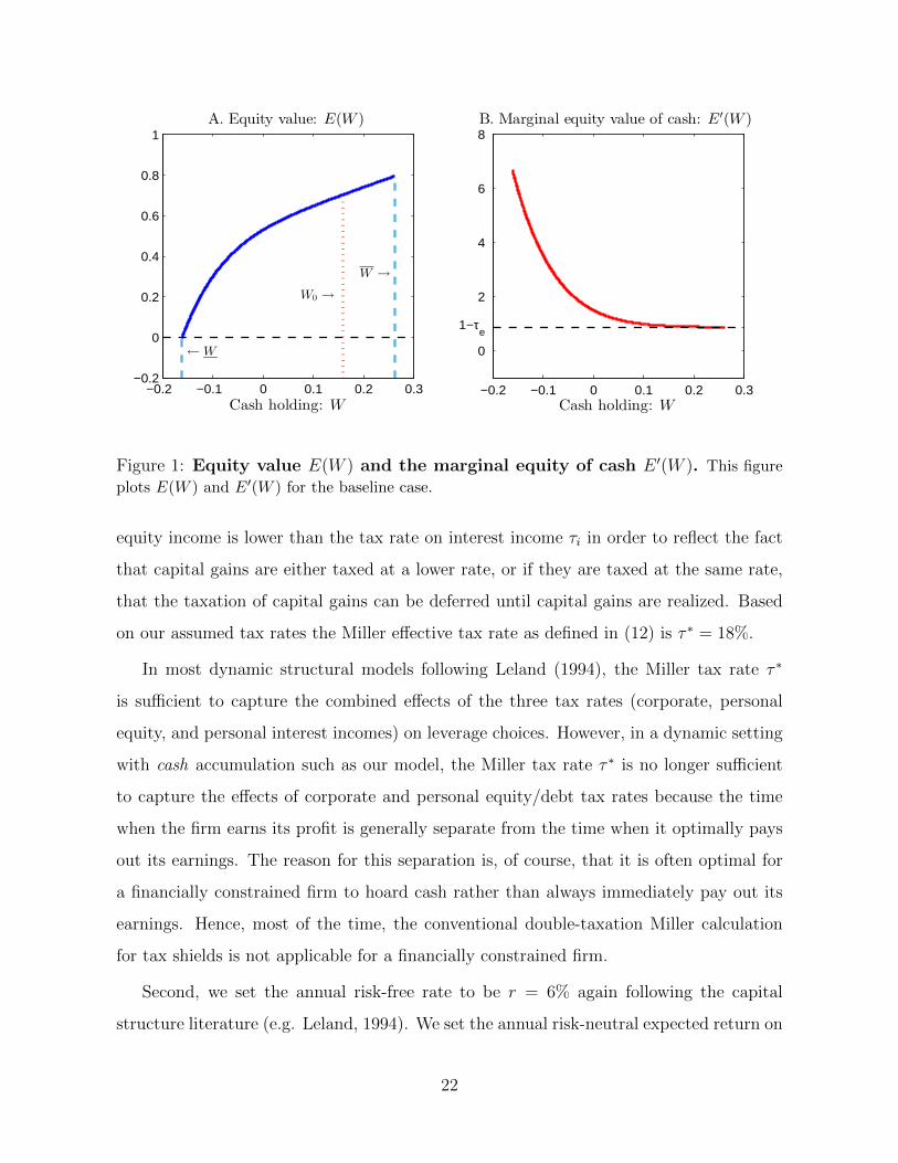
The Ex-Post Value of Equity E(W ). Figure 1 plots the value of equity E(W ) in

Panel A and the marginal equity value of cash E ′(W ) in Panel B in the interior region

[−C,W ]. For our baseline parameter values the optimal LOC commitment is C = 0.16,

the optimal coupon is b = 0.0756, and there is no outside equity stake, a = 0. Moreover,

the optimal start-up cash buffer is W0 = 0.1635 and the optimal payout boundary is

W = 0.2645, as can be seen in Panel A. The entrepreneur obtains an initial equity value

of V0 = 0.7033 under the optimal capital structure.

24

When W reaches the endogenous lower boundary W = −C = −0.16, the firm has run

out of its maximal liquidity supply and is liquidated. At that point equity is worthless,

as liabilities exceed assets. When W hits W = 0.2645, it is optimal for the firm to pay

out any cash in excess of W . Indeed at that point the marginal value of cash inside the

firm for equityholders is just equal to the after-tax value of a marginal payout: E ′(W ) =

(1 − τe) = 0.88, as can be seen in Panel B. In the interior region, equity value E(W )

increases with W with a slope E ′(W ) > (1 − τe), reflecting the value of a higher cash

buffer as insurance against the risk of early liquidation. As can be seen in Panel B, when

the firm is close to running out of cash, the marginal value of one dollar to equity holders

exceeds six dollars.

Remarkably, E(W ) is concave in W even though the firm is levered with risky debt.

As is well known, in a static setting the value of equity for a firm with risky debt on its

books is equivalent to the value of a call option with strike price equal to the face value

of the firm’s debt. It follows from this observation that the value of equity is convex in

the value of the firm’s underlying assets. However, as Panel A reveals, when the firm can

engage in precautionary corporate savings it becomes dynamically risk averse even when

it is highly levered. The reason why the firm is dynamically risk averse is that at any

moment in time its dominant concern is to survive, as its continuation value exceeds the

liquidation value. This is why it is optimal for the firm to start with a relatively large

cash buffer W0 = 0.16 and to secure a large LOC commitment of C = 0.16.

The Ex-Post Value of Debt. Figure 2 plots: 1) the value of debt D(W ) in Panel A;

2) the marginal debt value of cash D′(W ) in Panel B; 3) net debt D(W ) −W in Panel

C; and, 4) the credit spread S(W ) = (b/D(W ) − r) in Panel D, in the interior region

[−C,W ]. A first observation that emerges from Figure 2 is that the market value of debt

D(W ) is increasing and concave in W , and the credit spread is decreasing in W . This is

intuitive, given that the firm is less likely to default when it has a higher cash buffer. This

is also in line with the evidence provided in Acharya, Davydenko and Strebulaev (2012).8

8Acharya, Davydenko and Strebulaev (2012) first run an OLS regression of yield spreads on cash-to-total assets and other variables. They obtain a positive coefficient, suggesting that surprisingly higher

25

A second observation is that the slope D′(W ) is highly sensitive to W . Note that as W

increases towards the endogenous payout boundary W = 0.16, D′(W ) approaches zero,

indicating that debt becomes insensitive to the increase in W .

A third striking observation is that net debt, D(W ) − W , is non-monotonic in W ,

which suggests that net debt is a poor measure of a firm’s credit risk. Analysts commonly

use net debt as a measure of a firm’s credit risk on the logic that the firm could at any

time use its cash hoard to retire some or all of its outstanding debt. As our results

show, information may be lost by netting debt with cash, as the netted number of 1.1 for

example could reflect either a high credit risk (if the firm is drawing down on its LOC) or

a low credit risk if the firm holds a comfortable cash buffer W in excess of 0.1 (see Panel

C).

Finally, Panel D plots the credit spread S(W ) = b/D(W ) − r, which is basically a

decreasing and convex transformation of debt value D(W ) given in Panel A. It decreases

to 0.05% as W approaches the endogenous payout boundary W = 0.16, and when the

firm exhausts its the credit line limit C = 0.16 the credit spread increases beyond 400

basis points. Note that even at the payout boundary, the firm’s debt is not risk free as

there is still a small probability that the firm ends up in liquidation.

The Ex-Post Enterprise Value. Figure 3 plots the enterprise value Q(W ) = V (W )−

W in Panel A, and the marginal enterprise value of cash Q′(W ) in Panel B. Given that

both equity value and debt value are increasing and concave in W , we expect that enter-

prise value Q(W ) is more concave than equity value E(W ). This means that an investor

holding a portfolio of debt and equity in this firm would be more averse to cash-flow risk

than an equity holder. Thus, although equity-holders are dynamically risk-averse, they

are not risk-averse enough to be in a position to optimally control risk from the point of

view of total firm value. This is why, it is optimal in general to include debt covenants

into the term debt contract, that limit equity-holders’ ability to control risk or pay out

cash holdings are associated with higher spreads. However, when they run an instrumental variableregression (using the ratio of intangible-to-total assets as an instrument) they find that the coefficient onthe cash-to-total assets variable is negative.

26

dividends ex post.

Note that the marginal enterprise value Q′(W ) can be negative for values of W that

exceed 0.140. How can marginal enterprise value of cash be negative? This is due to the

fact that paying out excess cash triggers personal equity income tax at 12%. Therefore, at

the payout boundary W = 0.26, Q′(0.26) = −0.12 < 0. Because Q′(W ) can be negative,

we should be somewhat cautious with the economic interpretation of enterprise value

Q(W ) in environments with (personal equity) taxes.

Leverage. We define market leverage, denoted by L(W ), as the ratio between the mar-

ket value of debt, D(W ), and the firm’s market value V (W ),

L(W ) =D(W )

V (W ). (34)

Another common definition of leverage replaces debt value with ‘net debt’ D(W ) −W

and accordingly replaces firm value V (W ) by enterprise value Q(W ). We refer to this

leverage ratio as ‘net leverage’, and denote it by LN(W ),9

LN(W ) =D(W )−WQ(W )

.

Figure 4 plots both leverage L(W ) and net leverage LN(W ) as a function of W in the

interior region. Both measures of leverage are decreasing in W . When the firm runs

out of liquidity, the firm becomes insolvent, the value of equity is zero, E(−C) = 0, so

that leverage takes its maximum value of 100%. At the payout boundary W , market

leverage reaches its minimum value of 45.9%. This may appear to be a high level of

leverage. However, note that for an unconstrained firm, the Miller solution described

above prescribes market leverage of 100%. An important reason why we obtain high

leverage ratios even for a financially constrained firm is that underlying cash-flow risk in

our model is i.i.d.

9Acharya, Almedia, and Campello (2007) argue that cash should not be treated as negative debt.Cash can help financially constrained firms hedge future investment against income shortfalls, so thatconstrained firms would value cash more. Our model provides a precise measure of this distortion.

27

−0.2 −0.15 −0.1 −0.05 0 0.05 0.1 0.15 0.2 0.25 0.30.5

0.6

0.7

0.8

0.9

1

1.1

Leverag

e

Cash holding: W

L(W )L

N (W )

Figure 4: Leverage L(W ) and net leverage LN(W ). This figure plots market leverage

L(W ) and net leverage LN (W ) against liquidity W .

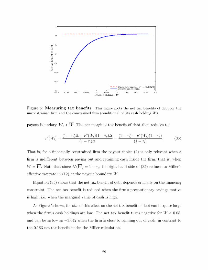
The Tax Advantage of Debt for a Financially Constrained Firm. How does

the net tax benefit of debt for the financially constrained firm compare to that for an

unconstrained firm under the standard Miller (1977) calculation? To address this question

it is helpful to consider how a marginal dollar increment in income generated inside the

firm may be used. A marginal ∆ increment in income can be used in one of the following

ways: (1) paid out to service debt, (2) paid out to equityholders as a dividend, or (3)

retained inside the firm as liquidity reserve. The after-tax interest income to debt holders

is (1 − τi)∆ and the after-tax dividend income to equity holders is (1 − τc)(1 − τe)∆.

Finally, if the amount ∆ is retained, the firm’s cash reserve will increase by (1 − τc)∆,

resulting in an after-tax capital gain of E(Wt + (1 − τc)∆) − E(Wt), or approximately

E ′(Wt)(1− τc)∆ for small ∆.

In the absence of external financing costs there is no need to retain cash. The net tax

benefit of debt is then based on the comparison between choices (1) and (2), which gives

the effective Miller tax rate in (12). In the presence of external financing costs the firm

prefers to retain cash instead of paying it out whenever Wt is away from the endogenous

28

−0.2 −0.15 −0.1 −0.05 0 0.05 0.1 0.15 0.2 0.25 0.3−6

−5

−4

−3

−2

−1

0

1

Net

taxbe

nefitof

debt

Cash holding: W

Unconstrained: τ∗ = 0.1829Constrained firm

Figure 5: Measuring tax benefits. This figure plots the net tax benefits of debt for the

unconstrained firm and the constrained firm (conditional on its cash holding W ).

payout boundary, Wt < W . The net marginal tax benefit of debt then reduces to:

τ ∗(Wt) =(1− τi)∆− E ′(Wt)(1− τc)∆

(1− τi)∆=

(1− τi)− E ′(Wt)(1− τc)(1− τi)

. (35)

That is, for a financially constrained firm the payout choice (2) is only relevant when a

firm is indifferent between paying out and retaining cash inside the firm; that is, when

W = W . Note that since E ′(W ) = 1− τe, the right-hand side of (35) reduces to Miller’s

effective tax rate in (12) at the payout boundary W .

Equation (35) shows that the net tax benefit of debt depends crucially on the financing

constraint. The net tax benefit is reduced when the firm’s precautionary savings motive

is high, i.e. when the marginal value of cash is high.

As Figure 5 shows, the size of this effect on the net tax benefit of debt can be quite large

when the firm’s cash holdings are low. The net tax benefit turns negative for W < 0.05,

and can be as low as −3.642 when the firm is close to running out of cash, in contrast to

the 0.183 net tax benefit under the Miller calculation.

29

6 Comparative Statics

The solution for our baseline parameter values illustrated above shows that a financially

constrained firm will only exploit the tax advantage of debt to a very limited extent. For

example, close to the endogenous payout boundary W , a financially constrained firm’s

market leverage L(W ) is less than half the optimal market leverage for an unconstrained

firm under the classical dynamic tradeoff solution. But apart from a lower leverage, does

the optimal capital structure of a financially constrained firm also respond to changes

in tax rates or underlying cash-flow characteristics differently from the classical dynamic

tradeoff solution? This is the general question we pursue in this section.

Unlike for the classical dynamic tradeoff solution, a financially constrained firm has

two margins along which it can respond to, say, a change in tax policy: it can change its

debt and it can change its cash policy. In contrast, under the classical dynamic tradeoff

solution for an unconstrained firm, there is only one margin of adjustment, the firm’s level

of debt. Thus when the effective tax benefit of debt τ ∗ increases reliance on debt financing

increases. Similarly, when profitability µ increases, the coupon on perpetual debt b also

increases. How robust are these predictions to the introduction of financial constraints?

We address this question, by first exploring how a financially constrained firm responds

to changes in tax policy and then considering how the firm changes its financial policy in

response to changes in profitability or earnings volatility.

6.1 Corporate Financial Policy and Taxation

In Table 2, we report the financially constrained firm’s optimal financial policy, market

value and leverage under three different tax policy scenarios. In the first scenario we lower

the corporate tax rate from τc = 0.35 to τc = 0.25 keeping other parameters the same. The

effects of this change on corporate financial policy are reported in the second row of Table 2

and plotted in Figure 6. A cut in the corporate tax rate τc from 35% to 25% substantially

reduces the Miller’s effective tax rate τ ∗ from τ ∗ = 0.183 to τ ∗ = 0.057. Under the

classical dynamic tradeoff solution, one would expect such a decline to significantly lower

30

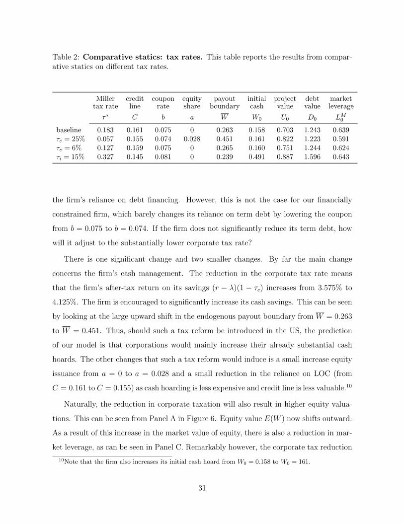
Table 2: Comparative statics: tax rates. This table reports the results from compar-ative statics on different tax rates.

Miller credit coupon equity payout initial project debt markettax rate line rate share boundary cash value value leverage

τ∗ C b a W W0 U0 D0 LM0

baseline 0.183 0.161 0.075 0 0.263 0.158 0.703 1.243 0.639τc = 25% 0.057 0.155 0.074 0.028 0.451 0.161 0.822 1.223 0.591τe = 6% 0.127 0.159 0.075 0 0.265 0.160 0.751 1.244 0.624τi = 15% 0.327 0.145 0.081 0 0.239 0.491 0.887 1.596 0.643

the firm’s reliance on debt financing. However, this is not the case for our financially

constrained firm, which barely changes its reliance on term debt by lowering the coupon

from b = 0.075 to b = 0.074. If the firm does not significantly reduce its term debt, how

will it adjust to the substantially lower corporate tax rate?

There is one significant change and two smaller changes. By far the main change

concerns the firm’s cash management. The reduction in the corporate tax rate means

that the firm’s after-tax return on its savings (r − λ)(1 − τc) increases from 3.575% to

4.125%. The firm is encouraged to significantly increase its cash savings. This can be seen

by looking at the large upward shift in the endogenous payout boundary from W = 0.263

to W = 0.451. Thus, should such a tax reform be introduced in the US, the prediction

of our model is that corporations would mainly increase their already substantial cash

hoards. The other changes that such a tax reform would induce is a small increase equity

issuance from a = 0 to a = 0.028 and a small reduction in the reliance on LOC (from

C = 0.161 to C = 0.155) as cash hoarding is less expensive and credit line is less valuable.10

Naturally, the reduction in corporate taxation will also result in higher equity valua-

tions. This can be seen from Panel A in Figure 6. Equity value E(W ) now shifts outward.

As a result of this increase in the market value of equity, there is also a reduction in mar-

ket leverage, as can be seen in Panel C. Remarkably however, the corporate tax reduction

10Note that the firm also increases its initial cash hoard from W0 = 0.158 to W0 = 161.

31

−0.2 0 0.2 0.40

0.2

0.4

0.6

0.8

1

1.2

W0(τc = 35%) →

W0(τc = 25%) →

A. Equity value: E(W )

−0.2 0 0.2 0.40.7

0.8

0.9

1

1.1

1.2

1.3

1.4B. Debt value: D(W )

−0.2 0 0.2 0.40.5

0.6

0.7

0.8

0.9

1

1.1C. Leverage: L(W )

Cash holding: W−0.2 0 0.2 0.40

100

200

300

400

500D. Credit spread: S(W )

Cash holding: W

τc = 35%τc = 25%

Figure 6: Comparative statics with respect to corporate income tax rate τc.

neither significantly affects the market value of debt nor the credit spread, as can be seen

in Panels B and D respectively.

In the second scenario, we lower the personal tax rate on equity income, τe, from 0.12

to 0.06, a 50% drop in the tax rate. The effects of this change are reported in the third row

of Table 2 and plotted in Figure 7. This change in tax rate τe reduces Miller’s effective tax

benefit of debt τ ∗, which declines from τ ∗ = 0.183 to τ ∗ = 0.127, but the firm’s corporate

financial policy remains essentially unchanged. As can be seen in Figure 7, the reduction

in taxation of equity income results in somewhat higher equity valuations (and a slightly

lower leverage), but otherwise the value of debt and the debt spread remains unchanged.

In the third scenario, we lower the personal tax rate on interest income, τi, from 0.30

to 0.15, again a 50% drop in the personal tax rate. The effects of this change are reported

in the fourth row of Table 2 and plotted in Figure 8. The cut in τi considerably increases

the Miller tax rate, almost doubling τ ∗ from 0.183 to 0.327. This increase in τ ∗ results in a

32

−0.2 −0.1 0 0.1 0.2 0.30

0.2

0.4

0.6

0.8

1

W0(τe = 12%) →

W0(τe = 6%) →

A. Equity value: E(W )

−0.2 −0.1 0 0.1 0.2 0.30.7

0.8

0.9

1

1.1

1.2

1.3

1.4B. Debt value: D(W )

−0.2 −0.1 0 0.1 0.2 0.30.5

0.6

0.7

0.8

0.9

1

1.1C. Leverage: L(W )

Cash holding: W−0.2 −0.1 0 0.1 0.2 0.30

100

200

300

400

500D. Credit spread: S(W )

Cash holding: W

τe = 12%τe = 6%

Figure 7: Comparative statics with respect to personal equity income tax rateτe

significant increase in debt, with the firm raising the coupon from b = 0.075 to b = 0.081.

This increase in the coupon combined with the reduction in τi produces a jump in the

value of outstanding term debt D(W ), as can be seen seen from Panel A in Figure 8. The

firm is then able to raise substantially more cash at time 0 than it wants for precautionary

reasons, with W0 = 0.491 exceeding the payout boundary W = 0.239. This means that

the firm responds to the sharp increase in the effective tax benefit of debt τ ∗ by issuing

so much debt that it can pay out some of the debt proceeds (W0 −W ) immediately to

the entrepreneur.

Interestingly, the other significant change in corporate financial policy is an overall

reduction in the cash buffer the firm chooses to retain, with both a reduction in the LOC

commitment C from 0.161 to 0.145 and a downward shift in the payout boundary W from

0.263 to 0.239. The reason is that, with a higher debt burden the ex-post value of equity

E(W ) (plotted in Panel A of Figure 8) is now lower, so that equityholders–who determine

33

−0.2 0 0.2 0.40

0.2

0.4

0.6

0.8

1

W0(τi = 30%) →

W0(τi = 15%) →

A. Equity value: E(W )

−0.2 −0.1 0 0.1 0.2 0.30.7

0.9

1.1

1.3

1.5

1.7B. Debt value: D(W )

−0.2 −0.1 0 0.1 0.2 0.30.5

0.6

0.7

0.8

0.9

1

1.1C. Leverage: L(W )

Cash holding: W−0.2 −0.1 0 0.1 0.2 0.30

100

200

300

400

500

600D. Credit spread: S(W )

Cash holding: W

τi = 30%τi = 15%

Figure 8: Comparative statics with respect to personal interest income tax rateτi

the firm’s optimal cash policy–are now less concerned to ensure the continuation of the

firm and more interested in getting higher cash payouts. Thus, although equityholders

are dynamically risk averse, from the point of view of maximizing total firm value they

are in effect willing to hoard less cash to be able to get a somewhat higher short-term

payout. Due to the higher coupon and the lower cash buffer, market leverage is higher (as

is seen in Panel C of Figure 8) and the credit spread is also higher (as shown in Panel D of

Figure 8). Overall, the effects of this change in tax policy for financially constrained firms

is closest to the predictions from the classical dynamic tradeoff solution for unconstrained

firms: the increase in τ ∗ results in higher debt financing, higher market leverage, higher

spreads, and a higher probability of default.

34

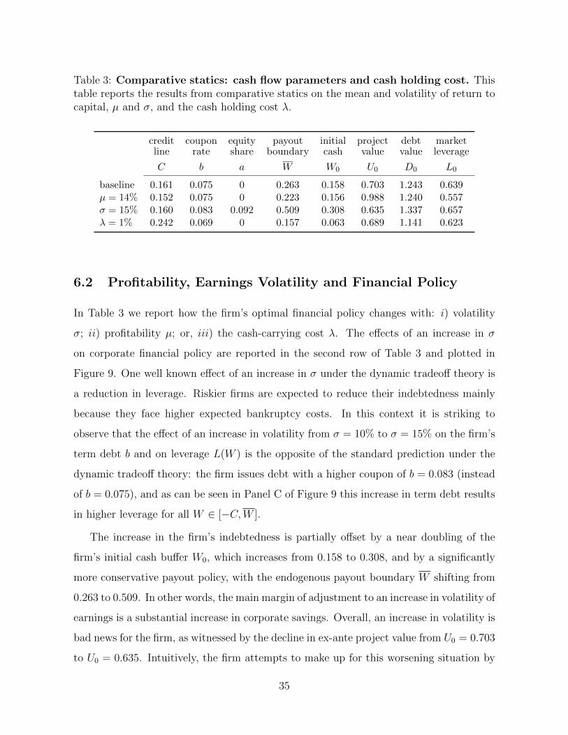
Table 3: Comparative statics: cash flow parameters and cash holding cost. Thistable reports the results from comparative statics on the mean and volatility of return tocapital, µ and σ, and the cash holding cost λ.

credit coupon equity payout initial project debt marketline rate share boundary cash value value leverage

C b a W W0 U0 D0 L0

baseline 0.161 0.075 0 0.263 0.158 0.703 1.243 0.639µ = 14% 0.152 0.075 0 0.223 0.156 0.988 1.240 0.557σ = 15% 0.160 0.083 0.092 0.509 0.308 0.635 1.337 0.657λ = 1% 0.242 0.069 0 0.157 0.063 0.689 1.141 0.623

6.2 Profitability, Earnings Volatility and Financial Policy

In Table 3 we report how the firm’s optimal financial policy changes with: i) volatility

σ; ii) profitability µ; or, iii) the cash-carrying cost λ. The effects of an increase in σ

on corporate financial policy are reported in the second row of Table 3 and plotted in

Figure 9. One well known effect of an increase in σ under the dynamic tradeoff theory is

a reduction in leverage. Riskier firms are expected to reduce their indebtedness mainly

because they face higher expected bankruptcy costs. In this context it is striking to

observe that the effect of an increase in volatility from σ = 10% to σ = 15% on the firm’s

term debt b and on leverage L(W ) is the opposite of the standard prediction under the

dynamic tradeoff theory: the firm issues debt with a higher coupon of b = 0.083 (instead

of b = 0.075), and as can be seen in Panel C of Figure 9 this increase in term debt results

in higher leverage for all W ∈ [−C,W ].

The increase in the firm’s indebtedness is partially offset by a near doubling of the

firm’s initial cash buffer W0, which increases from 0.158 to 0.308, and by a significantly

more conservative payout policy, with the endogenous payout boundary W shifting from

0.263 to 0.509. In other words, the main margin of adjustment to an increase in volatility of

earnings is a substantial increase in corporate savings. Overall, an increase in volatility is

bad news for the firm, as witnessed by the decline in ex-ante project value from U0 = 0.703

to U0 = 0.635. Intuitively, the firm attempts to make up for this worsening situation by

35

−0.2 0 0.2 0.4 0.60

0.2

0.4

0.6

0.8

1

W0(σ = 10%) →

W0(σ = 15%) →

A. Equity value: E(W )

−0.2 0 0.2 0.4 0.60.7

0.8

0.9

1

1.1

1.2

1.3

1.4B. Debt value: D(W )

−0.2 0 0.2 0.4 0.60.5

0.6

0.7

0.8

0.9

1

1.1C. Leverage: L(W )

Cash holding: W−0.2 0 0.2 0.4 0.60

100

200

300

400

500

600D. Credit spread: S(W )

Cash holding: W

σ = 10%σ = 15%

Figure 9: Comparative statics with respect to earnings volatility σ

holding more cash to reduce the probability of an early liquidation and by exploiting the

tax-shield benefits of debt more aggressively. It is worth noting finally that the increase in

volatility also induces the firm to issue outside equity (an increase from a = 0 to a = 0.092)

to ensure that the firm starts out with a sufficient cash buffer W0. In sum, the main lesson

emerging from this comparative statics exercise is that the observation of higher debt and

leverage for riskier firms is not necessarily a violation of the tradeoff theory. It points to

the importance of incorporating into the standard model a precautionary savings motive.

The effects of an increase in profitability µ on corporate financial policy are reported

in the third row of Table 3 and plotted in Figure 10. Under the classical dynamic tradeoff

solution, an increase in profitability µ from 12% to 14% will result in a proportional

increase in the coupon b. Simply put, higher profits require a higher tax shield, which

is obtained by committing to higher interest payments, b. Remarkably, this seemingly

obvious prediction is not borne out for a financially constrained firm. As can be seen in

36

−0.2 −0.1 0 0.1 0.2 0.30

0.2

0.4

0.6

0.8

1

1.2

W0(µ = 12%) →

W0(µ = 14%) →

A. Equity value: E(W )

−0.2 −0.1 0 0.1 0.2 0.30.7

0.8

0.9

1

1.1

1.2

1.3

1.4B. Debt value: D(W )

−0.2 −0.1 0 0.1 0.2 0.30.5

0.6

0.7

0.8

0.9

1

1.1C. Leverage: L(W )

Cash holding: W−0.2 −0.1 0 0.1 0.2 0.30

100

200

300

400

500D. Credit spread: S(W )

Cash holding: W

µ = 12%µ = 14%

Figure 10: Comparative statics with respect to profitability µ

Table 3, the firm keeps its coupon unchanged at b = 0.75 and mainly adjusts its LOC

commitment from C = 0.161 to C = 0.152, and its payout boundary W , which shifts

down from 0.263 to 0.223. In other words, the firm keeps long-term debt unchanged, but

reduces its retained earnings, as it can replenish its cash stock more quickly thanks to a

higher profitability µ. As a result of this policy response, firm equity value increases (see

Panel A in Figure 10) and leverage decreases (Panel C in Figure 10), with no visible effect

on debt value D(W ) or the debt spread (Panels B and D in Figure 10). Once again, the

main margin of adjustment is the firm’s cash policy and not its debt policy. It has often

been pointed out that in practice firm leverage appears to be unresponsive to changes in

profitability, which is generally interpreted as a violation of the static tradeoff theory (see

e.g. Rajan and Zingales, 1995). A common explanation given for this violation is that

more profitable firms have more growth options and therefore face greater debt-overhang

costs. In our model the firm does not have any growth options, yet its debt is unresponsive

37

−0.2 −0.1 0 0.1 0.2 0.30

0.2

0.4

0.6

0.8

W0(λ = 0.5%) →

W0(λ = 1%) →

A. Equity value: E(W )

−0.2 −0.1 0 0.1 0.2 0.3

0.7

0.8

0.9

1

1.1

1.2

1.3

1.4B. Debt value: D(W )

−0.2 −0.1 0 0.1 0.2 0.30.5

0.6

0.7

0.8

0.9

1

1.1C. Leverage: L(W )

Cash holding: W−0.2 −0.1 0 0.1 0.2 0.3

0

100

200

300

400

500D. Credit spread: S(W )

Cash holding: W

λ = 0.5%λ = 1%

Figure 11: Comparative statics with respect to cash-carrying cost λ

to changes in profitability. The reason is that the firm adjusts its cash policy rather than

its debt. Thus, if one takes into account the reality that financially constrained firms have

precautionary savings motive and also seek to reduce their tax burdens, their financial

policy may no longer be so puzzling.

Finally, the effects of an increase in the cash-carrying cost λ on corporate financial

policy are reported in the fourth row of Table 3 and plotted in Figure 11. The main effect

of an increase in the cash-carrying cost λ from 0.5% to 1% is to substantially reduce the

firm’s retained earnings. The initial stock of cash drops from W0 = 0.158 to W0 = 0.063,

and the endogenous payout boundary W shifts down from 0.263 to 0.157. The firm

makes up for its lower cash reserves by taking out a substantially larger LOC, with the

commitment C increasing from 0.161 to 0.242. The firm also reduces its term debt from

b = 0.075 to b = 0.069 in response to the increase in its debt servicing costs. The overall

effect of this policy response is to increase the value of equity (as shown in Panel A in

38

Figure 11), decrease leverage (shown in Panel C of Figure 11) and the value of debt D(W )

(shown in Panel B of Figure 11), and decrease the debt spread (Panel D of Figure 11).

7 Covenants

Bond covenants that protect bondholders in situations where a conflict arises between

equityholders and debtholders are ubiquitous. In our model such a conflict can arise over

payout policies, as the payout boundary is determined to maximize equity value E(W )

and not total firm value V (W ). How do the firm’s financial policies change when we

introduce debt covenants into the bond contract? This is the question we address in this

section.

There are many different forms of bond covenants, ranging from interest service cov-

erage ratios to restrictions on capital expenditures and new debt issuance. Leland (1994)

considers both covenants on the firm’s bankruptcy decision and its cash payouts. Specif-

ically, he imposes a solvency covenant, whereby the firm is forced into bankruptcy as

soon as the value of its assets is equal to the principal value of the debt: VB = P . As

he acknowledges: “such covenants are not common in long-term bond contracts”, and in

his model there is no benefit for the firm in introducing such a covenant, since total firm

value is lower when such covenants are in place. Leland (1994) also considers covenants

that regulate “cash payouts”, which are modeled as a reduction in the rate of return on

the firm’s asset (the expected return on V is (r− d) instead of r). He considers payouts d

that cover both dividend payments and a fraction of the coupon payment C, and shows

that any such payouts d ≥ 0 lower the value of the firm, as they increase the incidence of

costly bankruptcy. The modeling of cash payouts in Leland (1994) is inevitably contrived

given that neither cash-flows nor retained earnings are explicitly modeled.

In contrast, in our framework covenants on cash payouts can be explicitly modeled.

Specifically, an optimal covenant on cash payouts in our model is a payout boundary W 0

that is chosen to maximize total ex-post firm value V (W ) = E(W ) + D(W ) instead of

just ex-post equity value E(W ). Thus, an optimal payout boundary W∗

must satisfy the

39

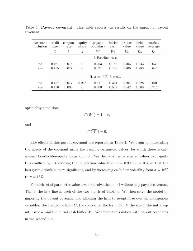
Table 4: Payout covenant. This table reports the results on the impact of payoutcovenant.

covenant credit coupon equity payout initial project debt marketinclusion line rate share boundary cash value value leverage

C b a W W0 U0 D0 L0

I. Baseline case

no 0.161 0.075 0 0.263 0.158 0.703 1.243 0.639yes 0.155 0.077 0 0.321 0.196 0.706 1.283 0.645

II. σ = 15%, L = 0.3

no 0.157 0.077 0.258 0.511 0.341 0.604 1.228 0.601yes 0.156 0.098 0 0.800 0.502 0.642 1.608 0.715

optimality conditions

V ′(W∗) = 1− τe

and

V ′′(W∗) = 0.

The effects of this payout covenant are reported in Table 4. We begin by illustrating

the effects of the covenant using the baseline parameter values, for which there is only

a small bondholder-equityholder conflict. We then change parameter values to magnify

this conflict, by: i) lowering the liquidation value from L = 0.9 to L = 0.3, so that the

loss given default is more significant, and by increasing cash-flow volatility from σ = 10%

to σ = 15%.

For each set of parameter values, we first solve the model without any payout covenant.

This is the first line in each of the two panels of Table 4. We then solve the model by

imposing the payout covenant and allowing the firm to re-optimize over all endogenous

variables: the credit-line limit C, the coupon on the term debt b, the size of the initial eq-

uity issue a, and the initial cash buffer W0. We report the solution with payout covenants

in the second line.

40

The effects of the introduction of the covenants can be seen by comparing the results

in the two lines. For the baseline parameter values we find that:

1. The introduction of a payout covenant shifts the payout boundary from W = 0.263

to W∗

= 0.321, so that the firm holds a larger buffer of internal funds that can be

used to service its term debt;

2. As a result, the firm can afford to issue more term debt and its coupon increases

from b = 0.075 to b = 0.077; this results in a higher debt value (D0 = 1.283 instead

of D0 = 1.243), and higher leverage (L0 = 0.645 instead of L0 = 0.639);

3. The higher debt issuance also results in a higher initial cash buffer (W0 = 0.196

instead of W0 = 0.158) and a slightly higher project value (U0 = 0.706 versus

U0 = 0.703).

While the quantitative effects are small (due to the muted conflict under the baseline

parameter values), some of the qualitative effects are striking, such as the higher optimal

leverage when payout covenants are included.

These effects are confirmed and magnified when we look at the solutions under the

new parameter values (σ = 15% and L = 0.3). Thus we find that:

1. The introduction of a payout covenant now markedly shifts the payout boundary

from W = 0.511 to W∗

= 0.800;

2. As a result, the firm markedly reduces its reliance on outside equity financing,

lowering the fraction of equity it issues to outsiders from a = 0.258 to a = 0.109;

3. The firm also issues more term debt, as its coupon increases from b = 0.077 to

b = 0.098. The combination of lower equity issuance and higher debt results in

substantially higher leverage (L0 = 0.715 instead of L0 = 0.601);

4. Finally, the initial cash buffer is also substantially higher (W0 = 0.502 instead

of W0 = 0.341) and project value is also significantly affected by the covenant

(U0 = 0.642 instead of U0 = 0.604).

41

−0.2 0 0.2 0.4 0.6 0.80

0.5

1

1.5

2

2.5

3A. Firm value: V (W )

−0.2 0 0.2 0.4 0.6 0.80

0.2

0.4

0.6

0.8

1B. Equity value: E(W )

−0.2 0 0.2 0.4 0.6 0.80

0.5

1

1.5

2C. Debt value: D(W )

Cash holding: W−0.2 0 0.2 0.4 0.6 0.80

1000

2000

3000

4000

5000

6000

7000D. Credit spread (bps)

Cash holding: W

with covenantwithout covenant

Figure 12: Impact of debt covenant.

The effects of the payout covenant can be seen in greater detail in Figure 12. Panels A

and C reveal that most of the gain from the covenant arises for values of W ∈ [W,W∗]. At

lower values of W neither V (W ) nor D(W ) are much affected. Moreover, by comparing

Panels B and D we can observe that the significant increase in debt value D(W ) from the

covenant comes only at the expense of a small reduction in equity value E(W ). Finally,

Panel D reveals that the covenant has virtually no effect on the credit spread. In sum, the

most significant effect of the covenant is to substantially increase debt value and optimal

leverage.

42

8 Recurrent external equity financing

When the project’s expected productivity µ is high and the fixed cost of external financing

Φ is low the firm will want to raise fresh external funds rather than force the project into

early liquidation when it runs out of cash. We now analyze this situation by letting the

firm raise new funds whenever it runs out of cash. For simplicity, we only let the firm

issue equity in this case. Moreover, we make the further simplifying assumption that the

new equity is allocated to existing shareholders in proportion to their ownership, so that

the entrepreneur’s initial ownership stake (1− a) remains unchanged.

Let M > 0 denote the total amount of liquidity after the new equity issue, which we

we refer to as the liquidity “return” point after equity issue. This amount is chosen to

maximize the total value of equity E(W ). Given that equity value is continuous before

and after the seasoned equity offering (SEO) the following boundary condition for E(W )

must hold at at the boundary |W | = C:

E(−C) = E(M)− Φ− M + C

1− γE. (36)

Note that an equity issue only occurs when the firm exhausts its credit line, as the firm

has to pay a commitment fee to have a credit line even for the unused portion. Hence,

the firm will only commit to a credit line that it may eventually want to tap under some

circumstances. As M is the post-issue amount of liquidity, the total (net) amount of issue

is then M+C, which can be either positive or negative. If 0 < M < −C, the firm remains

in the credit region after equity issue. If M ≥ −C, the firm enters into the cash region

after equity issue. The right-hand side represents the post-SEO equity value minus both

the fixed and the proportional costs of equity issuance. Second, since the “return” point

M is optimally chosen, the marginal value of the last dollar raised must be equal to the

cost of the fund, 1/(1− γE). This gives the following smooth-pasting boundary condition

at M :

E ′(M) =1

1− γE. (37)

43

Table 5: Comparative statics: Refinancing case. This table reports the results fromcomparative statics on the financing cost parameters in the refinancing case.

(Φ, γE , γD) b C a U0 D0 E(−C) W0 W M

(1.0, 6.0, 6.0) 0.067 0.148 0 0.733 1.124 0.531 0.047 0.111 -0.082(0.1, 6.0, 6.0) 0.066 0.142 0 0.746 1.098 0.579 0.031 0.078 -0.117(1.0, 4.0, 6.0) 0.067 0.148 0 0.733 1.120 0.538 0.043 0.108 -0.078(1.0, 6.0, 4.0) 0.095 0.124 0 0.756 1.582 0.161 0.509 0.205 -0.037(0.1, 6.0, 4.0) 0.102 0.117 0 0.770 1.702 0.089 0.633 0.189 -0.082(0.0, 6.0, 6.0) 0.066 0.140 0 0.749 1.095 0.591 0.029 0.060 –

The firm’s equityholders will obviously only choose the refinancing option if

E(−C) = E(M∗)− Φ− M∗ + C

1− γE≥ 0 (38)

where M∗ satisfies the optimality condition given in (37). Given that E(M∗) is a de-

creasing function of the coupon payment b, condition (38) puts an upper bound on how

much term debt the firm can issue at time 0, while credibly committing to permanently

servicing this debt. Any coupon below this upper bound will always be serviced, as the

firm will always prefer to raise new equity when it runs out of cash. Thus, any such term

debt will be safe and will be valued at D = b/r.

Table 5 describes the firm’s optimal financial policy and market value under six dif-

ferent settings for external financing costs. The first row is the baseline case for which

Φ = 1% and γE = γD = 6%. The first major result emerging from this analysis is that in

the baseline case as well as all other five cases the constraint E(−C) ≥ 0 is not binding.

This implies that the optimal tradeoff between tax benefits of debt and servicing costs

is obtained for a value of the coupon b that does not exhaust all the tax shield benefits

that are potentially available to the firm. A major critique of the tradeoff theory is that

it must be false since: “If the theory is right, a value-maximizing firm should never pass

up interest tax shields when the probability of financial distress is remotely low.” [Myers,

2001] But, as our analysis illustrates this critique only applies to financially unconstrained

44

−0.2 −0.1 0 0.1 0.20.5

0.55

0.6

0.65

0.7

0.75

0.8

W0(Φ = 1.0%) →

W0(Φ = 0.1%) →

A. Equity value: E(W )

−0.2 −0.1 0 0.1 0.20.8

0.9

1

1.1

1.2

1.3

1.4

1.5B. Marginal equity value of cash: E′(W )

−0.2 −0.1 0 0.1 0.20.5

0.55

0.6

0.65

0.7

0.75

0.8

W0(γE = 6%) →

W0(γE = 4%) →

Cash holding: W

C. Equity value: E(W )

−0.2 −0.1 0 0.1 0.20.8

0.9

1

1.1

1.2

1.3

1.4

1.5

Cash holding: W

D. Marginal equity value of cash: E′(W )

Φ = 1.0%Φ = 0.1%

γE = 6%γE = 4%

Figure 13: Comparative statics for the refinancing case: Φ and γE

firms. When firms face external financing costs, the optimal tradeoff between tax shield

benefits of debt and servicing costs may well be obtained with safe debt, for which there

is no credit risk whatsoever.

The five cases other than the baseline case all involve lower financing costs and illus-

trate the effects of respectively lowering: i) the fixed cost to Φ = 0.1% in the second row

and to Φ = 0.0% in the last row (keeping the variable costs γE and γD unchanged); ii)

the variable cost of equity to γE = 4% in the third row (keeping the fixed cost Φ and the

variable cost γD unchanged); and iii) the variable cost of debt to γD = 4% in the fourth

row (keeping the fixed cost Φ and the variable cost γE unchanged), and the fifth row,

where the fixed cost is also lowered to Φ = 0.1%. The point of these different scenarios is

to show how the financially constrained firm’s debt policy varies with external financing

costs.

45

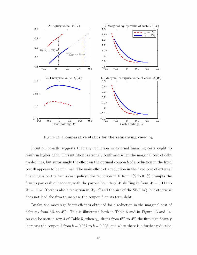
−0.2 0 0.2 0.4 0.60.1

0.3

0.5

0.7

0.9

W0(γD = 6%) →

W0(γD = 4%) →

A. Equity value: E(W )

−0.2 −0.1 0 0.1 0.2 0.30.8

0.9

1

1.1

1.2

1.3

1.4

1.5B. Marginal equity value of cash: E′(W )

−0.2 −0.1 0 0.1 0.2 0.31.75

1.8

1.85

1.9C. Enterprise value: Q(W )

Cash holding: W−0.2 −0.1 0 0.1 0.2 0.3

−0.2

−0.1

0

0.1

0.2

0.3

0.4

0.5D. Marginal enterprise value of cash: Q′(W )

Cash holding: W

γD = 6%γD = 4%

Figure 14: Comparative statics for the refinancing case: γD

Intuition broadly suggests that any reduction in external financing costs ought to

result in higher debt. This intuition is strongly confirmed when the marginal cost of debt

γD declines, but surprisingly the effect on the optimal coupon b of a reduction in the fixed

cost Φ appears to be minimal. The main effect of a reduction in the fixed cost of external

financing is on the firm’s cash policy: the reduction in Φ from 1% to 0.1% prompts the

firm to pay cash out sooner, with the payout boundary W shifting in from W = 0.111 to

W = 0.078 (there is also a reduction in W0, C and the size of the SEO M), but otherwise

does not lead the firm to increase the coupon b on its term debt.

By far, the most significant effect is obtained for a reduction in the marginal cost of

debt γD from 6% to 4%. This is illustrated both in Table 5 and in Figure 13 and 14.

As can be seen in row 4 of Table 5, when γD drops from 6% to 4% the firm significantly

increases the coupon b from b = 0.067 to b = 0.095, and when there is a further reduction

46

in the fixed cost Φ to 0.1% then the coupon only marginally increases to b = 0.102 (see

row 5). Panels A and B in Figure 13, which respectively plot the firm’s Equity value

E(W ), and the marginal value of cash E ′(W ), show that the main effect of a drop in

the fixed cost Φ is an increase in equity value and a reduction in the marginal value of

cash. Similarly, Panels C and D in figure 13 show that a reduction in the marginal cost

of equity γE from 6% to 4% has virtually no effect.

In contrast, Panels A and C in figure 14 display the substantial effect of a reduction

in the marginal cost of debt γD from 6% to 4%. This produces a significant increase in

enterprise value (Panel C) and a reduction in equity value (Panel A). The firm basically

takes advantage of the reduction in debt financing costs to raise a substantial amount of

funds W0 = 0.509 at time 0 and to immediately pay out to the founder the difference

(W0 −W ) = 0.304. As can be seen in Panels B and D, this increase in debt has hardly

any effect on the marginal value of cash, which only increases slightly. Note finally that

the other significant effect of the reduction in γD is to induce the firm to almost fully

exhaust the tax benefits of debt, with a reduction in E(−C) from 0.531 to 0.161. The

further reduction in Φ from 1% to 0.1% brings a supplementary drop to E(−C) = 0.089.

9 Conclusion

Although the tax-advantage of debt has long been recognized as an important consider-

ation for corporate financial policy, the tradeoff theory has had an uncertain standing,

with many empirical studies concluding that it is flat-out rejected by the data. We have

shown that one reason why the tradeoff theory performs poorly empirically is that it only

applies to financially unconstrained firms. In the presence of external financing costs,

firms’ financial policy is more complex and involves both a liability and asset manage-

ment dimension. Thus, when there is a change in tax policy, for example, financially

constrained firms generally have two margins along which they can respond: they can

either adjust their debt policy or their cash policy (or both).

As we have shown, the cash management dimension of corporate financial policy radi-

47

cally modifies the classical tradeoff theory. So much so that the theory for unconstrained

firms provides very misleading predictions for corporate financial policies of constrained

firms. Thus, an important new cost of debt financing for financially constrained firms is

the debt servicing cost : interest payments drain the firm’s valuable precautionary cash

holdings and thus impose higher expected external financing costs on the firm. Interest

payments may help shield earnings from corporate taxation, but they potentially induce

inefficient liquidation or costly external financing. Because liquidity/cash is valuable for a

financially constrained firm, the firm thus has an optimal portfolio choice among external

equity, debt, and liquidity including both cash and a credit line. We show that cash is

not negative debt, and we offer a novel explanation for the “debt conservatism puzzle” by

showing that financially constrained firms choose to limit their debt and interest expenses

in order to preserve their cash holdings.

Another important change introduced by external financing costs is that realized earn-

ings are generally separated in time from payouts to shareholders, implying that the clas-

sical Miller-formula for the net tax benefits of debt no longer holds. We show that the

standard Miller effective tax rate calculation only applies at the payout boundary. In the

cash-hoarding and credit regions, the tax calculation is very different as the firm defers

its payment to shareholders and thus the standard Miller formula does not apply. We

further show that the firm may not even exhaust its risk-free debt capacity because ser-

vicing debt can be expensive. Finally, our model is a valuation model for debt and equity

in the presence of taxes and external financing costs. It shows how the classical adjusted

present value methodology breaks down for financially constrained firms, as it does not

account for the value of cash for both debt and equity.

Two major simplifications of our analysis are: i) that the firm only faces iid cash-

flow shocks, and ii) that there is only one fixed productive asset. These assumptions

mainly help make the analysis very transparent. In future research, we plan to extend our

framework to incorporate both persistent and potentially permanent productivity shocks

and dynamic corporate investment. These extensions will make our model even more

suitable for the study of tax policy changes on corporate investment, corporate savings,

48

and firm valuations. Needless to say, such an analysis would be particularly relevant

given the current fiscal policy debate. We believe that our framework is a natural starting

point to think about these issues at the intersection between public finance and corporate

finance.

49

References

Acharya, V., S. A. Davydenko, and I. A. Strebulaev, 2012, “Cash Holdings and Credit

Risk,” Review of Financial Studies, 25, 3572–3609.

Acharya, V. V., H. Almeida, and M. Campello, 2007, “Is cash negative debt? A hedging

perspective on corporate financial policies,” Journal of Financial Intermediation, 16,

515–554.

Acharya, V. V., H. Almeida, and M. Campello, 2010, “Aggregate Risk and the Choice

between Cash and Lines of Credit,” Working Paper.

Almeida, H., M. Campello, and M. S. Weisbach, 2004, “The cash flow sensitivity of cash,”

Journal of Finance, 59, 1777–1804.

Bates, T. W., K. M. Kahle, and R. M. Stulz, 2009, “Why Do U.S. Firms Hold So Much

More Cash than They Used To?,” Journal of Finance, 64, 1985–2021.

Bolton, P., H. Chen, and N. Wang, 2011, “A Unified Theory of Tobin’s q, Corporate

Investment, Financing, and Risk Management,” Journal of Finance, 66, 1545–1578.

Bolton, P., H. Chen, and N. Wang, 2013, “Market Timing, Investment, and Risk Man-

agement,” Journal of Financial Economics, 109, 40–62.

Collins, J. H., and D. Kemsley, 2000, “Capital Gains and Dividend Taxes in Firm Valua-

tion: Evidence of Triple Taxation,” The Accounting Review, 75, 405–427.

DeAngelo, H., L. DeAngelo, and T. Whited, 2011, “Capital Structure Dynamics and

Transitory Debt,” Journal of Financial Economic, 99, 235–261.

DeAngelo, H., and R. W. Masulis, 1980, “Optimal capital structure under corporate and

personal taxation,” Journal of Financial Economics, 8, 3–29.

Decamps, J., T. Mariotti, J. Rochet, and S. Villeneuve, 2011, “Free Cash Flow, Issuance

Costs, and Stock Prices,” Journal of Finance, 66, 1501–1544.

50

DeMarzo, P. M., and M. J. Fishman, 2007, “Optimal Long-Term Financial Contracting,”

Review of Financial Studies, 20, 2079–2128.

DeMarzo, P. M., and Y. Sannikov, 2006, “Optimal Security Design and Dynamic Capital

Structure in a Continuous-Time Agency Model,” Journal of Finance, 61, 2681–2724.

Duffie, D., and K. Singleton, 1999, “Modeling Term Structures of Defaultable Bonds,”

Review of Financial Studies, 12, 687–720.

Fischer, E. O., R. Heinkel, and J. Zechner, 1989, “Dynamic Capital Structure Choice:

Theory and Tests,” Journal of Finance, 44, 19–40.

Frank, M. Z., R. Singh, and T. Y. Wang, 2010, “Personal Income Taxes and Corporate

Investment,” Working Paper, University of Minnesota.

Goldstein, R., N. Ju, and H. Leland, 2001, “An EBIT-Based Model of Dynamic Capital

Structure,” Journal of Business, 74, 483–512.

Graham, J. R., 2000, “How Big Are the Tax Benefits of Debt?,” Journal of Finance, 55,

1901–1941.

Graham, J. R., 2003, “Taxes and Corporate Finance: A Review,” Review of Financial

Studies, 16, 1075–1129.

Harris, T.-S., and D. Kemsley, 1999, “Dividend Taxation in Firm Valuation : New Evi-

dence,” Journal of Accounting Research, 37, 275–291.

Hennessy, C. A., and T. M. Whited, 2005, “Debt Dynamics,” Journal of Finance, 60,

1129–1165.

Hennessy, C. A., and T. M. Whited, 2007, “How Costly Is External Financing? Evidence

from a Structural Estimation,” Journal of Finance, 62, 1705–1745.

Kim, C.-S., D. C. Mauer, and A. E. Sherman, 1998, “The Determinants of Corporate

Liquidity: Theory and Evidence,” Journal of Financial and Quantitative Analysis, 33,

335–359.

51

Leary, M. T., and M. R. Roberts, 2005, “Do Firms Rebalance Their Capital Structures?,”

Journal of Finance, 60, 2575–2619.

Leland, H., 1994, “Corporate Debt Value, bond covenants, and Optimal Capital Struc-

ture,” Journal of Finance, 49, 1213–1252.

Lemmon, M. L., M. R. Roberts, and J. F. Zender, 2008, “Back to the Beginning: Persis-

tence and the Cross-Section of Corporate Capital Structure,” Journal of Finance, 63,

1575–1608.

Merton, R. C., 1974, “On the Pricing of Corporate Debt: The Risk Structure of Interest

Rates,” Journal of Finance, 29, 449–470.

Miller, M. H., 1977, “Debt and Taxes,” Journal of Finance, 32, 261–275.

Miller, M. H., and M. S. Scholes, 1978, “Dividends and taxes,” Journal of Financial

Economics, 6, 333–364.

Myers, S. C., 1974, “Interactions of Corporate Financing and Investment Decisions-

Implications for Capital Budgeting,” Journal of Finance, 29, 1–25.

Myers, S. C., 1984, “The Capital Structure Puzzle,” Journal of Finance, 39, 574–592.

Myers, S. C., 2001, “Capital Structure,” Journal of Economic Perspectives, 15, 81–102.

Panier, F., F. Perez-Gonzalez, and P. Villanueva, 2012, “Capital Structure and Taxes:

What Happens When You (Also) Subsidize Equity?,” Working Paper, Stanford Uni-

versity.

Riddick, L. A., and T. M. Whited, 2009, “The Corporate Propensity to Save,” Journal

of Finance, 64, 1729–1766.

Ross, S. A., 2005, “Capital Structure and the Cost of Capital,” Journal of Applied Fi-

nance, 15, 5–23.

Strebulaev, I. A., 2007, “Do Tests of Capital Structure Theory Mean What They Say?,”

Journal of Finance, 62, 1747–1787.

52

van Binsbergen, J. H., J. Graham, and J. Yang, 2010, “The Cost of Debt,” Journal of

Finance, 65, 2089–2136.

van Binsbergen, J. H., J. Graham, and J. Yang, 2012, “Optimal Capital Structure,”

Working Paper, Stanford University, Duke University, and Georgetown University.

53