a factor-augmented var analysis of the monetary · pdf filea factor-augmented var analysis of...
TRANSCRIPT

1
A Factor-Augmented VAR Analysis of the Monetary Policy in
China1
Pak-Ho LEUNG, Qing HE and Terence Tai-Leung CHONG
Department of Economics, Chinese University of Hong Kong,
School of Finance, Renmin University of China
Department of Economics, Chinese University of Hong Kong
Abstract:
This paper investigates the effects of monetary policy in China over the past two
decades with a typical emphasis on the post-Asian crisis period and the more recent
currency regime shift. A Factor-Augmented VAR method is used to study the
effectiveness of monetary policy instruments in stabilizing the Chinese economy.
We find that the repo rate, benchmark lending rate and a market-based monetary
stance are mildly effective while the growth rates of total loan and of money supply
are significantly effective. Moreover, the effectiveness of the market-based
monetary policies does not improve under a more flexible exchange rate regime. It
is concluded that the central bank in China still depend on the administrative
instruments in stabilizing domestic inflation, and thereby maintaining
macroeconomic and financial stability.
KEYWORDS: Factor Model, Principal Components, VAR, monetary policy
JEL classification: E3, E4, E5, C3
1 We would like to thank Xinhua Gu, Robin Pope and Keen-Meng Choy as well as participants of
the 2009 ACE International Conference for their helpful comments on the earlier version of this
paper. The financial support from the Key Projects in Philosophy and Social Sciences Research
program of the Ministry of Education of the People’s Republic of China (Grant Number 08JZD0011)
is highly appreciated. All remaining errors are ours. Corresponding Author: Terence Tai-Leung
Chong, Department of Economics, The Chinese University of Hong Kong, Shatin, N.T., Hong Kong.
E-mail: [email protected]. Homepage:
http://www.cuhk.edu.hk/eco/staff/tlchong/tlchong3.htm.
2
1. Introduction
In the post-Asian Crisis period, China has achieved remarkable economic growth
for more than a decade, with an average annual growth rate of about 9 percent.
Meanwhile, the inflation rate, as measured by the GDP deflator or CPI, has
remained moderate2. With the termination of official guidance on banks’ lending
operations in 1998, monetary policy has played an increasing role in the
macroeconomic stabilization in China (Green, 2005). However, the transmission
mechanism of the monetary policy remains unclear. Since 1998, a variety of
monetary policy instruments, such as the base interest rates, open market operation,
the discount rate and reserves requirement, have been adopted by the People’s
Banking of China (PBC) to fine tune the economy. However, as the relationship
between these instruments and real economic activities is unstable over time, it
complicates the ways that monetary policy affects the real economies. More
importantly, with the integration into the global economy, the independence and
effectiveness of China’s monetary policy have been challenged because of the
exchange rate rigidity.3 As a result, there has been an increasing attention on the
effects and mechanisms of the Chinese monetary policy.4
In an attempt to shed light on the transmission channels of monetary policy in China,
we employ a new methodology – the Factor-augmented VAR (FAVAR), to
2 The inflation rate remains below 3 percent in most periods. Several researches have found that
Chinese economy has experienced a substantial moderation (Brandt and Zhu (2002), He et al. (2009),
and Du et al. (2010). 3 Goodfriend and Prasad (2007) reported that the Chinese monetary policy has operated with
difficult constraints. 4 For instance, the global financial crisis of 2007-2009, originated in the American mortgage market,
has vaporized the wealth in the advanced economies. Due to a halt in spending in developed
countries, the export-oriented economy of China in jeopardy. In response, the People’s Bank of
China slashes the lending rate as well as the required reserve ratio to support the financially
distressed industries.

3
investigate the effects of several important monetary policy instruments during the
last decade.5 The FAVAR approach allows us to assess how much of the observed
movements of real economy can be attributed to each policy instruments, separately
and in combination.
While significant efforts have been devoted to investigate the effect of Chinese
monetary policies, most of the previous studies employ only a single policy
instrument to measure monetary policy (Mehrotra, 2007; Dickinson and Liu, 2007;
and Koivu, 2009). Our study complements the literature by making a
comprehensive investigation of different monetary policy instruments in China. By
comparing the role of each instrument, our study gains insight into the transmission
mechanism of the Chinese monetary policy. Secondly, to the best of our knowledge,
this is the first attempt to use a combination of policy instruments in the model
estimation. As China usually implements different market-based policy instruments
at the same time, the use of the factor approach may provide an overall evaluation
of its monetary policy. Finally, most of the previous studies have employed the
Vector Autoregression (VAR) approach, which typically comprises of few
variables. The use of sparse information sets in VAR analysis may produce
inaccurate estimates and impulse response pattern (Sims, 1992; Rudebusch, 1998;
and Bernanke et al., 2005). The Factor VAR model combines the standard VAR
approach with factor analysis, and can provide a proper identification of the
monetary transmission mechanism (Stock and Watson, 1998; Bernanke et al., 2005;
Boivin and Giannoni, 2006).
Our results suggest that the Chinese economy is mainly affected by the growth rate
5 The factor VAR procedure has been widely used on the analysis of U.S. and European monetary
policy.

4
of total loan and M2. Other market policy instruments, such as the repo rate and
benchmark lending rate, are only mildly effective in influencing the real economy.
We also show that the general monetary stance representing the overall effects of
market-based instruments only plays a modest role in curbing inflation.
The rest of the paper is organized as follows. Section 2 gives an overview of the
major monetary policies and the transmission mechanism in China. The method of
Factor-Augmented Vector Autoregression (FAVAR) is introduced in Section 3.
Section 4 dwells on the empirical evidence. Section 5 presents the results and policy
implications. Section 6 concludes.
2. Features of Post-Crisis Chinese monetary policy
The People’s bank of China (PBC) has become the central bank of China since 1983,
while it operates under the control of the State Council. An approach of “direct
lending”, is widely used for implementing monetary policy. Though a number of
reforms have been promulgated in the following years (The People’s bank of China,
2005), the lending pattern had little changes till 1998 (Park and Sehrt, 2001), which
indicates scant changes in the implementation of monetary policy.
As the Chinese economy is exposed to more external economic uncertainties, an
independent and effective monetary policy is increasingly crucial for stabilizing
inflation, employment and economic growth (Goodfriend and Prasad, 2007)6. Along
with the liberation and reform in the banking sector, a series of reforms have been
carried out to enhance the effectiveness of the monetary policy. Ever since the
6 For instance, Lardy (2005) points out that the lack of independence of the PBC may result in
counterproductive monetary policy, which leads to a further delay in liberalizing the capital account.
5
termination of “direct lending” in 1998, a variety of monetary instruments have
been implemented. This section will briefly review some important liberalization
policies and a number of key policy instruments since 1998.
2.1 Liberalization of China’s monetary policy in recent years
The People’s Bank of China (PBC) has a dual legal mandate of “maintaining the
stability of the currency, and thereby promoting economic growth”. However, the
persistent double-digit inflation rate in the first half of 1990s, and the outbreak of
the Asian Financial Crisis in 1997, have cast doubt on prospect of the Chinese
economy. A series of banking and financial reforms, especially the liberalization
policies, have shored up the capacity of China’s monetary policy. In 1996 and 1997,
the upper limits on inter-bank lending rate were abolished, and the bond repo
interest rates were liberalized respectively, implying less administrative control over
the money market. More importantly, the credit quota control was scrapped in 1998
and the central bank is able to conduct its monetary policy through indirect tools.
The PBC further liberalizes the interest rates in order to improve the effectiveness of
monetary policy. Since then, the ceiling of RMB lending rate of financial
institutions has been climbing and finally abolished in 2004 (except for the Urban
Credit Cooperatives and Rural Credit Cooperatives). The floor of deposit rate is also
removed in 2004. The lending rate can move unboundedly from 90 percent of the
benchmark lending rate while the ceiling on deposit rate still prevails. In 2007, the
Shanghai Inter-bank Offered Rate (SHIBOR) was formally launched to shore up the
transmission mechanism of the monetary policy (PBC, 2007).
2.2 Monetary policy instruments and their transmission mechanism

6
Since 1998, the PBC is forced to update its monetary tool box to increase the
effectiveness of policy reaction as a consequence of economic environment change.
Besides the administrative instruments, a reform toward market-based instruments
has also been implemented.7
The following section briefly reviews several
important monetary instruments used by the People’s bank of China.
A. Open Market Operation
Open market operation is a major monetary policy used by the PBC to influence the
money market interest rate and the money supply.8 As the open market operation is
carried out on a repo basis, the repo rate is often used as an indicator of China’s
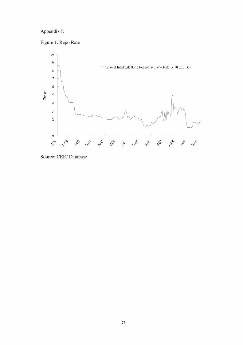
monetary policy9 (Peng et al., 2006). Figure 1 shows that the repo rate declined
from 8.6 percent in 1998 to barely 1 percent in 2005. This rate has been climbing
since 2005 to curb the overheating economy and the escalating inflation. While, the
plunge of repo rate in 2008 provides extensive liquidity for the real economy.
[Insert Figure 1 here]
B. Benchmark lending interest rate
The benchmark interest rate is the reference rate set by the PBC, around which
7 The market-based instruments include open market operation, central bank lending rate, rediscount
rate, required reserve interest rate, excess reserve interest rate, required reserve ratio and benchmark
lending and deposit rate. The administrative instruments are the regulatory change and window
guidance, which is a quantitative manipulation of the bank credit. 8 When the pressure of inflation increases, the PBC can sell central bank bills on a cash or repo basis
in the money market and withdraw money from the commercial banks. With less capital available for
lending, the banks have to raise the lending rate to reflect the real price of capital. The drop in
demand for loan will also lower the consumption, investment and aggregate demand. Consequently,
the pressure of inflation will be relieved. For instance, the issuance of central bank bills in 2008 has
decreased gradually to ensure an ample money supply in the market during the global financial crisis. 9 The 7-day repo rate is often used as a benchmark (Green, 2005)

7
differentiated financial institutions can set their respective commercial lending rates.
As the restrictions of the benchmark interest rate are gradually removed in recent
years, financial institutions are allowed to set their own interest rates according to
the market conditions.
The benchmark interest rate is a key market-based monetary policy to adjust the
broad money supply. Figure 2 shows that the one-year benchmark lending rate has
declined substantially during 1998 and 1999 and remained around two percent until
early 2007. The rate climbs to four percent in 2008 and is slashed again in 2009 due
to the stimulation monetary policy to cope with the Subprime Crisis.
[Insert Figure 2 here]
C. Total Loan
The total amount of credit provided by financial institutions to the economy could
be adjusted by the central bank in various ways. The PBC could employ
market-based instruments, such as the interest rates or required reserve ratio, to
indirectly control the total credit. Though the credit quota is scrapped in 1998,
window guidance10
is still crucial for managing the total amount of credit.
As the window guidance and regulation changes are not quantifiable, one could
shed light on the general monetary direction by tracking the total amount of credit
10
Window guidance is another policy controlling the amount of bank credit and the M2 without
going through the money market and affecting the interest rate. This instrument can also be treated as
a measure to promote certain types of industries. For instance, commercial banks may be instructed
to refrain from lending to industries with high energy consumption, and reinforce the support to the
agricultural sector. Besides, in order to ease the upward pressure of the currency, the PBC has to
keep the interest rates in China significantly lower than those in the United States. The PBC thus
employs the window guidance to control the money supply when other monetary instruments are not
feasible (Lardy, 2005).

8
growth. Figure 3a shows that the growth of financial institution loan has risen from
5 percent in early 2000s to 15 percent in the mid-2000s. The central bank
accelerated the credit creation after 2008, implying a loosening of monetary policy
upon the outbreak of global financial crisis.
[Insert Figure 3a here]
D. Money Supply (M2)
The broad money supply, M2, is the intermediate target of monetary policy of the
PBC and its annual target growth rate is usually announced at the beginning of a
year. The PBC tends to use both market-based and administrative monetary tools to
achieve the target of the M211
. Figure 3 shows that the annual growth rate of money
supply fluctuates around 15 percent between 1998 and 2007. This growth rate
increases substantially to over 25 percent in 2009.
[Insert Figure 4 here]
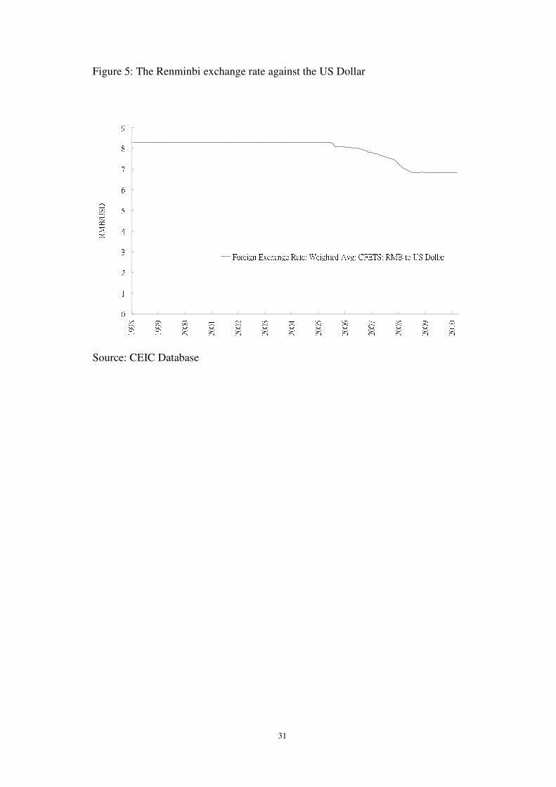
2.3 Exchange Rate reform and the monetary policy
The Chinese currency, the Renminbi, was actually pegged to the US dollar before
July 200512
. The rigidity of exchange rate has limited the capacity of the PBC in
controlling the price level and growth rate via its monetary policy (Prasad et al.,
11
Though M2 and total loan capture the impacts of most policy instruments, their growth targets are
determined separately and their actual growth rates are not necessarily coincide. We consider both
indicators to gauge the general monetary stance in China. 12
Though PBC has announced that the exchange rate was allowed to move around the parity by 0.3
percent, the official rate seldom deviates from the fixed parity.
9
2005). On 21 July 2005, the PBC promulgated reforms in its exchange rate policy
by allowing Renminbi to float in a managed way with reference to a basket of
currencies.13
As shown in Figure 4, the exchange rate between RMB and the US
dollar has climbed from 8.28 in July 2005 to 6.83 February 2010. The reform in the
exchange rate policy has provided the PBC more flexibility in managing the
economy via its monetary policy.
[Insert Figure 4 here]
2.4 Effects of Monetary Policy on the Industrial Production and Inflation
The Chinese economy is characterized by high inflation in the first half of 1990s.
Between 1993 and 1995, there was a huge build-up of price pressure in the domestic
market with the consumer price index rose to 27% in October 1994. The monetary
authorities adopt tightening administrated policies in 1993 and finally brought the
inflation down to a single digit in 1996.
The sustainability of economic growth became a big concern for the Chinese
authorities in the second half of 1990s when the Renminbi remained fixed against
the US dollar, while many Asian countries have depreciated their currencies. Figure
6 shows that China has lost its export competitiveness as the growth of industrial
production has been slowing down since the mid 1990s14
. The consumer price index
(Figure 5) fell from its peak in 1994 to nearly zero in 1998. Given the relatively low
13
The intra-day variation of the Renminbi exchange rate against the US dollar was within 0.3%.
This band was widened to 0.5% in May 2007. 14
The average growth rate between 1994 and 1996 is 17.5, while it is a merely 10.9 percent between
1997 and 1999. Such a low rate of industrial growth is partly due to the Asian Financial Crisis in
1997.

10
inflation rate, the PBC was able to loosen its monetary policy to stimulate the
economy. From 1998, the repo rate has been slashed from 8.6 percent to below three
percent in 2000 and the benchmark interest rate fell from 5.7 percent to 2.25 percent
in 1999. These drastic measures, coupled with the window guidance, helped to
increase the money supply growth to ward off the potential downturn in industrial
output.
Between 1999 and 2003, the price level is mildly trending down due to strong
productivity growth. To ease the deflationary pressure, the central bank has to cut its
interest rates and increase the money supply. The broad money growth shot up from
14% in 2000 to 20% in 2003. Due to this loose monetary environment in 2000-2003,
the growth rate of industrial production has rebounded to 16.2 percent from its
trough in 2000, while the consumer price index has started to climb since 2004. The
overheating economy has alerted the monetary authorities. To rein in asset prices
and the overheating economy, the PBC tightened its monetary stance by raising the
interest rates as well as setting a higher reserve ratio for commercial banks.
The Global Financial Crisis of 2007-2009 triggered by the US subprime mortgage
market, however, has reversed the contractionary monetary stance. The worsening
economic environment of industrial countries had adversely affected the industrial
production in China. The growth rate of industrial production plunged from above
15 percent in the early 2008 to merely 5 percent in December 2008. The fear of the
high inflation has vanished as the consumer price index dipped into the negative in
2009. In addition to the government’s fiscal stimulation, the PBC cut its interest
rates and increase financial loans to sustain the eight percent economic growth
target. The repo rate is cut from above 3 percent in late 2008 to less than 1 percent

11
in early 2009 while the growth rate of broad money supply rose to nearly 30 percent
in late 2009 from solely 15 percent in 2008.
[Insert Figure 5 here]
[Insert Figure 6 here]
3. Methodology
Although the Vector Autoregression (VAR) approach is widely employed to
estimate the effect and efficiency of monetary policy, it is subject to the relatively
sparse information because of the low-dimensional VARs. To conserve the degrees
of freedom, normally no more than six variables will be used in the VAR analysis.
To control for the estimation bias due to the sparse information, we consider a
large-dimensional dynamic factor model in this paper. It extracts a few number of
latent factors from a large pool of observed data series of use to the central bank
(Stock and Watson, 2002a, 2002b; Favero et al., 2004; Forni, et al., 2005 and
Breitung and Eickmeier, 2006).
Our model is based on the Factor-Augmented VAR (Bernanke, Boivin and Eliasz,
2005). Similar to the standard VAR, this model defines a transition equation (1)
which captures the transition mechanism of the economy.
(1) t
t
t
t
tv
Y
FL
Y
F+
Φ=
−
−
1
1)(
In the transition equation, Yt is an 1M × vector of observable economic variables

12
assumed to drive the dynamics of the economy, such as industrial production,
interest rates and consumer price index. tF is a 1K × vector of unobservable
factors, which are supposed to capture the theoretical concept of “real economic
activity”, “price pressures”, or “financial market conditions”. If there is no factor in
the transition equation, the FAVAR will be reduced to the standard VAR with only
observable economic variables, which implies the standard VAR is a sub-model of
the FAVAR. To conserve the degree of freedom and include the information set of
the monetary authority, we have to augment the VAR with several factors, which
summarize a large number of data series. The vector of factor tF is extracted from
the observation equation (2) below.
(2) tt
y
t
f
t eYFX +Λ+Λ=
In this observation equation, tX is an 1N × vector of observable informational
time series, where N is large relative to the sum of M and K (i.e. N>>M+K). The
matrix f
Λ and y
Λ are the factor loadings of dimension conformable to tX , tF
and tY . The error terms te are assumed to have a zero mean. This observation
equation implies that the dimension of the entire information set in tX , which
cannot be spanned by tY , will be spanned by the factors. In this study, we will
estimate the factors with a two-step principal components approach15
to extract the
factors.
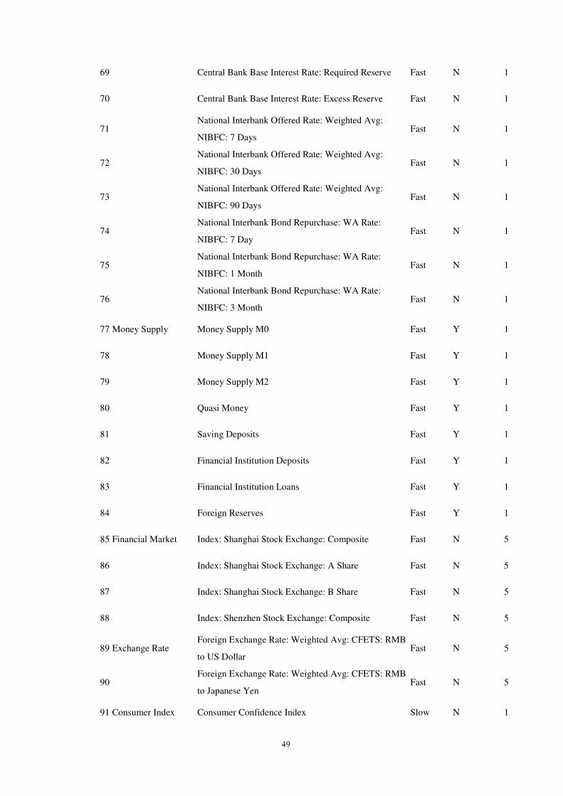
4. Data Description
Our sample consists of 100 monthly data series (1998M1 – 2010M2), and are
15
The program we employed in the estimation is based on Bernanke, Boivin and Eliasz (2005).

13
categorized into twelve groups.16
The first eleven groups focus on different aspects
of economic performance in China, including real activities, price index, investment,
government revenue and expenditure, retail sales, international trade, interest rate,
money aggregate, financial market, exchange rate and consumer index. With the
integration into the world economy, China is inevitably exposed to worldwide
economic uncertainties, especially that of the United States. Thus, the US data are
also included.
The data which are conceived to have seasonality are first adjusted by X-12 ARIMA.
The Augmented Dickey Fuller test is employed to test the stationarity of the data
series. In case of non-stationarity, the series will be transformed by first log
difference to attain stationarity. Following Bernank, Boivin and Eliasz (2005), we
distinguish two categories of data series in this paper, namely, fast-moving and
slow-moving data. Fast moving data, such as interest rates, monetary aggregates,
asset prices, exchange rate and consumer indexes, are contemporaneously affected
by a monetary shock. Slow moving data, including the data of real activity, price
level and international trade, are affected by a monetary shock for a lag of one
period.
5. Empirical Results
We estimate a Factor-Augmented VAR model with a number of
frequently-employed policy instruments, namely the repo rate, benchmark lending
rate, total financial institution loans and M2 to evaluate their respective
effectiveness. In addition, as the PBC usually uses several market-based instruments
16
A detailed description of each data series is presented in the appendix.

14
simultaneously to achieve its objectives, we also use a factor, which tracks a wide
range of market based policy instruments at the disposal of the PBC, to represent a
general stance of the monetary policy. By estimating the FAVAR with this policy
factor, we should observe the impacts on the economy from a sudden change, which
is a 25-basis-point innovation for the policy instrument, of the market-based
monetary stance. For each of the five models, we augment the VAR with three
factors.17
Besides, the exchange rate policy has undergone substantial reform since 2005. To
evaluate the change of the effectiveness from this reform, we estimate the models
with two different subsamples, which are January 1998 - June 2005 and September
2002 - February 2010. The first subsample covers the period before the exchange
rate reform while the second subsample covers the period under a more flexible
currency regime. By comparing the performance of monetary policy in the two
subsample periods, one could shed light on the evolution of monetary policy due to
a loosened control on the exchange rate. To understand the effects of a shock from
monetary policy on the economy, we also present the impulse response function for
a wide range of economic indicators along with the industrial output and consumer
price level.
5.1 Estimation of FAVAR with Repo Rate as the instrument
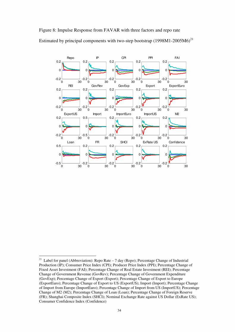
First, we estimate the model with the repo rate as the policy instrument. Figure 8
displays the resulting impulses response functions generated by the FAVAR before
17
Following Bernanke, Boivin, Eliazs (2005), we use FAVAR with three factors and one policy
instrument as the baseline model. Stock and Watson (1999, 2002b) also show that a few, perhaps two,
dynamic factors can account for a large amount of variation in the macroeconomic data series.
15
the exchange rate reform given an increase in the repo rate. The response of the
industrial production is insignificant18
. The consumer price index exhibits a
moderate increase initially but fall after a few months. The real estate investment
also plunges for an extended period of time. Consequently, the repo rate is
ineffective in promoting economic growth and weak at maintaining the price level
under the fixed exchange rate.
Figure 9 shows the impulse response function generated by FAVAR from
September 2002 to February 2010. Given a positive shock in repo rate, the industrial
production has gently come down a few months after the shock while the consumer
price index goes up for the fifteen months, displaying a sign of price puzzle. In
comparison with the response under a fixed exchange rate, the repo rate is more
capable of stimulating the real economic performance, but may not be an effective
tool in containing inflation.
[Insert Figure 8 here]
[Insert Figure 9 here]
5.2 Estimation of FAVAR with Benchmark Lending Rate as the instrument
In the second model, we estimate the response of industrial production and inflation
from a positive shock in the benchmark lending rate. Figure 10 depicts that the
industrial production is not responding to a contractionary monetary policy shock.
Though the price indexes are gently reduced, the reduction only lasts for fifteen
18
For the results figures (Figure 8-11, 14-19), the green line shows the point estimate of the
response function. The light blue line and the red line represent the 90% upper and lower confidence
level respectively.
16
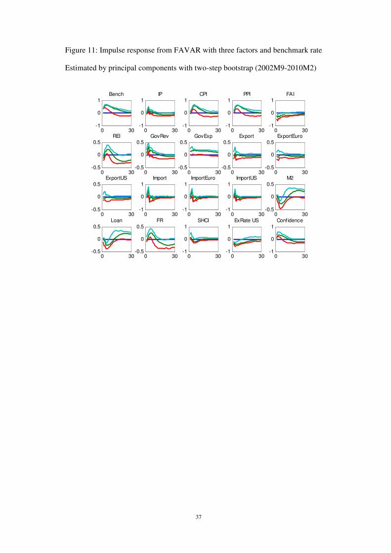
months. Figure 11 shows the response functions under a more flexible currency
regime. The industrial production responds with a prolonged and moderate
reduction to an upward shock of the interest rate. However, the price indexes soar,
resulting in price puzzles for about twenty months following a tightening policy
shock.
Before the exchange rate reform, both the repo rate and the benchmark lending rate
were not effective in stimulating the economic performance. When the central bank
raises the lending rate, the industrial production and price indexes show
insignificant and short-lived response in Figure 8 and Figure 10. When the exchange
rate is more relaxed, it has a mildly significant and long-lasting downward impact
on the industrial production after a few months of the shock, implying a more
effective policy to stimulate economic growth. Yet, the interest rates also give rise
the price puzzles for both the consumer and producer price indexes. Therefore, the
effectiveness of market-based monetary policy does not show any sign of
improvement given a more flexible exchange rate policy.
[Insert Figure 10 here]
[Insert Figure 11 here]
5.3 Estimation of FAVAR with the monetary factor as the instrument
Thirdly, we assess the impact of a change of market-based monetary stance by the
PBC on the real economy. As the monetary and financial markets have not been
fully liberalized, the transmission channels of the policy instrument are not as
efficient as those in the developed countries. The PBC has to rely on a number of
17
policy instruments simultaneously to influence the economy. We consider 15
market-based measures which are directly or indirectly managed by the PBC as
potential monetary instruments19
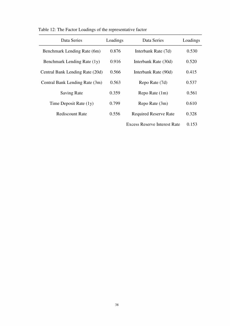
. We extract a policy factor from these 15 data
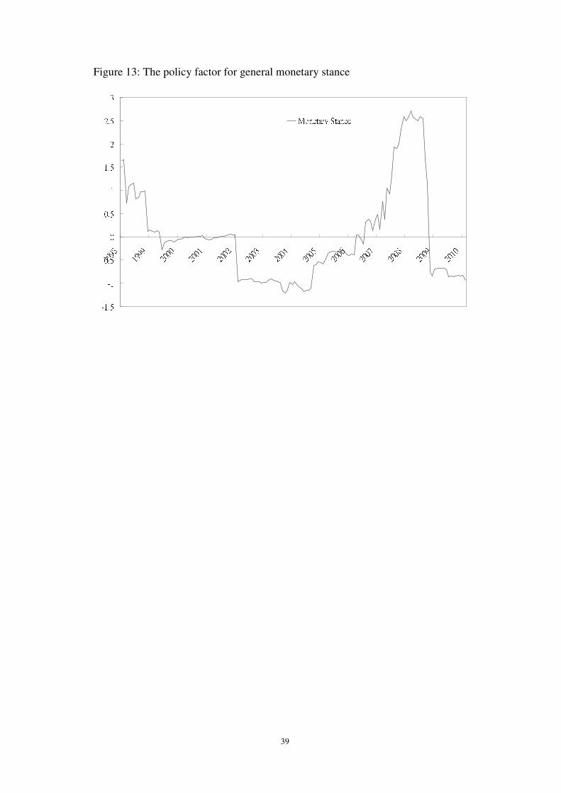
series by maximum likelihood estimation. Table 12 shows that this factor is
positively related to the interest rates. The movement of this policy factor, as
depicted in Figure 13, resembles those of the repo rate and benchmark lending rate.
As a result, an upward shock of this factor could be interpreted as a tightening
monetary stance.
[Insert Table 12 here]
[Insert Figure 13 here]
Figure 14 displays the impulse response functions from an upward shock of the
policy factor before the exchange rate reform. When the central bank takes a
contractionary monetary stance, the negative impact on industrial production and
price indexes are small but significant. These notable responses suggest a
combination of market-based instruments is more effective than a single instrument,
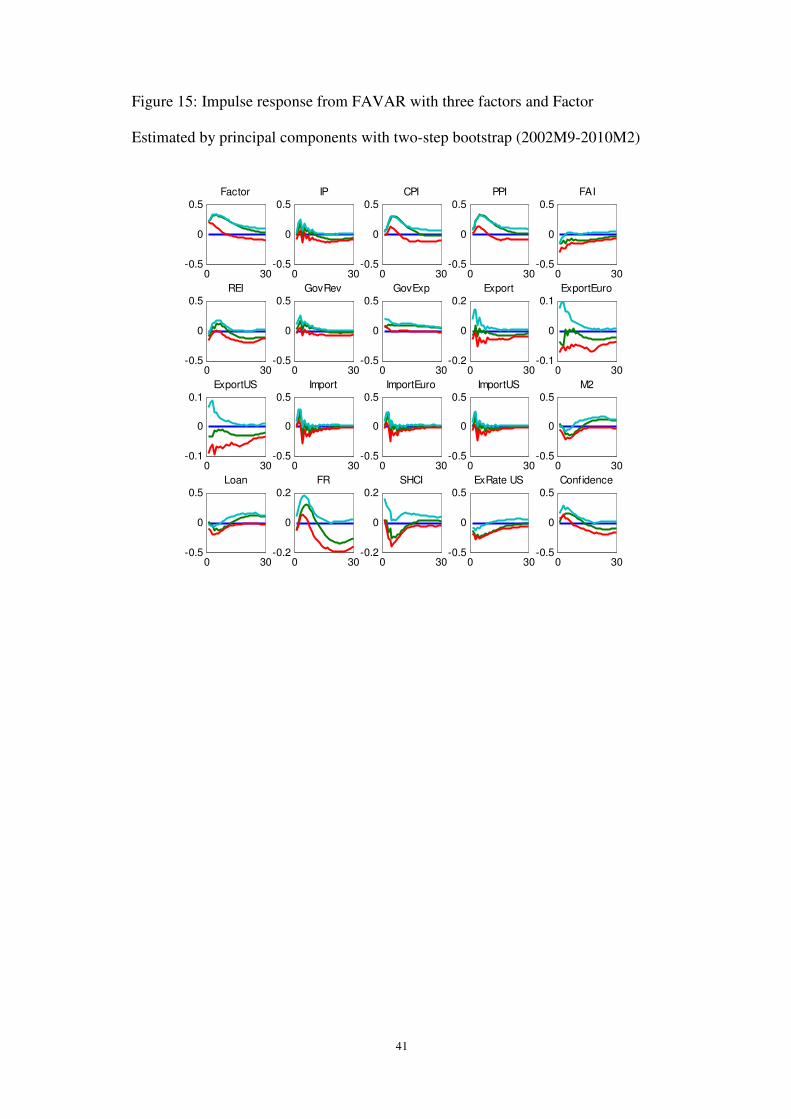
such as the repo rate or the benchmark rate. Besides, Figure 15 presents the impulse
responses generated from the FAVAR between September 2002 and February 2010.
Not surprisingly, a downward and persistent pressure on the industrial production is
building up after a few months of the onset of contractionary policy. Nonetheless,
the price puzzle in consumer price index emerges and prevails for nearly twenty
months.
19
These series include rediscount rate, repo rate (7 days, 1 month and 3 months), benchmark lending
rate (6 months and 1 year), central bank lending rate (20 days and 3 months), Interbank Interest Rate
(7 days, 30 days, 90 days) Interest rate on required reserve and excess reserve, saving rate and time
deposit rate (1y). All these 18 series are seasonally adjusted and stationary.
18
[Insert Figure 14 here]
[Insert Figure 15 here]
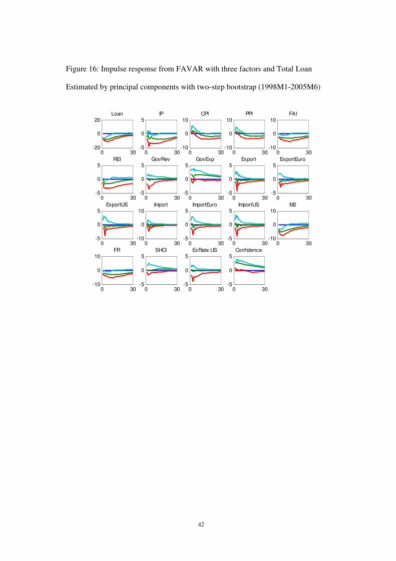
5.4 Estimation of FAVAR with total loan as the instrument
Other than market-based instruments, the PBC also employ non-market-based
instruments to prop up the economy and contain the price level. The total loan,
which is affected by both interest rates and the administrative measures, is a
principal indicator for the general monetary stance of the central bank. The PBC can
tighten bank lending by raising the interest rates or by window guidance. Figure 16
and Figure 17 show the impulse responses of economic variables to a lowering of
the growth rate of total loans. Under the fixed exchange rate (as shown in Figure 16),
a negative shock in total loan results in a rapid and persistent decline in industrial
production. The price indexes are also lowered a few months after the monetary
policy is tightened. When the exchange rate is more flexible, a decreased total loan
also hugely reduces the industrial production and consumer price index. These
results reveal that the control of total loan is highly effective in regulating the
economy.
[Insert Figure 16 here]
[Insert Figure 17 here]
5.5 Estimation of FAVAR with M2 as the instrument
For the last model, we estimate the impulse response functions of industrial
production and inflation for a downward shock in the growth rate of M2. Figure 18
19
shows that, under the pegged exchange rate regime, the M2 shock initiates mild
response from the industrial production and the consumer price index. This means
an increase in money supply can only play a role to stimulate the real economic
activities and raise the general price level. The impact of M2 on the economy has
also been explicit, though less significant, after the exchange rate reform. From
Figure 19, an increase in the growth rate of M2 can boost the industrial production
and the consumer price index but the impacts die out about 15 months after the
shock.
As compared to the estimation results of the repo rates and benchmark rates, the
growth rate of total loan and of money supply are more successful in managing the
real economic activity and price level. As explained in Section 2.2C and 2.2D, the
total loan and M2 can either be adjusted by varying the interest rates and by window
guidance. Neither the repo rate nor the benchmark rates, however, are shown to
have a significant impact on the M2 as depicted in Figures 8 and 10, implying that
the window guidance is the apparent driving force of the change of the money
supply.
[Insert Figure 18 here]
[Insert Figure 19 here]
5.6 Policy discussion
In the above estimation exercise, we could shed light on the policy implication in
two dimensions – the effectiveness of market-based and non-market-based

20
instruments, and the effectiveness of instruments under a fixed or more flexible
exchange rate regime. By comparing the results of different policy instruments, we
show that the growth rate of total loan and growth rate of money supply are more
effective than the interest-rate based monetary instruments in regulating the
economy. When quantity of loan or broad money supply grows at a higher rate, the
industrial production and consumer price index will follow with a rise immediately
after the shock. Nevertheless, the real economy and price level respond with a
longer lag and less significant amount to the shocks of repo rate and benchmark rate.
This shows that the central bank could not solely rely on the use of interest rates to
fine tune the economy. Window guidance and regulatory adjustment are still crucial
and effective to monetary policy implementation.
Our results also suggest that market-based policies have generally mild impacts on
industrial production and price level. There are several explanations for this. The
first is the high level of excess reserve in the banking industry (Green, 2005). The
high excess reserve ratio, about 4 percent from 2005 to 200720
, absorbs much of the
influence of the monetary policies. Secondly, the partially liberalized money market
also restrains the capacity of market-based policies. Though plenty of interest rate
liberalization reforms have been implemented in the past decades, the ceiling on
deposit rates and floor on lending rates are still in place, thus constraining the
capacity for effective monetary policy.
In addition, the policy factor which tracks the monetary stance for market-based
policies has a more pronounced impact on the economy than other monetary
instruments before the exchange rate reform in 2005. This suggests that a wide
20
In United States, the excess reserves are usually less than 2 percent of the deposit.
21
range of market-based monetary instruments is more effective to manage the
economy than a single interest rate adjustment.
Regarding the change of exchange rate regimes, our estimation results are less
explicit. As the Renminbi is fixed against US dollar before 2005, the Chinese
central bank can hardly set its monetary policy independent of its American
counterpart. Since the exchange rate reform in 2005, the Renminbi appreciated
significantly against the US dollar. When the PBC carries out market-based
tightening policies, the industrial production displays a more significant decline
under a more flexible exchange rate regime. Nevertheless, the price indexes rise
amid a monetary tightening condition in the second subsample. There are several
reasons for the emergence of price puzzles in the estimation. First, the Renminbi is
effectively repegged to US dollars since 2008. This highly restricts the sample size
for estimation in this paper. Besides, the central bank still relies heavily on the
window guidance as a principal monetary instrument, especially after the outbreak
of global financial crisis. Moreover, the emergence of price puzzles given a shock
from the market-based instruments may also suggest that those instruments are not
designed for fighting against inflation in China.
6. Conclusion
In order to have a better understanding of the monetary transmission mechanism in
China, this paper improves the conventional VAR model by including factor
variables. It is found that the interest rates and the market-based monetary policies
have little impact on the real economy and the price level under the fixed exchange
rate regime. These policy instruments become slightly more effective on the
22
industrial production when the exchange rate is more market determined. We also
track the market-based monetary stance of the PBC by summarizing 15 policy
variables in one policy factor. This policy factor is more effective than any
individual policy instrument, implying that the PBC may employ a wide range of
monetary instruments.
Admittedly, the market-based instruments are slightly more influential on the
economy under a more flexible currency regime. Nevertheless, the
non-market-based measures at the disposal of the central bank are much more
effective. These results are not surprising as the central bank could control the total
financial loans as well as the broad money supply with a higher flexibility than the
interest rates, which are highly restricted due to rigid currency regime. As a result,
China could still carry out effective monetary policy through non-market-based
measures under the rigid exchange rate system.

23
References
Belviso, F. and F. Milani, 2006, “Structural Factor-Augmented VARs and the
effects of monetary policy,” The B.E. Journal of Macroeconomics, 6(3).
Bernanke, B., J. Boivin, and P. Eliasz, 2005, “Measuring the Effects of Monetary
Policy: A Factor-Augmented Vector Autoregressive (FAVAR) Approach,”
Quarterly Journal of Economics, 120(1): 387-422.
Boivin, J. and M. Giannoni, 2006, “Has Monetary Policy Become More Effective?”
Review of Economics and Statistics, 88(3): 445-462.
Brandt, L. and X. D. Zhu (2002), “What Ails China: A Long-Run Perspective on
Growth and Inflation (or Deflation) in China,” East Asia in Transition: Economic
and Security Challenges, 49-72, University of Toronto Press.
Breitung, J. and Eickmeier, S. 2005. “Dynamic Factor Models,” Deutsche
Bundesbank Discussion Paper 38/2005.
Dickinson, D. and J. Liu, 2007, “The Real Effects of Monetary Policy in China: An
Empirical Analysis,” China Economic Review, 18(1): 87-111.
Du, J., Q. He, and O. Rui, 2010, “Does Financial Deepening Promote the Risk
Sharing in China,” Journal of the Asia Pacific Economy, forthcoming.
Favero, C., M. Marcellino, and F. Neglia, 2005, “Principal Components at Work:
24
The Empirical Analysis of Monetary Policy with Large Data Sets,” Journal of
Applied Econometrics, 20: 603-620.
Forni, M., D. Giannone, M. Lippi, and L. Reichlin, 2005, “The Generalized
Dynamic Factor Model: One-Sided Estimation and Forecasting,” Journal of the
American Statistical Association, 100: 830-840.
Forni, M., D. Giannone, M. Lippi, and L. Reichlin, 2009, “Opening the Black Box:
Structural Factor Models with Large Cross Sections,” Econometric Theory, 25(05):
1319-1347.
Goodfriend, M. and E. Prasad, 2007, “A Framework for Independent Monetary
Policy in China,” CESifo Economic Studies, 53(1): 2-41.
Green, S., 2005, “Making Monetary Policy Work in China: A Report from the
Money Market Front Line,” Manuscript, Standard Chartered Bank, Shanghai,
China.
He, Q., T. T. Chong, and K. Shi (2009), “What Accounts for Chinese Business
Cycle”, China Economic Review, 20, 650-661
Koivu, T., 2009, “Has the Chinese Economy Become More Sensitive to Interest
Rates? Studying Credit Demand in China,” China Economic Review, 20(3):
455-470.

25
Lardy, N., 2005, “Exchange Rate and Monetary Policy in China,” Cato Journal,
25(1): 41-47.
Laurens, B. and R. Maino, 2007, “China: Strengthening Monetary Policy
Implementation,” IMF Working Paper No. 07/14.
Mehrotra, A., 2007, “Exchange and Interest Rate Channels during a Deflationary
Era - Evidence from Japan, Hong Kong and China,” Journal of Comparative
Economics, 35: 188-210.
The People’s Bank of China, 2005, “Report on Steadily Progress in Interest Rate
Liberalization”.
The People’s Bank of China, 2007, “China Monetary Policy Report Quarter Four
2006”.
Park, A. and K. Sehrt, 2001, “Tests of Financial Intermediation and Banking
Reform in China,” Journal of Comparative Economics, 29(4): 608-644.
Peng, W., H. Chen, and W. Fan. 2006. “Interest Rate Structure and Monetary Policy
Implementation in Mainland China,” 1/06. China Economic Issue. HKMA
Prasad, E., Rumbaugh, T. and Wang, Q., 2005, “Putting the Cart before the Horse?
Capital Account Liberalization and Exchange Rate Flexibility in China,”
International Monetary Fund, IMF Policy Discussion Paper: No. 05/1,
26
Rudebusch, G., 1998, “Do Measures of Monetary Policy in a VAR make Sense?”
International Economic Review, 39(4): 907-931.
Sims, C., 1992, “Interpreting the Macroeconomic Time Series Facts,” European
Economic Review, 36(5): 975-1011.
Stock, J. and M. Watson, 1998, “Diffusion Indexes,” NBER Working Paper.
Stock, J. and M. Watson, 1999, “Forecasting Inflation,” Journal of Monetary
Economics, 44(2): 293-335.
Stock, J. and M. Watson, 2002a, “Forecasting using Principal Components from a
Large Number of Predictors,” Journal of American Statistical Association, 97(460):
1167-1179.
Stock, J. and M. Watson, 2002b, “Macroeconomic Forecasting using Diffusion
Indexes,” Journal of Business & Economic Statistics, 20(2): 147-162.
Stock, J. and M. Watson, 2005, “Implications of Dynamic Factor Models for VAR
Analysis,” NBER working paper.
Yi, G. 2008, “The Monetary Policy Transmission Mechanism in China,” In
Transmission Mechanisms for Monetary Policy in Emerging Market Economies,
179-181. Vol. 35: Bank for International Settlements.
27
Appendix I:
Figure 1. Repo Rate
012345678910
1998 1999 2000 2001 2002 2003 2004 2005 2006 2007 2008 2009 2010Percent
National Interbank Bond Repurchase: WA Rate: NIBFC: 7 Day
Source: CEIC Database

28
Figure 2: Benchmark Lending Rate (1 year)
012345678910
1998 1999 2000 2001 2002 2003 2004 2005 2006 2007 2008 2009 2010Percent
Base Lending Rate: Working Capital: 1 Year
Source: CEIC Database
29
Figure 3: Percentage Change of Financial Institution Loans (Year-on-year)
05101520253035
1998 1999 2000 2001 2002 2003 2004 2005 2006 2007 2008 2009 2010Percent
Growth rate of Financial Institution Loans
Source: CEIC Database

30
Figure 4: Percentage Change of Money Supply M2 (Year-on-year)
051015202530
1998 1999 2000 2001 2002 2003 2004 2005 2006 2007 2008 2009 2010Percent
Percentage Change of Money Supply M2
Source: CEIC Database
31
Figure 5: The Renminbi exchange rate against the US Dollar
0123456789
1998 1999 2000 2001 2002 2003 2004 2005 2006 2007 2008 2009 2010RMB/USD Foreign Exchange Rate: Weighted Avg: CFETS: RMB to US Dollar
Source: CEIC Database

32
Figure 6: Annual growth rate of Industrial Production
-505101520253035
1994 1995 1996 1997 1998 1999 2000 2001 2002 2003 2004 2005 2006 2007 2008 2009 2010Percent
Industrial Production Index: % Change
Source: CEIC Database

33
Figure 7: Annual inflation rate (Consumer Price Index)
-5051015202530
1994 1995 1996 1997 1998 1999 2000 2001 2002 2003 2004 2005 2006 2007 2008 2009 2010Percent
Consumer Price Index
Source: CEIC Database
34
Figure 8: Impulse Response from FAVAR with three factors and repo rate
Estimated by principal components with two-step bootstrap (1998M1-2005M6)21
0 30-0.2
0
0.2Repo
0 30-0.2
0
0.2IP
0 30-0.2
0
0.2CPI
0 30-0.2
0
0.2PPI
0 30-0.2
0
0.2FAI
0 30-0.2
0
0.2REI
0 30-0.2
0
0.2GovRev
0 30-0.2
0
0.2GovExp
0 30-0.2
0
0.2Export
0 30-0.2
0
0.2ExportEuro
0 30-0.2
0
0.2ExportUS
0 30-0.5
0
0.5Import
0 30-0.2
0
0.2ImportEuro
0 30-0.2
0
0.2ImportUS
0 30-0.2
0
0.2M2
0 30-0.5
0
0.5Loan
0 30-0.2
0
0.2FR
0 30-0.2
0
0.2SHCI
0 30-0.2
0
0.2ExRate US
0 30-0.2
0
0.2Confidence
21
Label for panel (Abbreviation): Repo Rate – 7 day (Repo); Percentage Change of Industrial
Production (IP); Consumer Price Index (CPI); Producer Price Index (PPI); Percentage Change of
Fixed Asset Investment (FAI); Percentage Change of Real Estate Investment (REI); Percentage
Change of Government Revenue (GovRev); Percentage Change of Government Expenditure
(GovExp); Percentage Change of Export (Export); Percentage Change of Export to Europe
(ExportEuro); Percentage Change of Export to US (ExportUS); Import (Import); Percentage Change
of Import from Europe (ImportEuro); Percentage Change of Import from US (ImportUS); Percentage
Change of M2 (M2); Percentage Change of Loan (Loan); Percentage Change of Foreign Reserve
(FR); Shanghai Composite Index (SHCI); Nominal Exchange Rate against US Dollar (ExRate US);
Consumer Confidence Index (Confidence)

35
Figure 9: Impulse Response from FAVAR with three factors and repo rate
Estimated by principal components with two-step bootstrap (2002M9-2010M2)
0 30-0.5
0
0.5Repo
0 30-0.2
0
0.2IP
0 30-0.2
0
0.2CPI
0 30-0.2
0
0.2PPI
0 30-0.1
0
0.1FAI
0 30-0.2
0
0.2REI
0 30-0.2
0
0.2GovRev
0 30-0.2
0
0.2GovExp
0 30-0.1
0
0.1Export
0 30-0.2
0
0.2ExportEuro
0 30-0.1
0
0.1ExportUS
0 30-0.2
0
0.2Import
0 30-0.2
0
0.2ImportEuro
0 30-0.2
0
0.2ImportUS
0 30-0.2
0
0.2M2
0 30-0.5
0
0.5Loan
0 30-0.2
0
0.2FR
0 30-0.1
0
0.1SHCI
0 30-0.2
0
0.2ExRate US
0 30-0.1
0
0.1Conf idence

36
Figure 10: Impulse response from FAVAR with three factors and benchmark rate
Estimated by principal components with two-step bootstrap (1998M1-2005M6)
0 30-0.5
0
0.5Bench
0 30-0.5
0
0.5IP
0 30-0.5
0
0.5CPI
0 30-0.5
0
0.5PPI
0 30-0.5
0
0.5FAI
0 30-0.5
0
0.5REI
0 30-0.5
0
0.5GovRev
0 30-0.5
0
0.5GovExp
0 30-1
0
1Export
0 30-0.5
0
0.5ExportEuro
0 30-1
0
1ExportUS
0 30-1
0
1Import
0 30-1
0
1ImportEuro
0 30-1
0
1ImportUS
0 30-0.5
0
0.5M2
0 30-0.5
0
0.5Loan
0 30-0.5
0
0.5FR
0 30-0.5
0
0.5SHCI
0 30-0.5
0
0.5ExRate US
0 30-1
0
1Confidence
37
Figure 11: Impulse response from FAVAR with three factors and benchmark rate
Estimated by principal components with two-step bootstrap (2002M9-2010M2)
0 30-1
0
1Bench
0 30-1
0
1IP
0 30-1
0
1CPI
0 30-1
0
1PPI
0 30-1
0
1FAI
0 30-0.5
0
0.5REI
0 30-0.5
0
0.5GovRev
0 30-0.5
0
0.5GovExp
0 30-0.5
0
0.5Export
0 30-0.5
0
0.5ExportEuro
0 30-0.5
0
0.5ExportUS
0 30-1
0
1Import
0 30-1
0
1ImportEuro
0 30-1
0
1ImportUS
0 30-0.5
0
0.5M2
0 30-0.5
0
0.5Loan
0 30-0.5
0
0.5FR
0 30-1
0
1SHCI
0 30-1
0
1ExRate US
0 30-1
0
1Confidence
38
Table 12: The Factor Loadings of the representative factor
Data Series Loadings Data Series Loadings
Benchmark Lending Rate (6m) 0.876 Interbank Rate (7d) 0.530
Benchmark Lending Rate (1y) 0.916 Interbank Rate (30d) 0.520
Central Bank Lending Rate (20d) 0.566 Interbank Rate (90d) 0.415
Central Bank Lending Rate (3m) 0.563 Repo Rate (7d) 0.537
Saving Rate 0.359 Repo Rate (1m) 0.561
Time Deposit Rate (1y) 0.799 Repo Rate (3m) 0.610
Rediscount Rate 0.556 Required Reserve Rate 0.328
Excess Reserve Interest Rate 0.153
39
Figure 13: The policy factor for general monetary stance
-1.5-1-0.500.511.522.53
1998 1999 2000 2001 2002 2003 2004 2005 2006 2007 2008 2009 2010Monetary Stance

40
Figure 14: Impulse response from FAVAR with three factors and Factor
Estimated by principal components with two-step bootstrap (1998M1-2005M6)
0 30-0.5
0
0.5Factor
0 30-0.5
0
0.5IP
0 30-0.5
0
0.5CPI
0 30-0.5
0
0.5PPI
0 30-0.5
0
0.5FAI
0 30-0.5
0
0.5REI
0 30-0.2
0
0.2GovRev
0 30-0.5
0
0.5GovExp
0 30-0.5
0
0.5Export
0 30-0.2
0
0.2ExportEuro
0 30-0.2
0
0.2ExportUS
0 30-0.5
0
0.5Import
0 30-0.5
0
0.5ImportEuro
0 30-0.5
0
0.5ImportUS
0 30-0.5
0
0.5M2
0 30-0.5
0
0.5Loan
0 30-0.5
0
0.5FR
0 30-0.5
0
0.5SHCI
0 30-0.2
0
0.2ExRate US
0 30-0.5
0
0.5Confidence
41
Figure 15: Impulse response from FAVAR with three factors and Factor
Estimated by principal components with two-step bootstrap (2002M9-2010M2)
0 30-0.5
0
0.5Factor
0 30-0.5
0
0.5IP
0 30-0.5
0
0.5CPI
0 30-0.5
0
0.5PPI
0 30-0.5
0
0.5FAI
0 30-0.5
0
0.5REI
0 30-0.5
0
0.5GovRev
0 30-0.5
0
0.5GovExp
0 30-0.2
0
0.2Export
0 30-0.1
0
0.1ExportEuro
0 30-0.1
0
0.1ExportUS
0 30-0.5
0
0.5Import
0 30-0.5
0
0.5ImportEuro
0 30-0.5
0
0.5ImportUS
0 30-0.5
0
0.5M2
0 30-0.5
0
0.5Loan
0 30-0.2
0
0.2FR
0 30-0.2
0
0.2SHCI
0 30-0.5
0
0.5ExRate US
0 30-0.5
0
0.5Confidence
42
Figure 16: Impulse response from FAVAR with three factors and Total Loan
Estimated by principal components with two-step bootstrap (1998M1-2005M6)
0 30-20
0
20Loan
0 30-5
0
5IP
0 30-10
0
10CPI
0 30-10
0
10PPI
0 30-10
0
10FAI
0 30-5
0
5REI
0 30-5
0
5GovRev
0 30-5
0
5GovExp
0 30-5
0
5Export
0 30-5
0
5ExportEuro
0 30-5
0
5ExportUS
0 30-10
0
10Import
0 30-5
0
5ImportEuro
0 30-5
0
5ImportUS
0 30-10
0
10M2
0 30-10
0
10FR
0 30-5
0
5SHCI
0 30-5
0
5ExRate US
0 30-5
0
5Confidence

43
Figure 17: Impulse response from FAVAR with three factors and Total Loan
Estimated by principal components with two-step bootstrap (2002M9-2010M2)
0 30-10
0
10Loan
0 30-10
0
10IP
0 30-5
0
5CPI
0 30-5
0
5PPI
0 30-5
0
5FAI
0 30-10
0
10REI
0 30-10
0
10GovRev
0 30-5
0
5GovExp
0 30-5
0
5Export
0 30-5
0
5ExportEuro
0 30-5
0
5ExportUS
0 30-5
0
5Import
0 30-5
0
5ImportEuro
0 30-5
0
5ImportUS
0 30-10
0
10M2
0 30-5
0
5FR
0 30-5
0
5SHCI
0 30-5
0
5ExRate US
0 30-5
0
5Confidence
44
Figure 18: Impulse response from FAVAR with three factors and M2
Estimated by principal components with two-step bootstrap (1998M1-2005M6)
0 30-20
0
20M2
0 30-10
0
10IP
0 30-5
0
5CPI
0 30-5
0
5PPI
0 30-10
0
10FAI
0 30-5
0
5REI
0 30-10
0
10GovRev
0 30-5
0
5GovExp
0 30-10
0
10Export
0 30-5
0
5ExportEuro
0 30-5
0
5ExportUS
0 30-10
0
10Import
0 30-10
0
10ImportEuro
0 30-10
0
10ImportUS
0 30-10
0
10FR
0 30-10
0
10SHCI
0 30-5
0
5ExRate US
0 30-10
0
10Confidence

45
Figure 19: Impulse response from FAVAR with three factors and M2
Estimated by principal components with two-step bootstrap (2002M9-2010M2)
0 30-10
0
10M2
0 30-10
0
10IP
0 30-5
0
5CPI
0 30-5
0
5PPI
0 30-5
0
5FAI
0 30-5
0
5REI
0 30-10
0
10GovRev
0 30-5
0
5GovExp
0 30-10
0
10Export
0 30-10
0
10ExportEuro
0 30-5
0
5ExportUS
0 30-10
0
10Import
0 30-5
0
5ImportEuro
0 30-5
0
5ImportUS
0 30-5
0
5FR
0 30-5
0
5SHCI
0 30-5
0
5ExRate US
0 30-5
0
5Confidence

46
Appendix II:
The time series data are all taken from CEIC Database. All of the series are monthly
data from January 1998 to August 2009. Each of the series is labeled as either fast
or slow. The transformation code: 1 – No transformation and 5 – First Difference of
Logarithm. The seasonally adjusted: SA – Seasonally adjusted by Census X-12,
NSA – Not seasonally adjusted.
No. Category Item Fast/Slow SA TC
1 Real Activities Industrial Production Index: % Change Y 1
2 Industrial Production: Salt Slow Y 5
3 Industrial Production: Canned Food Slow Y 5
4 Industrial Production: Cloth Slow Y 5
5 Industrial Production: Household Refrigerator Slow Y 5
6 Industrial Production: Automobiles Slow Y 5
7 Industrial Production: Motor Cycles Slow Y 5
8 Industrial Production: Air Conditioner Slow Y 5
9 Industrial Production: Televison Sets: Colour Slow Y 5
10 Industrial Production: Camera Slow Y 5
11 Industrial Production: Micro Computer Slow Y 5
12 Industrial Production: Plastic Products (PP) Slow Y 5
13 Industrial Production: Cement Slow Y 5
14 Industrial Production: Steel Slow Y 5
15 Production of Primary Energy: COAL Slow Y 5
16 Industrial Production: Coke Slow Y 5
17 Industrial Production: Rubber Tyre Slow Y 5
18 Industrial Production: Processed Crude Oil Slow Y 5

47
19 Industrial Production: Diesel Oil Slow Y 5
20 Industrial Production: Bicyles Slow Y 5
21 Industrial Production: Sewing Machines Slow Y 5
22 Industrial Production: Hi Fi Slow Y 5
23 Industrial Production: Household Washing Machines Slow Y 5
24 Industrial Production: Sugar Slow Y 5
25 Industrial Production: Synthetic Detergents Slow Y 5
26 Industrial Production: Kerosene Slow Y 5
27 Industrial Production: Sulphuric Acid Slow Y 5
28 Industrial Production: Chemical Fertilizer(100%
purity) Slow Y 5
29 Industrial Production: Plated Glass Slow Y 5
30 Industrial Production: Freight Wagons Slow Y 5
31 Industrial Production: Cloth: Pure Cotton Slow Y 5
32 Industrial Production: Civil Steel Ships Slow Y 5
33 Industrial Sales Slow Y 5
34 Industrial Sales: Heavy Industry Slow Y 5
35 Price Index Consumer Price Index Slow Y 1
36 Consumer Price Index: Food Slow Y 1
37 Consumer Price Index: Food: Grain Slow Y 1
38 Consumer Price Index: Clothing Slow Y 1
39 Consumer Price Index: Residence Slow Y 1
40 Consumer Price Index: Medicines and Medical Slow Y 1
41 Retail Price Index Slow Y 1
42 Retail Price Index: Food Slow Y 5
43 Producer Price Index: Industrial Products Slow Y 1

48
44 PPI: IP: Consumer Goods Slow Y 1
45 Purchasing PI: Raw Materials (RM): Total Slow Y 1
46 Purchasing PI: RM: Fuels and Power Slow Y 1
47 Investment Fixed Assets Investment: ytd Slow Y 1
48 FDI: Utilized: ytd: Total Slow Y 1
49 Real Estate Investment: ytd: Total Slow Y 1
50 Real Estate Inv: ytd: Residential Buildings Slow Y 1
51 Government Government Revenue Slow Y 1
52 Government Expenditure Slow Y 1
53 Retail Sales Retail Sales of Consumer Goods: Total Slow Y 1
54 International Trade Exports fob Slow Y 5
55 Exports: Europe Slow Y 5
56 Exports: USA Slow Y 5
57 Exports: ASEAN Slow Y 5
58 Imports cif Slow Y 5
59 Imports: Europe Slow Y 5
60 Imports: United States Slow Y 5
61 Imports: ASEAN Slow Y 5
62 Interest Rate Policy Rate: Month End: Rediscount Fast N 1
63 Savings Deposits Rate Fast N 1
64 Time Deposits Rate: 1 Year Fast N 1
65 Central Bank Base Interest Rate: Less Than 20 Days Fast N 1
66 Central Bank Base Interest Rate: 3 Months or Less Fast N 1
67 Base Lending Rate: Working Capital: 6 Months Fast N 1
68 Base Lending Rate: Working Capital: 1 Year Fast N 1
49
69 Central Bank Base Interest Rate: Required Reserve Fast N 1
70 Central Bank Base Interest Rate: Excess Reserve Fast N 1
71 National Interbank Offered Rate: Weighted Avg:
NIBFC: 7 Days Fast N 1
72 National Interbank Offered Rate: Weighted Avg:
NIBFC: 30 Days Fast N 1
73 National Interbank Offered Rate: Weighted Avg:
NIBFC: 90 Days Fast N 1
74 National Interbank Bond Repurchase: WA Rate:
NIBFC: 7 Day Fast N 1
75 National Interbank Bond Repurchase: WA Rate:
NIBFC: 1 Month Fast N 1
76 National Interbank Bond Repurchase: WA Rate:
NIBFC: 3 Month Fast N 1
77 Money Supply Money Supply M0 Fast Y 1
78 Money Supply M1 Fast Y 1
79 Money Supply M2 Fast Y 1
80 Quasi Money Fast Y 1
81 Saving Deposits Fast Y 1
82 Financial Institution Deposits Fast Y 1
83 Financial Institution Loans Fast Y 1
84 Foreign Reserves Fast Y 1
85 Financial Market Index: Shanghai Stock Exchange: Composite Fast N 5
86 Index: Shanghai Stock Exchange: A Share Fast N 5
87 Index: Shanghai Stock Exchange: B Share Fast N 5
88 Index: Shenzhen Stock Exchange: Composite Fast N 5
89 Exchange Rate Foreign Exchange Rate: Weighted Avg: CFETS: RMB
to US Dollar Fast N 5
90 Foreign Exchange Rate: Weighted Avg: CFETS: RMB
to Japanese Yen Fast N 5
91 Consumer Index Consumer Confidence Index Slow N 1

50
92 Consumer Expectation Index Slow N 1
93 Consumer Satisfactory Index Slow N 1
94 US Data M2 Money Stock (NSA) Slow Y 5
95 Commercial and Industrial Loans at All Commercial
Banks Slow Y 1
96 3-Month Treasury Bill: Secondary Market Rate Slow N 1
97 Producer Price Index: All Commodities Slow Y 1
98 Consumer Price Index for All Urban Consumers: All
Items Slow Y 1
99 Disposable Personal Income Slow Y 1
100 Personal Consumption Expenditures Slow Y 1