a fast-convergent modulation integral observer for online ... · discrete kalman filtering (dkf)...

0885-8993 (c) 2016 IEEE. Personal use is permitted, but republication/redistribution requires IEEE permission. See http://www.ieee.org/publications_standards/publications/rights/index.html for more information.

This article has been accepted for publication in a future issue of this journal, but has not been fully edited. Content may change prior to final publication. Citation information: DOI 10.1109/TPEL.2016.2570821, IEEETransactions on Power Electronics

TPEL-Reg-2015-08-1362 1

Abstract— Harmonics detection is a critical element of active

power filters. A previous review has shown that the Recursive

Discrete Fourier Transform and the Instantaneous p-q Theory are

effective solutions to extracting power harmonics in single-phase

and three-phase power systems, respectively. This paper presents

the operating principle of a new modulation function integral

observer algorithm that offers a fast solution for the extraction of

the fundamental current and the total harmonic current when

compared with existing methods. The proposed method can be

applied to both single- and three-phase systems. The observer-

based algorithm has an advantageous feature of being able to be

tuned offline for a specific application, having fast convergence

and producing estimated fundamental component with high

circularity. It has been tested with both simulations and practical

measurements for extracting the total harmonic current in a

highly efficient manner. The results have confirmed that the

proposed tool offers a new and highly effective alternative to the

smart grid industry.

Index Terms— fundamental extraction, harmonics detection,

active power filters

I. INTRODUCTION

onlinear electric loads draw non-sinusoidal currents from

the power supplies. Such harmonics have been identified

as key factor for poor power quality and a range of adverse

effects, including but not limited to, electromagnetic

interference (EMI), overheating of cables, and low power

factors [1]-[4]. Since the 1980’s, the power electronics research

community has responded with the solutions of active power

filters (APF) to deal with the power harmonics problems [5]-

[10]. In a typical setup of an active filter as shown in Fig.1, one

critical element is the real-time detection of the harmonic

current. The control block involves a fast harmonic current

detection so that a reference of the harmonic current can be

derived for the power inverter to inject the harmonic current

into the power line.

Despite such APF technologies have been

commercialized [11], active research is still on-going in

searching for effective real-time harmonics detection methods.

In a recent survey [12], it is stated that “There exist many

implementations supported by different theories (either in time-

or frequency-domain), which continuously debate their

performances proposing ever better solutions.” The survey [12]

provides a comprehensive comparison on six different methods

covering (i) Discrete Fourier Transform (DFT), (ii) Recursive

DFT, (iii) Synchronous Fundamental dq-Frame, (iv) 5th

Harmonic dq-Frame, (v) p-q Theory and (vi) 5th Generalized

Integrator. Methods (i), (ii) and (vi) are suitable for single-phase

systems, and hence are suitable for three-phase ones as well.

Methods (iii), (iv) and (v) can only be applied for three-phase

systems and require filtering. In terms of settling time and phase

error, the Recursive DFT and the p-q Theory methods offer

better performance than the others in the comparison.

Fig.1 A typical setup of an Active Power Filter

A Fast-Convergent Modulation Integral

Observer for Online Detection of the

Fundamental and Harmonics in Grid-Connected

Power Electronics Systems

Boli Chen, Gilberto Pin, Wai Man Ng, Member, IEEE, Thomas Parisini, Fellow, IEEE,

and S.Y. Ron Hui, Fellow, IEEE

N

Manuscript received August 11 2015; accepted May 6 2016. This work was

supported in part by the Hong Kong Research Council under the Theme-based Research Fund T23-701/14-N.

Boli Chen is with the Department of Electrical & Electronic Engineering,

Imperial College London (e-mail: [email protected]). G. Pin is with Electrolux, Italy (e-mail: [email protected]).

W.M. Ng is with the Department of Electrical & Electronic Engineering,

The University of Hong Kong (e-mail: [email protected]). T. Parisini is with the Department of Electrical & Electronic Engineering,

Imperial College London (e-mail: [email protected]).

S.Y.R. Hui is with Department of Electrical & Electronic Engineering, The University of Hong Kong (e-mail: [email protected]) and also with Imperial

College London (e-mail: [email protected]).

mailto:[email protected]

mailto:[email protected]



TPEL-Reg-2015-08-1362 2

The methods described in [12] are familiar ones in the power

electronics and power systems communities. However,

significant progress has been achieved in signal processing and

some of the emerging signal-processing methods are also

applicable to harmonics detection. The frequency domain

detection methods, such as discrete-time Fourier transform

(DFT) and the sliding DFT [14]-[17] represent the most

commonly used techniques for their fast convergence speed

and higher accuracy comparing to the time-domain methods.

Despite their successful applications, the existing methods

based on DFT also suffer from two main drawbacks: (1) a

synchronous sampling is needed, (2) problems in processing the

inter-harmonics may occur. On the other hand, in the time-

domain, methods like the Kalman filter, adaptive Notch filter

(ANF), Phase-locked-loop (PLL) and second-order

generalized integrators (SOGI) are proposed. These methods

usually ensure enhanced noisy immunity at the expense of

longer transient time than frequency-domain algorithms [18]-

[25]. Moreover, the implementation of time-domain methods

is more instrumental in the context of real-time harmonic

compensation. In [26], PLL, recursive DFT (RDFT), and

discrete Kalman filtering (DKF) from aforementioned two

categories are compared analytically in terms of real-time

implementation.

Very recently, a novel modulation-function integral observer

(MF observer) has been developed for general single-input

single-output linear systems. It offers practically instantaneous

convergence without high gain injection and complexity [27].

The novel theory reported in [27] is supported by a rigorous and

rather complex mathematical analysis. Thus, it may not be

obvious to power electronics engineers without the relevant

theoretical background. It is the aim of this paper to explore the

use of this new modulation integral observer for extracting the

fundamental current and the total harmonic current, the

knowledge of the latter being required in active power filtering

applications. The practical relevance of this MF observer with

active power filter applications is explained in this paper for the

first time. It is discovered that this new method, although

unknown to the power electronics and power system

communities, can perform fundamental current and total

harmonic current extraction quickly even in presence of

unknown dc offsets. The fast-convergent MF observer is

implemented in non-selective form to achieve a low

computational burden for on-line total harmonics extraction.

As confirmed by the simulation and experimental results, this

new method is favorably compared with some of the best

harmonics extraction methods commonly used in the active

power filtering applications.

II. BRIEF SUMMARY OF FREQUENCY-DOMAIN AND TIME-

DOMAIN HARMONIC DETECTION METHODS

Although conducted 10 years ago, the review in [12] still

provides some important insights into the operating principles

and the algorithm structures of different harmonic detection

methods. In this section, the schematics of the main methods

are used to highlight the differences of the methodologies in

terms of their algorithm structures. The understanding of such

differences and the schematic structures of the harmonic

detection algorithms will form a basis for comparing various

approaches, including the fast-convergent integral observer

under investigation in this paper.

A. Frequency-Domain Discrete Fourier Transform and

Recursive DFT

Fig.2 Schematic of the Discrete Fourier Transform

Fig.2 shows the schematic of the DFT method. The

Recursive DFT (RDFT) is similar to the DFT, except that the

samples are obtained within a moving window of the sampled

data. Note that the DFT method and its variants require the

measurements of the current only. There is no need to

measure the mains voltage. Its ability to handle 1-phase

measurements naturally indicates that it can be applied to a

3-phase system. There are two ways to work out the total

harmonic current.

The first one is to obtain the sum of the dc component

and fundamental component. By subtracting this sum

from the input current waveform, the total harmonic

current function can be obtained.

The second way is to add several of the low-order

current harmonic components together to form an

approximate harmonic current.

B. Time-Domain dq-Frame methods

Unlike the DFT method, the time-domain dq-Frame

approach requires the measurements of both of the mains

voltages and currents for the 3 phases. Therefore, this method

requires more sensors and is not suitable for single-phase

applications. The phase currents are measured and

transformed into the direct (d) and quadrature (q)

components. The time-domain dq-Frame method can also be

used in two ways as described for the DFT method.

(i) Synchronous fundamental dq-Frame method

Fig.3 shows the schematic of this method for

extracting the harmonic components. The rotating frame of

this method rotates at the fundamental frequency. This makes

the fundamental component appearing as the dc component

after the transformation in the rotating frame. With the use of

a high-pass filter with a typical bandwidth of 25Hz to120Hz,

the fundamental d- and q- current components can be

eliminated. The high-pass-filter enables the d- and q-

components of the harmonic currents (id~ and iq~) to go

through. By doing a dq-abc transformation, the harmonic

currents of the three phases can be re-constructed as ia*, ib*

and ic* in Fig.3.



TPEL-Reg-2015-08-1362 3

Fig.3 Schematic of the Synchronous Fundamental dq-Frame method

(ii) Synchronous harmonic dq-Frame method

The schematic of the harmonic dq-Frame is shown in

Fig.4. Again, the three phase currents and voltages have to be

measured. The procedures for extracting the harmonic

currents are similar to that of the fundamental dc frame

method. The major difference is that the rotating frames for

the harmonics will be according to their respectively

harmonic frequencies. Once the harmonic currents are

obtained, they can be added together to form the total

harmonic current. In practice, only several of the low-order

harmonic currents are usually used to reconstruct a good

approximation of the total harmonic currents for the three

phases.

It is important to note that the Fundamental dq-Frame

and Harmonic dq-Frame methods require the use of high-

pass or low-pass filters in the process of deriving the required

current components. Consequently, such approach

unavoidably introduces phase error, as previously discussed

in [12].

Fig.4 Schematic of the Synchronous Harmonic dq-Frame

(iii) Instantaneous p-q power theory

Another common approach for harmonic extraction is

based on the instantaneous p-q power theory pioneered by

Prof. Akagi [28]. The schematic is shown in Fig.5. Like the

dq-Frame methods, this approach needs the measurements of

the phase currents and voltages. Thus, it is suitable for 3-

phase systems, but not for single-phase ones. The phase

voltage and current measurements are transformed into their

respectively α and β components. Then the real power (p) and

reactive power (q) are obtained. With the use of high-pass

filters, the harmonic real power ( p~ ) and harmonic reactive

power ( q~ ) are obtained. The α and β harmonic current

components (*

i and *

i ) are then derived, and are eventually

used to reconstruct the total harmonic currents for the three

phases.

Fig.5 Schematic of the method based on the Instantaneous p-q Power Theory

In the next section, the proposed fast fundamental and

harmonics estimator will be illustrated.

III. MODULATION FUNCTION INTEGRAL OBSERVER METHOD

In In this section, a third-order MF observer is introduced for

harmonic current extraction. The schematic of this method is

shown in Fig.6. With the help of a modulation function that can

be selected and tuned offline for a specific application, the line

current samples are fed to the integral observer in order to

obtain the sum of the dc component and the fundamental

component of the current. The total harmonic current can then

be derived by subtracting this sum from the line current. It

should be noted that this method can be applied to a single-

phase system. Therefore, it can be applied to 3-phase ones too.

A The Modulation Function Integral Observer

Fig.6 Schematic of the fast-convergent Modulation Function Integral Observer

The line current i(t) is expressed as:

N

k

k titicti2

1 (1)

where c is the dc current component, t is the time variable, 𝑖1(𝑡) is the fundamental current, 𝑖𝑘(𝑡) is the kth current harmonic

component and

N

k

k ti2

is the total harmonic current.

Let the fundamental current be:

tati sin1 (2)

and

ticty 1 (3)

where A is the amplitude of the fundamental current, is the

angular frequency and is the phase shift. It is important to

note that the integral observer considers the total harmonic

current as ‘noise’ initially. If 𝑦(𝑡) can be found by the observer,

from (1) and (3), the total harmonic current can be obtained

easily “by subtraction” as follows:



TPEL-Reg-2015-08-1362 4

tytitiN

k

k 2

(4)

Therefore, 𝑦(𝑡) is chosen to be the single output of the

integral observer introduced in the following lines.

Differentiating (3) twice leads to:

tity 1

2 (5)

where ty is the second-order time-derivative of y(t). Based

on (3) and (5), one can form the following expression:

ti

c

ty

ty

1

20

11

(6)

Now, assume that the single output 𝑦(𝑡) is generated by a

general 3rd order state-space observable system,

tty

ttT

Z

Z

zc

zAz (7)

where we let

𝐳(𝑡) = [

𝑧1(𝑡)𝑧2(𝑡)

𝑧3(𝑡)]

= [𝑐 + 𝑎 sin(𝜔𝑡 + 𝜑)

𝜔 cos(𝜔𝑡 + 𝜑)

𝜔2𝑐

] (8)

and

000

10

0102zA ,

0

0

1

Zc

It can be easily seen that

tytz 1 (9)

tytytz 2

3 (10)

Clearly, the total harmonic current can be derived as long as

𝑧1(𝑡) is available. However, in the following lines, we will

show that the dc offset and the fundamental signal can be

individually recovered by using the state vector 𝐳(𝑡). Since only

tz1 and tz3 are relevant in the calculation, the following

matrix equations can be derived:

tt Ayze (11)

where

tz

tzt

3

1

ez ,

1

012

A and

ty

tyt

y

thus leading to

tt ezAy1 (12)

The 2×1 state column vector tez can be related to the 3×1

state column vector tz as:

tt zIz ee (13)

with

100

001eI

In view of (13), (12) and (6), the fundamental and the dc

component modelled in the right hand side of (6) can be

retrieved by simple algebra (see A.3-A.5 in Appendix I).

B The Modulation Function and the Modulation Matrix

The modulation integral observer uses a set of the time-

monomial modulating functions (see [27]). In the case

addressed in this paper, the specific functions take on the form

!2

2

hn

twt

hn

h

h

for nh ,...,2,1 (14)

where n is the order of the system (i.e., n = 3 for the 3rd order

observer in this case) and 𝑤ℎ > 0 is a suitable positive

weighting factor. According to [27], the chosen modulation

functions must satisfy:

0

0

dt

d h

n (15)

The reason for selecting the modulation function (14) that is

characterized by condition (15) is provided in the Appendix II.

With the modulation function selected, the modulation

function matrix is defined as:

ttt

ttt

ttt

t

333

222

111

Γ (16)

where th and th

are the first and second derivatives of

th for 3,2,1h . For any choice of 𝑤ℎ, it holds that

𝜙1(𝑡) ≠ 𝜙2(𝑡) ≠ 𝜙3(𝑡), ∀𝑡 > 0

��1(𝑡) ≠ ��2(𝑡) ≠ ��3(𝑡), ∀𝑡 > 0

��1(𝑡) ≠ ��2(𝑡) ≠ ��3(𝑡), ∀𝑡 > 0

thus tΓ is invertible for any 𝑡 > 0.

Remarks:

Although 𝜙ℎ(𝑡), ℎ = 1,2,3 are monotonically increasing

functions with respect to 𝑡, they are only computed over 0 ≤𝑡 ≤ 𝑇Δ + 𝑇𝑟 due to the action of reset (which is described later

on), thus evading the issue of data overflow. In this respect,

excessively large 𝑤ℎ is not advisable. The same rule is

applicable to ��ℎ(𝑡) and ��ℎ(𝑡). Moreover, by observing the

pattern of 𝚪(𝑡), 𝑤ℎ , ℎ = 1,2,3 should be chosen such that the

resultant 𝜙ℎ(𝑡), ℎ = 1,2,3 are enough separated to facilitate

the computation of matrix inverse). It is also important to note

that the elements in the matrix of (17) can be pre-determined

in an offline manner in the interval: 0 ≤ 𝑡 ≤ 𝑇Δ + 𝑇𝑟 .

Therefore, the matrix inversion is done only once. These pre-

determined values can be stored in memory for real-time

implementation.

With the availability of the modulation function matrix, the

following matrix equation can be formed:



TPEL-Reg-2015-08-1362 5

tz

tz

tz

ttt

ttt

ttt

tv

tv

tv

3

2

1

333

222

111

3

2

1

Hence,

tv

tv

tv

ttt

ttt

ttt

tz

tz

tz

3

2

1

1

333

222

111

3

2

1

(17a)

ttt φvΓz1)( (17b)

where the elements of column vector

Ttvtvtvt 321 φv can be obtained from

the practical measurements of the line current i(t). It follows

that

diitv

t

hφh 0

2 (18)

Thus, titttv hhφh 2 (19)

By observation (19), in order to avoid error-accumulation due

to the integration in case the measurement of 𝑖(𝑡) is noisy, we

adopt a discrete-time deflation strategy which is described in

the following lines. Let us define the time variable

tk =TD + k+1( )Tr (20)

where 𝑇Δ is the initial time, Tr is a repetitive period (note:

within each repetitive period are many small sampling

periods), and k is a natural number, the first derivative of

tv h can be obtained from the practical measurement of the

line current i(t). When k = 0, t = t0 = T + Tr, this forms the first

repetitive period. Beyond this time, the time variable lies

within the next repetitive period Tr (i.e. tk < t < tk+1).

1

2

0

2

for

0for

kkkk

httttiTttTtt

tttitttv

(21)

The time integrals of tv h in (21) will lead to the values of

tv h for h={1,2,3}. At the alternation of each repetitive

period, the values of tv h should be reset as:

kkr

T

hkh tttTTTtv

for 1

φvΓΓΕ

(22)

where

0

0

1

1Ε ,

0

1

0

2Ε and

1

0

0

3Ε .

Note that the line current is sampled at a relatively

high speed within each repetitive period, and the integral

values of (21) can provide the time-domain vector tφv

continuously at each sampling instant, then the state vector

tz can be obtained from (17).

1

1

0

1

for

for

kkk ttttttt

ttTttt

φ

φ

vΓ

vΓz

(23)

where T is a small time. It is needed because the modulation

function matrix is not invertible at t=0. Thanks to (9),

𝑧1(𝑡) represents an estimate of 𝑦(𝑡), then the total harmonic

current can be obtained from (4). In the practical

implementation, the proposed integral observer algorithms can

be discretized as shown in the Appendix I.

.

IV. SIMULATION STUDY OF CONVERGENT RATES AND

TRACKING ERRORS

In order to evaluate the performance of the methods under

consideration, a simulation study based on the conditions

similar to those set in [12] has been conducted. The

characteristic of the line currents are tabulated in Table I and

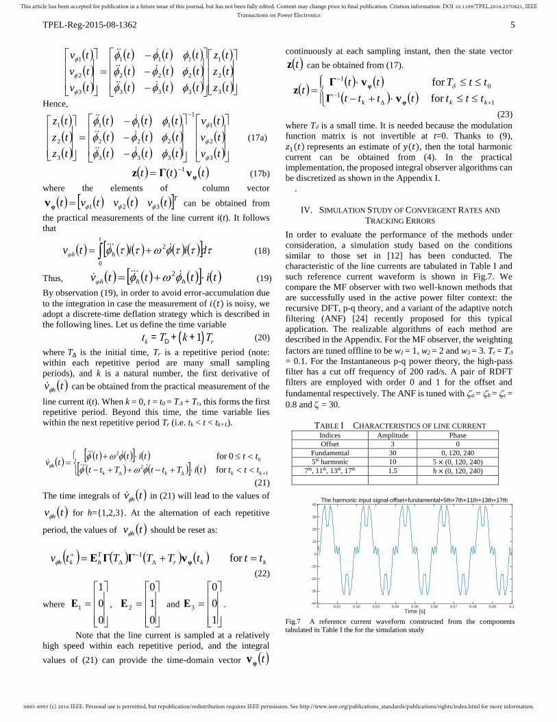
such reference current waveform is shown in Fig.7. We

compare the MF observer with two well-known methods that

are successfully used in the active power filter context: the

recursive DFT, p-q theory, and a variant of the adaptive notch

filtering (ANF) [24] recently proposed for this typical

application. The realizable algorithms of each method are

described in the Appendix. For the MF observer, the weighting

factors are tuned offline to be w1 = 1, w2 = 2 and w3 = 3. Tr = T

= 0.1. For the Instantaneous p-q power theory, the high-pass

filter has a cut off frequency of 200 rad/s. A pair of RDFT

filters are employed with order 0 and 1 for the offset and

fundamental respectively. The ANF is tuned with a = b = c =

0.8 and = 30.

TABLE I CHARACTERISTICS OF LINE CURRENT Indices Amplitude Phase

Offset 3 0

Fundamental 30 0, 120, 240

5th harmonic 10 5 × (0, 120, 240)

7th, 11th, 13th, 17th 1.5 h × (0, 120, 240)

Fig.7 A reference current waveform constructed from the components tabulated in Table I the for the simulation study

Time [s]0 0.01 0.02 0.03 0.04 0.05 0.06 0.07 0.08 0.09 0.1

-40

-30

-20

-10

0

10

20

30

40The harmonic input signal-offset+fundamental+5th+7th+11th+13th+17th



TPEL-Reg-2015-08-1362 6

(8a)

(8b)

(8c)

(8d)

Fig.8 Comparison of the actual harmonics and the extracted harmonics based

on the (a) MF observer, (b) RDFT, (c) Instantaneous p-q power theory and (d) the ANF methods.

Figs. 8(a)-(d) show the actual harmonic current and the

extracted current waveform in the time domain based on the (i)

MF observer, (ii) RDFT, (iii) Instantaneous p-q power theory

and (iv) the ANF methods. For the sake of comparison, the

tracking errors of these four methods are also examined by

subtracting the actual harmonic waveform from the extracted

waveforms. These tracking errors are compared in Fig.9, where

the steady-state errors of the ANF method (which gives the

largest error among the four methods) are used as the error

tolerances (as indicated by the two long dotted lines of ±7 in

Fig.9), the convergence times of these methods to reach the

tolerance region are tabulated in Table II. The p-q theory

method and the MF method have the fastest convergence

performance.

Fig.9 Comparison of tracking error of the four methods under consideration

TABLE II CONVERGENCE TIMES OF THE FOUR METHODS

MF RDFT p-q ANF

Convergence time 10ms 20ms <10ms >20ms

The MF observer takes about 10ms to track the harmonic

waveform and is faster than RDFT and ANF, which require at

least 20ms. Although RDFT offers minimal steady-state error

in a steady-state situation, it is important to note that fast

convergence offers advantage to signal detection applications

in which fast transients and frequency variations are common.

Based on these simulation results, a comparative table with

respect to the steady state error is also constructed as shown in

Table III. The following points can be noted:

1. The results shown in the Table II confirm that the MF

performs the best among all the approaches

2. RDFT is very smooth in steady state; therefore the

relative estimation error decreases as more cycles are

considered.

3. ANF has the worst steady state behavior; therefore the

relative error increases as more cycles are considered.

TABLE III COMPARISON OF RMS VALUES OF THE ESTIMATION ERRORS ON

FIG.9

MF RDFT p-q ANF

0-0.02s (10 cycles) 1.0-pu 2.17-p.u. 1.09-p.u. 1.48-p.u.

0-0.1s (50 cycles) 1.0-pu 2.05-p.u. 1.13-p.u. 2.40-p.u.

V. EXPERIMENTAL VERIFICATION

A third-order MF observer has been implemented to derive

the fundamental and the dc bias current only. The total

harmonic current is then obtained by subtracting dc and

fundamental current components from the line current.

Based on the platform suggested in [12], the total harmonic

currents, settling times, phase errors and overshoots of the

following methods are compared with the practical

measurements.

MF observer

Recursive DFT,

The Instantaneous p-q Theory method

Adaptive Notch Filter (ANF) method [24]

Time [s]0 0.01 0.02 0.03 0.04 0.05 0.06 0.07 0.08 0.09 0.1

-25

-20

-15

-10

-5

0

5

10

15

20

25Reconstructed harmonics by MF observer

actual harmonicsretrieved harmonics

Time [s]0 0.01 0.02 0.03 0.04 0.05 0.06 0.07 0.08 0.09 0.1

-25

-20

-15

-10

-5

0

5

10

15

20

25Reconstructed harmonics by RDFT


Time [s]0 0.01 0.02 0.03 0.04 0.05 0.06 0.07 0.08 0.09 0.1

-25

-20

-15

-10

-5

0

5

10

15

20

25Reconstructed harmonics by p-q theory


Time [s]0 0.01 0.02 0.03 0.04 0.05 0.06 0.07 0.08 0.09 0.1

Fre

qu

ency [

rad

/s]

-25

-20

-15

-10

-5

0

5

10

15

20

25Reconstructed harmonics by ANF


0 0.02 0.04 0.06 0.08 0.1Time [s]

-20

-15

-10

-5

0

5

10

15

20

25The error signal between real harmonics and reconstructed harmonics

ANFp-qRDFTMF



TPEL-Reg-2015-08-1362 7

The algorithms of the 3rd order MF observer are

implemented in a discretized form which is included in

Appendix I. The algorithms of the RDFT and ANF

methods also can be referred to the Appendix I. The

algorithms of the instantaneous p-q theory are well

known and simply follow the block diagrams as shown in

Fig.5. The algorithms under consideration are

implemented in a dSpace DS1006 system. Fig.10 shows

the hardware setup, which includes a programmable

power supply (AMETEK CSW11100), three inductors of

slightly different inductance values, and three resistive

loads. The line currents of the three phase system are

displayed in Fig.11.

Fig.10 Schematic of the three phase converter with resistive loads.

Fig.11 Practical line currents of the three-phase system with a

converter-resistor load.

A Extraction of the fundamental current component

Since the Instantaneous p-q power theory method uses

a high-pass filter to remove the fundamental component in

order to derive the total harmonic current (Fig.5), it is not

included in this comparison because it does not generate the

fundamental current. Only the experimental results of the MF

observer, RDFT and ANF methods are included in this section.

Under a fixed sampling frequency of 10 kHz, the same dSpace

system is used to calculate the fundamental current in real time.

The analogue of this estimated fundamental current is outputted

to a digital storage oscilloscope (DSO-X 3034A). The estimated

fundamental currents of the MF observer, RDFT and ANF

methods are captured and displayed in Figs. 12(a), 12(b) and

12(c), respectively.

In order to observe the deviation of these waveforms

from a pure sinusoidal waveform, let us transform the estimated

sinewave into a unit “circle’’ by picking arbitrarily consecutive

200 samples in one cycle. It is worth noting that a perfect time-

domain sinusoidal function can be represented as an ideal circle

on the 2-D plane. By comparing the trajectory of the measured

current with a perfect circuit, any deviation from the perfect

circle can be observed. One method of measuring the quality of

the extracted fundamental component is the concept of

Circularity [29], which defines the formula for Circularity (C)

2

4

P

AC

(24)

with A and P the area and the perimeter enclosed by of the

circular figure, respectively. Meanwhile, the isoperimetric

theorem indicates that C = 1 only holds for an ideal circle. To

this end, the circularity of each figure is evaluated in the

following way:

1. Divide the shape into circular sectors with radius ri, i =1,2,⋯ ,200 based on the samples.

2. Approximation of the area 𝐴 = ∑1

200

200𝑖=1 𝜋𝑟𝑖

2

3. The perimeter 𝑃 of the curve is approximated by the sum

of the distances between every two adjacent samples.

As such, the vector trajectories of one period of three estimated

fundamental current waveforms are plotted and compared with

a perfect circle in Figs. 13(a), 13(b) and 13(c). It can be

observed that the MF observer method generate the best

fundamental current with the least amount of noise and

distortion. For the sake of completeness, the circularity values

of the MF observer, the RDFT and the ANF have been obtained

and are recorded in Table IV. It can be seen that the curve

generated by MF has the circularity closest to 1 (i.e with the

least absolute deviation from 1.0).

TABLE IV COMPARISON OF CIRCULARITY OF THE EXTRACTED

FUNDAMENTAL COMPONENTS

Circularity

C

Absolute deviation

0.1C

Figure

MF observer 1.0017 0.0017 13(a)

RDFT 0.8925 0.1075 13(b)

ANF 0.8883 0.1117 13(c)

12(a)

12(b)



TPEL-Reg-2015-08-1362 8

12(c)

Fig.12 The estimated fundamental currents obtained from the (a) MF observer,

(b) RDFT and (c) ANF methods.

13(a)

13(b)

13(c)

Fig.13 Comparison of the trajectories of the fundamental currents estimated

by the (a) MF observer, (b) RDFT and (c) ANF methods with the perfect sinusoidal trajectory.

B Detection of the total harmonic current

The second set of evaluation involves all of the four

methods under consideration. This time, the total harmonic

currents estimated by the four methods are captured. Their

harmonic spectra are then plotted and compared with the

harmonic spectrum of the mains current, which is included in

Fig.14 as a reference. Figs. 15(a), 15(b), 15 (c) and 15(d) show

the frequency spectra of the estimated total harmonic currents

obtained from the (a) MF observer, (b) RDFT, (c) Instantaneous

p-q power Theory and (d) the ANF methods, respectively.

Comparing with the spectrum of the measured line current in

Fig.14 and ignoring the part of the spectrum up to about 200 Hz

(to remove the effect of the fundamental current), the spectra of

MF observer, RDFT method and the ANF method are close to

that of the line current.

Fig.14 The measured frequency spectrum of measured line current of Fig.11

15(a)

15(b)

15(c)

15(d)

Fig.15 Measured harmonic spectra of (a) the MF observer, (b) the RDFT, (c)

the Instantaneous p-q power theory and (d) the ANF methods.

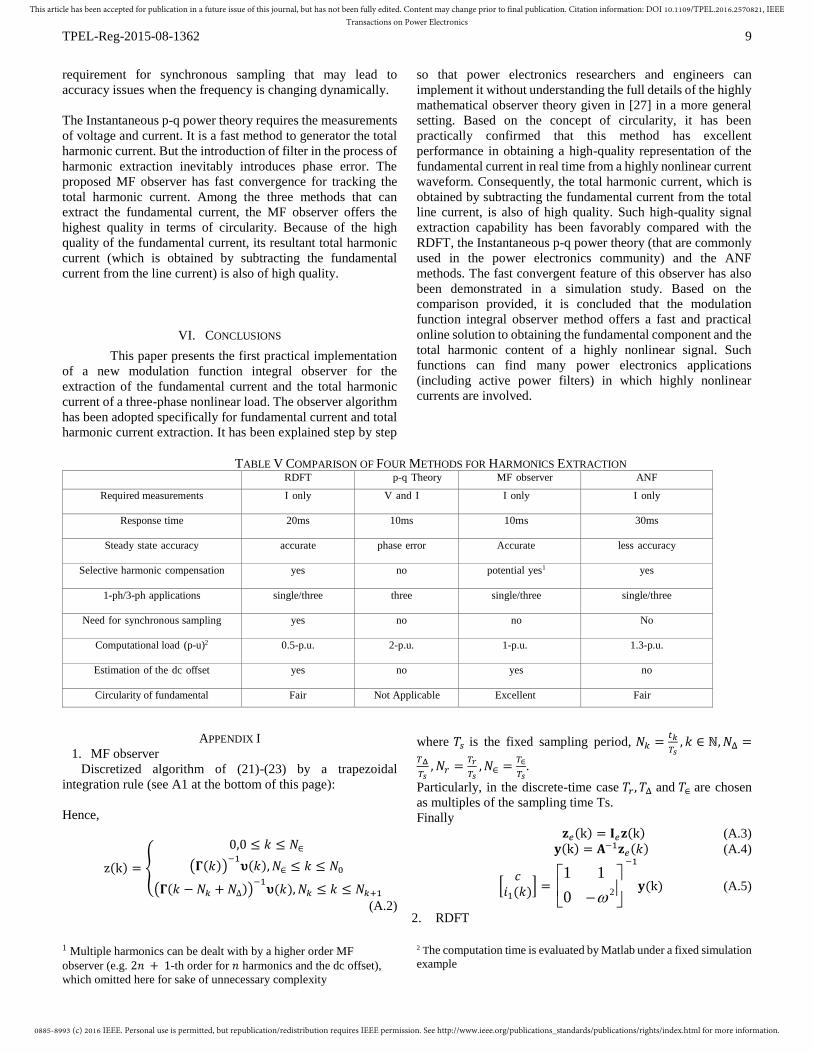
C Overall Comparison

With the results obtained, the performance of the four methods

can be summarized as tabulated in Table V. The RDFT has

generally good performance. The only limitation is its



TPEL-Reg-2015-08-1362 9

requirement for synchronous sampling that may lead to

accuracy issues when the frequency is changing dynamically.

The Instantaneous p-q power theory requires the measurements

of voltage and current. It is a fast method to generator the total

harmonic current. But the introduction of filter in the process of

harmonic extraction inevitably introduces phase error. The

proposed MF observer has fast convergence for tracking the

total harmonic current. Among the three methods that can

extract the fundamental current, the MF observer offers the

highest quality in terms of circularity. Because of the high

quality of the fundamental current, its resultant total harmonic

current (which is obtained by subtracting the fundamental

current from the line current) is also of high quality.

VI. CONCLUSIONS

This paper presents the first practical implementation

of a new modulation function integral observer for the

extraction of the fundamental current and the total harmonic

current of a three-phase nonlinear load. The observer algorithm

has been adopted specifically for fundamental current and total

harmonic current extraction. It has been explained step by step

so that power electronics researchers and engineers can

implement it without understanding the full details of the highly

mathematical observer theory given in [27] in a more general

setting. Based on the concept of circularity, it has been

practically confirmed that this method has excellent

performance in obtaining a high-quality representation of the

fundamental current in real time from a highly nonlinear current

waveform. Consequently, the total harmonic current, which is

obtained by subtracting the fundamental current from the total

line current, is also of high quality. Such high-quality signal

extraction capability has been favorably compared with the

RDFT, the Instantaneous p-q power theory (that are commonly

used in the power electronics community) and the ANF

methods. The fast convergent feature of this observer has also

been demonstrated in a simulation study. Based on the

comparison provided, it is concluded that the modulation

function integral observer method offers a fast and practical

online solution to obtaining the fundamental component and the

total harmonic content of a highly nonlinear signal. Such

functions can find many power electronics applications

(including active power filters) in which highly nonlinear

currents are involved.

TABLE V COMPARISON OF FOUR METHODS FOR HARMONICS EXTRACTION RDFT p-q Theory MF observer ANF

Required measurements I only

V and I I only

I only

Response time 20ms

10ms

10ms

30ms

Steady state accuracy accurate

phase error Accurate

less accuracy

Selective harmonic compensation yes

no

potential yes1 yes

1-ph/3-ph applications single/three three

single/three single/three

Need for synchronous sampling yes

no

no

No

Computational load (p-u)2 0.5-p.u.

2-p.u.

1-p.u.

1.3-p.u.

Estimation of the dc offset yes

no

yes

no

Circularity of fundamental Fair Not Applicable Excellent Fair

APPENDIX I

1. MF observer

Discretized algorithm of (21)-(23) by a trapezoidal

integration rule (see A1 at the bottom of this page):

Hence,

z(k) = {

0,0 ≤ 𝑘 ≤ 𝑁∈

(𝚪(𝑘))−1𝛖(𝑘), 𝑁∈ ≤ 𝑘 ≤ 𝑁0

(𝚪(𝑘 − 𝑁𝑘 + 𝑁∆))−1𝛖(𝑘), 𝑁𝑘 ≤ 𝑘 ≤ 𝑁𝑘+1

(A.2)

1 Multiple harmonics can be dealt with by a higher order MF

observer (e.g. 2𝑛 + 1-th order for 𝑛 harmonics and the dc offset),

which omitted here for sake of unnecessary complexity

where 𝑇𝑠 is the fixed sampling period, 𝑁𝑘 =𝑡𝑘

𝑇𝑠, 𝑘 ∈ ℕ,𝑁Δ =

𝑇Δ

𝑇𝑠, 𝑁𝑟 =

𝑇𝑟

𝑇𝑠, 𝑁∈ =

𝑇∈

𝑇𝑠.

Particularly, in the discrete-time case 𝑇𝑟 , 𝑇Δ and 𝑇∈ are chosen

as multiples of the sampling time Ts.

Finally

𝐳𝑒(k) = 𝚰𝑒𝐳(k) (A.3)

𝐲(k) = 𝐀−1𝐳𝑒(𝑘) (A.4)

[𝑐

𝑖1(𝑘)] =

20

11

−1

𝐲(k) (A.5)

2. RDFT

2 The computation time is evaluated by Matlab under a fixed simulation

example



TPEL-Reg-2015-08-1362 10

It has been show that the RDFT is very convenient in

extracting a specific harmonic component from a given

current 𝑖(𝑡) by the following recursive algorithm (𝑗 is the

order of the desired harmonic

ℎ𝑗(𝑘) =2

𝑁(𝑖(𝑘) − 𝑖(𝑘 − 𝑁)) +𝑊𝑗ℎ𝑗(−1) (𝐴. 6)

which is driven by its equivalent transfer function 𝐺𝑗(𝑧)

between the input 𝑖(𝑧) and the extracted harmonic signal

ℎ𝑗(𝑧), :

𝐺𝑗(𝑧) =ℎ𝑗(𝑧)

𝑖(𝑧)=1

𝑁

1 − 𝑧−𝑁

1 −𝑊𝑗𝑧−1 (𝐴. 7)

3. p-q theory

The reader is referred to Figure 5 for the overall scheme.

4. Adaptive notch filtering (ANF)

Herein, a recent ANF [24] is picked for the sake of

comparison and is reviewed in the following equations (the

single-phase structure):

{

ℎ𝑗(𝑡) = −𝑗

2𝜃(𝑡)2ℎ𝑗(𝑡) + 2ζ𝑗𝜃(𝑡)𝑒(𝑡)

𝑒(𝑡) = 𝑖(𝑡) −∑ℎ𝑙

𝑛

𝑙=1

��(𝑡) = −𝛾𝜃(𝑡)ℎ1(𝑡)𝑒(𝑡)

(A. 8)

where 𝑖(𝑡) represents the current signal from each phase

respectively, 𝜃 is the estimate of the fundamental frequency

𝜔, 𝑗 = 1, 2,⋯ , , 𝑛 is the order of the selected harmonic, ζ𝑗 , 𝛾

are all positive adjustable parameters balancing the converging

speed and accuracy, 𝑙 is the sequence of the harmonic that is

estimated. The continuous-time algorithm can simply

discretized by Euler or trapezoidal rules for digital

implementation.

APPENDIX II

A nominal state observer (i.e., Luenberger Observer) is

applicable for the linear system (7). However, only asymptotic

convergence is guaranteed (i.e., the estimated state z(t) →z(t), when t → ∞), because of the initial error driven by the

unknown initial condition. In order to circumvent this

restriction and to propose an observer that can converge within

an arbitrary small finite time, we annihilate the influence of the

unknown initial condition by exploiting an integral operator

(see (18)) with respect to the designed modulation function.

The next Lemma introduced in [27] is instrumental for the

following description.

Lemma 1 (Modulated signal’s derivative): Consider a signal

𝑥(𝑡), 𝑡 ≥ 0 that admits a 𝑖-th order derivative, and a i-th order

differentiable modulation function 𝑉𝜙𝑥(𝑡), 𝑡 ≥ 0 . It holds that:

[𝑉𝜙𝑥(𝑖)](𝑡) = ∑(−1)𝑖−𝑗−1

𝑖−1

𝑗=0

𝑥(𝑗)(𝑡)𝜙(𝑖−𝑗−1)(𝑡)

+∑(−1)𝑖−𝑗𝑖−1

𝑗=0

𝑥(𝑗)(0)𝜙(𝑖−𝑗−1)(0)

+ (−1)𝑖 [𝑉𝜙𝑖𝑥] (𝑡)

where we let the 𝑑𝑖

𝑑𝑡𝑖𝑥(𝑡) ≜ 𝑥(𝑖)(𝑡) for the sake of brevity and

we define the modulation operator by

[𝑉𝜙𝑥](𝑡) ≜ ∫ 𝜙(𝜏)𝑥(𝜏)𝑑𝜏𝑡

0

.

The above Lemma motivates us to eliminate the unknown

initial conditions 𝑥(0),𝑑1

𝑑𝑡1𝑥(0),

𝑑2

𝑑𝑡2𝑥(0),⋯ by choosing a

modulation function 𝜙(𝑡), such that 𝑑𝑛

𝑑𝑡𝑛𝜙(0) = 0 (𝐴9)

Thanks to (A9), we design the following modulating function

𝜙ℎ =𝑤ℎ𝑡

2𝑛−ℎ

(2𝑛 − ℎ)! , ℎ = {1,2,⋯ 𝑛}

{

ν𝜙ℎ(𝑘 + 1) = ν𝜙ℎ(𝑘) +

1

2𝑇𝑠 ((𝜙ℎ(𝑘 + 1) + 𝜔

2𝜙ℎ(𝑘 + 1)) 𝑖(𝑘 + 1) + (𝜙ℎ(𝑘) + 𝜔2𝜙ℎ(𝑘)) 𝑖(𝑘)) , 0 ≤ 𝑘 < 𝑁0

ν𝜙ℎ(𝑘 + 1) = ν𝜙ℎ(𝑘) +1

2𝑇𝑠 (

(𝜙ℎ(𝑘 + 1 − 𝑁𝑘 +𝑁Δ) + 𝜔2𝜙ℎ(𝑘 + 1 − 𝑁𝑘 + 𝑁Δ)) 𝑖(𝑘 + 1) +

(𝜙ℎ(𝑘 − 𝑁𝑘 +𝑁Δ) + 𝜔2𝜙ℎ(𝑘 − 𝑁𝑘 + 𝑁Δ)) 𝑖(𝑘)

) , 𝑁𝑘 < 𝑘 < 𝑁𝑘+1

ν𝜙ℎ(𝑁𝑘+) = 𝐸ℎ

𝑇𝚪(𝑁Δ)𝚪(𝑁r + 𝑁Δ)−1𝛎(𝑁𝑘), 𝑘 = 𝑁𝑘 . (A1)



TPEL-Reg-2015-08-1362 11

where the index ℎ allows a set of modulation functions in this

form distinguished by different parameter 𝑤ℎ and order ℎ .

Admittedly, the choice of the modulation function satisfying

(A9) is not unique. For this application paper, we only show

this typical function as a simple example. Although the

modulation function plays an important role in this

methodology, the selection does not vary from application to

application; the modulation functions satisfying (A9) are

applicable for the state estimation problem of any linear system

in which the harmonic model can be embedded.

Acknowledgement:

This work was partially supported by the HK Research Grant

Council under the Theme-based Research Fund T23-701/14-N.

REFERENCES

[1] A. Segura and P. Sanchez, “Experimental measurement of non-

characteristic harmonic power generated by thyristor pulse-controlled ac/dc three phase converters,” in Proceedings of the IEEE International

Symposium on Industrial Electronics, 1996, pp. 549–554.

[2] A. Phadke and J. Harlow, “Generation of abnormal harmonics in high-voltage ac-dc power systems,” IEEE Transactions on Power Apparatus

and Systems, vol. 87, no. 3, pp. 873–883, 1968.

[3] K. Patil and W. Gandhare, “Effects of harmonics in distribution systems on temperature rise and life of XLPE power cables,” in International

Conference on Power and Energy Systems (ICPS), 2011, pp. 1–6.

[4] J. D. H. Harold A. Gauper and A. McQuarrie, “Generation of abnormal harmonics in high-voltage ac-dc power systems,” IEEE Spectrum, vol.

8, no. 10, pp. 32–43, 1971.

[5] M. Lowenstein, “Improving power factor in the presence of harmonics using low voltage tuned filters,” in Conference Record of the 1990 IEEE

Industry Applications Society Annual Meeting, 1990, pp. 1767–1773.

[6] H. Akagi, “New trends in active filters for power conditioning,” IEEE Transactions on Industry Applications, vol. 32, no. 6, pp.1312–1322,

1996.

[7] A. C. Bhim Singh, K. Al-Haddad and, “A review of active filters for power quality improvement,” IEEE Transactions on Industrial

Electronics, vol. 46, no. 5, pp. 960–971, 1999.

[8] H. Akagi, “Active harmonic filters,” in Proc. of the IEEE, vol. 93, no. 12, 2005, pp. 2128–2141.

[9] H. Akagi, “Trends in active power line conditioners,” IEEE Transactions

on Power Electronics, vol. 9, no. 3, pp. 263–268, 1994. [10] F. Z. Peng, “Application issues of active power filters,” IEEE Industry

Applications Magazine, vol. 4, no. 5, pp. 21–30, 1998.

[11] “Advanced Activer Power Filters: A flexible and adaptive solution for central or de-central harmonic mitigation”, [Online]. Available:

http://www.danfoss.com/NR/rdonlyres/87CF6FEA-CA08-4518-AE36-

8534104DFA38/0/VLTAdvancedActiveFilterFactsheetMP012A023.pdf

[12] L. Asiminoaei, F. Blaabjerg, and S. Hansen, “Evaluation of harmonic

detection methods for active power filter applications,” in Applied Power Electronics Conference and Exposition, 2005. APEC 2005. Twentieth

Annual IEEE, 2005, pp. 635–641.

[13] D. Kucherenko and P. Safronov, “A comparison of time domain harmonic detection methods for compensating currents of shunt active

power filter,” in IEEE International Conference on Intelligent Energy

and Power Systems (IEPS), no. 12, 2014, pp. 40–45. [14] B. McGrath, D. Holmes, and J. Galloway, “Power converter line

synchronization using a discrete fourier transform (dft) based on a variable sample rate,” IEEE Trans. on Power Electron., vol. 20, no. 4, pp.

877–884, 2005.

[15] S. Gonzalez, R. Garcia-Retegui, and M. Benedetti, “Harmonic computation technique suitable for active power filters,” IEEE Trans. on

Ind. Electron., vol. 54, no. 5, pp. 2791–2796, 2007.

[16] E. Jacobsen and R. Lyons, “The sliding DFT,” IEEE Signal Process. Mag., vol. 20, no. 2, pp. 74–80, 2003.

[17] E. Jacobsen and R. Lyons, “An update to the sliding DFT,” IEEE Signal

Process. Mag., vol. 21, no. 1, pp. 110–111, 2004.

[18] A. A. Girgis, W. B. Chang, and E. B. Makram, “A digital recursive

measurement scheme for on-line tracking of power system harmonics,” IEEE Trans. on Power Delivery, vol. 6, no. 3, pp. 1153–1160, 1991.

[19] X. Yuan, W. Merk, H. Stemmler, and J. Allmeling, “Stationary-frame

generalized integrators for current control of active power filters with zero steady-state error for current harmonics of concern under

unbalanced and distorted operating conditions,” IEEE Trans. Ind. Appl.,

vol. 38, no. 2, pp. 523–532, 2002. [20] P. Rodriguez, A. Luna, I. Candela, R. Mujal, R. Teodorescu, and F.

Blaabjerg, “Multiresonant frequency-locked loop for grid

synchronization of power converters under distorted grid conditions,” IEEE Trans. Ind. Electron., vol. 58, no. 1, pp. 127–138, 2011.

[21] Y. F. Wang and Y. W. Li, “Three-phase cascaded delayed signal

cancellation pll for fast selective harmonic detection,” IEEE Trans. on Ind. Electron., vol. 60, no. 4, pp. 1452–1463, 2013.

[22] M. Karimi-Ghartemani and M. R. Iravani, “Measurement of

harmonics/inter-harmonics of time-varying frequencies,” IEEE Trans. on Power Delivery, vol. 20, no. 1, pp. 23–31, 2005.

[23] M. Mojiri, M. Karimi-Ghartemani, and A. Bakhshai, “Time-domain

signal analysis using adaptive notch filter,” IEEE Trans. on Signal Processing, vol. 55, no. 1, pp. 85–93, 2007.

[24] D. Yazdani, A. Bakhshai, G. Joos, and M. Mojiri, “A real-time three-

phase selective-harmonic-extraction approach for grid-connected converters,” IEEE Transactions on Industrial Electronics, vol. 56, no. 10,

pp. 4097–4106, 2009.

[25] M. Mojiri, M. Karimi-Ghartemani, and A. Bakhshai, “Processing of harmonics and inter-harmonics using an adaptive notch filter,” IEEE

Trans. on Power Delivery, vol. 25, no. 2, pp. 534–542, 2010. [26] V. M. Moreno, M. Liserre, A. Pigazo, and A. D. Aquila, “A comparative

analysis of real-time algorithms for power signal decomposition in

multiple synchronous reference frames,” IEEE Trans. on Power Electron., vol. 22, no. 4, pp. 1280–1289, 2007.

[27] G. Pin, B. Chen, and T. Parisini, “The modulation integral observer for

linear continuous-time systems,” in Proc. of the IEEE European Control Conference, Linz, 2015.

[28] H. Kim and H. Akagi, “The instantaneous power theory based on

mapping matrices in three-phase four-wire systems,” in IEEE Proc. of Power Conversion Conference, 1997, pp. 361–366.

[29] V. Blasjo, “The Evolution of the Isoperimetric Problem,” Amer. Math.

Monthly 112: 526–566.

a fast-convergent modulation integral observer for online ... · discrete kalman filtering (dkf)...

Documents