arX

iv:1

605.

0143

5v2

[cs

.DB

] 9

May

201

6

A Fast Lightweight Time-Series Store for IoT Data

Daniel G. WaddingtonSamsung Research America

Mountain View, CA

daniel.waddington@acm.org

Changhui LinSamsung Research America

Mountain View, CA

changhui.lin@samsung.com

ABSTRACTWith the advent of the Internet-of-Things (IoT), handlinglarge volumes of time-series data has become a growing con-cern. Data, generated from millions of Internet-connectedsensors, will drive new IoT applications and services. A keyrequirement is the ability to aggregate, preprocess, index,store and analyze data with minimal latency so that time-to-insight can be reduced. In the future, we expect real-timedata collection and analysis to be performed both on smalldevices (e.g., in hubs and appliances) as well in server-basedinfrastructure. The ability to localize sensitive data to thehome, and thus preserve privacy, is a key driver for small-device deployment.

In this paper, we present an efficient architecture for time-series data management that provides a high data inges-tion rate, while still being sufficiently lightweight that itcan be deployed in embedded environments or small vir-tual machines. Our solution strives to minimize overheadand explores what can be done without complex indexingschemes that typically, for performance reasons, must beheld in main memory. We combine a simple in-memory hi-erarchical index, log-structured store and in-flight sort, witha high-performance data pipeline architecture that is opti-mized for multicore platforms. We show that our solution isable to handle streaming insertions at over 4 million recordsper second (on a single x86 server) while still retaining SQLquery performance better than or comparable to existingRDBMS.

1. INTRODUCTIONBy 2020, analysts predict that there will be over 25 billion

connected devices in the Internet-of-Things (IoT). Together,these devices will generate unprecedented volumes of datathat must, in order to create value, be efficiently indexed,stored, queried and analyzed. A single aspect that ties allof this data together is that it is time-series. Time is eitherevident as an explicit dimension in the data (e.g., a sensorgenerated time-stamp) or implicit by the time at which a

data sample reaches an aggregation node (e.g., a hub orserver).

Existing databases and storage systems predominantlyhandle time-series data no differently from other data. Theredoes exist a notion of time-series database, some that arebased on RDBMS and some that based on NoSQL type ar-chitectures. While APIs and data types may be providedspecifically for time, the underlying storage and indexingmechanisms are no different. As a consequence of generality,existing RDBMS solutions are typically limited to ingressstreams of 200-300K RPS on a single commodity server and25-30K RPS on an embedded platform. Their performanceis limited primarily because of the complexity introduced byindexing with B+-trees [14] or LSM trees [18] as well as themaintenance of locks and state for transactional processing.

However, a key strength of RDBMS solutions is their abil-ity to support advanced queries through SQL support [15].SQL provides a powerful language for performing arbitraryqueries that require filtering (selection), manipulation (e.g.,data conversion), projection (e.g., aggregation), and joins.SQL also provides a standardized and industry accepted in-terface to which analytic solutions (e.g., Apache Spark [20],Tableau [9], SAS [8], SAP [7]) and applications can be easilyintegrated.

We believe that this type of complex query is a key en-abler for future IoT applications that derive value by cre-ating insight from data. By digitally enabling a productthrough sensor augmentation, massive volumes of data canbe collected about operation, wearing and environmentalconditions. Combining this with analytics that can quicklyslice-and-dice the data, enables new hybrid product-servicemodels to be realized (e.g., preventative maintenance, en-ergy optimization).

While most database solutions provide SQL access to data,they inherently cannot support continuous ingest of large-volumes of streaming data. Those solutions that do providehigher ingest rate capabilities typically make extensive useof main memory to hold indexing information.

The focus of this work is the development of a lightweightand memory-efficient architecture that supports an order-of-magnitude higher ingest rate over existing RDBMS andtime-series database solutions. We do this while still pro-viding both the flexibility and power of SQL, and a minimalrun-time memory overhead so as to be suitable for deploy-ment in embedded or resource-limited environments.

Our solution, herein termed Lightweight Time-Series Store(LTSS), is domain-specific in that it is designed to leveragethe characteristics of time-series data in an IoT application

1

context.Specifically, LTSS is designed with the following assump-

tions in mind:

i Data is highly-ordered - Time advances and thus datais inherently in order. Network routing and impreciseclock synchronization (i.e., inability to have a true globalclock) can cause out-of-order data, but this is typicallylimited to a finite time window (samples outside of sucha window can be considered invalid and not useful).

ii Data is immutable - Each data element represents a sam-ple in time that may or may not be subsumed by a sub-sequent sample, but in itself represents an unchangeablehistory. Applications generally summarize and aggre-gate data to create useful insight.

iii Both epoch and calendar-based reasoning are necessary

for analytics - While epoch-based time are useful, alonethey are insufficient. Many analyses require reasoningin terms of human-understandable concepts (e.g., hours,days, months). For example, queries such as “Is thecurrent value the highest for the month?” are typical.

iv Data can be lost - Most data is collected over unreli-able wireless network links and through congested IProuters. Sensor-based data sources do not, in the mostpart, have the ability to perform re-transmission due tolimited energy and memory capacities. IoT applicationsare predominantly resilient to data loss.

1.1 Deployment RequirementsOur architecture focuses on indexing and query at the

ingestion node. The ingestion node is the first “point ofcontact” for data being collected from sensors distributedacross a network. Data is received either directly from thesensor (e.g., where a sensor has direct Internet connectivity)or from a hub (e.g., that aggregates across multiple non-IPsensors). Its role is to receive streaming data, which is thenpreprocessed, stored and indexed according to one or moretime fields, and made accessible through read-only queryinterfaces.

The ingestion node is responsible for the management of“fresh” data. It has limited storage resources and can onlystore data for a given period of time. Old data is eitheroff-loaded to cold-storage (e.g., in the cloud) or erased.

An ingestion node implementation may take multiple formsdepending on the deployment context. For example, in thehome it may be realized in one or more hub devices or em-bedded into existing consumer electronics (e.g., a SmartTV).At the network edge, the ingestion node may be deployedon commodity x86 servers or cloud infrastructure. We donot envisage the deployment of ingestion nodes at the cloudback-end due to the cost of back-hauling data.

For our work we are particularly focused on in-home andedge deployments. We define the following requirements ac-cordingly:

i. High-Volume Data Rates - Support for continuous ag-gregation and summarization of large volumes of stream-ing data resulting from an increasing number of de-ployed sensors with higher data generation rates (i.e.,increased sampling frequencies).

ii. Flexible Memory Model - Tailorability of main memoryoverhead according to available resources. Less than32MB minimum memory footprint in an embedded en-vironment.

iii. Low-Latency for Real-time Applications - Freshness ofdata (i.e., the time between the data being received andit being accessible to queries) should be in the orderof 200-400ms (latency deemed necessary for interactiveapplications).

iv. SQL-based Query Interface - The system should supportSQL in order to easily integrate with existing platformsand applications while also providing query flexibilityto support complex operations and joins across multipledata sources.

v. Data Aging and Resource Re-cycling - Data should bestored using a fixed set of resources (disk,memory). Ag-ing data should override new data as resources are ex-hausted.

1.2 OutlineThe rest of this paper is organized as follows. Section 2

presents some background and related work, and positionsour own work in the field of time-series/streaming databases.In Section 3, we present our architecture and provide detailson how data from continuous streams is ordered, indexedand stored, and how it is integrated with an SQL front-end.Section 4 describes details around the prototype implemen-tation. Next, Section 5, presents our evaluation based onthree real-world data sets with representative queries andalso discuss our testing methodology. Finally, in Section 6we offer our conclusions.

2. RELATED WORKThere currently exists a broad range of time-series databases,

both commercially and as open source. These databasesprovide additional capabilities that are specific to stream-ing data ingest and time-oriented queries. With the adventof IoT, these databases vendors and developers are toutingsupport for store and analysis of large volumes of sensordata. The specific features of each are also varied. Table 1lists some of the more popular time-series database solutionsand highlights their different feature sets.

The work in this paper focuses on the following key capa-bilities:

• High ingest rates

• Support for an SQL interface

• Local write-append data storage

Of the technologies listed in Table 1, PipelineDB, ParStream,IBM Informix and InfiniFlux meet this criteria and are thusmost relevant to our work. However, they are not designedwith embedded and other resource constrained environmentsin mind.

Pipeline DB [5], an open source project primarily devel-oped by Usman Masood, is aimed at performing SQL querieson streaming data. Specifically, it is designed to excel atSQL queries that reduce the cardinality of streaming datasets through aggregation and summarization. Raw data isdiscarded once it has been read by the continuous queries

2

Name Impl.Lang.

Interface SQLAd-hocQueries

Cont.Queries

License DataStore

Data Struct. Advertised IngestRate (Per-Node)

Akumuli C++ JSON N N Open Local Log 200K RPS

Bolt C# C# API N N Proprietary Distributed LSM 100K RPS

Druid Java HTTP/REST N Y Open Distributed Columnar 10K RPS

IBM Informix - REST/SQL/JSON Y N Commercial Local unknown 420K RPS

InfiniFlux C++ SQL Y Y Commercial Local Columnar 2M RPS

InfluxDB Java HTTP/REST Partial Y Open Local LSM 100-150K RPS

OpenTSDB Java HTTP/CLI N N Open Distributed HBase/Cassandra 100K RPS

ParStream C++ JDBC/SQL Y N Commercial Distributed Columnar 500K RPS

PipelineDB C++ SQL Y Y Open Local B-tree 500K RPS

Prometheus Go HTTP/JSON Y N Open Local LSM unknown

LTSS C++ SQL Y Partial Proprietary Local Log 4M+ RPS

Table 1: Popular Time-Series Databases.

that need to read it. Pipeline DB provides full SQL sup-port and provides additional constructs to support querieson sliding windows and continuous materialization. As withour own philosophy, Pipeline DB aims to eliminate an ex-plicit extract-transform-load stage from the data analyticspipeline. The system is based on, and fully compatible with,PostgreSQL 9.4, and therefore uses B-tree/hash based in-dexing. Pipeline DB uses PostgreSQL’s INSERT and COPYconstructs for writing data. In the long term, the PipelineDB team hope to factor out the solution as a PostgreSQLextension, suggesting that they do not plan to change thestorage internals.

ParStream [4, 10], recently acquired by Cisco, is a broaderanalytics platform aimed at IoT (originally ParStream wastouted as a real-time database for big data analytics). Theirkey differentiators are fast ingest, edge analytics and theability to create real-time insights through concurrent fastqueries. The ParStream architecture leverages both in-memoryprocessing (for indices and data caching) and disk-basedstorage. The system has been explicitly designed to ex-ploit multicore architectures by the use of parallel process-ing. The crux of the ParStream DB indexing is their HighPerformance Compressed Index (HPCI), which is currentlyin patent application [16]. HPCI is a compressed bitmapindex on which queries can be directly executed. This bothreduces the time to scan records and the memory footprintfor the index. Unlike LTSS, the ParStream architecture sep-arates out Import and Query Nodes. This allows them toalter the ratio of query and ingest resources. Import Nodes,basically perform an extract-transform-load stage, convertincoming data into an internal data partition format. It ispossible to transform data based on SQL statements exe-cuted in the Import Nodes. ParStream provides SQL overJDBC/OBDC, as well as a C++ interface. The system alsosupports cluster-based deployment and replication, whichLTSS does not.

InfiniFlux [3] is another commercial time-series databasesolution. It is a columnar DBMS tailored to processingtime-series “machine data” at high ingest speeds (millionsof records per second on a single node). Like ParStream,InfiniFlux uses an in-memory bitmap based index to man-age the data. Columns are set up for each potential valueand bit vectors used to indicate the value for a given row.This provides significant compression for data sources whose

value ranges are limited (e.g., sensor data ranging for 0-255). InfiniFlux is designed to achieve maximum analyticalperformance by storing records in a hybrid arrangement ofcolumn-oriented coupled with time-partitioned. InfiniFluxadvertises an ingest rate of around 2M records per second.

Finally, IBM Informix, a broader commercial RDBMSsuite, provides a specific solution for time series data knownas Informix TimeSeries [2]. At the core of ITS is the Dat-aBlade extensibility framework, which allows the user tocustomize and enhance types and functions in the databasesystem. In essence, the TimeSeries enhancements provideadditional data types and compressed storage schemes. Sim-ilar to the LTSS composite time type (see Section 3.1), In-formix TimeSeries provides a CalendarPattern data typethat allows intervals based on calendar fields (e.g., second,minute, hour) to be easily defined. It also provides othertime-specific data types for regular and irregular time-series(grouping together rows ordered by time stamp). Time-series data can be stored in rows (when less than 1500 bytes)or in containers that store the data outside of the databasetables. These, like LTSS, are contiguous append-only logs.

All of these solutions are primarily designed with serverdeployment in mind. They intentionally leverage a com-bination of storage and (large) main memory to acceleratesystem performance. LTSS on the other hand, makes mini-mal use of main memory, but is designed to exploit randomaccess performance of new non-volatile RAM storage tech-nologies.

3. ARCHITECTUREThe LTSS system is designed around a component-based

data processing architecture that allows flexible configura-tion of real-time compute and storage.

Ingestion Pipeline (write-only)

Time

Ordering

Record

StorageChannel

Source

Time

Conversion

Database

Integration

(read-only)

NIC

Actor

Figure 1: LTSS High-Level View

The LTSS ingestion pipeline has four main components(see Figure 1):

3

• Channel Source - The Channel Source component hasan active thread that consumes data from the NICactor (via a data plane channel). It simply takes eachrecord and passes it on through a down-stream call.

• Time Conversion - Conventional UNIX epoch (or higherprecision) time stamps are converted to a concise cal-endar based “composite” time (see Section 3.1). Thisallows the system to accelerate data selection basedon calendar patterns (e.g., every first Tuesday in themonth). Note that this conversion is performed duringthe data ingest.

• Time Ordering - The Time Ordering component en-sures that ingress packets are ordered according totime. Out of order records may arise from lack ofglobal clock synchronization, Internet routing, and OSscheduling. Records are ordered through an insertionsort.

• Record Store - The final stage of the ingestion pipelineis the Record Store. The Record Store provides an in-terface for write-append, time-ordered storage of records.Data is stored as a log with in-memory metadata toaccelerate look up. We do not currently do any com-pression on the stored data.

The query side (read-only) runs as a separate process thatinteracts with the pipeline through shared memory.

3.1 Composite Time RepresentationA calendar-based, composite time type (ctime t), with

microsecond precision, is used to represent indexed timecolumns (this sub-second precision is necessary for IoT ap-plications). The ctime t type uses a compact bit field rep-resentation totaling only 8 bytes (see below). This is consid-erably more memory efficient than the POSIX tm structurethat requires 36 bytes. Calendar-based field extraction ismore efficient with composite time than using a basic timestamp.

unsigned usec: 20; // range 0-999999unsigned sec: 6; // 0-59unsigned min: 6; // 0-59unsigned hour: 5; // 0-23unsigned wday: 3; // 0-6unsigned day: 5; // 0-31unsigned month: 4; // 0-11unsigned year: 5; // 2000 up to 2031unsigned timezone: 5; // 0-23unsigned pm: 1; // 0-1unsigned dls: 1; // 0-1unsigned reserved: 3;

All time columns, on which query constraints can be ex-pressed, are represented with the ctime t type. Standardconverters, that are executed in the pipeline, are imple-mented for epoch and ISO 8601 string-based time formats.Records stored in the LTSS must have at least one compos-ite time field. The current implementation only supportsconstraints on one instance of composite time.

3.2 In-flight Record OrderingIngress records are allocated to “quantum buckets” (see

Figure 2). Each bucket represents a relative time window.The target bucket for a given record is simply calculatedby rounding down the record’s time stamp (epoch or com-posite). Buckets are created on-demand providing that no

Quantum Buckets Insertion Sort Record Store

Async Sorting Thread

ingress packets FIFO LF Queue

Figure 2: Time Ordering Architecture

Year

Month

Day

WDay

Min

Second

storage absolute o!sets

interval tree

Figure 3: Record Store Metadata

future bucket (i.e. with a greater time stamp) has alreadybeen created and closed (a record attempting to create sucha bucket is considered “delinquent” and is dropped). Buck-ets are arranged in an ordered queue and expired from thetail according to time. The duration of the quantum, andthus the length of the wait in the queue before sorting andclosing, implicitly defines the freshness of data. This at-tribute is configurable.

When the Time Ordering component expires a bucket, itasynchronously passes the set of records for the quantumto a sorting thread. This performs an insertion sort on therecords before passing them to the Record Store. We usean insertion sort because of its good performance in sortingnearly ordered lists with typically a small number of placesan element can be out of order [12].

3.3 In-Memory Directory IndexThe Record Store uses a shared memory directory-style

index to accelerate look up performance. A dynamic list ofabsolute byte offsets is maintained for each composite timefield down to second granularity (see Figure 3). Each listmaintains offsets to the starting point for every instance ofthe given field. For example, the Year list contains a singleoffset for each year the data covers. The Month list containsan offset for each month covered and so on and so forth.Interval trees [13] are used to augment the field lists so thatthe location of the appropriate offset can be quickly made.This is especially beneficial for least-significant fields suchas minutes and seconds.

Query constraints are applied starting from the most-significant field (e.g., Year = 2015). Once the offset is lo-cated for the appropriate year (more than one year may ex-ist), it is used to quickly narrow on the next constraint (e.g.,Month = Mar). That is, the offset for the matching 2015year is subsequently used in matching on the interval treeto find the first matching month within 2015 (see Figure 4).Sub-second constraints are realized through an exponentialsearch (i.e., binary chop).

A persistent version of the in-memory metadata is main-tained for fast recovery. The memory footprint for this indexis typically in the order of tens of megabytes.

4

Constraint: 2015, Mar

2014

2015

MAYJUNJULAUGSEPOCTNOVDECJANFEBMARAPRMAY

Log

ica

l o!

set

axi

s

Figure 4: Metadata Offset.

3.4 Retrieval APIsThe LTSS system separates ingress processing and data

retrieval across separate processes. Data access is read only;the system does not support insertion or deletion. Recordsare implicitly deleted/overwritten when storage capacity isexhausted (see Section 4.8 on rolling-around).

Queries can be made programmatically through the RecordReader interface, which provides a standard iterator patternC++ API. Data can also be accessed through SQL via theSQLite3 virtual table mechanism [11]. The virtual table im-plementation backs onto the IRecordReader interface. Thispresents the data through a table abstraction in which SQLexpressions can be applied.

4. IMPLEMENTATION DETAILS

4.1 Component ModelThe fundamental building blocks of data pipelines are ac-

tors and components. Actors are memory-protected pro-cesses that exchange control messages through shared mem-ory. They have at least one thread and typically createnew threads for each client connection. Messages, based onGoogle Protobuf [6], are typed and exchanged by either localIPC or network RPC. Furthermore, actor messages are ei-ther synchronous or asynchronous (the latter being typical ofa stricter actor model). Actors are composed of components,which are in-process loadable entities that provide typed in-terfaces and receptacles that can be dynamically inspectedand bound (much like Microsoft’s COM architecture [19]).Components do not impose any threading model.

4.2 Zero-Copy Data PlaneData belonging to flows are exchanged through asynchronous

lock-free FIFO queues. Units of data, which we term records,are exchanged between processes in shared memory and arethus zero-copy. Record memory is allocated (producer side)and freed (consumer side) from a thread-safe slab allocatorthat uses a circular lock-free queue to track slab elements.Both the slab allocator queue and the exchange queue can beconfigured with SPSC (Single-Producer, Single Consumer)or MPMC (Multi-Producer, Multi-Consumer) queues de-pending on the requirements of the deployment scenario.

NUMA-Allocated

Memory Slab

Lock-free Circular Queue

(SPSC, MPMC)

Memory Allocator

Lock-free Bounded FIFO (SPSC, MPMC)Producer

Threads

Consumer

Threads

alloc free

Figure 5: Zero-copy IPC

4.3 NIC ActorThe prototype LTSS system operates on UDP/IP (version

4) data packets and makes no assumption about aggrega-tion. IP provides global connectivity while UDP provides asimple protocol for “fire-and-forget” datagram transmission.The current prototype does not use packet authentication orencryption even though this would be likely in a real-worlddeployment. In our experimentation, our sensor packets aresmall (< 512 bytes).

4.4 User-Level Network StackTo maximize network performance, the server-based im-

plementation adopts an exokernel design (see Figure 6) thatallows the Network Interface Card (NIC) device driver tofully operate in user-space [1]. In addition to the NIC driver,a lightweight UDP/IP stack also resides in user-space. Theadvantage of this is improved performance through the elim-ination of memory copies (both data and control requests)between the kernel and the application. In our experiments,the exokernel approach provides up to three times the per-formance of the stock kernel network stack. We have nottried an exokernel-based network stack on the embeddedplatform because we do not have a user-level device driverfor non-Intel hardware.

Hardware

Kernel Space

User Space

Scheduler Memory

Mgt

Interrupt

Handling

Legacy Network

Protocols

Legacy Device

Driver

Legacy File

Systems

Process

Mgt

Cache

Mgt

Exokernel

Module

Linux Kernel

Protocol

Stacks

NIC

Driver

Libraries

App App App App App App App App

Exokernel

MM

IO

Sched

File

System

Block Device

Driver

Exokernel

MM

IO

Sched

Figure 6: Exokernel-based IO Architecture

Each NIC device is managed by a single actor. The NIC

5

Exokernel NIC Actor Pipeline Actors

RxThreads

Shared Memory

Dataplane ChannelHW-RxQueues

Figure 7: Network Data Partitioning Architecture

actor uses multiple Rx threads to service ingress packet pro-cessing for each of the device’s hardware queues (see Fig-ure 7). Load-balancing across queues is achieved throughthe card’s flow director capability, which uses a selectivebyte in the packet frame to determine which queue to sendthe packet to. Each hardware Rx queue also has its ownMSI-X interrupt that is routed to a specific core in whichthe Rx thread is also mapped.

Separate data plane channels are established for each Rxthread in the NIC actor (see Figure 7). The consumer-sideis a pipeline actor that incorporates processing elements forsorting, indexing and storing data. This architecture ef-fectively partitions data across multiple pipelines enablingscale-up on multicore systems.

LTSS is portable across platforms. Prototype implemen-tations exist for both Intel-based commodity x86 servers andworkstations, as well as embedded ARM platforms (e.g.,NVIDIA Jetson TK1, Raspberry Pi). The code is primarilywritten in C++.

4.5 Persistent Store MetadataRecord data is written either to a file or directly to a

block device (without any file system). The latter is use-ful for integration with a user-level block device driver suchas supported by the exokernel. In addition to the recorddata, the Record Store maintains persistent “block meta-data” that holds information about block usage in the stor-age system, partitioning of resources, record count, recordsize, etc. The block metadata is written in 4K blocks. N

copies of the block metadata are stored on disk, where N isthe “rolling count”. Three is typical. When the block devicedoes not support atomic 4K writes, a checksum is used toverify integrity.

4.6 SQLite3 IntegrationThe LTSS system supports both programmatic and SQL-

based query interfaces (see Figure 8). SQL support is real-ized through the virtual table mechanism [11], which uses acustom loadable library to tailor data storage and retrievalbelow the SQL query engine. The LTSS virtual table imple-mentation is limited to read-only queries.

The LTSS virtual table implements methods for connec-tion management (xCreate,xConnect, xDisconnect,xDestroy),query plan exploration (xBestIndex), constraint filtering(xFilter), and iterator-based data retrieval (xNext, xEof,xColumn, xRowid). The underlying record store supportsconstraints on one or more composite time fields and anyother numeric field. Other constraints are delegated to the

SQLite

Virtual TableC/C++

IRecordReader

(read-only)

Application

Application

Shared

Memory

Storage

Figure 8: Read-only Query Side.

10G Ethernet

Switch

Workload

Generator 10G Link 10G LinkIngest

Node

Figure 9: Experimental Setup for Ingestion Measurements.

SQLite3 query engine, which can perform filtering above thevirtual table implementation.

4.7 Parallel QueriesLTSS supports parallel SQL queries across multiple data

partitions (i.e. pipelines). Re-ordering constraints (e.g.,ORDER BY) are handled by the SQL engine. The currentimplementation supports combining results through appendoperations (i.e., the iterator first exhausts partition A, thenpartition B and so forth) and sort-merge operations.

4.8 Other FeaturesPre-fetching - The system optionally supports using main

memory to cache and pre-fetch query results. This can beadvantageous to lower selectivity queries. The amount ofmain memory allocated for pre-fetching is fully configurable.

Storage Roll-around - Because of the simplistic designaround record storage, the LTSS can easily “roll-around”the storage so that the oldest records are overwritten bynew records according to some total space allocation. TheLTSS system supports both file-based or direct (block-level)storage. Direct storage supports allocation of block zones inorder to sub-divide the raw block capacity.

Continuous Queries - Current support for continuous queriesis limited. The implementation supports the use of callbackson updates so that the client can be notified when a givennumber of new records have been inserted. This can be usedto trigger summarization or aggregation functions (e.g., overa sliding window) that can be accumulated in a separate ta-ble.

5. EVALUATIONTo evaluate the performance of the LTSS we used three

publicly available data sets; Seismic, Taxi and Energy (seeTable 2).

Use of public data, as opposed to proprietary data, en-ables others to make a fair comparison. Data is taken fromarchives of actual data and replayed with high-fidelity usingour time-series workload generator [17]. For “stress” loadgeneration (i.e. faster than the original source rate) the re-play is artificially re-stamped. Data is transmitted from adedicated generator server across a 10G switched link (seeFigure 9). Each data sample is encapsulated in a singleIP/UDP packet (i.e., no aggregation occurs).

6

Name Description & Source ofData

RecordSize(bytes)

SampleSize(records)

Seismic USGS archived earthquakedata(http://earthquake.usgs.gov)

28 2.810 B

Taxi NYC taxi data from AndrsMonroy(http://chriswhong.com/open-data/foil nyc taxi/)

132 169.9 M

Energy Household energy use fromBelkin Energy DisaggregationKaggle competition(https://www.kaggle.com/c/belkin-energy-disaggregation-competition)

119 14.7 M

Table 2: Experimental Data Sources used for EvaluationExperiments.

Seven representative benchmark queries were constructedfor each of the Energy and Taxi data sets. These bench-marks were specifically designed to measure the performanceof queries where time-based columns are the primary queryconstraints. We purposely avoided existing SQL benchmarksuites (e.g., TPC) that test a range of queries beyond thescope of the LTSS design intent. The SQL query code isgiven in the appendix. correctness. The Seismic data setwas used for sliding-window queries for the purpose of read-write contention measurement.

It is not practical to compare the performance of LTSSwith all of the previously discussed time-series database so-lutions (refer to Section 2). To at least provide a baseline wecompare the performance of LTSS with SQLite3 and Post-greSQL 9.4. We chose SQLite3 because this is the basisfor our own solution and it can also be deployed in embed-ded environments. We chose PostgreSQL because this is thebasis of Pipeline DB; an open source time-series data withcomparable features. Results were cross-verified on each toensure correctness.

5.1 System ConfigurationFor evaluation, the LTSS was deployed on a unloaded sys-

tems. Both a commodity x86 server and embedded ARM(Raspberry Pi) platform. Details of the HW are given inTable 3.

Commodityx86 Server

Dell R720 Server with Intel E5-2670 v2 @2.5GHz CPU

10 cores, 20 hardware threads per socket

32GB DRAM, 25MB shared L3 cache,per-core 256KB L2 cache and 32KB L1cache

Intel X540 10 Gbps NIC (x8 PCIe v2.1,5GT/s)

EmbeddedPlatform

Raspberry Pi 2 Model B+, with BroadcomBCM2836 ARM Cortex-A7 @ 900 MHz

4 cores, 1GB DRAM

64GB external Transcend 30MB/s SD Card

On-board 10/100MBps Ethernet

Table 3: Test Platform Specifications.

Data SetMaximum Ingest Throughput (Load Index)

SQLite3 PostgreSQL LTSS

Seismic 332K (1.85) 299K (1.38) 1142K (2.80)

Taxi 242K (2.20) 267K (1.75) 850K (2.42)

Energy 220K (1.81) 203K (1.59) 913K (2.80)

Table 4: Single Pipeline Throughput (Server).

Data SetMaximum Ingest Throughput (Load Index)

SQLite3 LTSS

Seismic 25K (1.97) 69K (2.59)

Table 5: Single Pipeline Throughput (Embedded).

5.2 Ingestion PerformanceThe first performance measure is ingestion rate in terms

of maximum throughput. Maximum throughput is definedas the maximum ingestion rate with zero-packet/record lossand without “delinquent” packets. A packet is considereddelinquent when it arrives at the system with a time stampcorresponding to a quantum bucket that has already beenclosed (i.e., the respective time window has already beenpassed to the Record Store).

To measure the equivalent network-based ingestion per-formance of SQLite3 and PostgreSQL, we built wrappercomponents that can be connected directly to the Channel-Source (refer to Figure 1). Exceeding maximum throughputresults in packets being dropped by the NIC-actor (due toblocking on the down-stream components). Measurementswere taken for a single pipeline (using wrappers for SQLite3and PostgreSQL). For PostgreSQL, the records where writ-ten with the COPY command which inserts records fasterthan the INSERT command. For SQLite, we do not useWrite-Ahead Logging (WAL) mode since this will lock outread-access to the database. To perform insertions we usedINSERTs batched using BEGIN,END transaction primitives.

Table 4 shows a comparison of ingestion rates for the threesystems on the server platform. Table 5 shows ingestion ratefor the Seismic data on LTSS and SQLite3. The results showingestion rates and load index (in brackets). Load indexcorresponds to the mean sum of CPU load. For example,a load of 2.0 is equivalent to two logical cores 100% activeor four cores 50% all of the time. We did not measure theperformance of PostgreSQL on the embedded platform sinceit was not designed with resource constrained environmentsin mind.

The data shows that LTSS delivers a factor of between2x and 4x increase in ingestion throughput over the othersystems and a rate-per-core improvement factor (calculatedby the load index) of between 2x and 3x.

5.2.1 Ingestion ScalingWe also explored the scaling of LTSS ingestion rate with

an increasing number of pipelines (and hence data parti-tions). To do this, we measured ingestion performance ofSeismic data up to the maximum sustainable (6 pipelines)by a single NIC card. We chose Seismic data for this testbecause its small size would best stress the IO handling.

We observed a maximum throughput of 4.33 M recordsper second with 6 data pipelines (one record per packet)and a load index of 13.47. This corresponds to approxi-

7

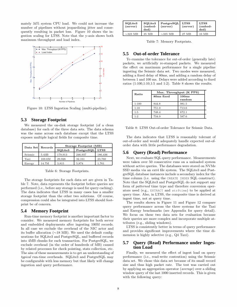
mately 34% system CPU load. We could not increase thenumber of pipelines without jeopardizing jitter and conse-quently resulting in packet loss. Figure 10 shows the in-gestion scaling for LTSS. Note that the y-axis shows bothmaximum throughput and load index.

Figure 10: LTSS Ingestion Scaling (multi-pipeline).

5.3 Storage FootprintWe measured the on-disk storage footprint (of a clean

database) for each of the three data sets. The data schemawas the same across each database except that the LTSSexposes multiple logical fields for composite time.

Data Set RecordsStorage Footprint (MB)

SQLite3 PostgreSQL LTSS

Seismic 5.43B 179,913 246,937 186,436

Taxi 169.6M 29,926 32,161 23,760

Energy 14.7M 3,815 5,874 1,761

Table 6: Storage Footprints.

The storage footprints for each data set are given in Ta-ble 7. Note, data represents the footprint before queries areperformed (i.e., before any storage is used for query caching).The data indicates that LTSS in many cases has a smallerstorage footprint than the other two solutions. Of course,compression could also be integrated into LTSS should foot-print be of concern.

5.4 Memory FootprintRun-time memory footprint is another important factor to

consider. We measured memory footprints for both serverand embedded deployments after ingesting 100M records.In all case we exclude the overhead of the NIC actor andits buffer allocation (∼18 MB). We used the default config-urations for SQLite3 and PostgreSQL, and buffered recordsinto 4MB chunks for each transaction. For PostgreSQL, weexclude overhead (in the order of hundreds of MB) causedby related processes for check pointing, stats collection, etc.The aim of these measurements is to get an understanding oftypical run-time overheads. SQLite3 and PostgreSQL maybe configurable with less memory but that likely will changeingestion and query performance.

SQLite3(server)

SQLite3(embed-ded)

PostgreSQL(server)

LTSS(server)

LTSS(embed-ded)

∼323 MB 35 MB ∼335 MB 27 MB 16 MB

Table 7: Memory Footprints.

5.5 Out-of-order ToleranceTo examine the tolerance for out-of-order (generally late)

packets, we artificially re-stamped packets. We measuredthe effect on maximum performance for a single pipelineingesting the Seismic data set. Two modes were measured,adding a fixed delay of 80ms, and adding a random delay ofbetween 1 and 100 ms. Delays were added according to fixedratios (1:100,1:10,1:5 and 1:2). Table 8 shows the results.

RatioMax. Throughput (K PPS)

80ms fixed 100msrandom

1:100 844.8 981.5

1:10 751.0 713.6

1:5 748.4 672.1

1:2 734.9 587.6

Table 8: LTSS Out-of-order Tolerance for Seismic Data.

The data indicates that LTSS is reasonably tolerant ofout-of-order and would adequately handle expected out-of-order data with little performance degradation.

5.6 Query (Read) PerformanceNext, we evaluate SQL query performance. Measurements

were taken over 50 consecutive runs on a unloaded systemwithout active queries. The databases were stored on NVMeSSD media via an ext4 file system. The SQLite3 and Post-greSQL database instances include a secondary index for thetime column (i.e. using the CREATE INDEX SQL construct).Note that the SQLite3 and PostgreSQL do not support anyform of patterned time type and therefore conversion oper-ators need (e.g., EXTRACT and strftime) to be applied atquery time. Also, in LTSS, the composite time is derived atingest time, not at query time.

The results shown in Figure 11 and Figure 12 comparequery performance across the three systems for the Taxiand Energy benchmarks (see Appendix for query detail).We focus on these two data sets for evaluation becausetheir queries are more complex and incorporate multiple at-tributes (e.g., sliding windows).

LTSS is consistently better in terms of query performanceand provides significant improvements where the time di-mension is highly selective (e.g., Q4 Taxi).

5.7 Query (Read) Performance under Inges-tion Load

Finally, we measured the effect of ingest load on queryperformance (i.e., read-write contention) using the Seismicdata set. We chose this data set because of its small recordsize and thus high packet rate. The test was carried outby applying an aggregation operator (average) over a slidingwindow query of the last 1000 inserted records. This is givenwith the following query:

8

Q1 Q2 Q3 Q4 Q5 Q6 Q7Query

0

50

100

150

200

250

300Ex

ecution Time (sec

onds

)SQLite3PostgresLTSS

Figure 11: NYC Taxi Query Performance.

Q1 Q2 Q3 Q4 Q5 Q6 Q7Query

0

10

20

30

40

50

60

70

80

Exec

ution Time (sec

onds

)

SQLite3PostgresLTSS

Figure 12: Belkin Energy Query Performance.

WITH vals(v) AS(SELECT value FROM seismic LIMIT 1000)

SELECT avg(v) FROM vals;

Query rate (QPS) was taken as a mean across 40 runs eachwith 20 windows. The data in Figure 13 shows fluctuationsin performance of less that 1% on increasing ingestion rateup to 1M events/sec in a single pipeline.

We do not include results for read-write contention onSQLite3 and PostgreSQL because they perform badly due totheir locking architectures. We were unable to avoid packetdrop under any reasonable query load (even with the clientopened in read-only mode).

6. CONCLUSIONSContinued evolution of IoT will bring with it a need to ag-

gregate, process and store large volumes of time-series data.In this paper we have presented a lightweight architecturefor storage and indexing of time-series data streams withinthe context of IoT. Our system, LTSS, is based on a soft-ware pipeline architecture that is optimized for multicoreprocessing and parallel IO capabilities. The architecture

Figure 13: Read-Write Contention for LTSS.

is specifically designed to take advantage of fast, random-access friendly, non-volatile storage devices (e.g., NVMe)and aims to reduce the dependency on DRAM by simplify-ing in-memory data structures. The result is a design thatcan be readily deployed on both commodity server as wellas resource constrained and embedded environments.

Our results show a data ingest (completely to persistentstore) in the order of 4 million RPS (without UDP packing)for a single 10G NIC with a load index of 14. For the Rasp-berry Pi 2 embedded platform, we show an ingest capabilityof around 70K RPS. These results are 3x to 4x improvementover existing RDBMS solutions. We also show that ad-hocquery performance, using SQL, is significantly better thanthat achievable with two prominent databases, SQLite3 andPostgres. Our solution currently does not employ compres-sion although there is no fundamental reason why this couldnot be added should a need arise.

We believe that this work represents a first step to consid-ering the increasing shift from IO-bound to CPU-bound dataprocessing and management. Careful consideration of dataflow across multiple processor cores and optimized mem-ory management is now becoming a fundamental element ofsuccessful high-performance stream processing and storagedesigns.

7. REFERENCES[1] Exokernel development kit (xdk).

https://github.com/dwaddington/xdk.Accessed: 2016-01-06.

[2] Ibm informix timeseries data user’s guide. Accessed:2016-01-21.

[3] Infiniflux: The world’s fastest time series dbms for iotand big data. http://www.infiniflux.com/.Accessed: 2016-01-21.

[4] Parstream db:The engine inside parstreams analytics platform for iot.https://www.parstream.com/product/parstream-db/.Accessed: 2016-01-14.

[5] Pipeline db documentation.http://docs.pipelinedb.com/. Accessed:2016-01-21.

[6] Protocol buffers.https://developers.google.com/protocol-buffers/.Accessed: 2016-01-04.

[7] Sap businessobject business intelligence.http://go.sap.com/product/analytics/bi-platform.htmlAccessed: 2016-01-26.

[8] Sas analytics platform.http://support.sas.com/documentation/onlinedoc/apcore/Accessed: 2016-01-26.

9

[9] Tableau business intelligence.http://www.tableau.com/business-intelligence.Accessed: 2016-01-26.

[10] Technical whitepaper: Real-time database for big dataanalytics. http://static1.squarespace.com/.Accessed: 2016-01-14.

[11] The virtual table mechanism of sqlite.https://www.sqlite.org/vtab.html. Accessed:2015-12-10.

[12] C. R. Cook and D. J. Kim. Best sorting algorithm fornearly sorted lists. Commun. ACM, 23(11):620–624,Nov. 1980.

[13] T. H. Cormen, C. Stein, R. L. Rivest, and C. E.Leiserson. Introduction to Algorithms. McGraw-HillHigher Education, 2nd edition, 2001.

[14] R. A. Elmasri and S. B. Navathe. Fundamentals of

Database Systems. Addison-Wesley LongmanPublishing Co., Inc., Boston, MA, USA, 3rd edition,1999.

[15] J. Groff and P. Weinberg. SQL The Complete

Reference, 3rd Edition. McGraw-Hill, Inc., New York,NY, USA, 3 edition, 2010.

[16] N. H. Jorg Bienert, Michael Hummel. Method andsystem for compressing data records and forprocessing, August 2013.

[17] J. Kuang, D. G. Waddington, and C. Lin. Techniquesfor fast and scalable time series traffic generation. InProceedings of the 2015 IEEE Conference on Big

Data, BigData’15, Oct. 2015.

[18] P. O’Neil, E. Cheng, D. Gawlick, and E. O’Neil. Thelog-structured merge-tree (lsm-tree), 1996.

[19] D. Rogerson. COM. Microsoft programming series.Microsoft Press, 1997.

[20] M. Zaharia, M. Chowdhury, M. J. Franklin,S. Shenker, and I. Stoica. Spark: Cluster computingwith working sets. In Proceedings of the 2Nd USENIX

Conference on Hot Topics in Cloud Computing,HotCloud’10, pages 10–10, Berkeley, CA, USA, 2010.USENIX Association.

10

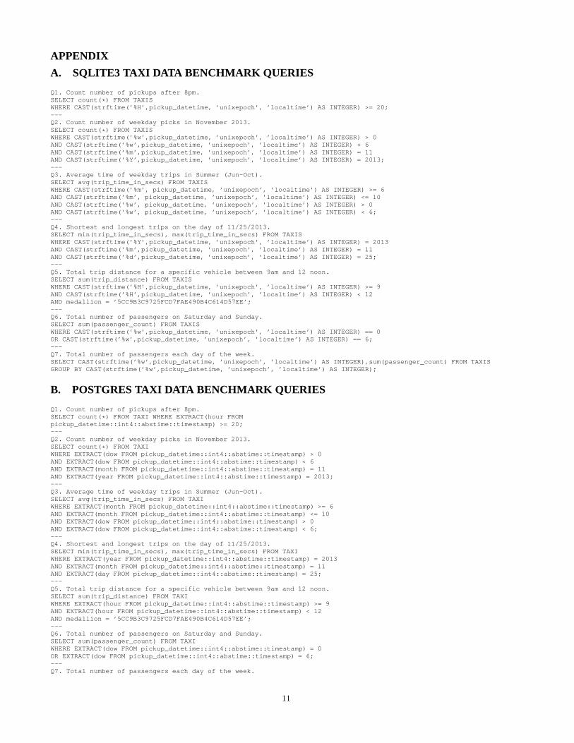
APPENDIX

A. SQLITE3 TAXI DATA BENCHMARK QUERIES

Q1. Count number of pickups after 8pm.SELECT count(*) FROM TAXISWHERE CAST(strftime(’%H’,pickup_datetime, ’unixepoch’, ’localtime’) AS INTEGER) >= 20;---Q2. Count number of weekday picks in November 2013.SELECT count(*) FROM TAXISWHERE CAST(strftime(’%w’,pickup_datetime, ’unixepoch’, ’localtime’) AS INTEGER) > 0AND CAST(strftime(’%w’,pickup_datetime, ’unixepoch’, ’localtime’) AS INTEGER) < 6AND CAST(strftime(’%m’,pickup_datetime, ’unixepoch’, ’localtime’) AS INTEGER) = 11AND CAST(strftime(’%Y’,pickup_datetime, ’unixepoch’, ’localtime’) AS INTEGER) = 2013;---Q3. Average time of weekday trips in Summer (Jun-Oct).SELECT avg(trip_time_in_secs) FROM TAXISWHERE CAST(strftime(’%m’, pickup_datetime, ’unixepoch’, ’localtime’) AS INTEGER) >= 6AND CAST(strftime(’%m’, pickup_datetime, ’unixepoch’, ’localtime’) AS INTEGER) <= 10AND CAST(strftime(’%w’, pickup_datetime, ’unixepoch’, ’localtime’) AS INTEGER) > 0AND CAST(strftime(’%w’, pickup_datetime, ’unixepoch’, ’localtime’) AS INTEGER) < 6;---Q4. Shortest and longest trips on the day of 11/25/2013.SELECT min(trip_time_in_secs), max(trip_time_in_secs) FROM TAXISWHERE CAST(strftime(’%Y’,pickup_datetime, ’unixepoch’, ’localtime’) AS INTEGER) = 2013AND CAST(strftime(’%m’,pickup_datetime, ’unixepoch’, ’localtime’) AS INTEGER) = 11AND CAST(strftime(’%d’,pickup_datetime, ’unixepoch’, ’localtime’) AS INTEGER) = 25;---Q5. Total trip distance for a specific vehicle between 9am and 12 noon.SELECT sum(trip_distance) FROM TAXISWHERE CAST(strftime(’%H’,pickup_datetime, ’unixepoch’, ’localtime’) AS INTEGER) >= 9AND CAST(strftime(’%H’,pickup_datetime, ’unixepoch’, ’localtime’) AS INTEGER) < 12AND medallion = ’5CC9B3C9725FCD7FAE490B4C614D57EE’;---Q6. Total number of passengers on Saturday and Sunday.SELECT sum(passenger_count) FROM TAXISWHERE CAST(strftime(’%w’,pickup_datetime, ’unixepoch’, ’localtime’) AS INTEGER) == 0OR CAST(strftime(’%w’,pickup_datetime, ’unixepoch’, ’localtime’) AS INTEGER) == 6;---Q7. Total number of passengers each day of the week.SELECT CAST(strftime(’%w’,pickup_datetime, ’unixepoch’, ’localtime’) AS INTEGER),sum(passenger_count) FROM TAXISGROUP BY CAST(strftime(’%w’,pickup_datetime, ’unixepoch’, ’localtime’) AS INTEGER);

B. POSTGRES TAXI DATA BENCHMARK QUERIES

Q1. Count number of pickups after 8pm.SELECT count(*) FROM TAXI WHERE EXTRACT(hour FROMpickup_datetime::int4::abstime::timestamp) >= 20;---Q2. Count number of weekday picks in November 2013.SELECT count(*) FROM TAXIWHERE EXTRACT(dow FROM pickup_datetime::int4::abstime::timestamp) > 0AND EXTRACT(dow FROM pickup_datetime::int4::abstime::timestamp) < 6AND EXTRACT(month FROM pickup_datetime::int4::abstime::timestamp) = 11AND EXTRACT(year FROM pickup_datetime::int4::abstime::timestamp) = 2013;---Q3. Average time of weekday trips in Summer (Jun-Oct).SELECT avg(trip_time_in_secs) FROM TAXIWHERE EXTRACT(month FROM pickup_datetime::int4::abstime::timestamp) >= 6AND EXTRACT(month FROM pickup_datetime::int4::abstime::timestamp) <= 10AND EXTRACT(dow FROM pickup_datetime::int4::abstime::timestamp) > 0AND EXTRACT(dow FROM pickup_datetime::int4::abstime::timestamp) < 6;---Q4. Shortest and longest trips on the day of 11/25/2013.SELECT min(trip_time_in_secs), max(trip_time_in_secs) FROM TAXIWHERE EXTRACT(year FROM pickup_datetime::int4::abstime::timestamp) = 2013AND EXTRACT(month FROM pickup_datetime::int4::abstime::timestamp) = 11AND EXTRACT(day FROM pickup_datetime::int4::abstime::timestamp) = 25;---Q5. Total trip distance for a specific vehicle between 9am and 12 noon.SELECT sum(trip_distance) FROM TAXIWHERE EXTRACT(hour FROM pickup_datetime::int4::abstime::timestamp) >= 9AND EXTRACT(hour FROM pickup_datetime::int4::abstime::timestamp) < 12AND medallion = ’5CC9B3C9725FCD7FAE490B4C614D57EE’;---Q6. Total number of passengers on Saturday and Sunday.SELECT sum(passenger_count) FROM TAXIWHERE EXTRACT(dow FROM pickup_datetime::int4::abstime::timestamp) = 0OR EXTRACT(dow FROM pickup_datetime::int4::abstime::timestamp) = 6;---Q7. Total number of passengers each day of the week.

11

SELECT EXTRACT(dow FROM pickup_datetime::int4::abstime::timestamp),sum(passenger_count) FROM TAXIGROUP BY EXTRACT(dow FROM pickup_datetime::int4::abstime::timestamp);

C. LTSS TAXI DATA BENCHMARK QUERIES

Q1. Count number of pickups after 8pm.SELECT count(*) FROM TAXI WHERE CTIME_pickup_hour >= 20;---Q2. Count number of weekday picks in November 2013.SELECT count(*) FROM TAXI WHERE CTIME_pickup_wday > 0AND CTIME_pickup_wday < 6AND CTIME_pickup_month = 11 AND CTIME_pickup_year = 13;---Q3. Average time of weekday trips in Summer (Jun-Oct).SELECT avg(trip_time_in_secs) FROM TAXIWHERE CTIME_pickup_month >= 6 AND CTIME_pickup_month <= 10AND CTIME_pickup_wday > 0 AND CTIME_pickup_wday < 6;---Q4. Shortest and longest trips on the day of 11/25/2013.SELECT min(trip_time_in_secs), max(trip_time_in_secs) FROM TAXIWHERE CTIME_pickup_year = 13 AND CTIME_pickup_month = 11AND CTIME_pickup_day = 25;---Q5. Total trip distance for a specific vehicle between 9am and 12 noon.SELECT sum(trip_distance) FROM TAXI WHERE CTIME_pickup_hour >= 9AND CTIME_pickup_hour < 12AND medallion = ’5CC9B3C9725FCD7FAE490B4C614D57EE’;---Q6. Total number of passengers on Saturday and Sunday.SELECT sum(passenger_count) FROM TAXI WHERE CTIME_pickup_wday == 0OR CTIME_pickup_wday == 6;---Q7. Total number of passengers each day of the week.SELECT CTIME_pickup_wday,sum(passenger_count) FROM TAXIGROUP BY CTIME_pickup_wday;

D. SQLITE3 ENERGY DATA BENCHMARK QUERIES

Q1. Hourly average power consumption for house H1.SELECT strftime(’%H’,DATETIME), avg(V0 * I0) FROM POWERWHERE HOUSEID = ’H1’ GROUP BY strftime(’%H’,DATETIME);---Q2. Maximum power sample for each house.SELECT HOUSEID, max(V0*I0) FROM POWERWHERE CAST(strftime(’%H’,DATETIME) AS INTEGER) > 8 AND CAST(strftime(’%H’,DATETIME) AS INTEGER) <= 20GROUP BY HOUSEID ORDER BY HOUSEID;---Q3. Highest hourly average power sample point for each house.WITH

hourlies (HOUSEID, HOUR, POWER) AS (SELECT HOUSEID, strftime(’%H’,DATETIME), avg(V0 * I0) FROM POWERGROUP BY HOUSEID, strftime(’%H’,DATETIME) ORDER BY avg(V0*I0) DESC)SELECT HOUSEID, HOUR, max(POWER) FROM hourliesWHERE HOUSEID IN (SELECT DISTINCT HOUSEID FROM POWER)---Q4. Top ten, 5 minute periods of consumption from house ’H1’ (tumbling window).SELECT HOUSEID, avg(V0*I0), (strftime(’%s’,DATETIME)/300) FROM POWERWHERE HOUSEID=’H1’ GROUP BY HOUSEID, (strftime(’%s’,DATETIME)/300) ORDER BY (strftime(’%s’,DATETIME)/300) DESC LIMIT 10;---Q5. Number of samples between two datetimesSELECT count(*) FROM POWER WHERE DATETIME >= ’2012-07-30 09:35:00’ AND DATETIME <= ’2012-07-30 09:39:00’;---Q6. Average maxium weekday consumption for each house.WITH

weekday_max(houseid, wdaymax, power)AS (

SELECT HOUSEID, strftime(’%w’,DATETIME), max(V0*I0)FROM POWERGROUP BY HOUSEID, (strftime(’%w’,DATETIME))

)SELECT houseid, avg(power) FROM weekday_max GROUP BY houseid ORDER BY houseid;---Q7. Number of samples taken between 5pm and 9pm on Wednesday.SELECT count(*) FROM POWER WHERE strftime(’%w’,DATETIME) = ’3’AND CAST(strftime(’%H’,DATETIME) as INTEGER) >= 17 AND CAST(strftime(’%H’,DATETIME) as INTEGER) <= 20;

E. POSTGRES ENERGY DATA BENCHMARK QUERIES

12

Q1. Hourly average power consumption for house H1.SELECT EXTRACT(hour FROM DATETIME), avg(V0 * I0) FROM POWERWHERE HOUSEID = ’H1’ GROUP BY EXTRACT(hour FROM DATETIME);---Q2. Maximum power sample for each house.SELECT HOUSEID, max(V0*I0) FROM POWERWHERE EXTRACT(hour FROM DATETIME) > 8 AND EXTRACT(hour FROM DATETIME) <= 20GROUP BY HOUSEID ORDER BY HOUSEID;---Q3. Highest hourly average power sample point for each house.WITH hourlies (HOUSEID, HOUR, POWER) AS (

SELECT HOUSEID, EXTRACT(hour FROM DATETIME), avg(V0 * I0)FROM POWERGROUP BY HOUSEID, EXTRACT(hour FROM DATETIME)ORDER BY avg(V0*I0) DESC)

SELECT * FROM ( SELECT DISTINCT ON (HOUSEID) * FROM hourlies ORDER BY HOUSEID ) qORDER BY q.houseid;---Q4. Top ten, 5 minute periods of consumption from house ’H1’ (tumbling window).WITH fives(houseid, avgpower) AS (

SELECT HOUSEID, avg(V0*10) FROM POWERWHERE HOUSEID=’H1’GROUP BY HOUSEID, (cast(EXTRACT(EPOCH FROM DATETIME) as int)/300)ORDER BY HOUSEID )

SELECT fives.houseid, avgpower FROM fives ORDER BY fives.avgpower DESC LIMIT 10;---Q5. Number of samples between two datetimesSELECT count(*) FROM POWER WHERE DATETIME >= ’2012-07-30 09:35:00’AND DATETIME <= ’2012-07-30 09:39:00’;---Q6. Average maxium weekday consumption for each house.WITH weekday_max(houseid, wdaymax, power) AS (

SELECT HOUSEID, EXTRACT(dow FROM DATETIME), max(V0*I0)FROM POWER GROUP BY HOUSEID, EXTRACT(dow FROM DATETIME)

)SELECT houseid, avg(power) FROM weekday_max GROUP BY houseid ORDER BY houseid;---Q7. Number of samples taken between 5pm and 9pm on Wednesday.SELECT count(*) FROM POWERWHERE EXTRACT(dow FROM DATETIME) = 3 AND EXTRACT(hour FROM DATETIME) >= 17AND EXTRACT(hour FROM DATETIME) <= 20;

F. LTSS ENERGY DATA BENCHMARK QUERIES

Q1. Hourly average power consumption for house H1.SELECT CTIME_hour, avg(V0*I0) FROM POWER WHERE HOUSEID = ’H1’GROUP BY CTIME_hour ORDER BY CTIME_hour;---Q2. Maximum power sample for each house.SELECT HOUSEID, max(V0*I0) FROM POWERWHERE CTIME_hour > 8 AND CTIME_hour < 20 GROUP BY HOUSEID ORDER BY HOUSEID;---Q3. Highest hourly average power sample point for each house.WITH hourlies (HOUSEID, HOUR, POWER) AS (SELECT HOUSEID, CTIME_hour, avg(V0*I0)

FROM POWER GROUP BY HOUSEID, CTime_hour ORDER BY avg(V0*I0) DESC)SELECT HOUSEID, HOUR, max(POWER) FROM hourliesWHERE HOUSEID IN (SELECT DISTINCT HOUSEID FROM POWER) GROUP BY HOUSEID;---Q4. Top ten, 5 minute periods of consumption from house ’H1’ (tumbling window).SELECT HOUSEID, avg(V0*I0), (TIMESTAMP / 300000000) FROM POWERWHERE HOUSEID=’H1’ GROUP BY HOUSEID, (TIMESTAMP / 300000000)ORDER BY (TIMESTAMP / 300000000) DESC LIMIT 10;---Q5. Number of samples between two datetimesSELECT count(*) FROM POWER WHERE CTIME_year = 12 AND CTIME_month = 7AND CTIME_day = 30 AND CTIME_hour = 9 AND CTIME_min >= 35 AND CTIME_min < 39;---Q6. Average maxium weekday consumption for each house.WITH weekday_max(houseid, wdaymax, power) AS (

SELECT HOUSEID, CTIME_wday, max(V0*I0)FROM POWER GROUP BY HOUSEID, CTIME_wday)

SELECT houseid, avg(power) FROM weekday_maxGROUP BY houseid ORDER BY houseid;---Q7. Number of samples taken between 5pm and 9pm on Wednesday.SELECT count(*) FROM POWER WHERE CTIME_wday = 3 AND CTIME_hour >= 17AND CTIME_hour <= 20;

13