a fast simulation method for 1d heat conduction · a fast simulation method for 1d heat conduction...

This document contains a post-print version of the paper

A fast simulation method for 1D heat conduction

authored by A. Steinboeck, D. Wild, T. Kiefer, and A. Kugi

and published in Mathematics and Computers in Simulation.

The content of this post-print version is identical to the published paper but without the publisher’s final layout orcopy editing. Please, scroll down for the article.

Cite this article as:A. Steinboeck, D. Wild, T. Kiefer, and A. Kugi, “A fast simulation method for 1D heat conduction”, Mathematics andComputers in Simulation, vol. 82, no. 3, pp. 392–403, 2011. doi: 10.1016/j.matcom.2010.10.016

BibTex entry:@ARTICLE{steinboeck11a,AUTHOR = {Steinboeck, A. and Wild, D. and Kiefer, T. and Kugi, A.},TITLE = {A fast simulation method for 1{D} heat conduction},JOURNAL = {Mathematics and Computers in Simulation},YEAR = {2011},volume = {82},number = {3},pages = {392-403},doi = {10.1016/j.matcom.2010.10.016},url = {http://www.sciencedirect.com/science/article/pii/S037847541000323X}

}

Link to original paper:http://dx.doi.org/10.1016/j.matcom.2010.10.016http://www.sciencedirect.com/science/article/pii/S037847541000323X

Read more ACIN papers or get this document:http://www.acin.tuwien.ac.at/literature

Contact:Automation and Control Institute (ACIN) Internet: www.acin.tuwien.ac.atVienna University of Technology E-mail: [email protected] 27-29/E376 Phone: +43 1 58801 376011040 Vienna, Austria Fax: +43 1 58801 37699

Copyright notice:This is the authors’ version of a work that was accepted for publication in Mathematics and Computers in Simulation. Changes resultingfrom the publishing process, such as peer review, editing, corrections, structural formatting, and other quality control mechanisms may notbe reflected in this document. Changes may have been made to this work since it was submitted for publication. A definitive version wassubsequently published in A. Steinboeck, D. Wild, T. Kiefer, and A. Kugi, “A fast simulation method for 1D heat conduction”, Mathematicsand Computers in Simulation, vol. 82, no. 3, pp. 392–403, 2011. doi: 10.1016/j.matcom.2010.10.016

http://dx.doi.org/10.1016/j.matcom.2010.10.016


http://www.sciencedirect.com/science/article/pii/S037847541000323X

http://www.acin.tuwien.ac.at/literature

www.acin.tuwien.ac.at

mailto:[email protected]


A fast simulation method for 1D heat conduction✩

A. Steinboeck∗,a, D. Wildb, T. Kieferb, A. Kugia

aAutomation and Control Institute, Vienna University of Technology, Gusshausstrasse 27–29, 1040 Wien, AustriabAG der Dillinger Huttenwerke, Werkstrasse 1, 66763 Dillingen/Saar, Germany

Abstract

A flexible solution method for the initial-boundary value problem of the temperature field in a one-dimensional do-main of a solid with significantly nonlinear material parameters and radiation boundary conditions is proposed. Atransformation of the temperature values allows to isolatethe nonlinear material characteristics into a single coeffi-cient of the heat conduction equation. The Galerkin method is utilized for spatial discretization of the problem andintegration of the time domain is done by constraining the boundary heat fluxes to piecewise linear, discontinuoussignals. The radiative heat exchange is computed with the help of the Stefan-Boltzmann law, such that the ambienttemperatures serve as system inputs. The feasibility and accuracy of the proposed method are demonstrated by meansof an example of heat treatment of a steel slab, where numerical results are compared to the finite difference method.

Key words: heat conduction, nonlinear material parameters, method ofweighted residuals, Galerkin method,radiative heat exchange, implicit difference equation

1. Introduction

In process control applications, there is a need for mathematical models which are both computationally inex-pensive as well as reliable in terms of accuracy and convergence. These requirements are particularly important formodels to be used in real-time applications like trajectoryplanning, optimization, or control. Motivated by theseneeds, a method to determine the transient temperature fieldin a one-dimensional domain of a solid with significantlynonlinear material parameters and radiation boundary conditions is proposed. The approach originates from an ap-plication in the steel industry, where slabs or rolled products are to be heat-treated or reheated according to specifictemperature trajectories [2, 21, 22]. However, by analogy,the method can be applied to other diffusion-convectionsystems described by parabolic initial-boundary value problems.

The paper is organized as follows: Section 2 starts with a brief review of the heat conduction equation (strongformulation) with nonlinear material parameters and Neumann boundary conditions, followed by a transformation ofthe temperature such that the nonlinearity is isolated intoa single parameter of the parabolic problem. Thereupon, theproblem is restated in the weak formulation, which is suitable for the Method of Weighted Residuals (MWR). Here,the Galerkin Method (GM) is employed to derive a low-dimensional lumped-parameter system, and a time integrationmethod is proposed which allows for piecewise linear, discontinuous input signals. Finally, the boundary conditionsare supplemented by elementary laws of thermal radiation. The feasibility and the accuracy of the proposed methodare examined by means of an example of heat treatment of a steel slab in Section 3. For comparison, also the FiniteDifference Method (FDM) is applied to the problem under consideration. A brief overview of the assumptions andapproximations utilized in this work is given in the final Section 4.

✩A preliminary version of this paper was presented at the 6th Vienna Conference on Mathematical Modelling in February 2009, cf. [20].∗Corresponding author.Email address:[email protected] (A. Steinboeck)

Preprint submitted to Mathematics and Computers in Simulation October 22, 2010

Post-print version of the article: A. Steinboeck, D. Wild, T. Kiefer, and A. Kugi, “A fast simulation method for 1D heat conduction”,Mathematics and Computers in Simulation, vol. 82, no. 3, pp. 392–403, 2011. doi: 10.1016/j.matcom.2010.10.016The content of this post-print version is identical to the published paper but without the publisher’s final layout or copy editing.


2. Theoretical concept

2.1. Heat conduction problem with Neumann boundary conditions

yL/2

−L/2

q+(t)

q−(t)

T(y, t)

T+w(t)

T−w(t)

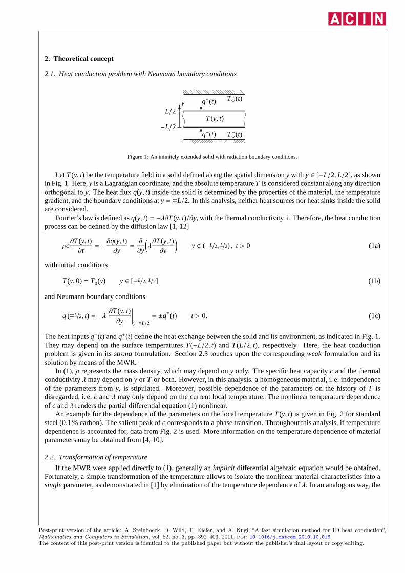
Figure 1: An infinitely extended solid with radiation boundary conditions.

Let T(y, t) be the temperature field in a solid defined along the spatial dimensiony with y ∈ [−L/2, L/2], as shownin Fig. 1. Here,y is a Lagrangian coordinate, and the absolute temperatureT is considered constant along any directionorthogonal toy. The heat fluxq(y, t) inside the solid is determined by the properties of the material, the temperaturegradient, and the boundary conditions aty = ∓L/2. In this analysis, neither heat sources nor heat sinks inside the solidare considered.

Fourier’s law is defined asq(y, t) = −λ∂T(y, t)/∂y, with the thermal conductivityλ. Therefore, the heat conductionprocess can be defined by the diffusion law [1, 12]

ρc∂T(y, t)∂t

= −∂q(y, t)∂y

=∂

∂y

(

λ∂T(y, t)∂y

)

y ∈ (−L/2, L/2) , t > 0 (1a)

with initial conditions

T(y, 0) = T0(y) y ∈ [−L/2, L/2] (1b)

and Neumann boundary conditions

q (∓L/2, t) = −λ∂T(y, t)∂y

∣∣∣∣∣y=∓L/2

= ±q∓(t) t > 0. (1c)

The heat inputsq−(t) andq+(t) define the heat exchange between the solid and its environment, as indicated in Fig. 1.They may depend on the surface temperaturesT(−L/2, t) and T(L/2, t), respectively. Here, the heat conductionproblem is given in itsstrong formulation. Section 2.3 touches upon the correspondingweak formulation and itssolution by means of the MWR.

In (1), ρ represents the mass density, which may depend ony only. The specific heat capacityc and the thermalconductivityλ may depend ony or T or both. However, in this analysis, a homogeneous material,i. e. independenceof the parameters fromy, is stipulated. Moreover, possible dependence of the parameters on the history ofT isdisregarded, i. e.c andλ may only depend on the current local temperature. The nonlinear temperature dependenceof c andλ renders the partial differential equation (1) nonlinear.

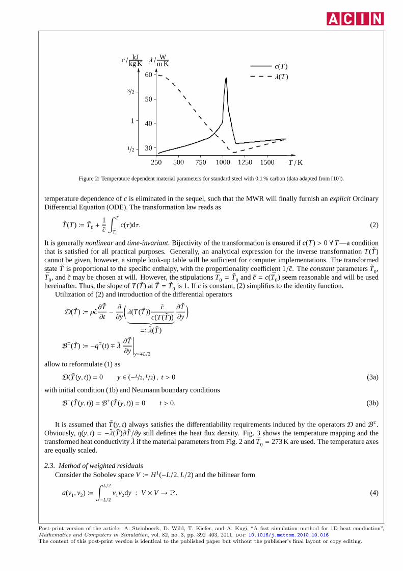
An example for the dependence of the parameters on the local temperatureT(y, t) is given in Fig. 2 for standardsteel (0.1 % carbon). The salient peak ofc corresponds to a phase transition. Throughout this analysis, if temperaturedependence is accounted for, data from Fig. 2 is used. More information on the temperature dependence of materialparameters may be obtained from [4, 10].

2.2. Transformation of temperature

If the MWR were applied directly to (1), generally animplicit differential algebraic equation would be obtained.Fortunately, a simple transformation of the temperature allows to isolate the nonlinear material characteristics into asingleparameter, as demonstrated in [1] by elimination of the temperature dependence ofλ. In an analogous way, the



1/2

1

3/2

250 500 750 1000 1250 1500

30

40

50

60 λ(T)

c(T)c / kJ

kg K λ / Wm K

T /K

Figure 2: Temperature dependent material parameters for standard steel with 0.1 % carbon (data adapted from [10]).

temperature dependence ofc is eliminated in the sequel, such that the MWR will finally furnish anexplicit OrdinaryDifferential Equation (ODE). The transformation law reads as

T(T) ≔ T0 +1c

∫ T

T0

c(τ)dτ. (2)

It is generallynonlinearandtime-invariant. Bijectivity of the transformation is ensured ifc(T) > 0 ∀T—a conditionthat is satisfied for all practical purposes. Generally, an analytical expression for the inverse transformationT(T)cannot be given, however, a simple look-up table will be sufficient for computer implementations. The transformedstateT is proportional to the specific enthalpy, with the proportionality coefficient 1/c. TheconstantparametersT0,T0, andc may be chosen at will. However, the stipulationsT0 = T0 andc = c(T0) seem reasonable and will be usedhereinafter. Thus, the slope ofT(T) at T = T0 is 1. If c is constant, (2) simplifies to the identity function.

Utilization of (2) and introduction of the differential operators

D(T) ≔ ρc∂T∂t−∂

∂y

(

λ(T(T))c

c(T(T))︸︷︷︸

≕ λ(T)

∂T∂y

)

B∓(T) ≔ −q∓(t) ∓ λ∂T∂y

∣∣∣∣∣∣y=∓L/2

allow to reformulate (1) as

D(T(y, t)) = 0 y ∈ (−L/2, L/2) , t > 0 (3a)

with initial condition (1b) and Neumann boundary conditions

B−(T(y, t)) = B+(T(y, t)) = 0 t > 0. (3b)

It is assumed thatT(y, t) always satisfies the differentiability requirements induced by the operatorsD andB∓.Obviously,q(y, t) = −λ(T)∂T/∂y still defines the heat flux density. Fig. 3 shows the temperature mapping and thetransformed heat conductivityλ if the material parameters from Fig. 2 andT0 = 273 K are used. The temperature axesare equally scaled.

2.3. Method of weighted residualsConsider the Sobolev spaceV ≔ H1(−L/2, L/2) and the bilinear form

a(v1, v2) ≔∫ L/2

−L/2v1v2dy : V × V → R. (4)



0

500

1000

1500

500 1000 1500 2000

20

40

60λ(T)

T(T)T /K λ / W

m K

T /K

Figure 3: Transformation of temperature and transformed heat conductivity for standard steel (0.1 % carbon).

Usinganytest functionv(y) ∈ V andanyscalar factorsv−, v+ ∈ R, the identity

a(v(y),D(T(y, t))) + v−B−(T(y, t)) + v+B+(T(y, t)) = 0

must hold for anyt > 0. Here,D(T(y, t)) ∈ L2(−L/2, L/2) and‖B∓(T(y, t))‖ < ∞ are required, whereL2(−L/2, L/2) isthe space of square integrable functions on the interval (−L/2, L/2). The usual way for obtaining the weak formulationis integration by parts (cf. [7, 16]), which yields

0 = a(

v(y), ρc∂T(y, t)∂t

)

+ a(∂v(y)∂y, λ(T(y, t))

∂T(y, t)∂y

)

− v−q−(t) − v+q+(t)

−(

v− − v(−L/2))

λ∂T(y, t)∂y

∣∣∣∣∣∣y=−L/2

+(

v+ − v(L/2))

λ∂T(y, t)∂y

∣∣∣∣∣∣y=L/2

t > 0.(5)

In this equation, the requirements on the differentiability of T(y, t) with respect toy are less restrictive than in theoperatorD. Apart from this fact, (3) and (5) are equivalent. Until now,there is no mathematical approximation,implying that the solution of (5) is identical to the solution of the strong formulations (1) and (3).

The basic idea of the MWR is to derive anapproximatesolution of (5) by restrictingT(y, t) to somefinite-dimensionalspace and by discarding the stipulation that (5) must be satisfied for anyv(y) ∈ V and anyv−, v+ ∈ R. Amathematically simple solution may be found if (5) only holds for anyv(y) ∈ Vh ⊆ V and anyv∓ ∈ V∓h ⊆ R, whereVhis afinite-dimensionalsubspace.

Clearly, the choicev∓ = v(∓L/2) causes the second line of (5) to vanish. This reasonable simplification isparticularly useful for Neumann boundary conditions [24].Hence, it is used throughout this paper. Unfortunately, thesecond term on the right-hand side of (5) contains the generally nonlinear functionλ(T(y, t)). Assuming for the timebeing thata(∂v(y)/∂y, ∂T(y, t)/∂y) , 0, the weighted mean value

λ = λ(v(y), T(y, t)) =a(∂v(y)∂y , λ(T(y, t)) ∂T(y,t)

∂y

)

a(∂v(y)∂y ,

∂T(y,t)∂y

) (6)

can be used to rewrite (5) as

0 = a(

v(y), ρc∂T(y, t)∂t

)

+ λ(v(y), T(y, t))a(∂v(y)∂y,∂T(y, t)∂y

)

− v (−L/2) q−(t) − v (L/2) q+(t) t > 0. (7)

Note that the parameterλ does not depend ony. In principle, the introduction of (6) does not entail any approximationerror. However, later some accuracy will be sacrificed to simplify time integration. For a computer implementation ofthe method, special care should be taken to avoid numerical problems if the denominator of (6) is close to zero. Forinstance,v(y) = const. or T(y, t) = const. w.r.t. y should automatically result inλ = 0.



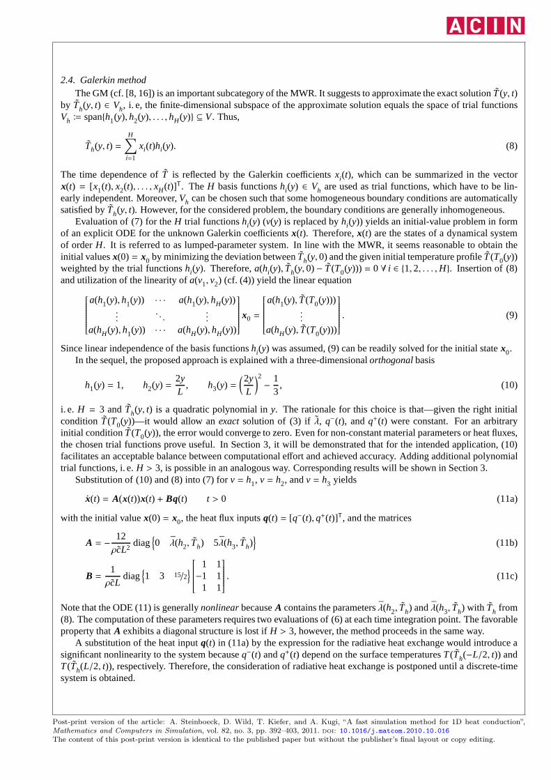
2.4. Galerkin methodThe GM (cf. [8, 16]) is an important subcategory of the MWR. Itsuggests to approximate the exact solutionT(y, t)

by Th(y, t) ∈ Vh, i. e, the finite-dimensional subspace of the approximate solution equals the space of trial functionsVh ≔ span{h1(y), h2(y), . . . , hH(y)} ⊆ V. Thus,

Th(y, t) =H∑

i=1

xi(t)hi(y). (8)

The time dependence ofT is reflected by the Galerkin coefficientsxi(t), which can be summarized in the vectorx(t) = [x1(t), x2(t), . . . , xH(t)]T. TheH basis functionshi(y) ∈ Vh are used as trial functions, which have to be lin-early independent. Moreover,Vh can be chosen such that some homogeneous boundary conditions are automaticallysatisfied byTh(y, t). However, for the considered problem, the boundary conditions are generally inhomogeneous.

Evaluation of (7) for theH trial functionshi(y) (v(y) is replaced byhi(y)) yields an initial-value problem in formof an explicit ODE for the unknown Galerkin coefficientsx(t). Therefore,x(t) are the states of a dynamical systemof orderH. It is referred to as lumped-parameter system. In line with the MWR, it seems reasonable to obtain theinitial valuesx(0) = x0 by minimizing the deviation betweenTh(y, 0) and the given initial temperature profileT(T0(y))weighted by the trial functionshi(y). Therefore,a(hi(y), Th(y, 0)− T(T0(y))) = 0 ∀ i ∈ {1, 2, . . . ,H}. Insertion of (8)and utilization of the linearity ofa(v1, v2) (cf. (4)) yield the linear equation

a(h1(y), h1(y)) · · · a(h1(y), hH(y))...

. . ....

a(hH(y), h1(y)) · · · a(hH(y), hH(y))

x0 =

a(h1(y), T(T0(y)))...

a(hH(y), T(T0(y)))

. (9)

Since linear independence of the basis functionshi(y) was assumed, (9) can be readily solved for the initial statex0.In the sequel, the proposed approach is explained with a three-dimensionalorthogonalbasis

h1(y) = 1, h2(y) =2yL

, h3(y) =(2y

L

)2

−13

, (10)

i. e. H = 3 andTh(y, t) is a quadratic polynomial iny. The rationale for this choice is that—given the right initialcondition T(T0(y))—it would allow anexactsolution of (3) if λ, q−(t), andq+(t) were constant. For an arbitraryinitial conditionT(T0(y)), the error would converge to zero. Even for non-constant material parameters or heat fluxes,the chosen trial functions prove useful. In Section 3, it will be demonstrated that for the intended application, (10)facilitates an acceptable balance between computational effort and achieved accuracy. Adding additional polynomialtrial functions, i. e.H > 3, is possible in an analogous way. Corresponding results will be shown in Section 3.

Substitution of (10) and (8) into (7) forv = h1, v = h2, andv = h3 yields

x(t) = A(x(t))x(t) + Bq(t) t > 0 (11a)

with the initial valuex(0) = x0, the heat flux inputsq(t) = [q−(t), q+(t)]T, and the matrices

A = −12ρcL2

diag{

0 λ(h2, Th) 5λ(h3, Th)}

(11b)

B =1ρcL

diag{

1 3 15/2}

1 1−1 1

1 1

. (11c)

Note that the ODE (11) is generallynonlinearbecauseA contains the parametersλ(h2, Th) andλ(h3, Th) with Th from(8). The computation of these parameters requires two evaluations of (6) at each time integration point. The favorableproperty thatA exhibits a diagonal structure is lost ifH > 3, however, the method proceeds in the same way.

A substitution of the heat inputq(t) in (11a) by the expression for the radiative heat exchange would introduce asignificant nonlinearity to the system becauseq−(t) andq+(t) depend on the surface temperaturesT(Th(−L/2, t)) andT(Th(L/2, t)), respectively. Therefore, the consideration of radiative heat exchange is postponed until a discrete-timesystem is obtained.



2.5. FOH-type time integration method

Any standard numerical ODE solver algorithm for explicit initial-value problems should suffice to integrate (11).However, the benefit of manual discretization of the system is that usually laborious iterative solver algorithms canbe replaced by algebraic difference equations, which allow rapid evaluation. Consider adiscretized time domain withsampling instantstk ∀ k ∈ N, which are generallynotequidistant, and letTk = tk+1− tk be the corresponding samplingperiod.

u(t)uk

tt tk−1tk−1 tktk tk+1tk+1TkTk

q1∓k

q2∓k

q∓(t)

a) b)

Figure 4: Shape of input signal, a) ZOH method, b) FOH-type method.

In order to obtain a discrete-time representation [9, 14] ofa state space system like (11), the Zero-Order-Hold(ZOH) method [9, 15] is frequently applied. ZOH means that any input is forced to a function space which has thestep functionsσ(t− tk) ∀ k ∈ N as a basis, as exemplified in Fig. 4.a for some scalar inputu(t). Inspired by the fact thatthe First-Order-Hold (FOH) method [9, 15] furnishes more accurate results than the ZOH method, a time integrationmethod capable ofpiecewise linearinput signals is outlined in the following. Moreover, the considered function spaceallows fordiscontinuousinput signals, which may occur in process control applications. Sampling pointstk must beset at least at discontinuities of the input signals or theirslope. Then, the inputq(t) of (11a) can be defined as

q(t) = q1k

tk+1 − t

Tk

+ q2k

t − tkTk

for tk ≤ t < tk+1 (12)

with q1k = [q1−

k , q1+k ]T and q2

k = [q2−k , q

2+k ]T. The meaning of these vectors is illustrated in Fig. 4.b. However, the

componentsq−(t) andq+(t) are generally not equal. The vectors may be obtained from

q1k = q(tk), q2

k = limτ→0−

q(tk+1 + τ).

The series (q1k) and (q2

k) are the inputs to the discretized system. In order to facilitate a simple analytical solution ofthe ODE (11), it is assumed that the parametersλ(h2, Th) and λ(h3, Th) take theconstantvaluesλ(h2, Th(y, tk)) andλ(h3, Th(y, tk)) within each time interval [tk, tk+1). Implementing thisapproximation, the integration of (11) with theinput (12) readily yields the discrete-time system

xk+1 = Ak(xk)xk + B1k(xk)q1

k + B2k(xk)q2

k (13a)

with

Ak = diag{

1 exp(−12λ(h2,Th(y,tk))Tk

ρcL2

)

exp(−60λ(h3,Th(y,tk))Tk

ρcL2

)}

(13b)

B1k = diag

Tk2ρcL

L4λ(h2,Th(y,tk))

(

−1+(

1+ ρcL2

12λ(h2,Th(y,tk))Tk

)(

1− exp(−12λ(h2,Th(y,tk))Tk

ρcL2

)))

L8λ(h3,Th(y,tk))

(

−1+(

1+ ρcL2

60λ(h3,Th(y,tk))Tk

)(


ρcL2

)))

1 1−1 1

1 1

(13c)

B2k = diag

Tk2ρcL

L4λ(h2,Th(y,tk))

(

1− ρcL2

12λ(h2,Th(y,tk))Tk

(


ρcL2

)))

L8λ(h3,Th(y,tk))

(

1− ρcL2

60λ(h3,Th(y,tk))Tk

(


ρcL2

)))

1 1−1 1

1 1

. (13d)



Strictly speaking, (13) is non-causal, sinceq2k occurs at the same time asxk+1. Moreover, it is generallynonlinear

because the system matrices depend onTh(y, tk). The system istime-variantif the sampling periodTk is not constant.The favorable diagonal structure ofAk is lost if H > 3.

To show that the FOH integration method [15] is a special caseof the approach proposed above, consider a lineartime-invariant system with the transfer functionG(s), equidistant sampling time, i. e.Tk = const., and a continu-ous scalar input. Let,s be the Laplace variable andz the complex variable of the Z-transform. Then, the familiartransformation equation [9]

Gz(z) =(z− 1)2

zZ{

G(s)1

s2Tk

}

for the Z-transfer functionGz(z) is obtained. Here, Z{·} represents the transition from the (continuous) Laplace domainto the (discrete) Z-domain by means of inverse Laplace transformation, sampling of the obtained time signal, and Z-transform of the resulting series.

The benefit of the proposed integration scheme compared to the classical ZOH or FOH method is that complicatedinput signals with non-equidistant discontinuities can beapproximated more accurately. Therefore, the analysis iscontinued using the discrete-time system (13).

2.6. Radiative heat exchangeThe boundary conditions are defined by two decoupled radiation problems in the volumes below and above the

domain [−L/2, L/2]. Consider in Fig. 1 the top/bottom wall surface as well as the surfacey = ∓L/2, which areseparated by anon-participatingmedium, meaning that the medium doesnot emit thermal radiation and any rayspassing the medium are neitherscatterednorabsorbedor attenuated. This assumption is acceptable for pure air andif the distances between the considered surfaces do not exceed a few meters. However, for other media or for hotatmospheres, like they may appear in the steel industry, theassumption is likely to be unjustified (cf. [11, 12, 13]).Frequently, a reliable measurement of the gas temperature is not available whereas wall surface temperatures canbe measured with higher reliability. Consequently, the wall surface temperatures serve ascontrol inputs, which arecommonly governed by cascade control loops (cf. [6, 18, 23]). Therefore, the gaseous atmosphere between theradiating surfaces is disregarded in this analysis. Model parameters, like the emissivity, are adjusted to compensateatleast partially for the error introduced by the restrictiveassumption of a non-participating medium.

Let the two involved surfaces be diffuse gray bodies with emissivitiesε∓w andε∓, respectively and assume that thetemperature distribution on the surfaces is homogeneous. Then, the net heat flux density between the wall and thesurfacey = ∓L/2 is obtained as

q∓(t) =σ

ε∓ + ε∓w

ε∓ε∓w− 1

(

(T∓w)4(t) − T4 (∓L/2, t))

, (14)

where the Stefan-Boltzmann law and Kirchhoff’s law of thermal radiation have been used [11, 12, 13]. Here,σ = (5.670 400±0.000 040 )× 10−8 W

m2K4 is the Stefan-Boltzmann constant. The surface temperatureT(∓L/2, t) in(14) is replaced by its Galerkin approximationT(Th(∓L/2, t)) = T([1, ∓1, 2/3]x(t)). The evaluation of (14) at thesampling pointstk andtk+1 allows to derive the input valuesq1∓

k andq2∓k of the discrete-time system (13) as

q1∓k =

σ

ε∓ + ε∓w

ε∓ε∓w− 1

(

limτ→0+

(

(T∓w)4(tk + τ))

− T4( [

1 ∓1 2/3]

xk

))

(15a)

q2∓k =

σ

ε∓ + ε∓w

ε∓ε∓w− 1

(

limτ→0−

(

(T∓w)4(tk+1 + τ))

− T4( [

1 ∓1 2/3]

xk+1

))

. (15b)

The one-sided limits in (15) are necessary to allow for discontinuous input signalsT∓w(t). At first sight, this mayseem implausible since surface temperatures cannot jump. However, the approach is suitable for batch processes ordiscontinuous process steps, where the solid is quickly shifted into a new environment. Therefore,T∓w(t) may beregarded as an ambient temperature referring to the currentenvironment of the solid.



2.7. Implicit system

Insertion of (15b) into (13a) yields animplicit algebraic equation

xk+1 = f (xk+1) (16)

for the unknown statexk+1. Obviously, f (xk+1) depends onAk, B1k, B2

k, xk, q1k, σ, ε∓, ε∓w, the transformationT(T),

and the left-sided limit ofT∓w(t) at t = tk+1.For usual parameter values and reasonable choices of the sampling periodTk, f : RH → RH is alocal contraction

[3], meaning that it is locally Lipschitz continuous with a Lipschitz constantK ∈ (0, 1). SinceK ≪ 1 is observed inmost cases, the fixed-point iteration method [3] suggests itself as an iterative routine for solving the implicit equation.However, its convergence behavior depends on the chosen sampling period and is onlylinear. Thus, for expeditedcomputation, it is recommended to utilize the Newton-Raphson method, which exhibitsquadraticconvergence. If achosen starting point inhibits the convergence of the Newton-Raphson method, it may be worth using relaxed Newton-Raphson methods (variable step length), returning to the fixed-point iteration method, or reducing the chosen samplingperiod. Generally, the proposed mathematical model is favorable insofar as for both iterative solution methods thevalue ofxk proved to be a good starting point to search forxk+1. Convergence problems have not been observed, evenfor coarse discretization of the time domain, as will be demonstrated in the following section.

3. Example problem

The proposed method is used to compute the temperature field in a steel slab which undergoes heat treatmentin some radiative environment as outlined in Fig. 1. The influence of the chosen sampling periodTk is studied,and numerical results are compared to values obtained by theFDM. In conventional reheating furnaces, it takesapproximately 6 h until steel slabs acquire their desired processing temperatures above 1350 K. However, the reheatingtime depends strongly on the geometric dimensions and material properties of the slab.

The slab to be analyzed in this example has a homogeneous initial temperatureT0(y) = 300 K, a thickness ofL = 0.5 m, and surface emissivities ofε− = 0.65 andε+ = 0.75 at the surfacesy = −L/2 andy = L/2, respectively.The smaller value at the bottom surface may be considered as acompensation for the shade caused by some support(not shown in Fig. 1) which holds the slab in place. Values of the temperature-dependent material parametersc(T)andλ(T) are defined in Fig. 2. The enclosing surfaces have the emissivity ε−w = ε

+w = 0.7. Their temperatures

T−w(t) =

1600 K if t < 12 h

300 K else, T+w(t) =

1600 K if t < 6 h

300 K else,

serve as inputs. In real applications, significant differences between the environmental temperatures below and abovethe slab, like in the interval from 6 h to 12 h, may occur in hearth type furnaces. However, here, the input ambienttemperatures are chosen to represent a challenging examplewith respect to the numerical solution of the problem.

An exact analytical solution of the problem has not been found. Therefore, the results of a standard FDM algorithmimplemented in the Matlab® commandpdepe [19] are used as areference solution. The number of equidistant spatialgrid points is chosen asN = 100, whereas time stepping is adaptive. For time integration, thepdepe command usesa variable order multistep solver, which realizes Gear’s method [17]. In the following, the deviation between anapproximate temperature resultTh and a reference resultT will be denoted as∆T = Th − T.

For comparison, the ODE obtained from the FDM is also integrated with the implicit Crank-Nicolson method [5]executed at fixed time steps. Like for the proposed FOH-type integration scheme (cf. Section 2.7), the Crank-Nicolsonapproach requires to solve an implicit algebraic equation at each sampling instant. It is emphasized that explicitintegration methods, which are computationally easier to handle, would significantly limit the sampling time becauseof possible numerical instability. It is an advantage of theFDM that it can be applied directly to the heat conductionequation (1), i. e. the transformation proposed in Section 2.2 is not required. To make the results comparable to theproposed GM withH trial functions, the FDM is computed withN = H equidistant grid points.



0 2 4 6 8 10 12 14 16 18

400

600

800

1000

1200

1400

1600

Th,min, Th,max, from FDM (N = 3, Tk = 60 min)

Th,mean, from FDM (N = 3, Tk = 60 min)Th,min, Th,max, from GM (H = 3, Tk = 60 min)

Th,mean, from GM (H = 3, Tk = 60 min)Tmin, Tmax, reference solutionTmean, reference solutionT+w

T−w

T /K

t /h

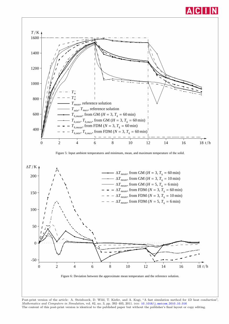
Figure 5: Input ambient temperatures and minimum, mean, andmaximum temperature of the solid.

0 2 4 6 8 10 12 14 16 18

-50

0

50

100

150

200

∆Tmean, from FDM (N = 5, Tk = 6 min)

∆Tmean, from FDM (N = 3, Tk = 10 min)

∆Tmean, from FDM (N = 3, Tk = 60 min)∆Tmean, from GM (H = 5, Tk = 6 min)

∆Tmean, from GM (H = 3, Tk = 10 min)

∆Tmean, from GM (H = 3, Tk = 60 min)

∆T /K

t /h

Figure 6: Deviation between the approximate mean temperature and the reference solution.



Together with the inputs and the reference solution, numerical results computed by means of both the proposedGM with the FOH-type integration method and the FDM with the Crank-Nicolson integration scheme are shown inFig. 5. It contains the minimum, the maximum, and the mean value of the temperature profile for each samplingperiod. To keep the figure uncluttered, only results for a fixed sampling timeTk = 60 min are shown. It is possible tofurther increase the sampling period, however, the achieved accuracy obviously deteriorates.

Two major sources of inaccuracies are the discretization ofthe spatial domain and the time domain. Refining theresolution of only one of these dimensions is less effective than refining the resolution of both dimensions at thesametime. For the GM this would mean to increaseH, the number of trial functions, which entails an increase interms ofthe computational load. Therefore, in this analysis,H never exceeds 5.

The deviations∆Tmean between the mean temperatures of the approximate results and the mean temperature ofthe reference solution are shown in Fig. 6 for variousH, N, andTk. The FDM with smallN underestimates thethermal inertia of the system, whereas with the GM this is only the case for large sampling periodsTk. Evidently, theimprovement fromH = 3 to H = 5 is only moderate.

The GM produces the largest deviations right after discontinuous changes of the inputs. However, the practicalrelevance of these transient errors is rather marginal. Moreover, the errors can be easily reduced if the samplingperiodsTk are decreased in the vicinity of discontinuous changes of the inputs.

In this analysis,λ(hi , Th(y, t)) is considered to be constant during the interval [tk, tk+1) and it depends only onxkand i ∈ {1, 2, . . . ,H}. Therefore, the accuracy could be further improved if bothxk and xk+1 were utilized in thecomputation ofλ for the interval [tk, tk+1). For simplicity, this idea was not followed in this work.

0 %

1 %

2 %

3 %

Normalized CPU time

H = N = 5Tk = 6 min

H = N = 3Tk = 10 min

H = N = 3Tk = 60 min

Solved with FDM

Solved with GM 3.0 %

1.4 %1.4 %

0.6 %0.9 %

0.1 %

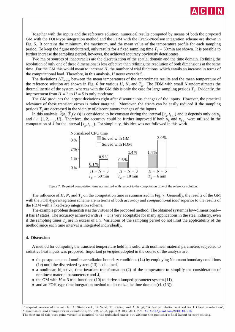
Figure 7: Required computation time normalized with respect to the computation time of the reference solution.

The influence ofH, N, andTk on the computation time is summarized in Fig. 7. Generally, the results of the GMwith the FOH-type integration scheme are in terms of bothaccuracyandcomputational loadsuperior to the results ofthe FDM with a fixed-step integration scheme.

The example problem demonstrates the virtues of the proposed method. The obtained system is low-dimensional—it hasH states. The accuracy achieved withH = 3 is very acceptable for many applications in the steel industry, evenif the sampling timesTk are in excess of 1 h. Variations of the sampling period do not limit the applicability of themethod since each time interval is integrated individually.

4. Discussion

A method for computing the transient temperature field in a solid with nonlinear material parameters subjected toradiative heat inputs was proposed. Importantprinciplesadopted in the course of the analysis are:

• the postponement of nonlinear radiation boundary conditions (14) by employing Neumann boundary conditions(1c) until the discretized system (13) is obtained,• a nonlinear, bijective, time-invariant transformation (2) of the temperature to simplify the consideration of

nonlinear material parametersc andλ,• the GM withH = 3 trial functions (10) to derive a lumped-parameter system (11),• and an FOH-type time integration method to discretize the time domain (cf. (13)).



Finally, the implicit algebraic equation (16) is obtained,which can be solved without difficulty. The most salientmodeling assumptionsmaterialized in this work can be summarized as follows:

• The geometries of the solid and the ambient surfaces are considered infinitely large along two spatial dimen-sions. The temperature field is assumed to be constant along these directions. The approximation seems justifiedif the length and the width of the solid significantly exceed its thicknessL or if many solids are densely arrangedside by side.• For the formulation of radiation boundary conditions, it isassumed that the surfaces are separated by a non-

participating gaseous medium.• The surfaces themselves are considered as diffuse gray bodies with homogeneous temperatures and constant

emissivitiesε∓w andε∓.

However, modeling assumptions are not the only compromise made in this analysis—there are also some significantmathematical approximations:

• The MWR suggests to approximate the temperature fieldT(y, t) by Th(y, t) taken from some finite-dimensionalspace. In this paper, the GM was utilized, whereTh(y, t) and the trial functionsv(y) are confined to the samespaceVh. A reasonable choice for the trial functionshi (i ∈ {1, 2, . . . ,H}) is vital for minimizing the entailedapproximation error.• It is assumed thatλ(hi, Th) ∀ i ∈ {1, 2, . . . ,H} in (11b) takes the constant valueλ(hi, Th(y, tk)) during each time

interval [tk, tk+1).• The inputq(t) is constrained to a piecewise linear signal (12), which mayjump attk. Therefore, sampling points

tk should be set at least at discontinuities ofq(t).• The radiation boundary conditions (14) are only satisfied atthe sampling pointstk, since they have been in-

troduced after discretization of the time domain. For theircomputation, the surface temperatureT(∓L/2, tk) isreplaced by its Galerkin approximation.• The implicit difference equation (16) is only numerically solved.

Despite these limitations, the proposed method proved to beadequate for many purposes, especially the intendedapplication in the steel industry.

Compared to the FDM, the GM yields a mathematical structure that is beneficial for control tasks. Themeanof the transformed temperatureT and, forH = 2 or H = 3, thesymmetryof the current temperature profile arereflected by the single state variablesx1(t) andx2(t) or x1,k andx2,k for the continuous-time or discrete-time system,respectively. Neglecting the temperature dependence ofλ(hi , Th(y, tk)) in (11b), which, anyhow, is weak,x1(t) andx2(t) are independent states of (11a), sinceA exhibits a diagonal structure. Moreover, the structure ofB suggests theregular input transformation

q(t) =

[

q−(t)q+(t)

]

=12

[

1 −11 1

] [

q1(t)q2(t)

]

to obtain twodecoupledsystems, whereq1(t) controls onlyx1(t) andq2(t) only x2(t). If the (stable) statex3(t) isignored as an output, the two systems are of the single-inputsingle-output type. Compared to the FDM, this approachsignificantly simplifies the design of a temperature controller which uses the ambient temperatures as inputs, becausethe original multi-input multi-output system (11) simplifies to two independent single-input single-output systems.The same input transformation can be applied without effort to the discrete-time system (13).

Some more advantages of the proposed method are acceptable accuracy with only three Galerkin trial functions(10), even for large sampling periods, robustness against variations of the sampling time, reliable convergence behav-ior, small model dimensions, and low computational costs. The latter properties may be of particular interest if themodel should be used in real-time applications. Therefore,the proposed method can be suitable for implementationsin trajectory planning, optimization, or control tasks, where constraints on the computing time are often tight.

Acknowledgments

The authors from Vienna University of Technology thankfully acknowledge the sustained support provided by AGder Dillinger Huttenwerke.



References

[1] H. D. Baehr, K. Stephan, Heat and Mass Transfer, 2nd ed., Springer-Verlag, Berlin Heidelberg, 2006.[2] L. Balbis, J. Balderud, M. J. Grimble, Nonlinear predictive control of steel slab reheating furnace, Proceedings ofthe American Control

Conference, Seattle, Washington, USA (2008) 1679–1684.[3] V. Berinde, Iterative Approximation of Fixed Points, vol. 1912 of Lecture Notes in Mathematics, Springer, Berlin, 2007.[4] BISRA, Physical constants of some commercial steels at elevated temperatures, Tech. rep., British Iron & Steel Research Association, London

(1953).[5] J. Crank, P. Nicholson, A practical method for numericalevaluation of solutions of partial differential equations of the heat conduction type,

Proc. Cambridge Philos. Soc. 43 (1947) 50–67.[6] G. v. Ditzhuijzen, D. Staalman, A. Koorn, Identificationand model predictive control of a slab reheating furnace, Proceedings of the 2002

IEEE International Conference on Control Applications, Glasgow, UK (2002) 361–366.[7] L. C. Evans, Partial Differential Equations, vol. 19 of Graduate Studies in Mathematics, American Mathematical Society, Providence, Rhode

Island, 2002.[8] C. Fletcher, Computational Galerkin Methods, Springer, New York, 1984.[9] G. F. Franklin, J. D. Powell, M. Workman, Digital Controlof Dynamic Systems, 3rd ed., Prentice Hall, Upper Saddle River, 1997.

[10] K. Harste, Untersuchung zur Schrumpfung und zur Entstehung von mechanischen Spannungen wahrend der Erstarrung und nachfolgenderAbkuhlung zylindrischer Blocke aus Fe-C-Legierungen, Ph.D. thesis, Technische Universitat Clausthal (1989).

[11] H. C. Hottel, A. F. Sarofim, Radiative Transfer, McGraw-Hill, New York, 1967.[12] J. H. Lienhard IV, J. H. Lienhard V, A Heat Transfer Textbook, 3rd ed., Phlogiston Press, Cambridge, Massachusetts, 2002.[13] M. F. Modest, Radiative Heat Transfer, 2nd ed., Academic Press, New York, 2003.[14] K. Ogata, Discrete-Time Control Systems, 2nd ed., Prentice Hall, Upper Saddle River, 1995.[15] C. Philipps, H. Nagle, Digital Control System Analysisand Design, 3rd ed., Prentice Hall, Englewood Cliffs, 1995.[16] B. D. Reddy, Introductory Functional Analysis, Texts in Applied Mathematics, Springer, New York, 1997.[17] L. F. Shampine, M. W. Reichelt, J. A. Kierzenka, Solvingindex-1 DAEs in MATLAB and Simulink, SIAM Review 41 (1999) 538–552.[18] H. Sibarani, Y. Samyudia, Robust nonlinear slab temperature control design for an industrial reheating furnace, Computer Aided Chemical

Engineering 18 (2004) 811–816.[19] R. D. Skeel, M. Berzins, A method for the spatial discretization of parabolic equations in one space variable, SIAM Journal on Scientific and

Statistical Computing 11 (1990) 1–32.[20] A. Steinboeck, D. Wild, T. Kiefer, A. Kugi, A flexible time integration method for the 1D heat conduction problem, Proceedings of the 6th

Vienna Conference on Mathematical Modelling, Vienna, Austria, ARGESIM Report no. 35 (2009) 1204–1214.[21] D. Wild, T. Meurer, A. Kugi, Modelling and experimentalmodel validation for a pusher-type reheating furnace, Mathematical and Computer

Modelling of Dynamical Systems 15 (3) (2009) 209–232.[22] N. Yoshitani, T. Ueyama, M. Usui, Optimal slab heating control with temperature trajectory optimization, Proceedings of the 20th International

Conference on Industrial Electronics, Control and Instrumentation, IECON’94 3 (1994) 1567–1572.[23] B. Zhang, Z. Chen, L. Xu, J. Wang, J. Zhang, H. Shao, The modeling and control of a reheating furnace, Proceedings of the American Control

Conference, Anchorage, Alaska, USA (2002) 3823–3828.[24] O. C. Zienkiewicz, K. Morgan, Finite Elements and Approximation, Wiley, New York, 1983.



a fast simulation method for 1d heat conduction · a fast simulation method for 1d heat conduction...

Documents