A Few Useful Things to Know about Machine Learning

Pedro DomingosDepartment of Computer Science and Engineering University of Washington"

2012"

A Few Useful Things to Know about Machine Learning

• Machine learning systems automatically learn programs from data,

• Machine learning is used in Web search, spam filters, recommender systems, ad placement, credit scoring, fraud detection, stock trading, drug design, and many other applications.

• Several fine textbooks are available to interested practitioners and researchers. However, much of the “folk knowledge” that is needed to successfully develop machine learning applications is not readily available in them.

• So, many machine learning projects take much longer than necessary or produce less- than-ideal results

A Few Useful Things to Know about Machine Learning

• The focus is on the most mature and widely used machine learnings: classification.

• A classifier is a system that inputs (typically) a vector of discrete and/or continuous feature values and outputs a single discrete value, the class.

• A learner inputs a training set of examples, and outputs a classifier. The test of the learner is whether this classifier produces the correct output for future examples

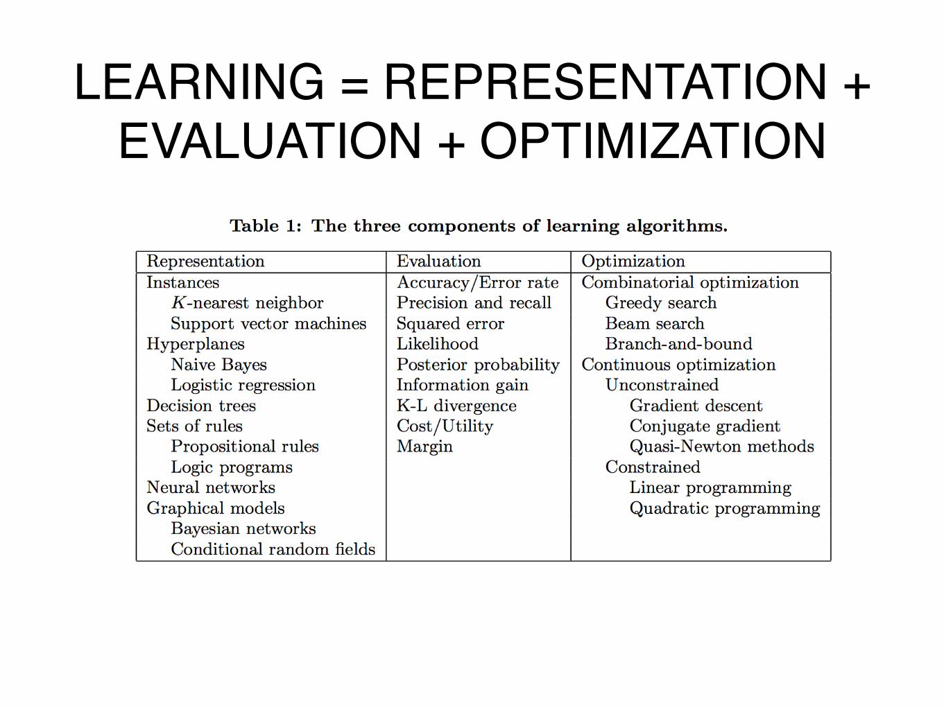
LEARNING = REPRESENTATION +"EVALUATION + OPTIMIZATION"

• Learning algorithms consists of combinations of just three components:

✦ Representation: choosing the set of classifiers that it can possibly learn. This set is called the hypothesis space of the learner. If a classifier is not in the hypothesis space, it cannot be learned

✦ Evaluation: An evaluation function (also called objective function or scoring function) is needed to distinguish good classifiers from bad ones. The evaluation function used internally by the algorithm may differ from the external one that we want the classifier to optimize "

✦ Optimization:needing a method to search among the classifiers in the language for the highest-scoring one. The choice of optimization technique is key to the efficiency of the learner

LEARNING = REPRESENTATION +"EVALUATION + OPTIMIZATION

LEARNING = REPRESENTATION +"EVALUATION + OPTIMIZATION

• Not all combinations of one component from each column of Table make equal sense. For example, discrete representations naturally go with combinatorial optimization, and continuous ones with continuous optimization.

• Most textbooks are organized by representation, the other components are equally important

"

IT’S GENERALIZATION THAT COUNTS

• The fundamental goal of machine learning is to generalize beyond the examples in the training set.

• The most common mistake among machine learning beginners is to test on the training data and have the illusion of success.

• cross-validation: randomly dividing your training data into (say) ten subsets, holding out each one while training on the rest, testing each learned classifier on the examples it did not see, and averaging the results "

DATA ALONE IS NOT ENOUGH

• Every learner must embody some knowledge or assumptions beyond the data it’s given.

• Very general assumptions—like smoothness, similar examples having similar classes, limited dependences, or limited complexity—are often enough to do very well, and this is a large part of why machine learning has been so successful.

• one of the key criteria for choosing a representation is which kinds of knowledge are easily expressed in it:

✦ if we have a lot of knowledge about what makes examples similar in our domain, instance- based methods may be a good choice.

✦ If we have knowledge about probabilistic dependencies, graphical models are a good fit.

✦ And if we have knowledge about what kinds of preconditions are required by each class, “IF . . . THEN . . .” rules may be the the best option. ""

OVERFITTING HAS MANY FACES

• What if the knowledge and data we have are not sufficient to completely determine the correct classifier? Then we run the risk of just hallucinating a classifier (or parts of it) that is not grounded in reality.

• When your learner outputs a classifier that is 100% accurate on the training data but only 50% accurate on test data, when in fact it could have output one that is 75% accurate on both, it has overfit "

• This problem is called overfitting, and is the bugbear of machine learning, "

""

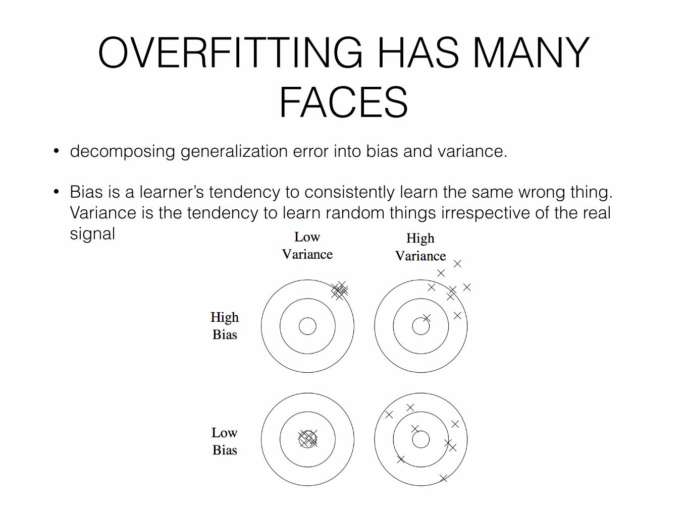
• decomposing generalization error into bias and variance.

• Bias is a learner’s tendency to consistently learn the same wrong thing. Variance is the tendency to learn random things irrespective of the real signal

"

"

"

"

""

OVERFITTING HAS MANY FACES

OVERFITTING HAS MANY FACES

• A linear learner has high bias, because when the frontier between two classes is not a hyperplane the learner is unable to induce it,

• Decision trees don’t have this problem because they can represent any Boolean function, but on the other hand they can suffer from high variance: decision trees learned on different training sets generated by the same phenomenon are often very different, when in fact they should be the same.

• Similar reasoning applies to the choice of optimization method: beam search has lower bias than greedy search, but higher variance, because it tries more hypotheses.

• Thus, contrary to intuition, a more powerful learner is not necessarily better than a less powerful one

OVERFITTING HAS MANY FACES

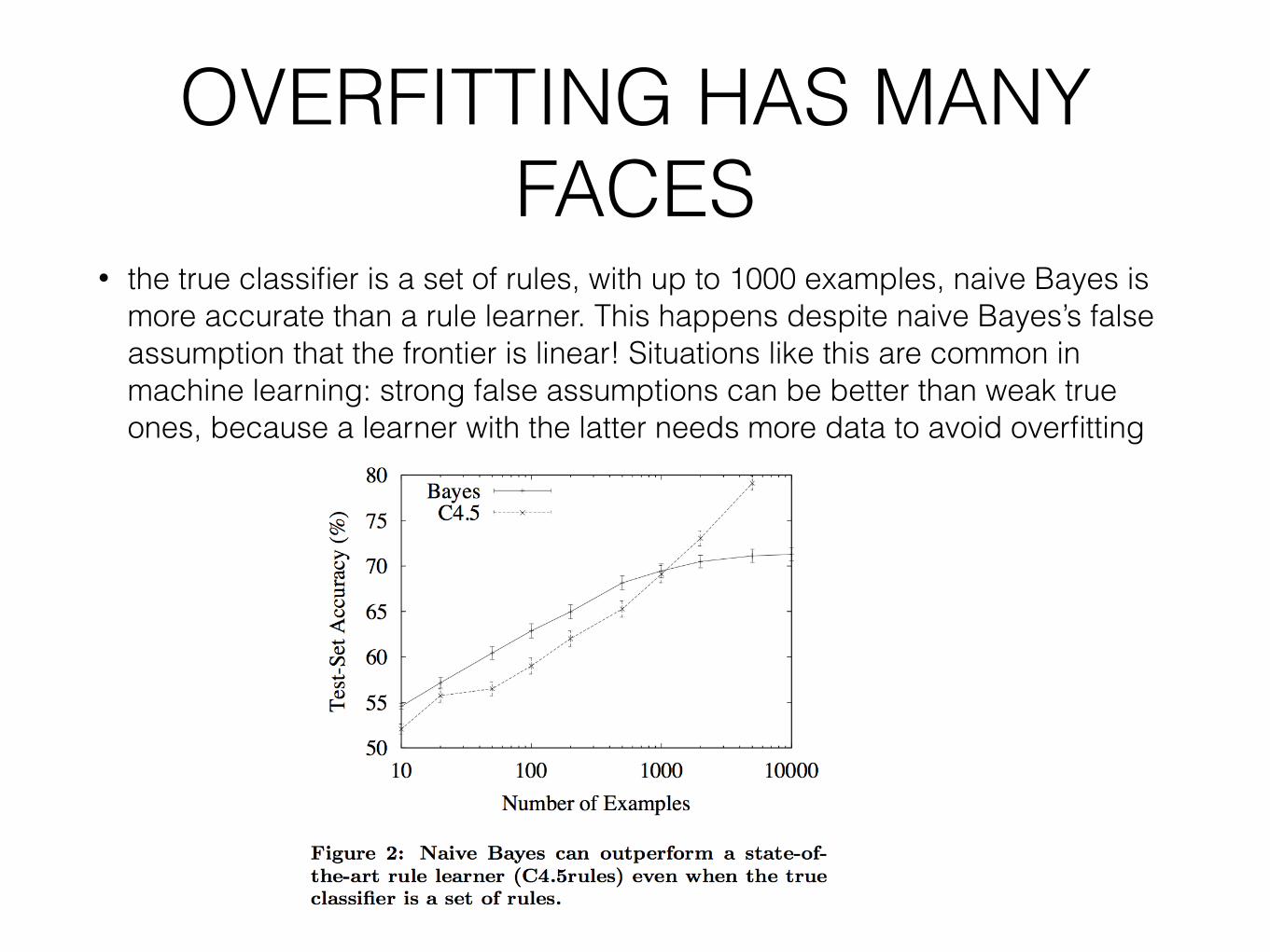
• the true classifier is a set of rules, with up to 1000 examples, naive Bayes is more accurate than a rule learner. This happens despite naive Bayes’s false assumption that the frontier is linear! Situations like this are common in machine learning: strong false assumptions can be better than weak true ones, because a learner with the latter needs more data to avoid overfitting """"""""""""""""""

OVERFITTING HAS MANY FACES

• methods to combat overfitting:

• cross-validation

• adding a regularization term to the evaluation function. This can, for example, penalize classifiers with more structure, thereby favoring smaller ones with less room to overfit.

• statistical significance test like chi-square: before adding new structure, to decide whether the distribution of the class really is different with and without this structure (particularly useful when data is very scarce)

• A common misconception about overfitting is that it is caused by noise, like training examples labeled with the wrong class.

• But severe overfitting can occur even in the absence of noise. For instance, suppose we learn a Boolean classifier that is just the disjunction of the examples labeled “true” in the training set, This classifier gets all the training examples right and every positive test example wrong, regardless of whether the training data is noisy or not

INTUITION FAILS IN HIGH"DIMENSIONS"

• curse of dimensionality: many algorithms that work fine in low dimensions become intractable when the input is high-dimensional.

• similarity-based reasoning that machine learning algorithms depend on, breaks down in high dimensions: (nearest neighbor classifier with Hamming distance)

• there is an effect that partly counteracts the curse, which might be called the“blessing of non-uniformity.” In some applications examples are not spread uniformly throughout the instance space, but are concentrated on or near a lower-dimensional manifold

• k-nearest neighbor works quite well for handwritten digit recognition even though images of digits have one dimension per pixel, because the space of digit images is much smaller than the space of all possible images.

FEATURE ENGINEERING IS THE KEY

• some machine learning projects succeed and some fail. What makes the difference? the most important factor is the features used.

• Often,the raw data is not in a form that is amenable to learning, but you can construct features from it.

• machine learning is not a one-shot process of building a data set and running a learner, but rather an iterative process of running the learner, analyzing the results, modifying the data and/or the learner, and repeating

MORE DATA BEATS A CLEVERER"ALGORITHM

• Suppose you’ve constructed the best set of features you can, but the classifiers you’re getting are still not accurate enough. What can you do now? There are two main choices:

✦ design a better learning algorithm or,

✦ gather more data (more examples, and possibly more raw features, subject to the curse of dimensionality)

• As a rule of thumb, a dumb algorithm with lots and lots of data beats a clever one with modest amounts of it.

• two main limited resources are time and memory. Enormous mountains of data are available, but there is not enough time to process it, so it goes unused.

• This leads to a paradox: even though in principle more data means that more complex classifiers can be learned, in practice simpler classifiers used, because complex ones take too long to learn.

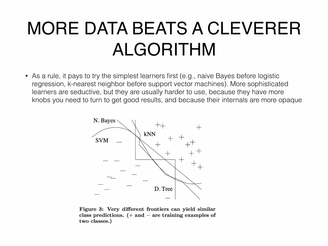
MORE DATA BEATS A CLEVERER"ALGORITHM

• As a rule, it pays to try the simplest learners first (e.g., naive Bayes before logistic regression, k-nearest neighbor before support vector machines). More sophisticated learners are seductive, but they are usually harder to use, because they have more knobs you need to turn to get good results, and because their internals are more opaque

"

"

"

"

"

"

"

LEARN MANY MODELS, NOT JUST ONE

• Before, everyone had their favorite learner, with some reasons to believe in its superiority. Most effort went into trying many variations of it and selecting the best one.

• the best learner varies from application to application, and systems containing many different learners started to appear.

• if instead of selecting the best variation found, we combine many variations, the results are better "

"

LEARN MANY MODELS, NOT JUST ONE

• In bagging, we simply generate random variations of the training set by resampling, learn a classifier on each, and combine the results by voting. This works because it greatly reduces variance while only slightly increasing bias.

• In boosting, training examples have weights, and these are varied so that each new classifier focuses on the examples the previous ones tended to get wrong.

• In stacking, the outputs of individual classifiers become the inputs of a “higher-level” learner that figures out how best to combine them.

• the random forest algorithm combines random decision trees with bagging to achieve very high classification accuracy

Top 10 algorithms in data mining

• Xindong Wu · Vipin Kumar · J. Ross Quinlan · Joydeep Ghosh · Qiang Yang · Hiroshi Motoda · Geoffrey J. McLachlan · Angus Ng · Bing Liu · Philip S. Yu · Zhi-Hua Zhou · Michael Steinbach · David J. Hand · Dan Steinberg

Top 10 algorithms in data mining

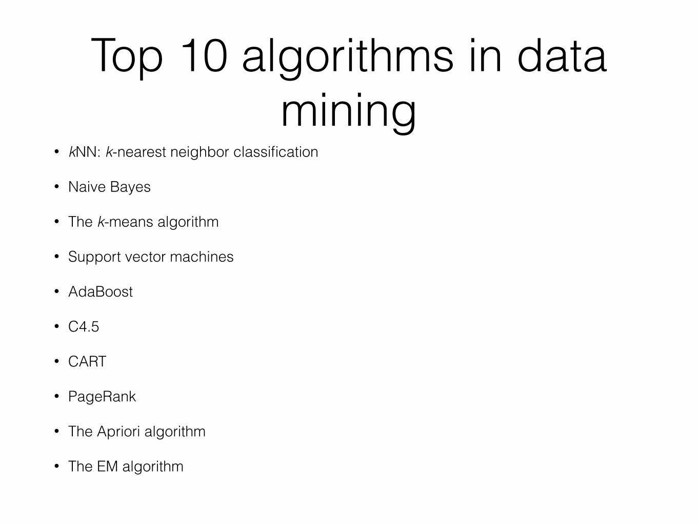
• kNN: k-nearest neighbor classification

• Naive Bayes

• The k-means algorithm

• Support vector machines

• AdaBoost

• C4.5

• CART

• PageRank

• The Apriori algorithm

• The EM algorithm

AdaBoost

• Ensemble learning deals with methods which employ multiple learners to solve a problem.

• The AdaBoost algorithm is one of the most important ensemble methods, since it has solid theoretical foundation, very accurate prediction, great simplicity, and wide and successful applications

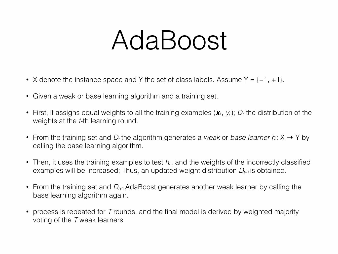
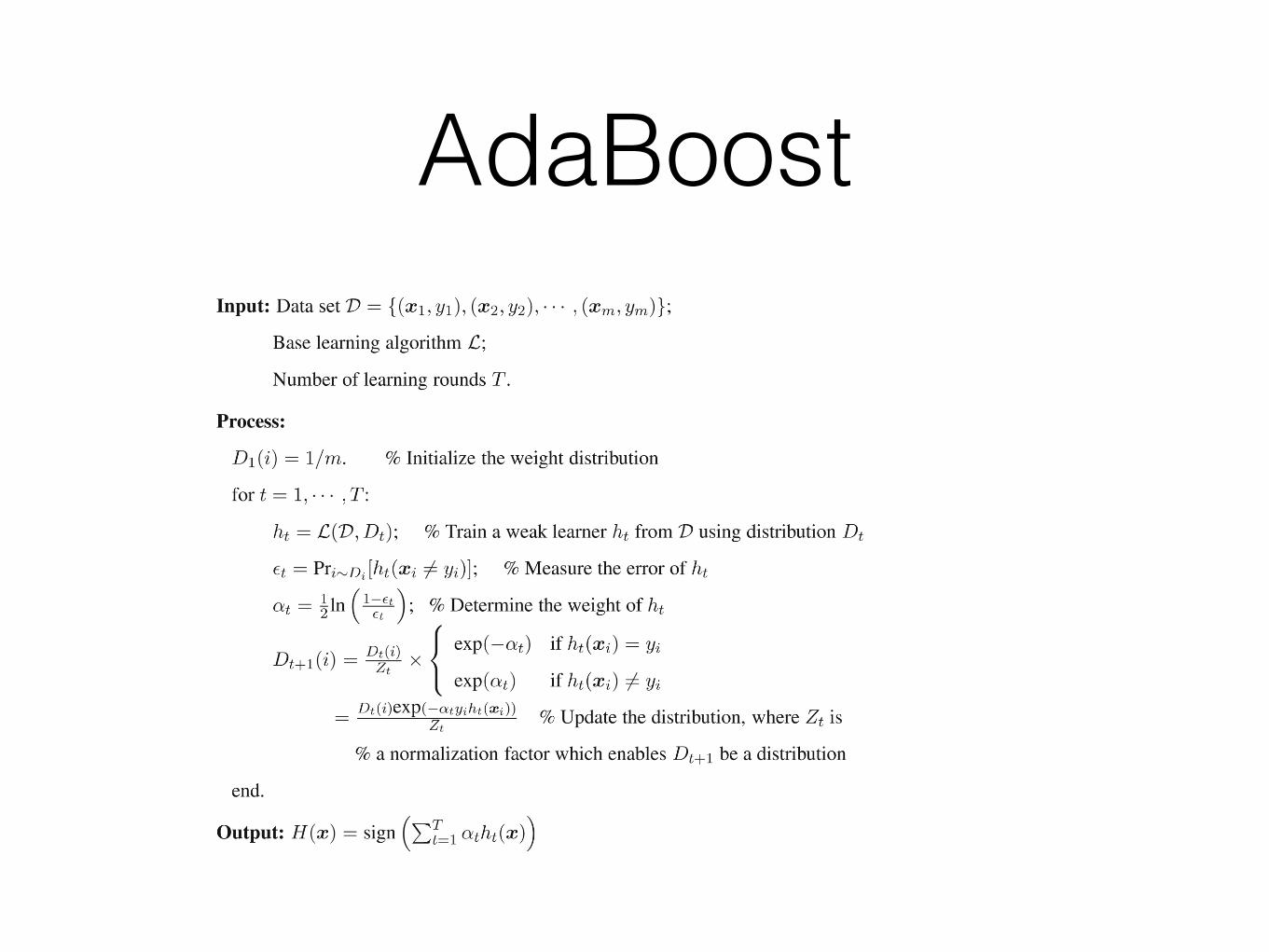
• X denote the instance space and Y the set of class labels. Assume Y = {−1, +1}.

• Given a weak or base learning algorithm and a training set.

• First, it assigns equal weights to all the training examples (xi , yi ); Dt the distribution of the weights at the t-th learning round.

• From the training set and Dt the algorithm generates a weak or base learner ht : X → Y by calling the base learning algorithm.

• Then, it uses the training examples to test ht , and the weights of the incorrectly classified examples will be increased; Thus, an updated weight distribution Dt+1 is obtained.

• From the training set and Dt+1 AdaBoost generates another weak learner by calling the base learning algorithm again.

• process is repeated for T rounds, and the final model is derived by weighted majority voting of the T weak learners

AdaBoost

AdaBoost

• We are given a set of records and columns.Each column corresponds to an attribute. One of these attributes represents the category of the record.

• The problem is to determine a decision tree that on the basis of answers to questions about the non-category attributes predicts correctly the value of the category attribute.

C4.5

• The basic ideas are that:

✦ In the decision tree each node corresponds to an attribute and each arc corresponds to a possible value of that attribute.

✦ In the decision tree each node should be associated with the attribute which is most informative among the attributes not yet considered in the path from the root.

✦ Entropy is used to measure how informative is a node.

C4.5

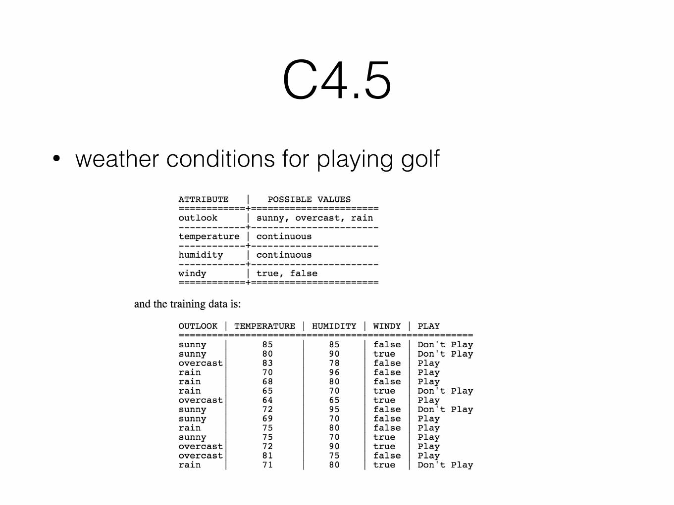
• weather conditions for playing golf

"

"

"

"

C4.5

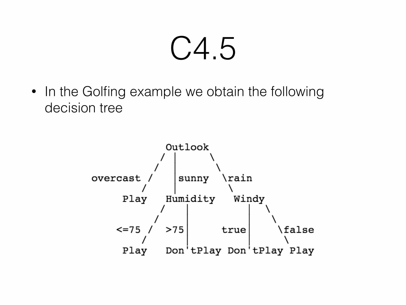
• In the Golfing example we obtain the following decision tree

"

"

"

"

C4.5

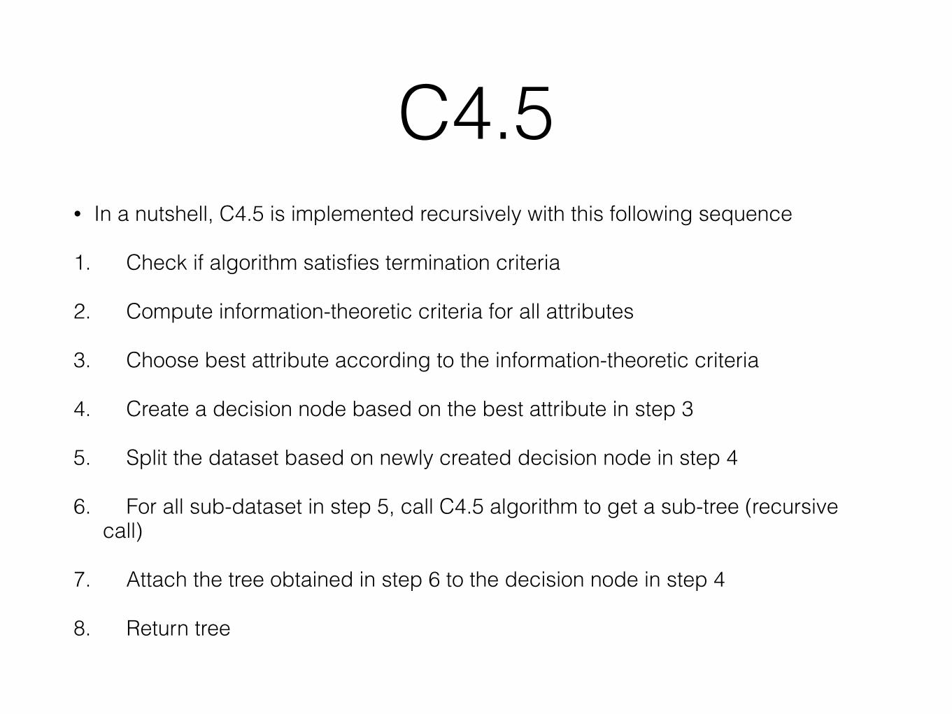
• In a nutshell, C4.5 is implemented recursively with this following sequence

1. Check if algorithm satisfies termination criteria

2. Compute information-theoretic criteria for all attributes

3. Choose best attribute according to the information-theoretic criteria

4. Create a decision node based on the best attribute in step 3

5. Split the dataset based on newly created decision node in step 4

6. For all sub-dataset in step 5, call C4.5 algorithm to get a sub-tree (recursive call)

7. Attach the tree obtained in step 6 to the decision node in step 4

8. Return tree

C4.5

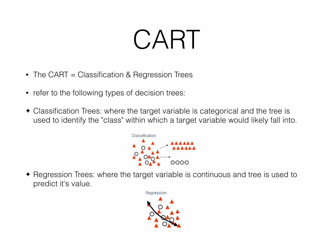
CART• The CART = Classification & Regression Trees

• refer to the following types of decision trees:

✦ Classification Trees: where the target variable is categorical and the tree is used to identify the "class" within which a target variable would likely fall into.

"

"

✦ Regression Trees: where the target variable is continuous and tree is used to predict it's value.

"

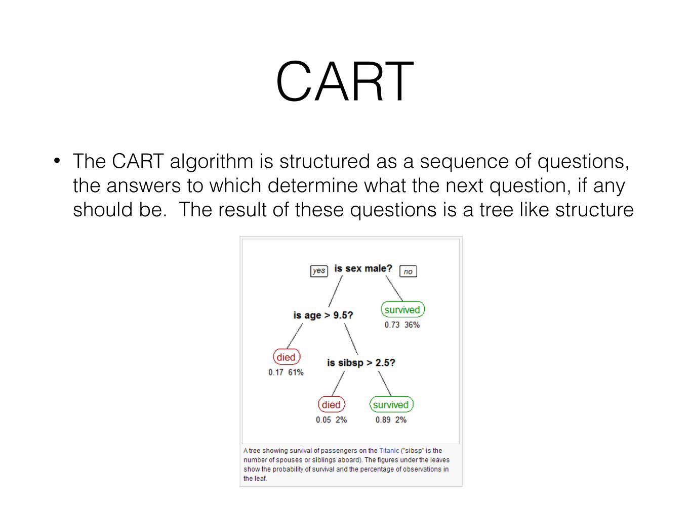
• The CART algorithm is structured as a sequence of questions, the answers to which determine what the next question, if any should be. The result of these questions is a tree like structure

"

"

"

"

CART

• Characteristics of the CART algorithm:

1. Each splitting is binary and considers one feature at a time.

2. Splitting criterion is the information gain or the Gini index

CART

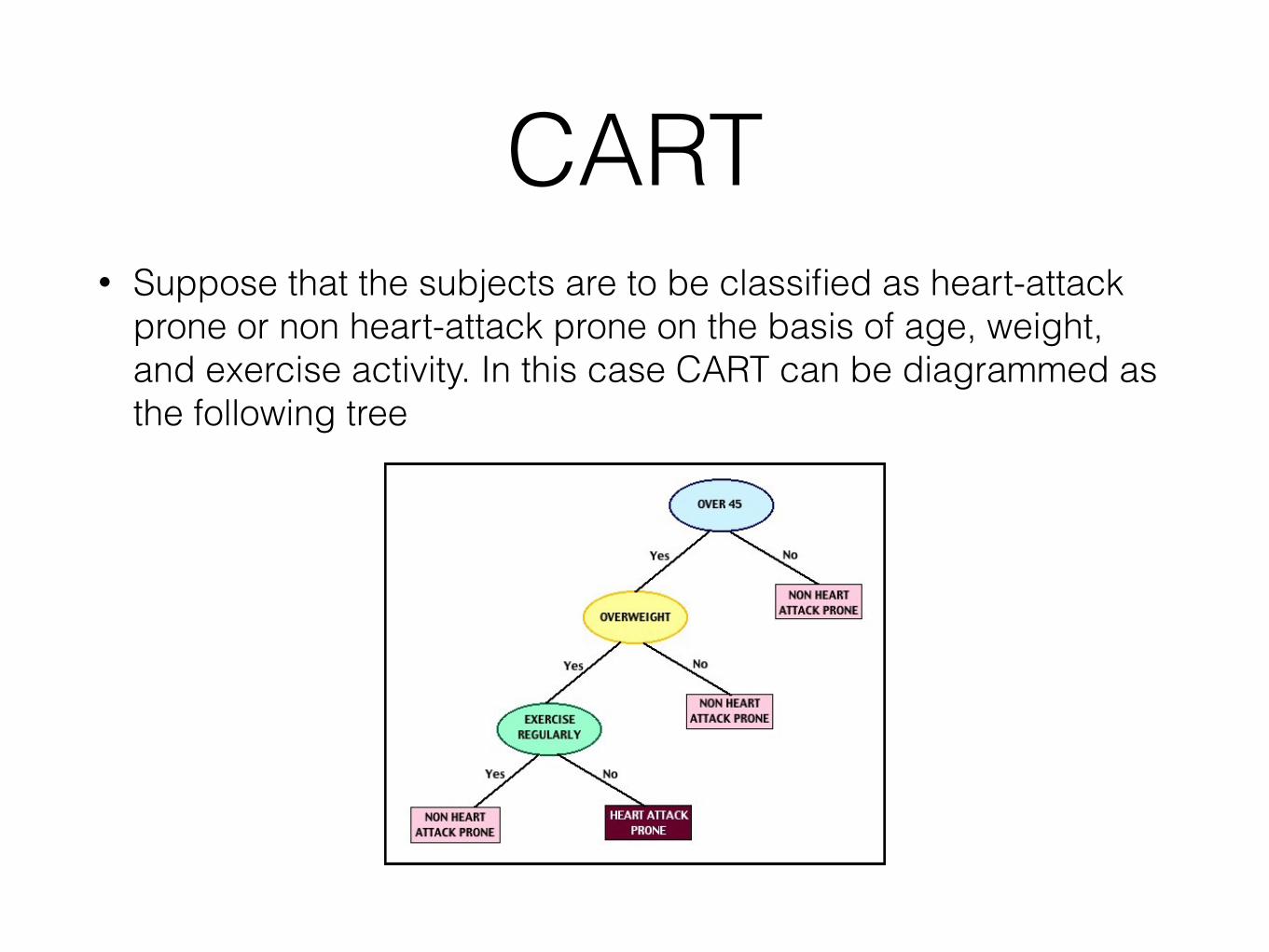
• Suppose that the subjects are to be classified as heart-attack prone or non heart-attack prone on the basis of age, weight, and exercise activity. In this case CART can be diagrammed as the following tree

"

"

"

"

CART

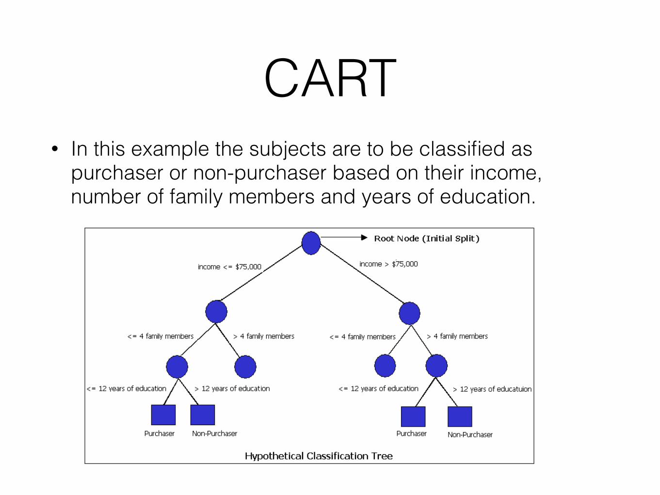
• In this example the subjects are to be classified as purchaser or non-purchaser based on their income, number of family members and years of education.

"

"

"

"

CART

• Some useful features and advantages of CART:

✦ CART is nonparametric and therefore does not rely on data belonging to a particular type of distribution.

✦ CART is not significantly impacted by outliers in the input variables.

✦ CART can use the same variables more than once in different parts of the tree. This capability can uncover complex interdependencies between sets of variables.

✦ CART can be used in conjunction with other prediction methods to select the input set of variables.

CART

PageRank • It is a search ranking algorithm using hyperlinks on the Web

• Based on the algorithm, they built the search engine Google, which has been a huge success.

• PageRank interprets a hyperlink from page x to page y as a vote, by page x, for page y.

• The underlying assumption is that more important websites are likely to receive more links from other websites

• It also analyzes the page that casts the vote. Votes casted by pages that are themselves “important” weigh more heavily and help to make other pages more “important”. This is exactly the idea of rank prestige in social networks

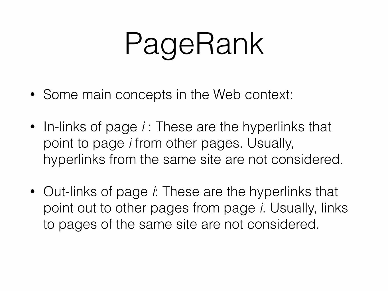
• Some main concepts in the Web context:

• In-links of page i : These are the hyperlinks that point to page i from other pages. Usually, hyperlinks from the same site are not considered.

• Out-links of page i: These are the hyperlinks that point out to other pages from page i. Usually, links to pages of the same site are not considered.

""

PageRank

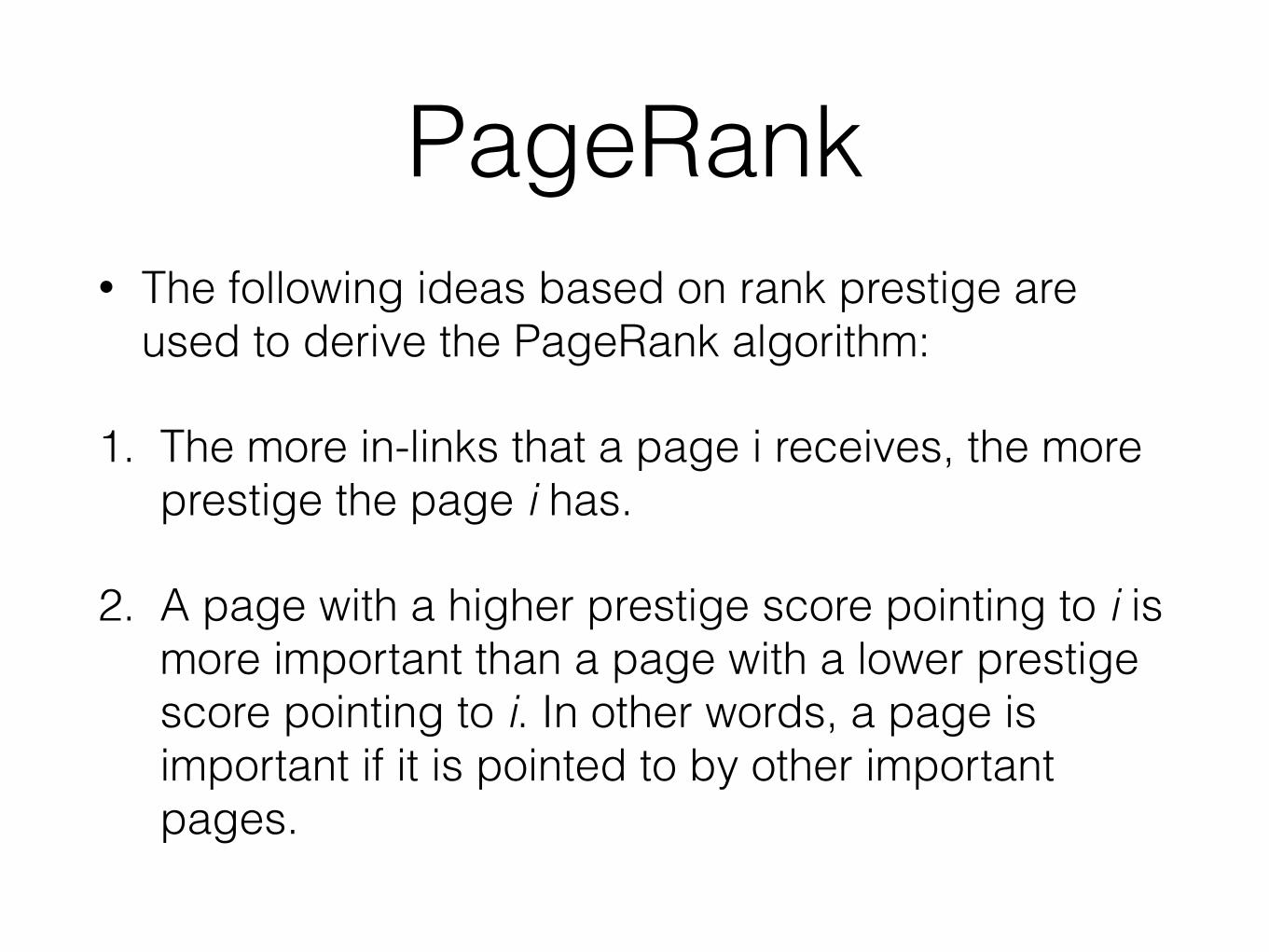
• The following ideas based on rank prestige are used to derive the PageRank algorithm:

1. The more in-links that a page i receives, the more prestige the page i has.

2. A page with a higher prestige score pointing to i is more important than a page with a lower prestige score pointing to i. In other words, a page is important if it is pointed to by other important pages.

PageRank

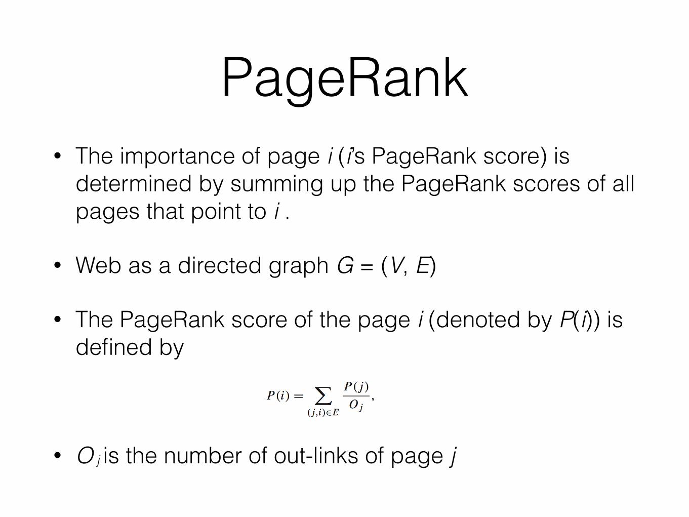
• The importance of page i (i’s PageRank score) is determined by summing up the PageRank scores of all pages that point to i .

• Web as a directed graph G = (V, E)

• The PageRank score of the page i (denoted by P(i)) is defined by

"

• O j is the number of out-links of page j

PageRank

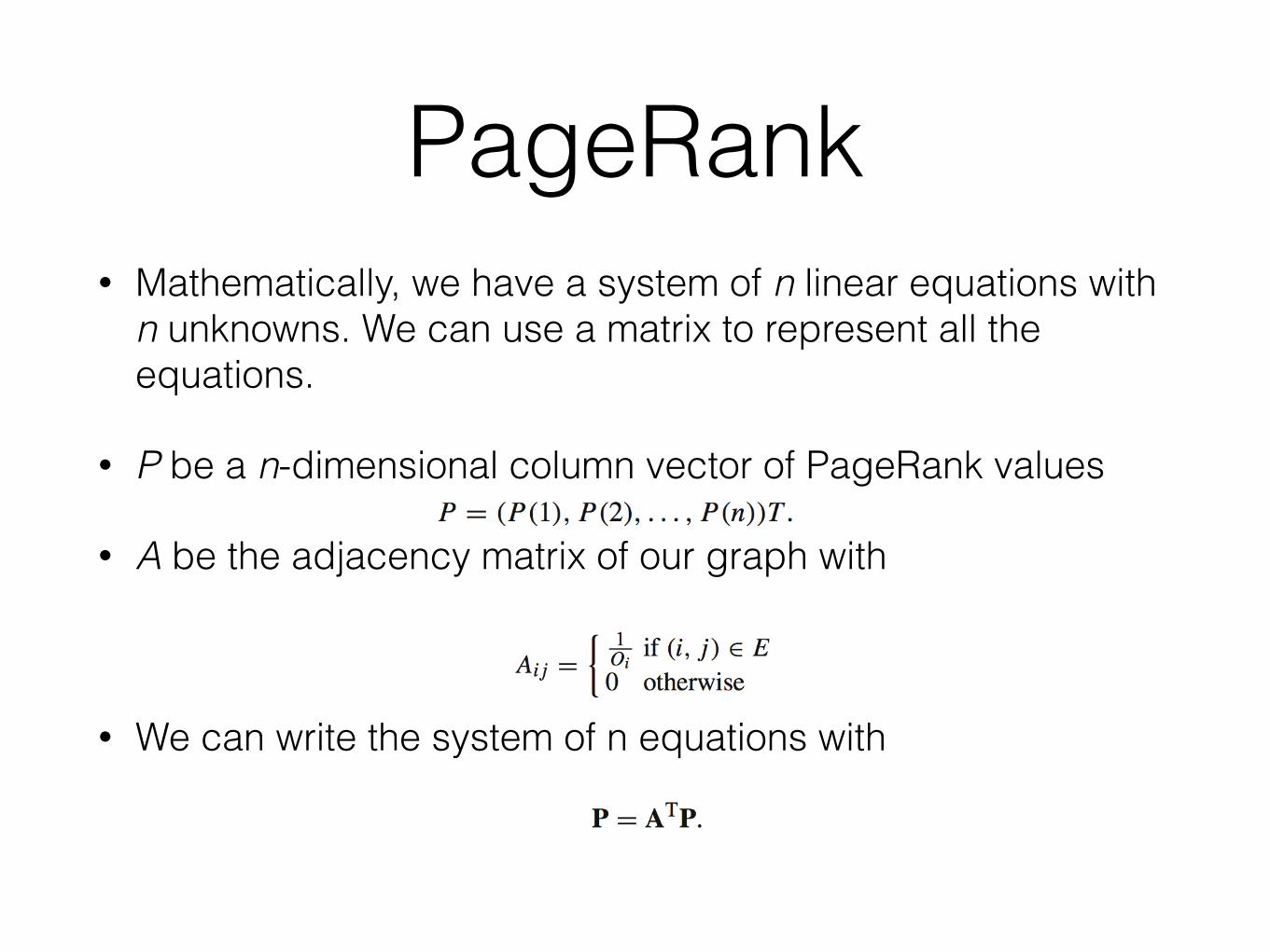
• Mathematically, we have a system of n linear equations with n unknowns. We can use a matrix to represent all the equations.

• P be a n-dimensional column vector of PageRank values

• A be the adjacency matrix of our graph with

"

• We can write the system of n equations with """

PageRank

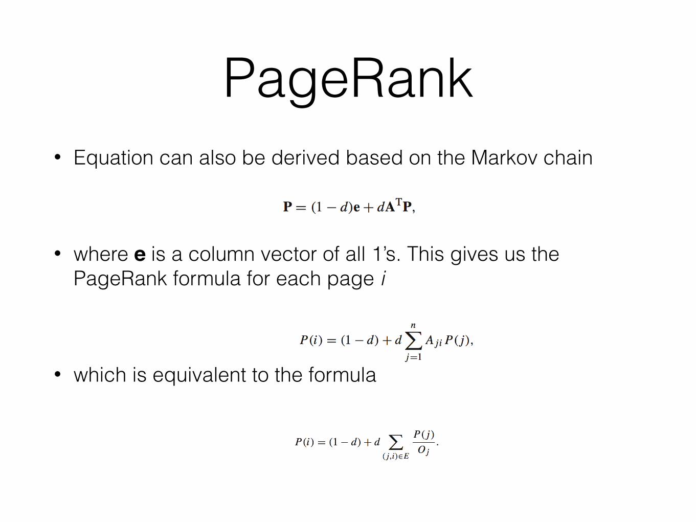
• Equation can also be derived based on the Markov chain

"

• where e is a column vector of all 1’s. This gives us the PageRank formula for each page i

"

• which is equivalent to the formula

"""

PageRank

• The computation of PageRank values of the Web pages can be done using the power iteration method

• The iteration ends when the PageRank values do not change much or converge.

• Since in Web search, we are only interested in the ranking of the pages, the actual convergence may not be necessary. Thus, fewer iterations are needed.

• it is reported that on a database of 322 million links the algorithm converges to an acceptable tolerance in roughly 52 iterations.

PageRank